
Change Orders In Illinois - McGovern & Greene · Change Orders In Illinois Lost Productivity And...
79
Change Orders In Illinois Lost Productivity And Efficiency Measurement Approaches Presentation by Jack A. Lazarczyk, CPA, CCC McGovern & Greene LLP
Transcript of Change Orders In Illinois - McGovern & Greene · Change Orders In Illinois Lost Productivity And...
Change Orders In Illinois Lost Productivity And Efficiency
Measurement Approaches
Presentation by
Jack A. Lazarczyk, CPA, CCC
McGovern & Greene LLP

Cumulative Impact - Definition “The costs associated with impact on distant work, which are not
as readily foreseeable or, if foreseeable, not as readily
computable as direct impact costs. The source of such costs is
the sheer number of and scope of changes to the contract. The
result is an unanticipated loss of efficiency and productivity
which increases the contractor’s performance costs and
usually extends his stay on the job.”
What is Productivity
Productivity is a measurement of rate of
output per unit of time or effort.
For example:
Productivity = Output / Input
Or
Productivity = Units / work-hours
Lost Productivity
Lost Productivity occurs when a contractor does not accomplish its anticipated rate of production. I.E. The contractor produces less than planned output per work hour of input.
Stated another way, the contractor expends more effort per unit of production than originally planned.
Production v Productivity
• Terms are not interchangeable
• Production is the measure of output.
• Productivity is the measure of production.
• A contractor can achieve its planned production without achieving its planned productivity.
• For example, a contractor could meet its planned production of pouring 1,000 cf of concrete per day, but expend twice the amount of planned labor to do so.
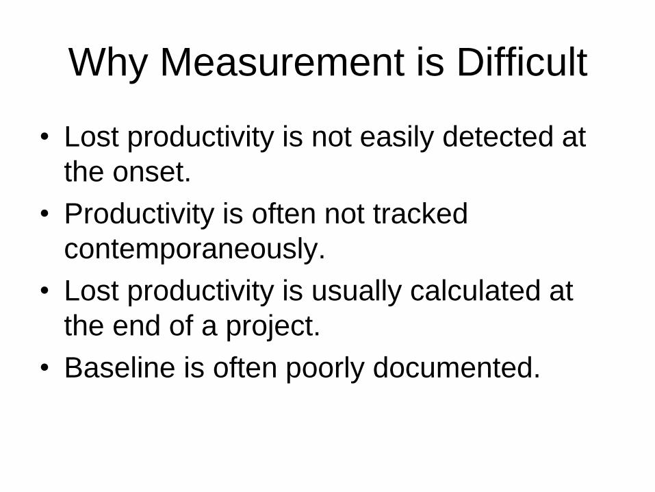
Why Measurement is Difficult
• Lost productivity is not easily detected at
the onset.
• Productivity is often not tracked
contemporaneously.
• Lost productivity is usually calculated at
the end of a project.
• Baseline is often poorly documented.
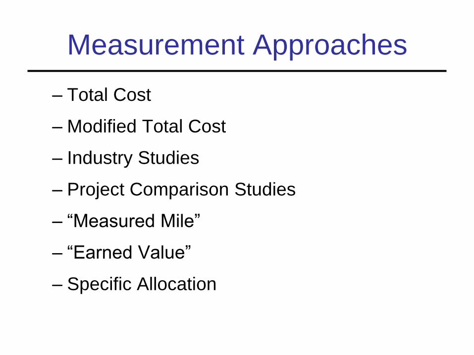
Measurement Approaches
– Total Cost
– Modified Total Cost
– Industry Studies
– Project Comparison Studies
– “Measured Mile”
– “Earned Value”
– Specific Allocation
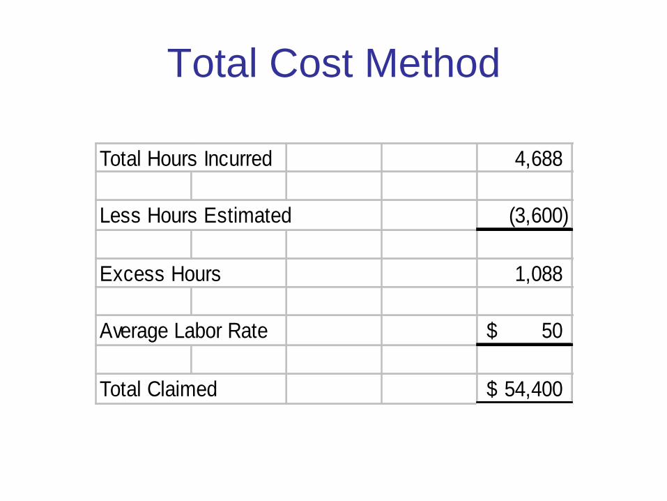
Total Cost Method
Total Hours Incurred 4,688
Less Hours Estimated (3,600)
Excess Hours 1,088
Average Labor Rate 50$
Total Claimed 54,400$

Modified Total Cost
Total Hour Incurred 4,688
Less Hours Estimated (3,600)
Excess Hours 1,088
Less: Change Orders (100)
Hours Under Bid (150)
Less XYZ's Errors (75)
Net Excess Hours 763
Average Labor Rate 50$
Total Claimed 38,150$
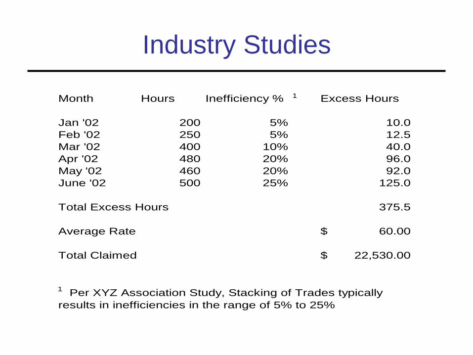
Industry Studies
Month Hours Inefficiency % 1 Excess Hours
Jan '02 200 5% 10.0
Feb '02 250 5% 12.5
Mar '02 400 10% 40.0
Apr '02 480 20% 96.0
May '02 460 20% 92.0
June '02 500 25% 125.0
Total Excess Hours 375.5
Average Rate 60.00$
Total Claimed 22,530.00$
1 Per XYZ Association Study, Stacking of Trades typically
results in inefficiencies in the range of 5% to 25%
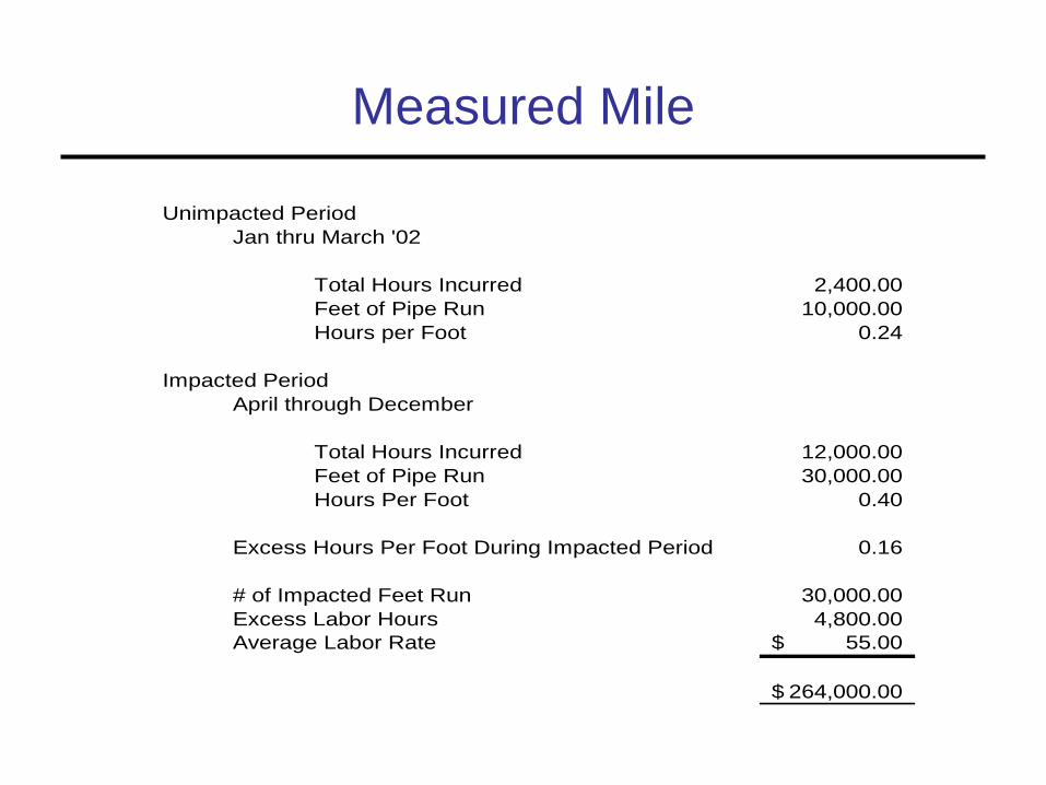
Measured Mile
Unimpacted Period
Jan thru March '02
Total Hours Incurred 2,400.00
Feet of Pipe Run 10,000.00
Hours per Foot 0.24
Impacted Period
April through December
Total Hours Incurred 12,000.00
Feet of Pipe Run 30,000.00
Hours Per Foot 0.40
Excess Hours Per Foot During Impacted Period 0.16
# of Impacted Feet Run 30,000.00
Excess Labor Hours 4,800.00
Average Labor Rate 55.00$
264,000.00$
Earned Value Method
• Earned Value analysis is a method for
measuring project performance. It indicates
how much of the budget should have been
spent in view of the amount of work done
so far and the baseline costs for the tasks,
assignments, or resources.
Most Common Measurements:
• Schedule Variance is a subjective indicator that does not reveal the critical path. A positive schedule variance is an indication that work in process is ahead of schedule.
• Cost Variance is an objective indicator stating the value of what was accomplished for the resources expended. A positive cost variance indicates that work was accomplished with less resources than planned
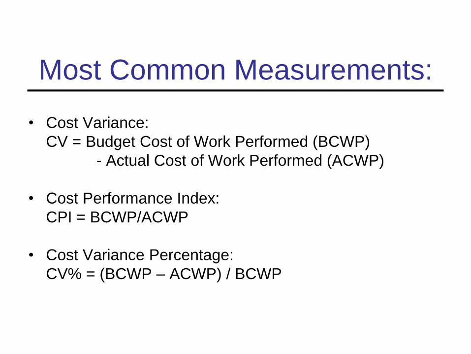
Most Common Measurements:
• Cost Variance:
CV = Budget Cost of Work Performed (BCWP)
- Actual Cost of Work Performed (ACWP)
• Cost Performance Index:
CPI = BCWP/ACWP
• Cost Variance Percentage:
CV% = (BCWP – ACWP) / BCWP
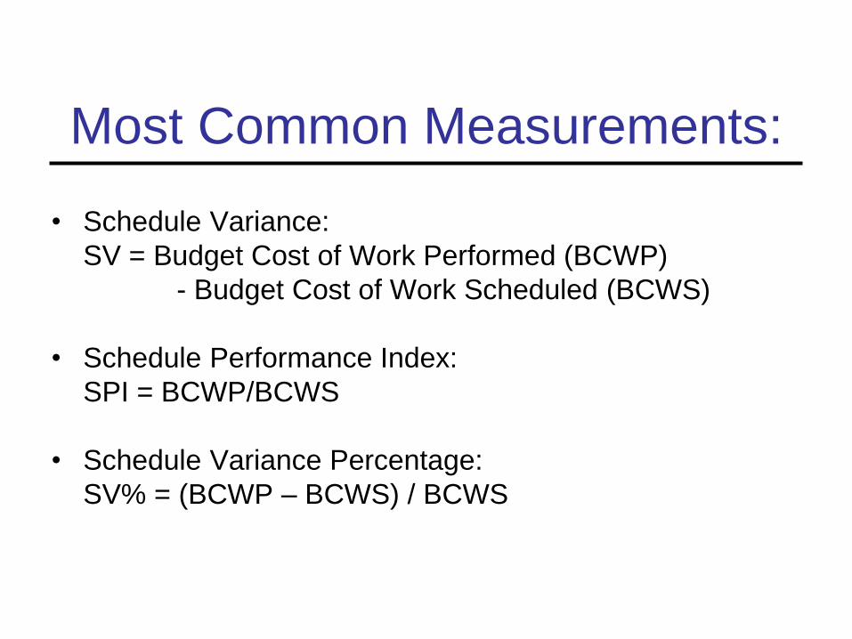
Most Common Measurements:
• Schedule Variance:
SV = Budget Cost of Work Performed (BCWP)
- Budget Cost of Work Scheduled (BCWS)
• Schedule Performance Index:
SPI = BCWP/BCWS
• Schedule Variance Percentage:
SV% = (BCWP – BCWS) / BCWS
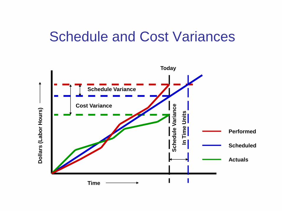
Schedule and Cost Variances
Time
Do
lla
rs (
La
bo
r H
ou
rs)
Schedule Variance
Cost Variance
Sc
he
du
le V
ari
an
ce
In T
ime
Un
its
Today
Performed
Scheduled
Actuals
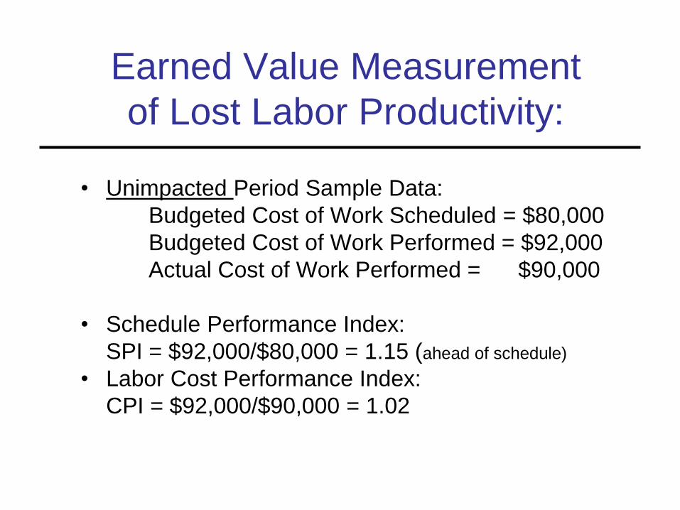
Earned Value Measurement
of Lost Labor Productivity:
• Unimpacted Period Sample Data:
Budgeted Cost of Work Scheduled = $80,000
Budgeted Cost of Work Performed = $92,000
Actual Cost of Work Performed = $90,000
• Schedule Performance Index:
SPI = $92,000/$80,000 = 1.15 (ahead of schedule)
• Labor Cost Performance Index:
CPI = $92,000/$90,000 = 1.02
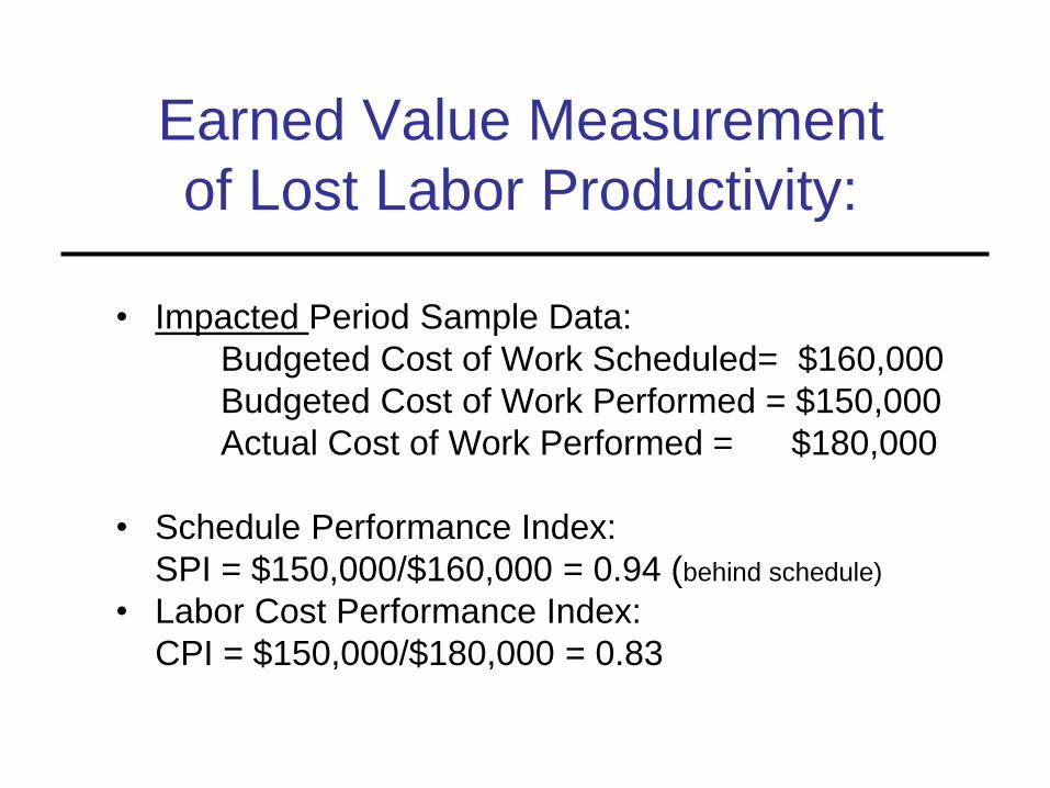
Earned Value Measurement
of Lost Labor Productivity:
• Impacted Period Sample Data:
Budgeted Cost of Work Scheduled= $160,000
Budgeted Cost of Work Performed = $150,000
Actual Cost of Work Performed = $180,000
• Schedule Performance Index:
SPI = $150,000/$160,000 = 0.94 (behind schedule)
• Labor Cost Performance Index:
CPI = $150,000/$180,000 = 0.83
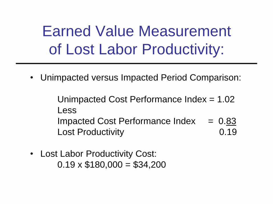
Earned Value Measurement
of Lost Labor Productivity:
• Unimpacted versus Impacted Period Comparison:
Unimpacted Cost Performance Index = 1.02
Less
Impacted Cost Performance Index = 0.83
Lost Productivity 0.19
• Lost Labor Productivity Cost:
0.19 x $180,000 = $34,200
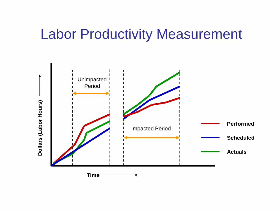
Labor Productivity Measurement
Time
Do
lla
rs (
La
bo
r H
ou
rs)
Performed
Scheduled
Actuals
Unimpacted
Period
Impacted Period
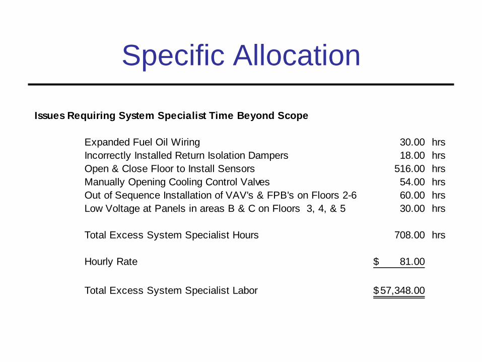
Specific Allocation
Issues Requiring System Specialist Time Beyond Scope
Expanded Fuel Oil Wiring 30.00 hrs
Incorrectly Installed Return Isolation Dampers 18.00 hrs
Open & Close Floor to Install Sensors 516.00 hrs
Manually Opening Cooling Control Valves 54.00 hrs
Out of Sequence Installation of VAV's & FPB's on Floors 2-6 60.00 hrs
Low Voltage at Panels in areas B & C on Floors 3, 4, & 5 30.00 hrs
Total Excess System Specialist Hours 708.00 hrs
Hourly Rate 81.00$
Total Excess System Specialist Labor 57,348.00$

Lost Productivity and
Efficiency
Ranking of Best Practices
AACE Recommended Practice
No. 25R-03
The Association for the Advancement of
Cost Engineering’s Recommended
Practice No. 25R-03 identifies lost
productivity estimating methodologies,
ranks the methodologies in order of
preference, defines and discusses each
methodology, and identifies selected
studies applicable to each methodology.
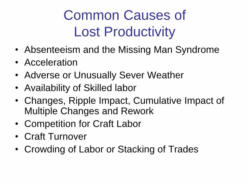
Common Causes of
Lost Productivity
• Absenteeism and the Missing Man Syndrome
• Acceleration
• Adverse or Unusually Sever Weather
• Availability of Skilled labor
• Changes, Ripple Impact, Cumulative Impact of Multiple Changes and Rework
• Competition for Craft Labor
• Craft Turnover
• Crowding of Labor or Stacking of Trades
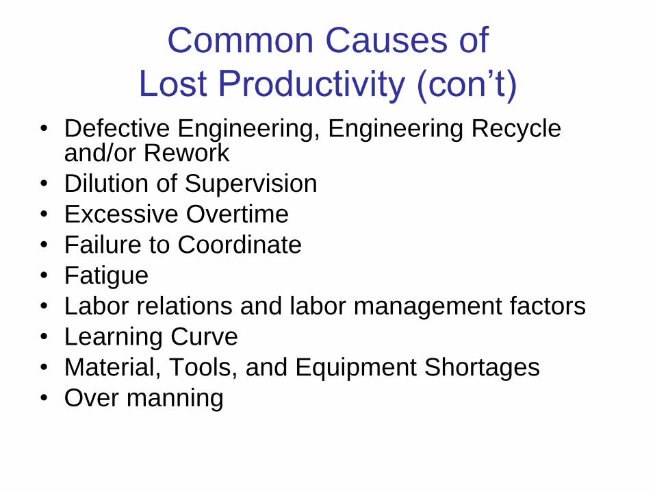
Common Causes of
Lost Productivity (con’t) • Defective Engineering, Engineering Recycle
and/or Rework
• Dilution of Supervision
• Excessive Overtime
• Failure to Coordinate
• Fatigue
• Labor relations and labor management factors
• Learning Curve
• Material, Tools, and Equipment Shortages
• Over manning
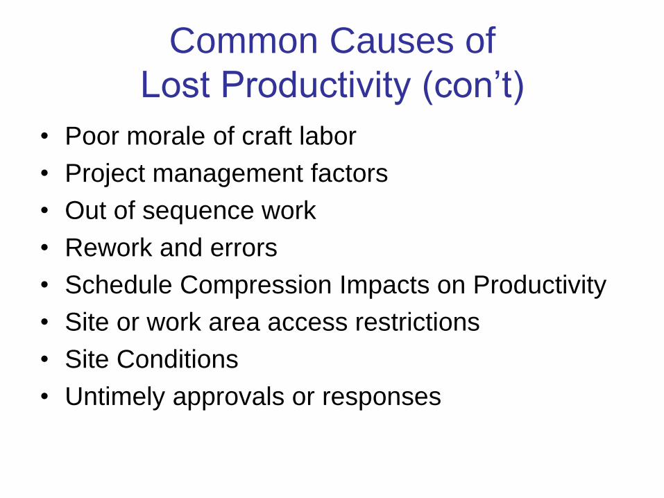
Common Causes of
Lost Productivity (con’t)
• Poor morale of craft labor
• Project management factors
• Out of sequence work
• Rework and errors
• Schedule Compression Impacts on Productivity
• Site or work area access restrictions
• Site Conditions
• Untimely approvals or responses
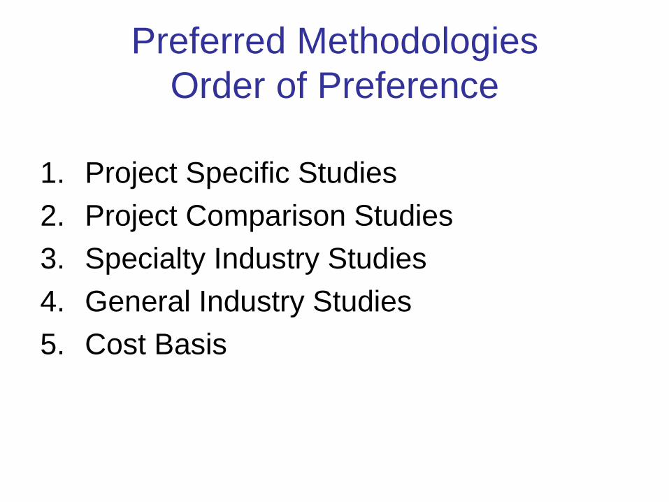
Preferred Methodologies
Order of Preference
1. Project Specific Studies
2. Project Comparison Studies
3. Specialty Industry Studies
4. General Industry Studies
5. Cost Basis
Project Specific Studies
Damage calculations based directly on
data from the project in dispute and
supported by contemporaneous
documentation are most favorably
received by courts and board of appeal.

Project Specific Studies
• Measured Mile Study
• Earned Value Analysis
• Work Sampling Method
• Craftsmen Questionnaire Sampling
Method
Work Sampling Method
The work sampling method involves the
claims analyst making numerous direct
observations of work activities.
Statistically valid sampling techniques are
used to determine how much time is spent
between direct work, support work and
delays/disruptions.

Craftsmen Questionnaire
Sampling Method This method involves preparing a
questionnaire and providing it to the craftsmen in the field during the lost productivity period.
The questionnaire allows the craftsmen to estimate the amount of lost productivity on a daily or weekly basis, identifying the causes of the lost time.

Project Comparison Studies
When there is insufficient contemporaneous
project documentation available to support
a Project Specific Study, AACE
recommends a Project Comparison study
as the next best alternative.
Project Comparison Studies
Comparable Work Study
Compares productivity of one work activity
to a similar work activity on the same
project.
Comparable Project Study
Compares productivity on one project to
productivity achieved on a similar project.

Specialty Industry Studies
When there is insufficient contemporaneous project documentation to allow for use of a Project Specific or Project Comparison study, AACE recommends use of an appropriate Specialty Industry study.
The primary differences between Specialty Industry Studies and General Industry studies are the Specialty studies are subject specific, limited to a specific industry, and based upon a small number of specific projects rather than a generalized survey of the industry.

Specialty Industry Studies
• Acceleration – Construction Industry Institute, CII Research Summary RS 41-1,
Schedule Reduction Executive Summary, Austin, Texas, April 1995
– NECA, Electrical Construction Peak Workforce Report, 2nd Edition, Washington D.C., 1987
• Changes, Cumulative Impact and Rework – Leonard, Charles A., The Effects of Change Orders on Productivity,
Concordia University, Montreal, Quebec, April 14, 1987
– Mechanical Contractors Association of America, Change Orders, Overtime and Productivity, Publication M3, Rockville, MD., 1968
• Learning Curve – Cass, Donald J., Labor Productivity Impact of Varying Crew Levels,
C.2.1, AACEI Transactions, 1992
– Emir, Zey, Learning Curve in Construction, Revay Reports, Vol. 18, No. 3, October 1999.

Specialty Industry Studies
• Overtime and Shift Work – Adrian, James J., Construction Productivity Improvement, Elsevier
Science Publishing, New York, 1987.
– Business Roundtable, Effect of Scheduled Overtime on Construction
Projects-coming to Grips with Some Major Problems in the Construction
Industry, New York, 1974.
• Project Characteristics – Construction Industry Institute, Engineering Productivity Measurement,
CII Research Summary RS156-1, Austin, TX, December 2001.
– Merrow, Edward W., Understanding the Outcome of Mega Projects: A
Quantitative Analysis of Very Large Civil Projects, March 1988.

Specialty Industry Studies
• Project Management – Chitester, David D., A Model for Analyzing Jobsite Productivity, C.3.1,
AACEI Transactions, 1992.
– Thomas, H. Randolph, Jr., Victor E. Sanvido and Steve R. Sanders,
Impact of Materials Management on Productivity, Journal of
Construction Engineering and Management, Vol.115, No. 3, Sep 1989.
• Weather – U.S. Army Cold region Research and Engineering Laboratory, Impact
of Climatic Conditions on Productivity, Hanover, N.H., 1987.
– National Electrical Contractors Association, The Effect of Temperature
on Productivity, Washington, D.C. 1974

General Industry Studies
In situations where there is insufficient
contemporaneous documentation to
support either a project specific or project
comparison study and the lost productivity
stems from numerous or non-specific
factors, the AACE recommended practice
is to utilize an appropriate General
Industry Study.

General Industry Studies
• U.S. Army Corps of Engineers, Modification Impact Evaluation Guide, EP 415-1-3, Department of the Army, Office of Chief of Engineers, Washington, D.C., July 1979
• Mechanical Contractor’s Association of America (MCAA), Labor Estimating Manual: Appendix B, Factors Effecting Productivity, Rockville, MD., August 1988.
• National Electrical Contractor’s Association (NECA), Manual of Labor Units, Bethesda, MD., 1976 and 2003.
Cost Basis
When there is insufficient documentation to support any of the previously discussed techniques, the AACE recommends employing one of the Cost Basis Methods.
However, contractors should bear in mind that there are significant legal hurdles to overcome for use of a cost basis methodology.
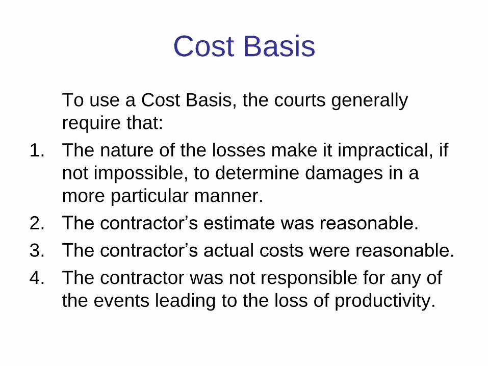
Cost Basis
To use a Cost Basis, the courts generally
require that:
1. The nature of the losses make it impractical, if
not impossible, to determine damages in a
more particular manner.
2. The contractor’s estimate was reasonable.
3. The contractor’s actual costs were reasonable.
4. The contractor was not responsible for any of
the events leading to the loss of productivity.
Cost Basis
• Total Unit Cost Method
• Modified Total Labor Cost Method
• Total Labor Cost Method
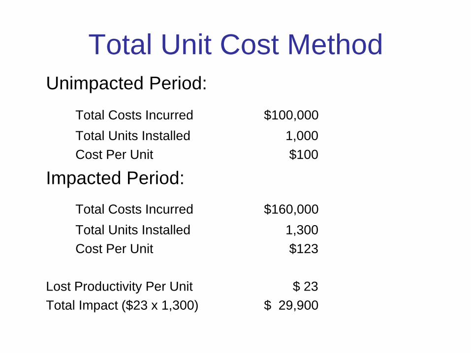
Total Unit Cost Method
Unimpacted Period:
Total Costs Incurred $100,000
Total Units Installed 1,000
Cost Per Unit $100
Impacted Period:
Total Costs Incurred $160,000
Total Units Installed 1,300
Cost Per Unit $123
Lost Productivity Per Unit $ 23
Total Impact ($23 x 1,300) $ 29,900
Lost Productivity And
Efficiency
Understanding Cumulative Impact
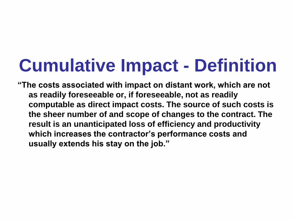
Cumulative Impact - Definition “The costs associated with impact on distant work, which are not
as readily foreseeable or, if foreseeable, not as readily
computable as direct impact costs. The source of such costs is
the sheer number of and scope of changes to the contract. The
result is an unanticipated loss of efficiency and productivity
which increases the contractor’s performance costs and
usually extends his stay on the job.”
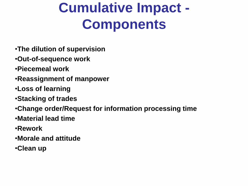
Cumulative Impact -
Components
•The dilution of supervision
•Out-of-sequence work
•Piecemeal work
•Reassignment of manpower
•Loss of learning
•Stacking of trades
•Change order/Request for information processing time
•Material lead time
•Rework
•Morale and attitude
•Clean up

Cumulative Impact –
Quantification • Methodology developed jointly by:
– Construction Industry Institute
– Electrical Contracting Foundation
– Mechanical Contracting Foundation

Cumulative Impact –
Quantification • First Step –
What is the probability of being affected?
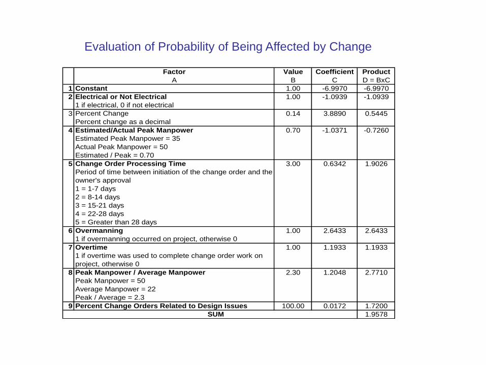
Evaluation of Probability of Being Affected by Change
Factor Value Coefficient Product
A B C D = BxC
1 Constant 1.00 -6.9970 -6.9970
2 Electrical or Not Electrical 1.00 -1.0939 -1.0939
1 if electrical, 0 if not electrical
3 Percent Change 0.14 3.8890 0.5445
Percent change as a decimal
4 Estimated/Actual Peak Manpower 0.70 -1.0371 -0.7260
Estimated Peak Manpower = 35
Actual Peak Manpower = 50
Estimated / Peak = 0.70
5 Change Order Processing Time 3.00 0.6342 1.9026
Period of time between initiation of the change order and the
owner's approval
1 = 1-7 days
2 = 8-14 days
3 = 15-21 days
4 = 22-28 days
5 = Greater than 28 days
6 Overmanning 1.00 2.6433 2.6433
1 if overmanning occurred on project, otherwise 0
7 Overtime 1.00 1.1933 1.1933
1 if overtime was used to complete change order work on
project, otherwise 0
8 Peak Manpower / Average Manpower 2.30 1.2048 2.7710
Peak Manpower = 50
Average Manpower = 22
Peak / Average = 2.3
9 Percent Change Orders Related to Design Issues 100.00 0.0172 1.7200
SUM 1.9578
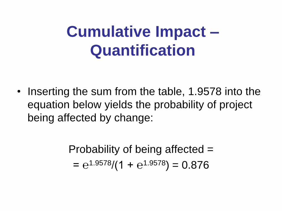
Cumulative Impact –
Quantification
• Inserting the sum from the table, 1.9578 into the
equation below yields the probability of project
being affected by change:
Probability of being affected =
= ℮1.9578/(1 + ℮1.9578) = 0.876
Cumulative Impact –
Quantification
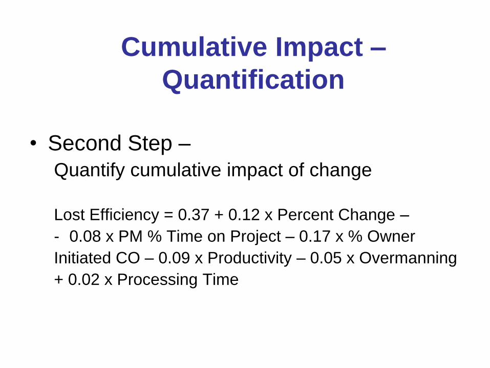
• Second Step –
Quantify cumulative impact of change
Lost Efficiency = 0.37 + 0.12 x Percent Change –
- 0.08 x PM % Time on Project – 0.17 x % Owner
Initiated CO – 0.09 x Productivity – 0.05 x Overmanning
+ 0.02 x Processing Time
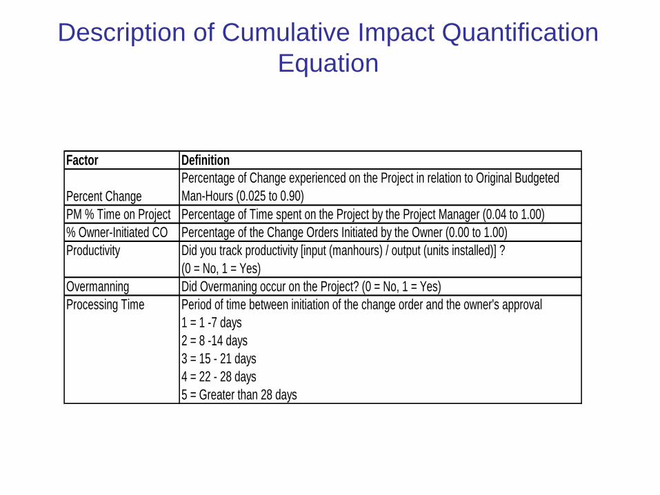
Description of Cumulative Impact Quantification
Equation
Factor Definition
Percent Change
Percentage of Change experienced on the Project in relation to Original Budgeted
Man-Hours (0.025 to 0.90)
PM % Time on Project Percentage of Time spent on the Project by the Project Manager (0.04 to 1.00)
% Owner-Initiated CO Percentage of the Change Orders Initiated by the Owner (0.00 to 1.00)
Productivity Did you track productivity [input (manhours) / output (units installed)] ?
(0 = No, 1 = Yes)
Overmanning Did Overmaning occur on the Project? (0 = No, 1 = Yes)
Processing Time Period of time between initiation of the change order and the owner's approval
1 = 1 -7 days
2 = 8 -14 days
3 = 15 - 21 days
4 = 22 - 28 days
5 = Greater than 28 days
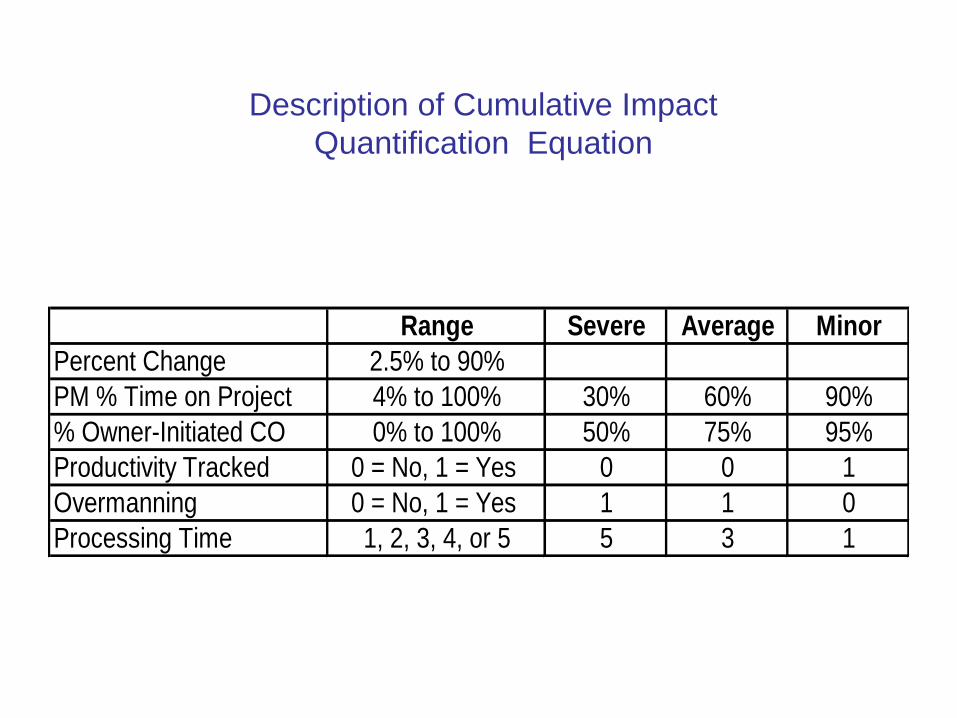
Description of Cumulative Impact
Quantification Equation
Range Severe Average Minor
Percent Change 2.5% to 90%
PM % Time on Project 4% to 100% 30% 60% 90%
% Owner-Initiated CO 0% to 100% 50% 75% 95%
Productivity Tracked 0 = No, 1 = Yes 0 0 1
Overmanning 0 = No, 1 = Yes 1 1 0
Processing Time 1, 2, 3, 4, or 5 5 3 1
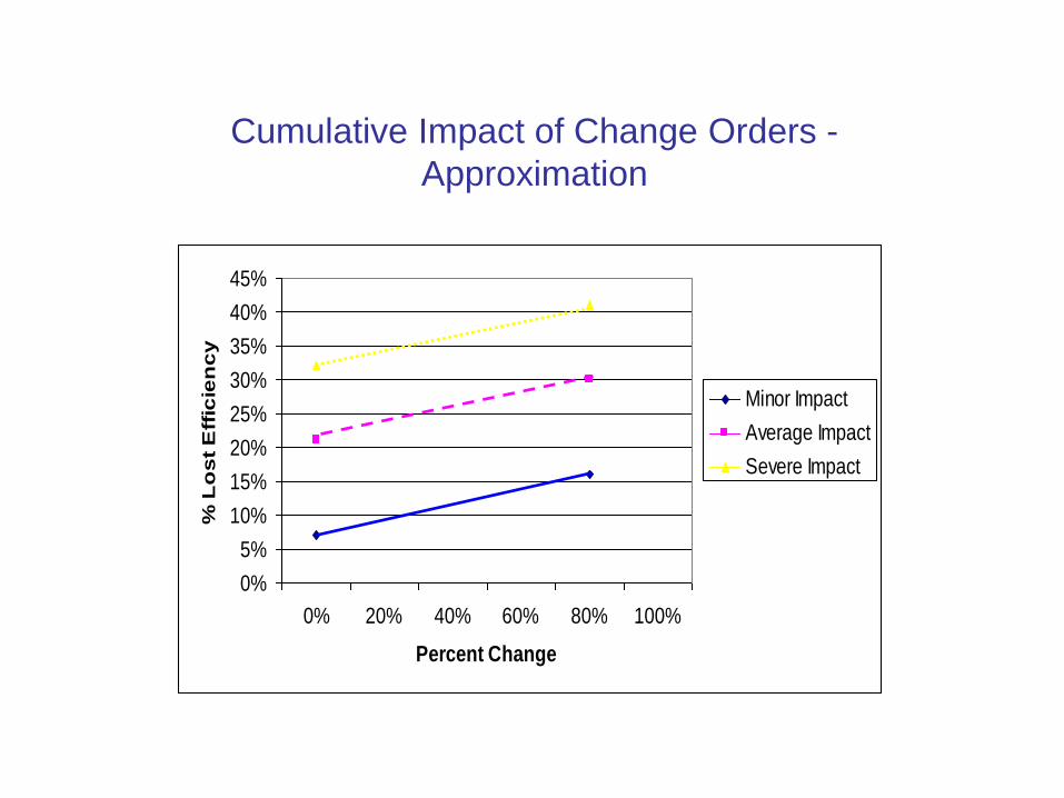
Cumulative Impact of Change Orders -
Approximation
0%
5%
10%
15%
20%
25%
30%
35%
40%
45%
0% 20% 40% 60% 80% 100%
Percent Change
% L
os
t E
ffic
ien
cy
Minor Impact
Average Impact
Severe Impact
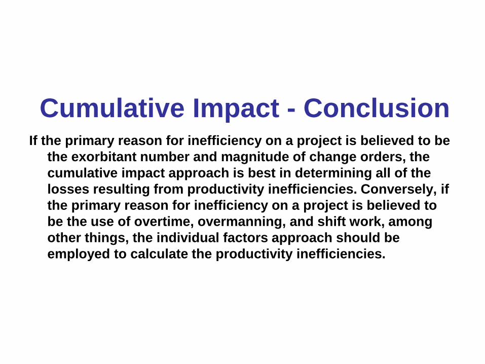
Cumulative Impact - Conclusion If the primary reason for inefficiency on a project is believed to be
the exorbitant number and magnitude of change orders, the
cumulative impact approach is best in determining all of the
losses resulting from productivity inefficiencies. Conversely, if
the primary reason for inefficiency on a project is believed to
be the use of overtime, overmanning, and shift work, among
other things, the individual factors approach should be
employed to calculate the productivity inefficiencies.
Lost Productivity And
Efficiency
Recovery of Home Office Overhead

Home Office Overhead Defined
A Home Office exists to run a business and to support all the projects in progress. Its costs are real, but are not directly associated with a particular project
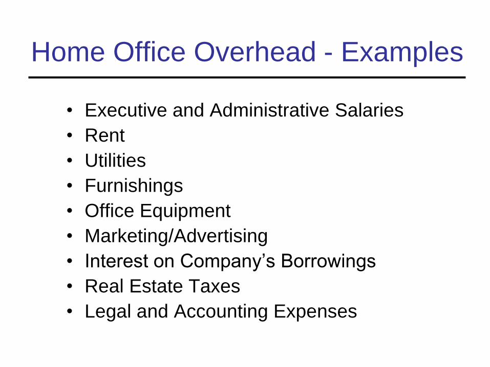
Home Office Overhead - Examples
• Executive and Administrative Salaries
• Rent
• Utilities
• Furnishings
• Office Equipment
• Marketing/Advertising
• Interest on Company’s Borrowings
• Real Estate Taxes
• Legal and Accounting Expenses
Profitability Formula
Project Revenue
Less:
– Direct Cost
– Field Overhead
– Home Office Overhead
Equals: Profit

Home Office
Overhead Absorption
• 1 Project Example
– When a contractor
performs one project
at a time, that project
needs to pay for
(absorb) 100% of
Home Office Cost
Percentage of Home Office
Overhead Absorbed by
1 Project
100%
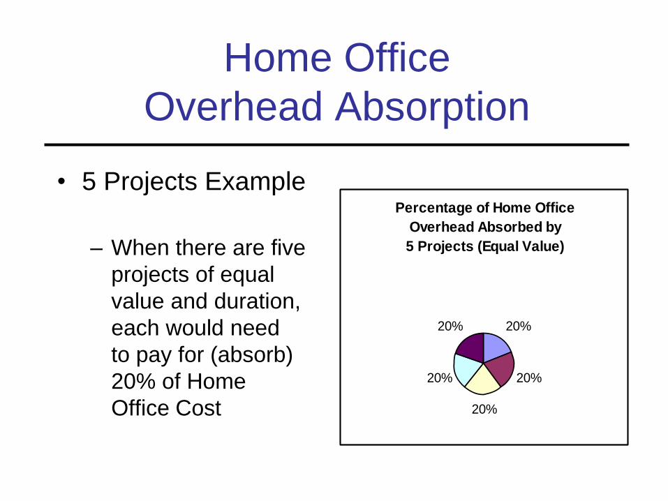
• 5 Projects Example
– When there are five
projects of equal
value and duration,
each would need
to pay for (absorb)
20% of Home
Office Cost
Percentage of Home Office
Overhead Absorbed by
5 Projects (Equal Value)
20%
20%
20%
20%
20%
Home Office
Overhead Absorption
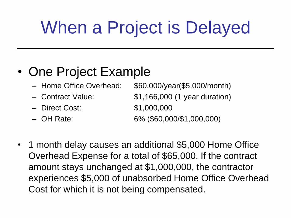
When a Project is Delayed
• One Project Example – Home Office Overhead: $60,000/year($5,000/month)
– Contract Value: $1,166,000 (1 year duration)
– Direct Cost: $1,000,000
– OH Rate: 6% ($60,000/$1,000,000)
• 1 month delay causes an additional $5,000 Home Office
Overhead Expense for a total of $65,000. If the contract
amount stays unchanged at $1,000,000, the contractor
experiences $5,000 of unabsorbed Home Office Overhead
Cost for which it is not being compensated.
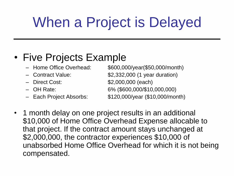
When a Project is Delayed
• Five Projects Example – Home Office Overhead: $600,000/year($50,000/month)
– Contract Value: $2,332,000 (1 year duration)
– Direct Cost: $2,000,000 (each)
– OH Rate: 6% ($600,000/$10,000,000)
– Each Project Absorbs: $120,000/year ($10,000/month)
• 1 month delay on one project results in an additional $10,000 of Home Office Overhead Expense allocable to that project. If the contract amount stays unchanged at $2,000,000, the contractor experiences $10,000 of unabsorbed Home Office Overhead for which it is not being compensated.
• Reality Check
– Multiple Projects
– Varying Direct Costs
– Range of Durations
– Varying level of Home Office Support
• Overhead Rates computed using historical data are applied to future projects
Home Office
Overhead Absorption
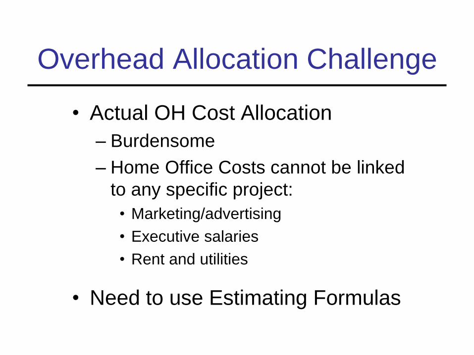
Overhead Allocation Challenge
• Actual OH Cost Allocation
– Burdensome
– Home Office Costs cannot be linked
to any specific project:
• Marketing/advertising
• Executive salaries
• Rent and utilities
• Need to use Estimating Formulas
Eichleay Formula
• Most widely accepted
– Federal Courts
– Numerous state courts
– Private arbitration
• Originated in 1960 from an Armed
Services Board of Contract Appeals
Decision.
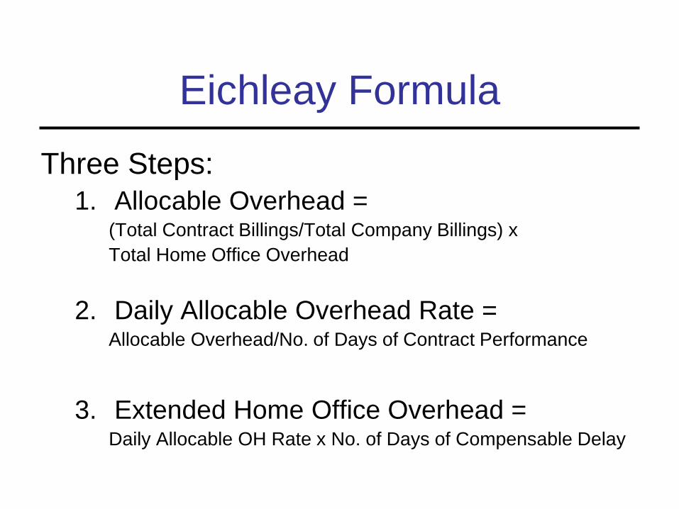
Eichleay Formula
Three Steps:
1. Allocable Overhead = (Total Contract Billings/Total Company Billings) x
Total Home Office Overhead
2. Daily Allocable Overhead Rate = Allocable Overhead/No. of Days of Contract Performance
3. Extended Home Office Overhead = Daily Allocable OH Rate x No. of Days of Compensable Delay
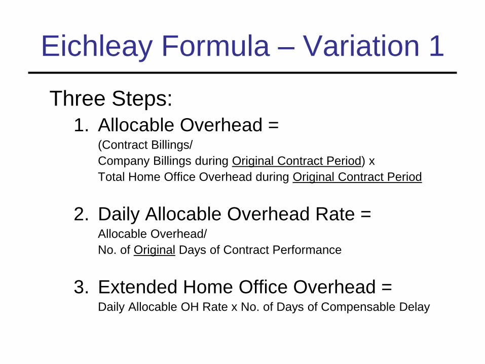
Eichleay Formula – Variation 1
Three Steps:
1. Allocable Overhead = (Contract Billings/
Company Billings during Original Contract Period) x
Total Home Office Overhead during Original Contract Period
2. Daily Allocable Overhead Rate = Allocable Overhead/
No. of Original Days of Contract Performance
3. Extended Home Office Overhead = Daily Allocable OH Rate x No. of Days of Compensable Delay
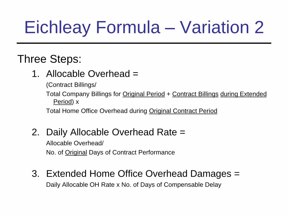
Eichleay Formula – Variation 2
Three Steps:
1. Allocable Overhead = (Contract Billings/
Total Company Billings for Original Period + Contract Billings during Extended
Period) x
Total Home Office Overhead during Original Contract Period
2. Daily Allocable Overhead Rate = Allocable Overhead/
No. of Original Days of Contract Performance
3. Extended Home Office Overhead Damages = Daily Allocable OH Rate x No. of Days of Compensable Delay
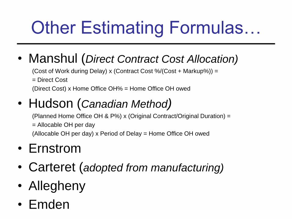
Other Estimating Formulas…
• Manshul (Direct Contract Cost Allocation) (Cost of Work during Delay) x (Contract Cost %/(Cost + Markup%)) =
= Direct Cost
(Direct Cost) x Home Office OH% = Home Office OH owed
• Hudson (Canadian Method) (Planned Home Office OH & P%) x (Original Contract/Original Duration) =
= Allocable OH per day
(Allocable OH per day) x Period of Delay = Home Office OH owed
• Ernstrom
• Carteret (adopted from manufacturing)
• Allegheny
• Emden
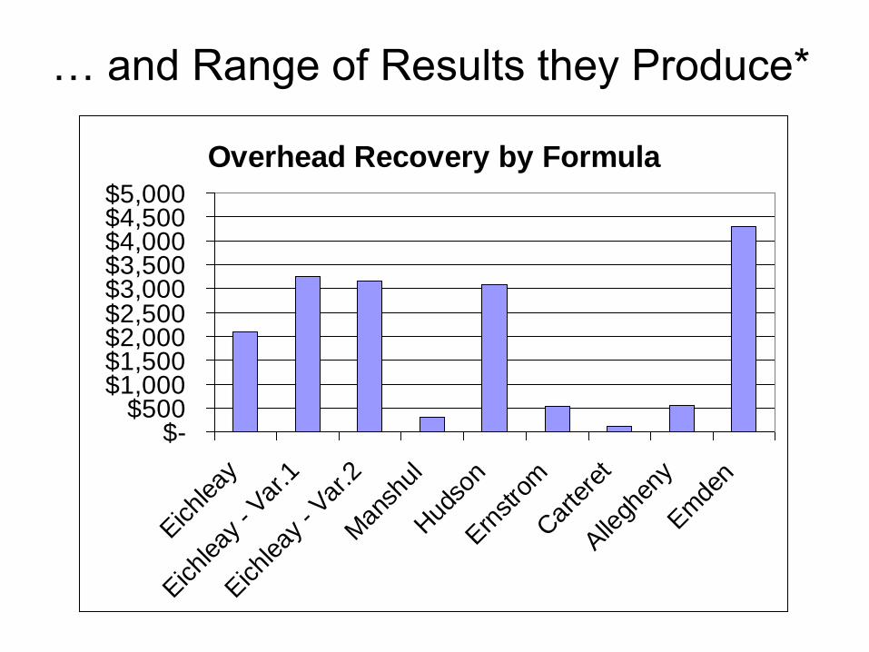
… and Range of Results they Produce*
Overhead Recovery by Formula
$-$500
$1,000$1,500$2,000$2,500$3,000$3,500$4,000$4,500$5,000
Eichlea
y
Eichlea
y - V
ar.1
Eichlea
y - V
ar.2
Man
shul
Hud
son
Ern
stro
m
Car
tere
t
Alle
ghen
y
Em
den
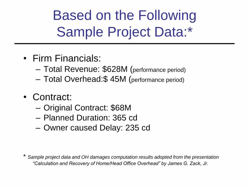
Based on the Following
Sample Project Data:*
• Firm Financials: – Total Revenue: $628M (performance period)
– Total Overhead:$ 45M (performance period)
• Contract: – Original Contract: $68M
– Planned Duration: 365 cd
– Owner caused Delay: 235 cd
* Sample project data and OH damages computation results adopted from the presentation
“Calculation and Recovery of Home/Head Office Overhead” by James G. Zack, Jr.
Entitlement – Raising the Bar
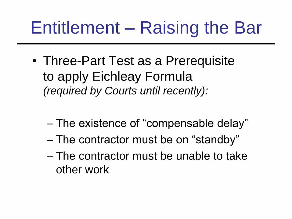
• Three-Part Test as a Prerequisite
to apply Eichleay Formula (required by Courts until recently):
– The existence of “compensable delay”
– The contractor must be on “standby”
– The contractor must be unable to take
other work
Entitlement – Raising the Bar
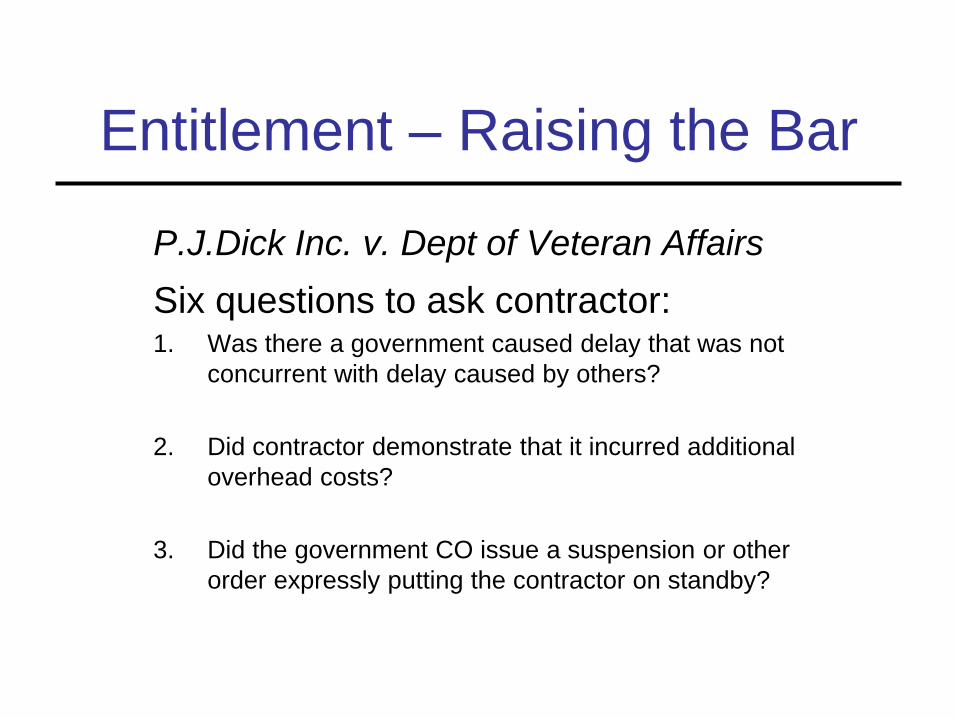
P.J.Dick Inc. v. Dept of Veteran Affairs
Six questions to ask contractor: 1. Was there a government caused delay that was not
concurrent with delay caused by others?
2. Did contractor demonstrate that it incurred additional
overhead costs?
3. Did the government CO issue a suspension or other
order expressly putting the contractor on standby?
Entitlement – Raising the Bar
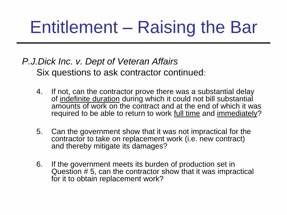
P.J.Dick Inc. v. Dept of Veteran Affairs
Six questions to ask contractor continued:
4. If not, can the contractor prove there was a substantial delay of indefinite duration during which it could not bill substantial amounts of work on the contract and at the end of which it was required to be able to return to work full time and immediately?
5. Can the government show that it was not impractical for the contractor to take on replacement work (i.e. new contract) and thereby mitigate its damages?
6. If the government meets its burden of production set in Question # 5, can the contractor show that it was impractical for it to obtain replacement work?
Entitlement – Raising the Bar
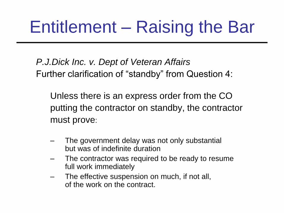
P.J.Dick Inc. v. Dept of Veteran Affairs
Further clarification of “standby” from Question 4:
Unless there is an express order from the CO
putting the contractor on standby, the contractor
must prove:
– The government delay was not only substantial but was of indefinite duration
– The contractor was required to be ready to resume full work immediately
– The effective suspension on much, if not all, of the work on the contract.
Entitlement – Controversial Points
• The difference between “suspension” period versus “delay” period.
– “suspension” does not automatically lead to extension of time.
• The power of the “no damage for delay” clause; can it prevent recovery under Eichleay?
Entitlement – Controversial Points
• “Credits” are due when:
– The contractor performs change order work that provides for some extension of time
– The contractor re-assigns some of its work force to perform replacement work
Practical Suggestions
• Document planned schedules
• Document the cause of the delay, including factors adding to its uncertainty
• Document efforts to obtain replacement work – If successful, maintain separate accounting of this
work to compute the amount of “absorbed” overhead
• Build in a compensation for Extended Home Office OH into the contract language