CHANGE ORDERS AND PRODUCTIVITY LOSS QUANTIFICATION

CHANGE ORDERS AND PRODUCTIVITY LOSS QUANTIFICATION USING VERIFIABLE SITE DATA

by

ENGY SERAG B.S. The American University In Cairo, 2000 M.S. The American University In Cairo, 2003

A dissertation submitted in partial fulfillment of the requirements for the degree of Doctor of Philosophy

in the Department of Civil and Environmental Engineering in the College of Engineering and Computer Science

at the University of Central Florida Orlando, Florida

Summer Term 2006

Major Professor: Amr Oloufa

ii

© 2006 Engy Serag

iii

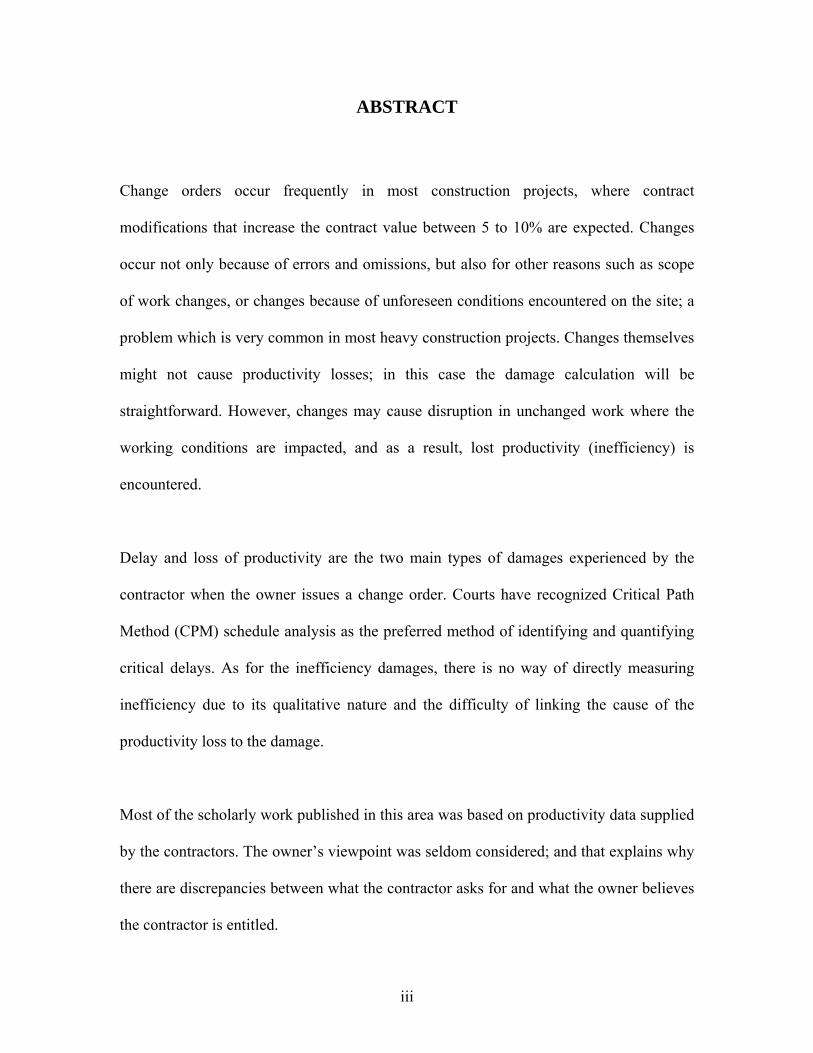
ABSTRACT

Change orders occur frequently in most construction projects, where contract

modifications that increase the contract value between 5 to 10% are expected. Changes

occur not only because of errors and omissions, but also for other reasons such as scope

of work changes, or changes because of unforeseen conditions encountered on the site; a

problem which is very common in most heavy construction projects. Changes themselves

might not cause productivity losses; in this case the damage calculation will be

straightforward. However, changes may cause disruption in unchanged work where the

working conditions are impacted, and as a result, lost productivity (inefficiency) is

encountered.

Delay and loss of productivity are the two main types of damages experienced by the

contractor when the owner issues a change order. Courts have recognized Critical Path

Method (CPM) schedule analysis as the preferred method of identifying and quantifying

critical delays. As for the inefficiency damages, there is no way of directly measuring

inefficiency due to its qualitative nature and the difficulty of linking the cause of the

productivity loss to the damage.

Most of the scholarly work published in this area was based on productivity data supplied

by the contractors. The owner’s viewpoint was seldom considered; and that explains why

there are discrepancies between what the contractor asks for and what the owner believes

the contractor is entitled.

iv

This research focuses on analyzing the change orders and the productivity loss from

public owner data. The study addresses the need for a statistical model to quantify the

change orders and the productivity loss from verifiable owner’s data such as owner’s

daily reports, change orders, drawing, and specifications, rather than rely on contractor

surveys.

Two models are developed and validated; the first model is to quantify the percent

increase in the contract price due to the change orders. This model will provide the owner

with an estimate of the cost of the changed work, where it can be used for forward pricing

or retrospective pricing of the change orders. The second is to quantify the productivity

loss of the piping work due to the change orders. The productivity loss study analyzed

two set of data; the first included all the predictor variables which both parties, the owner

and the contractor, contributed to the productivity loss, and the second one included the

predictor variables, from the legal view point, only the owner is responsible for. The

study showed the difference between what the contractor asked for and what he is

actually entitled. This model can be used by both the owner and the contractor to

quantify the productivity loss due to change orders.

v

ACKNOWLEDGMENTS

First I would like to thank God for the blessings granted to me all the way till I finish this

work, and all through my life.

I would like to express my gratitude to my professor Dr Amr Oloufa for his support and

guidance since I started my doctoral. He taught me how to be a great instructor, a

distinguished researcher and a giving person. I really owe him every successful step I

achieved since I started here.

I would like to thank my committee members Dr Essam Radwan, Dr Linda Malone, Dr

Shiou-San Kuo , and Dr Sastry Putcha for the time they spent with me to guide me to the

right research directions.

I would like to thank Florida Department of Transportation for their great help in

providing me with the data needed to conduct this research. Also, Florida Department of

Transportation claims consultants who guided me to the problem areas that need to be

further studied in heavy construction projects.

Last or I can say, right after God, my parents, they have been a great support by traveling

all the way to be beside me and give me a push to work hard. And now I have fulfilled

their dream and my dream and without the love, support and encouragement they gave

me, I wouldn’t have been writing this dissertation.

vi

TABLE OF CONTENTS

LIST OF FIGURES ............................................................................................................ x

LIST OF TABLES............................................................................................................ xii

CHAPTER 1: INTRODUCTION....................................................................................... 1

1.1 Background............................................................................................................. 1

1.2 Productive vs. Non-Productive labor...................................................................... 2 1.2.1 Industry Related Factors ................................................................................. 3 1.2.2 Labor Related Factors ..................................................................................... 5 1.2.3 Management Related Factors.......................................................................... 6

1.3 How Changes Cause Loss of Productivity.............................................................. 6

1.4 Labor Productivity Inefficiency.............................................................................. 7

1.5 Measuring Inefficiency ......................................................................................... 11

1.6 Problem Statement ................................................................................................ 13

1.7 Research Objective ............................................................................................... 14

1.8 Research Methodology ......................................................................................... 15

1.9 Scope of Work ...................................................................................................... 18

1.10 Summary ............................................................................................................... 19

CHAPTER 2: LITERATURE REVIEW.......................................................................... 21

2.1 Introduction........................................................................................................... 21

2.2 Methods of Measuring Inefficiency...................................................................... 24 2.2.1 Total Cost Method ........................................................................................ 24 2.2.2 Modified Total Cost Method ........................................................................ 25 2.2.3 Industry Standards ........................................................................................ 26

2.2.3.1 U.S. Army Corps of Engineers ................................................................. 26

2.2.3.2 National Electrical Contractors Association (NECA) .............................. 27

2.2.3.3 Mechanical Contractors Association of America (MCAA)...................... 29

vii

2.2.4 Learning Curve ............................................................................................. 32 2.2.5 Measured Mile Approach ............................................................................. 35

2.2.5.1 Sources of Extracting Data to Use Measured Mile................................... 36

2.2.5.2 Proof of Causation .................................................................................... 38

2.2.5.3 Measured Mile Process ............................................................................. 39

2.2.5.4 Measured Mile Advantages ...................................................................... 40

2.2.5.5 Measured Mile Limitations....................................................................... 40

2.2.6 Baseline Productivity .................................................................................... 41 2.2.6.1 Thomas Approach..................................................................................... 42

2.2.6.2 Control Charts........................................................................................... 46

2.2.7 Statistical Approaches................................................................................... 49 2.2.7.1 Leonard Study........................................................................................... 49

2.2.7.2 Construction Industry Institute Study ....................................................... 51

2.2.7.3 Thomas Approach..................................................................................... 52

2.2.7.4 % Delta Approach (Hanna, 1999a, b)....................................................... 56

2.2.7.5 Decision Tree (Lee, 2004) ........................................................................ 66

2.2.8 Neural Network............................................................................................. 69

2.3 Summary ............................................................................................................... 74

CHAPTER 3: METHODOLOGY .................................................................................... 75

3.1 Background........................................................................................................... 75

3.2 Data Collection ..................................................................................................... 75

3.3 Data Preparation.................................................................................................... 77 3.3.1 Change Order Study...................................................................................... 78

3.3.1.1 Dependant Variable (Response): .............................................................. 78

3.3.1.2 Predictor Variables.................................................................................... 79

3.3.2 Loss of Productivity Study............................................................................ 89 3.3.2.1 Introduction............................................................................................... 89

3.3.2.2 Dependant Variable .................................................................................. 93

3.3.2.3 Predictor Variables.................................................................................... 94

3.4 Model Development............................................................................................ 104 3.4.1 Need for a Simple Model............................................................................ 104 3.4.2 Too Many Variables ................................................................................... 105

viii

3.4.2.1 Interaction Variables............................................................................... 106

3.4.2.2 Multicollinearity Problem with Too Many Variables............................. 118

3.4.3 Scatter Plots ................................................................................................ 119

3.5 Hypothesis Testing.............................................................................................. 120 3.5.1 Multiple Regression.................................................................................... 120

3.6 Model Building Procedures ................................................................................ 121

3.7 Assessing Model Adequacy:............................................................................... 125

3.8 Multiple Regression Assumption........................................................................ 125 3.8.1 Variable Transformation............................................................................. 127

3.9 Model Validation ................................................................................................ 129

CHAPTER 4: RESULTS & ANALYSIS....................................................................... 131

4.1 Background......................................................................................................... 131

4.2 Data Exploration Stage ....................................................................................... 131 4.2.1 Data Range.................................................................................................. 133

4.2.1.1 Change Order Model............................................................................... 133

4.2.1.2 Piping Model........................................................................................... 159

4.2.2 Data Visualization....................................................................................... 190

4.3 Model Building ................................................................................................... 195 4.3.1 Model without Interaction........................................................................... 195

4.3.1.1 Change Order Model............................................................................... 195

4.3.1.2 Piping Model........................................................................................... 197

4.3.2 Model with Interaction................................................................................ 199 4.3.2.1 Change Order (Total Model) .................................................................. 199

4.3.2.2 Change Order Model for Percent Increase More Than 5% .................... 204

4.3.2.3 Change Order Model for Percent Increase Less than 5%....................... 209

4.3.2.4 Piping Model (Total Model) ................................................................... 212

4.3.2.5 Piping Model for PRLOSS>0% Suffered by the Contractor:................. 215

4.3.2.6 Piping Model for PRLOSS>0% Legal View Point ................................ 220

4.4 Model Validation ................................................................................................ 224 4.4.1 Change Order Model PERCINC >5% ........................................................ 225 4.4.2 Change order Model PERCINC<5%.......................................................... 227

ix

4.4.3 Piping Model with PRLOSS >0% Suffered by the Contractor .................. 228 4.4.4 Piping Model with PRLOSS >0% Legal View Point ................................. 229

4.5 Model Implementation........................................................................................ 230 4.5.1 Introduction................................................................................................. 230 4.5.2 Loss of Productivity Case Study................................................................. 230

4.5.2.1 Loss of Productivity: Practical Application............................................ 236

4.5.3 Change Order Case Study........................................................................... 237

CHAPTER 5: CONCLUSION ....................................................................................... 242

5.1 Introduction......................................................................................................... 242

5.2 Research Strength ............................................................................................... 243

5.3 Major Findings.................................................................................................... 247 5.3.1 Change Order Study.................................................................................... 247 5.3.2 Loss of Productivity Study.......................................................................... 251

5.4 Research Contributions....................................................................................... 255

5.5 Future Work ........................................................................................................ 256

APPENDIX A: MCAA FACTORS................................................................................ 259

APPENDIX B: INDEPENDENT VARIABLES FOR TREE MODEL, LEE 2004 ...... 263

APPENDIX C: A SAMPLE OF THE INPUT DATA.................................................... 267

LIST OF REFERNCES .................................................................................................. 272

x

LIST OF FIGURES

Figure 1: NECA Overtime Chart (NECA, 1969).............................................................. 28 Figure 2: Hyperbolic Learning Curve (Wideman, 1994).................................................. 33 Figure 3: Straight Line Learning Curve (Wideman, 1994)............................................... 33 Figure 4: Learning Curve Equation Elaboration (Wideman, 1994) ................................. 34 Figure 5: Measured Mile Approach (Gulezian and Samelian, 2003) .............................. 38 Figure 6: Basic Control Chart Structure (Gulezian and Samelian, 2003)......................... 47 Figure 7: Results of Leonard Study (1987)....................................................................... 50 Figure 8: Graphical Illustration of Delta (Hanna, 1999b)................................................. 57 Figure 9: Planned and Actual Loading Curves (Hanna, 1999b)....................................... 58 Figure 10: Impact Classification Tree (Lee, 2004)........................................................... 67 Figure 11: Quantification Tree model (Lee, 2004)........................................................... 68 Figure 12: Data Collection Procedures ............................................................................. 77 Figure 13: Predictor Variables for Change Order Study .................................................. 80 Figure 14: Piping Activities (A J Mccormack & Son, 2006) ........................................... 91 Figure 15: Drainage Plan (FDOT) .................................................................................... 91 Figure 16: Predictor Variables for Productivity Loss Model............................................ 95 Figure 17: Change Order Model Interaction................................................................... 110 Figure 18: Productivity Loss Model Interaction............................................................. 111 Figure 19: Model Building Procedures........................................................................... 124 Figure 20: Unequal Variance (Habing, 2004)................................................................. 128 Figure 21: Lack of Linearity (Habing, 2004).................................................................. 129 Figure 22: Multi Plot Node (SAS):................................................................................. 133 Figure 23: Distribution of the Response Variable "PERCINC" in %............................. 134 Figure 24: Frequency of Time Factor in %..................................................................... 136 Figure 25: Time in % vs. % Increase.............................................................................. 137 Figure 26: Frequency of Reason Factor.......................................................................... 140 Figure 27: Reason vs. % Increase ................................................................................... 141 Figure 28: Frequency of Party Factor ............................................................................. 142 Figure 29: Party vs. % Increase ...................................................................................... 143 Figure 30: Frequency of Approved Change Order Hours in % Factor........................... 144 Figure 31: Approved Change Order Hours in % vs. % Increase .................................... 145 Figure 32: Frequency of Work Stoppage Factor............................................................. 146 Figure 33: Work Stoppage vs. % Increase...................................................................... 147 Figure 34: Frequency of Restricted Access Factor ......................................................... 148 Figure 35: Restricted Access vs. % Increase .................................................................. 148 Figure 36: Frequency of the Way Change Order Expended Factor................................ 150 Figure 37: Way Change Order Expended vs. % Increase............................................... 151 Figure 38: Rework Process (Robinson, 2003) ................................................................ 151 Figure 39: Frequency of the Way Change Order Compensated Factor.......................... 153 Figure 40: Way Change Order Compensated vs. % Increase......................................... 153 Figure 41: Frequency of Extension Factor in % ............................................................. 155 Figure 42: Extension vs. % Increase............................................................................... 155 Figure 43: Frequency of Season Factor .......................................................................... 157

xi

Figure 44: Season vs. % Increase ................................................................................... 157 Figure 45: Frequency of Stacking of Trade Factor......................................................... 158 Figure 46: Stacking of Trade vs. % Increase .................................................................. 159 Figure 47: Distribution of the Response Variable "PRLOSS" ....................................... 161 Figure 48: Frequency of Time Factor in %..................................................................... 162 Figure 49: Time in % vs. % Productivity Loss............................................................... 163 Figure 50: Frequency of Rain Factor .............................................................................. 164 Figure 51: Rain vs. % Productivity Loss ........................................................................ 165 Figure 52: Frequency of Dewatering Factor................................................................... 166 Figure 53: Dewatering vs. % Productivity Loss ............................................................. 167 Figure 54: Frequency of Conflict Factor ........................................................................ 168 Figure 55: Conflict vs. % Productivity Loss................................................................... 168 Figure 56: Frequency of Rework Factor (in %).............................................................. 170 Figure 57: Rework vs. % Productivity Loss ................................................................... 170 Figure 58: Frequency of % Quantity Installed................................................................ 172 Figure 59: %Quantity Installed vs. % Productivity Loss................................................ 173 Figure 60: Frequency of Trench Box Factor................................................................... 174 Figure 61: Trench Box vs. % Productivity Loss............................................................. 175 Figure 62: Frequency of Pipe Diameter Factor............................................................... 176 Figure 63: Pipe Diameter vs. % Productivity Loss......................................................... 177 Figure 64: Types of Stone Bedding (A J Mccormack & Son, 2006).............................. 178 Figure 65: Frequency of Pipe Type Factor ..................................................................... 179 Figure 66: Pipe Type vs. % Productivity Loss ............................................................... 180 Figure 67: Frequency of Start of Work Factor................................................................ 181 Figure 68: Start of Work vs. % Productivity Loss.......................................................... 182 Figure 69: Frequency of Location Factor ....................................................................... 183 Figure 70: Location vs. Productivity Loss...................................................................... 183 Figure 71: Frequency of the Design Factor .................................................................... 185 Figure 72: Design vs. % Productivity Loss .................................................................... 186 Figure 73: Frequency of Material Factor ........................................................................ 187 Figure 74: Material vs. % Productivity Loss .................................................................. 188 Figure 75: Frequency of Accident Factor ....................................................................... 189 Figure 76: Accident vs. % Productivity Loss ................................................................. 189 Figure 77: Scatter Plot of Time vs. % Increase .............................................................. 191 Figure 78: Scatter Plot of Party vs. % Increase .............................................................. 192 Figure 79: Scatter Plot of Time vs. % Productivity Loss ............................................... 193 Figure 80: Scatter Plot of Rain during Work vs. % Productivity Loss........................... 194 Figure 81: Scatter Plot of Dewatering vs. % Productivity Loss ..................................... 194 Figure 82: Residual Plots for PERCINC (Total Model)................................................. 203 Figure 83: Residual Plots for PERCINC >5%................................................................ 208 Figure 84: Residual Plot for PERCINC<5% .................................................................. 212 Figure 85: Residual Plot for PRLOSS (Total Model)..................................................... 215 Figure 86: Residual Plot for PRLOSS>0% Suffered by the Contractor......................... 220 Figure 87: Residual Plot for PRLOSS>0% Legal View Point ....................................... 224

xii

LIST OF TABLES

Table 1: Acceleration Approaches (Thomas & Oloufa, 1996) ........................................... 9 Table 2: Results of 1962 NECA Survey ........................................................................... 27 Table 3: Learning Curve in Productivity Estimation (Wideman, 1994)........................... 35 Table 4: Differences between the Measured Mile and Baseline Period (Thomas, 2000). 42 Table 5: Proposed Work Content for Masonry Database (Thomas, 1999)....................... 45 Table 6: Quantitative Effect of Disruption (Thomas, 1995b)........................................... 56 Table 7: Weighted Timing Example (Hanna, 1999b)....................................................... 61 Table 8: Coding Qualitative Variables ........................................................................... 112 Table 9: Change Order Model Variables ........................................................................ 113 Table 10: Piping Model Variables .................................................................................. 115 Table 11: Change Order Model without Interaction Variables ...................................... 196 Table 12: Piping Model without Interaction Variables................................................... 198 Table 13: Change Order Model with Interaction Variables (Total Model) .................... 201 Table 14: P-Values & VIF Change Order model for PERCINC >5% ........................... 207 Table 15: P-Values & VIF Change Order model for PERCINC <5% ........................... 211 Table 16: Piping Model with Interaction Variables (Total Model) ................................ 214 Table 17: P-Values for PRLOSS>0 Suffered by the Contractor .................................... 219 Table 18: P-Values for PRLOSS>0 Legal View Point................................................... 223 Table 19: Validation Data set for Change Order Model with PERCINC>5% ............... 226 Table 20: Validation Data set for Change Order Model with PERCINC<5% ............... 227 Table 21: Validation Data set for Piping Model with PRLOSS>0% Suffered by the Contractor ....................................................................................................................... 228 Table 22: Validation Data set for Piping Model with PRLOSS>0% Legal View Point 229 Table 23: Productivity Case Study Predictor Variables ................................................. 232 Table 24: Change Order Case Study Predictor Variables............................................... 239

Table A 1: MCAA Factors.............................................................................................. 260 Table A 2: Independent Variables for Tree Model, Lee 2004........................................ 264 Table A 3: Sample Data Input for Change Order Model with PERCINC >5% ............. 268 Table A 4: Sample Data Input for Change Order Model with PERCINC <5% ............. 269 Table A 5: Sample Data Input for Piping Model with PRLOSS>0% Suffered by the Contractor ....................................................................................................................... 270 Table A 6: Sample Data Input for Piping Model PRLOSS>0% Legal View Point ....... 271

1

CHAPTER 1: INTRODUCTION

1.1 Background

Change orders are frequently encountered in any construction project. Contract

modifications that increase the contract value from 5 to 10% are expected in most

construction projects (Finke, 1998a). The value of construction work put in place in

2003 was $ 870 billion (US Census Bureau). A 5% change rate on this $ 870 billion

means that just the direct costs of change approach $44 billion per year. In addition

there are other indirect costs such as higher insurance rates, delayed completion of

projects; and lost opportunity of bidding in other projects due to extended completion;

and so forth.

It is important to understand the types of costs in any construction projects to provide

a good estimate of the change costs. There are two types of costs in any construction

contract and they are fixed and variable costs. Fixed cost-items are the ones that the

contractor purchases on a fixed-price subcontract or purchase order. The risks

allocated in the fixed price are relatively low as the contractor has them fixed in the

agreement between him and the owner. The risks associated with the fixed cost-items

can be financial crisis, or a mistake done by the subcontractor that can lead to

defective work. The variable cost-items are items such as the labor, equipment and

overhead. The major variable risk item in any construction project is the labor as they

are frequently the most variable cost for the contractor. The main areas of labor cost

2

increase include schedule acceleration, changes in the scope of work, project

management, project location and external characteristics. Each of these areas has

main subcategories that can affect the labor cost. Schedule acceleration may lead to

overcrowding, stacking of trades, and overtime. Changes in the scope of work may

lead to additional quantities of material, learning curve changes, delays, engineering

errors and omissions, rework of already installed work, and changes to the plans and

specifications. As for the management characteristics, any deficiency in this area

might negatively affect the material and tool availability, the coordination between

the team members, and the effectiveness of the supervision. Project location and

external conditions include weather, altitude, availability of skilled labor and the

economic market in the area where the project is constructed (Shawartzkoph, 1995).

1.2 Productive vs. Non-Productive labor

Productivity is the units of work accomplished for the units of labor expended in such

work. The U.S. Department of Commerce defines productivity as dollars of output

per person-hour of labor input. Such definition does not infer that improving

productivity is achieved through greater labor effort, yet there are many ways to

improve productivity such as better combination of equipment and labor, more

efficient equipment and tools, improve production management, control in adverse

weather environments, and improving the training of the labor.

According to Adrian, 1987, the two main problems in the construction industry are

3

the productivity inefficiency and the lack of productivity standards. Statistics on

productivity in the United States published by governmental agencies or collected

from industry standards showed that over the last ten years industrial productivity has

increased at a rate of 2.7% annually. Compared to other countries like Japan, the rate

of increase is 5% annually. Thus examining these numbers it is obvious that the

United States has an overall productivity problem. U.S. Department of Commerce

reported that although the whole industrial productivity in the U.S. is increasing at a

rate of 2.7% annually, the construction industry productivity is improving at a rate of

less than 1% per year.

When examining the typical construction process, it is found to include about 45%

non-productive time. This is considered a relatively high number that is attributed to

the nature of the construction that includes variable physical environment and how

the process of construction is unique from one project to the other. Such high

percentage of non-productive time affects the construction cost and estimating time.

There are several factors that contribute to non-productive time namely industry

factors, labor factors and management factors:

1.2.1 Industry Related Factors

1. Uniqueness of the Construction Projects: each construction

project is unique. Owners and designers are usually seeking new

4

technologies and new ideas in every project, and thus there is a

minimal benefit to learn for the learning curves of previous

projects.

2. Varied Locations: construction projects takes place at the project

site and that involves that all the materials, labor and equipment be

brought to the site.

3. Adverse, Uncertain Weather and Seasonality: Construction

Projects are often constructed in an open environment that affects

the labor as well as the equipment productivity.

4. Dependence one the Economy: Federal and state governments

often use monetary policy, or tax laws to regulate construction

activity. For instance, if the inflation is high, the government might

cut back on building projects in an attempt to lower the pace of

construction investment leading to a decrease in inflation.

5. Lack of Research and Development (R&D): It is rare to find a

construction company that has an R&D department and this is due

to the competition nature of the construction where all contractors

aim to win bids by having lower project cost.

5

1.2.2 Labor Related Factors

1. High Percentage of Labor Cost: Construction industry is a labor

intensive one. The output of the labor, doing the same nature of

work, is different from one crew to the other and from one time to

the other. For instance, framing a wall over certain period of time,

the output produced varies 34% from one hour to the next.

2. Little Potential for Learning: every construction project is unique

in design and construction method. Even within a certain project,

the craft person do different work everyday. This may prevent

boredom yet affects the labor productivity as it constraints the

learning process.

3. Lack of Worker Motivation: the construction field is always

referred to as the “we /they” industry. The “we” referred to the

contracting firm and its supervisory staff and the “they” referred to

the craftspeople. Thus, the craftsperson might not have the pride of

his work and might not have a good motivation to give full effort

to the work.

6

1.2.3 Management Related Factors

Contractors are often short-sighted in their view to the project. They spend more

money on tangible items like tools and equipment, yet they are reluctant to use

management tools or techniques whose benefits may be harder to quantify in the short

run.

1.3 How Changes Cause Loss of Productivity

Essentially every construction contract contains a “changes clause” that defines the

process for identifying and documenting changes. The two main types of damages

encountered by the contractor when the owner issue a change order are namely; delay

damages and inefficiency damages. Delay might be the inevitable result of the change

order to execute the change.

A schedule delay analysis and a loss of labor efficiency analysis are not the same.

With a loss of labor efficiency it means that it takes longer to perform a certain task.

There need not to be a work stoppage or delay that is necessary to perform a schedule

analysis.

Although loss of labor productivity may result in delayed completion, loss of

efficiency is not included as an element of delay damages. When permitted by the

contract, both the delay damages and losses of labor efficiency can be recovered (S.L.

Harmonet, Inc. V. Binks Mfg. Co., 587 F.Supp.1014, 1984). It is not considered

7

double recovery to receive both types of damages (U.S. Industries, Inc. V. Blake

Construction Co., 671 F.2d 539, 1982) (Thomas & Oloufa, 2001).

As defined by Meyers (1994), “disruption is a material alteration in the performance

condition that was expected at the time of the bid from those actually encountered;

resulting in increased difficulty and cost of performance…Lost productivity is a

classic result of disruption, because in the end more labor and equipment will be

required to do the same job”. Changes themselves might not cause productivity

losses, as in this case the damage calculation will be straight forward. However, they

do cause disruption in unchanged work where the working conditions are changed,

and as a result, lost productivity may occur (Thomas, 1995 a, b).

1.4 Labor Productivity Inefficiency

Inefficiency is loss of productivity, expressed as a percentage of the actual or the

optimum productivity. It the difference between what was actually performed and

what “would have been” performed in the absence of the impact. The main reasons

for inefficiency are the following:

1. Restricted Site Access, Work Space and Site Conditions:

Can lead to the following:

a. Excessive travel time from an assembly area to the work area

b. Crowding on the site.

8

c. Limited access that results in delays and excessive use of labor instead

of equipment.

d. Inadequate work areas for storage.

2. Adverse weather conditions: rain/cold/wind/snow/heat/ humidity

3. Delay:


a. Idle labor.

b. Working at a reduced pace due to smaller crews, worker slowdown,

and insufficient equipment.

c. Equipment standby.

d. Performing work in different conditions than would have occurred.

4. Acceleration:

To perform schedule acceleration the contractor need to perform schedule

overtime, hire more craftsmen (over manning), and or shift work.

Table 1 summarizes the advantages and disadvantages of acceleration and

how it can lead to productivity loss.

9

Table 1: Acceleration Approaches (Thomas & Oloufa, 1996)

Recognized Approach

Advantages Disadvantages

Scheduled overtime

• Can be done quickly and for short periods of time

• Perhaps the least costly of the three options because of the way the pay roll burden is determined

• Owners may agree to pay the premium portion of the labor cost

• Working prolonged periods of overtime will lead to fatigue, low morale and possibly increased accidents

• May need to develop an individual work rotation plan to avoid overtime fatigue

Hire more craftsmen (over manning)

• Can avoid the overtime problems

of fatigue

• It takes longer to get up

to speed because the work force will be inexperienced in the site.

• New hires may be poorly trained

• The cost per unit work hour will be more than overtime

• Site congestion may become a problem

Shift work • Will usually alleviate site

congestion problems • Can do work with special

requirements during off hours • May be able to minimize the cost

of equipment rentals ($/day)

• Not all work is suited for a second or third shift

• Coordination between shifts is more difficult.

Therefore acceleration can lead to the following:

a. Overtime.

b. Fatigue/boredom.

c. Absenteeism and poor morale.

d. Multiple-shift operation.

e. Mobilization and demobilization of additional labor and equipment.

10

f. Overworked supervisors who are unable to handle the faster pace or

larger workforce.

5. Poor Contract Administration by the Owner:


a. Failure to obtain the permits.

b. Late response to request of information, submittals, or value

Engineering proposals.

c. Failure to inspect or improper inspection.

d. Late delivery of owner furnished materials.

e. Untimely payment or rejection to pay for legitimate changes.

6. Multiple Changes:

The cumulative impact of multiple changes is greater than the sum of

individual impacts from each change. Such cumulative impact is reached

when the project is experiencing continuous changes that exceed the

contractor ability to quantify, estimate, schedule, negotiate and implement any

change. The owner’s representative takes time to resolve any pending change

order request, thus the contractor experiences a financial burden from the

unpaid work (Pinnel, 1998).

11

1.5 Measuring Inefficiency

As mentioned previously, delay and loss of productivity are the two main types of

damages experienced by the contractor when the owner issues a change order. Courts

have recognized Critical Path Method (CPM) schedule analysis as the preferred

method of identifying and quantifying critical delays (Singh, 2002; Crowley and

Livengood, 2002).

As for the inefficiency damages, there is no way of directly measuring inefficiency

due to its qualitative nature. The courts and most owners recognize this and accept a

lesser degree of proof for inefficiency damages. The presence of labor cost overrun is

not a proof that the contractor is entitled to damages as such overrun costs can be due

to many reasons of which some may not allow the contractor for an entitlement. It is

difficult to link the causation to the damages.

In Appeal of Clark Construction Group, Inc. (2000 WL 37542) VABCA No. 5674,

00-1BCA 30,870 ( Clark), the Board of Contract Appeals noted, with regard to the

inherently perplexing nature of calculating damages in loss of productivity claims,

that: “Quantification of loss of efficiency or impact claims is a particularly vexing

and complex problem. We have recognized that maintaining cost records identifying

and separating inefficiency costs to be both impractical and essentially impossible”.

Most jurisdictions similarly realize that, once liability for a loss is established,

difficulty in establishing the precise amount of the loss does not allow the responsible

12

party to escape paying damages. In this regard, the courts have established real-world

recognition that once it is established that a party has caused damages, preciseness in

calculating those damages is not required for recovery. As stated in Hanlon D&S Co.

v. S.Pac. Co. (1928) 92 Cal.App. 230, 235), “The fact that the amount of damages

cannot be precisely measured by a damaged party does not prevent the recovery of

damages by that party”. As stated in Elte, Inc. S.S. Mullen, Inc. (9th Cir. 1972) 469

F.2d 1127), “The difficulty of ascertainment of the amount of damages is not to be

confused with the right of recovery”.

Within the past years there has been a vast amount of research carried out that

provides empirical data for the effect of various factors on labor productivity. The

main methods that are used to measure labor productivity inefficiency are:

1. Total Cost Method

2. Modified Total Cost Method

3. Industry Standards

4. Learning Curve

5. Measured Mile

6. Baseline Productivity

7. Statistical Approaches

8. Neural Network

In the following Chapter the application, advantages and limitations of these methods

13

will be discussed in details.

1.6 Problem Statement

Change orders are frequently encountered in any construction project. Change orders

damages are mainly delay damages and loss of productivity damages. The Critical

Path Method (CPM) is accredited by the court to provide entitlement for delay

damages experienced by the contractor due to the owner changes. As for loss of

productivity damages, the calculation is very complex and hard to prove as there are

no accepted empirically-based statistical models that are prepared from the

perspective of parties, owner and contractor, to assist in the quantification of the

potential loss of labor productivity experienced from the changed work.

Several researchers have worked in the area of quantification of change orders and

labor productivity inefficiency damages. They attempted to pinpoint the problem of

how to prove that the changes carried out by the owner have led to a negative impact

on the contractor’s labor productivity. They also included the impact of changes such

as delay, overtime, over manning, congestion and other factors, which affect the labor

productivity.

Most of the scholarly work published in this area like the Mechanical Contractors

Association of America (MCAA) in1994, and 2004, and National Electrical

Contractors Association (NECA) since 1962 till now, and the Construction Industry

Institute in 1999, was based on data supplied by the contractors. Most of the studies

14

relied on surveys from contractors who funded the research, which is a reason that

made these studies criticized of bias towards one party over the other, which is

obviously the contractor in this case. Furthermore, the data source and the number of

data points in some of these studies were not identified which made the owner

reluctant to use them to provide entitlement to contractors claiming productivity

losses.

In addition, the owner viewpoint was seldom considered in previous studies; that

explains why there are discrepancies between what the contractor asks for and what

the owner believes the contractor deserves. The owner is in need for a statistical

model that predicts the impact of change orders on labor productivity. The change

order model will provide a guide to the owner to estimate the percent increase in the

contract price due to the change orders and the productivity loss model will provide a

guide to the owner and the contractor to quantify the loss of productivity encountered

due to change orders.

1.7 Research Objective

The main objective of the research is the following:

1. Analyze the change orders issued by the owner and their effect on project

cost. The data collected from the change order log will be used to

pinpoint to the owner the problem areas that are negatively affected

because of the change orders issued at different phases during the lifetime

15

of the project.

2. Develop a model to assist the owner to quantify the increase in the

contract price resulting from change orders. This model will provide the

owner with an estimate of the cost increase in the contract price.

3. Analyze the productivity loss of the sanitary/storm water piping as most of

the productivity loss claims are encountered in the piping activities. This is

due to the unforeseen conditions and conflicts encountered during the

piping work.

4. Develop a model to assist the owner to quantify the productivity loss of

the sanitary/storm water piping due to the owner changes and segregate

any factors that the contractor might have contributed to increase the

productivity loss.

1.8 Research Methodology

The research methodology will be as follows:

1. Problem Identification & Definition: The first step is to identify the problem of

how most of the change order and loss of productivity studies are tackled from data

supplied by contractors. This led to several disagreements between the owner and the

contractor regarding the quantification method and hence the value of the change

16

order and the productivity loss. Understanding the problem was achieved through

interviewing a public owner and revisions of claims with claims consultant. In

addition reviewing the most recent literature in this area provided the researchers with

global view of the problem. The literature review is explained in detail in Chapter 2.

2. Development of Data Criteria: Prior to the data collection phase, the researchers

reviewed different claims and conducted interviews with a public owner and claims

consultants (dealing with both owners and contractors). Accordingly the problem

areas were identified, and the research data criteria were defined and conveyed to the

owner to make sure of the availability of the requested data.

3. Data Collection & Data Preparation: Public owner was contacted and a meeting

was carried out to explain the main objective of the research and the data requested to

achieve the objective. After collecting the raw data from the owner and their claims

consultants, data preparation step has to be followed to arrange the data in a way to

start building the model.

4. Hypothesis Development: Two hypotheses are being tested in this research; the

first one is for the change order study to test different predictor variables to quantify

the percent increase in the contract price due to change orders. Performing the study

on the change order opens the opportunity to test another important hypothesis

concerning the predictor variables to quantify the percentage of productivity loss. The

second hypothesis is for the productivity loss in the piping work to test different

17

predictor variables that contribute to the productivity loss of the piping work due to

the change orders.

5. Development of Models: A multiple linear regression model was developed for the

quantification of the change order and the loss of productivity. The model is

presented in Chapter 4.

6. Model Validation: The two models developed have to be validated with new data

set not used in the model formulation. This step is important to confirm the

applicability of the model for future data.

7. Highlight the Research Methodology Strength: It is important to highlight the

main contributions of the research; however, prior to this step it was important to

highlight the strength of the researchers’ methodology and how the researchers

corrected the limitations of previous statistical model that was published in this area.

8. Define the Research Contributions & Future Recommendations: Finally, the

research contribution is presented along with a list of future research that can be

conducted in this area.

9. Model Implementation: A case study is presented to guide the owner and the

contractor to the application of the model. A step-by-step implementation of the

change order and the productivity loss model is presented.

18

1.9 Scope of Work

The research will focus on heavy construction projects that encountered change

orders and where change orders were issued for modifications or conflicts in the

piping work activities; both the sanitary and the storm water pipes. Projects studied

are 100% completed and where all the disputes and claims between both parties were

settled. In this way, the researchers will base their study on actual values of

entitlement, either cost of the change order, or loss of productivity.

The dissertation is divided into two parts as follows:

A. Change Order Study:

In this study the change orders encountered for each project will be analyzed in terms

of cost, time, reason, and other factors explained in Chapter 3. This model will be

used by the owner for retrospective and forward pricing of the change orders.

B. Loss of Productivity Study:

The study will focus on the loss of labor productivity of the sanitary/storm water

piping due to the owner changes. The loss of productivity will be measured against

several variables that measure not only the owner factors but as well the contractor

management in site during periods that are impacted by change orders. The

researchers then separated the factors that are attributed to the contractor and

analyzed the data where only the owner changes attributed to the productivity loss.

19

1.10 Summary

The dissertation consists of five chapters and an appendix. Chapter one includes an

introduction to the research, highlighting the research problem, scope, objective and

methodology.

Chapter 2 includes the literature review of the past studies carried out in the area of

the change order and productivity loss quantification.

Chapter 3 includes the methodology followed in the research. It highlights the

procedures followed since the data collection phase, followed by the data preparation

and finally model building and validation.

Chapter 4 presents the final models for both the quantification of percent increase in

the contract price due to change orders, and the loss of productivity. Also the

validation for both models is presented in this chapter. A case study is presented for

both the change order and the productivity loss model to aid the end users in the

implementation of the models

Chapter 5 highlights the research methodology strength that distinguishes it from the

previous studies carried out in this area followed by the research contributions and

future recommendations for future research in this area.

20

The dissertation appendix includes the Mechanical Contractors Association of

America (MCAA) standards for productivity loss, and the factors used in the building

of decision tree model presented in Chapter 2.

21

CHAPTER 2: LITERATURE REVIEW

2.1 Introduction

In any Construction project, changes in the scope of work, time schedule, or the time

of the year in which the work is carried out, can cause contractors to request for

additional cost for these changes.

Essentially every construction contract contains a “changes clause” that defines the

process for identifying and documenting changes. The owner and contractors might

have some disagreements regarding quantification of the change order concerning

cost, scope, delay, differing site conditions, time of performance, etc., which is called

a dispute. In this case the disagreement in time or money or both is not yet formalized

into a request for contract adjustment or a lawsuit. However if such initial

disagreements are not resolved successfully, a formal request for additional money in

a lawsuit is prepared, which is called a claim. A claim is a formal process with

contractual and legal implications.

There are several reasons that contribute to the common occurrence of changes in

most construction projects mainly the following (NECA, 2000):

1. Owners, design professionals, contractors, subcontractors and suppliers are

faced with shortage of capital and high interest rate on borrowed money. Very

little margin is set for the contingency allowance in the bids or the budgets.

22

2. The difficulties which owners have in raising money to finance the

construction project and to get construction permit results in delays in starting

the design process and as a result, they rush in the design that results in errors

and omissions.

3. Owners may set tight construction schedules for the projects to be completed

in less than the normal time so that the facility becomes a profit-producing

asset instead of liability under construction.

4. Some owners may take bids on incomplete or inadequate plans assuming it

will cost less to settle the claims and the change order resulted from this rush;

rather waiting until the design is complete. These owners assume that the cost

increase due to the inflation during a long design phase is greater than the cost

of the claims and change orders that result from incomplete design and an

earlier start. Similarly, some contractors may underestimate the bids and

believe that they will get their profit from the change orders. In other words,

they view claims as their profit center.

5. New products, assemblies and construction techniques add to the complexity

of coordinating the work of various contractors that might result in delays,

restricted access, and stacking of trades.

23

6. Changes in population and markets often result in alterations in the owner’s

needs since the conceptual stage of the project and until the time it is

completed. The factor may not just lead to change orders to accommodate the

owner needs but to the acceleration or deceleration of the payments if the

owner decides he does not need the facilities as soon as he had expected.

There are two main components of the change request submitted by the contractor to

the owner; namely the delay damages and inefficiency. “A delay is an act or an event

that extends the time required to perform tasks under a contract” (Stumph, 2000). At

the present times courts and other administrative boards of appeal have accepted the

Critical Path Method (CPM) as a method to prove liability and damages for the delay

claims (Singh, 2002; Crowley and Livengood, 2002). Inefficiency is the loss of

productivity, or in other words the difference between what was actually performed

and what “would have been” performed in the absence of the impact. Proving

inefficiency is hard due to the qualitative nature of such damages and the difficulty of

linking the causation to the damage.

Several studies have been carried out to study the effect of change orders in the

increase of the contract price and on the labor productivity inefficiency. In this

chapter, an overview of the measurement and impacts to construction labor

productivity is presented. The current methods of quantifying labor productivity

inefficiency will be analyzed together with their advantages and limitations.

24

2.2 Methods of Measuring Inefficiency

The following are the current inefficiency quantification methods

1. Total Cost Method

2. Modified Total Cost Method

3. Industry Standards

4. Learning Curve

5. Measured Mile

6. Baseline Productivity

7. Statistical Approaches

8. Neural Network

2.2.1 Total Cost Method

In this approach, the actual cost is subtracted from the estimated cost and the

contractor claims for the difference plus a markup.

According to California Supreme Court no. S091069, filed 2/4/2002 between Amelco

vs. City of Thousand Oaks, Total cost method applies when:

1. The contractor’s actual losses are impractical to prove

2. The contractor’s bid estimate was reasonable

3. The contractor’s actual costs were reasonable

4. The contractor was not responsible for any of the cost increases

25

Total cost method is an imprecise method as it is really a quantification of damages

rather than a measurement of inefficiency. Also, in case where there are multiple

causes of inefficiency, using this method the contractor won’t be able to segregate the

impact of changes of each cause. This method is not usually accepted in the courts

and is not recommended for claims (Pinnel, 1998). In addition, since it requires actual

man-hour expenditures, it can be used only retrospectively (i.e. after work is

performed) (Finke, 1998b).

2.2.2 Modified Total Cost Method

If the impact of the changes is so much, where the determination of the productivity

loss from each is impossible, “Total Cost Method” can be modified. Modified Total

Cost Method is applied to individual cost codes instead of the entire project and is

used only if no other method is applicable.

This method allows the contractor’s estimated costs to be corrected for errors in the

bid and/or for those parts of the cost overruns that are the responsibility of the

contractor so that they are removed out of the calculations of the claims submitted to

the owner (Pinnel, 1998). Yet it will still be a hard and time consuming job to be able

to segregate the effect of changes that has been contributed by the owner from those

contributed to the changes issued by the owner.

26

2.2.3 Industry Standards

Some industries used their past project data to form a study on the labor productivity

losses due to owner changes. Some of these are the U.S Army Corps of Engineers,

National Electrical Contractors Association (NECA), Mechanical Contractor

Association of America, Business Round Table and others. The idea behind these

studies is to be able to have guidelines of how to quantify the effect of changes on

labor productivity inefficiency.

To explain how these industry standards are used in the calculation, U.S. Army Corps

of Engineers, NECA, and MCAA factors will be explained.

2.2.3.1 U.S. Army Corps of Engineers

In 1979, the Corps of Engineers published the “Construction Modification Impact

Evaluation Guide” to evaluate impacts with respect to change. For instance, with

respect to overtime, the guide specifies that working more hours per day or more days

per week lead to efficiency losses. It stated as well that if overtime is necessary, the

government must be able to recognize efficiency losses. Several curves were

developed to provide guidelines for the inefficiency calculation yet; the origin of the

data used in the guide is unknown, which is a reason that discourages the owner and

the courts to accept them as a method of damages calculations (Brunies, 2001).

27

2.2.3.2 National Electrical Contractors Association (NECA)

The NECA published several studies for evaluating the impacts of changes and the

effect of changes in productivity loss.

For instance concerning overtime, in 1962 a study was carried based on surveys

filled by 289 members. The survey involved four questions concerning overtime on

infrequent, short duration basis and two questions concerning continuous overtime

over several successive weeks. The responses yielded the following results in table 2.

Table 2: Results of 1962 NECA Survey

28

In 1969, NECA published “Overtime and productivity in Electrical Construction” a

study carried out by NECA Southeastern Michigan Chapter. The origin of the data

and the work environment are unknown. Figure 1 shows the declining of the

productivity over periods of one to four weeks and where productivity losses over

four weeks is unrecognized and represented by a question mark.

Figure 1: NECA Overtime Chart (NECA, 1969)

In 1989, NECA published a second edition of “Overtime and Productivity in

Electrical Construction”. The research presented information on low, average, and

high productivity loss for 5, 6, and 7-day work weeks and 8, 10, and 12 hours per day

29

for sixteen successive work weeks. Several other researches have been conducted by

NECA, for example on the effect of the stacking of trade on productivity, effect of

temperature, effect of the multistory building on the productivity of the electrical

labor and others. All of these studies are based on surveys filled by the contractors

who funded the research. In addition, the number of the data points used to build such

graphs is not mentioned.

2.2.3.3 Mechanical Contractors Association of America (MCAA)

Mechanical Contractors Association of America (MCAA) has published Bulletin No.

58 in 1976, which was rewritten into PD-2 in 1994, to provide a guideline for

quantifying the loss of productivity due to 16 different factors presented in Appendix

A. The guidelines quantify the effect of different variables in percent losses with each

factor as minor, average and severe condition. Such approach is quantitative yet the

classification of the effect as minor, average, and severe is very subjective. They are

qualitatively derived from opinions of experts on the field who agreed on these

factors in 1971 (Hanna, 2004).

This report was used in some claims and was both rejected and accepted by the US

courts. Though it has some qualitative identification as for the damage degree, yet it

has been used by the courts for unquantifiable factors such as worker’s morale,

attitude and fatigue. The General Services Board of Contract Appeals awarded a

contractor more than $1.5 million using the MCAA factors in PD-2 to quantify the

30

impact of various unforeseeable conditions on the contractor’s productivity (Hanna,

2004).

MCAA guidelines have the following disadvantages:

There are no guidelines as to how to handle multiple or overlapping

factors affecting labor productivity. It does not show whether multiple

factors should be summed, weighted, or combined in some other way.

Some of these factors are repetitive, for instance, stacking of trade and

joint occupancy are results of other situations that are not the actual causes

of inefficiency, like reassignment of manpower and dilution of

supervision.

The factors if applied in a claim can only be used in the mechanical

contracting industry.

Later Hanna developed a study in 2004 to analyze the factors affecting labor

Productivity for electrical contractors and develop a definition of how different

factors affect productivity. The study concentrated on quantifying seven main terms

that affect the productivity and they are as follows:

1. Overtime

2. Over manning

3. Shift work

31

4. Stacking of trade

5. Owner-furnished items

6. Beneficial occupancy

7. Cumulative impact or “Ripple Effect”. Such effect is due to:

• Dilution of supervision

• Out-of-sequence work

• Piecemeal work

• Reassignment of manpower

• Loss of learning

• Change order/request for information processing time

• Material lead time

• Rework

• Cleanup

The data used in this report are based on the study of 152 projects including

commercial, institutional (schools, hospitals), and industrial projects. The projects

used has a man-hour ranging from 2000 man-hour to 150,000 man-hour (except for

the study of the man-hour, the projects exceeded 1.5 million man-hours). All the

projects are awarded based on competitive bidding under a design-bid-build delivery

system.

A regression equation is developed for each reason listed above to help in the

quantification of the productivity loss. The main disadvantage of this study is that the

32

number of data points is not listed, and the coefficient of determination R2, a measure

that allows us to determine how certain one can be in making predictions from a

certain model, is not listed. It is only mentioned once, and a value of 0.53 is achieved

which is very low to encourage the owners and the courts to accept quantification

based upon it.

Some applications require R2 of at least 0.7 or 0.8 to have confidence that the total

variation in the observed values of Y is explained by the observed values of X. A

model with R2 < 0.25 is not a reliable model as this means that the predictors explain

only 25% of the variation of the response variables, which is a very low value to

recommend this model for future application.

2.2.4 Learning Curve

Learning curve graphs the improvement in productivity when a labor repeats the same

task. The amount of improvement is expressed as a percentage of the effort to

accomplish a unit work when the number of units doubles. The curve is hyperbolic

when plotting on an arithmetic scale as shown in figure 2 and is a straight line when

plotting a log-log scale as shown in figure 3.

33

Figure 2: Hyperbolic Learning Curve (Wideman, 1994)

Figure 3: Straight Line Learning Curve (Wideman, 1994)

When expressed in a formula, the value of the current units produced is:

Log Cn = Log U1 + s. Log n………………………….………………...………..Eq. 1

34

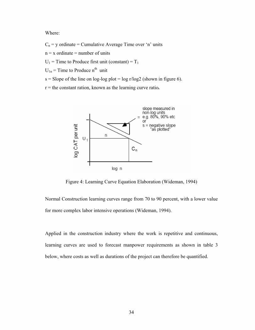
Where:

Cn = y ordinate = Cumulative Average Time over ‘n’ units

n = x ordinate = number of units

U1 = Time to Produce first unit (constant) = T1

U1n = Time to Produce nth unit

s = Slope of the line on log-log plot = log r/log2 (shown in figure 6).

r = the constant ration, known as the learning curve ratio.

Figure 4: Learning Curve Equation Elaboration (Wideman, 1994)

Normal Construction learning curves range from 70 to 90 percent, with a lower value

for more complex labor intensive operations (Wideman, 1994).

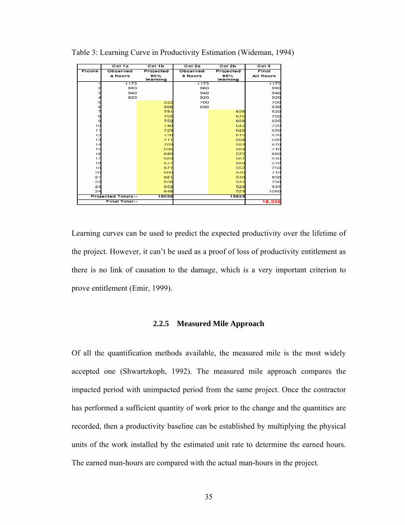
Applied in the construction industry where the work is repetitive and continuous,

learning curves are used to forecast manpower requirements as shown in table 3

below, where costs as well as durations of the project can therefore be quantified.

35

Table 3: Learning Curve in Productivity Estimation (Wideman, 1994)

Learning curves can be used to predict the expected productivity over the lifetime of

the project. However, it can’t be used as a proof of loss of productivity entitlement as

there is no link of causation to the damage, which is a very important criterion to

prove entitlement (Emir, 1999).

2.2.5 Measured Mile Approach

Of all the quantification methods available, the measured mile is the most widely

accepted one (Shwartzkoph, 1992). The measured mile approach compares the

impacted period with unimpacted period from the same project. Once the contractor

has performed a sufficient quantity of work prior to the change and the quantities are

recorded, then a productivity baseline can be established by multiplying the physical

units of the work installed by the estimated unit rate to determine the earned hours.

The earned man-hours are compared with the actual man-hours in the project.

36

When applying the measured mile approach, it is important to separate the variables

that can affect the productivity but are not connected to the change order. For

example, weather, contractor management, overtime, acceleration, delay, crowding,

and the nature of the work completed (Shwartzkoph, 1995).

The impacted period has to be identified and must be compared with an unimpacted

period. The impacted and the unimpacted period must have the same resources. Only

the working condition will differ, and only due to changes because of the owner. The

difference in productivity is the inefficiency due to changes.

2.2.5.1 Sources of Extracting Data to Use Measured Mile

1. Monthly productivity from progress payment request: If a certain job

continued several months then the work quantities in the progress payment

requests to the owner may be used to determine average monthly productivity.

2. Productivity reconstructed from other job records: If the daily records have

enough information to determine the productivity rate yet there is a variability

of the productivity in performing various tasks then such variation can be

accounted for by converting the task in question with an equivalent standard

item and adjusts its productivity. This is the case in the piping work, for

instance, on a sewer claim, the estimated productivity ranged from 33 to 75

linear feet per day for different sections depending on the working conditions.

37

Some sections include manholes, lateral connections, utilities, and other work

items. The variation in the estimated production was accounted for by

converting such work item into equivalent linear feet of pipe.

3. Productivity from historical records on other projects: If the data are not

present, the contractor can use data from past projects of the same nature to

identify their measured mile or unimpacted period. Yet the owner might not

be convinced that the data are similar, so with the contractor should be ready

with convincing tools, statistical analysis and documents to win the case.

4. Patterns of Productivity: A correlation between the impact and the cost

overrun might show the damage (Shwartzkoph, 1995).

The basic concept of the measured mile is to determine an unimpacted period and

linearly extrapolates the cumulative unimpacted hours to the end of an impacted

period and the difference between the unimpacted and impacted is the amount of

damage. As shown in figure 5, the first 30 data points are used as the measured mile.

The projection of the measured mile leads to an approximate of 3,745 h at “100%

complete” assuming that these are the cumulative hours that would have been earned

without any owner-caused impacts. The actual hours expended on the project are

4,810 h (Gulezian and Samelian, 2003).

38

Figure 5: Measured Mile Approach (Gulezian and Samelian, 2003)

2.2.5.2 Proof of Causation

A contractor who is trying to recover disruption damages must be able to prove

entitlement and provide a reasonable calculation of damage. As stated by the General

Services Board of Contract Appeals:

“It has always been the law that in order to prove entitlement to an adjustment under

the contract or for its breach, a contractor must establish the fundamental facts of

liability, causation, and damage” (Warwick Construction Inc.).

The court claimant has noted:

“A claimant need not prove his damages with absolute certainty or mathematical

exactitude…It is sufficient if he furnishes the court with reasonable basis for

computation even, even though the result is only approximate…Yet this leniency as

to the actual measurement of computation does not relieve the contractor of his

39

essential burden of establishing the fundamental facts of liability, causation, and

resultant injury” (Wunderlich Contracting Co.).

The contractor may try to use the difference between the impacted and the measured

mile unimpacted productivity rates as a proof of causation. Such a use can be done

with the “total cost” type of argument in which the contractor proves owner liability

and damage incurred due to the owner then infer causation by proving that the

contractor is not responsible for the lost productivity.

2.2.5.3 Measured Mile Process

The categories of production information needed to effectively track production

efficiencies and support the measured mile method include the following:

– Defining the work activity or cost.

– Account for work performed.

– Logging accurate worker-hours used to perform the work and accurate

quantities of work completed for the period.

– Briefly defining any condition or event that prevented optimum

production such as material deliveries, insufficient design information,

field directives, or changes to the original work scope (Presnell, 2003).

40

2.2.5.4 Measured Mile Advantages

1. Relies on data obtained during actual contract performance.

2. Labor productivity levels for both affected and normal periods are derived

from project records as job cost reports, payroll records, daily logs, and

inspection reports.

3. Avoids the shortcomings of industry studies and estimating guidelines

(Loulakis, Michael C., 1999).

2.2.5.5 Measured Mile Limitations

1. The required data for a detailed productivity analysis might not be

available. Even when the information is contained in the project records it,

can be difficult and time consuming to obtain the data in the format

necessary to perform the calculations. As a result, it can be expensive.

2. It assumes the presence of an unimpacted period at the beginning of the

project (Eden, 2003).

3. The choice of the time at which the base measured mile is very subjective

and can differ from one person to another. Reference to figure 5 above,

the base line can be the first 17 points, or the next 13 points (day 18-30)

41

and that would differ in an amount of damage of 1,420 h and 895 h

respectively according to the choice of the baseline period.

4. Does not provide any causal logic to explain why the impact of changes

would lead to additional work.

5. Can’t separate the effect of changes on the productivity. It assumes that all

the loss in inefficiency is due to the owner. In some projects, contractors

might have some drawbacks in their schedule like underestimating, or

mismanagement.

2.2.6 Baseline Productivity

Regardless of the method discussed above, used to calculate the labor productivity

inefficiency, baseline productivity has to be developed. The measured mile is a

preferred approach, but the baseline for demonstration what the contractor could have

done without the change must be unimpeachable (Loulakis, 2003). The following

studies have been carried out to determine a baseline productivity that the contractor

can compare against in order to determine how the owner changes affect the labor

productivity.

42

2.2.6.1 Thomas Approach

In 2000, Thomas performed a study on how to determine the baseline period. The

baseline period as defined by the authors is “a period of time that represents the best

performance by the contractor”. To define the baseline, it is not a condition to have

continuous, unimpacted time period. The inefficiency due to the owner and the

contractor may be present throughout the project. If the unimpacted period is

continuous then the baseline period and the measured mile are similar. According to

the author, a baseline period can be established without a measured mile analysis. The

difference between the measured mile and the base line is summarized in the table 4

below:

Table 4: Differences between the Measured Mile and Baseline Period (Thomas, 2000)

MEASURED MILE

THOMAS BASELINE

PRODUCTIVITY

The negative impacts should be limited to

those caused solely by the contractor

The baseline period need not be free

of owner impacts

The measured mile time frame should be

several or more consecutive reporting

periods

The baseline time frame need not be

consecutive reporting periods

The focus is on finding periods of time

where there are no owner-caused impacts

The focus is on finding the best

performance the contractor could

achieve

43

Calculations for both approaches depend upon the actual contract performance as

stated in the cost and payroll records. Also both approaches avoid the short coming of

the industry manuals as they rely on data from the same project.

Thomas started by defining the steps to calculate the baseline productivity as follows:

1. Determine the number of reporting periods that comprises 10% of the total

reporting periods.

2. Round this number to the next highest odd number; this number shouldn’t be

less than 5. This number, n, defines the size of (number of reporting period)

the baseline subset.

3. The contents of the baseline subset are the n reporting periods that have the

highest unit production.

4. For these periods, record the unit productivity.

5. The baseline productivity is the median of the unit productivity values in the

baseline subset.

After defining the baseline productivity a data base consisting of 23 masonry projects

was used to present the basis of baseline productivity measurement. For each project

the data were collected using standardized data collection procedures. The data were

processed and converted to a standard item of working using conversion factor.

Various hypotheses were developed from the data base and tested and they are as

follows:

44

• Hypothesis 1—Projects that have good labor performance based on the

cumulative productivity also exhibit minimal variability in daily productivity

values. Poorly performing projects have high variability. Good and poorly

performing projects can be differentiated by the variability in unit productivity

values.

This hypothesis is consistent with the statistical methods used in total quality

management where variation is a measure of quality and consistency. The

hypothesis is evaluated numerically through the use of the disruption index

(DI), where DI measure the variability within single project

daysworkofnumberTotaldaysworkdisruptedofNumberDI

= ………………………......................Eq. 2

• Hypothesis 2—the baseline productivity is a function of the complexity of the

design or WC (work content). As the WC increases (more complexity), the

baseline productivity also increases (worsens). As shown in the table 5 below,

a WC from 1-5 with 5 being the most complex.

45

Table 5: Proposed Work Content for Masonry Database (Thomas, 1999)

WC Scale Description

1 Long straight walls, many greater than 8 m (25 ft) in length; considerable scope of work for each layout; few openings

2 Facades with ordinary window and door openings; openings tend to be at regular intervals, thus minimizing need for different layouts

3 Facades with numerous window or door openings; numerous short, straight walls less than 8 m (25 ft); some ornamental work may be necessary

4 Interfacing with structural steel frame, numerous cutting of masonry units; some poor design details, walls consisting of multiple size units; extensive ornamental work, some corners not 907

5 Numerous corners and walls not at 907; many walls consisting of multiple size units; minimal consistent scope of work

To mathematically test this hypothesis, a linear regression model was developed

Baseline productivity (wh/ft) = 0.045 + 0.016 WC…………………………………Eq. 3

According to Thomas, 2000, the baseline period can be at different periods of time as

follows:

• The baseline is the initial part of the work followed by the impacted

work: Cumulative productivity data can be used if the baseline is at the

beginning of the project. The analysis is similar to a modified total

cost method except that the actual performance is used instead of the

estimated or budgeted productivity.

• The baseline is in the middle portion of the work with impacted work

46

before and after. When the baseline is in the middle, unit productivity

data has to be used.

• Disruption occurs at the end of the work followed by the baseline. If

the baseline occurs at the end it might be affected by the ripple effect.

• The baseline period is sporadic and occurs one day, week, or month at

a time. The author suggested the use of multiple regression to quantify

the loss of each cause.

In the first three cases, the measured mile can be applied, yet the baseline can be

applied in the fourth as it is based on the contractor’s best performance.

2.2.6.2 Control Charts

Another study has been conducted by Ronald Gulezian and Frederic Samelian in

2003 to statistically define the baseline productivity. According to the authors, there

are two types of variations; natural and assignable variations. Natural variations are

those due to common causes of variation. Such variations must be accepted as part of

the performance. For instance, the crew will not perform the same productivity for the

same task from one period to another, even if there are no external conditions.

Assignable causes are those that are not subject to chance and are subject to the

control of the contractor, for instance, scheduling and resource allocation.

47

A control chart is a graphic tool to monitor, asses, and control the quality of a

manufacturing process. Figure 6 illustrates the basic concept of a control chart:

Figure 6: Basic Control Chart Structure (Gulezian and Samelian, 2003)

The metric is the individual productivity value at a particular unit of time.

The Center line is the Arithmetic mean= ∑Productivity values/number of values.

The control limits, Upper Center Line (UCL), and the Lower Center Line (LCL) are

calculated as follows:

UCL/LCL= Center line +/- (3*standard deviation)……………….…………….Eq. 4

Values falling within the center limits are categorized to normal variations, and those

falling outside either control limits are categorized to assignable causes.

48

To determine the baseline under normal operating condition, a control chart is

developed.

Unusual points will fall outside of the set of the control limits will be removed and a

new CL and control limits will be applied till a final iteration where no point lies

outside the control limits and the mean will be the baseline productivity. Further

recommendation is to disaggregate the data so as to account for other factors such as

worker type, types of skill, and other conditions. The following is the approach

recommended by the authors:

1. Use daily labor productivity as a basis for the analysis rather than cumulative

ones to account for the variability in the productivity both in the unimpacted

and impacted.

2. Apply control charts to the productivity values so as to eliminate unusual

values to come up with a productivity value that represents the contractor

normal one.

3. Calculate the baseline productivity as the mean productivity of the

contractor’s normal operating condition.

49

2.2.7 Statistical Approaches

2.2.7.1 Leonard Study

Leonard,1987 performed a study that focused on 90 different case studies from 57

different projects to develop a model for predicting the productivity impacts of

change orders on the base contract work. He examined the relationship between

change orders and productivity. Leonard considered studying three variables and

checked their effect on the productivity and they are: (1) the frequency of change

orders, which was measured as the number of change orders divided by the number of

months of the contract; (2) the average size of change orders, which was measured as

the change order hours divided by the number of change orders; and (3) the

percentage of change order hours, which was measured as the number of change

order hours divided by the actual contract hours, expressed as a percent.

Leonard study showed that the number of change orders issued was not a precise

reflection of the productivity loss, as the correlation coefficient is low. The

correlation coefficient was low as well when comparing the average size of change

order and productivity loss. However a high correlation was found between the % of

change order hours to the total actual hours and the loss of productivity.

He performed a statistical study on the actual change order hours as compared to the

actual base contract hours and showed that there is no correlation between the change

order hours and loss of productivity when the change order hours are less than 10% of

50

the base contract hours.

Leonard study produced six curves to predict inefficiency. His study was classified

into two sections the first one is electrical/mechanical contracts as shown in figure 7

below, and the second is civil/architectural contracts. He looked at the productivity in

both classes as follows:

- Type (1): lost productivity when no other productivity impacting

factor is present (when the only major impact on productivity is

change order).

- Type (2): lost productivity when one other impacting factor is present

- Type (3): lost productivity when two other impacting factors are

present.

Figure 7: Results of Leonard Study (1987)

51

The following equations were used to calculate the inefficiency:

hoursorderchangeactualTotalhoursmanactualTotalhoursbaseActual −−= Eq. 5

hourscontractbaseactualhoursorderchangeActualorderChange / % = …..Eq. 6

The percentage of inefficiency is multiplied by the actual base contract hours to

determine the inefficient man-hours.

The main advantage of his study is that it does not rely on the contractor’s original

estimate. It is based entirely on the actual labor hours. However, his study is based on

a biased sample where the data used were collected from projects that reached the

dispute stage. He did not compare impacted and unimpacted projects. In addition, the

study combined the data for electrical and mechanical trades, where there might be a

chance that the loss of efficiency between the two trades may be different. The study

considered the amount of change as the only factor that caused loss of efficiency. He

did not consider other factors such as timing of change and/or project percent

complete (Hanna, 1999b).

2.2.7.2 Construction Industry Institute Study

The construction Industry Institute CII carried out a study by Ibbs and Allen, 1995.

They studied 89 projects from CII member companies and they had three hypotheses

to be tested:

• Changes at the later stage of the project are carried out less efficiently than

52

those early ones.

• The greater the change, the greater the negative effect on the productivity.

• The hidden or unanticipated cost of change increase with more project change.

According to Hanna, 1999a, such study revealed several limitations and they are

follows:

• In their study to relate independent variables affecting productivity to the

changes, low coefficient of determination, R2, values were recorded.

• In the study, it was assumed that the ratio between the installed material cost

and the total cost is an indication of efficiency for changes that occur late in

the project are carried out less efficiently. Such an assumption can lead to

difficulties when there is a change in scope, or when changes do not affect the

material consumption.

• The study couldn’t prove the fact that changes that occur late in the project are

implemented in a less efficient way than those occur at earlier stages in the

project.

2.2.7.3 Thomas Approach

Thomas (1995b) carried out a study to quantify the impact of changes on labor

productivity and the relationship between changes and various type of disruption.

Electrical and piping crafts were studied. The work performed by such crafts was

narrowed to the crews related to the production work as installing conduit and pulling

53

cable. The projects selected are ones that were not anticipated to experience lots of

changes. In addition, the early phase and the start up phase were not considered in

such study. The author stated that although many changes may be experienced at this

phase, statistical analysis using this data is hard to be performed plus the work at this

stage is not conducive to good productivity.

The data were collected with the aid of seven forms filled everyday and one filled for

each project the forms are:

• Form 1: Manpower/labor pool crew size, crew composition (skilled or

unskilled), and absenteeism.

• Form 2: Quantity measurement.

• Form 3: Design features and work content.

• Form 4: Environmental site conditions; temperature humidity.

• Form 5: Management practices; delays, material, equipment and information

availability, congestion and work sequence.

• Form 6: Construction method work day, overtime schedule and working

foreman.

• Form 7: Project organization; type of the project workforce, other site-support

personnel and number of foreman.

• Form 8: Project features: type of the project, approximate cost, approximate

planned duration.

54

Following the form completion, a data processing phase was carried out. The purpose

of this phase is to calculate the daily productivity and screen the data for any unusual

trend so that the productivity is related to a baseline when there are no changes or

disruption to the work.

Through conversion factors the productivity of crews doing a variety of work can

have their output expressed as an equivalent item of a single standard item. In this

way, the productivity of all crews can be calculated for the same standard item during

each period regardless of the work done. Similarly, the data from different projects

can be combined after calculating the conversion factor against the standard item

(Thomas, 1997).

itemdardstheofrateUnitquestioninitemtheofrateUnitfactorConversion

tan = …………………………Eq. 7

Equivalent quantities are the number of units of the standard item that will yield the

same number of earned hours as was actually earned by installing nonstandard item.

Equivalent quantity = ∑ (Conversion factor X Actual qty.) for the total item installed.

Baseline productivity is determined for each data set by choosing the work hours and

quantities installed on days when no changes or rework, disruption or bad weather

were reported. The deviation of the actual productivity from the baseline is measured

by the performance ratio (PR) where PR is:

55

typroductiviBaselinetyproductiviActualPR

= ……………………………………………………Eq. 8

PR more than one indicates that more hours were spent than the baseline. In other

words, the productivity is worse than the baseline.

Multiple regression was used in the quantification of the effect of changes on labor

productivity. The first phase of the study is hypothesis testing, where the hypothesis

examined is:

Ho= an independent variable produces statistically no differences in the dependant

variable.

H1= an independent variable produces statistically significant differences in the

dependant variable.

For the significance of individual variables, an ANOVA test was done for each factor

at a time with the PR as the dependant variable.

Multiple regression equation was developed in which the performance ratio is the

dependant variable and the disruptions are the independent variable; the quantitative

effect of the disruption is shown in table 6.

56

Table 6: Quantitative Effect of Disruption (Thomas, 1995b)

Disruption Type Efficiency

Material Availability 0.74

Tool Availability 1.06

Equipment Availability 1.05

Information Availability 0.53

Sequencing 0.71

The author concluded that, the time of the change is a crucial element. The change its

self does not cause loss of efficiency, yet it’s how the change affects other variables,

and these are the ones that reduce efficiency (Thomas, 1995b).

The main disadvantage of this model in most construction projects several problems

might occur at the same time so it is important to develop a model that tests how

significant the results will be when some/all the potential variables are present.

2.2.7.4 % Delta Approach (Hanna, 1999a, b)

Hanna conducted several studies on Electrical/Mechanical projects. The loss of

efficiency is determined by factor “delta”, which is the difference between the base

project labor hours (actual total project hours less the estimate of change order hours)

and the original estimate of labor hours at the contract award.

As shown in figure 8, positive delta indicates an actual productivity less than planned

57

and that might be due to several reasons such as contractor’s low estimate,

contractor’s inefficiency, and the impact of other factors such as weather, work

interruptions, and others.

hourslaboractualTotal

hoursorderchangehoursbudgetedhourslaboractualTotalDelta 100*) ( % +−=

Eq. 9

Figure 8: Graphical Illustration of Delta (Hanna, 1999b)

According to the authors, at least the first and one of the other following criteria

would decide whether the project is impacted or unimpacted.

1. Planned versus actual loading curve—Coffman (1997) indicated that a project

is considered impacted by change orders when the actual and planned

cumulative work hours vary substantially. The actual loading curve can take

58

two forms. One form is a loading curve without time extension, and the other

is a loading curve with time extension as shown in figure 9.

Figure 9: Planned and Actual Loading Curves (Hanna, 1999b)

2. Time extension—Projects that are impacted by changes are characterized by

an extension beyond the originally planned duration.

3. Timing of change orders—Changes issued in the latter part of projects tend to

have a more negative impact than changes issued when the project is <50%

complete (Ibbs and Allen 1995).

4. Lead-time—Lead-time is defined as the amount of time available between

making a change and the actual completion the work. If the lead-time is small,

59

loss of efficiency tends to be much higher than when the lead-time is

adequate.

5. Ripple effect—There is a strong correlation between projects impacted by

changes and schedule compression, stacking of trades, and over manning.

This indicates that change orders can create another set of productivity-related

problems such as schedule compression. Such a trend supports the need for

macro analysis to quantify the impact of change orders on labor efficiency.

After the projects are classified according to the above criteria as impacted or

unimpacted, the contractors participating in the research fill another questionnaire, to

define the sources of impact on labor efficiency and their effect. For each source of

impact, contractors give a score from 0-5 that indicates the degree of impact.

The data analysis was divided into two parts; the first part is hypothesis testing to

determine whether the projects are impacted or unimpacted. The second step is a

regression analysis to develop a model for the impact of changes on the labor

efficiency.

In hypothesis testing step, the data was grouped into two discrete categories

• Projects that experience any of the criterion mentioned above (at least the

first one and one more of the other)

• Projects that do not experience any type of productivity losses.

60

The amount of change was calculated in two ways, to determine if there is any

relation ship between the amount of change and the amount of impact on labor

efficiency.

a. The total amount of change order hours that occur in a project.

b. Amount of change measured as a percent of the project size. This is

achieved by taking the estimated change order hours as a percent of

the estimated base hours and the total actual hours.

The results showed that the percent of the change of labor hours over the estimated

base hours is very significant. The relationship of the amount of change, measured as

a percent of the change order hours/ estimated base hours and delta as a percent of the

total labor hours for both impacted and unimpacted projects were plotted, and a

significant relationship is shown between the amount of change and the amount of

impact on labor productivity.

The author was interested in exploring the timing effect of the change order and its

effect on the labor productivity. The cost of change increases as the project moves

toward completion. The impact of the changes later in the project tend to have more

impact on the labor productivity due to the limited time to perform the changed work,

large amount of material to be delivered and installed and crew interruption (Chick,

1999). In an attempt to test this concept, a questionnaire was developed where the

respondents were asked when during the project, the change orders took place. The

61

variable weighted timing (WTIMING) was used to measure when the change orders

occurred. The project was divided into six equal segments. Each segment was given

an indicator variable beginning with 1 for the segment before construction and ending

with 6 for the final segment from 80 to 100% as shown in table 7. The fraction of

change that occurred during that portion of the project was then multiplied by the

specific indicator variable. The sum of these values for a given project is defined as

WTIMING. After the WTIMING value was calculated, a comparison was held

between the outcomes for both the impacted and unimpacted projects. The p-value for

the statistical test is 0.7478.This shows that there is no statistically significant

difference in the value of WTIMING between impacted and unimpacted projects. The

WTIMING for the projects versus the dependent variable, delta as a percent of total

labor hours, was then plotted. The results do, however, appear to show a relationship

in WTIMING and the amount to which labor efficiency is impacted.

Table 7: Weighted Timing Example (Hanna, 1999b) Fraction of Change Orders Occurring in Portion of Project X Indicator Value

(Segment of Project)

Project

1(<0%) 2(0-20%) 3(20-40%) 4(40-60%) 5(60-80%) 6(80-100%)

WTIMING

1802 0.00 0.00 0.25 0.00 0.50 0.25 4.75

1605 0.00 0.10 0.35 0.00 0.35 0.20 4.2

114 0.00 0.20 0.40 0.00 0.40 0.00 3.6

The second step after the hypothesis testing is the model building. Stepwise

regression is used to allow adding one variable at a time to the model and removing

from it as well at any time. SAS software was used to analyze the data. A total of 61

62

projects were used for model formulation and 10 extra for the model validation. Delta

as a percent of the total labor hours was selected to be the dependent variable.

For the model validation ten projects were used, which are not used in the model

formulation. A confidence interval of 90% was chosen in the study. All except one

project fall within the limits.

In another study by Hanna, 2002, he aimed to quantitatively define whether an

electrical or mechanical project is impacted by change orders. He developed a

questionnaire that included three sections. The first section consisted of general

background questions about the contractor, and the other two were for projects

selected by the contractor, of which one section was for an ‘‘on budget’’ project and

the other was for an ‘‘over budget’’ project caused by change orders. Also, actual and

estimated manpower loading curves or weekly labor hours were requested for each

project along with a change order log.

The authors define the project as impacted or unimpacted based on a question on the

survey of whether the project is over budget or on budget based on the budget labor

hours defined as the total estimated hours that the contractors used to allocate the

labor resources. Impacted project less than 5% delta are considered to be unimpacted.

The study involves a hypothesis testing and a logistic regression analysis

The % delta approach has several limitations. In a Discussion performed by Ossman,

2002 on Hanna’s model, he mentioned the following concerning Hanna’s approach:

63

Reference to the equation to determine % delta which is,

hourslaboractualTotalhoursorderchangehoursbudgetedhourslaboractualTotalDelta 100*) ( % +−

=

Eq. 9

Since impacted hours = Total actual labor hours-budgeted hours-change order hours,

which is the same calculation used in the total cost method that is mainly rejected in

the courts. As stated in Amelco V. City of Thousand Oaks (California Supreme Court

No. S091069, filed 2/4/02) the following four actions have to be considered before

using the total cost method, which should be the same precautions before using

%delta indicator:

- “the impracticality of proving actual losses directly”

- “the plaintiff’s bid was reasonable

In addition, Hanna assumes that the budgeted hours are reasonable calculation. Since

the survey was filled by contractors where they were asked to fill the questionnaire

for projects they have cost overruns, the contractor might unknowingly regard the

project losses as to be due to change orders rather than other causes that can be in his

control.

- “its actual losses were reasonable, and

- it was not responsible for the added cost”

According to Ossman, %delta is not an appropriate indicator of disruption or impact

as if the contractor experiences a labor hour overrun because of changes for which the

owner is held responsible, he has to be compensated for it. Applying the % delta

equation in this case, %delta =0. Thus this case which both parties equivocally agreed

64

that change orders affect the work is not represented by this equation.

Ossman suggested that a study of the projects where are all parties involved,

including owner, contractor and subcontractor, are interviewed to study their

individual assessment of the use of labor hours originally planned for the project

versus the ones actually used. This would provide a broader view of the problem

allowing a more reliable quantitative measure of impact.

In another discussion by

The use of questionnaire led to a biased study especially that it is filled by contractors

who are encountered productivity losses because of the owner change orders. The

way the questionnaire was developed directed the contractors to consider the projects

impacted if it is over budget. Over budget is not an indication of productivity loss as

the contractor might unconsciously ignore his management on site or underestimation

of bid prices to get the job in the first place. Some contractors underestimate their

bids to get the job and view the change orders as a profit center where they will get

the profit from. In addition, the model builder did not rely on the actual plans, specs,

daily productivity and changes of the project, just relied on the reply of the contractor

filling survey.

In another discussion by Farbaric, 2002 on the study performed by Hanna on the

impact of change orders on labor efficiency of electrical projects, 1999b, he discussed

that the authors performed an error in stating that “a strong relationship between each

65

of two independent variables and a dependent variable implies a strong relationship

between the two independent variables. This is an error both in statistical data

interpretation and in basic logic “. (‘‘All cows have four legs. All horses have four

legs. All cows are horses”) (Farbaric, 2002).

In addition, Stepwise regression, which was used in the model building stage, has

several limitations especially in this application, and they are as follows:

- Automated model building does not facilitate subjective modeler input.

The choice of the factors is performed by the researchers and there is

always a possibility of bias or prejudiced choice. Also, according to the

author, the statistical significance tests (t-tests and p-values) are used for

the selection of the factors. However, such approaches have limited ability

to produce an unbiased factor selection in the case where there are

complicated interactions between factors with different characteristics

(numerical, categorical, and split).

- The degree of correlation between the predictor variables affected the

frequency with which predictor variables found their way into the final

model.

- Stepwise methods will not necessarily produce the best model if there are

redundant predictors (common problem).

66

- The size of the sample was of little practical importance in determining the

number of variables contained in the final model.

- Models identified by stepwise methods often fail when applied to new

datasets so we can’t generalize it to be used for other projects.

- The lack of the ability to show the relationship between the factors.

- It is based on methods (e.g. F tests for nested models) that were intended

to be used to test pre-specified hypotheses (Dreksen, 1992).

2.2.7.5 Decision Tree (Lee, 2004)

In 2004 Lee et. al adopted the use of decision tree to quantify the effect of change

orders in increasing the productivity loss. In this study, two types of decision trees are

used:

1. Classification tree: In this study, classification rule with unbiased interaction

selection and estimation (CRUISE) is used to develop a model that can

classify project impacted by change orders. In this study 142 case studies were

used in which 69 projects were impacted and 73 unimpacted. The projects are

classified as impacted or unimpacted by change orders according to a survey

filled by contractors participating in the research. Each case study is

composed of around 70 independent variables and one dependant variable

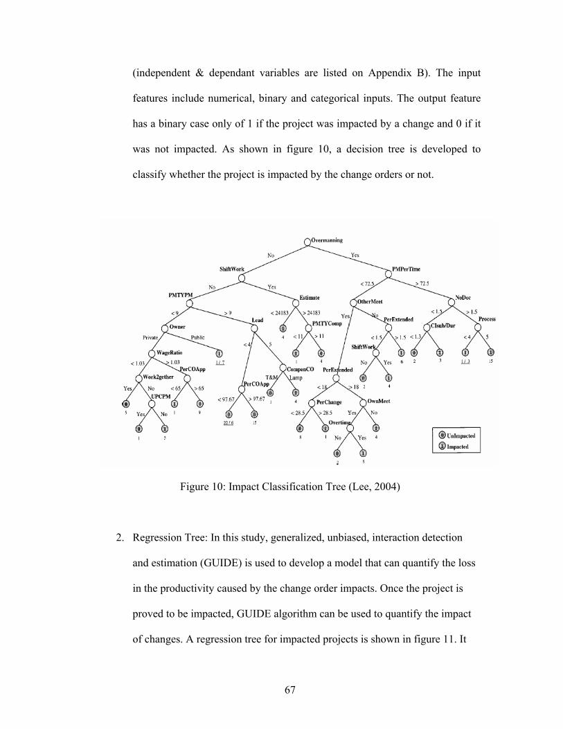
67

(independent & dependant variables are listed on Appendix B). The input

features include numerical, binary and categorical inputs. The output feature

has a binary case only of 1 if the project was impacted by a change and 0 if it

was not impacted. As shown in figure 10, a decision tree is developed to

classify whether the project is impacted by the change orders or not.

Figure 10: Impact Classification Tree (Lee, 2004)

2. Regression Tree: In this study, generalized, unbiased, interaction detection

and estimation (GUIDE) is used to develop a model that can quantify the loss

in the productivity caused by the change order impacts. Once the project is

proved to be impacted, GUIDE algorithm can be used to quantify the impact

of changes. A regression tree for impacted projects is shown in figure 11. It

68

was developed using the stepwise regression.

Figure 11: Quantification Tree model (Lee, 2004)

A model is developed for each node. Reference to the above figure, having good AE

coordination with more than 15%of change orders caused by design problems and a

delayed project greater than 33% of the original duration lead the user to terminal

node 5. The regression equation at node 5 is as follows:

% delta = 0.401-0.162XEA/PA-0.0315XProcess+0.003XPERdESIGN……….Eq. 10

The average error in %delta is 20.7% for the tree model while it is 53% for the

regression model prepared by Hanna 1999a. The tree model represents the actual loss

through the entire range whereas the regression model gives poor representation in

the area under 20 % ( %delta) of the actual loss range.

69

Though decision trees are easy to apply however, decision tree algorithms are

unstable. Slight variations in the training data, which the data set used to build the

model, can result it different attribute selections at each choice point within the tree.

The effect can be significant since attribute choices affect all descendent sub trees.

Thus we can’t generalize this decision tree to the entire industry and the courts can’t

rely upon it as a tool to prove entitlement. In addition, in case where there are

qualitative variables, there is a necessity of factoring in the qualitative factors which

will be discussed in details in Chapter 3, and if there are many qualitative variables,

which is the case in this study the tree can be long and complicated.

2.2.8 Neural Network

Several researches have used the AI tools like the neural network to quantify the

impact of change orders on labor productivity. One of the most recent studies is a

research done by Moselhi et al 2005. The main goal of this study was to develop a

neural network model to predict the effect of change orders on the labor productivity.

The model was done in three main stages, first identifying change order factors that

affect labor productivity. Second modeling the timing impact, and finally developing

a neural network model

Based on a thorough study of field labor productivity the following factors affect the

impact of change order on labor productivity:

a. Intensity: This factor can be represented as number of change orders, their

frequency; and/or the ratio of change orders hours to contract hours. The

70

ratio of change orders hours to planned or actual contract hours is mostly

used to represent this factor. (Leonard, 1987; Moselhi et al. 1991; Ibbs

1997; Vandenberg 1997; Hanna et al. 1999a, b).

b. Timing in relation to project duration: Coffman, 1997 pointed out the

significance of the timing factor stating: “When evaluating change orders,

regardless of their cause, the most significant factor is when the change

occurs.” The timing factor has been pinpointed by Hanna et al. 1999b

assuming that the timing impact increases from project inception to

completion in a linear manner. This assumes higher labor productivity

losses to occur toward the end of project duration, and therefore it does not

consider the ripple effect of change orders on the remaining unchanged

work.

c. Work type: The impact of the changes on productivity differs according to

the type of work i.e., civil, architectural, electrical, or mechanical

(Leonard, 1988). This is mainly due to the differences in the level of skill

required to perform the work and its degree of complexity; the

interdependency which varies from one type of work to another and

among work types (Coffman 1997; Leonard 1987).

d. Type of impact: Change order themselves does not cause a negative

impact on the productivity, yet it’s the other variables that are affected due

71

to this change like overtime, over manning, congestion and other related

factors.

e. Project phase: This factor differentiates between changes introduced

during the design phase and the construction phase.

f. On-site management: This factor relates to the Project Manager’s years of

experience (Hanna et al. 1999b).

As introduced by Hanna 1999a, he had a hypothesis that assumes that the impact of

the changes increase from project start to completion in a linear trend. Such

hypothesis was not supported by the results of other researchers. For instance,

Bruggink, 1997 and Coffman, 1997 stated that the highest impact of change orders

takes place in the third quarter of the project duration. Also, Ibbs and Allen, 1995 did

not find that changes which occur late in a project are carried out in a less efficient

way than changes that occur early. In this study, 33 cases were analyzed by plotting

the direct manpower loading curve over the duration of the project.

To compare this study with Hanna study, 1999a, the project was divided into 5

portions. Man hour loading ratio, which is the ratio of the hours in time to the entire

project, was calculated for each segment.

Bent and Thuman, 1988 and the AACE Education Board, 1989 suggested a typical

trapezoidal shape to model the direct manpower loading in construction. The National

72

Electrical Contractors Organization NECA 1983 developed an industry-average type

curve, to represent the manpower distribution along the electrical project. In this

study the first approach was used for general construction projects, whereas the

NECA was used for the electrical projects.

The timing impact of change order (TP) for each segment was calculated using the

following equation:

)()()(

tPHtHCOtTP = ………………………………………………………………Eq. 11

TP= timing impact of change order in period t HCO= actual change order hours in period t PH= planned hours in period t t=time when the change order occur, where t= 1 to 5.

The model was developed using NeuroShell2 which operates in the MS Windows

environment and offers a number of ready-to-use neural network models.

A prototype software system was created to provide a tool for quantifying the

negative impact of change orders on labor productivity. The software provides a user-

friendly interface and incorporates the newly developed neural network model; and

the previously developed models for general construction which includes, Moselhi,

1991a; Ibbs 1997, mechanical construction, Hanna 1999a and electrical construction

Hanna et al., 1999b.

A comparison of the results revealed that the proposed model was a better tool than

the available models in estimating the impact of change orders on productivity losses.

73

The average estimating error of the proposed model for the analyzed eight cases was

17.8%, which is significantly lower than those 30.5% and 40.5%associated with the

general regression model of Moselhi 1991 and the electrical regression model of

Hanna 1999b. The average absolute estimating error of the proposed model, the

general regression model, and the electrical regression model was also calculated to

be 19.4%, 25.3%, and 30%. This shows that taking into account the timing impact in

the developed neural network model was vital in enhancing the accuracy and

reliability of estimating the impact of change orders on productivity losses.

Neural network however has several disadvantages especially in these applications.

Neural Network models are in a sense the ultimate 'black boxes'. Initially seeding it

with a random numbers, the user has no other role than to feed it input and watch it

train and await the output. In fact, "you almost do not know what you're doing". The

final product of this activity is a trained network that provides no equations or

coefficients defining a relationship (as in regression) beyond its own internal

mathematics (Donald, 2002).

Thus concerning the application of neural networks in the quantifying the change

orders, it appears that it is not an applicable tool as the model builder need to have

input on the choice of the predictors per say and not just rely of the computer output.

74

2.3 Summary

As shown in the above section, the previous researches in this area suffer from

drawbacks that limit their use and made the entitlement to loss pf productivity

damages hard to prove. The main drawbacks are the use of questionnaires reflecting

only the perspective of one part over the other; in this case it is the contractor, the use

of the bid-hours, which is not a reliable value, to compare with the actual damages as

a proof of entitlement, the statistical approaches used to build the productivity loss

models, and the missing information in the industry standards. All of these drawbacks

might discourage owners and courts to provide entitlement to the contractor in case of

productivity loss due to change orders.

75

CHAPTER 3: METHODOLOGY

3.1 Background

The objectives of this study are: 1) To analyze and develop a model to quantify the

percentage increase of the contract value due to change orders. 2) To quantify the loss

of labor productivity for the sanitary sewer/storm water piping work due to change

orders. The study is applied on heavy construction projects that encountered change

orders and where the change orders impacted the contractor’s performance in the

changed area. In this way the researchers will be able to determine the main causes

that contribute to the increase in the contract value and the ones that contribute to the

contractor’s labor productivity losses due to change orders.

The study will be divided into two parts. The first part will concentrate on the percent

increase in the contract price due to change orders and the second part will focus on

the labor productivity loss.

3.2 Data Collection

The most important step is to define the projects criteria under study. This is

achieved through running multiple interviews with several claims consultants that

handled construction claims for both the owner and the contractor. In addition

interviews were conducted with a public owner to understand the major problems

76

they believe might be the cause of the increase in the contract price due to change

orders and productivity loss.

The main projects criteria are:

Projects Type: Heavy Construction (road projects).

Owner Type: Public Owners.

Delivery Method: Design-Bid-Build.

Data Source: Daily Reports, Plans, Contract, log of changes & Claims

documents.

Projects 100% completed.

Projects where claims were encountered and resolved.

Projects studied are ones where the original contract amount ranges between $10M-

$25M projects. The second most important step is to define what are the data required

to build the model. The researchers will rely on the actual owner daily reports and

change orders that are mainly used by the contractor when they claim entitlement to

damage. The researchers did not use questionnaires to avoid any potential bias.

Figure 12 summarizes the data collection steps performed to collect the data.

77

Figure 12: Data Collection Procedures

3.3 Data Preparation

After collecting the data from the projects it is important to prepare the data to start

the model building step.

Explain Research Objective

Contact District Construction Office & Hold Meeting

Collect Data from Each District

Start Data Preparation for Model Building

Study the Projects Selected: Problem areas, reason for changes/claims

Identify Projects Criteria • Road Projects • Design-Bid-Build • 100% completed • Claims are resolved

Identify Documents Required for each Project Selected

• Contract • Daily Reports • Change Orders Issued • Drawings • Claim Documents

78

3.3.1 Change Order Study

Change orders are very common in most construction projects. Changes occur not

only because of errors and omissions, but for other reasons like changes in the scope

of work, or changes because of unforeseen conditions encountered on the site; a

problem which is very common in most roadway projects.

The first step in this research is to study the change orders. The main aim of this study

is to understand how various attributes for the change order affect the value of the

change.

The change order value is measured as the value of the change order over the total

amount of accepted change order value. It will be referred to in this study as the

dependant variable.

3.3.1.1 Dependant Variable (Response):

The main objective of this study is to quantify the percent increase in the contract

price due to change orders to be used by the owner for forward or retrospective

pricing of the change. The percent increase is measured as the cumulative cost of the

change order over the original cost of the project. The owner will be able to use this

model to provide a retrospective or forward pricing of the change orders especially

when facing with exaggerated change order cost proposals from the contractors when

the change order is issued.

79

($) ($) %

projecttheofCostOriginalDatetoOrderChangetheofCostCumulativechangetoduepriceconractinIncrease =

Eq. 12

3.3.1.2 Predictor Variables

As shown in figure 13, eleven predictors are applied to analyze and quantify their

effect on the price increase of the contract due to change orders; they will be referred

to in this study as the independent variables:

80

Figure 13: Predictor Variables for Change Order Study

81

Timing of the Change Order:

The cost of change increases as the project moves toward completion. The impact of

the changes later in the project tend to have more impact on the labor productivity

due to the limited time to perform the changed work, large amount of material to be

delivered, and constructed and crew interruption (Chick, 1999).

There are many types of construction changes and each type can have an effect on

labor productivity. The change itself may not lead to lost productivity, as the change

can be for a constructive reason like reducing a project’s cost or improve its overall

lifecycle value. To a great extent, the type of the change is not as important as the

existence of the change, the effect of the change on the unchanged work, and the time

such change was issued.

Changes occur during the life time of the project for various reasons. Changes occur

not only because of errors and omissions, but for other reasons like changes in the

scope of work, or changes because of unforeseen conditions encountered on the site; a

problem which is very common in most roadway projects. Changes can also be to

overcome the contractors errors either errors in the bidding stages; or errors during

construction.

Changes may occur late for several reasons. One reason is that some discrepancies,

omissions and needed work changes are not discovered until latter stages of the

project. Another reason for late changes is that the project parties may be hopeful that

82

they can agreeably solve disagreements. Eventually all of the issues in conflict may

have to be raised to the attention of a higher organizational or formal level of review,

by which time, the cost and time impacts have increased. Another reason for late

change may be that owners may want to add more features to the project if there are

available funds as the project going to later stages. Unspent contingency moneys may

be a source of such “scope additions” (Ibbs, 2003).

The “Timing of the Change Order” factor is measured in % as:

)( ))( * (

DaysdurationcontractOriginalDaysproceedtoNoticeresolvedorderchangeDate − X100………..……Eq. 13

*Date CO resolved: the earlier of the issuance of the Change Order date or the

clarification date of a request for information (RFI) that led to changed work with a

directive from the owner to construct the change till CO is issued.

Reason for the Change:

There are several reasons for the owner to issue a change order. The magnitude of the

amount of the change differs from one reason to the other. The following are potential

reasons for why an owner may issue a change order for:

A. To provide for major quantity differences, which results in the

contractor's work effort exceeding the original contract amount.

B. To provide for unforeseen work, grade changes, or alterations in the

plans which couldn't reasonably have been contemplated in the

original plans and specifications

83

C. To change the limits of the construction to meet field conditions, for

example extending the project construction limits.

D. To make the projects more functionally operational; for example

asking the contractor to perform extra work on site that was not agreed

upon in the contract just because the contractor is on site and hiring a

subcontractor to do this work might be more expensive and time

consuming.

E. Deterioration or damage to the project after design due to accidents,

weather conditions, and others.

The Party Implementing the Change Order:

A study of the party implementing the change order whether it is the contractor or the

subcontractor is important. If the change order is performed by the subcontractor, the

process might take more time and hence increase the cost of the change as the owner

will request a cost proposal for the change order from the contractor and then the

contractor will pass the request to the subcontractor. This process can be very timely

and costly especially if they did not agree on the cost of the change order.

Work Stoppage: It is not uncommon that the contractor has to stop the work when a change order is

issued. The contractor might need to take labor from one area to the area where

change order will be executed, or when the contractor encountered a conflict and

waiting for the owner to direct him of what to do.

84

This problem is very common when the contractor is lacking the management

experience in handling the change order. According to most of the contracts, the

contractor has to continue the work even when there is a disagreement on the cost

proposal provided by the contractor.

This factor is a binary variable of whether the change led to the work stoppage and

this factor is very much related to the reason of the change.

Change Order Expended as Rework/ Credit (either addition or deletion)/

Idle:

This variable is to check how the way the change order is expended affects the cost of

the change order. Does the change order when it is due to work addition or deletion

cost more, or when it is a rework of an activity already completed, or when it is

issued to compensate for idle labor due to the change.

Credit:

Addition: “An item of work not provided for in the contract as

awarded but found essential to the satisfactory completion of

the contract”.

Deletion: “items contained in the Schedule of Pay Items are

found unnecessary for the proper completion of the work”.

85

Rework:

“Redoing work in the field regardless of initiating cause or

source”.

Idle:

“Labor who stopped their normal planned work due to the

change order issued”.

The Way the Change Order is Compensated:

Usually the contractor provides a cost proposal to the owner for performing the

changed work and if the party with whom he has a contract accepts the price, the

contract is modified in accordance with the terms of contract. When the contractor is

preparing a cost proposal for the changed work, it is important to include all the costs,

overhead and profit. In addition to the actual cost of performing the changed work,

the contractor should include as well the cost effects on other activities under the

contract. For example, performance of the change order may require taking a crew or

a supervisor or both from the planned contract work to work on the change. This will

cause disruption in the planned contract work and increase the cost of the unchanged

work.

In addition, there is additional home office or field engineering, estimating and

purchasing services, which has to be added to the cost of the change.

A separate item of the contractor cost proposal should be for the cost of preparing the

change order quotation and the proposal should state entitlement to that cost, with

86

overhead and profit whether the change is ordered or not. The change order can be

compensated as unit price or time and material or as a lump sum amount negotiated

between the contractor and the owner.

This variable will show to the owner which way of compensating for the change will

lead to an increase of the cost of the change order. The change order can be

compensated as:

Unit Price:

If the bid contract is based on unit prices or lump sum bid supplemented by unit price

quotation, contractor will have to follow those unit prices unless the original

quotation made provisions for higher unit prices for smaller quantities. Prices based

on larger quantities are seldom adequate to cover the cost of change orders. Some

contract documents allow for equitable adjustments for unit prices if substantial

inequity would result from their use for change order pricing.

Different unit prices for deleted items are appropriate when a large deletion will

significantly increase your cost of remaining units.

Time & Material:

In some case the contractor may be authorized to proceed with the change order and

bill the owner for time and material spent to perform the changed work. This may

initially appear to be the most acceptable method of pricing, but it will not prove so if

87

the owner refuses to pay the bill as he might consider the time and material to be

excessive.

In as much as, most owners, architects and general contractors does not have the

awareness of how much extra the change order can cost more than the bid work.

Lump sum:

Change orders may be paid by reimbursing the contractor for direct cost plus a

percentage or fixed amount for overhead and profit. Agreement may be difficult to be

reached on what is the direct cost and what would be paid by the contractor out of his

overhead and fee. So they might reach a negotiated amount that is agreeable to both

parties.

Restricted Access:

Sometimes the owner issues a change order and this change lead to restricted access

by the contractor labor, and hence reduces the labor productivity and increase the cost

of the change. The owner needs to give more attention to this problem when he issues

a change. This factor will be an indication to the owner of the effect of the restricted

access as a result of the change to the cost of the change.

Change Order Work Season:

This is to check the effect of the season of the changed work relative to the planned

work at the time of the bid.

88

Stacking of Trades:

Stacking of trades occurs when worker from different trades work at the same area

(Sullivan, 2002). Workers from different trades might work in the same area as a

result of the change and this cause loss of productivity due to the congested site.

Staking of trades can occur due to different causes; rework, scope change, change

order, project acceleration, complexity of work, poor planning, and delay in

preceding activity.

Approved Change Order Hours:

Most of the consultants interviewed believed that the greater the approved change

orders, the higher is the percent increase of the change order. As approved change

order hours will consist of labor and equipment hours, either operating or idle.

This variable is measured as:

100)

( XprojectthefororderchangeapprovedTotal

orderchangeeachforissuedorderchangeApproved …………….…Eq. 14

Extension:

According to the type of the delay, the change order cost is calculated. For excusable

but non-compensable type of delay, change orders will be issued with days of

extension but no extra cost. When the change order affects a controlling work item

(critical activity) the change order will be issued for extra time and money. This

factor to check if there is any relation with the extension of days granted and the

increase of the contract price due to the change orders.

89

This factor is measured as:

100)

( XdaysinprojecttheofdurationOrginal

orderchangeeachforcontractorthetoentitledextensionofDays …...Eq. 15

3.3.2 Loss of Productivity Study

3.3.2.1 Introduction

The heavy Construction include establishments whose primary activity is the

construction of entire engineering projects (e.g., highways and dams), and specialty

trade contractors, whose primary activity is the production of a specific component

for such projects. Specialty trade contractors in heavy Construction generally are

performing activities that are specific to heavy and civil engineering construction

projects and are not normally performed on buildings. Activities that are common in

most heavy construction projects include, clearing and grubbing, excavation work,

utility work (includes sanitary sewer, storm water drainage and potable water),

paving, and traffic control.

Utility work is a one of the most crucial activities in roadway projects. Failure to

properly drain a pavement can cause many problems. Water on the surface

encourages mosses, algae and other vegetation to colonize the paving; in icy

conditions even shallow puddles can become extremely dangerous ice rinks and over

the longer term, standing water can actually damage the paving itself.

90

Studying the change order of roadway projects, it was discovered that several change

orders are issued because of conflicts encountered in the piping work, or for design

errors and where productivity loss is encountered by the contractor. In most cases, the

contractor passes the full blame of the productivity loss due to change orders to the

owner. There are several factors attributed to the contractor beside the change orders

that can affect the productivity due to changes such as dewatering problems, accident

on site by the contractor’s resources, and material problems.

In the past 3 years, Florida Department of Transportation (FDOT) experienced

increased change orders due to utility adjustment delays, changes to utility Joint

Project agreement, utility work with wrong size, wrong location, or changes to

accommodate required drainage modification.

This study will focus on measuring the loss of the productivity for the piping work.

The productivity measure will be expressed as man-hours per unit length.

The following are the activities that are used to measure the productivity as shown in

figure 14:

A. Trench Excavation:

B. Pipe Bedding:

C. Pipe laying

D. Backfilling & Compaction

91

Figure 14: Piping Activities (A J Mccormack & Son, 2006)

The productivity for the piping work that includes the above activities will be

measured from one structure to another. Man-hours and quantities will be extracted

from the daily report of the owner and the drainage plans. A sample of a drainage

plan from a state project under Florida Department of Transportation (FDOT) is

shown in figure 15 below.

Figure 15: Drainage Plan (FDOT)

92

The day’s footage of cut trench should exceed only by a small amount the pipe

footage to be laid (and partially backfilled) in order to minimize the exposure of the

empty trench to be affected by rain. The day’s production will depend on the slowest

of the excavation and the pipe laying crew. Thus in a deep trench the extra excavation

required may reduce the footage of the pipe laying crew.

Wherever excavations of the trench expose unsuitable materials such as peat, soft

clay, quicksand or other unstable material in the bottom of the trench, unsuitable

foundation to support the pipe, backfill and expected superimposed loads, such

unsuitable materials must be removed to a depth necessary to reach material having

adequate bearing capacity and at a width of trench at least equal to the minimum

trench width as specified.

The pipe laying operation starts by hand trimming till the proper sub grade, then the

pipe is lowered to position. “Pipes should be laid in straight lines to a steady gradient.

A taut string line, sight rails or, more commonly nowadays, a laser line is used to

ensure accuracy in alignment and level. Pipes should be laid on a full bed of granular

material and not propped up on bricks, bits of stone, broken flagstones etc. The pipe

should be consolidated into the bedding or have the bedding packed beneath it until it

is at the correct alignment and level as indicated by the guide line” (FDOT, 2004).

93

3.3.2.2 Dependant Variable

As discussed in Chapter two, numerous studies have been conducted to quantify the

productivity loss due to the change orders. Most of the studies compared the actual

productivity to baseline productivity and they considered the bid hours as the baseline

productivity (Hanna, 199a, b). As previously mentioned, the bid hours are not

considered as a reliable source to compare to in claims as this method of comparison

is similar to the “Total Cost Method” that is rejected in court and similarly most

owners are strict in providing any kind of entitlement for contractors using this

method as a proof of damage.

In this study, the baseline productivity is the average best productivity achieved by

the contractor. This method is similar to the measured mile, and Thomas baseline

approach discussed in Chapter 2 except that the researchers do not only include man-

hours, but also quantities in the productivity equation. Previous studies showed that

there is a correlation between the quantities installed and the productivity rates and

this concept is supported by the learning curve theory explained in Chapter 2.

The loss of productivity is measured as:

oductivityBaseline

oductivityBaselineStofromSInstalledQty

StoSfromhoursManActual

typroductiviofLoss ji

ji

Pr

Pr *

% −

−

=

Eq. 16

94

*Baseline Productivity: It is the average best productivity that the contractor achieves during periods that are not impacted by the change order.

This is a fair comparison as it relies on data obtained during actual contract

performance.

Labor productivity levels for both affected and normal periods are derived from

project records as job cost reports, payroll records, and daily logs. In addition the

researchers avoided the use of bid hours that might not reflect the actual productivity

rates on site.

3.3.2.3 Predictor Variables

As shown in figure 16, fifteen predictors are applied to analyze and quantify their

effect on the productivity loss of the piping work; they will be referred to in this study

as the independent variables. Factors that are attributable to both parties, the owner

and the contractor, will be analyzed to aid both parties to understand the factors that

contribute to productivity loss.

95

Figure 16: Predictor Variables for Productivity Loss Model

96

Time Factor:

This factor expresses the learning curve idea where the labor got to be more

productive over time where they are doing the same type of work. In addition, it tests

how changes later on in the project might have more effect on the productivity loss.


)( )( ) (

daysprojecttheofdurationOriginaldaysproceedtoNoticeStoSfromworkofdateStart ji − ………………....Eq. 17

Rain:

Almost every activity in heavy construction projects will be hindered with a wet site

from rain. As an assumption in this study, a rainy day is considered excusable but

non-compensable type of delay, which means that the contractor will be waived from

paying liquidated damages due to the delay for this day; however he won’t be

compensated for idle labor, or equipment.

However, we need to check how a rainy day, which is already excusable, affects the

activities that are right after it as the site, might be still affected from the previous

rainy day. As well, the effect if the rainy day was encountered in the middle of the

work from one structure to another.

97

Dewatering Problem:

Construction dewatering is a necessary operation in most construction sites. Almost

all heavy construction work needs to be performed out in such a way that rain water

and ground water will not affect the construction operation. The contractor who

ignores such need will be bogged down in costly, time-consuming, and unnecessary

drying activities.

All pipe trenches or structure excavation shall be kept free from water during pipe

laying and other related work. The method of dewatering shall be provided for a

completely dry foundation at the final lines and grades of the excavation. No water

shall be drained into other work being completed or under construction.

The dewatering operation shall continue until it is safe, so as not to allow the water

level to rise in the excavations. Pipe trenches shall contain enough backfill to prevent

pipe flotation of the carrier or casing pipe. Improper dewatering systems might cause

the flotation of the pipes which will increase the productivity loss of the labor.

Conflicts /Unforeseen Condition:

Unforeseen conditions are frequently encountered in heavy construction projects;

especially in underground and excavation work. As a legal term, “it means that

adverse conditions are found which are far worse than any prudent contractor would

have predicted before letting (after a careful review of the plans and specs, inspection

of the site and perhaps some specific testing at the site)” (Ringwald, 1993).

98

The level of change from the bid conditions has to be far worse for such doctrine to

apply. Several disagreements occur between the owner and the contractor on whether

the change resulted in unforeseen condition or not. This disagreement is really time

consuming and costly and in most occasions leads to claims.

Rework:

According to the Construction Industry Institute (CII) definition, rework is defined as:

“Activities in the field that have to be done more than once in the field or activities

which remove work previously installed as part of the project”.

Rework can be due to faulty construction by the contractor or as a part of the owner

changes. According to Robinson, 2003, rework cost is defined as: “Total direct cost

of redoing work in the field regardless of initiating cause or source” (Robinson,

2003).

This definition will be adopted in this study where rework is the extra man-hours used

for the rework regardless of the initiating cause.

This factor is measured in percentage as man-hours expended in the rework between

one structure to the other over the number of Man-hours expended from one structure

to another as follows:

100)

( XStoSfromspenthoursmanTotal

StoSfromreworkinspenthoursManji

ji

−− …………………..….….Eq. 18

99

Quantity Installed:

The scope of work is an important factor that affects the productivity of labor. For

instance a crew, who are used to install 320 LF per day on production type work, will

not be as productive when they are asked to install 40 LF as a change order. The

overall work hours may be greater than what is required because the initial planning

will be distributed over a much smaller scope. As a result, more work hours will be

expended. It is not surprising to find that the work bid at a certain rate may take 2-4

times more work hours than when it is done as a changed work (Thomas, 1995).

This factor is measured as the installed quantity from one structure to another relative

to the total piping quantity installed for the project.

100)

( XprojecttheforquantitypipeinstalledTotalStoSfromquatnitypipeInstalled ji ………….………………Eq. 19

Trench Box:

Storm water pipe that carries rain water is called the storm water system, while those

that carry water are sanitary sewer drains. Both of them depend on gravity to move

the water, thus they have to be of variable depth below the ground surface.

Sanitary sewer trenches are usually cut by a backhoe. Trenches must be wide enough

to accommodate the pipe diameter plus room for the pipe layers, which is usually an

extra foot on both sides and it has to be supported so as not to heave. A difficulty is

the right of way boundaries limitations that often can’t accommodate the trench plus

100

the soil pile that must be stored at its edges. Also, there must be room for pipe to be

stored and more important for the equipment to operate.

Equipment must have eight feet or more clear space on each side of the trench so as

to lower pipe into the trench, dig into the soil pile and backfill over the pipe. Even at a

shallow depth when the trench is wide, the front end loader can no longer reach the

trench centerline (Ringwald, 1993).

Usually the sloping at the sides is important and there are strict guidelines by the

OSHA to avoid trench wall collapse on the workers. Sloping Requirements accelerate

the CY/LF of excavation as depth increases (Ringwald, 1993).

The cost of the trench box system includes the material plus the labor and equipment

needed to install and remove it. The crew time to install the support system can

sometimes exceed what is required for the excavation or the pipe laying and as a

result can limit the rate of work. The efficient contractor should have an enough

quantity of trench boxes so that at least one stack is in place while another is moved

around in front. In this way, pipe laying will not be stopped during the protective

work (Ringwald, 1993).

Pipe Diameter:

Man-hours per foot of pipe required for the actual setting of the pipe varies with the

diameter of the pipe. It is important to analyze the effect of the pipe diameter on the

101

labor productivity. The pipe diameter is measured in mm. Most of the sanitary sewer

pipes have a smaller pipe diameter mainly 152 mm, 203mm, 254 mm, and 305mm,

and the larger diameter pipes are for the storm drainage pipes.

Pipe Material:

Drainage and sewer pipes are made from a range of different materials including clay,

PVC, concrete, iron and asbestos. Similarly, the pipe material is an important factor

to analyze its effect on the labor productivity.

For instance, Plastic pipes are much lighter and therefore easier to handle than

clayware, and can be easily cut with a hacksaw, whereas clayware is heavy and needs

to be cut with special pipe cutters or a power-saw. Furthermore, the Clay Pipe

Development Association is promoting the selling points that clayware is completely

resistant to gnawing by the ever increasing rat/rodent population and is less likely to

be damaged by high-pressure jetting techniques, which are becoming the most

popular method of drain and sewer cleaning.

Most of the sanitary sewer pipes are PVC pipes. Sewer pipe must be located beneath

the water pipes or storm drainage pipe. This as well might affect the productivity as

the deeper the pipe will be laid, the more conflicts or unforeseen condition that might

be encountered. In addition, the deeper the excavation goes, the higher the chance of

getting close to the water table and it might be more effort to keep the trench dry.

102

Work Started as Planned/ Delayed:.

The time of the year where the contractor planned his bid may differ than the actual

construction. There are lots of studies that show the effect of the weather in the

productivity at different times of the year. Other factors may as well be taken in

consideration which is the availability of the labor at the delayed time and as well the

loss due to the learning curve.

Location:

This factor is to evaluate how the location change due to the change order affects the

labor productivity. Change in location might involve remobilization of work from one

area to another and that will affect the productivity of the labor as well as their

learning curve.

Design Accuracy:

Changes in the design whether to correct errors and omissions or to account for

unforeseen condition or other conditions are inevitable in most construction projects.

Any changes in the design will affect the contractor especially if the change will

involve rework of items already constructed.

The most common reasons for design changes are:



103




C. To change the limits of the construction to meet field conditions

D. To make the projects more functionally operational

E. Deterioration or damage to the project after design

Material:

The material purchased by the contractor has to be according to the specification

listed in the contract documents. The contractor has to prepare a thorough

procurement schedule to make sure that the materials are present prior to the work

starts. Any delay in the materials delivery might cause the contractor to have idle

labor and equipment till the material is delivered.

It is measured as:

A. Not according to the project specs.

B. Late Material delivery

C. No material problem

Accident on Site:

Accidents on the site are very common especially if it’s a project with lots of change

orders and where the contractor is not taking into account accelerated work for

example.

104

Unless a contractor have a site management plan to manage and maintain a safety

environment lots of accidents may occur.


A. Accident due to the contractor resources.

B. Accident due to the owner resources.

C. Third party Damage

D. No accident

3.4 Model Development

3.4.1 Need for a Simple Model

In general when researchers want to create a model, they start with a comprehensive

model that includes all the potential variables that explains the variation of the

response variable under investigation. Then they test the components of the initial

comprehensive model, to define the less comprehensive sub models that accurately

explain the phenomena under investigation. Finally from these candidate sub models,

they single out the simplest sub model, which is the "best" explanation for the

phenomena under investigation (Stat soft, 2005).

“Simple models are preferred not just for philosophical but also for practical reasons.

Simple models are easier to put to test again in replication and cross-validation

studies. Simple models are less costly to put into practice in predicting and

105

controlling the outcome in the future. Simple models are easier to understand and

appreciate, and therefore they have a "beauty" that their more complicated

counterparts often miss” (Stat soft, 2005).

Model-building techniques begin with the specification of the design for a

comprehensive "Complete model." Less comprehensive sub models are then tested to

determine if they adequately account for the outcome under investigation. Finally, the

simplest of the adequate is adopted as the "best".

3.4.2 Too Many Variables

Inadequate specification of the variables may result in biased estimate of coefficients,

while the inclusion of too many parameters will not. For this reason, the estimation of

the parameters of large models is important, and therefore, it is more customary to

include all the parameters that are highly relevant and the ones that are even remotely

relevant.

However the inclusion of large number of parameters often produces large models

which are difficult to be interpreted. In addition such large models might suffer from

multicollinearity. In addition, when there are too many variables in a model i.e. the

number of parameters to be estimated are larger than the number of observations, the

model experiences a lack of degrees of freedom.

106

When there is an absence of a properly specified model, it is very common to include

a large number of variables then to select a subset of variables which appears most

relevant and finally specify a model on the basis of selected terms. The most

important is which variables to be included in the final model.

3.4.2.1 Interaction Variables

Statistical interaction terms are routinely generated and assessed for significance in

most N-way Analysis of Variance (ANOVA) algorithms, but nowadays researchers

tend towards field studies, like the current study, that involve more complex designs

(with control variables, lagged variables, continuous, rather than categorical,

independent measures, and the explicit modeling of expected outcomes). These

methods, which include multiple regression, discriminant analysis, and multivariate

analysis of variance (MANOVA), vastly increase the researchers’ control of, and

flexibility in performing the data analysis while increasing the information value of

the main effects, but do not generate nor assess interaction effects.

The interaction variable is created by multiplying, for each case, the values of two or

more component variables (main effects). As the product of two or more variables,

the interaction is clearly related to those component variables, but this relationship

implies neither causation nor correlation. The interaction comes into being when its

components come into being. Thus the interaction cannot be said to be caused by its

components. The causes of the interaction are the causes of the component variables.

107

Neither this causality nor the relationship to the component variables may be

observable. The statistical interaction variable can be entirely uncorrelated with any

or all of the variables from which it was constructed. By implication, the interaction

variable may be entirely uncorrelated with its causes (Foulger, 1979).

If an interaction exists in the data there are several advantages for including the

multiplicative term. First, if an interaction does in fact exist and is not included in the

estimation, this may result in a specification error in the form of omitted variable bias.

If the estimated model does not include the interaction variable, it will not provide an

accurate estimation of the true relationship between the dependent and independent

variables. A model that includes the interaction term provides a clear description of

the relationship between the independent and dependent variables. In addition, the

inclusion of the interaction term will provide a more accurate estimation of the

relationship and explain more of the variation in the dependent variable. Finally, if an

interaction term is included, according to Friedrich (1982), this is a "low-risk

strategy" in that if the product term is significant then keeping it in the model

otherwise one can drop the product term out of the model. There has been lots of

criticism for the inclusion of "product terms" in regression analysis; however, there

are no real disadvantages to the inclusion of such a term in a regression model

(Branton, 2006).

108

Some researchers believed that since the inclusion of a product term in a regression

model referred to as non-additive, this might mean that it will not add to the model,

and this is not true. In regular regression, the relationship between the independent

and dependent variables is referred to as additive. This is based on the assumption

that the effect of an independent variable on a dependent variable is constant

regardless of the value of any other independent variable. The inclusion of an

interaction term is "non-additive", meaning that the effect of one independent variable

on the dependent variable varies according the value of a second independent

variable.

When performing the regression analysis, the constituent variables of the interaction

model should always be included regardless of whether they are significant or not

significant. In this type of model X1 represents the effect of X1 on the dependent

variable when X2 equals zero, and vice versa. The fact that the constituent variables

are non-significant does not imply that they are dispensable. If the product term is

significant this means that the effect of X1 at some other value of X2 has a significant

effect on the dependent variable. The significance of X1 can vary at differing values

of X2 and in some instances this can involve the constituent variables (Branton,

2006).

Critics assert that increased levels of collinearity in models including a multiplicative

term distort the beta coefficients. The beta coefficients in the multiplicative model

often differ drastically from the additive model because the interactive model and

109

additive model are describing different relationships. The additive model is

describing a constant effect of the independent variable on the dependent variable.

The interactive model describes the relationship as a conditional relationship,

meaning the effects of each independent variable on the dependent variable varying

according to the level of the other independent variable (Branton, 2006).

It is possible that significant coefficients in an additive model can be non-significant

in the interactive model. It is important to recognize that this occurrence does not

mean that the parameter estimates of the interactive model are wrong; rather these

coefficients are estimates of particular trends of change in Y with changes in the

independent variables. Specifically, β1 and β2 in the interactive model are estimates

of the change in Y with changes in X1 and X 2, when X2 and X1 respectively equal

zero. These beta coefficients estimate particular conditional relationships rather than

general ones. Thus it is possible that at this level, the effect of the independent

variables on the dependent variables is non-significant (Branton, 2006).

Thus with the above mentioned advantages of including the interaction variables, a

two interaction will be performed in both studies, change order and loss of

productivity study, between each of the independent variables as shown in figure 17

and figure 18.

110

Figure 17: Change Order Model Interaction

11X

11 P

ossi

ble

Var

iabl

es

111

Figure 18: Productivity Loss Model Interaction

15X

15 P

ossi

ble

Var

iabl

es

112

As shown in the above figures some of the variables are qualitative in nature. For the

qualitative variables, they have to be coded in a certain way to be included in the

model. If we have a qualitative variable with k levels we create K-1 dummy variables.

These variables are not meaningful independent variables as for the case of

quantitative independent variable. They are variables that make the model function.

For instance if there is a qualitative variable, pipe type, with three levels; PVC, RCP

& CMP , two variables has be added as shown in table 8:

Table 8: Coding Qualitative Variables

Variable

Name

X1 X2

CMP 1 0

PVC 0 1

RCP 0 0

Tables 9 and 10 summarize the variables used in both the change order model and the

piping model after coding the qualitative variables.

113

Table 9: Change Order Model Variables Abb. Variable

Name

Variable Reference

Unit

Way of Calculation

PER

CIN

C

% In

crea

se

in c

ontra

ct

pric

e

Y %($)

($) projecttheofCostOriginal

DatetoOrderChangetheofCostCumulative

TIM

E

Tim

ing

of

Cha

nge

Ord

er

X1 %)(

))( * (DaysdurationcontractOriginal

DaysproceedtoNoticeresolvedorderchangeDate −

X2A X2B X2C X2D

1 0 0 0

A. To provide for major quantity differences, which result in the contractor’s work effort exceeding the original contract amount by more than 5%.

X2A X2B X2C X2D

0 1 0 0

B. To provide for unforeseen work, grade changes, or alterations in the plans which couldn't reasonably have been contemplated in the original plans and specifications

X2A X2B X2C X2D

0 0 1 0


X2A X2B X2C X2D

0 0 1 0


REA

SON

Rea

son

for C

hang

e O

rder

X2A X2B X2C X2D

0 0 0 0

E. Deterioration or damage to the project after design due to accidents, weather conditions, and others

PAR

TY

Party

Im

plem

entin

g C

hang

e

X3 10

Contractor Subcontractor

APP

CO

App

rove

d C

hang

e O

rder

H

ours

X4 % 100)


orderchangeeachforissuedorderchangeApproved

114

STO

P

Wor

k St

oppa

ge X5 1

0 Yes No

RES

TA C

Res

trict

ed

Acc

ess X6 1

0 Yes No

X7A X7B

1 0

Credit

X7A X7B

0 1

Rework

CO

EXP

Way

Cha

nge

Ord

er E

xpen

ded

X7A X7B

0 0

Idle

X8A X8B

1 0

Lump sum

X8A X8B

0 1

Time & Material Basis

CO

CM

P

Way

Cha

nge

Ord

er

Com

pens

ated

X8A X8B

0 0

Unit Price

EXT

Exte

nsio

n X9 % 100)


orderchangeeachforcontractorthetoentitledextensionofDays

SEA

SON

W

ork

Seas

on X10 1

0 Same season as bid Different season than bid

STK

TRA

D

Stac

king

of

Trad

es

X11 0 1

No Yes

115

Table 10: Piping Model Variables Abb. Variable

Name Variable

Reference Unit

Way of Calculation PR

LOSS

% P

rodu

ctiv

ity

Loss

Y %

oductivityBaseline



ji

ji

Pr

Pr *

−

−

TIM

E

Tim

e

X1 %

)( )( ) (

daysprojecttheofdurationOriginaldaysproceedtoNoticeStoSfromworkofdateStart ji −

RDURX2A RJUSTBX2

B

1 0

A=Rain During work

RDURX2A RJUSTBX2

B

0 1

B= Rain just before the work starts

RD

UR

/RJU

STB

Rai

n

RDURX2A RJUSTBX2

B

0 0

C= No rain

DEW

P

Dew

ater

ing

Prob

lem

X3 1 0

Yes No

NTSPX4A MLATX4B

1 0

A=Not according to the project specs.

NTSPX4A MLATX4B

0 1

B=Late Material delivery

MA

LAT/

NTS

P

Mat

eria

l Pro

blem

s

NTSPX4A MLATX4B

0 0

C=No material problem

CO

NFL

ICT

Con

flict

En

coun

tere

d

X5 0 1

No Yes

116

RW

K

Rew

ork

X6 %100)

( X

StoSfromspenthoursmanTotalStoSfromreworkinspenthoursMan

ji

ji

−−

CPEQX7A OWEQX7B THPRX7C

1 0 0

Accident due to contractor’s resources


0 1 0

Accident due owner’s resources


0 0 1

Third Party

CO

EQ/O

WEQ

/TH

PR

Acc

iden

t on

Site


0 0 0

No accident

PER

INST

% Q

uant

ity

Inst

alle

d

X8 %100)

( XprojecttheforquantitypipeinstalledTotalStoSfromquatnitypipeInstalled ji

TRB

OX

Tren

ch

Box

X9 0 1

No Yes

X10A X10B

1 0

A= PVC

X10A X10B

0 1

B=CM PT

YPE

Pipe

Typ

e

X10A X10B

0 0

C=RCP

Pipe

DI

Pipe

D

iam

eter

X11 mm

152, 203, 254, 305, 450, 600, 750, 900, 1200, 1350, and 1500 mm.

ASP

LN

Wor

k St

art X12 0

1 As Planned Delayed

117

X13 X13B X13C X13D X13E

1 0 0 0 0

A. Design as planned

X13 X13B X13C X13D X13E

0 1 0 0 0

B. to provide for major quantity differences, which result in the contractor’s work effort exceeding the original contract amount by more than 5%.

X13 X13B X13C X13D X13E

0 0 1 0 0

C. To provide for unforeseen work, grade changes, or alterations in the plans which couldn't reasonably have been contemplated in the original plans and specifications

X13 X13B X13C X13D X13E

0 0 0 1 0

D. To change the limits of the construction to meet field conditions

X13 X13B X13C X13D X13E

0 0 0 0 0

E. To make the projects more functionally operational

DSA

Des

ign

Acc

urac

y

X13 X13B X13C X13D X13E

0 0 0 0 0

F. Deterioration or damage to the project after design due to accidents, weather conditions, and others

LOC

Loca

tion X14 0

1 Same Location as the bid Change in bid location

SEA

SON

Seas

on

X15 0 1

Same Season as planned during bid Different season than planned

118

3.4.2.2 Multicollinearity Problem with Too Many Variables

Often two or more of the independent variables used in the model will contribute

redundant information. That is the independent variables will be correlated with each

other and contribute redundant information to the final model.

Serious problems arise when multicollinearity is present in the regression analysis.

1. High correlation among the independent variables increase the likelihood of

rounding errors in the calculation of the β estimates, standard errors.

2. The regression results may be confusing and misleading. For example, if the

model contains two correlated variables

E(y) = βo+ β1x1+ β2x2

We might find that the t values (least squares estimate) for both β1 and β2 are

non-significant. However the F test for Ho: β1= β2 =0 would probably be

highly significant. The tests seem to be contradictory but in fact they are not.

In fact both are contributing to the F significant test but the contribution of

one overlaps with that of the other.

3. Multicollinearity can have an effect on the signs of the parameter estimate.

Model builders must be able to detect multicollinearity and try to eliminate one of the

two variables that are collinear to one another.

One method of detecting multicollinearity is to calculate the Pearson correlation

coefficient between each pair of the independent variables in the model. If one or

119

more of the “r” values is statistically different from 0 then the variables in question

are correlated and a severe multicollinearity may exist. In this study a value more

than 0.5 will be evaluated for multicollinearity. Anything correlated at 0.9 or higher is

a problem. If two variables are that highly correlated, one has to go.

Another tool to detect multicollinearity is the variance inflation factor (VIF). The VIF

essentially is the coefficient of determination of each independent variable with all

others. A general rule of thumb is that a VIF of 10 or more is "too much". If a

situation like that exists, consider dropping one variable, combining the two variables

into one, or just be very careful in what you do or say with your regression model.

The inverse of VIF is tolerance. We are looking for low VIF and high tolerance

(approaching 1).

3.4.3 Scatter Plots

A scatter plot is a graphical display that can be quite useful for showing how the

conditional distribution of y/x changes with the value of x. Two dimensional scatter

plots for the regression with a single predictor are usually constructed with the

response assigned to the vertical axis and the predictor to the horizontal axis.

Due to the large number of variables included in the study we need to check which

variables to be included and again to avoid the multicollinearity problem with other

variables.

120

Scatter plots were developed between each of the independent variables and the

dependant variable y. In addition, two way interactions between the variable is

examined against the dependant variable in each study; namely the change order

study and the loss of productivity study. The main point is to detect if there is a trend,

or any sign of interaction otherwise this variable can be eliminated from the model.

3.5 Hypothesis Testing

3.5.1 Multiple Regression

The general purpose of multiple regression (the term was first used by Pearson, 1908)

is to learn more about the relationship between several independent or predictor

variables and a dependent or criterion variable.

Conducting t-tests on each of the β parameter in a model with a large number of terms

is not a good way to determine whether a model is contributing information for the

prediction of y. Doing so may include a large number if insignificant variables and

exclude some useful ones. If the overall adequacy of the regression model is required,

a global test, one that encompasses all the β parameters is needed.

The first step is to start with scatter plots between each of the independent variables

and the dependant variable.

As previously mentioned, an interaction variable as well will be added and test its

relation ship with the dependant variable.

121

The following H0 is the null hypothesis, where all of the independent variables are

insignificant, and the alternative hypothesis H1 is that at least one of the independent

variables is significant.

The number of the independent variables after coding the qualitative variables totaled

136 for the change order and 284 for the loss of productivity model.

H0: β1= β2= …..βk=0

H1: At least one of the parameters differs from zero

Test statistic:

)1(()21(

/2

+−−

=knR

kR

F …………………………………………….………………Eq. 20

Rejection region: F>Fα where υ1=k and υ2= (n-(k+1)

K= number of the parameters excluding βo

K=136 for the change order model & 284 for the loss of productivity Model.

3.6 Model Building Procedures

Statistical software, Minitab 14, was used for the model building. Minitab is accurate

and easy to use software that offers methods needed to implement every phase of a

122

quality project which helps in understanding and communicating the final results.

Figure 19 summarizes the steps that are used for the model building.

There are important parameters that need to be defined:

Input:

Alpha: probability of rejecting the null hypothesis when in fact

it is true equal to 0.05 in this study.

Output:

P-value: a measure of how much evidence we have against the

null hypotheses Ho. The smaller the p-value, the more

evidence we have against Ho. Researchers will reject a

hypothesis if the p-value is less than alpha.

Coefficient of Determination ( ): measures how well a

multiple regression model fits a set of data.

Mean Square Error (MSE): the average of the square of the

difference between the desired response and the actual system

output (the error).

Variable of Inflation (VIF): common way for detecting

multicollinearity.

As shown in figure 19, the decision of whether to keep a variable or not was based on

its statistical significance, the significance of the variable from the engineering view

point, and it's functional form. The main objectives of this approach were to achieve a

simple model, to be able to reduce any potential multicollinearity in the model, and to

123

keep the variables that are meaningful to the engineer practitioner. The goal was a

model with statistically and practically significant variables with low

multicollinearity and minimum MSE. The VIF was used to detect multicollinearity

and a low variable of inflation (preferably 10, but perhaps up to 100) was used. To

insure practically significant variables, the researchers involved experts in this area

who worked for both parties, the owner and the contractor, to make sure that the

factors eliminated will not cause a the model to suffer from omitted variable bias.

124

Figure 19: Model Building Procedures

Re-insert Variable “Final Model”

N

Remove Variable

Is it significant from researchers’ point of view to keep?

Keep Variable YP-value of each predictor value

< Alpha

Y

Run Model (Minitab 14) & Record: •R2 •MSE •P-value for each predictor variable

MSE Decrease/ Constant

Re-Run Model

N

125

3.7 Assessing Model Adequacy:

The coefficient of determination, R2, ,measures how well a multiple regression

model fits a set of data. It represents the fraction of sample variation of the y values

that is attributable to the regression model.

More intuitive evaluation of the contribution of the model based on the computed

value of R2 must be examined. The value of R2 will increase as more variables are

added to the model. Thus, R2a , which increases only because of the variable

contribution to explain the variation of the response, is important to record.

In any case both R2 and R2a are just test statistic and we shouldn’t rely on them. The

use of F test to make inferences about the model accuracy can be used.

3.8 Multiple Regression Assumption

There are four main assumptions for the multiple linear regression that must be

checked and they are as follows:

Detecting Model Misspecification:

It is assumed that the relationship between variables is linear. In other words the β

coefficients are linear, yet the predictors can take any form. In practice this

assumption can virtually never be confirmed; fortunately, multiple regression

procedures are not greatly affected by minor deviations from this assumption.

126

However, as a rule it is important to always look at scatter plot of the variables of

interest. Plot the value of the residual versus the corresponding value of the

independent variable x. This plot will aid in detecting whether the deterministic

component of the model has been misspecified (for example using x instead of x2

component). If curvature in the relationships is evident, one may consider either

transforming the variables, or explicitly allowing for nonlinear components.

Detecting Non-normality:

It is assumed in multiple regression that the residuals (predicted minus observed

values) are distributed normally (i.e., follow the normal distribution). Again, even

though most tests (specifically the F-test) are quite robust with regard to violations of

this assumption, it is always a good idea, before giving final conclusions, to review

the distributions of the major variables of interest.

For moderate to large samples, the simplest way is to determine whether the data

violate the assumption of the normality is to construct a relative frequency histogram.

If the distribution is mound shape, then normality assumption is met. If nonnormality

is detected, variable transformation can be performed to enhance its performance in

the model.

127

Detecting Outliers and Influential Observations:

This is achieved by locating the residual that lie a distance of 3 s (standard deviation)

or more above or below 0 on a residual plot versus ŷ. Before eliminating an outlier

from the analysis, an investigation should be conducted to determine its cause.

Detecting Correlated Errors:

Check for correlated errors by plotting the residual in time order. If runs of positive

and negative residuals are detected, a time series model is proposed to account for the

residual correlation.

3.8.1 Variable Transformation

The great advantage of the simple linear regression is that it is straightforward in

terms of interpretation. Unfortunately, even though the linear regression formulas can

be used to estimate the regression line, it won’t necessarily be valid. This is because

the regression assumptions might not be met. There can be some violations where the

residual versus predicted plot is fan-shaped because the residuals do not have a

constant variance, and the residual versus predicted plot has a curved shape because a

linear form is not appropriate.

Figure 20 is an example of the case where the assumption of equal variances does not

hold in a very specific way: the variances of the errors increases with increasing

predicted y.

128

Figure 20: Unequal Variance (Habing, 2004)

The residual plot of the residual (absolute difference between the actual value and the

value predicted from the model) and the predicted value from the model makes a fan

shape (<) opening to the right, where the taller people (who are predicted to be

heavier) have a wider range of estimated errors. What is needed for this data set is to

shrink the values of y in such a way that large values of y are affected much more

than small values are. Two functions that have this effect are the square root and the

natural logarithm.

Figures 21 show an example of “specification error” where the error does not have

zero mean because a line is not appropriate. It is often easier to see the pattern in the

points when observing the residual versus predicted plot. This is because the focus is

no longer on the linear trend in the data, but instead the focus is on the lack of a

horizontal pattern. The residuals have a Ω pattern, with the mean of the residuals

being negative, then positive, and finally slightly negative again. It should be a

straight line to meet the normality assumption. In order to overcome this violation, y

129

could be expanded in such a way that the larger the y-value the larger the expansion.

Examples of functions that do this include Y2, Y3 , and exponent of Y (Habing, 2004).

Figure 21: Lack of Linearity (Habing, 2004)

3.9 Model Validation

Model validation is possibly the most important step in the model building sequence.

Often the validation of a model seems to consist of nothing more than quoting the R2

130

statistic from the fit. Unfortunately, a high value does not guarantee that the model

fits the data well. Use of a model that does not fit the data well cannot be generalized

to provide answers to the underlying engineering or scientific questions under

investigation.

The residuals from a fitted model are the differences between the responses observed

at each combination values of the explanatory variables and the corresponding

prediction of the response computed using the regression function. Mathematically,

the definition of the residual for the ith observation in the data set is written as:

……..…………………………………………………………….Eq. 21 With denoting the ith response in the data set and represents the list of

explanatory variables, each set at the corresponding values found in the ith

observation in the data set.

It is very important to validate the model with data that are not used in the model

building and check the prediction accuracy of the model with the new data set.

Data from 4 projects that are not used in the ether the change order or the productivity

loss model is used for the validation. The percentage error will be calculated for each

model as follows:

XeXdXeError −

=% ……………………………………………………….….Eq. 22

Xe=estimated output from the model Xd= desired output from actual response.

131

CHAPTER 4: RESULTS & ANALYSIS

4.1 Background

After the data collection and data preparation stages discussed in Chapter 3, the data

analysis stage was performed to capture the most significant factors that contribute to

the increase in the contract price due to change orders and the loss of productivity in

the piping work of heavy construction projects and to segregate the factors that the

contractor contributed to increase the productivity loss. A regression model is

developed for both the change order, and productivity loss quantification. In addition,

validation of the model is performed with new data set, not used in the model

building.

4.2 Data Exploration Stage

This stage usually follows the data preparation stage; which may involve data

transformations, as discussed in Chapter 3, if needed. In case of data sets with large

numbers of variables ("fields"), performing some preliminary feature selection

operations to bring the number of variables to a manageable range is required. In the

model building stage the model builder can think of hundreds of predictors that he

thinks might contribute to the response variable. The standard analytic methods such

as neural network analyses, classification regression trees, or general linear models

become impractical when the number of predictors exceeds a few hundred variables.

132

In this research the change order model initial consists of 136 variables and the

productivity model includes 284 variables.

As opposed to traditional hypothesis testing designed to verify a priori hypotheses

about relations between variables, exploratory data analysis (EDA) is used to identify

systematic relations between variables when there are no (or incomplete) priori

expectations as to the nature of those relations. In an exploratory data analysis process

many variables are taken into account and compared using a variety of techniques in

the search for systematic patterns. Therefore, EDA is used as a pre-processor phase,

to select for further analyses manageable sets of predictors that are likely related to

the dependent (outcome) variable of interest.

The basic exploratory methods include techniques such as examining distributions of

variables (e.g., to identify highly skewed or non-normal), and reviewing large

correlation matrices for coefficients that meet certain thresholds (Stat soft , 2005).

In the following section, the data collected will be visualized to define the frequency

of the data collected during the research and the range of percent increase in the

change order and the productivity loss recorded. This will aid in defining the limits of

the model for future applications.

133

4.2.1 Data Range

To define the limits of the data, both the predictors and the response, a “Multi Plot” is

created between each of the predictor variables and the response. Two plots are

created; the first one is the plot that shows the frequency of the predictor variable

values and the second plot is between each of the predictor variables and the average

value of the response.

SAS software is used as shown in the figure 22 to create multi plots. “Multiplot”

node is a visualization tool that enables us to explore larger volumes of data

graphically. Multiplot node automatically creates bar charts and scatter plots for the

input and target variables without requiring any user input, and the SAS code used to

create these plots are available for batch run as well.

Figure 22: Multi Plot Node (SAS):

4.2.1.1 Change Order Model

As discussed in the previous chapter, the main aim of this study is to understand how

several attributes for the change order affect the value of the change and increase of

the contract price.

134

The change order value is measured as the cumulative value of the change order to

date over the original cost of the project, as referred to in equation 12. It will be

referred to in this study as the dependant variable.

($) ($) %

projecttheofCostOriginalDatetoOrderChangetheofCostCumulativechangetoduepriceconractinIncrease =

Eq. 12

The change order data base is created from of 16 different projects that consist of 457

data points, where each data point represents a change order issued by the owner. The

range of the data is shown in figure 23 as follows:

Figure 23: Distribution of the Response Variable "PERCINC" in %

135

As shown in figure 23, the data collected are for projects that encountered an increase

in the contract price from 0.01% to 15%. The last point of 23% will be eliminated

from the study due to low frequency of occurrence so it is considered an outlier.

There are eleven possible predictors, defined in Chapter 3, that have been selected to

predict the percent increase in the contract price due to change orders issued by the

owner. In addition, two way interaction has been carried between each variable and

the other and that totaled at the start of the model with 121 possible predictors ( 136

after coding the qualitative variables) to predict the outcome; i.e. % increase of the

contract price due to the change order.

Timing of the Change Order:

Timing of the change order was the focus of most of the previous research, some of

which failed to prove the hypothesis that change orders issued at later stages are

carried out less efficiently than those at earlier ones. A hypothesis commonly

claimed that the later the change order issued during the life time of the project the

more expensive it is.

In this research the timing of the change order is measured as:

100)(

))( * ( XDaysdurationcontractOriginal

DaysproceedtoNoticeresolvedorderchangeDate − …………….Eq. 13

136

*Date change order resolved: the earliest of issuing the change order or the owner

sending the contractor a directive to perform the changed work till the change order

is issued

Figure 24 shows the range of the data used in the study. The timing is measured from

the notice to proceed. A timing factor more than 100% means that the project has

extended beyond the original duration of the project. The study will include timing

factor up to an average of 180% and therefore, the 330% points will be eliminated

from the study.

Figure 24: Frequency of Time Factor in %

137

Figure 25 shows the timing factor versus the percent increase in the contract price

due to the change order. There is a big jump of the cost of the change order when the

project goes beyond the planned completion date. This might occur for various

reasons; the change order might need some re-allocation of resources that the

contractor was not planning for during the original planning of the project. Resources

can be skilled labor that might not be available, or the need for certain equipment to

perform this change and that might explains this big jump in the cost after the as

planned contract completion date.

Figure 25: Time in % vs. % Increase

138

Reason for the Change:

There are five potential reasons for the changes that the researchers found to be

applicable to the data set collected after reviewing several heavy construction projects

that encountered change orders and they are:









As shown in figure 26, reason B, to account for changes and alterations in the plans

and for unforeseen condition, was the most frequent reason for the change orders

issued. This is a problem that most of the heavy construction projects contractors and

owners face. This can be due to several reasons, poor as-built drawings that do not

show buried pipes that might hinder the work of the contractor in case of

modifications to existing roads, and also the owner has to pay for the change order

due to such unforeseen condition. It can also be that the owner might have rushed to

the design without studying the area to have the project out for bid. Several other

reasons might be the cause of such high frequency of occurring changes due to

139

unforeseen condition, and the owner needs to pay more attention to why these types

of change orders occur that often.

The second most frequent reason is reason D, which is to make the project more

functionally operational. This reason might occur as the owner might offer jobs to the

contractor just because he has his equipment mobilized on site instead of hiring a new

subcontractor and pay for his mobilization fees. In addition bringing another

subcontractor might cause congestion in the site and a reduced productivity will

occur.

The third frequent reason is reason E, which is for deterioration or damage to the

project after the design. This really raises the flag to the contractor to give more

attention to the site layout plan and why there are accidents that occur regardless of

who the initiating party is. The researchers through studying the daily reports of

construction for various projects noticed the occurrence of several accidents due to

the labor operating the contractor’s equipment on site.

Changes to account for increasing the quantities than the original bid; reason A, does

not occur very frequently and the least frequent reason for the change order is change

the limits of the construction to meet the field conditions for example extending the

limits of the construction and in this case additional maintenance of traffic has to be

taken into account.

140

Figure 26: Frequency of Reason Factor

Figure 27 shows the reason of the change vs. the percent increase of the contract price

due to the change order. Though reason E does not occur as frequently as reason B,

however the change orders due to reason E yield the most expensive increase in the

contract price (5.82%). This might be that due to the materials that have to be

procured to the site to replace the damaged product, and that such material might take

time to be delivered to the site. In addition if an accident occurs, and a labor is

injured, the labor might return back to the site with a lower productivity than before,

or he might be replaced by another labor whose learning curve will restart from the

beginning and in both cases loss of productivity is encountered. Reason B, can lead to

an average increase in the contract price of 4.8%, and finally followed by reason D; to

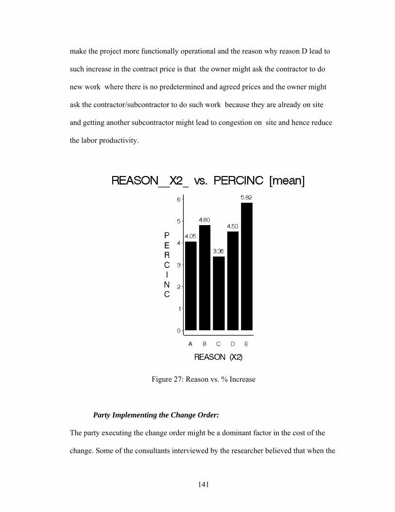
141

make the project more functionally operational and the reason why reason D lead to

such increase in the contract price is that the owner might ask the contractor to do

new work where there is no predetermined and agreed prices and the owner might

ask the contractor/subcontractor to do such work because they are already on site

and getting another subcontractor might lead to congestion on site and hence reduce

the labor productivity.

Figure 27: Reason vs. % Increase

Party Implementing the Change Order:

The party executing the change order might be a dominant factor in the cost of the

change. Some of the consultants interviewed by the researcher believed that when the

142

work assigned in the change order is executed by the subcontractor, the cost will be

higher as the contractor will add profit to the subcontractor price and submit to the

owner.

Figure 28 shows that most of the time the contractor is the one executing the change

order and this might be due to the fact of saving the money and self perform the work.

Figure 28: Frequency of Party Factor

Figure 29 shows that the percent increase can reach to an average of 6.32% when the

subcontractor is performing the change compared to an average of 4.03% when the

contractor is the one executing the change order.

C= Contractor S= Subcontractor

143

Figure 29: Party vs. % Increase

Approved Change Order Hours (APPCO):

As discussed in Chapter three, and reference to equation 13, this factor is measured

as:

100)


orderchangeeachforissuedorderchangeApproved …………………Eq14

As shown in figure 30, the data range of the of the approved change order hours are

from 0 to 100%. This factor depends on the way the change order is compensated; if

it is compensated as a lump sum, there is no information on the breakdown of the

change order cost by the hours used to perform the change order. If the change order

144

is compensated as unit price, the hourly rate and the expected hours expended are

sometimes recorded. Time and material basis way of compensation is the only

detailed method that states in detail form the daily reports the number of hours

expended is the time and material basis.

Figure 30: Frequency of Approved Change Order Hours in % Factor

Figure 31 shows the approved change order hours vs. the percent increase. As for the

range of the percent increase of the change order cost it ranges from 4.667 % to

16.21% increase in the contract price.

145

Figure 31: Approved Change Order Hours in % vs. % Increase

Work Stoppage:

It is not uncommon that the contractor has to stop the work when a change order is

issued. Figure 32 shows the frequency of the work stoppage in the sample of projects

studied. Work stoppage does not occur very frequently and this is due to the fact that

according to the contract clauses of most construction contracts, the contractor has to

continue the work and express his intent to file a claim if he is not satisfied with the

owner decision for the changed work whether for money or time compensation.

That might explain figure 33 where the price difference is not striking when the work

stoppage is present versus when there is no stoppage. If the contractor stopped the

work he will be violating the contract agreement and he will do the stoppage of the

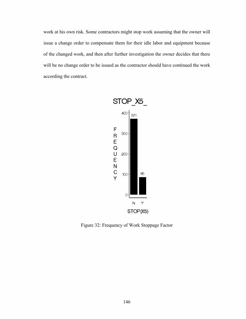
146

work at his own risk. Some contractors might stop work assuming that the owner will

issue a change order to compensate them for their idle labor and equipment because

of the changed work, and then after further investigation the owner decides that there

will be no change order to be issued as the contractor should have continued the work

according the contract.

Figure 32: Frequency of Work Stoppage Factor

147

Figure 33: Work Stoppage vs. % Increase

Restricted Access:

Change resulted in restricted access for both the work area and the nearness of other

trades components' will definitely affect the cost of the change order. Restricted

access negatively affects the productivity of the labor as they expend more hours to

do their work.

As shown in figure 34 restricted access did not occur frequently in the projects

studied. However when this problem emerged in the project, the percent increase in

the contract price can reach an average of almost 5 % as shown in figure 35. This

might be due to the reduced productivity of the labor when there is a restricted access

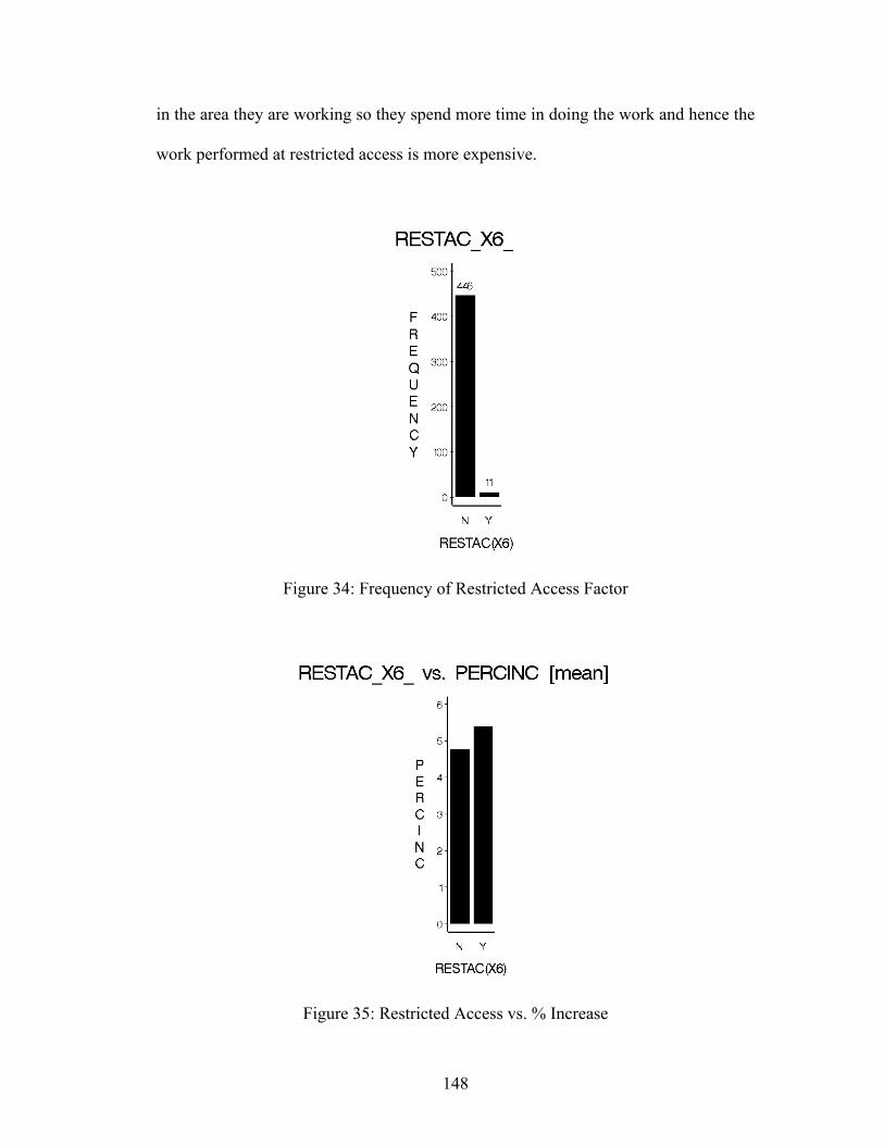
148

in the area they are working so they spend more time in doing the work and hence the

work performed at restricted access is more expensive.

Figure 34: Frequency of Restricted Access Factor

Figure 35: Restricted Access vs. % Increase

149

Change Order Expended as Credit (addition or deletion)/ Rework/Idle:

Change orders issued to compensate the contractor can be for extra work or work that

has to be removed and redone or for idle labor and equipment due to the changed

work.

Figure 36 shows that most of the change orders issued are expended as credit work,

and then rework comes second.

Figure 37 shows that the most increase in the contract price is when the labor is idle

with an average of 6.19%. This might be due to the fact that when the contractor is

experiencing idle labor he is putting himself in a risk of losing them to another project

and they might become unavailable when the work is resumed. The lack of

availability of labors might make the contractor hire labor with a higher hourly rate so

as not to put his project in the risk of getting delayed and hence pay liquidated

damages.

The second most expensive is the rework. The labor productivity declines when they

are redoing the work. The rework process is elaborated in the figure 38 where it

shows how the labor productivity and learning curve decline when they redo the

work.

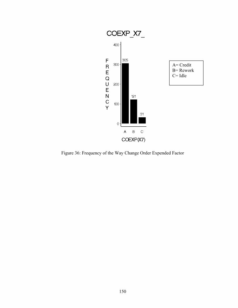
150

Figure 36: Frequency of the Way Change Order Expended Factor

A= Credit B= Rework C= Idle

151

Figure 37: Way Change Order Expended vs. % Increase

Figure 38: Rework Process (Robinson, 2003)

152

The Way the Change Order Compensated:

The way the change order was compensated might influence the price of the change

order. Figure 39 shows that most of the times the change is expended as time and

material basis. This might be due to the fact that according to the time and material

basis method of compensation, the labor, equipment and material compensation will

be derived from the actual daily reports and invoices for extra materials if any. This

might be explained by figure 40 where the average increase in the contract price is the

least if compensated as time and material basis.

The least common way of compensating the change order is the lump sum method

where the contractor submits a price without a break down of the costs incurred due

to the change order Agreement may be difficult to be reached on what is the direct

cost and what would be paid by the contractor out of his overhead and fee. As shown

in figure 40 the compensation for change orders compensated as lump sum is the

most expensive and can increase the contract price to an average of 6.86%.

153

Figure 39: Frequency of the Way Change Order Compensated Factor

Figure 40: Way Change Order Compensated vs. % Increase

A= Lump sum B= Time & Material Basis C= Unit Price

154

Extension:

As previously discussed in Chapter 3, and reference to equation 15, this factor is

measured as:

100)


orderchangeeachforcontractorthetoentitledextensionofDays

….Eq.15

Change orders that provide the contractor entitlement to time extension do not

necessarily provide entitlement for an increase in the contract price as some changes

are excusable but non-compensable delays.

Granting time extensions depends whether this item is a controlling work item

(critical activity) or not. As shown in the figure 41 the time extension ranges from an

average of 1.5% to 31 % as measured by the above equation.

As shown in figure 42, the price increase when extension is present is mostly an

average of 5% to 8%, however when the extension exceeded 25%, the price increase

jumps to over 20%. This last point of 31.5% extension is eliminated from the model.

155

Figure 41: Frequency of Extension Factor in %

Figure 42: Extension vs. % Increase

156

Change Order Work Season:

Most construction contracts clearly give direction to the contractor on studying the

time of the year that the work will be performed and identify the change clauses and

the potential reason for issuing a change order. In such changes clause, the owner

states what the situations that are considered “Changed site conditions”.

Accordingly, contractors need to study the project and their expected start date of

construction. Contractors might mistakenly assign their resources and duration based

on the time of bid preparation not the time of the construction.

Contractors should put some contingency in their duration or cost for any unexpected

conditions like rain for example. A contractor who is studying a bid and knows that

the project area is experiencing continuous rain during the lifetime of the project has

to increase his cost and duration to account for this problem. Some contractors

believes that adding a contingency of time and cost to account for such risks might

put them in a condition of losing the bid. That’s why in many situations the

contractors asks for compensation for a rainy days and in most cases the owners

rejects their request and does not provide entitlement whether for time or money.

As shown in the figure 43, this problem of different seasons does not occur a lot in

the project studied as most owners are strict in terms of defining changed site

conditions and that explains figure 44 of how there is almost no cost difference

between changed season and work done at the same season.

157

Figure 43: Frequency of Season Factor

Figure 44: Season vs. % Increase

158

Stacking of Trades:

The problem of stacking of trades occurs when the change orders force the

contractor/subcontractor to work in an area where another contractor is already

working. This leads to congestion in the site and such congestion affects the mobility

of labor while doing their work and hence reducing their productivity.

As shown in the figure 45 this problem did not occur frequently in the projects

studied and when it appears, it does not increase the contract price as shown in figure

46. This factor will be eliminated from the model as few observations were recorded

when stacking of trades occur.

Figure 45: Frequency of Stacking of Trade Factor

159

Figure 46: Stacking of Trade vs. % Increase

4.2.1.2 Piping Model The main aim of this study is to define and quantify the effects of various attributes

that contribute to the productivity loss of the piping operation explained in Chapter 3.

Both the owner and the contractor-contributed factors will be studied to aid both

parties in quantifying the expected productivity loss. The owner will only be

interested in factors that he is responsible for to compensate the contractor for

productivity loss.

160

As discussed in Chapter 3, and reference to equation 16, the response is measured as:

Loss of Productivity (%) =

oductivityBaseline



ji

ji

Pr

Pr *

−

−

………………………Eq.16

*Baseline Productivity: It is the average best productivity that the contractor

encounters during the periods that were not impacted by the change order.

There are fifteen possible predictors defined in Chapter 3 that have been selected to

predict the productivity loss of piping work that are attributed to both the owner and

the contractor. In addition, two way interaction has been carried between each

variable and the other and that totaled at the start of the model with 225 possible

predictors (284 after coding the qualitative variables) to predict the outcome; %

productivity loss of the piping work.

The distribution of the productivity loss is shown in figure 47. Database collected

from 16 projects that consists of 542 data points for the piping work is used in this

research. Each data point represents productivity from one structure to another in

each project. As previously motioned, productivity is tracked for all the piping work

in each project and measured from one structure to another as explained in Chapter 3.

As shown the productivity loss “PRLOSS” factor ranged from -87% to 470%. A

negative “PRLOSS” means a productivity that exceeds the average best productivity

that the contractor achieves during the lifetime of the project.

161

Figure 47: Distribution of the Response Variable "PRLOSS"

Time Factor:

As shown in figure 48 the data were collected for piping activities from the start till

the end of the project. Reference to equation 17, the timing factor is measured as:

)( )( ) (

daysprojecttheofdurationOriginaldaysproceedtoNoticeStoSfromworkofdateStart ji −

………….…..….Eq. 17

The timing factor can be more than 100% when the project is extended beyond the

target completion date.

162

Figure 48: Frequency of Time Factor in %

As shown in the figure 49 below, the productivity loss is higher in the first 10% of the

job, with an average productivity loss of 67%, and this is due to the learning curve

theory where at the first 10% the labor are mobilizing their equipment and getting

used to the site. Similarly the last 10% of the work the productivity loss went up to

36% when they are working in the punch list and the productivity drops while

finishing up the work (Thomas, 1995b).

When the project exceeded the as planned project completion date (Time

factor>100%), the productivity loss increases dramatically and this is due to the fact

that the contractor did not put such extension of time into consideration when they

were creating their resource allocation. Extension of time might be expended for

163

credit work whether addition or deletion and the contractor might not have the labor

to do this work, or they are waiting for materials to be delivered and hence the

productivity loss decreases. It as well can be extended for rework the activities that

have been previously done, and as mentioned before, the rework scenario can

negatively affect the productivity rate of the labor. After they got the instructions for

the changed work, it is shown that the productivity loss went down again.

Figure 49: Time in % vs. % Productivity Loss

Rain:

As stated in Chapter 3, the researchers had an assumption in this study that a rainy

day is considered excusable but non-compensable delay, which means that the

164

contractor will be waived from paying liquidated damages due to the delay for this

day; however he won’t be paid any for idle labor, or equipment.

The consecutive day of a rainy day will still impact the contractor’s work as the site

will still be wet. Similarly if the work was performed and then a rainy day hindered

the work between two structures, then piping work between the two structures resume

after rain.

As shown in the figure 50, most of the data collected were not affected by rain.

Figure 50: Frequency of Rain Factor

Figure 51 shows the effect of the rain on the productivity loss. When rain occurs just

before the piping work between two structures starts, the productivity loss is an

A=Rain During work B= Rain just before the work starts C= No rain

165

average of 18%. The productivity loss reaches 133% when the rain is encountered

during the work and this is due to the fact that the site is still wet and the piping

excavation and laying operation is affected especially that they might meet need to

redo some of the pipe previously laid and damaged by rain. Also, they will have to

restart their learning curve especially that they stopped the previous day due to heavy

rains.

Figure 51: Rain vs. % Productivity Loss

Dewatering Problem:

Almost every activity in heavy construction projects needs to be performed in such a

way that rain water and ground water will not affect the construction operation. The

A=Rain During work B= Rain just before the work starts C= No rain

166

contractor who ignores such need will be bogged down in costly, time-consuming,

and unnecessary drying activities.

As shown in figure 52, most of the data collected were for projects that did not have

dewatering problem. When the dewatering problem exists, the productivity loss can

reach up to 125% on average as shown in figure 53.

Figure 52: Frequency of Dewatering Factor

167

Figure 53: Dewatering vs. % Productivity Loss

Conflicts /Unforeseen Condition:

Conflicts are commonly encountered in heavy construction projects and that might be

due to design errors or omissions. When the contractor encounters a conflict on site

they have to report it to the owner and wait for direction on how to proceed. The

owner representative might direct them to relocate the pipe or remove the

obstructions encountered to continue the pipe laying operations. All of that will lead

to an increase in the productivity loss of the contractor’s labor.

When the contractor faced a conflict during the pipe laying operation as shown in

figure 54, the productivity loss can reach up to 110% on average as shown in figure

55.

168

Figure 54: Frequency of Conflict Factor

Figure 55: Conflict vs. % Productivity Loss

169

Rework:

As previously discussed, rework negatively affect the productivity. Rework can be

due to faulty construction by the contractor or as a part of the owner changes.

Reference to equation 18, rework factor is measured as:

100)

( XStoSfromspenthoursmanTotal

StoSfromreworkinspenthoursManji

ji

−− ……………………………..Eq. 18

There is few data collected where rework was encountered as shown in figure 56.

Figure 57 shows how the percentage of rework, as measured by the above equation,

vs. productivity loss distribution is mound shape which means that the productivity

loss increase till a certain level of rework percentage till reach a maximum then drops

again and this might be due to the fact that labor got acquainted with the work being

redone and they catch up with their learning curve.

170

Figure 56: Frequency of Rework Factor (in %)

Figure 57: Rework vs. % Productivity Loss

171

Quantity Installed:

The quantity of the piping installed from one structure to another affects the

productivity. A crew who are used to install a certain linear footage per day might not

be as productive if they installed a lesser quantity than what they are used to and

especially if it is a changed work. It is not surprising to find that the work bid at a

certain productivity rate may take 2-4 times more work hours than when it is done as

a changed work (Thomas, 1995b).

Reference to equation 19, this factor is measured as:

100)

( XprojecttheforquantitypipeinstalledTotalStoSfromquatnitypipeInstalled ji …………………………Eq. 19

The data collected range is shown in the figure 58. In most of the projects studied,

the quantity installed from one structure to another as measured by equation 30 is

1.5%.

172

Figure 58: Frequency of % Quantity Installed

As shown in figure 59, the greater the quantity installed form one structure to another,

the better the productivity. A negative productivity loss means that the contractor

achieved a productivity higher than average. The data in figure 59 are supported by

the learning curve theory and the economy of the scale. Economy of the scale is

defined as “Reduction in cost per unit resulting from increased production, realized

through operational efficiencies. Economies of scale can be accomplished because as

production increases, the cost of producing each additional unit falls”.

173

Figure 59: %Quantity Installed vs. % Productivity Loss

Trench Box:

The use of the trench box is a requirement by the OSHA according to the depth of the

excavation and should be specified as part of the contract. The use of the trench box

in the pipe laying operation affects the productivity of the labor and this is due to the

nature of trench box installation as the time to install the trench box might exceeds

that for the trench excavation and pipe laying.

As shown in the figure 60, most of the data collected are without trench boxes.

However as shown in the figure 61, the productivity loss encountered when a trench

box is used can reach up to 100%. . The efficient contractor should have an enough

quantity of trench boxes so that at least one stack is in place while another is moved

174

around in front. In this way, pipe laying will not be stopped during the protective

work. If the site is wet, the production rate of the excavation, trench box installation

and pipe laying will be negatively affected.

Figure 60: Frequency of Trench Box Factor

175

Figure 61: Trench Box vs. % Productivity Loss

Pipe Diameter:

The pipe diameter is measured in mm. Figure 62 shows the pipe diameter installed in

the projects studied and they are mainly: 152, 203, 254, 305, 450, 600, 750, 900,

1200, 1350, and 1500 mm.

176

Figure 62: Frequency of Pipe Diameter Factor

As shown in figure 63, the smaller the pipe diameter the higher the productivity loss.

This might be attributed to the fact that the smaller diameter pipes, 152mm, 203mm,

254, and 305mm were for sanitary sewer pipes. Sanitary Sewer pipes must be laid at

the bottom beneath the storm water, and potable water pipes. This depth requirement

might affect the productivity as the deeper the excavation, the more conflicts or

unforeseen condition might be encountered and the higher the chance of getting close

to the water table which might be more effort to keep the trench dry.

177

Figure 63: Pipe Diameter vs. % Productivity Loss

Pipe Material:

The pipe material might play a role in the pipe laying productivity. The weight of the

pipe is a function of how the labor will handle the pipe and lay it in the trench as well

the type of bedding used. Figure 64 illustrates how the type of the material affect the

type of bedding used and hence affects the productivity of the piping work activities.

This might be attributed to the fact that PVC pipes are mainly used for sanitary sewer

pipes. Sewer pipes are laid beneath the storm water and potable water pipes and there

are strict guidelines about the horizontal and vertical separation of the sanitary sewer

from other types of pipes.

178

Figure 64: Types of Stone Bedding (A J Mccormack & Son, 2006)

Figure 65 shows the main types of pipes that are installed in the projects under study

and they are

A. PVC

B. Corrugated Metal Pipe (CMP)

C. Reinforced concrete pipes (RCP)

Granular material - 10mm single size or 14-5mm graded

Selected Fill or Granular material

Selected Fill - no stones over 40mm, no lumps of clay over 100mm, no organic or frozen material

Bedding detail for flexible pipes (Plastic) Bedding

detail for rigid pipes (Clayware)

179

Figure 65: Frequency of Pipe Type Factor

As shown in figure 66, when PVC pipes are used, the productivity loss was the

highest, followed by concrete pipes and the least is the CMP. This might be attributed

to the fact that PVC pipes are mainly used for sanitary sewer pipes. Sewer mains that

are laid in the vicinity of existing or proposed pipelines, and that are designated to

carry water or reuse water (wastewater effluent) shall meet the horizontal and vertical

separations as follows (City of Melbourne Specs): “As for the horizontal separation

sewer mains shall be located at least 10 feet horizontally from water mains or reuse

water (unless used for unrestricted public access) and three (3) feet horizontally or

five (5) feet center to center whichever is greater from pipes carrying reuse water

used for unrestricted public access. The distance shall be measured from inside edge

of pipe. When local conditions prevent a horizontal separation of 10 feet, a sewer

A= PVC B=CM C=RCP

180

main may be laid closer to a pipe carrying water or reuse water provided that the

bottom of the water main is at least 18 inches above the top of the sewer pipe and the

water main is laid in a separate trench. As for the vertical separation, sewer mains

shall be laid to provide a separation of at least 18 inches between the bottom of the

water main and the top of the sewer”.

Productivity losses in concrete pipes can reach an average of 38%. This might be

attributed to the weight of the pipe and the handling precautions that the labor need to

take into account while laying the pipe.

Figure 66: Pipe Type vs. % Productivity Loss

A= PVC B=CM C=RCP

181

Work Started As Planned/ Delayed:

Whether the activity started at its planned time of the year or not might affect the

productivity rate of the labor. This is an important factor especially when the work

requires certain types of labor and an owner caused delay can put the contractor in a

risk of finding the skilled labor at the suitable time.

As shown in figure 67, most of the time in the projects studied the work started as

planned. The productivity loss is considerably higher when the work is delayed than

the planned start date and it can reach up to 70% loss as shown in figure 68.

Figure 67: Frequency of Start of Work Factor

182

Figure 68: Start of Work vs. % Productivity Loss

Location:

In most of the data collected, the work was performed in the planned location as

shown in figure 69. Changes in location might involve remobilization of labor and

equipment from one area to another and that will affect the productivity of the labor

as well as their learning curve. That explains the jump in the productivity loss of an

average of 60% when there is a change in location versus 32% when the work is done

at the same location of the bid as shown in figure 70.

183

Figure 69: Frequency of Location Factor

Figure 70: Location vs. Productivity Loss

184

Design Accuracy:

Changes in the design whether to correct errors and omissions or to account for

unforeseen condition or other conditions are inevitable in any construction project.

As previously discussed there are main five main reasons for why change orders are

issued as shown in figure 71 and they are:









185

Figure 71: Frequency of the Design Factor

As shown in figure 72, most of the changes issued in the piping work are due to

reason B that accounts for unforeseen condition. This is a problem that most of the

heavy construction projects contractors and owners face. This can be due to several

reasons, It might be due to the fact the owner might have rushed to the design without

studying the area to have the project out for bid and the contractor to start on the

construction phase. Several other reasons might be the cause of such high frequency

of occurring changes due to unforeseen condition, but definitely the owner needs to

pay more attention to why these types of change order occur that often.

186

Figure 72: Design vs. % Productivity Loss

Material:

The contractor has to make sure that the material required for the project has to be

delivered on time and according to contract specifications. Late material delivery or

materials not specified in the bids will put the contractor in a risk of delay and

productivity loss by his labor. As discussed in Chapter three, this factor is measured

as:

A. Not according to the project specs.

B. Late material delivery

C. No material problem

187

As shown in figure 73 most of the times there was no material problem. However as

shown in figure 74, when the materials are not according to the project specifications,

the productivity loss can reach an average of 128%, and when the materials are

delayed very few data were collected when this problem occurred. When this problem

occurs the productivity loss can reach an average of 110%. When there is no material

problem there is still a loss which means that there is another factor contributing to

the loss when there is no materials problem.

Figure 73: Frequency of Material Factor

A= Not according to the project specs. B=Late material delivery C=No material problem

188

Figure 74: Material vs. % Productivity Loss

Accident on Site:

As shown in figure 75, most of the projects studied did not encounter accidents and

when accidents on site occurred, they are caused by the contractor resources. Thus the

factor for owner equipment and third party damage will be eliminated from the study.

189

Figure 75: Frequency of Accident Factor

As shown in Figure 76, when there is an accident caused by the contractor’s

resources, the productivity loss can reach up to 129%.

Figure 76: Accident vs. % Productivity Loss

A=Accidents caused by contractor’s resources D= No accident

190

4.2.2 Data Visualization

Scatter plots were developed between each of the independent variables and the

dependant variable y. In addition, two way interactions between the predictor

variables is examined against the dependant variable in each study; namely the

change order study and the loss of productivity study. The main point is to detect if

there is a trend, either positive or negative, and as well to check the distribution of the

data whether linear, quadratic, or other. If the slope is straight then the variable will

be eliminated.

The following figures 77-81 are samples of scatter plots for different variables.

As shown in figure 77 of time vs. percent increase there is an increasing trend of time

and percent increase, the later the change order is issued the greater the percent

increase in the contract price due to change. The scatter plot as well shows that there

are outliers that will be removed from the study which are the points at time =350%

due to low frequency of occurrence so it considered an outlier.

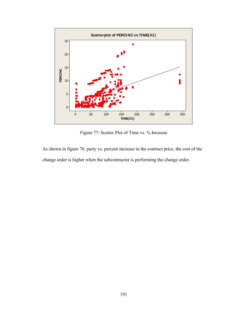
191

TIME(X1)

PER

CINC

350300250200150100500

25

20

15

10

5

0

Scatterplot of PERCINC vs TIME(X1)

Figure 77: Scatter Plot of Time vs. % Increase

As shown in figure 78, party vs. percent increase in the contract price, the cost of the

change order is higher when the subcontractor is performing the change order.

192

PARTY(X3)

PER

CINC

1.00.80.60.40.20.0

25

20

15

10

5

0

Scatterplot of PERCINC vs PARTY(X3)

Figure 78: Scatter Plot of Party vs. % Increase

Similarly as shown in figure 79, the productivity loss decreases with time; a trend

which is explained by the learning curve theory.

0=Subcontractor 1=Contractor

193

TIME(X1)

PRLO

SS

300250200150100500

400

300

200

100

0

-100

Scatterplot of PRLOSS vs TIME(X1)

Figure 79: Scatter Plot of Time vs. % Productivity Loss

As shown in figure 80, rain during work factor vs. productivity loss, the productivity

loss of piping increases when rain is encountered during work between two

structures.

As shown in figure 81, dewatering factor vs. productivity loss, the productivity loss of

piping increases when dewatering problem is encountered.

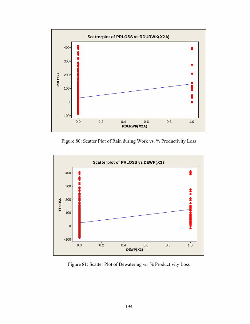
194

RDURWK(X2A)

PRLO

SS

1.00.80.60.40.20.0

400

300

200

100

0

-100

Scatterplot of PRLOSS vs RDURWK(X2A)

Figure 80: Scatter Plot of Rain during Work vs. % Productivity Loss

DEWP(X3)

PRLO

SS

1.00.80.60.40.20.0

400

300

200

100

0

-100

Scatterplot of PRLOSS vs DEWP(X3)

Figure 81: Scatter Plot of Dewatering vs. % Productivity Loss

195

4.3 Model Building

4.3.1 Model without Interaction

As discussed in Chapter 3, two ways interaction will be performed between each of

the independent variables. The researchers first developed a model without the

interaction variables to check how the “main effects” will be able to determine the

variation in the dependent variable so as to have a simpler model.

4.3.1.1 Change Order Model

The model building procedures discussed in Chapter 3 were followed and the

following model was achieved:

PERCINC =

1.13 + 0.0381 TIME(X1) - 0.206 REASON (X2A) + 0.136 REASON (X2B)

- 0.88 REASON (X2C) - 0.532 REASON (X2D) - 2.84 PARTY(X3)

+ 0.0629 APPCO (X4) - 1.63 STOP(X5) - 1.19 RESTAC(X6)

+ 0.530 COEXP(X7A) + 1.28 COEXP(X7B) + 1.17 COCOMP(X8A)

- 1.38 COCOMP (X8B) + 0.012 EXT (X9) + 2.44SEASON(X10)…….Eq. 23

Table 11 shows the P-value for the predictor variables. Variables are considered to be

significant if the P-value is less than α (0.05). As shown in the tables below the only

statistically significant variables are time and the party executing the change whether

contractor or subcontractor. The standard deviation (S) = 3.78729 with R-Sq = 38.0%

and R-Sq (adj) = 35.2%. The coefficient of determination R2 is very low; it means

196

that only 35% of the variability of the % increase in the contract price due to the

change order is explained by the predictor variables thus this model can’t be relied

upon for future prediction of the percent increase of contract price due to change

orders. Such low value of R2 might be an indication that there are not enough

variables to explain the variation of the response variable, thus interaction terms

between each of the predictor variables as discussed in Chapter 3 will be added to the

model.

Table 11: Change Order Model without Interaction Variables

Predictor P VIF

Constant 0.42

TIME(X1) 0.000 1.3

REASON (X2A) 0.836 1.8

REASON (X2B) 0.843 2.7

REASON (X2C) 0.548 1.3

REASON (X2D) 0.518 2.2

PARTY(X3) 0.000 1.1

APPCO (X4) 0.005 1.2

STOP(X5) 0.009 1.5

RESTAC(X6) 0.395 1.1

COEXP(X7A) 0.594 5.6

COEXP(X7B) 0.196 4.8

COCOMP(X8A) 0.077 1.3

COCOMP(X8B) 0.007 1.5

EXT (X9) 0.915 1.1

SEASON(X10) 0.29 1.1

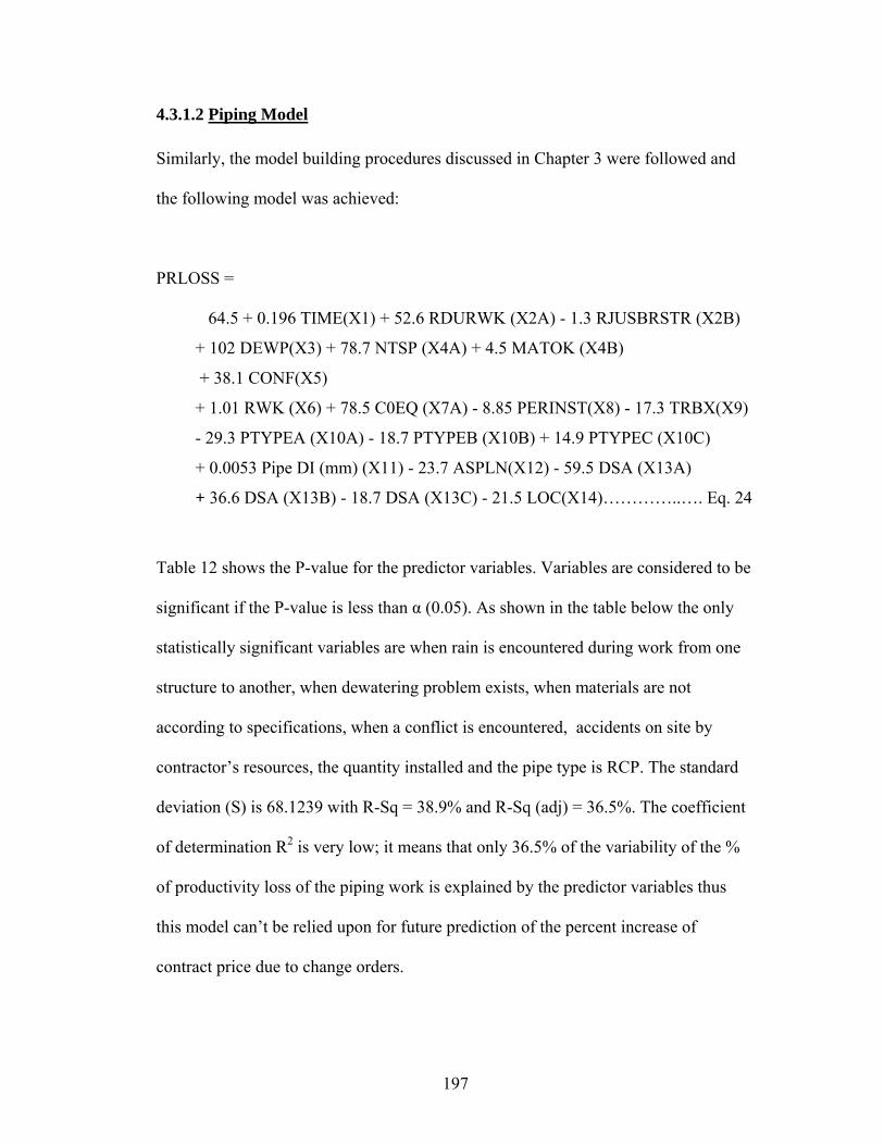
197

4.3.1.2 Piping Model

Similarly, the model building procedures discussed in Chapter 3 were followed and

the following model was achieved:

PRLOSS =

64.5 + 0.196 TIME(X1) + 52.6 RDURWK (X2A) - 1.3 RJUSBRSTR (X2B)

+ 102 DEWP(X3) + 78.7 NTSP (X4A) + 4.5 MATOK (X4B)

+ 38.1 CONF(X5)

+ 1.01 RWK (X6) + 78.5 C0EQ (X7A) - 8.85 PERINST(X8) - 17.3 TRBX(X9)

- 29.3 PTYPEA (X10A) - 18.7 PTYPEB (X10B) + 14.9 PTYPEC (X10C)

+ 0.0053 Pipe DI (mm) (X11) - 23.7 ASPLN(X12) - 59.5 DSA (X13A)

+ 36.6 DSA (X13B) - 18.7 DSA (X13C) - 21.5 LOC(X14)…………..…. Eq. 24

Table 12 shows the P-value for the predictor variables. Variables are considered to be

significant if the P-value is less than α (0.05). As shown in the table below the only

statistically significant variables are when rain is encountered during work from one

structure to another, when dewatering problem exists, when materials are not

according to specifications, when a conflict is encountered, accidents on site by

contractor’s resources, the quantity installed and the pipe type is RCP. The standard

deviation (S) is 68.1239 with R-Sq = 38.9% and R-Sq (adj) = 36.5%. The coefficient

of determination R2 is very low; it means that only 36.5% of the variability of the %

of productivity loss of the piping work is explained by the predictor variables thus

this model can’t be relied upon for future prediction of the percent increase of

contract price due to change orders.

198

Such low value of R2 might be an indication that there are not enough variables to

explain the variation of the response variables, thus interaction terms between each of

the predictor variables as discussed in Chapter 3 will be added to the model.

Table 12: Piping Model without Interaction Variables

Predictor P VIF

Constant 0.000

TIME(X1) 0.057 1.2

RDURWK(X2A) 0.007 1.3

RJUSBRSTR(X2B) 0.945 1.1

DEWP(X3) 0.000 1.3

NTSP(X4A) 0.000 1.3

MATLT(X4B) 0.953 38.5

CONF(X5) 0.001 1.1

RWK (X6) 0.228 1.4

C0EQ(X7A) 0.000 1.2

PERINST(X8) 0.000 1.1

TRBX(X9) 0.473 2.1

PTYPEA(X10A) 0.734 52.5

PTYPEB(X10B) 0.064 1.6

PTYPEC(X10C) 0.04 1.4

Pipe DI (mm)(X11) 0.703 1.7

ASPLN(X12) 0.699 7.1

DSA(X13A) 0.000 2.7

DSA(X13B) 0.385 10.5

DSA(X13C) 0.273 2.4

LOC(X14) 0.365 2.2

199

4.3.2 Model with Interaction

As previously discussed models, the change order model and the piping model

produced a very low R2, which means that such models can’t be used by the owner as

a reliable tool to predict the percent increase in the contract price due to change

orders and the productivity loss of the piping work.

A low R2 , indicates that the predictor variables might not be enough o explain the

response variable. Therefore, Interaction variables will be added between each of the

predictor variables and similarly the procedures for building a model discussed in

Chapter 3 will be followed.

4.3.2.1 Change Order (Total Model)

A database of the change orders that consists of 456 observations (percent increase of

the contract price due to the change order) is used to build the model. The model

developed is as follows:

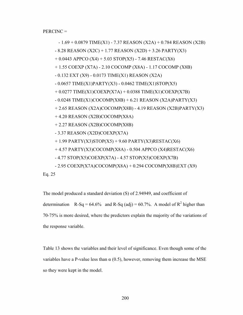
200

PERCINC =

- 1.69 + 0.0879 TIME(X1) - 7.37 REASON (X2A) + 0.784 REASON (X2B)

- 8.28 REASON (X2C) + 1.77 REASON (X2D) + 3.26 PARTY(X3)

+ 0.0443 APPCO (X4) + 5.03 STOP(X5) - 7.46 RESTAC(X6)

+ 1.55 COEXP (X7A) - 2.10 COCOMP (X8A) - 1.17 COCOMP (X8B)

- 0.132 EXT (X9) - 0.0173 TIME(X1) REASON (X2A)

- 0.0657 TIME(X1)PARTY(X3) - 0.0462 TIME(X1)STOP(X5)

+ 0.0277 TIME(X1)COEXP(X7A) + 0.0388 TIME(X1)COEXP(X7B)

- 0.0248 TIME(X1)COCOMP(X8B) + 6.21 REASON (X2A)PARTY(X3)

+ 2.65 REASON (X2A)COCOMP(X8B) - 4.19 REASON (X2B)PARTY(X3)

+ 4.20 REASON (X2B)COCOMP(X8A)

+ 2.27 REASON (X2B)COCOMP(X8B)

- 3.37 REASON (X2D)COEXP(X7A)

+ 1.99 PARTY(X3)STOP(X5) + 9.60 PARTY(X3)RESTAC(X6)

+ 4.57 PARTY(X3)COCOMP(X8A) - 0.504 APPCO (X4)RESTAC(X6)

- 4.77 STOP(X5)COEXP(X7A) - 4.57 STOP(X5)COEXP(X7B)

- 2.95 COEXP(X7A)COCOMP(X8A) + 0.294 COCOMP(X8B)EXT (X9)

Eq. 25

The model produced a standard deviation (S) of 2.94949, and coefficient of

determination R-Sq = 64.6% and R-Sq (adj) = 60.7%. A model of R2 higher than

70-75% is more desired, where the predictors explain the majority of the variations of

the response variable.

Table 13 shows the variables and their level of significance. Even though some of the

variables have a P-value less than α (0.5), however, removing them increase the MSE

so they were kept in the model.

201

Table 13: Change Order Model with Interaction Variables (Total Model)

Predictor P VIF

Constant 0.163

TIME(X1) 0.000 12.6

REASON (X2A) 0.001 13.3

REASON (X2B) 0.331 6.1

REASON (X2C) 0.007 9.5

REASON (X2D) 0.107 6.5

PARTY(X3) 0.000 6.8

APPCO (X4) 0.015 1.3

STOP(X5) 0.002 16.1

RESTAC(X6) 0.001 4.1

COEXP(X7A) 0.089 7.6

COCOMP(X8A) 0.088 7.4

COCOMP(X8B) 0.214 8.7

EXT (X9) 0.173 1.4

TIME (X1) REASON (X2A) 0.110 4.3

TIME (X1) PARTY(X3) 0.000 7.2

TIME (X1) STOP (X5) 0.000 16

TIME (X1) COEXP (7A) 0.003 8.9

TIME (X1) COEXP (7B) 0.000 5.8

TIME (X1) COCOMP (X8A) 0.003 10.8

REASON (X2A) PARTY (X3) 0.003 11.4

REASON (X2A) COCOMP (X8B) 0.061 2.8

REASON (X2B) PARTY (X3) 0.000 6.1

REASON (X2B) COCOMP (X8A) 0.000 3.2

REASON (X2B) COCOMP (X8B) 0.008 6.3

REASON (X2D) COEXP (X7A) 0.003 5.9

PARTY (X3) STOP (X5) 0.038 3.7

PARTY (X3) RESTAX (X6) 0.000 4.9

PARTY (X3) COCOMP (X8A) 0.000 4.6

202

APPCO (X4) RESTAC (X6) 0.136 1.7

STOP (X5) COEXP (X7A) 0.000 4.5

STOP (X5) COEXP (X7B) 0.000 4.0

COEXP (X7A) COCOMP (X8A) 0.008 4.4

COCOMP (X8B) EXT (X9) 0.222 1.7

The second step is to check the linear regression assumptions mentioned in Chapter 3.

To achieve this step four plots are created as shown in figure 82 below:

It is assumed in multiple regression that the residuals (predicted minus observed

values) are distributed normally (i.e., follow the normal distribution).

For moderate to large samples, the simplest way is to determine whether the data

violate the assumption of the normality is to construct a relative frequency histogram

and the normal probability plot. If the distribution is mound shape, and then the

inferences derived from the regression analysis are valid. If no normality is detected,

variable transformation can be performed to enhance its performance in the model.

As shown in the normal probability plot and the residual histogram the data seems to

follow a normal distribution. In addition, a constant variance is assumed in the linear

regression this means that the residual versus fitted values are not following a trend

either positive or negative.

203

As shown in the residual versus fitted value the data seems to follow a trend (fan<)

from 0 to 5% percent increase of contract price due to the change order and another

trend (fan>) when the percent increase exceeded 5%. In other words, the variance is

not constant which means that we are violating an important assumption of linear

models.

Figure 82: Residual Plots for PERCINC (Total Model)

The data were divided into two sets; the first set is for observations with a percent

increase in the contract price less than 5% and the second set is for data with percent

increase more than 5%. This limit of 5% is supported previous research by Adrian

1987 and Hanna 1999a,b as most construction projects are expected to experience

Residual

Per

cent

1050-5-10

99.9

99

90

50

10

1

0.1

Fitted Value

Res

idua

l

20151050

10

5

0

-5

-10

Residual

Freq

uenc

y

630-3-6-9

60

45

30

15

0

Observation Order

Res

idua

l

300250200150100501

10

5

0

-5

-10

Normal Probability Plot of the Residuals Residuals Versus the Fitted Values

Histogram of the Residuals Residuals Versus the Order of the Data

Residual Plots for PERCINC

204

change orders that increase the contract price by 5% and more than 5% is a problem

that might lead to claims and disputes; a problem that causes loss of money and time

to both parties.

Two models are created as follows:

The first to predict the percent increase in the contract price due to

change orders when the cumulative increase in the contract price due

to change orders is less than 5%.

The second to predict the percent increase in the contract price due to

change orders when the cumulative increase in the contract price due

to change orders is more than 5%.

4.3.2.2 Change Order Model for Percent Increase More Than 5%

In order to meet the constant variance assumption, transformation of the response

variables, discussed in Chapter 3, is performed. Inverse square root transformation for

the percent increase is performed. A sample of the data used to build the model is

shown in Appendix C.

The model achieved is as follows:

205

PERCINC^-0.5 =

0.343 + 0.000865 TIME(X1) - 0.0539 REASON (X2A) + 0.0566 REASON

(X2B) - 0.114 REASON (X2D) + 0.0315 PARTY(X3)

- 0.00137 APPCO (X4)

- 0.241 RESTAC(X6) + 0.0318 COEXP(X7A) + 0.0462 COEXP(X7B)

+ 0.0580 COCOMP(X8A) + 0.106 COCOMP(X8B) - 0.00978 EXT (X9)

+ 0.000501 TIME(X1)REASON (X2A) + 0.000018 TIME(X1)APPCO(X4)

+ 0.00239 TIME(X1)RESTAC(X6) - 0.000277 TIME(X1)COEXP(X7A)

- 0.000706 TIME(X1)COEXP(X7B) - 0.00111 TIME(X1)COCOMP(X8A)

- 0.000946 TIME(X1)COCOMP(X8B) - 0.0513 REASON (X2B)COEXP(X7A)

- 0.0567 REASON (X2B)COCOMP(X8B) + 0.0133 REASON (X2B)EXT (X9)

- 0.102 REASON (X2D)PARTY(X3) + 0.0834 REASON (X2D)COEXP(X7A)

+ 0.0961 REASON (X2D)COEXP(X7B) + 0.0629 REASON

(X2D)COCOMP(X8A) + 0.0578 PARTY(X3)COCOMP(X8B).................Eq. 26

As shown in table 14, even though some of the variables have a P-value< α (0.05)

which means they are not significant, the researchers included them in the model

because of their significance in the field. The researchers want to rely as well on the

Engineering experience and not only rely on the statistical significance of the

variables. As shown as well most of the variables have low variables of inflation

(VIF) and this is important to make sure that the model is not suffering from

multicollinearity. The literature stated a VIF up to 10; however practically it can

reach up to 100.

When the change order increases the contract price by more than 5%, the most

significant factors that explain the percent increase in the contract price due to change

orders are:

206

• Time,

• Reason of the change (A,B&D),

• Party performing the changed work,

• The way change order is compensated.

• Extension

As for the interaction variables, the most significant interaction of variables that

contribute to the increase in the contract price due to the change order:

• Time and (reason of the change (A), approved change order, restricted

access, the way the change order is expended, and how the change order is

compensated).

• Reason (B) and (change order is expended as credit, change order is

compensated as time and material basis, extension is granted).

• Reason (D) and (party, way the change order is expended, when the

change order is compensated as lump sum).

207

Table 14: P-Values & VIF Change Order model for PERCINC >5%

Predictor P VIF

Constant 0.000

TIME(X1) 0.000 24.4

REASON (X2A) 0.025 8.1

REASON (X2B) 0.000 10.5

REASON (X2D) 0.000 1.5

PARTY(X3) 0.000 3.4

APPCO (X4) 0.069 10.1

RESTAC(X6) 0.032 74.9

COEXP(X7A) 0.161 26.8

COEXP(X7B) 0.032 20.8

COCOMP(X8A) 0.004 12.0

COCOMP(X8B) 0.000 16.8

EXT (X9) 0.002 3.3

TIME (X1) REASON (X2A) 0.006 10.3

TIME (X1) APPCO(X34) 0.006 13.0

TIME (X1) RESTAC (X6) 0.029 75.6

TIME (X1) COEXP (7A) 0.017 11.9

TIME (X1) COEXP (7B) 0.000 12.5

TIME (X1) COCOMP (X8A) 0.000 18.6

TIME (X1) COCOMP (X8B) 0.000 36.0

REASON (X2B) COEXP (X7A) 0.001 10.8


REASON (X2B) EXT (X9) 0.001 3.1

REASON (X2D) PARTY (X3) 0.000 3.9

REASON (X2D) COEXP (X7A) 0.000 5.5

REASON (X2D) COEXP (X7B) 0.000 3.3

REASON (X2D) COCOMP (X8A) 0.001 1.7

PARTY (X3) COCOMP (X8B) 0.000 5.1

208

The number of data points used to create this model is 137 data points. The standard

deviation (S) achieved is 0.0253270, R-Sq = 80.2% and R-Sq (adj) = 75.3%. This

means that 75% of the variability in the response variable, percent increase in the

contract price due to change orders, is explained by the predictor variables.

As shown in figure 83, the normal distribution assumption is checked using the

normality plot and the histogram of the residuals. As for the constant variance

assumption, the data has improved from the first trial (when all the data of the change

order are evaluated in one model for PERCIN from 0-16.5%) and the data are not

following any trends.

Residual

Per

cent

0.080.040.00-0.04-0.08

99.9

99

90

50

10

1

0.1

N 137AD 0.471P-Value 0.241

Fitted Value

Res

idua

l

0.450.400.350.300.25

0.050

0.025

0.000

-0.025

-0.050

Residual

Freq

uenc

y

0.060.040.020.00-0.02-0.04

30

20

10

0

Observation Order

Res

idua

l

130

120

110

1009080706050403020101

0.050

0.025

0.000

-0.025

-0.050

Normal Probability Plot Residuals Versus the Fitted Values


Residual Plots for Y^-.5

Figure 83: Residual Plots for PERCINC >5%

209

4.3.2.3 Change Order Model for Percent Increase Less than 5%

In order to meet the constant variance assumption, transformation of the response

variables is performed for the percent increase. A sample of the data used to build the

model is shown in Appendix C.

The model achieved is as follows:

PERCINC^0.4 =

1.56 + 0.00763 TIME(X1) + 0.365 REASON (X2A) + 0.139 REASON (X2B)


+ 0.00308 APPCO (X4) + 0.354 STOP(X5) - 0.947 COEXP(X7A)

- 0.912 COEXP(X7B) + 0.256 COCOMP(X8A) - 0.519 COCOMP(X8B)

+ 0.00832 EXT (X9) - 0.00699 TIME(X1)REASON (X2A)

- 0.00535 TIME(X1)REASON (X2C) - 0.00535 TIME(X1)REASON (X2D)

+ 0.112 REASON (X2A)APPCO (X4) - 0.480 REASON (X2A)STOP(X5)

- 0.385 REASON (X2B)PARTY(X3) - 0.342 REASON (X2B)STOP(X5)

+ 0.224 REASON (X2B)COCOMP(X8B)

+ 0.679REASON(X2C)COCOMP(X8A)

+ 0.850 REASON (X2C)COCOMP(X8B) - 0.263 PARTY(X3)STOP(X5)

+ 0.175 PARTY(X3)COEXP(X7A) - 0.401 PARTY(X3)COCOMP(X8B)

- 0.164 STOP(X5)COEXP(X7B) + 0.594 COEXP(X7A)COCOMP(X8B)

+ 0.759 COEXP(X7B)COCOMP(X8B)…………………………….……Eq. 27

The number of data points used to create this model is 208 data points The model has

a standard deviation (S ) of 0.25959, R-Sq = 62.9% and R-Sq(adj) = 57%. This

means that only 57% of the variation of the response variable percent increase in the

contract price due to change order is explained by the predictors. This is a

considerably low value of R-Sq (adj), however as supported by the literature most of

210

construction projects experience change orders up to 5% and more than 5% is where

problems of quantification arise.

As shown in table 15, though some of the variables have P-value less than alpha,

which means they are not statistically significant, however from the researchers

experience and the consultants interviewed these variables will be kept in the model.

Most of the variables have a variable of inflation less than 100; a threshold which

above multicollinearity is present. The most significant factors that explain the

percent increase in the contract price due to change orders are:

• Time,

• Reason for the change (A&D),

• Way the change order is expended,

• How the change order is compensated.

As for the interaction variables, the most significant interaction of variables that

contribute to the increase in the contract price due to the change order are:

• Time and the reason of the change (A&D),

• Reason (A) and (approved change order hours)

• Reason (B) and (the party performing the change, and when the change

order is compensated as time and material basis)

• Reason (C) and the way the change order is compensated,

• Party and the when the change order is compensated as time and material

basis

• The way the change order is expended and when the change order is

compensated as time and material basis.

211

Table 15: P-Values & VIF Change Order model for PERCINC <5%

Predictor P VIF Constant 0.000 TIME(X1) 0.000 2.3

REASON (X2A) 0.011 5.2

REASON (X2B) 0.139 6.6

REASON (X2C) 0.413 11.6

REASON (X2D) 0.008 6.5 PARTY(X3) 0.215 8 APPCO (X4) 0.307 1.3

STOP (X5) 0.022 11.6

COEXP(X7A) 0.000 29.3

COEXP(X7B) 0.000 27.3

COCOMP(X8A) 0.000 1.6

COCOMP(X8B) 0.042 49.7

EXT (X9) 0.365 1.2

TIME (X1) REASON (X2A) 0.000 5.4

TIME (X1) REASON (X2C) 0.013 13.6

TIME (X1) REASON (X2D) 0.000 7.2

REASON (X2A) APPCO (X4) 0.008 2.4

REASON (X2A) STOP (X5) 0.022 2.5

REASON (X2B) PARTY (X3) 0.000 7.3

REASON (X2B) STOP (X5) 0.007 6.0


REASON (X2C) COCOMP (X8A) 0.002 2.0

REASON (X2C) COCOMP (X8B) 0.000 3.9

PARTY (X3) STOP (X5) 0.048 7.1

PARTY (X3) COEXP (X7A) 0.133 10.4

PARTY (X3) COCOMP (X8B) 0.000 9.7

STOP (X5) COEXP (X7B) 0.142 2.1

COEXP (X7A) COCOMP (X8B) 0.009 33.0

COEXP (X7B) COCOMP (X8B) 0.001 23.9

212

As shown in figure 84, the normal probability plot and the histogram of the residuals

the data follows a normal distribution, and the residual versus the fitted value the

variance is not following a trend, thus the assumption of constant error is met.

Residual

Per

cent

0.80.40.0-0.4-0.8

99.9

99

90

50

10

1

0.1

N 208AD 0.705P-Value 0.065

Fitted Value

Res

idua

l

2.01.51.00.5

0.50

0.25

0.00

-0.25

-0.50

Residual

Freq

uenc

y

0.450.300.150.00-0.15-0.30-0.45

20

15

10

5

0

Observation Order

Res

idua

l

200180160140120100806040201

0.50

0.25

0.00

-0.25

-0.50



Residual Plots for Y^0.4

Figure 84: Residual Plot for PERCINC<5%

4.3.2.4 Piping Model (Total Model)

A database of the daily productivity of the piping work from one structure to another

that consists of 410 observations is used to build the model.

The final model developed is as follows:

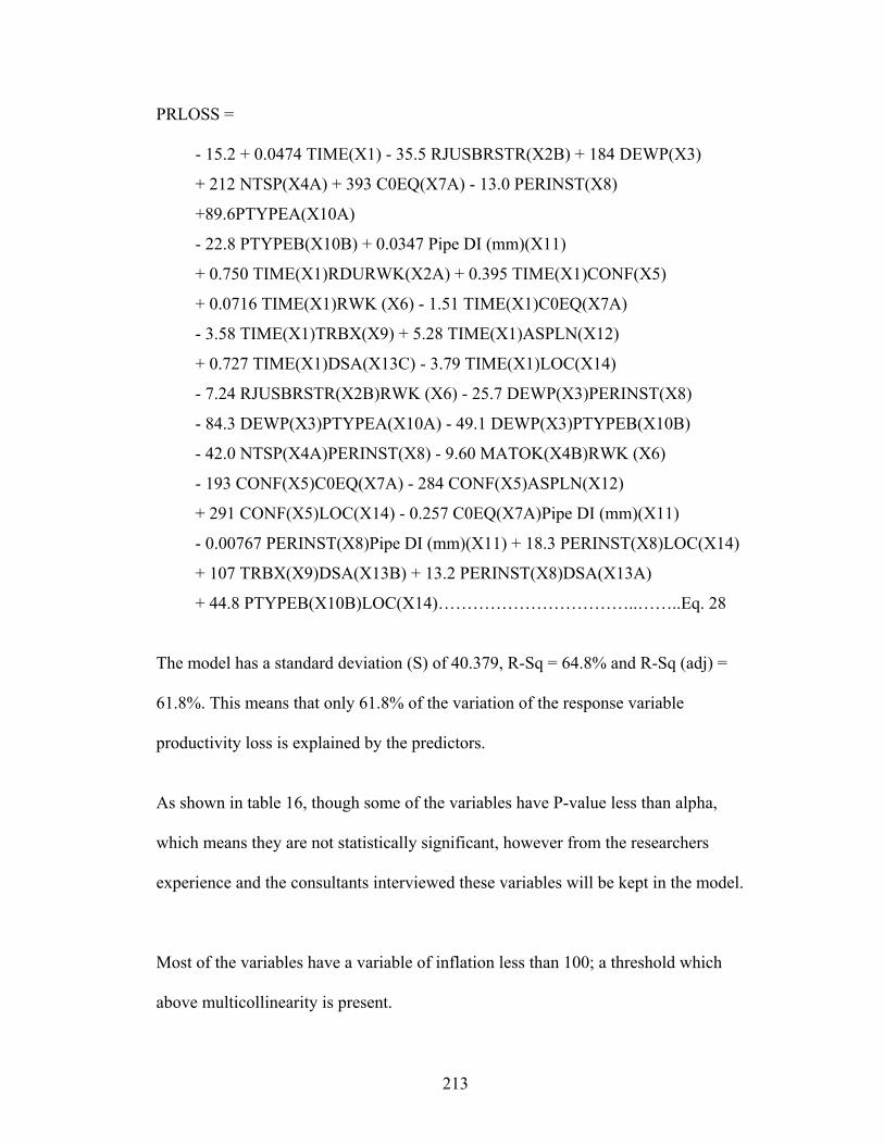
213

PRLOSS =

- 15.2 + 0.0474 TIME(X1) - 35.5 RJUSBRSTR(X2B) + 184 DEWP(X3)

+ 212 NTSP(X4A) + 393 C0EQ(X7A) - 13.0 PERINST(X8)

+89.6PTYPEA(X10A)

- 22.8 PTYPEB(X10B) + 0.0347 Pipe DI (mm)(X11)

+ 0.750 TIME(X1)RDURWK(X2A) + 0.395 TIME(X1)CONF(X5)

+ 0.0716 TIME(X1)RWK (X6) - 1.51 TIME(X1)C0EQ(X7A)

- 3.58 TIME(X1)TRBX(X9) + 5.28 TIME(X1)ASPLN(X12)

+ 0.727 TIME(X1)DSA(X13C) - 3.79 TIME(X1)LOC(X14)

- 7.24 RJUSBRSTR(X2B)RWK (X6) - 25.7 DEWP(X3)PERINST(X8)

- 84.3 DEWP(X3)PTYPEA(X10A) - 49.1 DEWP(X3)PTYPEB(X10B)

- 42.0 NTSP(X4A)PERINST(X8) - 9.60 MATOK(X4B)RWK (X6)

- 193 CONF(X5)C0EQ(X7A) - 284 CONF(X5)ASPLN(X12)

+ 291 CONF(X5)LOC(X14) - 0.257 C0EQ(X7A)Pipe DI (mm)(X11)

- 0.00767 PERINST(X8)Pipe DI (mm)(X11) + 18.3 PERINST(X8)LOC(X14)

+ 107 TRBX(X9)DSA(X13B) + 13.2 PERINST(X8)DSA(X13A)

+ 44.8 PTYPEB(X10B)LOC(X14)……………………………..……..Eq. 28

The model has a standard deviation (S) of 40.379, R-Sq = 64.8% and R-Sq (adj) =

61.8%. This means that only 61.8% of the variation of the response variable

productivity loss is explained by the predictors.





above multicollinearity is present.

214

Table 16: Piping Model with Interaction Variables (Total Model)

Predictor P VIF Constant 0.15 TIME(X1) 0.492 1.3 RJUSBRSTR(X2B) 0.007 1.2 DEWP(X3) 0.000 13.8 NTSP(X4A) 0.000 4.2 C0EQ(X7A) 0.000 16.5 PERINST(X8) 0.004 18.5 PTYPEA(X10A) 0.000 4.5 PTYPEB(X10B) 0.000 1.7 Pipe DI (mm)(X11) 0.008 3.5 TIME(X1)RDURWK(X2A) 0.046 2.6 TIME(X1)CONF(X5) 0.002 1.5 TIME(X1)RWK (X6) 0.000 3.3 TIME(X1)C0EQ(X7A) 0.000 6.2 TIME(X1)TRBX(X9) 0.000 15.1 TIME(X1)ASPLN(X12) 0.000 32.8 TIME(X1)DSA(X13C) 0.029 6.5 TIME(X1)LOC(X14) 0.000 28.5 RJUSBRSTR(X2B)RWK (X6) 0.000 2.2 DEWP(X3)PERINST(X8) 0.001 7.2 DEWP(X3)PTYPEA(X10A) 0.008 4.3 DEWP(X3)PTYPEB(X10B) 0.049 3.3 NTSP(X4A)PERINST(X8) 0.000 3.3 MATOK(X4B)RWK (X6) 0.000 3.5 CONF(X5)C0EQ(X7A) 0.000 2.4 CONF(X5)ASPLN(X12) 0.000 2.9 CONF(X5)LOC(X14) 0.000 5.2 C0EQ(X7A)Pipe DI (mm)(X11) 0.000 8.3 PERINST(X8)Pipe DI (mm)(X11) 0.038 8.6 PERINST(X8)LOC(X14) 0.126 9.2 TRBX(X9)DSA(X13B) 0.001 1.9 PERINST(X8)DSA(X13A) 0.006 21.3 PTYPEB(X10B)LOC(X14) 0.187 2.1

As shown in figure 85, the data follow a normal distribution as shown in the normal

probability plot and the histogram of the residuals.

In the residual versus the fitted value graph, the data seems to be divided into two

sets, the first set of data where there is an enhancement of productivity loss

215

(PRLOSS<0) and the second set of data for those where productivity loss is

encountered (PRLOSS>0).

The main objective is to focus on the data set where productivity loss is encountered

and analyze the factors that contribute to this loss. The researchers will focus only on

the data where productivity loss is encountered (PRLOSS>0).

Figure 85: Residual Plot for PRLOSS (Total Model)

4.3.2.5 Piping Model for PRLOSS>0% Suffered by the Contractor:

The data for productivity loss more than 0 is separated and the procedures listed in

Chapter 3 for model building procedures are followed. A sample of the data used to

build the model is shown in Appendix C.

Residual

Per

cent

100500-50-100

99.9

99

90

50

10

1

0.1

N 410AD 0.754P-Value 0.049

Fitted Value

Res

idua

l

3002001000-100

100

50

0

-50

-100

Residual

Freq

uenc

y

12080400-40-80-120

60

45

30

15

0

Observation Order

Res

idua

l

400350300250200150100501

100

50

0

-50

-100



Residual Plots for PRLOSS

216

The model includes both the contractor and the owner factors that contribute to the

increase in the productivity losses. The owner will issue a change order only for the

productivity loss factors that he is responsible for. Both models are presented to show

the difference between what the contractor usually asks for and what he is entitled to.

Square root transformation is achieved to meet the assumption of constant variance.

The following is the final model produced to quantify the productivity loss of the

piping work.

PRLOSS^0.5 =

9.54 - 0.102 TIME(X1) + 10.2 RDURWK(X2A) - 0.265 RJUSBRSTR(X2B)

+ 6.72 DEWP(X3) + 5.83 NTSP(X4A) + 0.356 CONF(X5) - 0.0855 RWK (X6)

+ 4.96 C0EQ(X7A) - 1.51 PERINST(X8) - 4.84 TRBX(X9)

+ 3.86 PTYPEA(X10A)

- 0.36 PTYPEB(X10B) - 0.00267 Pipe DI (mm)(X11) - 1.12 ASPLN(X12)

+ 3.29 DSA(X13A) - 1.96 DSA(X13B) + 0.20 DSA(X13C)

+ 0.0177 TIME(X1)PERINST(X8) - 0.0652 TIME(X1)PTYPEB(X10B)

+ 0.000053 TIME(X1)Pipe DI (mm)(X11) + 0.0434 TIME(X1)DSA(X13A)

+ 0.0586 TIME(X1)DSA(X13C) - 9.61 RDURWK(X2A)DSA(X13A)

- 3.55 DEWP(X3)PTYPEB(X10B) - 4.47 CONF(X5)C0EQ(X7A)

+ 0.639 CONF(X5)PERINST(X8) - 8.43 CONF(X5)DSA(X13C)

- 0.500 C0EQ(X7A)PERINST(X8) + 11.4 C0EQ(X7A)TRBX(X9)

- 8.70 TRBX(X9)PTYPEA(X10A)

+ 0.00386 PTYPEB(X10B)Pipe DI (mm)(X11)

- 0.00616 Pipe DI (mm)(X11)DSA(X13A)……………………..………Eq. 29

217

The data base used to build the productivity loss model consists of 144 data points

from 12 different projects. The model has a standard deviation of S = 0.953469 R-

Sq = 86.0% R-Sq (adj) = 82.0%.






Analyzing all the productivity loss suffered by the contractor, and including all the

factors that are attributed to both parties, the most significant variables that contribute

to the productivity loss are:

• Time,

• Rain during work,

• When dewatering problem is encountered,

• When the materials are not according to the project specifications,

• Rework,

• When there is an accident caused by the contractor’s resources,

• Quantity installed, and the use of trench box. .

As for the interaction variables, the most significant interaction variables that

contribute to the productivity loss quantification are:

218

• Time and (percent installed, pipe type, time and pipe diameter, when there

is a change order issued for unforeseen conditions).

• When there is a dewatering problem and the pipe type.

• When there is a conflict and (an accident on site due to the contractor’s

resources, the quantity installed).

• Accident on site and (quantity installed, and where trench box is used).

• The use of trench box and the installation of PVC pipe, and

• Finally the use of CM and the pipe diameter.

219

Table 17: P-Values for PRLOSS>0 Suffered by the Contractor

Predictor P VIF Constant 0.000 TIME(X1) 0.000 37.3 RDURWK(X2A) 0.000 6.2 RJUSBRSTR(X2B) 0.685 1.8 DEWP(X3) 0.000 6.5 NTSP(X4A) 0.000 2.1 CONF(X5) 0.461 3.6 RWK (X6) 0.000 2.6 C0EQ(X7A) 0.000 4.9 PERINST(X8) 0.000 20.1 TRBX(X9) 0.000 8.7 PTYPEA(X10A) 0.001 12.4 PTYPEB(X10B) 0.755 26.7 Pipe DI (mm)(X11) 0.008 11.7 ASPLN(X12) 0.455 12 DSA(X13A) 0.001 26.2 DSA(X13B) 0.020 5 DSA(X13C) 0.850 20 TIME(X1)PERINST(X8) 0.000 19.8 TIME(X1)PTYPEB(X10B) 0.000 9.8 TIME(X1)Pipe DI (mm)(X11) 0.000 19.5 TIME(X1)DSA(X13A) 0.000 30.1 TIME(X1)DSA(X13C) 0.002 31.7 RDURWK(X2A)DSA(X13A) 0.000 4.1 DEWP(X3)PTYPEB(X10B) 0.000 4.1 CONF(X5)C0EQ(X7A) 0.000 2.3 CONF(X5)PERINST(X8) 0.000 5.1 CONF(X5)DSA(X13C) 0.000 3.8 C0EQ(X7A)PERINST(X8) 0.009 5.2 C0EQ(X7A)TRBX(X9) 0.000 3.2 TRBX(X9)PTYPEA(X10A) 0.000 12 PTYPEB(X10B)Pipe DI (mm)(X11) 0.000 19.4 Pipe DI (mm)(X11)DSA(X13A) 0.000 21.6

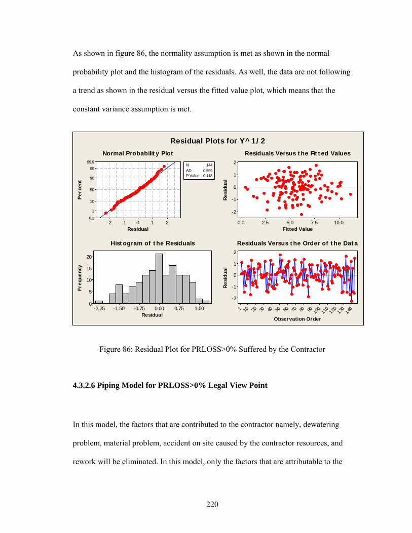
220

As shown in figure 86, the normality assumption is met as shown in the normal

probability plot and the histogram of the residuals. As well, the data are not following

a trend as shown in the residual versus the fitted value plot, which means that the

constant variance assumption is met.

Residual

Per

cent

210-1-2

99.9

99

90

50

10

1

0.1

N 144AD 0.599P-Value 0.118

Fitted ValueR

esid

ual

10.07.55.02.50.0

2

1

0

-1

-2

Residual

Freq

uenc

y

1.500.750.00-0.75-1.50-2.25

20

15

10

5

0

Observation Order

Res

idua

l

140

130

120

110

1009080706050403020101

2

1

0

-1

-2



Residual Plots for Y^1/2

Figure 86: Residual Plot for PRLOSS>0% Suffered by the Contractor

4.3.2.6 Piping Model for PRLOSS>0% Legal View Point

In this model, the factors that are contributed to the contractor namely, dewatering

problem, material problem, accident on site caused by the contractor resources, and

rework will be eliminated. In this model, only the factors that are attributable to the

221

owner will be included. A sample of the data used to build the model is shown in

Appendix C.

Log transformation is achieved to meet the assumption of constant variance. The

following is the final model produced to quantify the productivity loss of the piping

work due to the owner changes.

Log PRLOSS =

2.35 - 0.00560 TIME(X1) + 0.785 RDURWK(X2A) + 0.182 CONF(X5)

- 0.251 PERINST(X8) + 0.348 PTYPEA(X10A) + 0.548 PTYPEB(X10B)

- 0.000694 Pipe DI (mm)(X11) - 0.0712 DSA(X13A) - 0.500 DSA(X13B)

- 0.169 DSA(X13C) + 0.00304 TIME(X1)PERINST(X8)

- 0.0189 TIME(X1)PTYPEB(X10B) + 0.00816 TIME(X1)DSA(X13C)

+ 0.894 RDURWK(X2A)CONF(X5)

- 0.345 RDURWK(X2A)PERINST(X8)……………………….……..Eq. 30

The data base used to build the productivity loss model consists of 88 data points

from 12 different projects. The model has a standard deviation of S = 0.1397 R-Sq

= 76.5%, and R-Sq(adj) = 71.6%.




222



When analyzing only the productivity loss factors that are attributed to the owner, the

most significant factors are:

• Time,

• When rain is during work,

• When there is a conflict encountered,

• Quantity installed,

• The pipe type and diameter.

As for the interaction variables, the most significant interaction variables that

contribute to the productivity loss quantification are:

• Time and the quantity installed,

• Time and pipe type,

• Time and when there is a change in design due to conflicts or unforeseen

conditions, and

• When there is a rain during work and a conflict encountered

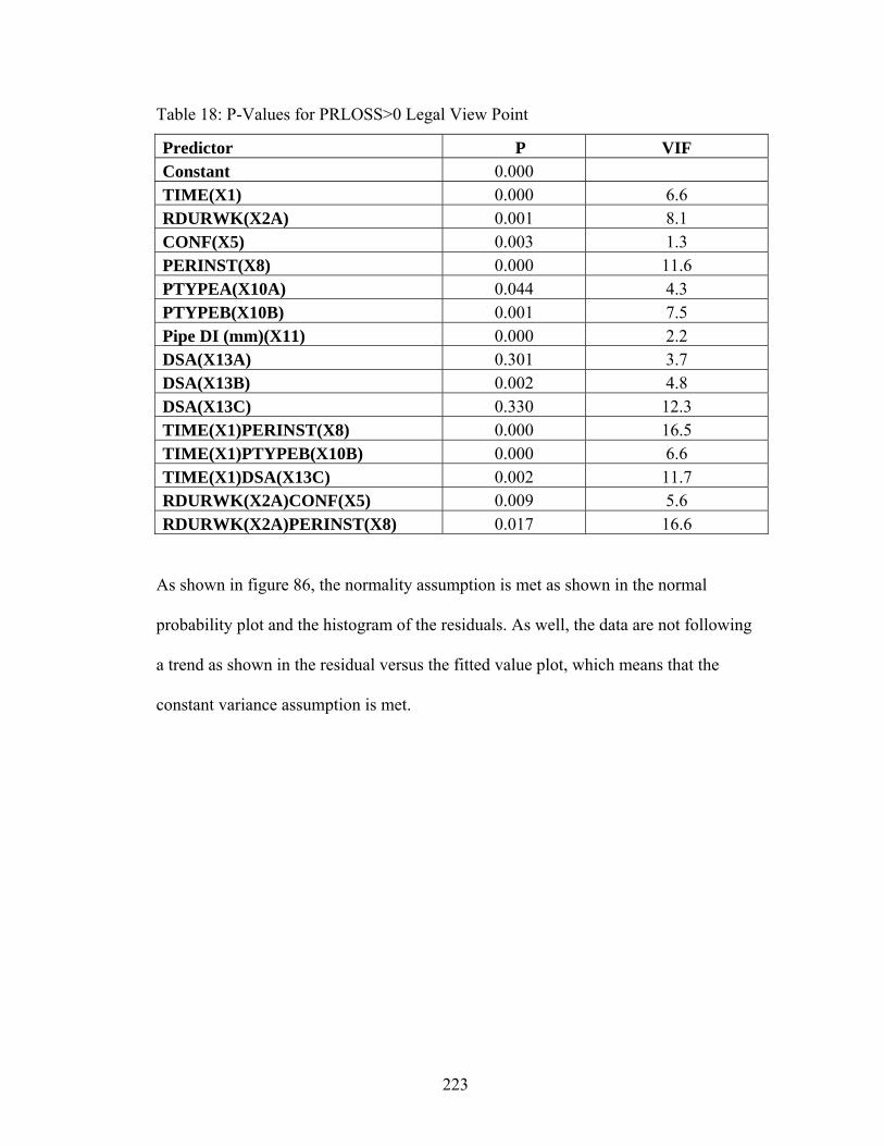
223

Table 18: P-Values for PRLOSS>0 Legal View Point

Predictor P VIF Constant 0.000 TIME(X1) 0.000 6.6 RDURWK(X2A) 0.001 8.1 CONF(X5) 0.003 1.3 PERINST(X8) 0.000 11.6 PTYPEA(X10A) 0.044 4.3 PTYPEB(X10B) 0.001 7.5 Pipe DI (mm)(X11) 0.000 2.2 DSA(X13A) 0.301 3.7 DSA(X13B) 0.002 4.8 DSA(X13C) 0.330 12.3 TIME(X1)PERINST(X8) 0.000 16.5 TIME(X1)PTYPEB(X10B) 0.000 6.6 TIME(X1)DSA(X13C) 0.002 11.7 RDURWK(X2A)CONF(X5) 0.009 5.6 RDURWK(X2A)PERINST(X8) 0.017 16.6

As shown in figure 86, the normality assumption is met as shown in the normal

probability plot and the histogram of the residuals. As well, the data are not following

a trend as shown in the residual versus the fitted value plot, which means that the

constant variance assumption is met.

224

Residual

Per

cent

0.500.250.00-0.25-0.50

99.9

99

90

50

10

1

0.1

N 88AD 0.321P-Value 0.526

Fitted Value

Res

idua

l

2.001.751.501.251.00

0.30

0.15

0.00

-0.15

-0.30

Residual

Freq

uenc

y

0.20.10.0-0.1-0.2-0.3

20

15

10

5

0

Observation Order

Res

idua

l

80706050403020101

0.30

0.15

0.00

-0.15

-0.30



Residual Plots for log PRLOSS

Figure 87: Residual Plot for PRLOSS>0% Legal View Point

4.4 Model Validation

A model should be evaluated to determine its robustness. Data from different projects

that were not used in the model building should be used in the model validation.

The following sections show the validation results for the change order models, both

for cumulative increase in the contract price due to change orders less and greater

than 5% and the piping model for productivity loss >0%, both from the owner and the

contractor view point.

225

4.4.1 Change Order Model PERCINC >5%

The validation data set consists of 29 observations from four projects that were not

used in the model building. The actual percent increase in the contract price due to

change order is compared to the predicted percent increase from the model. The

average percentage of error is 28.61% which is lower than 30.5%, 40.5%, and 53%

associated with the general regression model of Moselhi 1991, the electrical

regression model of Hanna 1999b, and the mechanical regression for Hanna 1999a.

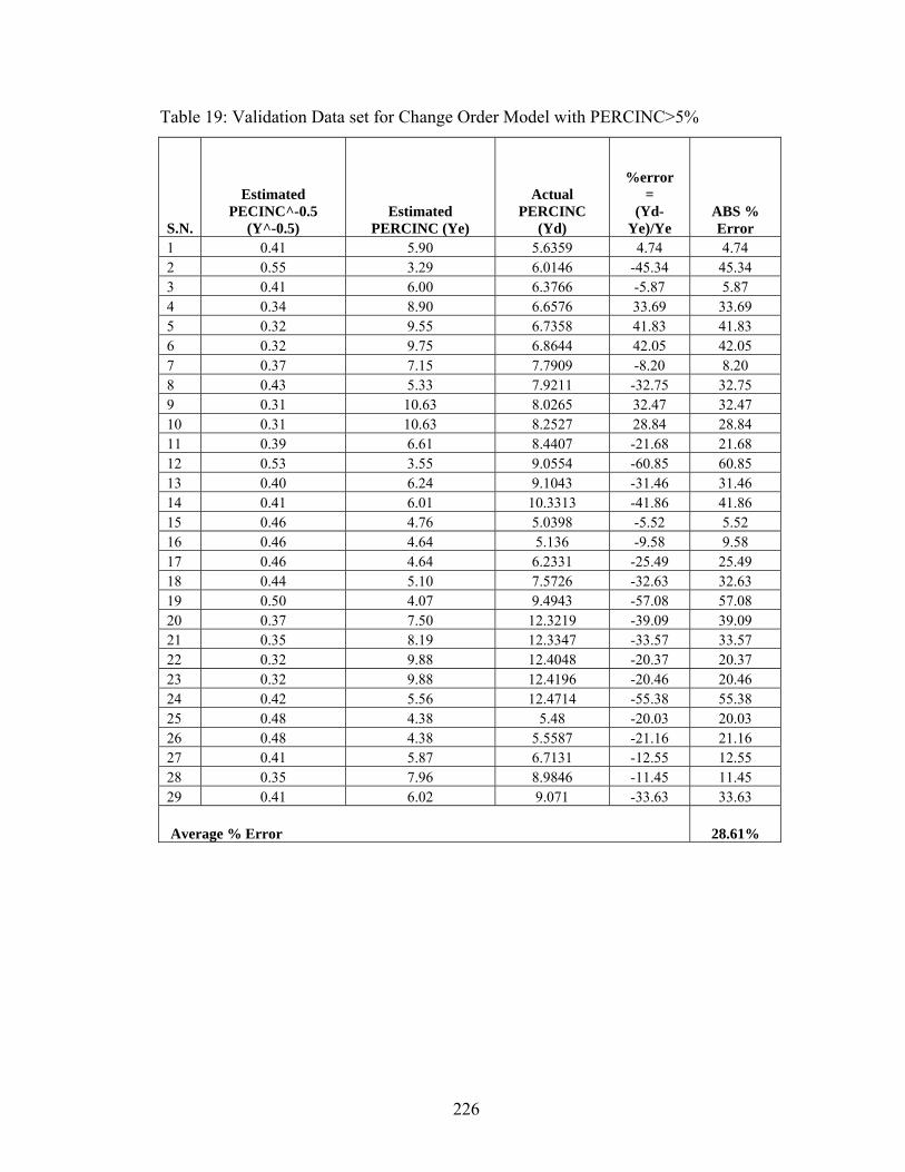
226

Table 19: Validation Data set for Change Order Model with PERCINC>5%

S.N.

Estimated PECINC^-0.5

(Y^-0.5) Estimated

PERCINC (Ye)

Actual PERCINC

(Yd)

%error =

(Yd-Ye)/Ye

ABS % Error

1 0.41 5.90 5.6359 4.74 4.74 2 0.55 3.29 6.0146 -45.34 45.34 3 0.41 6.00 6.3766 -5.87 5.87 4 0.34 8.90 6.6576 33.69 33.69 5 0.32 9.55 6.7358 41.83 41.83 6 0.32 9.75 6.8644 42.05 42.05 7 0.37 7.15 7.7909 -8.20 8.20 8 0.43 5.33 7.9211 -32.75 32.75 9 0.31 10.63 8.0265 32.47 32.47 10 0.31 10.63 8.2527 28.84 28.84 11 0.39 6.61 8.4407 -21.68 21.68 12 0.53 3.55 9.0554 -60.85 60.85 13 0.40 6.24 9.1043 -31.46 31.46 14 0.41 6.01 10.3313 -41.86 41.86 15 0.46 4.76 5.0398 -5.52 5.52 16 0.46 4.64 5.136 -9.58 9.58 17 0.46 4.64 6.2331 -25.49 25.49 18 0.44 5.10 7.5726 -32.63 32.63 19 0.50 4.07 9.4943 -57.08 57.08 20 0.37 7.50 12.3219 -39.09 39.09 21 0.35 8.19 12.3347 -33.57 33.57 22 0.32 9.88 12.4048 -20.37 20.37 23 0.32 9.88 12.4196 -20.46 20.46 24 0.42 5.56 12.4714 -55.38 55.38 25 0.48 4.38 5.48 -20.03 20.03 26 0.48 4.38 5.5587 -21.16 21.16 27 0.41 5.87 6.7131 -12.55 12.55 28 0.35 7.96 8.9846 -11.45 11.45 29 0.41 6.02 9.071 -33.63 33.63

Average % Error 28.61%

227

4.4.2 Change order Model PERCINC<5%


used in the model building. The actual percent increase in the contract price due to

change order is compared to the predicted percent increase from the model. The

average percentage of error is 43.94%, which is lower than 53% associated with the

mechanical regression for Hanna 1999a.

Table 20: Validation Data set for Change Order Model with PERCINC<5% S.N.

Estimated PECINC^0.4

(Y^0.4) Estimated

PERCINC (Ye)

Actual PERCINC

(Yd)

%error =

(Yd-Ye)/Ye ABS % Error

1 1.42 2.40 2.0927 14.74 14.74 2 1.41 2.37 2.0997 12.74 12.74 3 1.41 2.37 2.1388 10.68 10.68 4 0.89 0.75 2.1949 -65.98 65.98 5 1.40 2.32 2.9814 -22.10 22.10 6 1.45 2.55 3.1076 -18.03 18.03 7 1.51 2.81 3.4235 -17.82 17.82 8 1.10 1.26 0.8509 48.22 48.22 9 1.10 1.26 0.9936 26.93 26.93 10 0.83 0.63 1.1473 -45.52 45.52 11 1.41 2.38 1.2277 93.60 93.60 12 0.93 0.82 1.2986 -36.55 36.55 13 1.05 1.14 1.4748 -22.96 22.96 14 1.29 1.89 4.5508 -58.41 58.41 15 0.76 0.51 0.2848 77.99 77.99 16 0.61 0.30 0.3021 -2.33 2.33 17 0.52 0.19 0.3506 -45.35 45.35 18 0.62 0.30 0.7152 -58.13 58.13 19 0.77 0.52 0.8124 -36.50 36.50 20 0.57 0.24 2.2396 -89.11 89.11 21 0.80 0.58 3.3365 -82.60 82.60 22 0.77 0.52 3.3492 -84.47 84.47 23 0.77 0.52 4.2554 -87.70 87.70 24 1.11 1.31 0.8911 46.89 46.89 25 1.24 1.70 1.0838 56.55 56.55 26 1.12 1.33 1.3283 -0.14 0.14 27 1.26 1.77 1.4302 23.44 23.44 28 1.24 1.72 1.189 44.88 44.88 Average %Error 43.94%

228

4.4.3 Piping Model with PRLOSS >0% Suffered by the Contractor


used in the model building. The actual percent loss is compared to the predicted

percent loss from the model. The average % of error is 35%, which is lower than

40.5%, and 53% associated with the electrical regression model of Hanna 1999b, and

the mechanical regression for Hanna 1999a.

Table 21: Validation Data set for Piping Model with PRLOSS>0% Suffered by the Contractor

S.N.

Estimated PRLOSS^0.5

(Y^0.5) Estimated PRLOSS

(Ye)

Actual PRLOSS

(Yd)

%error =


1 8.74 76.37 150.00 -49.09 49.09 2 5.56 30.90 86.28 -64.19 64.19 3 -4.21 17.77 32.12 -44.70 44.70 4 -3.22 10.36 59.72 -82.65 82.65 5 13.02 169.57 400.00 -57.61 57.61 6 22.10 488.43 391.07 24.90 24.90 7 8.79 77.22 77.63 -0.53 0.53 8 10.51 110.47 127.37 -13.27 13.27 9 12.57 157.94 195.89 -19.37 19.37 10 5.48 30.07 41.67 -27.82 27.82 11 -1.90 3.62 4.74 -23.70 23.70 12 9.67 93.52 113.01 -17.24 17.24 13 5.45 29.73 19.12 55.48 55.48 14 6.92 47.93 123.79 -61.28 61.28 15 5.90 34.82 33.47 4.04 4.04 16 12.90 166.34 147.46 12.81 12.81 17 5.13 26.28 54.91 -52.14 52.14 18 2.94 8.67 6.61 31.21 31.21 19 4.41 19.44 25.00 -22.22 22.22 20 4.88 23.79 42.05 -43.42 43.42 21 3.31 10.95 14.04 -22.01 22.01 22 -2.36 5.56 4.88 13.94 13.94 23 3.39 11.49 15.27 -24.75 24.75 24 -3.34 11.13 20.46 -45.60 45.60 25 4.85 23.54 78.02 -69.82 69.82 26 -4.52 20.41 18.61 9.67 9.67 27 4.45 19.80 29.37 -32.58 32.58 28 5.29 28.00 60.49 -53.71 53.71 Average% Error 34.99%

229

4.4.4 Piping Model with PRLOSS >0% Legal View Point


used in the model building. The actual percent loss is compared to the predicted

percent loss from the model. The average % of error is 38%, which is lower than

40.5%, and 53% associated with the electrical regression model of Hanna 1999b, and

the mechanical regression model of Hanna 1999a.

Table 22: Validation Data set for Piping Model with PRLOSS>0% Legal View Point

S.N.

Estimated LOG PRLOSS (Log Y)

Estimated PRLOSS (Ye)

Actual PRLOSS (Yd)

%error =


1 1.32 21.02 41.67 -49.55 49.55 2 2.05 113.00 113.01 0.00 0.00 3 1.06 11.51 19.12 -39.78 39.78 4 1.62 41.74 123.79 -66.28 66.28 5 1.31 20.38 33.47 -39.09 39.09 6 1.65 44.45 54.91 -19.04 19.04 7 1.62 41.72 25.00 66.88 66.88 8 1.67 47.04 42.05 11.87 11.87 9 1.16 14.56 20.46 -28.83 28.83 10 1.81 64.72 78.02 -17.05 17.05 11 1.50 31.50 18.61 69.23 69.23 12 1.96 91.59 60.49 51.41 51.41 Average% Error 38%

230

4.5 Model Implementation

4.5.1 Introduction

To demonstrate how the change order model and the productivity loss model are

implemented, two case studies will be presented in this section (The name of the

contractor presented in the example does not represent a real contractor).

4.5.2 Loss of Productivity Case Study

Johnsons contracting company is a major contractor for Florida Department of

Transportation (FDOT). This contracting company is a General Contractor

specializing in heavy highway construction, site work and underground utilities.

Johnsons contracting was the lowest bidder for state project “XXXX-XXX”. The

scope of work included all the necessary demolition and clearing, installation of new

drainage structures, construction of new sanitary sewer and water lines and a

substantial amount of earthwork, re-grading, and paving to be done. The project

original duration is 605 days with the notice to proceed in August 22nd, 2002.

In June 1st, 2003 while the contractor was working on the storm drainage, a conflict

was encountered between structure 1 and structure 2. The contractor had to relocate

the piping to overcome this obstruction and asked the owner to issue a change order

to compensate them for the changed work. FDOT requested the contractor to prepare

a cost proposal for the changed work.

231

The contractor claimed there is a loss of productivity because of the conflict

encountered. The owner decided to investigate the problem to be able to determine

the actual loss encountered.

FDOT daily reports showed that the contractor had some dewatering problems during

the work from structure 1 to structure 2. Daily reports as well showed that while

excavation the piping crew encountered the telephone line and that they damaged the

line. The length of piping installed in between structure 1 and structure 2 is 80 m. The

total quantity of piping for the project is 4000 m. The pipe between structures 1 to

structure 2 is 900 mm RCP pipe.

The contractor started quantifying the productivity loss by filling the following table:

232

Table 23: Productivity Case Study Predictor Variables

Abbr. Variable Name

Variable Reference

Unit

Way of Calculation PR

LOSS

% P

rodu

ctiv

ity

Loss

Y % How much?

TIM

E

Tim

e

X1 %%77.46

605283

605)221(

==−

=indaysndAuguststJuneTime

RA

IN

Rai

n RDURX2A

RJUSTBX2B

0 0

C= No rain

DEW

P

Dew

ater

ing

Prob

lem

X3 1

Yes

MA

LAT/

NTS

P

Mat

eria

l Pr

oble

ms NTSPX4A

MLATX4B

0 0

C=No material problem

CO

NFL

ICT

Con

flict

En

coun

ter

ed X5 1 Yes

RW

K

Rew

ork X6 % 0%

CO

EQ/O

WEQ

/TH

PR

Acc

iden

t on

Site


1 0 0

Accident on site caused by the contractor’s resources

PER

INST

% Q

uant

ity

Inst

alle

d

X8 %%2100)

400080( =X

TRB

OX

Tren

ch

Box

X9 1 Yes

233

PTY

PE

Pipe

Ty

pe X10A

X10B

0 0

C=RCP

Pipe

D

I

Pipe

D

iam

eter

X11 mm

900

ASP

LN

Wor

k St

art X12 0

As Planned

DSA

Des

ign

Acc

urac

y

X13 X13B X13C X13D X13E

0 0 1 0 0

C. To provide for unforeseen work, grade changes, or alterations in the plans which couldn't reasonably have been contemplated in the original plans and specifications

LOC

Loca

tio

n

X14 1 Change in bid location

SE AS

ON

Sea

son X15 0 Same Season as planned during bid

According to the contractor, he used the values in table 23 to substitute in equation

29, which to quantify the productivity loss suffered by the contractor, to quantify the

loss of productivity encountered because of the conflict.

PRLOSS^0.5 =

9.54 - 0.102 TIME(X1) + 10.2 RDURWK(X2A) - 0.265 RJUSBRSTR(X2B)

+ 6.72 DEWP(X3) + 5.83 NTSP(X4A) + 0.356 CONF(X5) - 0.0855 RWK (X6)

+ 4.96 C0EQ(X7A) - 1.51 PERINST(X8) - 4.84 TRBX(X9)

+ 3.86 PTYPEA(X10A)

- 0.36 PTYPEB(X10B) - 0.00267 Pipe DI (mm)(X11) - 1.12 ASPLN(X12)

+ 3.29 DSA(X13A) - 1.96 DSA(X13B) + 0.20 DSA(X13C)

+ 0.0177 TIME(X1)PERINST(X8) - 0.0652 TIME(X1)PTYPEB(X10B)

+ 0.000053 TIME(X1)Pipe DI (mm)(X11) + 0.0434 TIME(X1)DSA(X13A)

+ 0.0586 TIME(X1)DSA(X13C) - 9.61 RDURWK(X2A)DSA(X13A)

- 3.55 DEWP(X3)PTYPEB(X10B) - 4.47 CONF(X5)C0EQ(X7A)

234

+ 0.639 CONF(X5)PERINST(X8) - 8.43 CONF(X5)DSA(X13C)

- 0.500 C0EQ(X7A)PERINST(X8) + 11.4 C0EQ(X7A)TRBX(X9)

- 8.70 TRBX(X9)PTYPEA(X10A)

+ 0.00386 PTYPEB(X10B)Pipe DI (mm)(X11)

- 0.00616 Pipe DI (mm)(X11)DSA(X13A)…………………………..……Eq. 29

By substituting in equation 29, PRLOSS= 141.5%.

The contractor best performance on site for the piping work is almost 4 man-

hour/Linear meter working in the following from one structure to another:

Trench excavation

Pipe bedding

Pipe laying

Backfilling & compaction

Thus he submits to the owner that his expected productivity after experiencing the

conflict is not 4 mh/m but equals to:

New Productivity due to loss= 4(1.45) + 4= 9.8mh/m

The contractor submit the cost proposal to the owner that as 9.88mh/m and multiplies

it by quantity from structure 1 to structure 2.

Man-hours expended from structure 1 to structure 2= 9.8 (mh/m) X 80m = 784 man-

hours

Less what the contractor should have without the conflict =4 (mh/m) X 80m = 320

man-hours

235

Therefore, the contractor asks the owner to compensate him for:

784-320= 464 man-hours for loss of productivity

The owner started reviewing the cost proposal; the owner will issue a change order

and compensate the contractor for the loss of productivity due to the changed work.

The owner started quantifying the loss and used the variables in table 22 and

substitute in equation 30, which is to quantify the productivity loss from the owner

view point where all the factors that are contributed by the contractor are eliminated.

Log PRLOSS =

2.35 - 0.00560 TIME(X1) + 0.785 RDURWK(X2A) + 0.182 CONF(X5)

- 0.251 PERINST(X8) + 0.348 PTYPEA(X10A) + 0.548 PTYPEB(X10B)

- 0.000694 Pipe DI (mm)(X11) - 0.0712 DSA(X13A) - 0.500 DSA(X13B)

- 0.169 DSA(X13C) + 0.00304 TIME(X1)PERINST(X8)

- 0.0189 TIME(X1)PTYPEB(X10B) + 0.00816 TIME(X1)DSA(X13C)

+ 0.894 RDURWK(X2A)CONF(X5)

-0.345 RDURWK(X2A)PERINST(X8)……………………….……..Eq. 30

By substituting in equation 30, PRLOSS= 43.82%.

The contractor best performance on site for the piping work is almost 4 man-

hour/Linear meter working in the following from one structure to another:

Trench excavation

Pipe bedding

Pipe laying

236

Backfilling & compaction

Thus he submits to the owner that his expected productivity after experiencing the

conflict is not 4 mh/m but equals to:

New Productivity due to loss= 4(0.43) + 4= 5.72 mh/m

Man-hours expended from structure 1 to structure 2 due to the conflict= 5.72 (mh/m)

X 80m = 457.6 man-hours

Less what the contractor should have without the conflict =4 (mh/m) X 80m = 320

man-hours

Therefore, the owner should compensate the contractor for loss productivity:

457.6mh-320mh= 137.6 man-hours

(vs. 464 man-hours requested by the contractor)

4.5.2.1 Loss of Productivity: Practical Application

Practically, the owner and the contractor can negotiate the difference between the

legal entitlement to the contractor versus the cumulative impact due to the change

order suffered by the contractor. This is an effort to reach a consensus of an amount

of entitlement to the loss of productivity due to change orders.

Reference to the previous example, the difference between the contractor and the

owner computation of productivity loss (470 man-hours -137.6 man-hours =332.4

237

man-hours) is the presence of dewatering problem, which is the responsibility of the

contractor, and the accident that took place due to the contractor’s resources.

The negotiation for the difference in the amount of entitlement can differ according to

the project nature, the schedule preparation and most important the amount of risk

that the contractor allocated for the project.

Each contract will have its own risk allocation plan between the parties that vary

between standard forms, clients and countries. The contractor should develop a

change order management plan to avoid the risks allocated with potential

mismanagement on site during change orders. In the change order management plan,

the contractor should discuss the risk of the productivity loss due to change orders

and any potential mismanagement on site during the change order periods. The use

of equation 29, “Productivity Loss Suffered by the Contractor”, will aid the contractor

to quantify the amount of potential risks caused by the contractor’s resources. This

will ease the negotiation between the owner and the contractor to reach a consensus

regarding entitlement.

4.5.3 Change Order Case Study

FDOT decided to extend the project limits in the north side of the road for state

project “XXXX-XXX. The project original duration is 605 days with the notice to

proceed in August 22nd, 2002.

238

FDOT aimed to have an estimate of expected cost of the change order to check if the

contingency amount will be enough, given that up to date, July 30th 2003, several

change orders have been issued and the cumulative percent increase in the contract

price due to change orders is 2.1%. The project original cost is $15million. It is not a

critical item and thus won’t extend the project completion date.

The owner filled table 24 below and substitute the values in equation 27, which is to

quantify the cumulative percent increase due to the change orders when cumulative

increase of the change orders to date are less than 5%.

239

Table 24: Change Order Case Study Predictor Variables Abb. Variable

Name

Variable Reference

Unit

Way of Calculation

PER

CIN

C

% In

crea

se

in c

ontra

ct

pric

e

Y % How much?

TIM

E

Tim

ing

of

Cha

nge

Ord

er

X1 %%53.56

605342

605)2230(

==−

=indaysndAugustJulyTime

REA

SON

Rea

son

for

Cha

nge

Ord

er

X2A X2B X2C X2D

0 0 1 0


PAR

TY

Party

Im

plem

entin

g C

hang

e

X3 1

Contractor

APP

CO

App

rove

d C

hang

e O

rder

H

ours

X4 % 0%

STO

P

Wor

k St

oppa

ge X5 0 No

RES

TAC

Res

trict

ed

Acc

ess X6 0 No

CO

EXP

Way

Cha

nge

Ord

er

Expe

nded

X7A X7B

1 0

Credit

240

CO

CM

P

Way

Cha

nge

Ord

er

Com

pens

ated

X8A X8B

1 0

Lump sum

EXT

Exte

nsio

n X9 % 0%

SEA

SON

Wor

k Se

ason

X10 1

Same season as bid

STK

TRA

D

Stac

king

of

Trad

es X11 0

No

PERCINC^0.4 =

1.56 + 0.00763 TIME(X1) + 0.365 REASON (X2A) + 0.139 REASON (X2B)


+ 0.00308 APPCO (X4) + 0.354 STOP(X5) - 0.947 COEXP(X7A)

- 0.912 COEXP(X7B) + 0.256 COCOMP(X8A) - 0.519 COCOMP(X8B)

+ 0.00832 EXT (X9) - 0.00699 TIME(X1)REASON (X2A)

- 0.00535 TIME(X1)REASON (X2C) - 0.00535 TIME(X1)REASON (X2D)

+ 0.112 REASON (X2A)APPCO (X4) - 0.480 REASON (X2A)STOP(X5)

- 0.385 REASON (X2B)PARTY(X3) - 0.342 REASON (X2B)STOP(X5)+

0.224 REASON (X2B)COCOMP(X8B) + 0.679 REASON

(X2C)COCOMP(X8A)

+ 0.850 REASON (X2C)COCOMP(X8B) - 0.263 PARTY(X3)STOP(X5)

+ 0.175 PARTY(X3)COEXP(X7A) - 0.401 PARTY(X3)COCOMP(X8B)

- 0.164 STOP(X5)COEXP(X7B) + 0.594 COEXP(X7A)COCOMP(X8B)

+ 0.759 COEXP(X7B)COCOMP(X8B)……………………………..……Eq. 27

241

By substituting in equation 27, the cumulative percent increase is 2.53%. Thus the percent increase due to this change order is 2.53-2.1=0.43%.

Therefore, the expected percent increase due to this change order will be:

0.43%X ($15M) = $64,500

242

CHAPTER 5: CONCLUSION

5.1 Introduction

This dissertation highlighted the problem of change orders in construction projects

and specifically in the heavy construction sector. In addition, the problem of

productivity loss and the effect of the change orders and other contractor-contributed

problem are analyzed. The dissertation is divided into two studies; the first part is the

change order study in heavy construction projects. This study involves studying the

change orders, and the reasons that contributed to the increase in the contract price

due to the change orders, develop and validate a mode to be used by the owner to

quantify the increase in the contract price due to change orders .A need for a model to

quantify the increase in the contract price due to the change order from the owner

verifiable date is essential as most of the studies in the quantification of the change

orders were based on contractors data, which results in disagreements regarding the

value of the change order and the development of claims between the owner and the

contractor. This model will be a tool that aids the owner in the forward or

retrospective pricing of the change orders impact at various phases of the project. The

second study involves analyzing the productivity of piping work in heavy

construction projects to develop and validate a model to quantify the productivity loss

of the piping work due to change orders. Piping activities were selected after

analyzing the change orders and where the researchers discovered several change

orders issued because of design errors and omissions, or conflicts in the piping work.

243

Most of the disagreements between the owner and the contractor is due to the

quantification method and amount of entitlement of productivity loss due to the

owner changes. Therefore, the need for a model that quantifies the productivity loss

of the piping work from the owner’s data; daily reports, log of changes, plans and

specifications is essential. This model will aid the owner to quantify the productivity

loss due to change orders, and to reduce the reliance on the use of the present models

that were based on productivity data supplied by the contractor, and which may be

biased against the owner.

5.2 Research Strength

The dissertation tackled the change orders and the loss pf productivity problems from

the owner’s verifiable data. The researchers conducted several interviews with a

public owner and claims consultants who work for parties, the owner and the

contractor. This research methodology distinguished it from similar studies conducted

in this area. The strength of the research includes:

− Data source: The database for both studies, the change order study and the

productivity study is based on the daily reports of the owner (usually used by

contractors when claims occur), the log of the change orders, drawings,

specifications and the claim documents.

− Base line Productivity: Most of the previous studies used the bid hours and

compared them to the actual earned hours to prove entitlement to productivity

244

loss. This is not a fair comparison as the contractor might unknowingly

disregard his mismanagement on the site or underestimation in the bid hours

to win the bid. The average best productivity achieved by the contractor is the

baseline productivity that the actual productivity is compared to; so as to

prove entitlement of the productivity loss due to the owner changes.

− The change order information is analyzed by the researchers from the log of

changes issued by the owner. For every project, each change order is recorded

together with the reason behind the change, the time of the change, the way

the change order is compensated (lump sum, unit price or time and material

basis), how the change order is expended (Credit, rework, or idle), which part

is performing the change (contractor/subcontractor), and the approved change

order hours. All of these factors will assist in accurate quantification of the

increase in the contract price due to change order and not only rely on

interviews and surveys filled by the contractors.

− The productivity loss model included the quantity in the model not just the

work-hours. Most of the previous studies just included the hours; either earned

or bid hours and did not take into account the quantity installed. From

analyzing productivity data of piping work as presented in Chapter four, the

productivity seems to improve with the increase in the quantity installed from

one structure to another; a phenomena which is explained by the learning

curve theory. Thus including the quantity installed not just the work hours will

245

provide an accurate representation when discussing productivity loss

problems.

− Avoided the use of questionnaires: The source of the data used to build a

statistical model to quantify the impact of the change orders and its effect on

the productivity loss has been a point of discussion recently. Some of the

studies did not mention origin of the data; one reason that discourages the

owner and the courts from accepting them as a method of damages

calculations. In this research the origin of the data is stated plus the number of

the data points used in each study. Also, not mentioning the number of the

data points used to build the statistical models to quantify the impact of the

change orders on the productivity discourages owners or consultants from

using them. In this study, the number of data points is stated for the change

order and productivity studies plus all the statistical information for each

model in terms of coefficient of determination R2 and the P-value for the

variables, variable of inflation (VIF), and the % error. These are variables that

owners and consultants want to see before attempting to use a study to prove

damage entitlement.

− Model Predictors: The choice of the predictors of the response variable in the

present models was based on survey results filled by contractors. The owner

perspective of the predictor variables, or in other words the factors that

contribute to the percent increase in the cost of the change order or the

246

productivity loss, was seldom mentioned. In addition, the predictor variables

were screened after that based on statistical significance tests. This research

developed a set of predictors for the change order model and the piping model

based on studying different claims of heavy construction projects and

specifically related to loss of productivity in the piping work and as well from

interviews with consultants that handled claims for both owners and

contractors.

− Statistical Method: Stepwise regression was used in most of the previous

empirical models developed in this area. Stepwise regression does not allow

the user input and the selection of the predictor is based entirely on the

statistical significance tests. In this study, the researchers performed backward

selection in the choice of the predictors. Though some of the variables were

statistically insignificant, the researchers kept them as they are significant

from the perspective of the experts interviewed.

− Contractor & Owner View Point: In the productivity study all the factors that

might contribute to the productivity loss caused by both the owner and the

contractor are included, then two models are developed; one that includes the

factors that both parties contribute to the increase in the productivity loss, and

another that include only the owner caused factors. The difference in the

entitlement amount, as shown in the case study in Chapter 4, explains the

247

reasons why the owners are reluctant to use the current models that are based

on data supplied by the contractor.

5.3 Major Findings

The research presented two studies, the first analyzed and quantified the percent

increase in the contract price due to change orders; and the second analyzed and

quantified the productivity loss of the piping work. The first step before building the

model was to visualize the data and observe trends between the response variable and

each of the predictors followed by the model formulation and validation. The

following section discusses the trends observed in each study.

5.3.1 Change Order Study

- The percent increase in the contract price in the contract price increases

with time. The percent increase jumps drastically after the planned

completion date of the project, which means that change orders issued

after the planned completion date is very expensive. This is due to the fact

that the contractor did not take such extension in consideration while

allocating his resources and charge the owner more money for the change

order.

- The most common reason for the owner issuing a change order is to

account for unforeseen conditions and alterations in the plan. A problem

248

that is very common in heavy construction projects as a lot of work is

done under the ground. This might be due poor design prepared by the

owner consultants or lack of a thorough study of the area before preparing

the design.

- Though issuing a change order for the deterioration or damage to the

project after design does not occur as frequently, it yielded the highest

percent increase in the contract price.

- Change orders performed by the subcontractor are more expensive than

those performed by the contractor. This is due to the fact that the

contractor adds overhead and profit to the subcontractor quote before

submitting to the owner.

- Work stoppage might not occur frequently due to the fact that the

contractor under the contract has to continue the work with his right to

submit a request for claim if he is not satisfied by the owner’s decisions.

- The highest percent increase in the contract price is when the change order

work is expended as idle work; where the owner compensate the

contractor for idle labor/ or equipment. The least percent increase in the

contract price when the change order is expended for credit work, either

249

addition or deletion, and this is due to the fact that the prices might be

agreed upon in the contract.

- The most expensive way of compensating the change order is as lump sum

followed by unit price and time and material basis (4.25%, 4.54%).

- Interaction of the variables is important to study the effect of the

increase/decrease of two independent variables together.

- Change orders less than 5% are almost common in most construction

projects. More than 5% is where quantification of the change order might

lead to disagreement between the owner and the contractor. The 5% limit

is supported by previous research by Adrian and Hanna; however there

was no reason listed behind this 5% limit.

- When the change order increases the contract price by more than 5%, the

most significant factors that explain the percent increase in the contract

price due to change orders are:

o Time

o Reason of the change (A,B&D)

o Party performing the changed work

o The way change order is compensated

o Extension

250

As for the interaction variables, the most significant interaction

variables that contribute to the increase in the contract price due to the

change order:

o Time and (reason of the change (A), approved change order

o restricted access, the way the change order is expended, and

how the change order is compensated)

o Reason (B) and (change order is expended as credit, change

order is compensated as time and material basis, extension is

granted)

o Reason (D) and (party, way the change order is expended,

when the change order is compensated as lump sum)

- When the change order increases the contract price by less than 5%, the

most significant factors that explain the percent increase in the contract

price due to change orders are:

o Time

o Reason for the change (A&D)

o Way the change order is expended

o How the change order is compensated


variables that contribute to the increase in the contract price due to the

change order are:

o Time and the reason of the change (A&D)

251

o Reason (A) and (approved change order hours)

o Reason (B) and (the party performing the change, and when the

change order is compensated as time and material basis)

o Reason (C) and the way the change order is compensated

o Party and the when the change order is compensated as time

and material basis

o The way the change order is expended and when the change

order is compensated as time and material basis

5.3.2 Loss of Productivity Study

- Productivity loss is high in the first 10% of the project as the labor is

mobilizing their equipment on site and getting adapted to the work type

and area. Also, Productivity loss is high in the last 10% of the project

during the punch list work item. Productivity loss increases dramatically

after the planned completion date for the project.

- Time is a very significant factor for the productivity loss, the later the

change order issued, the higher the productivity loss.

- Though the rainy days might be excusable non-compensable, productivity

loss is the highest when rain is encountered during the work from one

structure to another.

252

- Contractors have to plan their dewatering system adequately. If the

dewatering system is not adequately planned and installed in the site,

productivity loss will be encountered and the owner won’t be responsible

for such type of damage.

- When the contractor encounters conflicts/unforeseen conditions, this will

be entirely the responsibility of the owner, and the change order cost can

be very high.

- The quantity installed has a great impact on the productivity enhancement;

a phenomenon that is explained by the learning curve theory.

- When trench box is used, a requirement by the OSHA, the loss of

productivity is higher and this is due to the fact of the nature of installing

the trench box followed by the pipe laying operation.

- The pipe diameter is really a function of the pipe type. The smaller pipe

diameters are usually the sanitary sewer pipes. These pipes are usually

installed at the deepest level so as not to contaminate the potable water or

the storm water pipes. The deeper the excavation goes the higher the

probability of encountering conflicts, a factor that might explain the

highest loss of productivity in such type of pipes.

253

- CMP pipes tend to have the least productivity losses followed by RCP and

the highest is the PVC pipes which are mainly used for the sanitary sewer

pipes.

- Most of the change orders related to the piping work are due

conflicts/unforeseen conditions.

- When the materials purchased are not according to the projects

specifications the productivity loss is the highest followed by late material

delivery.

- Analyzing all the productivity loss suffered by the contractor, and

including all the factors that are attributed to both parties, the most

significant variables that contribute to the productivity loss are:

o Time

o Rain during work

o When dewatering problem is encountered

o When the materials are not according to the project specifications

o Rework

o When there is an accident caused by the contractor’s resources

o Quantity installed, and the use of trench box


variables that contribute to the productivity loss quantification are:

254

o Time and (percent installed, pipe type, time and pipe diameter

o when there is a change order issued for unforeseen conditions)

o When there is a dewatering problem and the pipe type

o When there is a conflict and (an accident on site due to the

contractor’s resources, the quantity installed)

o Accident on site and (quantity installed, and where trench box is

used)

o The use of trench box and the installation of PVC pipe

o Finally the use of CM and the pipe diameter

- When analyzing only the productivity loss factors that are attributed to the

owner, the most significant factors are:

o Time

o When rain is during work

o When there is a conflict encountered

o Quantity installed

o The pipe type and diameter


variables that contribute to the productivity loss quantification are:

o Time and the quantity installed

o Time and pipe type

o Time and when there is a change in design due to conflicts or

unforeseen conditions

255

o When there is a rain during work and a conflict encountered

5.4 Research Contributions

This is the first study to tackle the problem of loss of productivity and cost of the

change order from the owner verifiable data in heavy construction projects.

The change order model provided a tool to the owner to perform a forward or

retrospective pricing of change orders. It aids in forecasting the cash flow of the

owner and to make sure that the contingency money available for the project will

cover the cost of the change orders.

The productivity loss study analyzed all of the factors that contributed to the

productivity loss of the piping work and segregated the factors that are attributable to

the contractor. In this way both view points are presented, and both parties will be

able to quantify the damage encountered, where the contractor will learn from his

mistakes and develop a change order management system to handle the changes on

site, and the owner will be able to have an estimate of the productivity loss

encountered due the change orders.

The study avoided the bias of the existing models prepared from data supplied by the

contractor as the contractor might unknowingly disregard the loss of productivity

factors that can be in his control such as mismanagement in the site or

256

underestimation of the bid.

In the presence of the change order and the productivity loss models, where both

parties agree upon, the process of handling the changes and the quantification of the

damage will be easier and hence the owner’s and the contractor’s time and money

allocated for the dispute resolution will be minimized.

In addition, the research provided a tool to help the owners in heavy construction

projects, a trade that was seldom studied, to quantify the cost of the change orders at

different period of times during the lifetime of the project.

5.5 Future Work

The research analyzed piping work of heavy construction projects and a model was

developed to quantify the productivity loss of the piping work activities. Other trades

in heavy construction projects can be analyzed like clearing and grubbing, excavation

and milling and paving activities. This is very important as the type of the activities

will impact the predictors used to explain the response variable. This is one

disadvantage on the previous studies where one model is developed for the entire

sector of construction, for example electrical work, without breaking up into activities

and study each separately.

257

The study was based on heavy construction projects where design-bid-build is the

delivery method. Other delivery methods should be analyzed like the design-build

delivery method.

The number of predictors in the projects selected was eleven for the change order

study and fifteen for the piping work study. More variables should be studied to

check their impact on the percent increase of the change order cost and the

productivity loss.

Since the quantity installed seem to have a major impact on the productivity loss

model and its interaction with time. A model can be developed to estimate the

productivity improvement over time and include other variables such as the use of

trench box, pipe diameter and pipe material. This will be similar to the learning curve

theory and will be applicable to heavy construction projects in specific as most of the

learning curves are developed from the manufacturing industries.

The time, that the owner representative takes to review the request for information

(RFI) of the contractors on certain activities, and specifically for critical activities,

might have an impact on the increase on the contract price due to change orders. A

study should be developed to quantify the impact of the request for information time

and related factor on the percent increase in the contract price due to change orders.

258

The study was based on heavy construction projects constructed in Florida. The

impact of the predictor variables on the response, the percent increase in the change

order and the productivity loss might differ according to the weather and soil type.

Similar research procedures should be applied to other states to quantify the percent

increase in the change order and the productivity loss due to change orders.

259

APPENDIX A: MCAA FACTORS

260

Table A 1: MCAA Factors

Percent of Loss If

Condition Factor

Minor Average Severe

1. Stacking of Trades: Operations take place with physically limited

space. Results in congestions of personnel, inability to locate tools

conveniently, increased loss of tools, additional safety hazards.

Optimum crew sized cannot be utilized

10% 20% 30%

2. Morale and Attitude: excessive hazard, competition for overtime,

over-inspection, multiple contract changes and rework, disruption of

labor rhythm and scheduling, poor site conditions, etc..

5% 15% 39%

3. Reassignment of Manpower: loss occurs with move-on, move off

because of unexpected changes, excessive changes, or demand made to

expedite or reschedule completion of certain work phases. Preparation

not possible for orderly change

5% 10% 15%

4. Crew Size Inefficiency: additional men to existing crews “breaks up”

original team effort, affect labor rhythm. Applies to basic contract hours

also

10% 20% 30%

5. Concurrent Operations: stacking of the contractor’s own forces.

Effect of adding operation to already planned sequence of operations.

Unless gradual and controlled implementation of additional operations

made, factor will apply to all remaining and proposed contract hours

5% 15% 25%

6. Dilution of Supervision: Applies to both basic contract and proposed

change. Supervision must be diverted to a) analyze and plan change b)

stop and re-plan affected work c) take off, order and expedite material

and equipment. d) Incorporate changes into schedule. e) Instruct

foreman and journeyman f) supervise work in progress, and g) revise

10% 15% 25%

261

punch lists, testing and start up requirements.

7. Learning Curve: Period of Orientation in order to become familiar

with changed condition. If new men are added to projects, effects more

sever as they learn tool location, work procedures, etc. Turn over of

crew

5% 15% 30%

8. Errors and omissions: increase in errors and omissions because

changes usually performed on crash basis, out of sequence or cause

dilution of supervision or any other negative factor.

1% 3% 6%

9. Beneficial Occupancy: working over, around or in close proximity to

owner’s personnel or production equipment. Also, dust and special

safety requirements and access restriction because of owner. Using

premises by owner prior to contract completion.

15% 25% 40%

10. Joint Occupancy: change causes work to be performed while

facility occupied by other trades and not anticipated under original bid 5% 12% 20%

11. Site Access: Interference with convenient access to work areas, poor

man-lift management or large and congested worksites. 5% 12% 30%

12. Logistics: owner-furnished materials and problems of dealing his

storehouse people, no control over material flow of work areas. Also,

contract changes causing problems of procurement and delivery of

materials and re-handling of substituted materials at site

15% 25% 40%

13. Fatigue: unusual physical exertion. If on change order work and

men return to base contract work, effects also affect performance on

base contract.

8% 10% 12%

262

14. Ripple: changes in other trades’ work affecting our work such as

alteration of our schedule. A solution id to request at first job meeting

that all change notices/bulletins be sent to our Contract Manager

10% 15% 20%

15. Overtime: lower worker output and efficiency through physical

fatigue and poor mental attitude. 10% 15% 20%

16. Season and Weather Change: either very hot or very cold

10% 20% 30%

263

APPENDIX B: INDEPENDENT VARIABLES FOR TREE

MODEL, LEE 2004

264

Table A 2: Independent Variables for Tree Model, Lee 2004

Symbol How measured

Project 0=electrical 1=mechanical

Impact 0=unimpacted, 1=impacted

Indu 0=not, 1= industrial

New Land 0=not, 1= new land

Renov 0=not, 1= renovation

Comp 1=prime, 2=separate prime, 3=subcontractor

Operunit Percent operating Unit

OwnConc Owner concerned with 1=cost, 2=schedule, 3=both

PerChange Percent change (decimals)

PerDelta Percent delta

PerExtend Percent duration extended (decimal)

Team 0=not, 1=dedicated team

Owner 0=public, 1=private

Worktg Owner/contractor work together before, 0=no, 1=yes

OwnExp Owner experience with same type work, 0=no, 1=yes

PEAIPA Percent estimate/actualIpeak/average

PEAIA Percent estimate/actualIaverage

PEAIP Percent estimate/actualIpeak

PAIPA Percent actualIpeak/average

FED Fixed end date, 0=no, 1=yes

ExtReq Extension requested, 0=no, 1=yes

ExtGrant Extension granted, 0=no, 1=yes

PerDesPA Percent design completed prior to award

PerDesPC Percent design completed prior to construction

AECoord A/E coordinate design, 0=no, 1=yes

AESupport A/E support during construction, 0=no, 1=yes

NoDoc Number of design documents, 1–6

PerMater Percent material purchased by others

PerEquip Percent equipment purchased by others

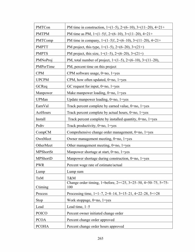
265

PMTCon PM time in construction, 1=(1–5), 2=(6–10), 3=(11–20), 4=21+

PMTPM PM time as PM, 1=(1–5)!, 2=(6–10), 3=(11–20), 4=21+

PMTComp PM time in company, 1=(1–5)!, 2=(6–10), 3=(11–20), 4=21+

PMPTT PM project, this type, 1=(1–5), 2=(6–20), 3=(21+)

PMPTS PM project, this size, 1=(1–5), 2=(6–20), 3=(21+)

PMNoProj PM, total number of project, 1=(1–5), 2=(6–10), 3=(11–20),

PMPerTime PM, percent time on this project

CPM CPM software usage, 0=no, 1=yes

UPCPM CPM, how often updated, 0=no, 1=yes

GCReq GC request for input, 0=no, 1=yes

Manpower Make manpower loading, 0=no, 1=yes

UPMan Update manpower loading, 0=no, 1=yes

EarnVal Track percent complete by earned value, 0=no, 1=yes

ActHours Track percent complete by actual hours, 0=no, 1=yes

Install Track percent complete by installed quantity, 0=no, 1=yes

Prdtv Track productivity, 0=no, 1=yes

CompCM Comprehensive change order management, 0=no, 1=yes

OwnMeet Owner management meeting, 0=no, 1=yes

OtherMeet Other management meeting, 0=no, 1=yes

MPShortSt Manpower shortage at start, 0=no, 1=yes

MPShortD Manpower shortage during construction, 0=no, 1=yes

PWR Percent wage rate of estimate/actual

Lump Lump sum

TnM T&M

Ctiming Change order timing, 1=before, 2=<25, 3=25–50, 4=50–75, 5=75-100

Process Processing time, 1=1–7, 2=8–14, 3=15–21, 4=22–28, 5=>28

Stop Work stoppage, 0=no, 1=yes

Lead Lead time, 1–5

POICO Percent owner initiated change order

PCOA Percent change order approved

PCOHA Percent change order hours approved

266

PerAdd Percent addition or deletion

PerDesign Percent design

Absentee Absenteeism, 1–4

Turnover Turnover, 1-4

PerOvert Percent overtime

overtime overtime, 0=no, 1=yes

Shiftwork Shift work, 0=no, 1=yes

Overman Overmanning, 0=no, 1=yes

267

APPENDIX C: A SAMPLE OF THE INPUT DATA

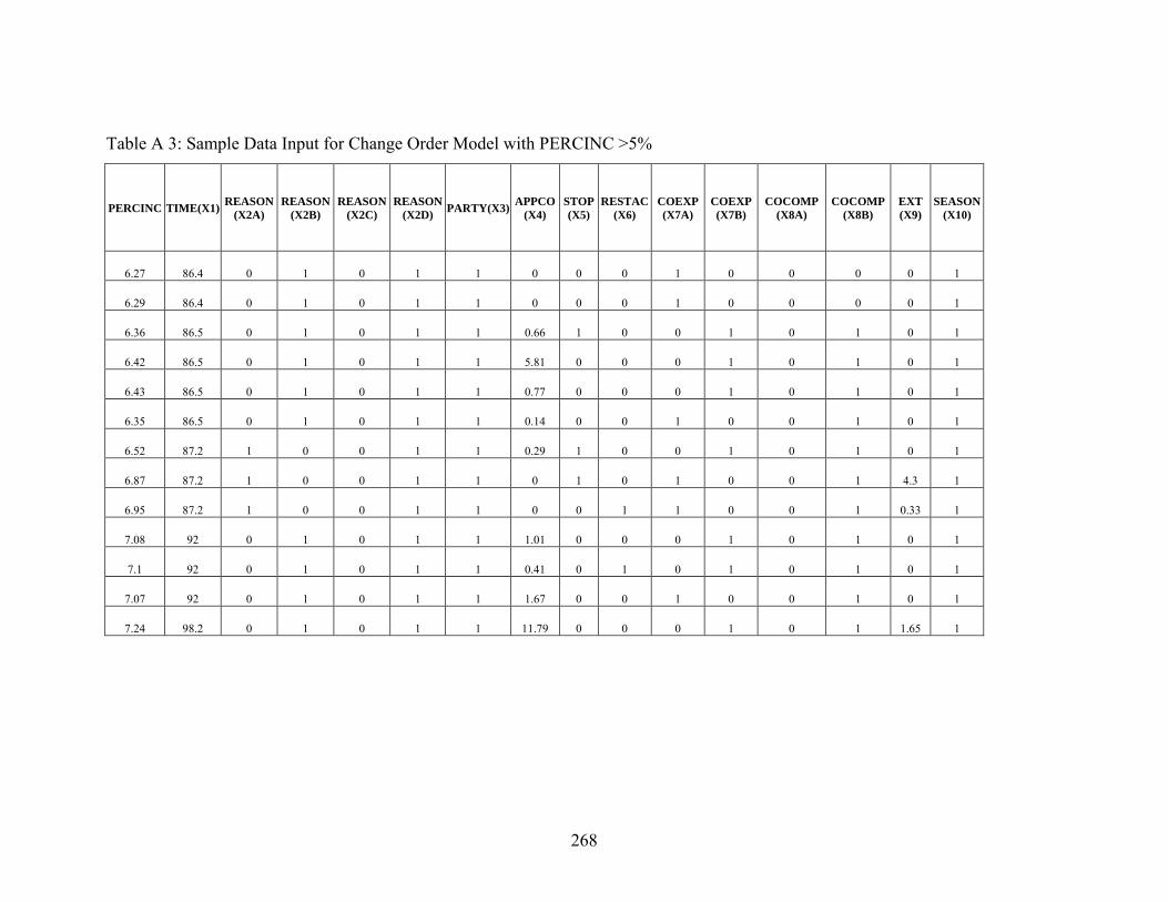
268

Table A 3: Sample Data Input for Change Order Model with PERCINC >5%

PERCINC TIME(X1) REASON (X2A)

REASON (X2B)

REASON (X2C)

REASON (X2D) PARTY(X3) APPCO

(X4) STOP(X5)

RESTAC(X6)

COEXP (X7A)

COEXP(X7B)

COCOMP (X8A)

COCOMP(X8B)

EXT (X9)

SEASON(X10)

6.27 86.4 0 1 0 1 1 0 0 0 1 0 0 0 0 1

6.29 86.4 0 1 0 1 1 0 0 0 1 0 0 0 0 1

6.36 86.5 0 1 0 1 1 0.66 1 0 0 1 0 1 0 1

6.42 86.5 0 1 0 1 1 5.81 0 0 0 1 0 1 0 1

6.43 86.5 0 1 0 1 1 0.77 0 0 0 1 0 1 0 1

6.35 86.5 0 1 0 1 1 0.14 0 0 1 0 0 1 0 1

6.52 87.2 1 0 0 1 1 0.29 1 0 0 1 0 1 0 1

6.87 87.2 1 0 0 1 1 0 1 0 1 0 0 1 4.3 1

6.95 87.2 1 0 0 1 1 0 0 1 1 0 0 1 0.33 1

7.08 92 0 1 0 1 1 1.01 0 0 0 1 0 1 0 1

7.1 92 0 1 0 1 1 0.41 0 1 0 1 0 1 0 1

7.07 92 0 1 0 1 1 1.67 0 0 1 0 0 1 0 1

7.24 98.2 0 1 0 1 1 11.79 0 0 0 1 0 1 1.65 1

269

Table A 4: Sample Data Input for Change Order Model with PERCINC <5%

PERCINC TIME(X1) REASON (X2A)

REASON (X2B)

REASON (X2C)

REASON (X2D) PARTY(X3) APPCO

(X4) STOP(X5)

RESTAC(X6)

COEXP (X7A)

COEXP(X7B)

COCOMP (X8A)

COCOMP(X8B)

EXT (X9)

SEASON(X10)

2.76 33.43 0 1 0 0 1 0 0 0 1 0 1 0 23.14 1

2.78 34.4 0 0 0 1 0 0.57 0 0 1 0 0 1 0 1

3.03 44.61 1 0 0 0 1 0 0 0 0 1 1 0 0 1

3.13 44.61 0 1 0 0 0 0 0 0 1 0 0 1 0 1

2.76 46.45 0 0 0 0 0 0 0 0 0 1 1 0 0 1

3.72 54.62 1 0 0 0 1 0 0 0 1 0 1 0 7.44 1

4.06 55.1 0 0 0 1 1 0 0 0 1 0 1 0 0 1

2.77 62.29 0 1 0 0 1 0.16 0 0 1 0 0 1 0 1

2.11 87.692 0 1 0 0 1 0 0 0 1 0 0 0 0.84 1

2.17 89.231 0 1 0 0 1 8.12 0 0 0 1 0 1 0 1

2.76 33.43 0 1 0 0 1 0 0 0 1 0 1 0 23.14 1

2.78 34.4 0 0 0 1 0 0.57 0 0 1 0 0 1 0 1

3.03 44.61 1 0 0 0 1 0 0 0 0 1 1 0 0 1

270

Table A 5: Sample Data Input for Piping Model with PRLOSS>0% Suffered by the Contractor

PRLOSS TIME (X1)

RDURWK (X2A)

RJUSBRSTR (X2B)

DEWP(X3)

NTSP (X4A)

MATLT(X4B)

CONF(X5)

RWK (X6)

C0EQ(X7A)

PERINST (X8)

TRBX(X9)

PTYPEA (X10A)

PTYPEB(X10B)

Pipe DI (mm)(X11)

ASPLN(X12)

DSA (X13A)

DSA (X13B)

DSA (X13C)

LOC (X14)

10.39 61.8 0 0 0 0 0 0 0 0 0.8337 0 0 1 1050 0 1 0 0 0

46.093 66.7 0 0 0 0 0 0 0 1 1.0645 0 0 1 1200 0 1 0 0 0

3.214 67.8 0 0 0 0 0 0 0 0 0.4318 0 0 1 1200 0 1 0 0 0

0.215 71.6 0 0 0 0 0 1 0 0 0.9454 0 0 1 1050 0 0 1 0 1

7.498 37.5 0 0 0 0 0 0 0 0 0.8114 0 0 0 900 0 1 0 0 0

19.836 38.5 0 0 0 0 0 0 0 0 0.6551 0 0 0 900 0 1 0 0 0

36.702 47.6 0 0 0 0 0 0 0 0 0.3573 0 0 0 750 0 1 0 0 0

71.99 32.7 0 0 0 0 0 0 0 0 0.1638 0 0 0 450 0 1 0 0 0

14.626 34.4 0 0 0 0 0 0 0 0 0.5211 0 0 0 600 0 0 1 0 0

271

Table A 6: Sample Data Input for Piping Model PRLOSS>0% Legal View Point

PRLOSS TIME (X1)

RDURWK (X2A)

RJUSBRSTR (X2B)

CONF(X5)

PERINST (X8)

TRBX (X9)

PTYPEA(X10A)

PTYPEB(X10B)

Pipe DI (mm)(X11)

ASPLN (X12)

DSA (X13A)

DSA (X13B)

DSA (X13C)

LOC (X14)

74.353 21.65 0 0 1 1.4026 0 1 0 254 0 0 1 0 0

40.265 22.31 0 0 0 2.3471 0 1 0 203 0 0 1 0 0

28.603 22.81 0 0 0 1.7789 0 1 0 203 0 0 1 0 0

20.048 23.64 0 0 0 0.5062 0 0 1 1200 0 1 0 0 0

28.458 24.48 0 0 0 0.6848 0 0 1 1050 0 1 0 0 0

71.99 32.73 0 0 0 0.1638 0 0 0 450 0 1 0 0 0

11.065 37.34 0 0 0 0.3648 0 0 1 1200 0 1 0 0 0

19.836 38.46 0 0 0 0.6551 0 0 0 900 0 1 0 0 0

9.091 44.62 0 0 0 0.4466 0 0 1 1050 0 1 0 0 0

36.702 47.55 0 0 0 0.3573 0 0 0 750 0 1 0 0 0

272

LIST OF REFERNCES

1. Adrian, James “Construction Productivity Improvement” Elsevier Science

Publishing Co. Inc., USA, 1987.

2. Appeal of Clark Construction Group, Inc. (2000 WL 37542) VABCA No. 5674,

00-1 BCA 30,870 ( Clark), 2000.

3. A J Mccormack & Son, “Drainage Installation”

http://www.pavingexpert.com/drain02.htm, Accessed May, 2006.

4. Coffman, G. “Effect of change orders on labor productivity.” 5th Construction

Congress V, ASCE, Reston, Va., 141–148, 1997.

5. Amelco V. City of Thousand Oaks (California Supreme Court No. S091069, filed

2/4/2002.

6. American Association of Cost Engineers AACE Education Board. “Practical

project control.” 33rd Annual Meeting, AACE, Skills and Knowledge of Cost

Engineers, Section 4.6, San Diego, 1989.

7. Bent, J., and Thuman, A. “Project Management for Engineering and

Construction.” Prentice–Hall, Englewood Cliffs, N.J, 1988.

8. Branton, Regina: Department of Political Science, Rice University

http://www.ruf.rice.edu/~branton/interaction/faqfund.htm, Accessed May, 2006.

9. Bruggink, M “An Investigation Into the Impacts of Change Orders on Labor

Efficiency in the Electrical Construction Industry.” Mac thesis, Univ. of

Wisconsin-Madison, Wisc., 1997.

10. Brunies, Regula and Emir, Zey “Calculating Loss of Productivity Due to

Overtime Using Published Charts-Facts or Fiction”. Revay Associated Limited,

273

Volume 20, No.3, November 2001.

11. Chick, David “The Time Value of Project Change” Journal of Cost Engineering,

Vol.41/No.6, June 1999.

12. Crowley, D., and Livengood, J.C. “Measured mile analysis and international

mega-projects.” AACE International, Transactions of the Annual Meeting, 2002.

13. Derksen, S. and H. J. Keselman.. “Backward, forward and stepwise automated

subset selection algorithms: frequency of obtaining authentic and noise variables”.

British Journal of Mathematical and Statistical Psychology , 1996, 45: 265–282.

14. Eden, Colin, Williams, Terry, and Franck Ackermann “Issues with the Measured

Mile” European Academy of Management (EURAM), 2003.

15. Elte, Inc. S.S. Mullen, Inc. (9th Cir. 1972) 469 F.2d 1127, 1972.

16. Emir, Zey. “Learning Curve in Construction” Revay and Associated Limited.

Volume 18, No.3, October 1999.

17. Farbaric, John J. “Discussion of ‘‘Impact of Change Orders on Labor Efficiency

for Electrical Construction’’ Journal of Construction Engineering and

Management, ASCE 2002. 362-363.

18. Finke, Michael “A Better Way to Estimate and Mitigate Disruption” Journal of

Construction Engineering and Management, November 1998b, 490-497.

19. Finke, Michael Rose “Statistical evaluation of Measured Mile Productivity

Claims”. Journal of Cost Engineering, Vol.40/N0.12, December 1998a.

20. Florida Department of Transportation “Standard Specifications for Road and

Bridge Construction”, Tallahassee, Florida, 2004.

21. Foulger, Davis Presented at the 1979 Annual Conference of the Speech

274

Communication Association, San Antonio, TX, 1979.

22. Gulezian, Ronald, and Samelian, Fredric “Baseline Determination in Construction

Labor Productivity-Loss Claims” Journal of Management in Engineering, ASCE,

October 2003, 160-165.

23. Habing, Brian “Transformation of Variables”. University of South Carolina, July

11, 2004.

24. Hanna, Awad S, Russell , Jeffrey S., Gotzion, Timothy W., and Erik V.

Nordheim “Impact Of Change Orders on Labor Efficiency for Mechanical

Construction” Journal of Construction Engineering and Management, ASCE,

1999a, 176-184.

25. Hanna, Awad S., Russell, J. S., Nordheim, E. V., and Bruggink, M. J. ‘‘Impact of

Change Orders on Labor Efficiency for Electrical Construction.’’ Journal of

Construction Engineering and Management”, ASCE, 1999b, 224–232.

26. Hanna, Awad S.; Camlic, Richard, Peterson, Pehr A., and Erik V. Nordheim

“Quantitative Definition of Projects Impacted by Change Orders”, Journal of

Construction Engineering and Management, ASCE, 2002.

27. Hanna, Awad S., and Sulllivan, Kenneth T. “Factors Affecting Labor Productivity

for Electrical Contractors” The Electrical Contracting Foundation, Betheda, MD,

2004.

28. Hanlon D&S Co. v. S.Pac. Co. 92 Cal.App. 230, 235, 1928.

29. Ibbs, C. “Quantitative impacts of project change: Size issues.” Journal of

Construction Engineering and Management, 1997, 308–311.

30. Ibbs, C. W., and Allen, W. E. ‘‘Quantitative Impacts of Project Change.’’ Source

275

Document 108, Construction Industry Institute, University of Texas at Austin,

Austin, Tex., 1995.

31. Lee, Min-Jae, Hanna, Awad S. and Wei-Yin Loh “Decision Tree Approach to

Classify and Quantify Cumulative Impact of Change Orders on Productivity”

Journal of Computing In Civil Engineering, ASCE, 2004, 132-144.

32. Leonard, Charles A. “The Effects of Change Order on Productivity”. Masters

Thesis, Concordia University, Canada, April, 1987.

33. Loulakis, Michael C. and Simon J. Santiago “Getting The Most out of Your

Measured Mile Approach , Journal of Civil Engineering, ASCE November,

1999, Vol. 69, Issue 11.

34. Loulakis, Michael C.; Gaba, Carmody; Rodrigues, Jared “The Law” Journal of

Civil Engineering, ASCE November 2003, Vol. 73 Issue 11.

35. Meyers, J. “Changes Resulting From delays” Construction Change order Claims.

John Wiley and Sons, Inc., Somerset, N.J., 1994.

36. Mechanical Contractors Association of America. Change Orders / Overtime /

Productivity. Rockville, Maryland, 1994.

37. National Electrical Contractors Association. Guide to Electrical Contractor’s

Claims Management Vol. I. Bethesda, Maryland, 2000.

38. Moselhi, O. ‘‘Estimating the cost of change orders.’’ AACE Int. Transactions,

Association for the Advancement of Cost Engineering, International,

Morgantown, W.Va, 1998.

39. Moselhi, O., Charles, L., and Fazio, P “Impact of Change Orders on construction

Productivity.” Canadian Journal of Civil Engineering, 1991, 484–492.

276

40. Moselhi, Osama, Assem, Ihab and Khaled El-Rayes “Change Orders Impact on

Labor Productivity” Journal of Construction Engineering and Management,

March 2005.

41. National Electrical Contractors Association NECA “Rate of Manpower

Consumption in Electrical Construction.” NECA, Washington, D.C., 1983.

42. National Electrical Contractors Association, Bethesda, MD. Overtime and

Productivity In Construction. 1969.

43. National Electrical Contractors Association, Bethesda, MD. Overtime and

Productivity in Electrical Construction, 2nd edition, 1989.

44. National Electrical Contractors Association, Washington, D.C. Overtime Work

Efficiency Survey, 1962.

45. Osman III, Goerge “Discussion of “Quantitative Definition of Projects Impacted

by Change Orders” Journal of Construction Engineering and Management,

ASCE 2004. 611-614.

46. Pinnel, Steven S. “How to get Paid for Construction Changes” McGraw-Hill

Companies Inc., USA, 1998.

47. Presnell, Thomas W. “Measured Mile Process” Cost Engineering Journal,

Vol.45/No.11 November 2003, 14-20.

48. Ringwald, Richard C. “Means Heavy Construction Handbook” R.S. Means

Company Inc., Kingston, MA, 1993.

49. Robinson, Aminah, Dissanayake, Manjula, and Oswaldo Campero, M.”

Measuring and Classifying Construction Field Rework: A Pilot Study”. Presented

to Construction Owners Association of Alberta (COAA), Field Rework

277

Committee, May 2003.

50. Shwartzkoph, William” Calculating Lost labor Productivity in Construction

Claims” John Wiley &Sons Inc., Canada, 1995.

51. Shwartzkoph, W., J. McNamara, and J. Hoffar “Calculating Construction

Damages”. John Wiley &Sons, USA, 1992.

52. Singh, R. “CPM as a tool in claims management.” AACE International.

Transactions of the Annual Meeting, CDR141-CDR142, 2002.

53. Stat soft, Inc., “General Regression Models”

http://www.statsoft.com/textbook/stgrm.html, Accessed December 2005.

54. Stumph, George. “Schedule Delay Analysis”. Journal of Cost Engineering,

Vol.42/No.7, July 2000.

55. Thomas, H. and Napolitan, C. “The Effects of Changes on Labor Productivity:

Why and How much”. Construction Industry Institute, University of Texas,

Austin, 1995a.

56. Thomas, H. Randoplh and Napolitan, Carmen L. “Quantitative Effects of

Construction Changes on Labor Productivity” Journal of Construction

Engineering and Management, ASCE 1995b, 290-296.

57. Thomas, H. Randoplh and Sanvido, Victor E. “Quantification of Losses Caused

by Labor inefficiencies: Where is the Elusive Measured Mile?” Journal of

Construction Law and Business, Vol. 1(3):1-14, Aspen Law and Business, New

York, 2000.

58. Thomas, H. Randoplh and Zavrski, Ivica “Construction Baseline Productivity:

Theory and Practice” Journal of Construction Engineering and Management,

278

ASCE 1999, 295-303.

59. Thomas, H.R., and Oloufa, A. “Strategies for minimizing the economic

consequences of schedule acceleration and compression” The Electrical

Contracting Foundation, Betheda, MD, 1996.

60. Thomas, H.R., and Oloufa, A. “Negotiating Loss of Labor Efficiency for

Electrical Contractors”. The Electrical Contracting Foundation, Betheda, MD,

2001.

61. Thomas, Randolph H., Raynar, Karl A. “Scheduled Overtime and Labor

Productivity: Quantitative Analysis” Journal of Construction Engineering and

Management, ASCE, June 1997, 181-188.

62. US Army Corps of Engineers, “Construction Modification Impact Evaluation

Guide”, 1979.

63. Vandenberg, P. “The Impact of Change Orders on Mechanical Construction

Labor Efficiency.” MSc thesis, Univ. of Wisconsin Madison, Wisc., 1996.

64. Warwick Construction Inc. GSBCA Nos. 5070 et al., 82-2 BCA 16,091 at 79,854.

65. Wideman, Max “"A Pragmatic Approach to Using Resource Loading, Production

and Learning Curves on Construction Projects” Canadian Journal of Civil

Engineering, Vol. 21, 1994 pp 939-953.

66. Wunderlich Contracting Co. v. United States, 173 Ct. Cl. 180, 1966.

CHANGE ORDERS AND PRODUCTIVITY LOSS QUANTIFICATION

Documents

Transcript of CHANGE ORDERS AND PRODUCTIVITY LOSS QUANTIFICATION