Copyright by Nuntapong Ovararin 2001 · The Dissertation Committee for Nuntapong Ovararin ......
258
Copyright by Nuntapong Ovararin 2001
Transcript of Copyright by Nuntapong Ovararin 2001 · The Dissertation Committee for Nuntapong Ovararin ......

Copyright
by
Nuntapong Ovararin
2001

The Dissertation Committee for Nuntapong Ovararin
Certifies that this is the approved version of the following dissertation:
QUANTIFYING PRODUCTIVITY LOSS DUE TO FIELD DISRUPTIONS
IN MASONRY CONSTRUCTION
Committee:
_________________________________ Calin M. Popescu, Supervisor
_________________________________ John D. Borcherding
_________________________________ G. Edward Gibson, Jr. _________________________________
Stephen R. Thomas
_________________________________ Daniel A. Powers

QUANTIFYING PRODUCTIVITY LOSS DUE TO FIELD DISRUPTIONS
IN MASONRY CONSTRUCTION
by
Nuntapong Ovararin, B.Eng., M.S.
Dissertation
Presented to the Faculty of the Graduate School of
The University of Texas at Austin
in Partial Fulfillment
of the Requirements
for the Degree of
Doctor of Philosophy
The University of Texas at Austin
December, 2001

UMI Number: 3040635
________________________________________________________
UMI Microform 3040635
Copyright 2001 by ProQuest Information and Learning Company.
All rights reserved. This microform edition is protected against
unauthorized copying under Title 17, United States Code.
____________________________________________________________
ProQuest Information and Learning Company300 North Zeeb Road
PO Box 1346Ann Arbor, MI 48106-1346

To my parents and my brothers and sisters
for their love, support, and encouragement.

ACKNOWLEDGEMENTS
I would like to express my appreciation to the members of my advisory
committee for their direction and guidance. My special thanks are extended to my
supervising professor, Dr. Calin M. Popescu, who has been extremely helpful and
supportive throughout the study. I am very grateful for his advice and personal
concern for the study. His encouragement and the confidence he placed in me during
the study made the task a lot more enjoyable. I would also like to thank Dr. John D.
Borcherding for his guidance in developing the questionnaires and supervising the
subject matter. His willingness to share his time and profound insight into the subject
matter contributed to making this study a positive learning experience.
I am grateful to Dr. G. Edward Gibson, Jr., for his support and assistance in
this research effort. His helpful discussions and comments on the study are gratefully
acknowledged. I would also like to thank Dr. Stephen R. Thomas for his time and
guidance in the research survey. His expertise and understanding of research surveys
made working with him a genuine delight. Additionally, I wish to acknowledge Dr.
Daniel A. Powers for his guidance in supervising the statistical analysis procedures.
His valuable time and helpful comments are greatly appreciated.
Special thanks also go to Mr. Jeff Buczkiewicz, Director of Marketing for
Mason Contractors Association of America, who distributed and collected the
questionnaires, which played an important role in the success of the study.
Appreciation is also extended to Mr. Jim Crook and Mr. Chuck Pollard, Resident
Construction Managers of the Office of Facilities Planning and Construction at the
University of Texas at Austin, for their support and assistance in facilitating the
model validation process. Without their support, this research could not have been
successfully accomplished.
v

I would also like to thank Mr. Kan Phaobunjong, Ms. Eunhee Kim, Mr. Unsuk
Jung, Mr. Hyoungkwan Kim, Mr. Yu-Ren Wang, and other friends in the CEPM
program, who were willing to take a little time to listen whenever I had anything to
say. Further thanks go out to Dr. Thanachan Mahawanuch and Ms. Tattaya
Hanbenjapong for their caring support and encouragement. Finally, I owe my deepest
gratitude to my parents and my brothers and sisters for their never-ending love and
encouragement throughout my graduate studies. Without their continued support and
concern, I would never have succeeded in such an encompassing endeavor.
vi

QUANTIFYING PRODUCTIVITY LOSS DUE TO FIELD DISRUPTIONS
IN MASONRY CONSTRUCTION
Publication No. ______________
Nuntapong Ovararin, Ph.D.
The University of Texas at Austin, 2001
Supervisor: Calin M. Popescu
Many research studies have proven that productivity loss is the result of
several factors including excessive change orders, long periods of overtime, poor
field management and severe weather. These factors generate further disruptions
affecting masonry productivity, and result in productivity loss or additional work-
hours to be required to perform masonry work. Unfortunately, estimators have had
difficulties in quantifying this productivity loss because no data of normal
productivity without an impact of field factors is available for determination of such
loss. The quantitative evaluation of productivity loss due to field disruptions in
masonry construction is therefore needed.
This research study presents a quantitative evaluation of productivity loss due
to field disruptions, based on a national survey. This study is intended to be a
reference tool for masonry practitioners in construction claims, construction
estimating, planning and scheduling. The primary objective of this study was to
quantify productivity loss caused by sixteen different field disruptions based on three
levels of standard field conditions for masonry building construction. With respect to
vii

this objective, a model used to estimate productivity loss or additional work-hours
due to the impact of field disruptions was developed, based on a national survey
conducted in the year 2000. A total of 950 questionnaires were randomly distributed
to masonry contractors throughout the U.S., and 152 questionnaires were collected.
The model presents an averaged percentage of productivity loss due to field
disruptions, along with a range of possible loss that may exist. Masonry practitioners
can employ the results of this survey to determine additional work-hours needed to
perform the masonry work in field conditions that differ from original expectations.
Through a second research survey, conducted in Texas, the model was tested
using five masonry construction projects facing field disruptions. It was found that
the differences in the estimated and actual percentages of productivity loss ranged
from -2 to 19%. In this dissertation, research procedures, conclusions, and
recommendations for industry and future research are also discussed.
viii

TABLE OF CONTENTS
ACKNOWLEDGEMENTS ……………………………………………………. v
ABSTRACT …………….…………….…………….…………….…………… vii
TABLE OF CONTENTS ………………………………………………………. ix
LIST OF TABLE …………………………………………………….…….…… xiv
LIST OF FIGURES ………………………………………….……….………… xvi
CHAPTER I: INTRODUCTION ……………………………..……………….. 1
1.1 Problem Statements …………...…………………..…..…………… 1
1.2 Research Objectives ………………………...……..………….…… 3
1.3 Research Hypothesis ……...……………………….……….….…... 5
1.4 Research Scope and Limitations …………………………..…….… 5
1.5 Dissertation Organization ……...………………………….…….… 6
CHAPTER II: RESEARCH BACKGROUND ……………………….……… 8
2.1 Productivity Background and Definition …………………..…..…. 8
2.1.1 Definition of Productivity ………………….…………… 8
2.1.2 Variability of Productivity ……………………………… 10
2.1.3 Productivity and Estimate …………………….………… 13
2.1.4 Loss of Productivity ………………………………..…… 16
2.1.5 Loss of Productivity and Project Cost ………………..… 18
2.1.6 Productivity Trends …………………………………..… 20
2.2 Productivity and Project Performance ………………………….… 22
2.2.1 Productivity and Project Cost …………………………… 23
2.2.2 Productivity and Project Schedule ………………….…… 23
2.2.3 Productivity and Project Quality ……………………….. 25
ix

2.2.4 Productivity and Project Safety …………………………. 25
2.2.5 Summary of Productivity and Project Performance …….. 27
2.3 Productivity Factors …………………………………………….….. 27
2.3.1 Productivity Factors Associated with Schedule Acceleration 30
2.3.2 Productivity Factors Associated with Changes ………….. 33
2.3.3 Productivity Factors Associated with Resources and Site
Management ………………...…………………..……..… 35
2.3.4 Productivity Factors Associated with Management
Characteristics …..………………………………………. 37
2.3.5 Productivity Factors Associated with Project Characteristics 39
2.3.6 Productivity Factors Associated with Labor and Morale …. 41
2.3.7 Productivity Factors Associated with External Conditions .. 44
2.3.8 Effect of Multiple Productivity Factors …………………... 45
2.3.9 Productivity Factors and Project Performance …………… 49
CHAPTER III: RESEARCH METHODOLOGY ……………………………... 51
3.1 Literature Review and Issues Identification …………………….…. 53
3.1.1 Literature Review ………………………….………..…… 53
3.1.2 Survey Research ………………………….…………..….. 54
3.1.3 Field Disruptions Identification …………………………. 56
3.1.4 Standard Conditions Development ……………………… 57
3.2 Questionnaire Design ……………………………………………… 58
3.2.1 Organization of the Questionnaire ………………………. 59
3.2.2 Questionnaire ……………………………………………. 60
3.2.3 Questionnaire Sample and Computation Example ……… 62
3.3 Pilot Survey and Questionnaire Revision ……………………….… 62
3.3.1 Pilot survey ………………………………….…………… 63
x

3.3.2 Questionnaire Revision …………………………….…… 64
3.4 Data Collection and Preparation ………………………………..… 64
3.4.1 Sources of Data Identification ………………………..… 65
3.4.2 Questionnaire Distribution and Collection ……………… 65
3.4.3 Data Preparation ………………………………………… 66
3.5 Data Analysis and Hypothesis Validation ………………………… 72
3.5.1 Descriptive Statistics ……………………………….…… 72
3.5.2 The Boxplot ………………………………………...…… 72
3.5.3 Analysis of Variance …………....…………………….… 75
3.5.4 Validation of the Research Hypothesis ………………..… 76
3.5.5 Level of Significance and Reporting the Test Results ….. 76
3.5.6 Missing Data …………………………………………….. 77
3.5.7 Limitation of Data Analysis ………………………..……. 78
3.6 Model Development …………………………………………….… 79
3.7 Model Validation …………………………………………….…… 80
3.7.1 Identification of Validation Projects ……………….…… 81
3.7.2 Questionnaire Development …………………………..… 81
3.7.3 Data Collection …………………………………………. 83
3.7.4 Data Analysis …………………………………………… 84
3.8 Conclusions and Recommendations ……………………………… 85
3.9 Summary …………………………………………………………. 85
CHAPTER IV: SURVEY PACKAGE AND DATA SCREENING PROCESS ... 87
4.1 Field Disruptions …………………………………………………… 87
4.2 Standard Conditions ………………………………………………… 91
4.3 Research Questionnaire ………………………………………..…… 94
4.4 Descriptive Analysis ……………………………………..………… 98
xi

4.5 Data Screening ………...……………………………….…..…… 102
4.6 Summary ………………………………………………….……… 108
CHAPTER V: RESEARCH FINDINGS AND DISCUSSION ………….…. 109
5.1 Congestion ……………………………………………..………… 109
5.2 Morale and Attitude ……………………………………………… 113
5.3 Labor Reassignment …………………………………….……..… 116
5.4 Crew Size Change ……………………………………….………. 118
5.5 Added Operations …………………………………..…….……… 121
5.6 Diverted Supervision …………………………………….……..... 123
5.7 Learning Curve ……………………………………………….….. 125
5.8 Errors and Omissions …………………………………………..… 128
5.9 Beneficial Occupancy ……………………………………..….….. 130
5.10 Joint Occupancy ……………………………………………...…. 133
5.11 Site Access ………………………………………………..…….. 135
5.12 Logistics ……………………………………………..…….……. 137
5.13 Fatigue ……………………………………………..…………..... 140
5.14 Work Sequence …………………………………………………. 143
5.15 Overtime ……………………………………………..…………. 145
5.16 Weather or Environment …………………………...…………… 149
5.17 Summary …………………………………………….………….. 153
CHAPTER VI: VALIDATION OF THE HYPOTHESIS AND
MODEL DEVELOPMENT AND VALIDATION .……….………………….. 155
6.1 Validation of the Research Hypothesis ……...……………….…… 155
6.2 Model Development ……………………………………………… 158
xii

6.3 Implementation of the Model ……………………………………… 161
6.4 Model Validation Questionnaire …………………………………... 165
6.5 Data Collection for Model Validation …………………………….. 170
6.6 Analysis for Model Validation ………..…………………………… 174
6.7 Summary ………………………………………………………….. 180
CHAPTER VII: CONCLUSIONS AND RECOMMENDATIONS ………..… 182
7.1 Review of Research Objectives …………………………………… 182
7.2 Findings …………………………………………..……………..… 183
7.3 Recommendations for Future Research ……………………….….. 190
7.4 Research Contributions …………………………………….……… 192
APPENDICES ………………………………………………………………… 193
Appendix A National Survey Documents ….….….….….….….….…. 194
Appendix B Validation Survey Documents ….….….….….….….…... 199
Appendix C Data Collected from the National Survey …….………… 204
Appendix D Summary of Significant Facts of the Validation Projects . 217
Appendix E Summary of Distributed and Returned Questionnaires …. 221
Appendix F Summary of Data Analyses Results ……………..……… 223
BIBLIOGRAPHY ……………………………..………………………………. 229
VITA ………………………………..…………………………………………. 237
xiii

LIST OF TABLES
Table 2.1 Advantages, Disadvantages, and Uses of the Forms of Productivity
Calculations ………………………………………………………….. 13
Table 2.2 Common Types of Labor Trade in Masonry Building Construction .. 14
Table 2.3 Crew Compositions and Productivity ……………………………….. 15
Table 3.1 Frequency Distribution of Distributed and Returned Questionnaires .. 66
Table 3.2 Research Databases ………………………………...………………… 67
Table 3.3 Summary of the Number of Data Sets During
the Data Screening Process ………………………………...………. 69
Table 3.4 Data Screening Variables and Weights …………………………..… 71
Table 4.1 List of the Sixteen Major Field Disruptions …..……………….....… 89
Table 4.2 List of the Major Field Disruptions and References …………..…… 90
Table 4.3 Standard Conditions of Field Disruptions ………………………..… 93
Table 4.4 Summary of Questionnaire Responses by State .…………………… 99
Table 4.5 Part of the Frequency Score Calculation Results …………………… 105
Table 4.6 Summary of Valid Data Sets by State .………………………..…… 106
Table 4.7 Number of Data Points Remaining
After the Data Screening Process ………………………...………… 107
Table 5.1 Description of Standard Field Conditions for Congestion ……….… 112
Table 5.2 Percentage of Productivity Loss for Congestion ……………….….. 112
Table 5.3 Comparison Table of Loss of Productivity Due to Congestion ….… 113
Table 5.4 Description of Standard Field Conditions for Morale and Attitude ... 115
Table 5.5 Percentage of Productivity Loss for Morale and Attitude ..…….….. 115
Table 5.6 Comparison Table of Loss of Productivity Due to Morale and
Attitude ……………………………………………………….….…. 116
Table 5.7 Description of Standard Field Conditions for Labor Reassignment .. 117
xiv

Table 5.8 Percentage of Productivity Loss for Labor Reassignment …………. 117
Table 5.9 Comparison Table of Loss of Productivity Due to
Labor Reassignment ………………………………………………… 118
Table 5.10 Description of Standard Field Conditions for Crew Size Change …. 120
Table 5.11 Percentage of Productivity Loss for Crew Size Change ……….….. 120
Table 5.12 Comparison Table of Loss of Productivity Due to
Crew Size Change …………………………………….…………… 121
Table 5.13 Description of Standard Field Conditions for Added Operations …. 122
Table 5.14 Percentage of Productivity Loss for Added Operations ..…..……... 122
Table 5.15 Comparison Table of Loss of Productivity Due to
Added Operations …………………………………………….……. 123
Table 5.16 Description of Standard Field Conditions for
Diverted Supervisions …………………………………………….. 124
Table 5.17 Percentage of Productivity Loss for Diverted Supervision …...…… 124
Table 5.18 Comparison Table of Loss of Productivity
Due to Diverted Supervision ……………………………….….….. 125
Table 5.19 Description of Standard Field Conditions for Learning Curve …… 127
Table 5.20 Percentage of Productivity Loss for Learning Curve ……………… 127
Table 5.21 Comparison Table of Loss of Productivity Due to Learning Curve 128
Table 5.22 Description of Standard Field Conditions for Errors and Omissions 129
Table 5.23 Percentage of Productivity Loss for Errors and Omissions ….…… 129
Table 5.24 Comparison Table of Loss of Productivity
Due to Errors and Omissions ………………………………...…… 130
Table 5.25 Description of Standard Field Conditions for Beneficial Occupancy 131
Table 5.26 Percentage of Productivity Loss for Beneficial Occupancy .……… 132
Table 5.27 Comparison Table of Loss of Productivity
Due to Beneficial Occupancy ………………………………...…… 132
xv

Table 5.28 Description of Standard Field Conditions for Joint Occupancy …… 133
Table 5.29 Percentage of Productivity Loss for Joint Occupancy .……………. 134
Table 5.30 Comparison Table of Loss of Productivity Due to Joint Occupancy 134
Table 5.31 Description of Standard Field Conditions for Site Access ..………. 136
Table 5.32 Percentage of Productivity Loss for Site Access .…………….…… 136
Table 5.33 Comparison Table of Loss of Productivity Due to Site Access ….. 137
Table 5.34 Description of Standard Field Conditions for Logistics ………….. 139
Table 5.35 Percentage of Productivity Loss for Logistics .…………………… 139
Table 5.36 Comparison Table of Loss of Productivity Due to Logistics …….. 140
Table 5.37 Description of Standard Field Conditions for Fatigue ………….… 141
Table 5.38 Percentage of Productivity Loss for Fatigue ……………………… 142
Table 5.39 Comparison Table of Loss of Productivity Due to Fatigue ………. 142
Table 5.40 Description of Standard Field Conditions for Work Sequence .…… 144
Table 5.41 Percentage of Productivity Loss for Work Sequence ...…………… 144
Table 5.42 Comparison Table of Loss of Productivity Due to Work Sequence 145
Table 5.43 Description of Standard Field Conditions for Overtime .……….… 148
Table 5.44 Percentage of Productivity Loss for Overtime .…………………… 148
Table 5.45 Comparison Table of Loss of Productivity Due to Overtime …….. 149
Table 5.46 Description of Standard Field Conditions
for Weather or Environment …………………………….………… 151
Table 5.47 Percentage of Productivity Loss for Weather or Environment …… 152
Table 5.48 Comparison Table of Loss of Productivity
Due to Weather or Environment ……………………………….…. 152
Table 5.49 Summary of Percentages of Productivity Loss
Due to Field Disruptions ………………………………………….. 154
Table 6.1 Summary of Findings from ANOVA ...…………………………….. 157
xvi

Table 6.2 Model Presenting Low, Median, Mean, and High Values
of Percentages of Productivity Loss ………………………………… 160
Table 6.3 Characteristics of Validation Projects and Masonry Work ………… 173
Table 6.4 Characteristics of Masonry Contractor’s Representatives …………. 173
Table 6.5 Characteristics of Owner Company’s Representatives …………….. 174
Table 6.6 Steps 2 and 3 of the First Validation Approach –
Computation of Estimated Percentages of Productivity Loss ………. 177
Table 6.7 Step 4 of the First Validation Approach –
Computation of Actual Percentages of Productivity Loss ………….. 177
Table 6.8 Step 5 of the First Validation Approach – Comparison
Between Estimated and Actual Percentage of Productivity Loss ….. 178
Table 6.9 Analysis Results of the Second Validation Approach ……………… 180
Table 7.1 Major Field Disruptions in Masonry Construction ………………… 185
Table 7.2 Standard Conditions of Field Disruptions …………………………. 186
Table 7.3 Model Presenting Low, Median, Mean, and High Values
of Percentages of Productivity Loss ……………………………….. 187
xvii

LIST OF FIGURES
Figure 2.1 Daily and Moving-Average Productivity for the First 12 Days
of Structural Steel Erection ………………………………………… 11
Figure 2.2 Cumulative Productivity for Structural Steel Erection …..………… 11
Figure 2.3 Definition of Productivity Loss . ……………………………….….. 16
Figure 2.4 Project Performance and its Components …………………………. 23
Figure 2.5 Impact of Loss of Productivity on Project Performance …………… 27
Figure 2.6 Cause-Effect Diagram of Productivity Factors ……………………. 30
Figure 2.7 Cause-Effect Diagram of Factors Associated with
Schedule Acceleration ………………………………...……….…… 32
Figure 2.8 Cause-Effect Diagram of Factors Associated with Changes ….…… 34
Figure 2.9 Cause-Effect Diagram of Factors Associated with Resources and
Site Management ………………………………...………….……… 36
Figure 2.10 Cause-Effect Diagram of Factors Associated with
Management Characteristics ……………………………….……… 38
Figure 2.11 Cause-Effect Diagram of Factors Associated with
Project Characteristics ………………………………...……….…. 40
Figure 2.12 Cause-Effect Diagram of Factors Associated with Labor and
Morale ……………………………………………………………. 43
Figure 2.13 Cause-Effect Diagram of Factors Associated with
External Conditions ………………………………...…….………. 44
Figure 2.14 Productivity Factors Impacting Project Performance …….……… 50
Figure 3.1 Research Investigation Procedure …………………………….….... 52
Figure 3.2 Overview of Model Development ……………………………….… 52
Figure 3.3 Literature Review and Issues Identification Procedure …………… 53
Figure 3.4 Questionnaire Design Process ………………………………...….. 59
xviii

Figure 3.5 Pilot Survey and Questionnaire Revision Process ………………… 63
Figure 3.6 Data Collection Process ………………………………...………… 65
Figure 3.7 Data Preparation Process ………………………………...…….… 67
Figure 3.8 Data Screening Process Prior to Further Statistical Analysis ….… 69
Figure 3.9 Annotated Sketch of the Boxplot ……………………………..…. 73
Figure 3.10 Model Validation Phases ………………………………...……… 80
Figure 4.1 Part of Research Questionnaire ………………………………...… 95
Figure 4.2 Part of the Example of Research Questionnaire …………………. 96
Figure 4.3 Computation Sample Furnished in the Questionnaire Package ….. 97
Figure 4.4 Percentages of Questionnaire Responses ………………………… 99
Figure 4.5 Project Types of Participating Companies ………………………. 101
Figure 4.6 Respondents’ Total Sale Volume per Year ……………………… 101
Figure 4.7 Participants’ Years of Experience ……………………………….. 102
Figure 4.8 Boxplots Displaying Outliers and Extremes
for Three Congestion Factors ……………………………………. 104
Figure 5.1 Loss of Productivity Due to Congestion …………………….…… 113
Figure 5.2 Loss of Productivity Due to Morale and Attitude ……….………. 115
Figure 5.3 Loss of Productivity Due to Labor Reassignment ……….………. 118
Figure 5.4 Loss of Productivity Due to Crew Size Change ………….……… 120
Figure 5.5 Loss of Productivity Due to Added Operations …………….…… 122
Figure 5.6 Loss of Productivity Due to Diverted Supervision ………….…… 125
Figure 5.7 Loss of Productivity Due to Learning Curve ……………………. 127
Figure 5.8 Loss of Productivity Due to Errors and Omissions ……………… 130
Figure 5.9 Loss of Productivity Due to Beneficial Occupancy ……………… 132
Figure 5.10 Loss of Productivity Due to Joint Occupancy ………………….. 134
Figure 5.11 Loss of Productivity Due to Site Access ………………………. 137
Figure 5.12 Loss of Productivity Due to Logistics ………………………….. 140
xix

Figure 5.13 Loss of Productivity Due to Fatigue ……………………………… 142
Figure 5.14 Loss of Productivity Due to Work Sequence …………………….. 145
Figure 5.15 Loss of Productivity Due to Overtime …………………………… 148
Figure 5.16 Loss of Productivity Due to Weather or Environment …………… 152
Figure 6.1 Part of the Validation Questionnaire Involving Field Disruptions and
Work-hours of Masonry Crew ………………………………...…… 168
Figure 6.2 Actual Percentages of Productivity Loss and Inter-Quartile Ranges 179
xx

CHAPTER I
INTRODUCTION
In recent years, there have been numerous investigations involved with labor
productivity in construction, some of which are related to the quantification of the
impact of productivity factors. Quantitative evaluations of the effects of these factors
are needed for many purposes including construction estimating, planning,
scheduling, and proof of damages in construction claims. However, an extensive
review of relevant literature reveals that it is difficult to quantify such an impact, and
there are currently no universally accepted standards for quantifying productivity loss
in the masonry construction industry. This lack of a means for quantification of
impact highlights the need to enhance quantitative evaluations of productivity loss
due to field disruptions in masonry building construction, which is the subject of this
study.
1.1 Problem Statements
One of the most current serious problems facing the construction industry all
over the United States (U.S.) is loss of productivity due to delays and disruptions of
projects. Research studies have proven that productivity loss results from several
causes including excessive change orders, long periods of overtime, poor field
management and severe weather (Borcherding and Alarcon, 1991; Leonard, 1987;
1

Sanders and Thomas, 1991; Thomas and Oloufa, 1995). In fact, these factors
typically generate further disruptions affecting productivity that are beyond the direct
control of a contractor, and result in productivity loss or additional work-hours
required to perform the work. Unfortunately, estimators have difficulty quantifying
the impact of productivity loss because the period of normal productivity without the
impact of field factors and the detailed cost accounting records necessary for
determination of the additional costs generally are not available (Dieterle and
DeStephanis, 1992). In addition, current construction contracts do not usually include
sufficient language to identify compensation for productivity loss due to field factors
(CII, 2000; NECA, 1989).
The quantitative evaluation of the effect of factors on construction
productivity has been investigated by numerous researchers, construction managers,
contractors and owners. Several attempts have been made to measure the effects of
field factors but most studies focus on the effect of only a single field factor and the
results of many studies have usually been based on a limited amount of data or
provide an insufficient amount of data characteristics (Borcherding and Alarcon,
1991). Moreover, the information available is sometimes based on the judgment and
experience of only a small number of construction personnel (Borcherding and
Alarcon, 1991). And a construction expert is necessary to ensure the proper use of
available information, thus limiting its use (Dieterle and DeStephanis, 1992). More
importantly, inclusive information of the effect of field factors on construction
2

productivity in general is not also available for masonry building construction in
particular, even though the U.S. masonry is a large industry (Grimm, 1974).
Advancements in the process of quantitative evaluation of productivity loss due to
field disruptions in masonry construction are therefore needed.
1.2 Research Objectives
An extensive literature review reveals the need for quantitative evaluation of
productivity loss due to field disruptions in construction. The primary purpose of this
research study is to quantify productivity loss due to field disruptions based on
standard conditions for masonry building construction. This can be accomplished by
developing a user-friendly model to assist in estimating productivity loss due to field
disruptions. The model needs to be quantitatively validated in terms of productivity
loss so that it can be widely accepted in the masonry construction industry. This
research, therefore, addresses these issues through the five research objectives
described below.
1. To identify productivity loss factors in the construction industry: An
extensive review of the relevant literature must be conducted to determine factors that
can generate loss of productivity, as well as their causes and effects. Common field
disruptions are to be listed and used for further analysis.
2. To develop standard conditions of common field disruptions for masonry:
Standard conditions are needed as a basis for quantifying the effect of field
3

disruptions. Standards can facilitate the uniformity of data collection in a research
survey and, more importantly, enhance future usage of the model. The standard
conditions can also enable general contractors to be aware of field condition levels
that might produce significant loss in masonry productivity.
3. To present quantitative values of productivity loss based on statistical
analysis, and compare the results with other studies: The estimates of productivity
loss due to field disruptions are to be investigated through a national survey. The
results and the comparison allow estimators to generate a more defined and accurate
estimate.
4. To develop a model providing estimates of productivity loss due to the
effects of field disruptions in masonry construction: This model can be implemented
as an estimating tool producing estimated loss of productivity and a possible range of
productivity loss due to field disruptions based on the standard conditions previously
developed.
5. To validate the model with actual project data: The model developed is
intended to be a reliable estimating tool for productivity loss due to field disruptions.
Therefore, a statistical analysis will be conducted to validate the accuracy of the
model based on selected construction projects, which will be examined through
survey interviews with several representatives from one owner organization and three
masonry companies.
4

1.3 Research Hypothesis
The hypothesis of this research study is that there are statistically significant
differences among productivity loss of different severity levels of field conditions in a
masonry building construction project. The severity levels of field conditions refer to
three different standard conditions: minor, moderate, and severe.
1.4 Research Scope and Limitations
This research study has examined 16 field factors that significantly affect
masonry productivity in building construction. This study mainly focuses on
disruptive factors that can occur in any construction project. These factors may result
from various circumstances involving change orders, overtime, poor coordination,
inadequate field management, interference with surrounding work activities, and
weather and environment. Even though construction is dynamic and it is difficult to
isolate one factor from others that may affect labor productivity (Schwartzkopf,
1995), this research study postulates that the impact of an isolated factor can be
approximately estimated based on respondents’ experience and judgment, and their
database built from previous projects. The impact of multiple factors affecting a job
at the same time can also be approximated using an additive approach.
In addition, this research study does not consider some aspects including
project types, work types and design requirements. For example, the difference
between high-rise building projects, which require an extensive use of scaffoldings,
5

and low-rise building projects, which require little or no use of scaffoldings, is not
considered. Additionally, there is no difference in factory building projects, which
usually contain long straight walls with few openings, and residential building
projects, which contain shorter walls with more openings. Differences in particular
work types, for instance the difference between single-wythe masonry walls and
cavity walls or different wall shapes, are also disregarded. Lastly, this study does not
focus on the difference of bond types, types and sizes of masonry units, mortar joint
and wall thickness, and types of mortar. This research study is therefore intended to
be a reference, which may require modifications based on other sources including
historical databases, other research studies, industry-wide studies or experts.
1.5 Dissertation Organization
This dissertation consists of seven chapters and appendices containing
supporting information and results of the data collection and analysis. Following this
introduction chapter, a comprehensive literature review with respect to labor
productivity in construction from professional journals and texts is presented in
Chapter Two. It begins with defining productivity and then examines loss of
productivity, productivity and project performance, and various productivity factors.
Chapter Three discusses the research methodology necessary to achieve the research
objectives. Survey investigations along with statistical analysis tools were chosen as
6

the optimum means for developing and validating the presented model, and these are
discussed in Chapter Three.
Chapter Four discusses details of the survey package, including the 16 field
disruptions and three levels of standard field conditions. This chapter also provides a
descriptive analysis of the survey participation and associated projects, and the data
screening process for the national survey investigation is also presented. Chapter
Five reveals the research findings from the analysis of the national survey and
presents discussions regarding findings of this research study, and compares them
with the results of other studies. Chapter Six presents the model developed to
estimate the impact of field disruptions and the model validation results based on case
study investigations. This chapter also discusses validations of the research
hypothesis. Chapter Seven reviews the achievement of research objectives as well as
conclusions, recommendations, contributions, and suggestions for future research.
7

CHAPTER II
RESEARCH BACKGROUND
Evidence presented in a number of recent research studies in construction
highlights the significance of productivity of the work force and its quantification. In
attempting to measure productivity in construction, one is always faced with a vast
array of productivity terminology, various arguments concerning productivity and
project performance, and a number of productivity factors that occur within the
construction process. With respect to these concerns, this chapter discusses
background information regarding productivity, project performance in terms of
productivity, and productivity factors involved in loss of productivity. The
background information includes an introduction to various productivity definitions,
aspects of loss of productivity, and productivity trends. The project performance
presented herein refers to its major functions and their relationship to productivity.
Causes and effects of various productivity factors that may result in loss of
productivity are presented in the last part of this chapter.
2.1 Productivity Background and Definitions
2.1.1 Definition of Productivity
The term productivity is generally used to present a relationship between
outputs and the corresponding inputs used in the production process (Liou and
8

Borcherding, 1986). In the construction industry, the term productivity and its
definition can vary with its application to different areas of the construction industry
ranging from industry-wide economic perceptions to individual-measurement
perspectives (Thomas et al., 1990). There are various terms referring to productivity
in construction such as production rate, unit rate, performance factor, cost factor, and
efficiency. Within the construction industry, productivity commonly refers to labor
productivity. Among the numerous terms of productivity, the most common measure
of labor productivity, called the unit rate, is defined as the work-hours used during a
specific time frame divided by the quality of work performed during the same time
frame (Thomas and Mathews, 1986), as shown in Equation 2.1. The most common
time frames are daily, weekly, monthly or the entire construction project duration
(Thomas and Raynar, 1994). From the mathematical expression below, it is apparent
that greater productivity means less work-hours expended per unit of work. Labor
productivity can be increased either by increasing the output under the same amount
of input or decreasing input while the same amount of output is achieved.
Productivity (Unit Rate) = Input Work-hours (Equation 2.1)
Output =
To avoid confusion, this
definition of productivity. Mason
input (work-hours) per unit of ou
Quantity of work installed
research study establishes the unit rate as the
ry productivity is defined, therefore, as a measure of
tput (area of masonry work) as shown in Equation
9

2.2, i.e. work-hours per square foot (WH/SF); that is, the number of work-hours
required to install a square foot of masonry-face area.
Masonry Productivity = Work-hours (Equation 2.2)
Unit of masonry work area
2.1.2 Variability of Productivity
It is universally accepted that the actual labor productivity varies throughout
the duration of an activity. To measure construction productivity, several different
approaches can be made depending upon the time frame presented in the productivity
data, i.e., whether productivity is reported daily, over some other period of time, or
cumulatively to date (Thomas and Kramer, 1988). Daily productivity is simply
defined as daily work-hours divided by daily quantities of work installed. Similar to
daily productivity, period productivity is determined by work-hours during the period
divided by quantities of work installed during the period. A moving-average
approach is an alternative approach to daily and period calculations. Moving-average
productivity is calculated for a set period of time. As the data for another day are
collected, they are added to the existing data and then the data from the oldest day are
removed. In another approach, cumulative productivity is the total work-hours
divided by the total quantities installed to date. Figures 2.1 and 2.2 illustrate the
difference among daily productivity, 5-day moving-average productivity, and
cumulative productivity.
10

Figure 2.1 Daily and Moving-Average Productivity for the First 12 Days of
Structural Steel Erection (Thomas and Kramer, 1988)
Figure 2.2 Cumulative Productivity for Structural Steel Erection
(Thomas and Kramer, 1988)
11

Different approaches of measured productivity offer different advantages and
disadvantages. The plot of daily productivity can show significant fluctuation
because actual productivity is usually affected by various productivity factors during
the construction process; the plot therefore provides immediate feedback to draw
attention to problems that occurred. On the other hand, the plot of productivity over
the whole period of an activity neglects daily variations and lack of timeliness in
receiving feedback. The single-fixed value of productivity for an activity, however,
is typically used to estimate an activity duration because it is simple, convenient, and
easy to use. Cumulative productivity is generally adopted by contractors to price an
activity (Thomas et al., 1990), to evaluate the work progress in general, and to
forecast the final productivity rate upon the completion of the activity (Thomas and
Kramer, 1988). The advantages, disadvantages, and uses of each approach are
presented in Table 2.1.
12

Table 2.1 Advantages, Disadvantages, and Uses of the Forms of Productivity
Calculations (Thomas and Kramer, 1988)
Approach Advantages Disadvantages Uses
Daily • Immediate feedback
• Provides a sense of magnitude of a particular problem
• Supports the identification of causes
• Wide variations possible which are difficult to explain
• Calculations done daily
• Draws attention to problems that occurred that day
• Facilitates the development of strategies to prevent reoccurrence
Period • Fewer Calculations • Summaries needed
only periodically • Fluctuations in the
data not as great as with daily calculations
• Lack of timeliness of feedback
• Daily variation hidden
• Limited number of data points on which to base conclusions regarding trends
• Fails to support the identification of causes
• Summaries for upper-level managers
• Can be useful in establishing short-term goals
Moving Average
• Daily feedback • Information not
grossly distorted by one unusually good or bad day
• Calculations more tedious
• Analysis of short-term trends
Cumulative • More closely relates to cost and profitability since total values are used
• As work-hours and quantity increase, the slope changes very slowly and by small increments
• Forecasting probable outcome
• Critiquing overall progress
2.1.3 Productivity and Estimate
Productivity is commonly used to estimate an activity duration and labor cost
required for a certain activity. Productivity is ascertained from the internal
productivity data gathered from past projects or the subjective estimate of
13

experienced personnel. Labor productivity is also available in several cost manuals
related to the construction industry. One of the available sources is Means Building
Construction Cost Data (Means), which is generally used in building construction
cost estimating. Means provides crew-based productivity based on the fact that most
construction activities are completed by crews involving more than one type of labor,
instead of by individual labor trade. Table 2.2 shows a list of common types of labor
trade in masonry building construction.
Table 2.2 Common Types of Labor Trade in Masonry Building Construction
(Means, 1999)
Abbreviation Trade
Bric Bricklayers Brhe Bricklayer Helpers Carp Carpenters Eqlt Equipment Operators, Light Equipment Eqol Equipment Operators, Oilers Tilf Tile Layers, Floor Tilh Tile Layer Helpers
To determine an activity duration, Means portrays productivity by the number
of labor-hours. Labor-hour figure, also called labor-hour unit or productivity rate, is
defined as the number of labor-hours required for a given crew to install one unit of
work, i.e. labor-hours per square foot of the work installed. The duration of an
activity is determined by multiplying the quantity of work by the labor-hour figure.
The quantity of work for an activity is acquired from the scope of work specified in
14

project contract documents. Table 2.3 shows common crew compositions and labor-
hour figure for different work items in masonry building construction.
Table 2.3 Crew Compositions and Productivity (Means, 1999)
Work Item Crew Unit Labor-Hour
Brick Veneer D-8: 3 Bricklayers M 26.667 Standard, select common 2 Bricklayer helpers 4" x 2-2/3" x 8" (6.75/S.F.) Concrete Block, Back-Up D-9: 3 Bricklayers S.F. 0.132 Sand aggregate 3 Bricklayer helpers 8" x 16" x 12" Granite D-10: 1 Bricklayer foreman S.F. 0.308 Veneer, published face, gray 1 Bricklayer 3/4" to 1-1/2" thick 2 Bricklayer helpers 1 Equipment operator (crane) 1 Truck crane, 12.5 Ton
Productivity data provided in Means is developed over an extended period
reflecting national average values without accounting for factors present during the
construction execution. The failure to consider variability of productivity can
negatively influence the accuracy of the estimate of an activity duration and the labor
cost for construction planning and scheduling. In practice, extreme caution should be
exercised in any estimate to determine various factors that might occur during the
project execution.
15

2.1.4 Loss of Productivity
One of the major issues facing the construction industry is loss of
productivity. As shown in Figure 2.3, loss of productivity is defined as the difference
between the total work-hours reasonably expected for the anticipated normal
conditions and the total work-hours actually measured from the construction site.
With respect to the definition of productivity, as shown in Equation 2.3, loss of
productivity is also described as the lost work-hours per unit of area of the work
installed. As shown in Equation 2.5, the percentage of productivity loss (%PL) is
defined as the loss of productivity divided by estimated productivity, and then
multiplied by 100. For masonry operations, loss of masonry productivity and
percentage of masonry productivity are defined according to the previous general
definitions (Equations 2.4 and 2.6).
Loss of Productivity
Total Work-hoursunder Conditions
Negatively Influenced by Productivity Field Factors
Estimated
Work-hours under Anticipated
Normal Conditions
Wor
k-ho
urs
Figure 2.3 Definition of Productivity Loss
16

Loss of Productivity = Lost work-hours (Equation 2.3) Unit of work area
Loss of Masonry Productivity
= Lost masonry work-hours (Equation 2.4) Unit of masonry work area
Percentage of Productivity Loss = Loss of productivity x 100 (Equation 2.5)
Estimated productivity
Percentage of Productivity Loss = Loss of masonry productivity x 100 (Equation 2.6)
Estimated masonry productivity
Loss of productivity is usually caused and observed when there are
unanticipated conditions. However, unanticipated conditions do not always result in
productivity loss (Halligan et al., 1994). Moreover, a particular condition that
initiated productivity loss on one project will not result in the same loss on another
project (Halligan et al., 1994). Also, the existence of a labor cost overrun is also not
acceptable evidence of productivity loss (Schwartzkopf, 1995). For example, there
could be an inaccurate estimate or extra work was required to perform the activity.
A significant number of research and industry efforts have been made to
measure productivity loss due to negative productivity factors. Many factors affect
construction productivity through complex interactions among them. Most of the
literature has failed to reveal how various effects interact. Furthermore, most studies
concentrate on the effect of a single factor while neglecting the effects of other factors
that may exist during the measurement period (Borcherding and Alarcon, 1991).
More importantly, the results of these studies have generally been based on limited
data, judgment and experience of construction personnel, and the literature usually
17

provides very little insight on database characteristics and data collection procedures
(Borcherding and Alarcon, 1991). Factors that are currently of interest among
researchers and practitioners include change orders, overtime, adverse weather,
congestion, and the learning curve. The key to success in determining productivity
loss lies in intensive studies considering several factors encountered during the
construction execution, and also, studies which can then be applied to various
individual projects.
2.1.5 Loss of Productivity and Project Cost
In the construction industry, it is inevitable that loss of productivity can
impact project cost to contractors and subcontractors. The cost of labor for a
construction project can exceed 40 or 50% of the total construction cost (Heather and
Summers, 1996), and some productivity factors can cause up to 35% or more of
productivity loss in severe working conditions such as adverse weather and
environmental conditions (MCA, 1976; Leonard, 1987; NECA, 1989; Hester et al.,
1991).
Many relevant cost items have been encountered when considering cost of
labor due to productivity loss. In addition to the direct cost of additional work-hours
due to productivity factors, there are several other costs associated with the additional
work-hours that are often overlooked, including wage escalation and labor burdens.
Wage escalation refers to a situation when delays, changes, or other actions of the
18

owner are present and a contractor or subcontractor is required to pay its workers at a
rate higher than anticipated, which push performance of the contract into a higher
wage period (The Army of Corps of Engineers, 1979; Schwartzkopf, 1995). Labor
burdens are costs that are directly related to the employment of workers but are not
reflected in the employee’s wages. Common labor burdens are state and local taxes,
state and federal unemployment taxes, workers’ compensation and other insurance,
benefits, and supervisory costs (Schwartzkopf, 1995).
Other important relevant cost items are materials, equipment, and tools costs.
The effect of productivity factors on construction materials can take several forms.
The most common one involves partially completed construction such as the cost of
materials waste and loss, the cost of additional temporary protection, and the cost of
re-handling materials (Dieterle and DeStephanis, 1992). Furthermore, if vendors
need to defer material shipments beyond the originally scheduled date, a cost of
materials shipments or a cost of additional storage time may be applied (The Army of
Corps of Engineers, 1979). Costs of equipment and tools are significant cost items on
many construction projects, especially ones involving heavy civil work. If additional
labor is required, additional equipment and tools are generally required due to the
simple fact that most of the work is not done by bare hands alone (Schwartzkopf,
1995). General impacts of productivity factors associated with changes of equipment
are equipment standby costs and increased iterations of mobilization and
demobilization.
19

2.1.6 Productivity Trends
Prior to the mid 1960s, the construction industry reflected a growth in
productivity (Stall, 1983). Since then, poorer productivity has been one of the most
frequently discussed topics in the construction industry. In 1968, the Construction
Roundtable was established due to the concern over the increased cost of construction
resulting from an increase in the inflation rate and a significant decline in
construction productivity (Thomas and Kramer, 1988). Also, in 1965 the United
Nations Committee on Housing, Building, and Planning (UNC) published a
significant manual concerning the effect of repetition on building operations and
processes (UNC, 1965). The study revealed that the need for an increase in
productivity was probably more urgent in the building industry than in many other
industries. It was necessary to adopt, as far as possible, industry-wide principles of
production throughout the building process. However, it was recognized that careful
adaptation would be necessary to apply the knowledge and experience gained in the
manufacturing industry to the building construction industry (Borcherding and
Alarcon, 1991).
It was not until the early 1970s that construction productivity began to slightly
increase (Howenstine, 1975). During 1981 and 1986, Koehn and Manuel (1988)
performed a survey regarding variation in work improvement potential for small and
medium contractors. The findings of this study show that there was a significant
reduction in the number of firms who identified productivity as a substantial problem
20

in the construction industry, revealing a decrease from 52% to 34% since 1981. This
can have a twofold implication: either there was an improvement in productivity for
small and medium contractors during the five-year period under consideration, or a
larger number of more productive contractors than nonproductive contractors
responded to the second research study. Nevertheless, an increase in productivity in
the 1980s and 1990s has recently been confirmed by a research study based on data
from Means and 72 projects in Austin, Texas (Allmon et al., 2000; Paul, 2001).
An increase in productivity in the construction industry can be successfully
achieved by several means. First, a number of recent research studies have shown
that productivity improvement is fundamentally based on management practices
(Chutler, 1984; Koehn and Caplan, 1987; Koehn and Manuel, 1988; Thomas et al.,
1986). Thus, areas recognized as having high potential for productivity improvement
include supervision, labor relations, planning, scheduling, communication, work
environment, and the ability to recognize and reward exemplary efforts (Chutler,
1984; Revay, 1984; Koehn and Caplan, 1987). Second, the positive variation of
construction productivity may be the consequence of productivity improvement
programs initiated by construction firms or possibly the response to the slump in the
construction industry that limited the employment opportunities for poorly qualified
trades (Koehn and Manuel, 1988). In addition, the productivity improvement is a
result of an advancement of technology (Allmon et al., 2000; Paul, 2001).
21

2.2 Productivity and Project Performance
In a construction project, project performance is of prime interest to all project
participants. It is important to understand how project performance was assessed, and
how to interpret the assessment. Several definitions of project performance have
recently been published. Oglesby et al. (1989) state that productivity associated with
project cost is generally a measurement tool for performance satisfaction. Better
productivity means better project performance, referring to finishing the work at a fair
price for the owner and at a reasonable profit for the contractor. Thomas and Kramer
(1988) refer to project performance as a measure of construction efficiency, which is
defined as the planned productivity divided by the actual productivity. This ratio is
sometimes called a performance factor or a rate ratio; a ratio greater than 1.0 implies
better-than-planned performance if estimated productivity is divided by achieved
productivity. The Bureau of Engineering Research (1986b) refers to project
performance as a measurable characteristic including cost, schedule, quality, safety,
and participant satisfaction. However, the latter characteristic is closely related to the
others, meaning that better performance of cost, schedule, quality, and safety
generally results in greater satisfaction of project participants. Figure 2.4 therefore
shows that project performance and its major components are closely associated with
productivity. The following sections will discuss productivity and project cost,
schedule, quality and safety.
22

Project Performance
Safety
Quality
Time
Cost
Figure 2.4 Project Performance and its Components
2.2.1 Productivity and Project Cost
A relevant literature review indicates that productivity is one of the major
factors affecting the project cost (Thomas and Mathews, 1986; Thomas and Kramer
1988). Based on its definition, productivity principally involves the input (work-
hours) and the output (quantity of work), and the work-hours directly influence labor
cost, which is one of the major project costs in building construction projects.
Therefore, it is conceivable that productivity has a significant direct impact on the
project cost. In other words, productivity can be interpreted as a project cost for the
owner and to a profit for the contractor (Thomas and Kramer, 1988).
2.2.2 Productivity and Project Schedule
In the construction industry, time involves two essential elements. The first
element involves the time required to complete the project, or on-time project
completion. Equally important, the second element refers to scheduling of the tasks
23

and activities during the construction process. A number of recent research studies
have focused on time and productivity in the construction industry (Hendrickson et
al., 1987; Thomas, 1992; Thomas and Kramer, 1988; Thomas and Mathews, 1986).
Many studies show that productivity and time are closely related. The primary reason
for this is that productivity data are generally used to determine an activity duration
for scheduling; hence, accurate productivity tends to result in a more precise
schedule. Furthermore, a decline in productivity can contribute to schedule delays
(Borcherding and Garner, 1981). However, satisfactory productivity performance
and schedule performance are not always present concurrently (Thomas and Kramer,
1988). Target productivity can be achieved even through the work may be behind
schedule. Conversely, the schedule can be met even with loss of productivity. To
have a comprehensive description of project performance, it is necessary to
simultaneously look at both productivity and schedule performances (Thomas and
Kramer, 1988). One of the basic methods of schedule assessment is to compare
planned and actual schedules, which can be presented by a schedule performance
index for a control account (Thomas and Kramer, 1988). The schedule performance
index is defined as earned work-hours to date divided by scheduled work-hours to
date, as shown in Equation 2.7. A value of schedule performance index greater than
1.0 refers to better schedule performance, or work ahead of schedule.
Schedule Performance Index =
Earned work-hours to date (Equation 2.7) Scheduled work-hours to date
24

2.2.3 Productivity and Project Quality
Many construction experts are of the opinion that quality is one of the key
project performances attributes. Quality usually includes two significant components:
the meeting of specified requirements and the satisfaction of the owner’s needs
(Oglesby et al., 1989). The construction industry has recently recognized the
importance of quality and its associated cost (Burati and Farrington, 1987). At the
job level, it is important to complete all job details with specified quality, as stated in
the project contract. If the quality of the work is poor, and the contractor needs to
perform some rework, the associated cost and time can be a major concern among the
project participants (Burati and Farrington, 1987). This can also raise productivity
problems regarding morale and willingness of the workers to perform the work
effectively.
2.2.4 Productivity and Project Safety
Safety has recently been one of the major concerns in the construction
industry. According to the Bureau of Labor Statistics (2000), the U.S. construction
industry has reported the largest number of job-related fatalities of any industry.
During the 1992 to 1999 study period, about 1,100 workers were killed each year in
the construction industry. The fatal-injury rate facing the industry’s 8.5 million
workers is approximately three times greater than the rate for the average worker in
all other industries. It is conceivable that the nature of construction is partly to blame
25

for a significant number of serious accidents. Construction projects are often large
and involve heavy materials and equipment (Liska, 1993; Oglesby et al., 1989).
Equally important, workers usually work at heights, in excavations, underground, or
in other high-hazard locations (Liska, 1993; Oglesby et al., 1989). Furthermore, work
activities and crew membership change frequently (Oglesby et al., 1989).
A review of the relevant literature has shown that due to these characteristics,
accidents in construction have contributed to an increase in the project cost and to a
decrease in productivity. Findings from relevant investigations state that accidents
have increased the project costs, both direct and indirect (Handa and Rivers, 1983;
Hinze, 1991; Liska, 1993). The direct costs include costs of injuries and deaths,
worker's compensation and insurance premiums. The indirect costs consist of lost
workdays, time lost from other crews and management, equipment and material
damage, worker morale, and ultimately company reputation. It is clearly apparent
that the time lost from crews and management, and the damage to equipment and
materials directly impact productivity. In such cases, accidents normally distract the
attention of management from its primary function, to get the job done, and crews
wait for new equipment and material, resulting in loss of productivity. Simply stated,
safety is a serious concern for the government and in the courts, and safety violations
and injuries can be costly as well as contributing to human suffering, negative
publicity, and lost productivity (Bureau of Engineering Research, 1991). The impact
from incidents can be eliminated though better on-site management by improving
26

management functions such as planning, scheduling, follow-up, equipment
maintenance, and problem documentation (Handa and Rivers, 1983).
2.2.5 Summary of Productivity and Project Performance
Labor productivity is considered to have a major impact on project
performance, which is composed of cost, time, quality, and safety. During the
construction execution, however, multiple factors influence labor productivity and
result in an impact to project performance. Factors that result in loss of productivity
therefore have significant impacts on project performance. This mechanism is simply
illustrated as shown in Figure 2.5.
Project Performance
Loss of ProductivityField Factors
Safety
Quality
Cost
Time
Figure 2.5 Impact of Loss of Productivity on Project Performance
2.3 Productivity Factors
Productivity factors have recently become one of the most frequently
discussed topics in the construction industry. These factors affect construction
27

productivity through complex interaction resulting in loss of productivity. A decrease
in productivity takes many forms, and is therefore difficult to quantify before the fact
(The Army of Corps of Engineers, 1979). Quantitative evaluations of the effects of
these factors are needed for many purposes including construction estimating,
planning, scheduling, and proof of damages in construction claims. Numerous
research studies have been conducted to determine or measure the effects of specific
factors in terms of productivity loss. However, there has not been significant research
for measuring how the various effects interact (Borcherding and Alarcon, 1991;
Schwartzkopf, 1995).
Furthermore, the past studies vary dramatically depending on a variety of
sources of data, methodologies, types of projects, and other characteristics
(Borcherding and Alarcon, 1991). Therefore, these past studies are best used to
validate or invalidate actual performance in the field rather than act as the sole
indicator of productivity loss. Due to the complex interaction of different factors that
influence labor productivity, the prediction of lost productivity can best be estimated
as a range of losses that can be anticipated rather than a single lost productivity value
(Schwartzkopf, 1995). This complexity highlights the need for the standardization of
collection procedures of productivity information, and the collection of large amounts
of comparable information (Borcherding and Alarcon, 1991). This effort is being
carried out by researchers and institutions linked to the construction industry
(Borcherding and Alarcon, 1991).
28

Several productivity factors have been quantified in the past decades. Due to
the complex relationships among these factors, some factors have a direct effect on
productivity, while others are intermediate factors (Borcherding and Alarcon, 1991).
Some factors are within the control of contractors, while others are not. Most
research studies presented herein have focused on factors related to a construction
project itself rather than the industry’s or trades’ work ethic and global issues such as
the economy, union policies, or governmental regulations. Borcherding and Alarcon
(1991) classify these factors into seven categories listed as follows. Using these
categories, they reviewed and listed numerous studies quantifying productivity loss
due to productivity factors.
1) Schedule acceleration 2) Changes
3) Resources and site management 4) Management characteristics
5) Project characteristics 6) Labor and morale
7) External conditions
The following sections of this chapter will present each category of the above
productivity factors. Each section will discuss the associated factors within each
category, the common causes and effects of each factor, and management practices
needed to minimize the impact of these factors within each category. The causes and
effects of productivity factors in a category are illustrated in the cause-effect diagram
as shown in Figure 2.6. There are three elements in this cause-effect diagram: causes,
factors, and effects. Productivity factors result from several causes; meanwhile the
29

factors also result in several further effects. In fact, causes and effects of productivity
factors can also be considered as productivity factors affecting labor productivity.
The final effects will result in loss of productivity.
Effects • •
Factors
• •
Causes • •
Figure 2.6 Cause-Effect Diagram of Productivity Factors
This dissertation mainly focuses on major field factors or field disruptions
negatively affecting productivity. The term field disruption can be defined as an
anticipated condition or event that adversely affects labor productivity. These field
factors will be identified in the following sections of this chapter and will be
discussed in detail in later chapters.
2.3.1 Productivity Factors Associated with Schedule Acceleration
The influence of schedule acceleration is of prime interest to researchers and
project participants in the construction industry. Schedule acceleration, sometimes
referred to as buying back time, occurs when the contractor is required to perform the
work on a shorter schedule than what is included in the contract or to accomplish a
greater amount of work within the original schedule (Borcherding and Alarcon,
1991). Expediting occurs when the contractor is required to complete the work
30

before the original completion date included in the contract. Numerous causes of
schedule acceleration recognized in the construction industry include contractor’s
actions, owner’s requests, other trades’ delays, delays of permits or design, and
additional work added through contract changes while additional time for execution is
not granted (Schwartzkopf, 1995). In the construction industry, schedule acceleration
can be accomplished though several methods including scheduled overtime, stacking
of trades, crew overmanning, working in shifts, changed work methods, and altered
schedules or work sequence. As a result of these methods, schedule acceleration can
cause loss of productivity when the organizational infrastructure cannot supply the
necessary craft support including materials, tools, equipment, and inspections, which
results in waiting times (Borcheding and Alarcon, 1991). Furthermore, schedule
acceleration may create problems related to increased craft population such as
physical interference, overcrowding, competition for equipment, facility and space,
and lack of skilled labor (Borcheding and Alarcon, 1991). Productivity factors
associated with schedule acceleration encompass overcrowding, overmanning, peak
craft level, single craft population, and overtime. Figure 2.7 presents the cause-effect
diagram of factors associated with schedule acceleration. Asterisk marks, shown in
this figure and other cause-effect diagrams of factors which will be presented later in
this chapter, represent the field factors on which this study will focus. These factors
are field disruptions that are beyond the direct control of masonry contractors.
31

Effects • Physical fatigue
• Poor mental attitude
• Management inefficiency
• Limited spaces
• Ineffective supply of the
necessary craft support
• Increased craft population
Factors
• Schedule overtime *
• Overcrowding *
• Crew overmanning
• Stacking of trades
• Concurrent operations *
• Peak craft level or single
craft population
Causes • Contractor’s actions
• Owner’s requests
• Other trades’ delays
• Delays of permits or design
• Additional work added
through contract changes
but additional time for
execution is not granted
* Field factors on which this study will focus
Figure 2.7 Cause-Effect Diagram of Factors Associated with Schedule Acceleration
Loss of productivity due to schedule acceleration can be minimized by
effective management practices. Schedule acceleration usually requires accelerated
support services due to a decrease in procurement and engineering lead time.
Adequate engineering and procurement supports therefore should be available.
Furthermore, schedule acceleration normally causes numerous inquiries from the field
that requires rapid responses, so sufficient attention and engineering information
should be provided (Schwartzkopf, 1995). It might also be necessary to consider
alternatives to accelerated support services, for instance overtime, working shifts,
changed schedules, alternative construction methods, or hiring a large number of less
productive workers.
32

2.3.2 Productivity Factors Associated with Changes
In recent years, there have been numerous investigations involving
construction changes. A change is a modification in the original scope of work,
contract schedule, or cost of work, while a change order is a formal contract
modification encompassing a change into the contract (Hester et al., 1991). It is
likely that changes will occur during any construction project, which in turn can
significantly influence construction productivity. Causes of changes include
defective plans and specifications, incomplete design, differing site conditions,
schedule delays, substitutions, and scope changes (Schwartzkopf, 1995). CII (2000)
states that the most common causes of change orders are additions, design changes,
and design errors and omissions. One of the major reasons for productivity loss due
to changes is that changes generally interrupt a sequence of ongoing activities.
Changes, in most cases, also generate loss of momentum, loss of efficiency,
reassignment of manpower to other tasks, demotivation, delays, learning curve
effects, and ripple effects on other activities, resulting in loss of productivity
(Leonard, 1987; Borcherding and Alarcon, 1991). Loss of momentum refers to the
loss of productivity that exists when individual workers or crews are interrupted for a
change or any other reason and the workers then become less productive.
Furthermore, other major change-related causes of productivity loss include
inadequate coordination or scheduling, acceleration, and changes in sequence or
complexity (Leonard, 1987). New changes also can occur due to errors in previous
33

changes made under pressure. These productivity factors generally have accounted
for significant loss of productivity. Figure 2.8 shows a list of productivity factors and
common causes and effects of these factors.
Effects • Loss of momentum
• Loss of efficiency
• Reassignment of manpower
• Demotivation
• Schedule delays
• Learning curve effects
• Ripple effects
• Other changes
Factors
• Change orders
• Learning curve *
• Engineering errors and
omissions *
• Ripple or ripple effect *
• Delays
• Reassignment of manpower
or sequencing *
Causes • Defective plans and
specifications
• Incomplete design
• Differing site conditions
• Schedule delays
• Substitutions
• Scope changes
• Inadequate coordination or
scheduling
• Acceleration, and changes
in sequence or complexity
* Field factors on which this study will focus
Figure 2.8 Cause-Effect Diagram of Factors Associated with Changes
Some management practices can be implemented to minimize the impacts of
changes. Management techniques that encourage early resolution tend to decrease the
costs of changes and claims (Halligan, 1987). Proper management of changes
requires information on the expected conditions to be delivered to field personnel in a
timely and justifiable manner (Halligan, 1987). As a result, changes generally require
additional administrative and engineering efforts (Borcherding and Alarcon, 1991).
An understanding of the causes of changes is required in order to establish effective
34

strategies for managing changes (Thomas and Napolitan, 1994). Consequently,
adequate and effective administrative and engineering support should be available at
the outset to ensure proper planning, organization, management, control, and
assessment. When changes are made, it is important to issue changes as early as
possible (CII, 2000), to provide sufficiently detailed drawings and documents related
to the changes, and to assign separate crews to perform the changed work
(Schwartzkopf, 1995).
2.3.3 Productivity Factors Associated with Resources and Site Management
A number of recent research studies present productivity factors related to
resources and site management. Inadequate resources and poor site management can
significantly impact productivity simply because construction crews need the
resources necessary to performing work in an efficient environment. The necessary
resources include materials, tools, equipment, design drawings, inspections, and
knowledge of the work. Findings from several research investigations reveal
numerous productivity factors including poor site conditions, logistics, unbalanced
crews, site access, and poor lighting and housekeeping. Loss of productivity
generally occurs when craftsmen wait for resources, frequently travel to obtain
materials, and work slowly or ineffectively due to defective tools or equipment
(Borcherding and Alarcon, 1991). Common causes of these factors include defective
tools and equipment, delays in material delivery, poor material handling, ineffective
35

site layout, poor site maintenance, poor construction methods, and unbalanced crews.
Figure 2.9 shows several productivity factors associated with resources and site
management, as well as common causes and effects of these factors.
Effects • Craftsmen wait for
resources
• Frequently travel to obtain
materials
• Labor morale
• Increase in traveling and
idle time
• Disrupted material flow or
procurement
• Alter labor rhythm
• Break up of the original
team effort
• Limited spaces
• Impairment
Factors
• Site conditions and
organization
• Methods and equipment
• Materials and tools
availability or logistic *
• Materials handling space
• Unbalanced crew or crew
size *
• Site and dispersion of work
tasks
• Interference
• Site access *
• Lighting and housekeeping
Causes • Defective tools and
equipment
• Delays in materials delivery
• Poor materials handling
• Ineffective site layout
• Poor site maintenance
• Poor construction methods
• Unbalance crews
• Dust or hazardous
conditions
• Lack of management
support
* Field factors on which this study will focus
Figure 2.9 Cause-Effect Diagram of Factors Associated with Resources and Site
Management
Good resources and effective site management provide solutions to
productivity improvement. Craftsmen can perform the work productively only when
the necessary resources for that work are available in the proper place at the right
time (Schwartzkopf, 1995). Effective procurement and site delivery, engineering and
36

design lead time, communication between designers, contractors, and subcontractors
are required to minimize loss of productivity in construction. Management
techniques particularly relevant to unforeseen site conditions should be implemented
to minimize loss of productivity. Solid management techniques including the use of
interpretive reports, early resolutions of claims, proper scheduling, suitable cost
accounting, and a good relationship between the owner and the contractor are
significant to the successful management of unexpected site conditions (Halligan,
1987). Recent research studies of Construction Industry Institute (CII) have revealed
that formal materials management programs have the potential to yield significant
construction cost savings. However, some small and medium-sized commercial
contractors may not consider an integrated materials management program to be cost
effective (Thomas et al., 1989).
2.3.4 Productivity Factors Associated with Management Characteristics
Several research studies have focused principally on management
characteristics. Management includes project participants who are not directly
performing field labor, i.e. contractor and subcontractor management personnel,
project design and engineering teams, materials and equipment procurement
personnel, inspectors, and owner representatives. Project management has a
significant impact on construction productivity due to the fact that management
participants not only provide all necessary resources for the work, but also perform
37

planning, scheduling and control for all construction processes. How management
performs their jobs, therefore, can potentially cause productivity loss. Figure 2.10
presents common causes and effects of productivity factors related to management
characteristics.
Effects • Distracted supervision of
the work
• Schedule delays
• Rework
• Disrupted on-going work
• Reschedule work
Factors
• Management control or
project team
• Dilution of supervision *
• Communication
• Coordination
• Planning and scheduling
Causes • Less maturity and
experience of the project
team
• Plan changes
• Unclear or incorrect
communication
• Large project size
• Lack of leadership
• Insufficient time for project
planning
• Hidden agendas
• Misguided groupthink
• Poor front-end planning
* Field factors on which this study will focus
Figure 2.10 Cause-Effect Diagram of Factors Associated with Management
Characteristics
Several recommendations have been made to minimize impacts of
management characteristics on labor productivity. Effective planning, scheduling,
and control should be implemented. This requires successful management techniques
(Halligan, 1987), effective communication tools (Thomas et al. 1998), and
38

knowledgeable onsite engineers (Schwartzkopf, 1995). Design and engineering lead
time and additional engineering and procurement supports should be considered
because they have major impacts on materials availability, rework, overcrowding,
crew interfering, and inspection. Pre-project planning should also be implemented
because the project scope changes tend to decrease with an increasing level of pre-
project planning (Gibson and Hamilton, 1994; Cho, 2000). According to numerous
research studies conducted at CII, pre-project planning and constructability during
conceptual planning have a significant impact on the outcome of a construction
project (Bureau of Engineering Research, 1986a; Gibson et al., 1993; Griffith and
Gibson, 1997; Tatum et al., 1986; Bureau of Engineering Research, 1986), so these
aspects should be effectively implemented.
2.3.5 Productivity Factors Associated with Project Characteristics
In recent years, researchers and construction practitioners have accounted for
the importance of project characteristics on construction productivity. Project
characteristics that affect labor productivity include both physical and non-physical
characteristics of projects (Schwartzkopf, 1995). Project physical characteristics
include building height, project size, and project location, while non-physical
characteristics include the degree to which engineering overlaps construction, the
turnover within the project management workforce, the management of a project by a
strong project management team, and the ownership of a project, i.e. private or public
39

owners (Schwartzkopf, 1995). These project characteristics generally involve several
problems that impair labor motivation and efficiency resulting in a loss of
productivity. Causes of the problems can be the inability of management to
efficiently coordinate the work among a large number of crews, ineffective
communication in deep hierarchical organizations, and lack of motivation
(Borcherding and Alarcon, 1991). Productivity factors associated with project
characteristics include project size, work type, work force size, beneficial occupancy,
joint occupancy, and contract types. Figure 2.11 provides a list of these factors and
their general causes and effects.
Effects • Impaired labor motivation
• Work inefficiency
• More coordination between
trades
• More time to move crews
and other resources
• Rework
Factors
• Project size
• Work force size or total
craft population
• Work type or complexity
• Building elements or work
phases
• Design requirements
• Height of facilities
• Beneficial occupancy *
• Joint occupancy *
• Subcontracting
• Fast-track construction
• Contract types
Causes • Economically beneficial
concerns
• Ineffective coordination
• Ineffective communication
• Lack of motivation
• Unusual design
requirements
• Restricted material delivery
and storages
• Close proximity to owners,
personnel, or population
equipment
* Field factors on which this study will focus
Figure 2.11 Cause-Effect Diagram of Factors Associated with Project Characteristics
40

To minimize the impacts of factors associated with project characteristics,
effective construction management techniques should be carefully implemented. The
design and planning phases are particularly important due to the fact that many
productivity factors such as project size, work type, multistory building, and contract
are variables known to all project participants before the start of a project. Due to
these reasons, pre-project planning, constructibility, value engineering, and other
construction and engineering concepts should be exercised to minimize loss of
productivity and increase cost savings. During the executing phase, effective
management practices including planning, scheduling, control, and communications
must be emphasized to minimize the impacts from building elements and beneficial
and joint occupancies.
2.3.6 Productivity Factors Associated with Labor and Morale
There have been numerous studies concerned with labor and morale in the
construction industry. In a construction project, two major components of the labor
cost are wage rates of labor and labor productivity. Of these two, labor productivity
experiences greater variation (Neil and Knack, 1984). Since workers perform the
construction work, they have a direct control on productivity when necessary
resources are available in the proper place at the right time, and therefore worker
morale can have a significant impact. The list of common demotivators in
construction projects is a long one: lack of materials, project confusion,
41

communication breakdown, rework, unavailability of tools and equipment,
disrespectful treatment, lack of recognition, little participation in decision making,
lack of cooperation among crafts, incomplete engineering, restrictive or burdensome
procedures and regulations, poorly trained foremen, and restrictive work practices in
labor agreements (Business Roundtable, 1982). Productivity factors associated with
labor and morale include quality of craftsmanship, quality assurance and control
practices, absenteeism, and craft turnover. Productivity factors classified into other
categories, such as project management, project characteristics, changes, and external
conditions, can also significantly influence labor effectiveness. Figure 2.12 shows a
list of common causes and effects of factors associated with labor and morale.
To minimize the impact of these factors, it is important to acknowledge that
construction labor has a direct control over productivity and that the workers can be
motivated. Management should apply appropriate management practices to increase
motivation and labor productivity. Providing adequate support and assistance to
workers and establishing a cooperative atmosphere among all levels and parties
involved are recommended (Borcherding and Garner, 1981). Considerable attention
should be directed to engineering lead time, planning and scheduling,
communication, and work environment. The Business Roundtable (1982) developed
a better understanding of what motivates construction workers, and devised specific
programs that can be used on construction job sites to enhance efficiency and
productivity. Several other sources have discussed motivators and demotivators of
42

workers in construction as well (Borcherding et al., 1980; Borcherding and Garner,
1981).
Effects • Increased non-productive
time
• Increased waiting time
• Rework
• Manpower reassignment
• Learning curve effect
Factors
• Quality of craftsmanship
• Quality assurance and
control practices
• Absenteeism
• Craft turnover
• Wages
• Incentives
• Fatigue *
• Morale and attitude *
Causes • Poor training
• Low payment
• Scarce labor
• Lack of qualified inspectors
• Lack of materials
• Project confusion
• Communication breakdown
• Rework
• Unavailability of tools and
equipment
• Disrespectful treatment
• Lack of recognition
• Little participation in
decision making
• Lack of cooperation among
crafts
• Incomplete engineering
• Restrictive or burdensome
procedures or regulations
• Poorly trained foremen
• Restrictive work practices
in labor agreements
• Factors in other categories
* Field factors on which this study will focus
Figure 2.12 Cause-Effect Diagram of Factors Associated with Labor and Morale
43

2.3.7 Productivity Factors Associated with External Conditions
In the construction industry, it is conceivable that external conditions have a
major influence upon labor productivity due to the fact that most construction projects
are subject to governmental and union regulations, involve several project
participants, require several resources, and suffer exposure to the environment. The
external conditions include availability of skilled labor, commuting time, size of the
support community, population differences, altitude, and adverse weather. Generally,
these external factors not only impede work efficiency but also cause disruptions in
ongoing work, and thus prevent the full effects of repetition from being achieved
(UNC, 1965). Figure 2.13 represents general causes and effects of factors related to
external conditions.
Effects • Impeded work efficiency
• Disruptions in ongoing
work
• Prevention of the full
effects of repetition
• Marginally qualified and
skilled workers
• Disruptions in operations
• Physical and physiological
impacts
• Impeded work
Factors
• Availability of skilled labor
• Commuting time
• Support community size
• Population differences
• Altitude
• Adverse weather *
Causes • Nature
• Economy
• Project location
* Field factors on which this study will focus
Figure 2.13 Cause-Effect Diagram of Factors Associated with External Conditions
44

The unfavorable influence of external conditions render problems which can
hardly be avoided (UNC, 1965). Some management practices, however, can be
implemented to minimize loss of productivity. Effective project planning and
scheduling, detailed communications, and suitable construction methods depending
on the nature and duration of the construction project can partly decrease the impacts
of external conditions. Furthermore, it is necessary that management pay attention to
specific problems associated with maintaining continuity of work (UNC, 1965), so
the disruptions can be controlled punctually. To minimize disputes and claims,
specific clauses regarding external conditions should be included in the contract, so
that all personnel involved in the project are in agreement when effects due to factors
related to external conditions occur.
2.3.8 Effects of Multiple Productivity factors
A number of publications have addressed the issue of multiple productivity
factors with respect to the impacts of the complex interaction among them. “When
there are multiple changes on a project and they act in sequence or concurrently
there is a compounding effect- this is the most damaging consequence for a
project and the most difficult to understand and manage. The net effect of the
individual changes is much greater than a sum of the individual parts” (Hester et al.,
1991). This effect generally results in an increase in time and cost to the project.
However, developing quantitative evaluations of the effects is challenging and there
45

are few research studies that have been conducted to quantify the compounding effect
of multiple factors.
One of the earliest publications regarding quantitative evaluations for
productivity factors is that of Dallavia (1952). He proposed a method showing eight
categories of productivity factors, with each containing several factors. Each factor
has three ranges of production efficiency: low, average, and high. Efficiency
percentages for each category can be averaged to determine an overall efficiency
percentage multiplier, and then work-hours and costs can be adjusted accordingly.
This method, however, assumes that all eight categories of factors are coequal in
effect through its averaging process, and it does not include any consideration of
basic population group differences (Neil 1984). Another publication by Edmondson
(1974) stated that productivity is a function of fixed factors and relative factors.
Fixed factors include area labor climate, overall labor availability, and overall labor
skill available. Relative factors include size of project versus area labor availability,
project schedule and economic conditions, project complexity, and overtime. Fixed
factors have accounted for population group differences, and relative factors have
been justified for the situations affecting direct work time available and the rate of
work during direct time.
The Mechanical Contractors Association of America (MCA) (1976) has
presented adverse effects on labor productivity resulting from causes beyond the
direct control of mechanical contractors. The primary purpose of this publication is
46

to assist in preparing original estimates and change orders. The publication presents
percentages of productivity loss used to compute lost work-hours, which are added
onto labor costs of changes or, in some cases, original contract hours. There are 16
productivity factors and each is composed of minor, moderate, and severe conditions.
These factors are provided to serve as a reference only or as a starting point when
conducting productivity analysis and predicting productivity losses. The paper
suggests that these factors should be tested for individual firms and accordingly
modified for different projects and crews. However, the paper has several
weaknesses. It does not provide sources of the factors, and the data is understood to
be based on judgment and experience of personnel on the mechanical side of
construction. Recommendations for quantifying multiple factors are not available,
and simply adding up many factors results in an extremely high percentage of
productivity loss. Furthermore, guidelines and descriptions for different conditions
are not available, requiring a subjective decision to be made for quantification.
Lastly, the manual does not address whether the factors are to be applied to the entire
project, to proportions of the project, only to changed work, or only to specific areas.
The National Electrical Contractors Association (NECA) (1976) has proposed
a job factor checklist to be used for adjusting labor units under several conditions.
The checklist provides average percentages of loss for several productivity factors,
each consisting of different degrees ranging from the least to greatest effects. The
manual states that these factors may vary with individual firms. However, the manual
47

does not provide detailed information on how to apply these factors for estimating
change orders. Furthermore, the manual fails to illustrate how these factors
interrelate. Documentation about quantification of multiple factors is also lacking,
and an additive or cumulative computation of these factors can result in extreme
values. Equally important, there is no recommendation of whether these factors can
be applied to the entire job, the changed job, or the unchanged job.
The recent research literature on multiple impacts to productivity is presented
by Neil (1982, 1984). He presented several adjustment factors for several conditions
that affect construction productivity, and guidance for selecting the factors. He also
introduced a formula to determine a “productivity multiplier” used as an index of
productivity comparable with a base area. To select each adjustment factor, a
weighted average approach must be considered based on percentage of work-hours of
each condition, rather than choosing a worst-possible condition that exists only
occasionally. In determining the summation of adjustment factors, all factors
applying to both the whole job and the particular task are added while particularly
paying attention the time frame each condition prevails.
Another research studies regarding quantitative evaluations for multiple
productivity factors is presented by Thomas and Smith (1990). They provide a
mathematical model for predicting productivity losses based on field observation and
actual empirical data. Nine factor categories are quantified. The model consists of a
dependent variable, expected productivity unit rate for anticipated conditions, and
48

three independent variables: normal productivity without disruptions, relative
frequency of the factor, and average impact factor. The model recognizes that some
factors may have a serious impact on productivity, even though the frequency may be
low. On the other hand, some factors may have a relatively low impact on
productivity, but the frequency is high. This method is used to compute the expected
inefficiencies and to advise the owners of the likely impacts. This model can also be
used for calculating the impact of multiple factors, but only nine factor categories are
provided. Furthermore, it is important to note that the model does not consider
changes other than rework changes.
One of the current, well-known pieces of literature on this topic is that of CII
(2000). This study, principally investigated by Hanna, A. S., focused on quantifying
the cumulative impact of change orders on electrical and mechanical efficiency. The
results of this study include the development of two models. The first model is used
to identify if a construction project has been impacted as a result of cumulative
change, whereas the second model is used to predict the probable magnitude of the
cumulative impact due to that change. Findings from this study show that “percent
change is a major contributor to producing an impacted project” (CII, 2000).
2.3.9 Productivity Factors and Project Performance
Numerous productivity factors negatively impact labor productivity, which
ultimately influences project performance. This can be graphically presented in a
49

conceptual model of complex interactions among productivity factors, as shown in
Figure 2.14. Several factors have direct impacts on labor productivity, while many
factors interact among themselves to influence productivity. During the project
execution, several factors can affect labor productivity simultaneously or
consecutively resulting in a compounding effect moving toward through the impact
boundary, as illustrated by the dashed line. This complex phenomenon can create
several effects resulting in loss of productivity, finally results in weakened project
performance. Quantitative evaluations of the impact of each factor and the
compounding effect at the impact boundary are currently of interest to researchers
and construction practitioners.
Safety
Quality
Time
Cost
Project Performance
Factor
Factor
Factor
Factor
Factor
Loss of Productivity
Figure 2.14 Productivity Factors Impacting Project Performance
50

CHAPTER III
RESEARCH METHODOLOGY
This chapter presents the specific research methodology used by the
researcher in the model development and validation process. It covers the issues
identification, questionnaire design, data collection and preparation procedures, data
analysis techniques, and model development and validation procedures. Various
statistical test procedures including descriptive statistics, boxplot study, and analysis
of variance (ANOVA) were used throughout the research investigation. Figure 3.1
shows an overview of the various phases of this research investigation process. Each
phase contains several steps that are illustrated in detail in the following sections.
Figure 3.2 depicts a summary of the model development and validation processes.
The model development process involves research surveys completed by
members of Mason Contractors Association of America (MCAA) and Texas Masonry
Council (TMC). The model validation process involves another research survey
completed by personnel from the Office of Facilities Planning and Construction
(OFPC) at the University of Texas at Austin (UT) and masonry contractors in Texas.
51

QUESTIONNAIRE DEVELOPMENT
Conclusions/
Recommendations
Model Validation
Model Development
MODEL DEVELOPMENT & CONCLUSIONS
Data Analysis/ Hypothesis Validation
Data Preparation
Data Collection
DATA COLLECTION & ANALYSIS
Pilot Survey/ Questionnaire
Revision
Questionnaire Design
Literature Review/Issues
Identification
Figure 3.1 Research Investigation Procedure
MODEL VALIDATION
C. Validation Survey
C.1 Project Profile Completed by Owners (OFPC)
C.2 Masonry Work Completed by Masonry Contractors
MODEL DEVELOPMENT
A. Texas Pilot Survey Completed by Masonry
Contractors (Members of TMC)
B. National Survey Completed by Masonry
Contractors (Members of MCAA)
1. 2. . . . 16.
Field Disruption Model
Figure 3.2 Overview of Model Development
52

3.1 Literature Review and Issues Identification
During the research study, considerable attention was initially directed
towards an extensive literature review of the relevant articles as well as identification
of significant issues. Particular efforts in the literature review stage were expended to
explore three major topics related to this research study, including productivity
background, productivity and project performance, and productivity factors. The
research then proceeded with the identification and development of relevant issues
including field disruptions and standard conditions. These stages are depicted in
Figure 3.3 and addressed in the paragraphs that follow.
Issues Identification Literature Review
Productivity Background Productivity & Project PerformanceProductivity Factors
Survey Research Field Disruptions Identification Standard Conditions Development
Figure 3.3 Literature Review and Issues Identification Procedure
3.1.1 Literature Review
An extensive literature review was conducted using the resources of UT, CII,
and other available references, in order to first identify documented studies on labor
productivity. A body of literature related to productivity background was found, and
this literature is discussed in Chapter Two. The review focused on several significant
topics including variability of productivity, productivity and estimate, loss of
productivity and its relative cost, and productivity trends. The next stage of the work
53

was devoted to a study of the significant issues related to productivity and project
performance. These topics address how productivity impacts project cost, schedule,
quality, and safety. The research then proceeded with the identification of possible
productivity factors and their causes, and the effects of productivity loss as well as
how to minimize and manage these factors. Several factors and related issues were
addressed. Although much literature was found concerning productivity factors, most
of the studies involved quantifying productivity loss due to a single factor.
Furthermore, few of the publications dealt with the measurement of field disruptions
that are beyond the direct control of subcontractors. More importantly, few of the
current research studies included direct responses from a large number of masonry
construction practitioners in the field. For the purposes of this study, these
construction practitioners include owners, chief estimators, or those who are
responsible for estimating loss of productivity and its associated damages in masonry
construction. The direct responses identified productivity loss due to a variety of
field factors normally present at the construction jobsite.
3.1.2 Survey Research
Survey research is defined as a method of observation that involves the
collection of data through asking people questions (Fowler, 1993). In this research
study, there are two basic methods used to conduct the survey: questionnaires and
personal interviews. These two methods were chosen as the most efficient and
54

appropriate data collection techniques for this particular research study. The
questionnaire is a self-administered measuring instrument with printed questions to be
responded to in writing by an appropriate respondent. It involves either open- or
closed-ended questions or both depending upon research purposes. This method is
cost- and time-efficient for the researcher while permitting the respondent to answer
the questionnaire at his or her convenience. However, it is inflexible and the response
rate is generally lower than for other methods such as interviews.
For this study, the questionnaire was mostly distributed by mail, but
sometimes by fax and e-mail. The questionnaire development of this study will be
discussed in Section 3.2. This research study employed questionnaires to collect data
in both the pilot survey and the national survey processes. In the validation process,
however, interviews were conducted to collect data by interactively questioning the
respondent face-to-face. The interviews included both open- and closed-ended
questions, providing more flexibility and explanation for the collection of data. The
interview, however, is somewhat more difficult because it requires the researcher to
contact the respondent, explain the purpose of the survey, and make an appointment
over the phone, as well as to be present at an interview meeting. This method
therefore presents a challenge in terms of maintaining time and cost efficiency.
55

3.1.3 Field Disruptions Identification
A great number of research studies have investigated construction
productivity, some of which are related to quantification of field factors. This
research aims to add the existing body of research by identifying major negative field
disruptions that are beyond the control of masonry contractors. Fifty-one productivity
factors were revealed and classified into eight categories as presented in Section 2.3,
based on the comprehensive literature review. Due to research time constraints, the
researcher felt that considerable attention should be directed toward major field
factors frequently discussed in the literature and that often exist on typical
construction projects.
To narrow the scope of the study, it was necessary to confine the number of
field factors. The 16 renowned field factors initially published by the Mechanical
Contractors Association of America (MCA) (1976) were used as the basis for this
study. The researcher planned to compare findings from this study with the results
from the MCA study, which might help construction practitioners to better estimate
productivity loss due to these factors. In accordance with current masonry
construction practice, the definition of these factors was originally generated by Dr.
Popescu, C. M. and Dr. Grimm, C. T.; both were professors in the Construction
Engineering and Project Management program at UT. These factors
These factors and their definition were subsequently modified by the
researcher through cooperatively brainstorming with research participants. A number
56

of meetings and contacts were conducted with eight construction practitioners as
follows. All of them have at least five years of experience in masonry building
construction.
• Two construction managers from OFPC
• One marketing director from MCAA
• One civil engineer from MCAA
• One civil engineer from TMC
• Three chief estimators/owners of masonry contractors in Texas
Once brainstorming discussions with the research participants were
conducted, some changes of the names and definitions of these field factors were
made. No additional field disruption was added to the list.
3.1.4 Standard Conditions Development
In the construction industry, it is universally accepted that field disruptions
can be present at any time with different degrees of adversity. In an effort to deal
with these different degrees, it was decided that three condition levels would be
established: minor, moderate, and severe. These qualitative condition levels then
necessitated the development of standard conditions. A clear specification of the
standard conditions was necessary to enable respondents to clearly distinguish the
degree of each adverse condition level. Standard conditions referring to three
57

different degrees of severity for each field disruption were initially established by Dr.
Popescu, C. M., Dr. Grimm, C. T., and the researcher. The concept of different
degrees of severity for productivity factors were previously used in other studies
including MCA (1976) and Neil and Knack (1984). Once the standard conditions
were created, a brainstorming approach similar to the one used for identification of
field disruptions was conducted to further clarify the obtained standard conditions and
identify issues related to standard conditions. Perceptions of actual field conditions
present in current construction projects dominated the discussions. Minor changes
were made to the standard conditions after they were reviewed by the group of
construction practitioners that were participating in the field factors development.
Straightforward and simple guidelines for each standard condition of 16 field
disruptions were then identified. A questionnaire to assess the loss of productivity
was developed next, as presented in the following section.
3.2 Questionnaire Design
In the questionnaire design phase, there were three major stages: the
development of the questionnaire, questionnaire sample, and computation example.
Essential documents for each phase were compiled and put together a survey package
to aid questionnaire respondents not only in answering the questionnaire, but also in
understanding the uses and needs of this research study. The process of questionnaire
design is depicted in Figure 3.4.
58

Questionnaire Design
Questionnaire Computation Example
Questionnaire Sample
Figure 3.4 Questionnaire Design Process
3.2.1 Organization of the Questionnaire
The completeness of the questionnaire and the number of questionnaire
responses were of major concern to the researcher. Equally important, the
recognition of respondents regarding the benefits and uses of this research study was
also of interest to the researcher. In response to these concerns, the questionnaire
design process began with identification of the following criteria:
Questionnaire Response Rate
Accuracy Time
Relevant Ease of Completion
Completeness
Understanding
To achieve both thoroughness and efficiency, the questionnaire was examined
for accuracy and completeness of only relevant questions. The efficiency of the
questionnaire, however, did not guarantee a high response rate. It was of equal
importance, then, to ensure that the questionnaire allowed the right time frame for
59

respondents to respond and return it to the researcher. Based on the researcher’s
experience and the pilot survey, the response time was set at twenty minutes, and the
respondents were given two weeks to complete the questionnaire. This was
reinforced by ease of completing the questionnaire. Simple but effective questions
were asked, and different documents in the questionnaire package were printed on
pages of distinct color. This was to aid the respondents in correctly answering and
efficiently returning the questionnaire.
With respect to the above criteria, the questionnaire package, as presented in
Appendix A, was assembled which included a questionnaire, a list of standard
conditions, a questionnaire sample, and a computation example. The questionnaire
embraced essential questions, while furnishing sample answers in its sample
document to aid the project participants in answering the questionnaire. A
computation example for an increase of work-hours was produced to help the
participants understand the questionnaire and recognize the benefits of this research
study. Each document in the questionnaire package is discussed in the following
paragraphs.
3.2.2 Questionnaire
The questionnaire design process proceeded on an iterative basis with
questions being classified into two main sections: respondent profile, and estimated
loss of productivity due to various field disruptions. Questions in the respondent
60

profile were created to collect data such as job position, work and supervisory
experience, typical work locations, and contact information. While not directly
addressing productivity loss issues, these questions were of value to the research by
permitting an analysis of productivity loss issues across a variety of different profiles
in different states and regions. It was reasonable to expect that a locality can have an
impact to the loss of productivity due to various field disruptions, especially weather
or environment.
The second set of questions, concerning loss of productivity, directly targeted
the amount of the loss due to 16 field conditions in the three different condition
levels, based on the standard conditions. The questionnaire included the list of
productivity factors. Each contained three condition levels. Respondents simply
furnished the estimated losses of productivity for each field disruption based on the
given standard conditions. Therefore, each respondent was expected to provide three
values of percentages of productivity loss for each disruption, resulting in a total of
48 values for each field disruption. The losses of productivity for any field disruption
were derived from the effects of that specific disruption without taking into
consideration the effects of other disruptions. The responses were based on general
knowledge and experience of the respondents and not a specific project, so questions
regarding project profile were not included. This simple and direct approach was
chosen to establish a means of developing productivity loss in the masonry
construction industry as a whole.
61

3.2.3 Questionnaire Sample and Computation Example
The instruction for answering the questionnaire was first explained in the
cover letter. To support the criteria goals, a questionnaire sample was established to
further demonstrate how to answer the questionnaire. Prior to the pilot study, this
questionnaire sample was developed with the estimated productivity losses of each
factor randomly generated to eliminate any bias in the data furnished in the sample.
A large bold note saying “Example Only (Not a Guideline)” was explicitly marked in
the middle of the sample page. Finally, a subsequent computation example for an
increase of masonry work-hours was developed to assist participants in understanding
the survey and to highlight the benefits of the study.
3.3 Pilot Survey and Questionnaire Revision
The next stage of the questionnaire development was devoted to a pilot survey
study. This stage consisted of several steps including identification of sources of
data, the collection of data, and conclusions. The implementation of lessons learned
from this stage significantly benefits the questionnaire development. This process is
depicted in Figure 3.5.
62

Questionnaire Revision Pilot Survey
Sources of Data Data Collection Conclusions & Recommendations
Organization of the QuestionnaireQuestionnaire Sample Response Time
Figure 3.5 Pilot Survey and Questionnaire Revision Process
3.3.1 Pilot Survey
To enhance the questionnaire development process, a pilot survey was
conducted from June 1, 2000 to August 30, 2000. Fifty-six questionnaire packages
were randomly distributed to masonry contractors in Texas by the TMC. Those
participating in the study were TMC members including only facility owners or chief
estimators of a constructor. Masonry suppliers and other companies affiliated with
the masonry industry were not included in this study. Respondents were expected to
complete the questionnaire and mail or fax the response back within four weeks. A
total of eleven questionnaires were finally gathered; three of which were incomplete
or outliers. The incomplete responses and outliers were removed from the data set
leaving a total number of eight in the database. This indicated that the response rate
was approximately twenty percent, and the invalid responses were approximately five
percent of the total questionnaires distributed. Lessons learned from conducting this
pilot survey improved the questionnaire and its process as illustrated in the following
paragraph.
63

3.3.2 Questionnaire Revision
Findings from the pilot study conducted in Texas strengthened the
questionnaire package. The improvements were in three major areas: the
organization of the questionnaire, the questionnaire sample, and the response time.
For the organization of the questionnaire, each supplementary document was printed
on paper of distinct color, with the questionnaire in white. This helped respondents to
straightforwardly pinpoint the questionnaire form while keeping others for reference.
For the questionnaire sample area, a few respondents had failed to follow the
instructions provided for the questionnaire sample, the questionnaire sample was
therefore improved by enlarging the caution note. The productivity losses data for all
factors were still randomly generated, but keeping all values the same. This was to
decrease the possibility of using the sample as a guideline. Additionally, the
questionnaire would only allow two weeks of response time. This was to encourage
respondents to return the questionnaire promptly, in an effort increase the response
rate.
3.4 Data Collection and Preparation
Data collection is defined as a process of assembling primary data records for
a certain sample or population of observations (Bohrnstedt and Knoke, 1994). In this
study, data collection and preparation included the following three main steps:
64

identification of sources of data, questionnaire distribution, and questionnaire
collection, as shown in Figure 3.6.
Data Collection
Sources of Data Identification
Questionnaire Collection
Questionnaire Distribution
Figure 3.6 Data Collection Process
3.4.1 Sources of Data Identification
Sources of data were first identified in the early stage of the data collection.
Some members of MCAA throughout the U.S. were expected to participate in this
research study by answering the questionnaire. MCAA in cooperation with the
researcher distributed the survey to 950 masonry contractors. Most crew members
from these contractors are Union workers. Other members affiliated with the
masonry industry such as masonry suppliers, other than masonry contractors, were
not included in this research study. Only the owner and chief estimator of the
masonry companies were invited to answer the questionnaire.
3.4.2 Questionnaire Distribution and Collection
A total of 950 questionnaire packages were distributed to masonry contractors
thoughout the U.S. by MCAA in early September 2000. A two-week turnaround time
was required. The TMC members’ responses gathered during the pilot survey were
65

also used because all TMC members were also MCAA members and the
questionnaire packages of pilot and national surveys were similar, except the
questionnaire samples. By the return deadline, a total of 152 of the 950 distributed
questionnaires were received, resulting in an approximately 16% response rate. A
follow-up contact was conducted over the phone to clarify some ambiguous
responses. The most serious concerns presented in the responses were illegible
handwriting and some missing data. Less than 20 unclear responses were received
and most of them were easily solved after the fact. Table 3.1 shows the frequency
distribution of distributed and returned questionnaires. These statistics indicated a
slight decrease in the response rate as compared to the pilot study.
Table 3.1 Frequency Distribution of Distributed and Returned Questionnaires
Sources of Data TMC MCAA Total Total Questionnaires Distributed 56 894 950 Total Questionnaires Returned 11 20% 141 16% 152 16%
3.4.3 Data Preparation
Orderly and effective data preparation and management are necessary for
successful survey research and data analysis. Figure 3.7 breaks down the data
preparation stage for this research study. The common data management program,
Microsoft Excel® 2000, was used for the database management, and the Statistical
66

Package for Social Scientists, SPSS 9.05 for WindowsTM, was chosen for the
statistical analyses.
Data Preparation
Data Management System and Data
Analysis Software Selection
Data Screening
Data Recording
Figure 3.7 Data Preparation Process
The research proceeded with the next step in the data preparation stage, data
recording. Survey responses were coded and recorded in Microsoft Excel®
spreadsheets, and then directly imported into SPSS® for future analyses. Based on
effective research methodologies, five separate databases were established to record
and process questionnaire responses. These databases and their contents are
presented in Table 3.2.
Table 3.2 Research Databases
No. Database Content 1 Participants Profile data of participants 2 All Data All responses before the data screening stage 3 Model Data All responses after the data screening stage 4 Validation Participants Profile data of participants in the validation survey 5 Validation Data All responses in the validation survey
67
In an effort to obtain better data for future analysis, data screening was
conducted prior to the data analysis and hypothesis test. In survey research, it is
valuable to take a general “look” at data prior to conducting an in-depth analysis,
developing a model, and formally testing hypotheses (Fotheringam et al., 2000). The
key reasons are to get a “feel” for the data (Fotheringam et al., 2000), and to
understand the underlying insights of analysis results. This approach in general is
often referred to as exploratory data analysis (EDA) (Turkey, 1977). The simple
EDA techniques commonly used in recent years are scatter plots, stem and leaf plots,
boxplots, and histograms. In this study, there were a number of underlying objectives
for initially “looking” at the data, which refer to some basic questions such as:
• Are there any incomplete data sets?
• Are there any data sets having unusually high or low values?
• Do observations fall into a number of distinct groups?
• What distributions do the variables follow?
• What associations exist between variables?
The researcher continued the study with the data screening phase
encompassing three major steps: identifying invalid data sets, identifying bias
responses, and detecting outliers and extremes, as shown in Figure 3.8. A summary
of the number of data sets being used through the data screening process is presented
in Table 3.3.
68

Data Screening
Invalid Data Sets
Check for Outliers and
Extremes
Check for Check for Biased
Responses
Figure 3.8 Data Screening Process Prior to Further Statistical Analysis
Table 3.3 Summary of the Number of Data Sets During the Data Screening Process
Sources of Data Total
Total Questionnaires Distributed 950 Total Questionnaires Returned 152 Invalid Data Sets 23 15% Data Sets After Identifying Invalid Data Sets 129 Data Sets with Frequency Score of 10 or Higher 13 9% Data Sets After Identifying Biased Responses 116 76%
Identifying invalid data sets refers to a process of detecting incomplete and
questionable responses. A total of 23 invalid data sets, about 15% of the total amount
of responses received, were found and consequently discarded from the analysis. Of
those, 11 incomplete responses with a significant amount of missing data were
uncovered, and 12 questionable responses were found. The questionable responses
were results of poor handwriting of participants, low quality fax or copying machines,
incorrect responses, and an unreliability of responses. The low quality of hand
writing and fax machines during the data collection process prevented the researcher
from being accurate in reading and using the answers obtained. The incorrect
69

responses existed where over 100% loss of productivity for a field condition had been
entered, and where a summation of losses of productivity of all standard conditions
equaled 100% loss of productivity for all, or most, field factors. These were probably
due to a misunderstanding of the questionnaire and its purposes. Furthermore, some
unreliable responses were due to the fact that they were almost identical to those
given in the questionnaire example. As a result, 129 data sets advanced to the next
step of data screening, determining biased responses. These data sets are presented in
a tabular format in Appendix C.
The research study proceeded with checking for biased responses. The biased
responses refer to questionnaire responses with several outliers and extremes, which
can significantly skew the distribution curve. This step of data screening was
performed using the boxplot option from SPSS 9.05 for WindowsTM. Once all
boxplots were generated and all outliers and extremes were identified, a frequency
score (F.Score) was used as the criteria to determine which data sets should be
discarded (Cho, 2000). A frequency score was calculated combining the number of
outliers and extremes from a data set. Since outliers and extremes skew the
distribution curve to relatively different degrees, different weights were attributed to
the outliers and extremes as shown in Table 3.4. A frequency score for each field
condition of each disruption was then computed using Equation 3.1 (Cho, 2000).
Frequency Score = 3 x No. of Extremes + 1 x No. of Outliers (Equation 3.1)
70

Table 3.4 Data Screening Variables and Weights (Cho, 2000)
Description
Weight
Extremes
Values that are more than 3 IQR's from
the end box 3
Outliers
Values that are more than 1.5 IQR’s, but
less than 3 IQR’s from the end box 1
Based on the boxplot analysis and the frequency score calculation, a total of
13 data sets with a frequency score of 10 or higher was discovered and also removed,
leaving a total of 116 valid data sets for the next data screening step, checking for
outliers and extremes.
The researcher identified outliers and extremes through the use of the boxplot
option from SPSS 9.05 for WindowsTM. A total of 48 boxplots was generated for 16
disruptions containing three standard conditions, and then all outliers and extremes
were identified and discarded. As a result, there was a total of 116 data points or less
for each standard condition of field disruptions. A summary of the remaining data for
each standard condition for all disruptions is provided in Section 4.5 after a detailed
discussion about the process of checking for outliers and extremes.
71

3.5 Data Analysis and Hypothesis Validation
Statistical analysis permits researchers to achieve tentative conclusions
regarding the existence and strength of any relationship of concerns (Bohrnstedt and
Knoke, 1994). To successfully attain thorough conclusions, it is essential to
understand statistical techniques and properly interpret the statistical results (Fowler,
1993). As such, the following sections demonstrate various statistical techniques
employed in this research study.
3.5.1 Descriptive Statistics
Descriptive statistics are employed to summarize and describe data,
transforming large groups of numbers into more manageable form. It can be used in
the form of tables or graphs, providing a summary picture of data or describing the
data with numerical measures (Agresti and Finlay, 1997). In this research study,
descriptive statistics provided general information such as averages, proportions, and
frequency counts, all of which related to the trend and distribution of productivity
loss. These statistics were classified by the variables taken from the respondent
profile data.
3.5.2 The Boxplot
The boxplot is a graphical display that summarizes information about the
distribution of values based on the median, quartiles, and extreme values (SPSS 9.05
72

for WindowsTM). Figure 3.9 depicts an annotated sketch of the boxplot. The
horizontal line across the box represents the median showing the central tendency or
location. The median of a variable is “simply the middle value if the variable is
tabulated in ascending order and n is odd” (Fotheringham et al., 2000), where n is
defined as the number of values. If n is even, the median is the midpoint of the two
middle values. The lower and upper boundaries of the box are the 25th and 75th
percentiles, respectively, indicating that 50% of the values fall within the box.
∗ Values more than 3 IQR from 75th (extremes)
Values more than 1.5 IQR from 75th (outliers)
Largest observed value that is not an outlier
75th Percentile
Median
25th Percentile
Smallest observed value that is not an outlier
Values more than 1.5 IQR from 25th (outliers) ∗ Values more than 3 IQR from 25th (extremes)
Figure 3.9 Annotated Sketch of the Boxplot (Adopted from Cho, 2000)
The length of the box refers to the inter-quartile range (IQR) indicating the
spread or variability of the middle 50% of data. The IQR is defined as shown in
73

Equation 3.2. The lines that extend from the box to the highest or lowest values are
known as whiskers. The outliers and extremes are unusually small or large values by
comparing with the remainder of those values, which skews the distribution. The
outliers and extremes are defined as presented in Equations 3.3 and 3.4, respectively.
IQR = Q3 – Q1 = inter-quartile range (Equation 3.2)
Q3 + STEP ≤ Outliers (yi) < Q3 + 2STEP or (Equation 3.3)
Q1 – 2STEP < Outliers (yi) ≤ Q1 – STEP
Extremes (yi) ≥ Q3 + 2STEP or (Equation 3.4)
Extremes (yi) ≤ Q1 – 2STEP
Where: Q3 = 75th percentiles,
Q1 = 25th percentiles,
STEP = 1.5 IQR, and
yi = ith observation of input cases, i = 1, …, n.
One very useful property of the boxplot is that it is relatively flat, so several
boxplots may be stacked horizontally (Fotheringam et al., 2000). This is helpful for
comparing the distributions of several different variables measured on the same scale
or several variables that have been standardized.
74

3.5.3 Analysis of Variance
An analysis of variance (ANOVA) involves methods for comparing means of
the various groups (Agresti and Finlay, 1997). One-way analysis of variance is one
of the most common analyses that can simultaneously compare the mean responses of
several groups for quantitative response variables. This analysis uses a significance
test, called the F-distribution, for identifying evidence of differences among the
population means. There are three basic assumptions for the test and are as follows
(Agresti and Finlay, 1997; Wonnacott and Wonnacott, 1969):
• The population distributions on the response variable are normal for all
groups.
• The standard deviations of the population distributions are equal for all
groups.
• Independent random samples are selected from populations of all groups.
The F-statistic is the ratio of two estimates, the between- and within-groups
estimates, of the population variance of the variables in the groups. The nominator
estimate uses the variability between each sample mean and the overall sample mean,
whereas the denominator estimate uses the variability within each sample. The null
hypothesis (µ1=…=µg) is false when the F-statistic is considerably larger than 1.0,
where g denotes the number of groups and µ refers to the mean of the response
75

variable for a population. A p-value is the probability that the F-statistic is at least as
large as the observed F value; that is, the larger the F-statistic, the smaller the p-value
(Agresti and Finlay, 1997).
3.5.4 Validation of the Research Hypothesis
The hidden relationships between the responses were explored through
statistical tests. The outcomes of these tests were expected to reveal in depth the
problems related to loss of productivity, and to provide ideas on how management
could enhance their site conditions in order to correct the problems. In this study, the
researcher hypothesized that there were statistically significant differences among
percentages of productivity loss for different severity levels of field conditions in a
masonry building construction project. Thus, an assessment of the differences was
necessary as a validation of the survey questionnaire. One-way ANOVA was
conducted through the use of SPSS® 9.05 for WindowsTM and the F-statistic and p-
value were then calculated to test statistically significant differences of different
standard conditions.
3.5.5 Level of Significance and Reporting the Test Results
The level of significance, denoted as α, is the maximum probability of
rejecting a null hypothesis when its values fall into the critical region (Cooper and
76

Weekes, 1983). Significance levels commonly used in statistical research are 0.05
and 0.01 (Agresti and Finlay, 1997; SPSS 9.05 for WindowsTM). A very low level
of significance can minimize the Type-I error, wrongly rejecting the null hypothesis
when it is actually valid. However, it also increases the probability of making another
kind of mistake, a Type-II error, accepting the null hypothesis when in fact it is not.
The level of significance establishes a particular range of extreme values,
typically referring to the critical region. Values not in the critical region constitute
the acceptance region. With reference to the known distribution, the test statistic of a
null hypothesis is compared with the critical value at a specific significance level. If
the test statistic is greater than the critical value, the null hypothesis can be rejected.
By the same token, if a probability value, commonly known as a p-value, is less than
the significance level set for the test, the null hypothesis can be rejected. In the
statistical tests, the statistical analysis program employed in this research study
provided the p-values for significance tests. In this study, the researcher felt that the
0.05 level of significance was appropriate, and thus the test results were reported
based on these values at the 0.05 level of significance.
3.5.6 Missing Data
Missing data commonly occurs when a questionnaire respondent decides not
to answer a question or when the answer given by the respondent has been discarded
(Kim, 1993). In statistical analysis, there are two ways to handle missing data: list- or
77

pair-wise (Norusis, 1982). The list-wise manner excludes from analysis all data taken
from the questionnaires with any missing data. On the other hand, the pair-wise
manner excludes from analysis only the missing data, and includes all other valid data
taken from the same questionnaires. In this study, the list-wise method was used for
the analysis in the data screening process, resulting in a total of 23 incomplete
responses which were discarded.
3.5.7 Limitation of Data Analysis
This research study contained some limitations in terms of the methodology
and the data collection. The major limitation was that the standard conditions
provided in the questionnaire were only guidelines, not solid criteria. Although the
guidelines helped to distinguish the degree of field disruptions considered, some field
activities were excluded in the conditions. The second limitation was that the sources
of data for analyses were collected through a survey rather than by way of an
empirical study of actual productivity information. This method introduced
subjective information to the study. Nevertheless, due to the great number of
responses and the orderly and effective model validation, the model developed is
truly of value to masonry practitioners and researchers for references.
The next limitation was that the selection of validation projects was based on
the companies’ voluntary effort, not on a random sample of a known population. The
companies may have selected projects with a bias toward successful projects,
78

resulting in an influence on the evaluation results. Additionally, in the evaluation
process, collecting data from some completed projects required the respondent to
think back and evaluate the field conditions during the project execution. Since it
may be difficult to remember precise details of the field disruptions, the evaluation
tests may produce slightly inaccurate results regardless of how complete their project
document was. As a result, this method of data collection may have lead to some bias
in the model evaluation.
3.6 Model Development
The main objective of the model development in this research study is to
present the final research results for practical use in the masonry construction
industry. The following criteria, therefore, were developed in response to this
objective.
Model
Accuracy
Completeness
Ease of implementation
Understanding
With considerable influence from these criteria, a simple yet effective model
for practical use in today’s masonry construction was established. Primarily based on
the descriptive analysis results, the model showed means and medians of productivity
79

loss due to all 16 field disruptions with three standard conditions. The model also
included low and high values of plausible productivity loss which occurred from the
sample data collected. A copy of the standard conditions was also attached to the
model to establish the definitions of the degrees of field disruptions. Computation
examples regarding the use of this model were provided. The complete set of the
model is expected to be useful for masonry practitioners in managing and estimating
loss of productivity due to the presence of these field disruptions.
3.7 Model Validation
After the model was generated, considerable attention was directed toward the
model validation process. The primary goal of this process was to determine the
accuracy of the developed model by comparing model results to estimates from
validation projects. In an effort to reach this goal, an interview was conducted to
collect data by interactively questioning some participants face-to-face. Four major
phases in the model validation process are shown in Figure 3.10.
Model Validation
Data Collection
Identification of Validation
Projects
Data Analysis
Questionnaire Development
Figure 3.10 Model Validation Phases
80

3.7.1 Identification of Validation Projects
The first phase of the model validation involved an identification of
construction projects used to validate the model. In an effort to obtain an appropriate
validation project, several criteria were compiled as follows.
Validated Projects
Projects should be located in the United States
Projects have been recently constructed or are to be completed within 3 years.
Project type is limited to building projects.
A total of nine projects in Texas were selected by two Resident Construction
Managers of the OFPC at UT, and five of them yielded all of the above criteria.
These projects, located in Austin, Texas, were chosen to validate the model based on
the masonry contractors’ voluntary efforts. Two projects were currently being built,
while the others had been completed.
3.7.2 Questionnaire Development
Particular attention was paid to developing a validation questionnaire to
facilitate the subsequent interview. Criteria similar to those applied to the
questionnaire in the national study were of interest to the researcher; the validation
questionnaire was checked for accuracy, understanding, and completeness of relevant
81

and essential questions. A time frame of less than one hour was considered to be
appropriate for each interview session.
In accordance with the criteria, the validation questionnaire, as presented in
Appendix B, was generated to validate the model. The questionnaire contained both
open- and closed-ended questions and provided for more flexibility and explanation
in the data collection. The validation questionnaire proceeded with questions being
classified into two main parts: participant and project profiles, and masonry field
disruption data. Questions on participant profile were established to collect
participant data, including job position, masonry work experience, and contact
information. Questions on project profile were created to collect project data, such as
the project type, project location, project cost, and project schedule. These data were
necessary to this research study in order to understand the nature of the validation
projects. Based on the list of field disruptions and standard conditions, the second
part of the validation questionnaire involved masonry field disruptions and work-
hours of the masonry crew during a certain time frame. For a more comprehensive
understanding of the project, additional questions related to the nature of the project
were also added. These questions encompassed costs of the project and masonry
work, schedule of the project and masonry work schedule, and change orders of the
project and masonry work.
82

3.7.3 Data Collection
The researcher first contacted two Resident Construction Managers of the
OFPC at UT (owner organization’s representatives) to request information regarding
nominated projects and masonry contractors’ contacts. Several subsequent interviews
with the OFPC representatives were conducted to complete the first part of the
validation questionnaire, which was developed to obtain essential project information
and to obtain contact information of masonry contractors. Six masonry contractors’
representatives were suggested by OFPC representatives, and these six were
associated with a total of ten nominated projects that yielded the criteria for validation
projects. Similar to the data collection process in both the pilot and national studies,
those participating in the evaluation process were owners or chief estimators of their
masonry organization.
Once the contact information of masonry contractors’ representatives had
been obtained, the researcher proceeded with contacting to the representatives of the
nominated projects by phone. During the phone discussion, the representatives were
presented with the purpose of the survey and study, and if interested, an interview
date was set up. Out of six, three masonry contractors’ representatives, associated
with five projects, agreed to participate in this research study and set up an interview.
All interviews were conducted at the participants’ offices. Based on the questionnaire
developed, the interviews were conducted face-to-face, while the participants
followed a copy of the questionnaire. This would facilitate the interview by
83

providing flexibility in further questions or clarifications as the interview progressed.
After the interviews, the data from the interviews were then inputted in the Microsoft
Excel® 2000 worksheets for further analysis. A summary of the data collected in the
validation process are presented in Appendix D.
3.7.4 Data Analysis
The analysis results were used to determine the accuracy of the developed
model used to quantify loss of productivity due to various field disruptions. This was
done through the use of two analysis approaches. The first one was to identify
differences in the estimated percentages of productivity loss computed from the
model and the actual percentages of productivity loss computed from the data
collected in the model validation process. This approach can present the overall
accuracy of the model based on the five validation projects.
The second approach was to determine whether the actual percentages of
productivity loss of the validation projects fell within an IQR which was constructed
based on the raw data collected in the model development process. The IQR showed
the spread or variability of the middle 50% of the raw data used to develop the model.
Once the IQRs of all five validation projects were examined, they were compared
with the actual percentages of productivity loss of the validation projects. This
determined whether the actual percentages of productivity loss fell within the IQR or
84

how far the actual percentages of productivity loss fell out of the range, and thereby
determined the accuracy of the model.
3.8 Conclusions and Recommendations
After the model validation was completed, the final phase of the research
investigation was to explain the conclusions and recommendations. This phase
highlighted significant research findings, as well as the research objectives and
hypothesis. Added values and lessons learned from this research study were
presented for further research efforts. These conclusions and recommendations will
be included in Chapter Seven.
3.9 Summary
This chapter detailed the research methodology conducted to develop and
validate the field disruption model. An overview of several phases of this research
study was presented, including the questionnaire development, the data collection and
analysis, and the model development and validation phases. This study was
conducted through survey research by distributing the questionnaire package
throughout the U.S. Raw data acquired from each questionnaire was input into a
Microsoft Excel® spreadsheets, and then converted into SPSS® for further analyses.
Several statistical techniques such as descriptive analysis, the boxplot, and ANOVA
were employed to conduct the data analyses, as well as to verify the research
85

hypothesis. The next chapter discusses in detail the development of the survey
package and the data screening process for the national survey.
86

CHAPTER IV
SURVEY PACKAGE AND DATA SCREENING PROCESS
This chapter details the steps involved in developing the research survey
package and screening the data prior to further analysis. Specifically, the chapter
outlines the significant field disruptions and standard conditions for masonry
construction based on an extensive literature review and a number of brainstorming
sessions by research participants. The field disruptions and standard conditions are
part of the questionnaire package. This chapter presents the results of the descriptive
analysis, highlighting background information of the project participants and the
relevant projects. The post-survey data screening process is also discussed in detail to
identify invalid data sets and outliers and extremes.
4.1 Field Disruptions
Sixteen field disruption factors originally published by the Mechanical
Contractors Association of America (MCA) (1976) were used in this study. Other
vital publications to this research study include Borcherding and Alarcon (1991) and
National Electrical Contractors Association (NECA) (1976). The organizations
involved in the identification stage include personnel from the Mason Contractors
Association of America (MCAA), Texas Masonry Council (TMC), Office of
Facilities Planning and Construction (OFPC), and masonry contractors in Texas.
87

MCAA was considered to be the most influential organization in development of this
study because members of the MCAA were expected to participate in this study and
part of the research results was anticipated to be published in their publication. The
field disruptions and their definition were subsequently modified through
cooperatively brainstorming with research participants to determine possible field
factors. As a result, a total of 16 major field disruptions based upon the initial MCA
study and definitions developed by Dr. Popescu, C. M., Dr. Grimm, C. T., and the
researcher were presented and defined as shown in Table 4.1.
These field disruptions are major productivity factors that are commonly
beyond the control of masonry contractors. The impact of these field factors can
result in significant productivity loss consequently affecting on project performance.
These field factors can be a product of numerous circumstances present at the
construction field such as changes, surrounding work activities, and management
practices. Some factors are direct sources of productivity loss, while some are
indirect sources (Borcherding and Alarcon, 1991). Several authors as shown in Table
4.2 provide guidance in accounting for the effect of these field factors. A summary of
current relevant literature and detailed definitions of the field disruptions will be
discussed in Chapter Five.
88

Table 4.1 List of the Sixteen Major Field Disruptions
No. Field Disruptions Description
1 Congestion Change prohibits use of optimum crew size including physically limited working space and material storage.
2 Morale and Attitude Change involves excessive inspection, multiple change orders and rework, schedule disruption, or poor site conditions.
3 Labor Reassignment Change demands rescheduling or expediting, and results in lost time to move out/in.
4 Crew Size Change Change increases or decreases optimum crew size resulting in inefficiency or workflow disruption.
5 Added Operations Change disrupts ongoing work due to concurrent operations. 6 Diverted Supervision Change causes distraction of supervision needed to analyze
and plan changed work, stop and re-plan ongoing work, or reschedule work.
7 Learning Curve Change causes workers to lose time while becoming familiar with and adjusting to new work or a new environment.
8 Errors and Omissions Change causes time lost due to mistakes engendered by changed circumstances.
9 Beneficial Occupancy Change requires the use of premises by owner prior to work completion, restricted work access, or working in close proximity to owner’s personnel or equipment.
10 Joint Occupancy Change requires work to be done while other trades who were not anticipated in the bid occupy the same area.
11 Site Access Change requires inconvenient access to work area, inadequate workspace, remote materials storage, or congested worksite.
12 Logistics Change involves unsatisfactory supply of materials by owner or general contractor, causing inability to control materials procurement, and delivery and re-handling of substituted materials.
13 Fatigue Change involves unusual physical exertion causing lost time when original plan resumes.
14 Work Sequence Change causes lost time due to changes in other contractors’ work.
15 Overtime Change requires overtime causing physical fatigue and poor mental attitude.
16 Weather or Environment
Change involves work in very cold or hot weather, during high humidity or in a dusty or noisy environment.
89

Table 4.2 List of the Major Field Disruptions and References
No. Field Factors Related References
1 Congestion MCA, 1976; Army Corps of Engineers (CORPS), 1979; Neil and Knack, 1984; Contractor's Consultants Corporation (CCC), 1984
2 Morale and Attitude MCA, 1976 3 Labor Reassignment MCA, 1976; CCC, 1984 4 Crew Size Change MCA, 1976; CORPS, 1979; CCC, 1984 5 Added Operations MCA, 1976 6 Diverted Supervision MCA, 1976 7 Learning Curve O'Connor, 1969; MCA, 1976; Lorenzoni, 1978; CCC,
1984; Yiakoumis, 1986 8 Errors and Omissions MCA, 1976 9 Beneficial Occupancy MCA, 1976
10 Joint Occupancy MCA, 1976 11 Site Access MCA, 1976 12 Logistics MCA, 1976; Borcherding et al., 1980; Borcherding and
Garber, 1981; Neil and Knack, 1984; Thomas et al., 1989 13 Fatigue MCA, 1976 14 Work Sequence MCA, 1976; Thomas and Oloufa, 1995 15 Overtime Edmonson, 1974; MCA, 1976; Business Roundtable
(BRT), 1980; Neil, 1982; Neil and Knack, 1984; NECA, 1989; Thomas, 1992; Thomas and Raynar, 1994
16 Weather or Environment Grimm and Wagner, 1974; NECA, 1974; MCA, 1976; Koehn and Brown, 1985; Thomas and Yiakoumis, 1987
In this research study, care was taken to describe each disruption responsible
for productivity loss. However, some disruption descriptions may not contain all the
details involved in every case. Consequently, the answers from respondents
regarding quantitative effects of the factors may vary based on the individual
contractor, its crew and the job. For instance, the weather or environment factor does
not refer to change involving work under precipitation, even though precipitation
could be classified into this category. This might generate a misinterpretation of the
90

disruptions’ definition. Additionally, each field disruption can be present on a
construction field with differing degrees of severity. To enhance an understanding of
these disruptions, three severity levels of standard conditions of field disruptions were
identified, and are presented in the next section.
4.2 Standard Conditions
In order to measure productivity loss in a construction field, this study
established standard conditions illustrating the difference among three condition
levels of field disruptions. A literature review relating quantification of productivity
loss showed that some widely accepted models in the construction industry had failed
to define standard field conditions resulting in confusion in practical use. In this
study, therefore, the key purpose of the standard conditions was to enable
questionnaire respondents to have a uniform perspective of the gravity of field
disruptions, as well as to clarify the definition of the field disruptions.
Particular efforts were made in the development of standard conditions toward
the principal objective that the standard conditions must contain an effective and
practical manner of information that clearly offers a picture of different severity
degrees. Standard conditions referring to three different degrees of severity for each
field disruption were determined as shown in Table 4.3. For instance, for the first
factor called congestion, the minor condition involves one additional crew or trade
working in the same area once a week, and the moderate condition involves an
91

additional crew or trade working in the same area 2-3 times per week. The severe
condition refers to an additional crew or trade working in the same area more than
three times per week. Detailed descriptions of these standard conditions will be
discussed along with research results in Chapter Five.
92

93
Table 4.3 Standard Conditions of Field Disruptions
Standard Field Conditions No.
Field Factors
Minor Moderate Severe1 Congestion An additional crew/contractor
working in the same area 1 day/week
Additional crews/contractors working in the same area 2-3 days/week
Additional crews/contractors working in the same area everyday
2 Morale and Attitude Less than 3 inspections/week, average 1 hour each
Daily inspection, 1-2 hours each Full time inspection
3 Labor Reassignment Crews move once a week between job areas
Crews move 2-3 times/week between job areas
Crews move almost daily between jobs
4 Crew Size Change Crew size changes once/week Crew size changes 2-3 times/week Crew size changes almost daily 5 Added Operations Work disrupted once/week Work disrupted 2-3 times/week Work disrupted almost daily 6 Diverted Supervision 2 times/week, 1-2 hours Daily, 1-2 hours Daily, 4 hours or more 7 Learning Curve Once a week 2-3 times/week Daily 8 Errors and Omissions Every 2 weeks or more Every week Every 1 or 2 day(s) 9 Beneficial Occupancy Punch list work Punch list and new work one week
prior to the original completion dateMany crews and overtime a few days prior to the original completion date
10 Joint Occupancy Facility partly occupied, one trade working
Facility partly occupied, 2-3 trades working in the same area
Facility in operation, work on limited shifts
11 Site Access 4 days/week, < 25 yards to materials storage
2-3 days/week, 25-50 yards to materials storage
Once/week, > 50 yards to materials storage
12 Logistics 1 re-handling lifting, 4 days/week material availability
2 re-handling lifting, 2-3 days/week material availability
> 3 re-handling lifting, limited time
13 Fatigue Once/week 2-3 times/week Every day for more than 1 week 14 Work Sequence One trade, one change/week 2 trades, 2-3 changes/week Multiple trades, many changes 15 Overtime < 5 hours/week, 1-2 consecutive
weeks 5-10 hours/week, 3-5 consecutive weeks
> 10 hours/week, > 5 consecutive weeks
16 Weather or Environment Expected temp. +5F in summer or -5F in winter
Expected temp. +10F in summer or -10F in winter
Expected temp. +15F in summer or -15F in winter
93
4.3 Research Questionnaire
Particular efforts were called for in the development of the research
questionnaire package. Issues related to the effectiveness of the questionnaire and the
response rate had substantial bearing not only on the questionnaire package itself, but
also on the data collection process as a whole. Certain criteria had been made toward
these concerns as discussed in Section 3.2. As a result, there were four essential
documents included in each questionnaire package as shown below.
• Questionnaire
• Definitions of Standard Field Conditions
• Example of Questionnaire Response
• Computation Sample
The questionnaire was intentionally developed to obtain a respondent profile
and data regarding loss of productivity. The first part of the questionnaire requested
general information such as the respondent’s position, office location, and experience
in masonry construction. The second part of the questionnaire directly inquired about
the amount of productivity loss due to 16 field factors with 3 conditions each. The
questionnaire was later printed on one page of white paper whereas other documents
were in yellow, so participants could easily identify which document must be
returned. A portion of the questionnaire is shown in Figure 4.1.
94

Estimated percentage of productivity loss (%),
if the change is … (0% to 100% in each
column) No. Changed Conditions
Minor Moderate Severe1 Congestion: Change prohibits use of optimum crew size
including physically limited working space and material storage.
2 Morale and Attitude: Change involves excessive inspection, multiple change orders and rework, schedule disruption, or poor site conditions.
3 Labor Reassignment: Change demands rescheduling or expediting, and results in lost time to move out/in.
Figure 4.1 Part of Research Questionnaire
The participants were expected to furnish estimated productivity loss for each
condition of field factors based on the given standard field conditions. The answers
were primarily based on knowledge and experience of the respondents or a
productivity database of his or her company in general, not a specific construction
project. The participants were informed that estimates of productivity loss of any
disruption should be derived from the effects of that specific disruption with no
effects of other disruptions involved. Based on the standard field condition given,
this approach would clearly yield a measure of loss of productivity due to several
field conditions for the masonry industry. The second document included in the
questionnaire package was the standard field conditions described earlier in this
chapter. The standard conditions of field factors were intentionally configured to
provide all participants with clear guidelines and qualitative definitions of minor,
95

moderate, and severe conditions, so that estimates could be made as accurately as
possible. The standard field conditions are presented in Table 4.3.
Previous research using this kind of survey study resulted in a number of
invalid responses. Particular attention was thus placed on the development of the
third questionnaire document, an example of questionnaire response. This was
included in the questionnaire primarily to minimize invalid responses, not as a
guideline. Random numbers were generated as estimated losses of productivity and
these were similar for all field disruptions. A caution regarding the purpose of this
questionnaire example was highlighted in large type in the middle of the sample page.
Part of the sample is shown in Figure 4.2.
Estimated percentage of productivity loss (%),
if the change is … (0% to 100% in each column)
No.
Changed Conditions
Minor Moderate Severe
1 Congestion: Change prohibits use of optimum crew size including physically limited working space and material storage.
4
9
15
2 Morale and Attitude: Change involves excessive inspection, multiple change orders and rework, schedule disruption, or poor site conditions.
4
9
15
3 Labor Reassignment: Change demands rescheduling or expediting, and results in lost time to move out/in.
4
9
15
Figure 4.2 Part of the Example of Research Questionnaire
96

To permit the participants to understand the questionnaire and highlight the
use of the study results, a computation sample was generated based on data in the
questionnaire example. The sample demonstrates steps for computing work-hours
lost due to one field disruption as shown in Figure 4.3. More details of how to
implement the actual research results will be further explained in Chapter Six.
The complete questionnaire package was compiled and sent to participants in
early September 2000, with a response time frame of two weeks from September 15,
2000 to September 29, 2000. A total of 152 questionnaires were finally collected and
used for the descriptive analysis presented in the next paragraphs.
A. Estimated masonry hours 1,000
B. Actual masonry hours (payroll) 1,200
Therefore, total work-hours lost (B-A) 200
C. A site factor causing masonry-hours lost, if your project has the following condition
(selected by a masonry contractor)
From sample survey data
No. 11 Site Access, Moderate Change 9%
D. Computation
Work-hours lost due to the changed condition = 1,000 x (0.09) = 90 hours
Total work-hours lost (from B) = 200 hours
Lost due to unexpected conditions or subcontractor = 200 – 90 = 110 hours
Figure 4.3 Computation Sample Furnished in the Questionnaire Package
97

4.4 Descriptive Analysis
One of the most challenging concerns in research survey is a survey response
rate. Particular efforts were therefore called for in the data collection stage of this
research study. Of approximately 1,000 members of MCAA, 950 are masonry
contractors and about 150 are companies affiliated with the masonry industry. The
owner and chief estimator of masonry companies were the targeted respondents in the
study. In total, 950 questionnaire packages were distributed to its members
throughout the U.S. Due to the fact that all TMC members were also members of
MCAA, it was ensured that responses from TMC were included in those from
MCAA. A total of 152 questionnaires were returned from 40 states, creating
approximately a 16% response rate. Table 4.4 shows the number of respondents
based on the physical location of the company’s main office. Figure 4.4 shows the
percentages of total questionnaires returned. Detailed information about the
distributed and returned questionnaires is presented in Appendix E.
98

Table 4.4 Summary of Questionnaire Responses by State
State AL AR AZ CA CO CT DE FL GA HI No. of Participants 1 0 2 15 5 1 0 3 1 1 State IA ID IL IN KS KY LA MA MD MENo. of Participants 1 1 14 5 0 3 1 3 5 1 State MI MN MO MS MT NC ND NE NH NJ No. of Participants 6 2 6 0 1 2 0 2 1 1 State NM NV NY OH OK OR PA SC SD TN No. of Participants 0 1 5 9 0 3 7 3 0 3 State TX UT VA VT WA WI WV WY No. of Participants 15 2 7 1 3 7 1 1
2.0%
0.7%0.7% 0.7%2.0%
0.7%
0.7%
9.2%3.3%
2.0%
2.0%
3.3%
0.7%
3.9%
1.3%
0.7%
3.3% 5.9%
2.0%4.6%
0.7%
4.6% 4.6%1.3%0.7%
0.7%0.7% 1.3%1.3%
3.3%9.9% 3.9%
1.3%
0.7%0.7% 2.0% 9.9% 0.7%
0.7% HI 2.0%
N = 152
Figure 4.4 Percentages of Questionnaire Responses
99

Figure 4.5 categorizes the project types that participating companies
encompass. As is to be expected from the masonry industry, almost 90% of the
survey participants are involved in industrial and commercial projects. Analysis
findings reveal that approximately 61% engage in educational and governmental
projects, and about 40% are experienced with residential and renovation projects.
The total sale volume per year of the companies is also shown in Figure 4.6. The
evidence from a descriptive analysis shows that almost 90% of masonry companies
joining this study have less than a 5-million-dollar total sale volume per year. Only
four percent of these participants have over 10-million-dollar of revenue per year.
Figure 4.7 summarizes the number of years of experience in masonry construction
projects. An analysis shows that more than 70% of the survey participants have over
20 years of experience, while about two percent of those have less than five years of
experience.
100

89%
61%
40%
40%
0% 20% 40% 60% 80% 100%
Industrial/CommercialProjects
Educational/GovernmentalProjects
Residential Projects
Restoration/RenovationProjects
Proj
ect T
ypes
Percent of Participating Companies
Figure 4.5 Project Types of Participating Companies
Sale Volume per Year ($/Yr)
Over $10 M4%
$5 - $10 M7%
$1 - $5 M42%
Under $1 M47%
2
N = 15
N = 152
Figure 4.6 Respondents’ Total Sale Volume per Year
101

Experience (Yr)
Over 20 years73%
11-20 years20%
6-10 years5%
0-5 years2%
4.5 Data Scre
Out of
received. Sign
152 questionna
to check for in
and extremes.
removed from
responses. Th
outliers and ex
N = 152
Figure 4.7 Participants’ Years of Experience
ening
950 questionnaires distributed, a total of 152 questionnaires was
ificant efforts were made to conduct accurate data screening on these
ires. The data screening phase involved three major steps, which were
valid responses, to identify biased responses, and to exclude outliers
After checking for invalid data sets, a total of 23 invalid data sets was
the database. Those consisted of incomplete and questionable
e next step was to check for biased responses consisting of several
tremes in the 129 data sets left over.
102

Checking for bias data sets was performed through the use of the boxplot
option from SPSS 9.05 for WindowsTM. As previously described, the boxplot
graphically displays a summary of information about the distribution of values
including median, quartiles, outliers, and extremes. Referring to variables used in this
study, a total of 48 boxplots were generated for 16 field disruptions with 3 conditions
each. An example of identifying outliers and extremes from the data set using
boxplots for congestion is illustrated in Figure 4.8. Outliers are denoted with a small
circle, whereas extremes are designated with an asterisk mark. The code next to each
outlier or extreme identifies the respondent. The three boxplots shown in the figure
refer to the summary of loss of productivity of minor, moderate, and severe
congestions, respectively. For severe congestion, this figure has depicted that there is
largely a positively skewed distribution, and the outliers and extremes at the positive
tail of the distribution have significantly increased the value of the mean. This
example highlights the need of criteria for eliminating a data set from the analysis.
103

129129129N =
90
80
70
60
50
40
30
20
10
0
-10
-20
100
WI5 TX8, CA10 PA3 ID1 IL1 OH2 PA3
WI5, CA10 TX8, CO1 NC1
% L
oss
of P
rodu
ctiv
ity
CA10 NC1
Minor Moderate Severe
Congestion
Figure 4.8 Boxplots Displaying Outliers and Extremes for Three Congestion Factors
Once all the boxplots were generated and all outliers and extremes were
identified, a frequency score (F.Score) was employed as criteria to determine which
data sets should be discarded (Cho, 2000). A frequency score for each field condition
of each disruption was then computed using Equation 3.1, as shown below.
Frequency Score = 3 x No. of Extremes + 1 x No. of Outliers
Frequency scores for the data sets were calculated, some of which are
displayed in Table 4.5. SC1 designates the first respondent from South Carolina, with
104

12 extremes and 10 outliers in this data set resulting in a frequency score of 46. The
first cut in the screening process was conducted on data sets with a frequency score of
10 or higher. Therefore, the first 13 data sets were removed from further analysis
because they significantly skewed the means. From 129 original data sets, there was
a total of 116 data sets after the first cut.
Table 4.5 Part of the Frequency Score Calculation Results
SC1 PA3 CA10 HI1 CO1 WI5 TX8 AL1 NV1 ID1 Extremes 12 8 8 9 4 4 2 3 2 2 Outliers 10 13 7 1 12 8 13 7 9 8 F.Score 46 37 31 28 24 20 19 16 15 14 PA5 OH2 TX12 IL1 TX3 MO3 OH4 CA12 TX9 TX5 Extremes 4 1 0 0 2 2 2 1 1 0 Outliers 2 10 13 9 3 2 2 4 4 6 F.Score 14 13 13 9 9 8 8 7 7 6 VA4 VA1 IL9 OR1 PA4 TN2 TX11 WI14 NC1 VA5 Extremes 1 0 1 1 0 0 0 0 0 0 Outliers 3 5 1 1 4 4 4 4 3 3 F.Score 6 5 4 4 4 4 4 4 3 3 AZ1 IL7 KY1 MO2 TX6 CA1 CA9 CO2 CO3 CO4 Extremes 0 0 0 0 0 0 0 0 0 0 Outliers 2 2 2 2 2 1 1 1 1 1 F.Score 2 2 2 2 2 1 1 1 1 1 VT1 WA1 WA2 WA3 WI1 WI3 WI6 WV1 WY1Extremes … 0 0 0 0 0 0 0 0 0 Outliers … 0 0 0 0 0 0 0 0 0 F.Score … 0 0 0 0 0 0 0 0 0
After eliminating the 13 data sets due to their high frequency score, the
researcher again inspected for outliers and extremes using the boxplot option and
computing frequency scores with the remaining 116 data sets. Another 48 boxplots
105

were generated and 116 frequency scores were calculated. Even though the first trial
of the boxplot analysis greatly reduced the variances in means of productivity loss,
the second trial of the analysis uncovered that there were some data sets which
skewed the distribution and caused high variances in the means. Nevertheless, the
researcher felt that removing additional data sets would not significantly increase the
accuracy of the means of productivity loss. Additionally, the model being developed
was initially intended to serve as a reference, and modifications should be made
according to the particular company, crew and job. More importantly, it was likely
that these identified outliers and extremes would be detected and discarded in the next
step of the data screening process. As a result, approximately 76% of the total
questionnaires were returned. The remaining 116 data sets as shown in Table 4.6
were used for the next data screening process of determining outliers and extremes.
Table 4.6 Summary of Valid Data Sets by State
State AL AR AZ CA CO CT DE FL GA HI No. of Participants 0 0 2 10 3 1 0 2 1 0 State IA ID IL IN KS KY LA MA MD MENo. of Participants 0 0 12 5 0 2 0 2 5 1 State MI MN MO MS MT NC ND NE NH NJ No. of Participants 4 2 5 0 1 2 1 0 1 1 State NM NV NY OH OK OR PA SC SD TN No. of Participants 0 0 5 8 0 3 3 2 0 3 State TX UT VA VT WA WI WV WY No. of Participants 10 1 7 1 3 5 1 1
106

The study proceeded with checking for outliers and extremes through the use
of the boxplot option from SPSS 9.05 for WindowsTM. Out of the 116 data points
for each standard condition of field disruptions, many outliers and extremes were
identified and removed from the database prior to further analysis. Table 4.7
summarizes the data points for each field factor. For instance, for minor congestion,
four outliers and extremes were identified and removed, leaving a total of 112 data
points in the database.
Table 4.7 Number of Data Points Remaining After the Data Screening Process
Number of Data Points Used for Standard Field Conditions No. Field Disruptions
Minor Moderate Severe 1 Congestion 112 110 114 2 Morale and Attitude 94 113 112 3 Labor Reassignment 112 113 113 4 Crew Size Change 115 110 113 5 Added Operations 95 112 108 6 Diverted Supervision 115 114 112 7 Learning Curve 98 114 110 8 Errors and Omissions 97 114 110 9 Beneficial Occupancy 116 115 114
10 Joint Occupancy 116 116 114 11 Site Access 111 112 116 12 Logistics 108 111 116 13 Fatigue 112 111 114 14 Work Sequence 116 116 113 15 Overtime 115 115 114 16 Weather or Environment 116 111 113
107

4.6 Summary
This chapter addressed major steps in the development of the research survey,
as well as the data screening process. The 16 field disruptions and standard
conditions were first developed based on the comprehensive literature review and the
brainstorming discussions with research participants. The complete set of survey
documents, including the questionnaire, standard field conditions, example of the
questionnaire response, and computation sample, was then compiled and distributed
to 950 members of MCAA throughout the U.S. The descriptive analysis was
conducted based on the total of 152 questionnaires returned. The data screening
process was then conducted to identify invalid data sets, biased responses, and
outliers and extremes. This process finally resulted in a total of 116 valid data points
or less for each standard condition of field disruptions. These data points were
available for further analysis, as presented in the next chapter.
108

CHAPTER V
RESEARCH FINDINGS AND DISCUSSION
In recent years, there has been considerable debate over the calculation of
damages due to productivity loss. A number of research studies have presented
several estimates of productivity loss due to a variety of factors, some of which are
related to this research study and represented in this chapter. This chapter primarily
focuses on results and discussion of findings based on this research study as well as
prior studies. Even though the sources of these studies are not directly related, a
range of estimates can be considered for comparison. Further analysis of other
studies is beyond the scope of this study. The research results and the comparison
allow estimators to generate a more defined and accurate estimate. Each section of
this chapter includes an overview of each productivity factor and results of other
studies regarding evaluations of productivity loss, followed by the findings from this
research study.
5.1 Congestion
An extensive literature review shows that congestion typically causes
productivity loss in construction. Congestion is similar or the same as other
terminologies such as overcrowding, stacking of trades, and overmanning. These
terms refer to circumstances that cause physically limited spaces due to other trades
109

working concurrently in the same area, resulting in increased difficulty in achieving
efficient work performance. For instance, interior brick veneer work might be
interrupted by other trades’ work including suspended ceiling installation and flooring
work, which can initiate congestion. The Modification Impact Evaluation Guide of
the U.S. Army Corps of Engineers (1979) (hereafter referred to as “CORPS”) states
that congestion is one of many problems commonly caused by schedule acceleration,
requiring a contractor to accomplish a fixed amount of work within a shorter time
frame or to achieve more work within a fixed time frame. It frequently prohibits use
of optimum crew size, causes inability to locate tools and materials conveniently and
initiates presence of additional safety hazards, ultimately causing loss of productivity.
The optimum crew size can be retrieved from a company’s database or well-known
industry sources. For instance, Means (2000) suggests that a crew of three
bricklayers and two bricklayer helpers can lay 1,500 brick per day for four inch
standard brick veneer.
Several other studies provide quantitative adjustments to incorporate this
effect on productivity in cost estimates. MCA (1976) presents estimates of loss of
productivity due to several adverse factors that are beyond the control of mechanical
contractors, including staking of trades. It indicates that productivity loss for minor,
average, and severe situations are 10%, 20%, and 30%, respectively. The sources of
the results, however, are not known and the three situations are not clearly identified.
Neil and Knack (1984) have also proposed adjustment factors to quantify the effect of
110

the factor, referred to as crew work space. In this paper, “fixed factors” originally
presented by Edmonson (1974) were represented to quantify productivity loss. These
“fixed factors” indicate relative productivity for several locations in the U.S. Based
on the “fixed factors” for Houston, Texas, the adjustment factors result in a loss of
productivity of 15% and 30% for conditions where one-half and one-third space
distances are available for a crew to work, respectively. However, Neil and Knack
(1984) provide little insight on database characteristics, data collection procedures, or
validation processes.
This research investigation mainly focuses on quantification of productivity
loss due to congestion whereas three different degrees of field conditions exist. Table
5.1 presents the description of standard field conditions for congestion. Research
findings for congestion are graphically presented in Table 5.2 and Figure 5.1. These
research results show that, for minor congestion, an average productivity loss of five
percent exists when a masonry crew works in the same area with an additional crew
or contractor one day a week. Loss of productivity has increased about two-fold
when additional crews work in the same area two or three days per week. Once
additional crews begin working in the same area everyday, loss of productivity
increases up to approximately 24%. These outcomes have been proven to be low
based on other research studies, as shown in Table 5.3, whereas estimates from
Contractor's Consultants Corporation (CCC) (1984) are the highest of all. Results
from CCC (1984) presented in this section and hereafter are based on a recent paper
111

published by Heather and Summers (1996). In this study, the results also show that
masonry contactors have experienced a great difference in estimates ranging from 5
to 50% when the severe condition exists.
Table 5.1 Description of Standard Field Conditions for Congestion
Minor Moderate Severe An additional crew/contractor working in the same area 1 day/week
Additional crews/contractors working in the same area 2-3 days/week
Additional crews/contractors working in the same area everyday
Table 5.2 Percentage of Productivity Loss for Congestion
Field Conditions Congestion
Minor Moderate SevereMean 5 12 24 Median 5 10 20 Mode 5 10 20 Low 0 2 5 High 10 25 50 Range 10 23 45 Standard Deviation 2.9 5.8 11.9
112

Congestion
0
20
40
60
80
100
Minor Moderate Severe
Standard Field Conditions
% L
oss
of P
rodu
ctiv
ityHigh
Mean
Low
Figure 5.1 Loss of Productivity Due to Congestion
Table 5.3 Comparison Table of Loss of Productivity Due to Congestion
Field Conditions Congestion
Minor Moderate Severe Research Results 5% 12% 24% CCCI (1984) 15% 33% 50% CORPSII (1979) N/A 17% N/A MCAIII (1976) 10% 20% 30% Neil and Knack (1984) N/A 15% 30%
I CCC – Contractor's Consultants Corporation II CORPS – the U.S. Army Corps of Engineers III MCA – Mechanical Contractors Association of America
5.2 Morale and Attitude
Numerous research studies have found that factors related to morale and
attitude can contribute to significant loss of productivity. This factor refers to
changes involving excessive inspections, multiple change orders and rework,
schedule disruptions, or poor site conditions. Such situations can negatively
113

influence masonry crews of ongoing work, resulting in productivity loss. Numerous
factors interact with morale, so it is a challenge to quantify this factor (Borcherding
and Alarcon, 1991). The Modification Impact Evaluation Guide of the CORPS
(1979) does not consider morale as a productivity factor because it significantly
depends on labor relations responsibilities. However, MCA (1976) does provide
estimates for productivity loss due to this effect. This paper suggests a 5%, 15%, and
30% loss for minor, average, and severe conditions, while having no further
clarification of the conditions.
In this research study, however, the estimates as shown in Table 5.5 and 5.6
are relatively lower than those of MCA (1976). The estimated loss of productivity is
four percent where less than three inspections or disruptions occurred per week,
lasting an average of one hour each. However, as depicted in Figure 5.2, while
involving daily 1- to 2-hour inspections or moderate conditions, a masonry crew can
experience a loss of productivity of 12%. The loss of productivity increases to 21%
when severe conditions are present involving full-time inspection. This factor has a
great impact on productivity with a wide range of estimated loss of productivity. This
is probably a result of a number of overlapping influences on morale and attitude.
Table 5.4 presents the description of standard field conditions for morale and attitude.
114

Table 5.4 Description of Standard Field Conditions for Morale and Attitude
Minor Moderate Severe Less than 3 inspections/week, average 1 hour each
Daily inspection, 1-2 hours each
Full time inspection
Table 5.5 Percentage of Productivity Loss for Morale and Attitude
Field Conditions Morale and Attitude
Minor Moderate SevereMean 4 12 21 Median 5 10 20 Mode 5 10 20 Low 0 0 0 High 9 30 55 Range 9 30 55 Standard Deviation 2.0 7.4 11.9
Morale and Attitude
0
20
40
60
80
100
Minor Moderate Severe
Standard Field Conditions
% L
oss
of P
rodu
ctiv
ity
High
Mean
Low
Figure 5.2 Loss of Productivity Due to Morale and Attitude
115
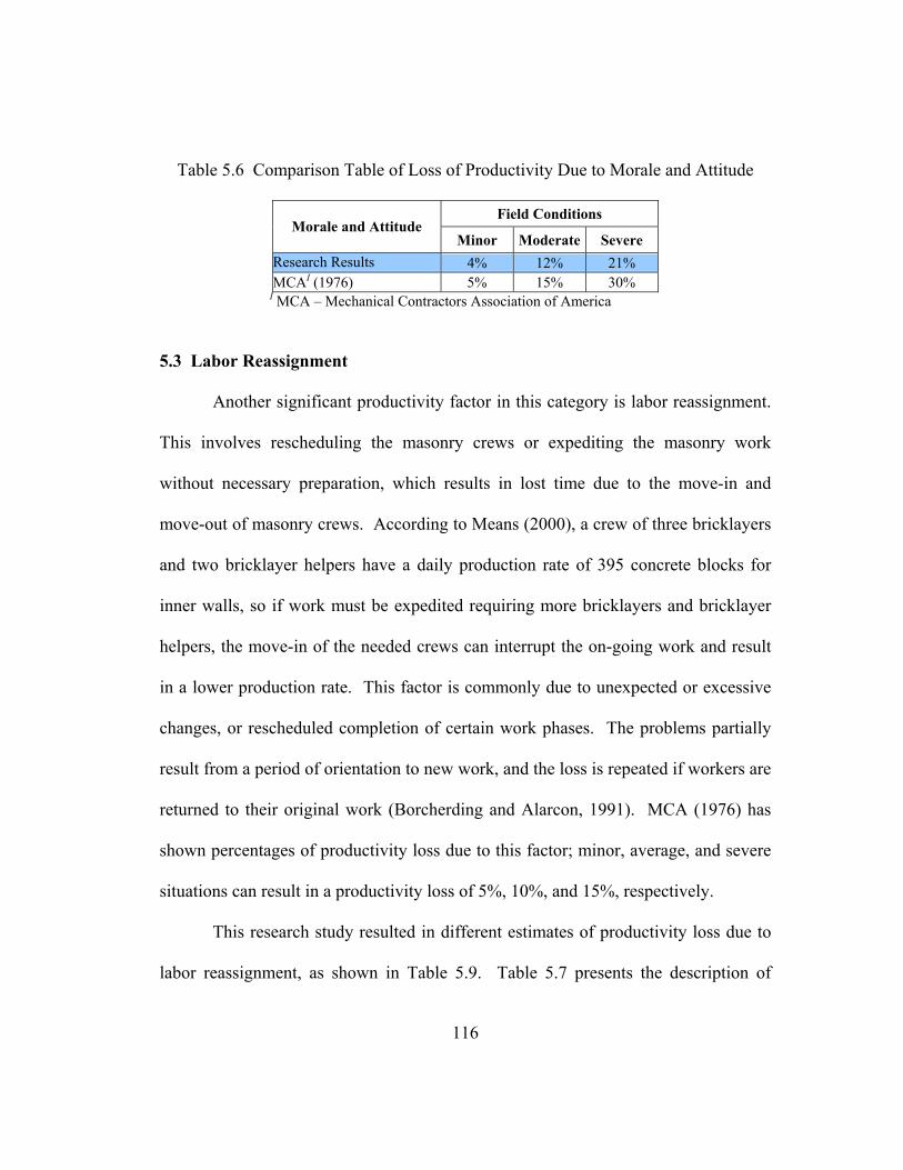
Table 5.6 Comparison Table of Loss of Productivity Due to Morale and Attitude
Field Conditions Morale and Attitude
Minor Moderate Severe Research Results 4% 12% 21% MCAI (1976) 5% 15% 30%
I MCA – Mechanical Contractors Association of America
5.3 Labor Reassignment
Another significant productivity factor in this category is labor reassignment.
This involves rescheduling the masonry crews or expediting the masonry work
without necessary preparation, which results in lost time due to the move-in and
move-out of masonry crews. According to Means (2000), a crew of three bricklayers
and two bricklayer helpers have a daily production rate of 395 concrete blocks for
inner walls, so if work must be expedited requiring more bricklayers and bricklayer
helpers, the move-in of the needed crews can interrupt the on-going work and result
in a lower production rate. This factor is commonly due to unexpected or excessive
changes, or rescheduled completion of certain work phases. The problems partially
result from a period of orientation to new work, and the loss is repeated if workers are
returned to their original work (Borcherding and Alarcon, 1991). MCA (1976) has
shown percentages of productivity loss due to this factor; minor, average, and severe
situations can result in a productivity loss of 5%, 10%, and 15%, respectively.
This research study resulted in different estimates of productivity loss due to
labor reassignment, as shown in Table 5.9. Table 5.7 presents the description of
116

standard field conditions for labor reassignment. The findings presented in Table 5.8
and Figure 5.3 show that if masonry workers move between job areas only once a
week, they will suffer an average productivity loss of five percent. This loss
dramatically increases to 12% once the workers need to move between job areas two
to three times per week. For severe field conditions, the workers are required to
move between job areas more than three times per week, which results in an average
productivity loss of 21%.
Table 5.7 Description of Standard Field Conditions for Labor Reassignment
Minor Moderate Severe Crews move once a week between job areas
Crews move 2-3 times/week between job areas
Crews move almost daily between jobs
Table 5.8 Percentage of Productivity Loss for Labor Reassignment
Field Conditions Labor Reassignment
Minor Moderate SevereMean 5 12 21 Median 5 10 20 Mode 5 10 20 Low 0 2 2 High 15 30 50 Range 15 28 48 Standard Deviation 3.1 6.4 11.4
117

Labor Reassignment
0
20
40
60
80
100
Minor Moderate Severe
Standard Field Conditions
% L
oss
of P
rodu
ctiv
ityHighMeanLow
Figure 5.3 Loss of Productivity Due to Labor Reassignment
Table 5.9 Comparison Table of Loss of Productivity Due to Labor Reassignment
Field Conditions
Labor Reassignment Minor Moderate Severe
Research Results 5% 12% 21% CCCI (1984) 10% 20% 30% MCAII (1976) 5% 10% 15%
I CCC – Contractor's Consultants Corporation II MCA – Mechanical Contractors Association of America
5.4 Crew Size Change
There have been several attempts to highlight factors associated with
resources and site management including crew size change or unbalanced crews.
Crew size change refers to changes that increase or decrease the optimum crew size,
resulting in inefficiency or workflow disruption. To determine the total cost of brick
installation, for example, Means (2000) specifies a crew of three bricklayers and two
bricklayer helpers with a daily output of approximately 1,800 common bricks for
118

eight inch solid walls. If a change order occurs with a short notice, resulting in a
shortage of one bricklayer, the crew will have a lower daily output and therefore
require a longer installation time. As stated in many studies, increasing the crew size
generally results in decreased productivity due to altering labor rhythm and breaking
up the original team effort (MCA, 1976; the Army Corps of Engineers, 1979;
Borcherding and Alarcon, 1991). Furthermore, impairment can occur due to limited
working space, diluted supervision, and lack of management support (MCA, 1976;
Borcherding and Alarcon, 1991). MCA (1976) refers to this factor as crew size
efficiency, and provides estimates of loss due to the effect of this factor. Minor,
moderate, and severe conditions of this factor typically generate productivity loss of
10%, 20%, and 30%, respectively. This paper, as stated earlier, provides very little
insight on database characteristics and data collection procedures.
This research study resulted in lower outcomes in estimates of productivity
loss. Table 5.10 presents the description of standard field conditions for crew size
change. Table 5.11 and Figure 5.4 show the research findings, and Table 5.12
presents a comparison of results from three studies. This research investigation
shows that there is a five percent productivity loss when crew size change exists once
per week. When the change increases its frequency to two to three times per week,
estimated loss of productivity has increased up to 11%. This rise increases to a 20%
productivity loss, when crew size change takes place almost daily. Even though these
mean averages are almost twice as low as other estimates, the means result from a
119

wide range of the estimates found in the study. This means that the crew size change
has a great range of impact on productivity and detailed investigations should be
conducted if severe conditions exist.
Table 5.10 Description of Standard Field Conditions for Crew Size Change
Minor Moderate Severe Crew size changes once/week
Crew size changes 2-3 times/week
Crew size changes almost daily
Table 5.11 Percentage of Productivity Loss for Crew Size Change
Field Conditions Crew Size Change
Minor Moderate SevereMean 5 11 20 Median 5 10 20 Mode 5 10 20 Low 0 3 5 High 15 25 50 Range 15 22 45 Standard Deviation 3.6 5.3 10.7
Crew Size Change
0
20
40
60
80
100
Minor Moderate Severe
Standard Field Conditions
% L
oss
of P
rodu
ctiv
ity
HighMeanLow
Figure 5.4 Loss of Productivity Due to Crew Size Change
120

Table 5.12 Comparison Table of Loss of Productivity Due to Crew Size Change
Field Conditions Crew Size Change
Minor Moderate Severe Research Results 5% 11% 20% CCCI (1984) 10% 30% 50% MCAII (1976) 10% 20% 30%
I CCC – Contractor's Consultants Corporation II MCA – Mechanical Contractors Association of America
5.5 Added Operations
Added operations or concurrent operations are of interest to many researchers
in the construction field. This factor includes any changed conditions that initiate
operations additional to ongoing masonry operations, which take place in a physically
limited space. The productivity loss usually results from stacking of the masonry
contractor’s own force working on an already planned sequence of operations. This
factor commonly exists when there is a need to accomplish additional work during
schedule acceleration. Estimates of productivity loss due to this factor are presented
by MCA (1976). Productivity losses of 5%, 15%, and 25% are suggested to
determine the effect if the conditions are minor, average, and severe, respectively.
This research study reveals similar results to those of MCA (1976), as shown
in Table 5.15. Additional findings are presented in Table 5.14 and Figure 5.5. An
average productivity loss of four percent is present when minor conditions exist or
there are additional operations once a week. When additional operations disrupt a
masonry crew two to three times a week, the estimated loss of productivity increases
121

to 11%. The severe condition involving additional operations more than three times a
week yields an average productivity loss of 18%. Table 5.13 presents the description
of standard field conditions for added operations.
Table 5.13 Description of Standard Field Conditions for Added Operations
Minor Moderate Severe Work disrupted once/week
Work disrupted 2-3 times/week
Work disrupted almost daily
Table 5.14 Percentage of Productivity Loss for Added Operations
Field Conditions Added Operations
Minor Moderate SevereMean 4 11 18 Median 5 10 16 Mode 5 10 20 Low 0 2 4 High 10 25 40 Range 10 23 36 Standard Deviation 1.9 5.4 8.3
Added Operation
0
20
40
60
80
100
Minor Moderate Severe
Standard Field Conditions
% L
oss
of P
rodu
ctiv
ity
HighMeanLow
Figure 5.5 Loss of Productivity Due to Added Operations
122

Table 5.15 Comparison Table of Loss of Productivity Due to Added Operations
Field Conditions Added Operations
Minor Moderate Severe Research Results 4% 11% 18% MCAI (1976) 5% 15% 25%
I MCA – Mechanical Contractors Association of America
5.6 Diverted Supervision
Findings from numerous research studies have highlighted productivity
factors related to management characteristics. A major factor associated with
management characteristics is diverted supervision or dilution of supervision. This
factor addresses changes that cause distraction of supervision from multiple on-going
activities, in order to analyze and plan changed work, stop and replan ongoing work
or reschedule work. Diverted supervision is critical when the masonry work is
accelerated or changed and a significant amount of instruction is required. MCA
(1976) estimates loss of productivity as 10%, 15%, and 25% for minor, average, and
severe situations.
This research investigation found that the results from this study are
somewhat lower than that of MCA (1976), as shown in Table 5.18. An average
productivity loss of six percent when diverted supervision occurs twice a week for
only two hours or less each as shown in Table 5.17 and Figure 5.6. An average
productivity loss of 13% arises where diverted supervision occurs two hours or less
123

daily. The loss increases to an average productivity loss of 22% when diverted
supervision exists daily for more than three hours. This factor has a broad range of
impacts for all conditions, likely depending upon the degree of management involved
in the masonry work at a certain period of time. For instance, in the morning, a
masonry crew needs advice or instructions for their work, requiring concentrated
attention from management at that time. This circumstance can generate high loss of
productivity. Table 5.16 presents the description of standard field conditions for
diverted supervision.
Table 5.16 Description of Standard Field Conditions for Diverted Supervision
Minor Moderate Severe 2 times/week, 1-2 hours Daily, 1-2 hours Daily, 4 hours or more
Table 5.17 Percentage of Productivity Loss for Diverted Supervision
Field Conditions Diverted Supervision
Minor Moderate SevereMean 6 13 22 Median 5 10 20 Mode 5 10 15 Low 0 2 5 High 15 30 55 Range 15 28 50 Standard Deviation 3.4 7.1 12.9
124

Diverted Supervision
0
20
40
60
80
100
Minor Moderate Severe
Standard Field Conditions
% L
oss
of P
rodu
ctiv
ityHighMeanLow
Figure 5.6 Loss of Productivity Due to Diverted Supervision
Table 5.18 Comparison Table of Loss of Productivity Due to Diverted Supervision
Field Conditions Diverted Supervision
Minor Moderate Severe Research Results 6% 13% 22% MCAI (1976) 10% 15% 25%
I MCA – Mechanical Contractors Association of America
5.7 Learning Curve
Researchers have shown an increasing interest in the learning curve as an
influence on productivity. The learning curve refers to a period of orientation
necessary to become familiar with new tasks or changed conditions, and increased
productivity is expected as the individual becomes more skilled and familiar with the
assigned tasks, tool locations, and work procedures (Borcherding and Alarcon, 1991).
For masonry construction, the production rate usually decreases while an individual is
125

obtaining more skills or becoming familiar with masonry work procedures, tool
locations and environment. This factor therefore refers to changes that cause
masonry workers to lose time while becoming familiar with and adjusting to new
work or a new environment.
Many publications have presented the effects of the learning curve. The
earliest published research on learning curve originated in the aircraft manufacturing
industry. In the industrial sector, Wright introduced the concept of learning curve for
production productivity. This rule is called Wright’s 80% rule and states that the
accumulated mean of operational times will be reduced to 80% of the expected value
computed based on the original mean, when doubling the number of identical
operations (Schwartzkopf, 1995). The equivalent of Wright’s 80% rule was later
found to be 87% to 93% in building operations of a repetitive nature (United Nations
Committee and Housing, 1965). More recent paper regarding learning curve was
published by MCA (1976). It presents quantitative evaluations to determine loss of
productivity due to this factor. The investigation determined losses of productivity of
5%, 15%, and 30% for minor, average, and severe conditions, respectively.
Findings from this research study have revealed different results compared to
other studies as shown in Table 5.21. Results from this study are summarized in
Table 5.20 and Figure 5.7. Table 5.19 presents the description of standard field
conditions for learning curve. Minor conditions representing change from one
masonry operation to another operation once a week yield an average productivity
126

loss of four percent. Moderate conditions exist with changes two to three times per
week, which has an average productivity loss of 11%. Severe conditions, in contrast,
indicate changes more than three times per week, which cause a high average
productivity loss of 18%.
Table 5.19 Description of Standard Field Conditions for Learning Curve
Minor Moderate Severe Once a week 2-3 times/week Daily
Table 5.20 Percentage of Productivity Loss for Learning Curve
Field Conditions
Learning Curve Minor Moderate Severe
Mean 4 11 18 Median 5 10 15 Mode 5 10 15 Low 0 2 4 High 9 25 50 Range 9 23 46 Standard Deviation 2.0 6.1 10.1
Learning Curve
0
20
40
60
80
100
Minor Moderate Severe
Standard Field Conditions
% L
oss
of P
rodu
ctiv
ity
HighMeanLow
Figure 5.7 Loss of Productivity Due to Learning Curve
127

Table 5.21 Comparison Table of Loss of Productivity Due to Learning Curve
Field Conditions Learning Curve
Minor Moderate Severe Research Results 4% 11% 18% CCCI (1984) 10% 23% 35% MCAII (1976) 5% 15% 30%
I CCC – Contractor's Consultants Corporation II MCA – Mechanical Contractors Association of America
5.8 Errors and Omissions
In recent years, construction researchers and practitioners have begun to
account for engineering errors and omissions. This factor represents changed
conditions involving mistakes or unclear instructions in drawings, technical
documents or supervisions; which cause lost time, out-of-sequence work, rework or
other work conflicts. Engineering errors and omissions can be both the cause and
effect of changes and commonly result in loss of productivity (Borcherding and
Alarcon, 1991). From the results presented in MCA (1976), it is evident that errors
and omissions cause productivity losses of one percent, three percent, and six percent
for minor, average, and severe situations, respectively.
From the evidence presented in this report, it is likely that errors and
omissions cause loss of productivity as much as and even more than four times higher
than the losses reported by MCA (1976), as shown in Table 5.24. Based upon studies
of impacted projects (Borcherding and Alarcon, 1991), the higher loss percentages
due to design constraints support the findings in this study rather than MCS’s very
128

low percentages. Table 5.22 presents the description of standard field conditions for
errors and omissions. Table 5.23 and Figure 5.8 present a summary of the research
investigations. It was found that errors and omissions taking place every two weeks
or more are considered minor and generate an average productivity loss of four
percent. Meanwhile, changed conditions every week or every one to two days are
classified as moderate and severe, respectively, and they produce an average
productivity loss of 11% and 19%, respectively.
Table 5.22 Description of Standard Field Conditions for Errors and Omissions
Minor Moderate Severe Every 2 weeks or more Every week Every 1 or 2 day(s)
Table 5.23 Percentage of Productivity Loss for Errors and Omissions
Field Conditions Errors and Omissions
Minor Moderate SevereMean 4 11 19 Median 5 10 15 Mode 5 10 15 Low 0 2 4 High 8 25 45 Range 8 23 41 Standard Deviation 1.9 5.8 9.6
129

Errors and Omissions
0
20
40
60
80
100
Minor Moderate Severe
Standard Field Conditions
% L
oss
of P
rodu
ctiv
ityHighMeanLow
Figure 5.8 Loss of Productivity Due to Errors and Omissions
Table 5.24 Comparison Table of Loss of Productivity Due to Errors and Omissions
Field Conditions Errors and Omissions
Minor Moderate Severe Research Results 4% 11% 19% MCAI (1976) 1% 3% 6%
I MCA – Mechanical Contractors Association of America
5.9 Beneficial Occupancy
One of the major field factors facing masonry contractors today is beneficial
occupancy. This factor focuses on changes that require the use of premises by the
owner prior to masonry work completion, restricted work access, or working close to
the owner’s personnel or equipment. The effect of this factor has been quantified by
MCA (1976). The estimated productivity losses of this factor are 15%, 25%, and
40% for minor, moderate, and severe conditions, respectively. These results are some
130

of the highest values among all factors presented in MCA (1976). This distinction
highlights the significant effect of this factor on labor productivity of mechanical
construction.
This research study has verified that beneficial occupancy does in deed have a
major impact on productivity in masonry construction. Table 5.25 presents the
description of standard field conditions for beneficial occupancy. Tables 5.26 and
5.27, and Figure 5.9 show analysis results of this study as well as a comparison
between results of this study and those of MCA (1976). Although the results from
this study are relatively lower than those of MCA (1976), they are higher than many
other factors in this research study. Findings from this study indicate that an average
productivity loss of seven percent exists when there is punch list work or minor
conditions. Beneficial occupancy can be considered as moderate when there is a
punch list and new work one week prior to the original completion date, causing an
average productivity loss of 14%. Severe conditions, however, involving numerous
crews and overtimes only a few days prior to the original completion date can
generate an average productivity loss of 25%.
Table 5.25 Description of Standard Field Conditions for Beneficial Occupancy
Minor Moderate Severe Punch list work
Punch list and new work one week prior to the original completion date
Many crews and overtime a few days prior to the original completion date
131

Table 5.26 Percentage of Productivity Loss for Beneficial Occupancy
Field Conditions Beneficial Occupancy
Minor Moderate SevereMean 7 14 25 Median 5 10 20 Mode 10 10 15 Low 0 0 1 High 20 40 63 Range 20 40 62 Standard Deviation 5.5 8.9 14.1
Beneficial Occupancy
0
20
40
60
80
100
Minor Moderate Severe
Standard Field Conditions
% L
oss
of P
rodu
ctiv
ity
HighMeanLow
Figure 5.9 Loss of Productivity Due to Beneficial Occupancy
Table 5.27 Comparison Table of Loss of Productivity Due to Beneficial Occupancy
Field Conditions Beneficial Occupancy
Minor Moderate Severe Research Results 7% 14% 25% MCAI (1976) 15% 25% 40%
I MCA – Mechanical Contractors Association of America
132

5.10 Joint Occupancy
Another factor currently of interest to masonry contractors is joint occupancy.
This factor deals with significant changes that require masonry work to be done while
other trades occupy the same area. In such a busy work area, for example,
productivity loss can result from loss of masonry tools or difficulty in locating brick
stacks. MCA (1976) has quantified loss of productivity due to this factor for
mechanical work. It shows that 5%, 12%, and 20% of productivity losses may exist
for minor, average, and severe conditions, respectively.
Compared to MCA (1976), results from this research study indicate higher
losses of productivity due to joint occupancy, as shown in Figure 5.10 and Tables
5.29 and 5.30. An average productivity loss of seven percent exists when a facility is
partly occupied and only one additional trade is working in the same area with the
masonry crew. The average loss increases up to 14% when a facility is partly
occupied and two or three trades are working in the same area. Even more severely,
there is an average productivity loss of 25% when a facility is fully in operation and
masonry work is on limited shifts. Table 5.28 presents the description of standard
field conditions for joint occupancy.
Table 5.28 Description of Standard Field Conditions for Joint Occupancy
Minor Moderate Severe Facility partly occupied, one trade working
Facility partly occupied, 2-3 trades working in the same area
Facility in operation, work on limited shifts
133

Table 5.29 Percentage of Productivity Loss for Joint Occupancy
Field Conditions
Joint Occupancy Minor Moderate Severe
Mean 7 14 25 Median 5 15 25 Mode 10 15 20 Low 0 0 4 High 20 35 50 Range 20 35 46 Standard Deviation 4.4 7.1 11.3
Joint Occupancy
0
20
40
60
80
100
Minor Moderate Severe
Standard Field Conditions
% L
oss
of P
rodu
ctiv
ity
HighMeanLow
Figure 5.10 Loss of Productivity Due to Joint Occupancy
Table 5.30 Comparison Table of Loss of Productivity Due to Joint Occupancy
Field Conditions Joint Occupancy
Minor Moderate Severe Research Results 7% 14% 25% MCAI (1976) 5% 12% 20%
I MCA – Mechanical Contractors Association of America
134

5.11 Site Access
There have been several attempts to highlight factors associated with
resources and site management, one of which is site access. This factor deals with
changes involving inconvenient access to masonry work areas, inadequate or
congested work spaces or remote materials storage. Productivity loss usually occurs
when additional work-hours are needed to demolish an existing physical structure, or
additional time is required to access a work area or materials storage for any reason
(Borcherding and Alarcon, 1991). MCA (1976) has presented estimates of the effect
of this factor. Findings from this investigation state that productivity losses due to
this factor are 5%, 12%, and 30% for minor, average, and severe conditions,
respectively.
The analysis of this research study, however, indicates that minor conditions,
involving convenient access to a work area four days per week or more or a distance
of less than 25 yards to materials storage, have an average productivity loss of seven
percent, as shown in Table 5.32 and Figure 5.11. This result shows the highest
impact among minor conditions compared with other studies, as shown in Table 5.33.
Moderate conditions involving convenient access to a work area two to three times
per week or a distance of 25 to 50 yards to materials storage, yield an average
productivity loss of 14% Additionally, when a masonry crew has extremely limited
access to a work area or a distance of more than 50 yards to material storage, the
analysis result indicates an average productivity loss of 27%. This factor signifies a
135

considerable impact to masonry productivity compared to other factors, and it is
essential that masonry practitioners be aware of any situations that can cause this
factor. Table 5.31 presents the description of standard field conditions for site access.
Table 5.31 Description of Standard Field Conditions for Site Access
Minor Moderate Severe 4 days/week, < 25 yards to materials storage
2-3 days/week, 25-50 yards to materials storage
Once/week, > 50 yards to materials storage
Table 5.32 Percentage of Productivity Loss for Site Access
Field Conditions Site Access
Minor Moderate SevereMean 7 14 27 Median 5 15 25 Mode 5 10 20 Low 0 0 0 High 15 30 60 Range 15 30 60 Standard Deviation 4.3 7.2 13.0
136

Site Access
0
20
40
60
80
100
Minor Moderate Severe
Standard Field Conditions
% L
oss
of P
rodu
ctiv
ityHighMeanLow
Figure 5.11 Loss of Productivity Due to Site Access
Table 5.33 Comparison Table of Loss of Productivity Due to Site Access
Field Conditions Site Access
Minor Moderate Severe Research Results 7% 14% 27% CCCI (1984) 5% 28% 50% MCAII (1976) 5% 12% 30%
I CCC – Contractor's Consultants Corporation II MCA – Mechanical Contractors Association of America
5.12 Logistics
Numerous investigations have presented several negative factors associated
with materials and tools availability or logistics. This factor involves changes that
cause an unsatisfactory supply of masonry materials by the owner or general
contractor, inability to control procurement, delivery or re-handling of substituted
materials, or difficulty controlling materials flow to work areas. It is conceivable that
137

materials and tools must be available for craftsmen to perform their work; otherwise,
loss of productivity can occur due to idle time or ineffective work. As logical
problems develop, consequential difficulties arise, including hoarding in-short-supply
items, and resequencing planned work to make use of available materials and tools
may arise (Borcherding and Alarcon, 1991). These obstacles and other problems
related to materials flow or materials procurement and delivery can cause loss of
productivity. Findings from several investigations have confirmed this fact.
MCA (1976) has proposed percentages of productivity loss due to logistics.
Losses of productivity are estimated to be as high as 10%, 25%, and 50% if the
conditions are minor, average, and severe, respectively. These high values show that
logistics is probably the most significant and extreme factor in construction. A more
recent research study conducted by Neil and Knack (1984) have quantified effects of
this factor using adjustment factors. Their findings indicate that, based on the
Houston, Texas fixed factors, loss of productivity due to this factor can range from
5% to 25% when the design is incomplete at the construction start-time or normal
lead times for items being processed. Borcherding et al. (1980) and Borcherding and
Garber (1981) have also measured lost time due to this factor and presented
subsequent effects on labor productivity.
The considerable influence of this factor on productivity has also been
quantified in this research study. Table 5.34 presents the description of standard field
conditions for logistics. Tables 5.35 and 5.36, and Figure 5.12 summarize results
138

from this research study and compare them with other significant studies. Minor
conditions involving one re-handling lifting or four-days-per-week materials
availability yield an average productivity loss of seven percent. Moderate conditions
requiring two to three re-handling lifting or two-to-three-days-per-week material
availability bear an average productivity loss of 15%. Severe conditions involving
more than three re-handling lifting or limited access time to materials bear an average
productivity loss of 26%. These numbers are relatively low compared to those of
MCA (1976), but somewhat similar to those of Neil and Knack (1984).
Table 5.34 Description of Standard Field Conditions for Logistics
Minor Moderate Severe 1 re-handling lifting, 4 days/week material availability
2 re-handling lifting, 2-3 days/week material availability
> 3 re-handling lifting, limited time
Table 5.35 Percentage of Productivity Loss for Logistics
Field Conditions Logistics
Minor Moderate SevereMean 7 15 26 Median 6 15 25 Mode 10 10 20 Low 0 0 0 High 15 33 73 Range 15 33 73 Standard Deviation 3.6 7.1 14.0
139

Logistics
0
20
40
60
80
100
Minor Moderate Severe
Standard Field Conditions
% L
oss
of P
rodu
ctiv
ityHighMeanLow
Figure 5.12 Loss of Productivity Due to Logistics
Table 5.36 Comparison Table of Loss of Productivity Due to Logistics
Field Conditions Logistics
Minor Moderate Severe Research Results 7% 15% 26% MCAI (1976) 10% 25% 50% Neil and Knack (1984) 5% N/A 25%
I MCA – Mechanical Contractors Association of America
5.13 Fatigue
Fatigue of crew members is recognized as one of the major productivity
factors and is interrelated with labor and morale. Fatigue is a physical or mental
condition involving physical or mental stress, unusual physical exertion or long
periods of overtime. This factor usually denotes changed conditions that entail
physical exertion or other fatiguing activities causing lost time when an original plan
resumes. A remote project can also result in fatigue because crews need to travel
140

long distances to work (Bocherding and Alarcon, 1991). Furthermore, heavy
materials and rework due to changes or engineering errors can cause physical fatigue.
Although using large and heavy masonry units can increase productivity, it may result
in a decrease in productivity if a long period of overtime exists. Findings from
MCA(1976) have supported the notion that fatigue can contribute to significant loss
of productivity. MCA (1976) estimates that, for minor, average, and severe
conditions, losses of productivity are 8%, 10%, and 12%, respectively.
This research study revealed percentages significantly different from those of
MCA (1976), as shown in Tables 5.38 and 5.39, and Figure 5.13. Table 5.37 presents
the description of standard field conditions for fatigue. For minor conditions, when
fatigue of crew members develops once a week, an average productivity loss of five
percent exists, relatively small compared to one of MCA (1976). When disruptions
proceed causing fatigue of crew members two or three times a week, the loss
significantly increases to 11% on average. The rise increases to an average
productivity loss of 20%, when the disruptions persist more than three times a week.
It is recognized that productivity loss due to effects of fatigue significantly increases
when disruptions are present more than once a week, and proceeds with a high rate of
productivity loss if the disruptions continue.
Table 5.37 Description of Standard Field Conditions for Fatigue
Minor Moderate Severe Once/week 2-3 times/week Every day for more than 1 week
141

Table 5.38 Percentage of Productivity Loss for Fatigue
Field Conditions
Fatigue Minor Moderate Severe
Mean 5 11 20 Median 5 10 20 Mode 5 10 20 Low 0 1 4 High 15 25 50 Range 15 24 46 Standard Deviation 3.7 6.2 10.6
Fatigue
0
20
40
60
80
100
Minor Moderate Severe
Standard Field Conditions
% L
oss
of P
rodu
ctiv
ity
HighMeanLow
Figure 5.13 Loss of Productivity Due to Fatigue
Table 5.39 Comparison Table of Loss of Productivity Due to Fatigue
Field Conditions Fatigue
Minor Moderate Severe Research Results 5% 11% 20% MCAI (1976) 8% 10% 12%
I MCA – Mechanical Contractors Association of America
142

5.14 Work Sequence
Disrupted work sequence or ripple effect is one of the most significant
problems caused by changes. This factor highlights changes in other trades that
consequentially affect the masonry contractor’s own work, including rescheduling or
changes in work sequence. Also, a disruption exists when there is significant lack of
resources, when the work is performed in a congested area, or when out-of-sequence
work is required (Thomas and Oloufa, 1995). MCA (1976) has presented percentages
of productivity loss due to this ripple effect. It shows that productivity losses of 10%,
15%, and 20% are present for minor, average, and severe conditions. A recent
research study performed by Thomas and Oloufa (1995) to determine the relationship
between labor productivity and disruptions also accounted for ripple effect. Findings
from this study indicate that one disruption per week results in a nine percent loss of
performance for an average project. When the ripple effect is present, the required
work-hours increase by an average order of magnitude of almost three, and as much
as five for disrupted projects.
In this research study, particular efforts were called for in determining the
estimates due to the effects of the disruption. Table 5.40 presents the description of
standard field conditions for work sequence. Findings obtained from research
investigations are presented in Figure 5.14, and Tables 5.41 and 5.42. The results
show that minor conditions involving disruptions due to another trade or one change
per week cause an average productivity loss of six percent. When two to three trades
143

or changes per week disrupt masonry work, an average percent loss of productivity is
approximately 14% similar to one of MCA (1976). However, the average loss
increases significantly to approximately 23% when more than three trades or changes
per week are present. This result is supported by the earlier findings of Thomas and
Oloufa (1995).
Table 5.40 Description of Standard Field Conditions for Work Sequence
Minor Moderate Severe One trade, one change/week
2 trades, 2-3 changes/week
Multiple trades, many changes
Table 5.41 Percentage of Productivity Loss for Work Sequence
Field Conditions Work Sequence
Minor Moderate SevereMean 6 14 23 Median 5 10 20 Mode 5 10 20 Low 0 0 5 High 15 35 50 Range 15 35 45 Standard Deviation 3.8 7.5 11.7
144

Work Sequence
0
20
40
60
80
100
Minor Moderate Severe
Standard Field Conditions
% L
oss
of P
rodu
ctiv
ityHighMeanLow
Figure 5.14 Loss of Productivity Due to Work Sequence
Table 5.42 Comparison Table of Loss of Productivity Due to Work Sequence
Field Conditions Work Sequence
Minor Moderate Severe Research Results 6% 14% 23% MCAI (1976) 10% 15% 20% Thomas and Oloufa (1995) 9% N/A 23%
I MCA – Mechanical Contractors Association of America
5.15 Overtime
An extensive literature review shows that scheduled overtime can result in
significant productivity loss in construction. This factor addresses any changed
conditions that require overtime causing masonry workers to perform less efficiently
than expected under the normal schedule, a schedule of eight-hours-per-day, five-
days-per-week. The productivity loss normally results from physical fatigue, poor
mental attitude and management inefficiency (Borcheding and Alarcon, 1991).
145

Overtime may also results in poor workmanship, while increasing accidents and
absenteeism.
In recent years, there have been numerous investigations involved with
overtime. Estimates presented by MCA (1976) show that losses of productivity due
to this factor are 10%, 15%, and 20% for minor, average, and severe conditions,
respectively. Business Roundtable (1980) states that overtime losses are not
automatic but can range from none to approximately 25% for crews where there are
no other factors involved (Thomas and Raynar 1994). In an effort to quantify
productivity loss, Neil and Knack (1984) have shown that, based on the Houston,
Texas fixed factors, there is a loss of productivity of about 10% for the following
schedules: seven days of eight hours, six days of nine hours, and five days of 10
hours. Furthermore, a loss of productivity of 20% occurs for the following work
schedules: seven days of 10 hours, six days of 11 hours, and five days of 12 hours.
Another significant study conducted by NECA (1989) indicates only small
productivity losses when working isolated amounts of overtime. This study provides
productivity data as a function of work days per week and work hours per day. It also
introduces several tables showing a wide range of productivity loss data based on
various numbers of work days per week and hours per work days.
Several extensive studies of the effects of scheduled overtime were sponsored
by CII (CII, 1988; Thomas, 1990; Thomas and Raynar 1994). The findings of CII
(1988) indicate that productivity loss from working overtime is not automatic and it is
146

possible to work 60-hour weeks without serious productivity losses for several week
periods of spot overtime (Schwartzkopf, 1995). This shows that productivity loss
from short periods of overtime can be controlled by implementing effective
management and support. Furthermore, Thomas and Raynar (1994) recently found
that on average there is about a 15% loss of efficiency for weeks consisting of 50 and
60 hours.
Although these studies have varying results, the range of time is used for
comparison purposes, and the results are shown in Table 5.45. Findings from several
studies, including this one, are fairly consistent considering that each study considers
a different combination of projects, trades, localities, and time. Table 5.44 and Figure
5.15 show a summary of this research study based on three different field conditions.
Table 5.43 presents the description of standard field conditions for overtime. Minor
conditions, referring to overtime of less than five hours per week for two consecutive
weeks or less, result in an average productivity loss of seven percent. Moderate
conditions, involving overtime of five to ten hours per week for three to five
consecutive weeks, can generate an average productivity loss of 15%. More
importantly, severe conditions involving overtime 11 hours or more per week for
more than five consecutive weeks produce an average productivity loss of 24%. If
there is a conflict condition, the higher number of hours or weeks may be applied.
For instance, if there are 11-hours-per-week overtime for two consecutive weeks, this
would be considered as a severe condition.
147

Table 5.43 Description of Standard Field Conditions for Overtime
Minor Moderate Severe < 5 hours/week, 1-2 consecutive weeks
5-10 hours/week, 3-5 consecutive weeks
> 10 hours/week, > 5 consecutive weeks
Table 5.44 Percentage of Productivity Loss for Overtime
Field Conditions Overtime
Minor Moderate SevereMean 7 15 24 Median 5 15 22 Mode 5 10 20 Low 0 0 3 High 15 35 50 Range 15 35 47 Standard Deviation 4.2 7.4 11.3
Overtime
0
20
40
60
80
100
Minor Moderate Severe
Standard Field Conditions
% L
oss
of P
rodu
ctiv
ity
HighMeanLow
Figure 5.15 Loss of Productivity Due to Overtime
148

Table 5.45 Comparison Table of Loss of Productivity Due to Overtime
Field Conditions Overtime
Minor Moderate Severe Research Results 7% 15% 24% BRTI (1980) 0% N/A 25% MCAII (1976) 10% 15% 20% Neil and Knack (1984) N/A 10% 20% Thomas and Raynar (1994) N/A 15% N/A
I BRT – Business Roundtable II MCA – Mechanical Contractors Association of America
5.16 Weather or Environment
An extensive review of the relevant studies has shown that external conditions
in construction have significantly contributed to loss of productivity. Recently,
numerous research studies have focused on adverse weather and environment, one of
the most critical productivity factors in construction. This factor refers to differing
site conditions from the estimating base due to natural forces such as severe weather,
high humidity, high wind velocity, precipitation or snow, dusty or noisy conditions,
or a combination of those. It is conceivable that adverse weather greatly affects
construction operations and workers both physically and physiologically, thus
slowing down the work. The impacts of adverse weather vary dramatically, but the
greatest impacts are upon outside operations, particularly those involving
earthmoving and temperature-and-weather-sensitive material such as concrete and
mortar. In masonry construction, productivity is significantly influenced by low
temperatures.
149

A significant number of research studies have focused on this factor. Several
studies show that there is almost no effect on productivity until the temperature drops
below 40ºF (Grimm and Wagner, 1974; Heather and Summers, 1996; NECA, 1974).
In the year 1974, Grimm and Wagner established relationships between masonry
productivity and temperature and humidity. Research results showed that masonry
“productivity was found to decline as the temperature or humidity deviated from 75°F
and 60%” (Grimm and Wagner, 1974). Based on the temperature of 75ºF and the
humidity of 60%, they estimated a productivity loss of 10% and 22% when the
temperature increased or decreased 5ºF and 10ºF, respectively. Moreover, when the
temperature increased or decreased 15ºF, a productivity loss of about 30% was
estimated. Another significant study published by MCA (1976) provides estimates of
the effects of weather change. If the conditions are minor, average, and severe, the
loss of productivity is 10%, 20%, and 30%, respectively.
In 1984, Neil and Knack presented adjustment factors for severe weather.
Their findings show that productivity loss ranges from 5% to 25% when heavy
protective clothing is required, heat and humidity are at discomfort levels, and/or
wind and precipitation slow down workers activities, based on the Edmonson fixed
factors for Houston, Texas. Furthermore, Koehn and Brown (1985) have determined
two nonlinear equations showing relationships of productivity and temperature an
humidity based on productivity data from other sources, such as NECA (1974) and
Grimm and Wagner (1974) studies. A more recent research study conducted by
150

Thomas and Yiakoumis (1987) presents the factor model of construction productivity
and investigates the effects of adverse weather on productivity based on three
construction activities: masonry construction, structural steel erection, and framework
erection.
Results from other research studies, including those of this research study, are
presented in a comparison matrix as shown in Table 5.48. Although the sources are
not directly related, a range of factors can be considered for comparison. These
studies present results derived from both cold and hot weather. In this research study,
field conditions were classified by the difference between the expected temperature
and the actual temperature. Table 5.46 presents the description of standard field
conditions for weather and environment. Minor, moderate and severe conditions
indicate a temperature difference of 5ºF, 10ºF and 15ºF, respectively. Based on
research results presented in Table 5.47 and Figure 5.16, the analysis shows an
average productivity loss of 6%, 12% and 22% in minor, moderate and severe
conditions, respectively.
Table 5.46 Description of Standard Field Conditions for Weather or Environment
Minor Moderate Severe Expected temp. +5F in summer or -5F in winter
Expected temp. +10F in summer or -10F in winter
Expected temp. +15F in summer or -15F in winter
151

Table 5.47 Percentage of Productivity Loss for Weather or Environment
Field Conditions Weather or Environment Minor Moderate Severe
Mean 6 12 22 Median 5 10 20 Mode 5 10 20 Low 0 0 2 High 20 25 50 Range 20 25 48 Standard Deviation 4.6 6.2 10.9
Weather or Environment
0
20
40
60
80
100
Minor Moderate Severe
Standard Field Conditions
% L
oss
of P
rodu
ctiv
ity
HighMeanLow
Figure 5.16 Loss of Productivity Due to Weather or Environment
Table 5.48 Comparison Table of Loss of Productivity Due to Weather or
Environment
Field Conditions Weather or Environment
Minor Moderate Severe Research Results 6% 12% 22% Grimm (1974) 10% 22% 30% MCAI (1976) 10% 20% 30%
I MCA – Mechanical Contractors Association of America
152

5.17 Summary
This chapter outlined research findings and presented discussions of 16 field
disruptions that commonly occur in masonry construction based on a national survey
conducted throughout the U.S. For each factor, the research findings presented low,
mean, and high percentages of productivity loss due to disruptions with minor,
moderate, and severe conditions. Table 5.49 presents a summary of the findings in
descending order sorted by the means of minor, moderate, and severe conditions,
respectively. This table shows that logistics, overtime, and site access are the most
influencing disruptions in masonry building construction. In addition, beneficial and
joint occupancy are also significant disruptions for masonry contractors. In this
chapter, findings from a number of studies were also discussed in comparison with
the analysis results. The next chapter will test the research findings from this chapter
through the development and validation of a model to determine loss of productivity.
153

Table 5.49 Summary of Percentages of Productivity Loss Due to Field Disruptions
Estimated percentage of productivity loss (%), if the disruption is …
Minor Moderate Severe No. Field Disruptions
Low Mean High Low Mean High Low Mean High1 Logistics 0 7 15 0 15 33 0 26 73 2 Overtime 0 7 15 0 15 35 3 24 50 3 Site Access 0 7 15 0 14 30 0 27 60 4 Beneficial Occupancy 0 7 20 0 14 40 1 25 63 5 Joint Occupancy 0 7 20 0 14 35 4 25 50 6 Work Sequence 0 6 15 0 14 35 5 23 50 7 Diverted Supervision 0 6 15 2 13 30 5 22 55 8 Weather or Environment 0 6 20 0 12 25 2 22 50 9 Congestion 0 5 10 2 12 25 5 24 50 10 Labor Reassignment 0 5 15 2 12 30 2 21 50 11 Crew Size Change 0 5 15 3 11 25 5 20 50 12 Fatigue 0 5 15 1 11 25 4 20 50 13 Morale and Attitude 0 4 9 0 12 30 0 21 55 14 Errors and Omissions 0 4 8 2 11 25 4 19 45 15 Added Operations 0 4 10 2 11 25 4 18 40 16 Learning Curve 0 4 9 2 11 25 4 18 50
154

CHAPTER VI
VALIDATION OF THE HYPOTHESIS AND
MODEL DEVELOPMENT AND VALIDATION
Significant findings presented in the previous chapter were utilized in the
model development. This chapter presents the development and validation of the
research model, created to estimate loss of productivity due to an impact of various
field disruptions. Additionally, this chapter addresses practical steps for calculating
loss of productivity based on the model obtained. Questionnaire issues, data
collection, and data analysis for the model validation are also discussed. This chapter
begins by detailing a validation of the research hypothesis and the development and
implementation of the model, followed by model validation processes.
6.1 Validation of the Research Hypothesis
The hypothesis indicates that there are statistically significant differences
among productivity loss of different severity levels of field conditions in a masonry
building construction project, and considerable attention has been directed toward a
validation of this hypothesis. In this study, the different severity levels of field
conditions refer to three standard field conditions, minor, moderate, and severe. The
mean differences of percentages of productivity loss (%PL) of these three standard
conditions were tested through the use of the one-way ANOVA option in the SPSS®
155

9.05 for WindowsTM. Sixteen ANOVA tables presenting the F-statistic and
significance of three standard conditions for the 16 field disruptions were generated,
and major findings from the tables are summarized in Table 6.1.
This table shows that the F-statistics are higher than 1.0 and the significances
are less than 0.05 for all field disruptions. In other words, the F-statistics are
extremely high and the significances are extremely low. That is, the research
hypothesis is not rejected or there are statistically significant differences among
means of productivity loss for the three different standard conditions for all
disruptions. This table also presents means of %PL for the three standard conditions
of all disruptions. The findings show that %PL increases as the level of severity in
the construction field increases.
156

Table 6.1 Summary of Findings from ANOVA
No. Field Disruptions Field Conditions
Mean of %PL
Standard Deviation
Sample Size F-Statistic Significance
1 Congestion Minor 5 2.91 112 174.71 0.000Moderate 12 5.79 110Severe 24 11.92 114
2 Morale and Attitude Minor 4 2.03 94 105.28 0.000Moderate 12 7.40 113Severe 21 11.93 112
3 Labor Reassignment Minor 5 3.14 112 133.01 0.000Moderate 12 6.35 113Severe 21 11.41 113
4 Crew Size Change Minor 5 3.61 115 124.61 0.000Moderate 11 5.26 110Severe 20 10.66 113
5 Added Operations Minor 4 1.89 95 150.33 0.000Moderate 11 5.35 112Severe 18 8.29 108
6 Diverted Supervision Minor 6 3.40 115 107.83 0.000Moderate 13 7.07 114Severe 22 12.88 112
7 Learning Curve Minor 4 2.04 98 104.03 0.000Moderate 11 6.13 114Severe 18 10.10 110
8 Errors and Omissions Minor 4 1.88 97 129.61 0.000Moderate 11 5.84 114Severe 19 9.57 110
9 Beneficial Occupancy Minor 7 5.50 116 93.25 0.000Moderate 14 8.93 115Severe 25 14.14 114
10 Joint Occupancy Minor 7 4.43 116 150.98 0.000Moderate 14 7.09 116Severe 25 11.27 114
11 Site Access Minor 7 4.28 111 141.35 0.000Moderate 14 7.24 112Severe 27 12.96 116
12 Logistics Minor 7 3.62 108 121.57 0.000Moderate 15 7.10 111Severe 26 14.02 116
13 Fatigue Minor 5 3.70 112 110.68 0.000Moderate 11 6.25 111Severe 20 10.63 114
14 Work Sequence Minor 6 3.84 116 120.83 0.000Moderate 14 7.51 116Severe 23 11.74 113
15 Overtime Minor 7 4.16 115 137.72 0.000Moderate 15 7.36 115Severe 24 11.31 114
16 Weather or Environment Minor 6 4.65 116 126.48 0.000Moderate 12 6.25 111Severe 22 10.88 113
157

These findings were determined based on violations of two out of three basic
assumptions for the one-way ANOVA. The first assumption was that the population
distributions on the response variable were normal for all population groups.
However, in this study, the distributions of means of productivity loss for standard
conditions of the disruptions were not normal and had skewness ranging from -0.48 to
1.01 as shown in the summary of data analyses results shown in Appendix F. The
second assumption stated that the standard deviations of the population distributions
were equal for all population groups. However, the standard deviations of means of
productivity loss range from 1.88 to 14.14, as shown in Table 6.1. The last
assumption was that independent samples were collected from populations of all
groups. The samples in this study were randomly gathered, and thereby meeting this
assumption.
6.2 Model Development
One of the significant objectives of this research study is to develop a
practical and effective model representing estimates of the negative effects of field
disruptions on productivity. In this research study, particular attention was given to
develop a model by considering its accuracy, completeness, and ease of
implementation. The model includes mean, median, low, and high values of possible
losses of productivity determined from the analyses. The numerical means and
medians presented herein are used as estimates of productivity loss due to field
158

disruptions because they are the most accurate point estimates of the sample
population in this study. The low and high values are the minimum and maximum
values, respectively, after several outliers and extremes were discarded from the
database. The model representing mean, median, low, and high values of percentages
of productivity loss due to the effects of field disruptions was constructed as shown in
Table 6.2.
For practical use of the model, a copy of the standard conditions and
definitions of field disruptions should be attached. These documents will assist in
understanding the concept and terminologies of the model, as well as interpreting this
model to a specific construction jobsite. Additionally, computational examples
showing a process of implementing the model for estimating loss of productivity can
be attached as well for reference. Along with these documents, the model is
anticipated to be very useful for masonry practitioners in quantifying loss of
productivity due to the effects of field disruptions.
159

Table 6.2 Model Presenting Low, Median, Mean, and High Values of Percentages of Productivity Loss
Low Median Mean High Low Median Mean High Low Median Mean High1 Congestion 0 5 5 10 2 10 12 25 5 20 24 502 Morale and Attitude 0 5 4 9 0 10 12 30 0 20 21 553 Labor Reassignment 0 5 5 15 2 10 12 30 2 20 21 504 Crew Size Change 0 5 5 15 3 10 11 25 5 20 20 505 Added Operations 0 5 4 10 2 10 11 25 4 16 18 406 Diverted Supervision 0 5 6 15 2 10 13 30 5 20 22 557 Learning Curve 0 5 4 9 2 10 11 25 4 15 18 508 Errors and Omissions 0 5 4 8 2 10 11 25 4 15 19 459 Beneficial Occupancy 0 5 7 20 0 10 14 40 1 20 25 63
10 Joint Occupancy 0 5 7 20 0 15 14 35 4 25 25 5011 Site Access 0 5 7 15 0 15 14 30 0 25 27 6012 Logistics 0 6 7 15 0 15 15 33 0 25 26 7313 Fatigue 0 5 5 15 1 10 11 25 4 20 20 5014 Work Sequence 0 5 6 15 0 10 14 35 5 20 23 5015 Overtime 0 5 7 15 0 15 15 35 3 22 24 5016 Weather or Environment 0 5 6 20 0 10 12 25 2 20 22 50
Field Disruptions Moderate SevereNo.Estimated percentage of productivity loss (%), if the disruption is …
Minor
160
160

6.3 Implementation of the Model
The quantitative information provided in the model shows analysis results
that can be utilized and modified to better estimate the required work-hours
needed to perform certain work in field conditions that differ from original
expectations. The estimators can also determine the increase in the required
masonry work-hours, if project changes occur or field disruptions that are beyond
the control of the masonry contractor are present. The following information is
presented to propose a better understanding of how to apply the results. In this
study, since the means given for any field disruptions are derived from the effects
of that specific disruption with no effects of other disruptions involved, an
additive approach is adopted to determine the effects of multiple field
disruptions. The additive approach was used in this study because it was
recommended and implemented by Neil and Knack (1984) to predict labor
productivity. It was also commonly used to quantify the total productivity loss
due to mechanical disruptive factors presented by MCA (1976).
To estimate the impact of field disruptions in this study, there are two
classification methods based on whether the factors are applied prospectively or
retrospectively (Dieterle and DeStephanis, 1992). If one would like to
prospectively estimate the lost work-hours (LWH) for anticipated differences
after a contract award, the estimated %PL of expected factors should be added
and multiplied by the estimated work-hours (EWH), as shown in Equation 6.1.
161

On the other hand, if one would like to retrospectively quantify the lost work-
hours for construction claims, the estimated %PL of actual factors should be
added and then applied in Equation 6.2. One can also employ Equations 6.3 to
6.5 to retrospectively quantify total lost work-hours (TLH), actual work-hours
(AWH), and unexplained hours (UPH), respectively.
Prospectively
LWH = EWH x (%PL) (Equation 6.1)
Retrospectively
LWH = TWH – [TWH / (1 + %PL)] (Equation 6.2)
TLH = TWH – EWH (Equation 6.3)
AWH = TWH – LWH (Equation 6.4)
UPH = TLH – LWH (Equation 6.5)
Where: LWH = Lost Work-hours EWH = Estimated Work-hours
%PL = Percentage of Productivity Loss TWH = Total Work-hours
TLH = Total Lost Hours AWH = Actual Work-hours
UPH = Unexplained Hours
162

The following examples are presented to promote a better understanding of
how to use the model and the formulas, and an additive approach is adopted to
determine additional work-hours due to several field disruptions. Example 1 shows
that if the expected number of work-hours lost due to moderate congestion and
moderate diverted supervision is 250 hours for a 1,000-hour job, then the total
estimated work-hours required to perform the masonry work is 1,250 hours. With the
same disruptions, but retrospectively, example 2 shows that if the actual work-hours
equals 1,500 hours and the original work-hours was 1,000 hours, then the total lost
work-hours is 500 hours. The total lost work-hours include two components: 300 lost
work-hours due to differing field conditions that were beyond the control of the
masonry contractor, and 200 unexplained work-hours probably to be absorbed by the
masonry contractor. As a result, the actual work-hours required for the masonry work
was only 1,200 hours.
Example 1: To prospectively estimate the lost work-hours due to field
disruptions.
Before or during the masonry construction, the estimator figures the total
estimated work-hours at 1,000 hours, and moderate congestion and moderate
diverted supervision are expected. The expected work-hours lost and total
predicted work-hours required for the work can be determined as follows.
163

A. Total estimated masonry work-hours (EWH) = 1,000 hours
B. Field factors (means from the model)
No. 1 Congestion (Moderate) shows an average productivity loss of 12%
No. 6 Diverted Supervision (Moderate) shows an average productivity
loss of 13%
Total percentage of productivity loss (%PL) = 12% + 13% = 25% (or 0.25)
C. Expected work-hours lost due to the anticipated field factors
(LWH) = 1,000 x 0.25 = 250 hours
D. Total predicted work-hours required to perform the work
(A + C) = 1,000 + 250 = 1,250 hours
Example 2: To retrospectively estimate the lost work-hours due to field
disruptions.
After completion of the masonry work, the estimator determines that the actual
work-hours equals 1,500 hours, whereas the original estimated work-hours was
1,000 hours. During the masonry construction, moderate congestion and
moderate diverted supervision were present. The lost work-hours can be
determined as follow.
A. Total estimated masonry work-hours (EWH) = 1,000 hours
B. Total actual masonry work-hours (TWH) = 1,500 hours
C. Total lost work-hours (TLH) = 1,500 – 1,000 = 500 hours
164

D. Field factors (means from the model)
No. 1 Congestion (Moderate) shows an average productivity loss of 12%
No. 6 Diverted Supervision (Moderate) shows an average productivity
loss of 13%
Total percentage of productivity loss (%PL) = 12% + 13% = 25% (or 0.25)
E. Work-hours lost due to the field factors (LWH) = 1,500 – [1,500/(1+0.25)]
= 300 hours
F. Work-hours lost due to unexplained conditions (UPH) = 500 – 300
= 200 hours
G. Actual work-hours required without disruptions (AWH) = 1,500 – 300
= 1,200 hours
6.4 Model Validation Questionnaire
The primary goal of the model validation process is to determine the accuracy
of the model based on actual masonry construction projects. Particular efforts were
made in the development of the validation questionnaire and data collection. Based
on the criteria discussed in Section 3.7.2, the researcher paid close attention to several
aspects of the validation questionnaire including its accuracy, completeness, and
understanding, while maintaining an appropriate time frame for each interview
session. The researcher felt that an interview of less than one hour was the proper
165

time frame to allow the researcher to describe all necessary information to the
participant and to gather all necessary data needed for the validation analysis. The
essential information shared with the participant during the interview involved
research objectives, benefits of this research study, questionnaire objectives, and
characteristics of the questionnaire.
To facilitate the interview, the validation questionnaire was developed. The
questionnaire involved both open-ended and closed-ended questions as well as the list
of the 16 field disruptions and the standard conditions. The primary objective of the
survey was to collect essential data needed for further analyses, so the questionnaire
was classified into two parts. The first part of the questionnaire involved respondent
and project profiles; it was partly adopted from the questionnaire conducted for the
national survey study. Questions associated with the respondent profile basically
included the respondent’s position, contact information, and number of years of
experience in masonry construction. Questions associated with the project profile
primarily involved a project location, type of the project, project cost, and status of
the project. The status of the project referred to “ongoing” or “completed.” To better
understand the nature of project characteristics for future analyses and
recommendations, this part of the questionnaire included other questions related to
project characteristics such as original and actual project durations, an incidence of
166

project change orders, and a status of a project budget being “within” or “over”
budget.
The second part of the questionnaire primarily involved two major
components: masonry field disruptions and work-hours of the masonry crew during a
certain period of time frame. Part of the questionnaire is shown in Figure 6.1. Based
on the field disruptions and standard conditions, the researcher basically asked the
participant whether any disruptions existed during the masonry work execution
(Question B10). If so, the participant was expected to provide a list of the field
disruptions associated with field conditions and a frequency of the incidence.
Although it is generally necessary to provide a proof of the field conditions in a
disputed case in litigation, providing such proof is out of the scope of this research
study. The information in this study was therefore based on a database of the
participant, oral evidence, or experience of the participant.
In accordance with the information given by the participant, the researcher
determined whether the disruptions had occurred “very often” or “sometimes.” If the
incidence was “very often,” the factor would be included in the analysis; otherwise,
the researcher would postulate that the particular factor was a normal field condition,
generally found and accepted in masonry construction. Thus, that particular factor
would not be included in the analysis.
167

bas
wo
be
wa
imp
B.6 What was the original estimated work-hours for the masonry work? ________ hours
B.7 What was the actual work-hours for the masonry work? ________ hours
B.8 How do you rate the incidence of change orders on this masonry work?
□ Above average □ Average □ Below average
B.9 How do you rate the amount of rework on this masonry work?
□ Above average □ Average □ Below average
B.10 What were major field factors affecting masonry productivity on this project?
What was their condition level? (See the attachment for factor numbers and condition
levels.) How often were the disruptions present?
Factor
No.
Field Condition
Frequency of the Incidence
Time Frame of
the Incidence
□ Minor □ Moderate □ Severe □ Very often □ Sometimes
□ Minor □ Moderate □ Severe □ Very often □ Sometimes
□ Minor □ Moderate □ Severe □ Very often □ Sometimes
Figure 6.1 Part of the Validation Questionnaire Involving Field Disruptions and
Work-hours of Masonry Crew
The participant was also required to provide a time frame of the incidence
ed on his or her database or direct experience with the project. If the masonry
rk experienced a field disruption during most of the work period, the factor would
included in the analysis. If the masonry work encountered a field disruption that
s not for the whole period of the work, a proportional approach would be
lemented to determine work-hours used for calculating loss of work-hours. For
168

instance, if expected work-hours of the masonry crew is 1,000 hours and it is assumed
that during only 60% of the total work-hours congestion was experienced, only 600
hours of the estimated work-hours are appropriated as expected work-hours used for
further calculation. In this research study, none of the participants provided physical
evidence of the time frame of an incidence, so the data obtained were based on his or
her direct experience and the researcher’s judgment. The participant was also
welcome to provide additional field disruptions that existed at the construction field,
if not included in the given list of the 16 field disruptions. One participant suggested
that an accident should have been included in the list. Even though a major accident
results in a significant impact on productivity, the researcher felt that a major accident
is not foreseeable, and an accident results in other disruptions, such as morale and
attitude, already included in the list. As a result, an accident was not added to the list
of the field disruptions.
In addition to the masonry field disruptions, work-hours of the masonry crew
during a certain period of time was also an important topic and was addressed in the
second part of the questionnaire (Questions B.6 and B.7). The originally estimated
and actual work-hours were based on a database of each participant. For completed
projects, the appropriate time frame used to determine the work-hours included the
whole project execution period. For ongoing projects, however, the appropriate time
frame began with the start of the masonry work continued to the time of the
169

interview. Estimated work-hours and actual work-hours during that period were
observed and used for a calculation of productivity loss in the analysis.
To better understanding the masonry work characteristics, the second part of
the questionnaire also included other questions associated with original and updated
schedules of the masonry work, any incidence of masonry change orders (Question
B.8), any amount of rework (Question B.9), and the status of the masonry work
budget (being “within” or “over” budget). These items were necessary to
comprehensively explain the characteristics of masonry work of a project.
6.5 Data Collection for Model Validation
In this study, the researcher first approached two residential construction
managers of the Office of Facilities Planning and Construction (OFPC) at the
University of Texas at Austin (UT) to identify validation projects. After several
interviews had been conducted, a total of ten qualified masonry projects managed by
six masonry contractors were nominated by the two construction managers. Essential
information in relation to the nominated projects and masonry contractors’
representatives were identified. The obtained project information included a project
type, a project location, project cost and schedule, project status, and change order of
the project. The information regarding the masonry contractors’ representatives
170

included names of the companies, names of contact persons, phone numbers, and
company addresses.
Initial contacts by phone calls to the six prospective masonry contractors’
representatives in charge of the ten masonry projects were completed first. The
participants were owners, chief estimators, or project engineers of the masonry
contractors. During the first phone conversation, the researcher supplied useful
information to the participants, including the objectives of the research study and
validation survey, as well as benefits of the study to masonry contractors. Out of six
prospective participants, three participants were interested in joining the research
study, resulting in a total of five masonry projects. These participants were
interviewed between February 15, 2001 to April 15, 2001. All interviews were
conducted at the participant’s office located in Texas. The interviews were conducted
to collect data by questioning the participants face-to-face, and the participants were
able to have a copy of the questionnaire. After the interviews, the data from the
interview session were input into the Microsoft Excel® 2000 spreadsheets for future
data analysis.
This research study proceeded with a descriptive analysis to reveal essential
information of the validation projects, masonry projects, and participants.
Characteristics of the validation projects and masonry work are summarized in Table
6.3. Based on the descriptive analysis conducted for the model development phase,
171

the model was developed from projects with four major classifications including 1)
industrial/commercial, 2) educational/governmental, 3) residential, and 4)
restoration/renovation projects. The project samples were obtained from educational
projects so they can be used for the model validation process. All five projects were
located in Austin, Texas. The total project cost of these projects was over $120
million, while the total cost of subcontracted masonry work was over $7.6 million.
Findings from the interviews revealed that all projects were completed or were likely
to be completed within budget, but only one project was completed or was likely to
be completed on-time. The masonry work on four projects was completed or was
likely to be completed within budget. The masonry work on two projects was
completed or was likely to be completed on-time. In addition, the descriptive
analysis showed that three out of five masonry work projects were completed,
whereas two masonry work projects were being constructed during the time of the
interview.
Referring to characteristics of participants, as shown in Table 6.4, there were
two owners and one chief estimator of masonry contractors participating in the model
validation survey. The first masonry contractor’s representative (MCR1) was in
charge of projects one to three, whereas the second and third ones (MCR 2 and MCR
3) were in charge of projects four and five, respectively. All participants had more
than 20 years of experience in masonry construction. Table 6.5 refers to
172

qualifications of two OFPC representatives (OR1 and OR2). They were both
residential construction managers with more than 20 years of experience in building
construction related to masonry work.
Table 6.3 Characteristics of Validation Projects and Masonry Work
Project No.
Project Type
Location
Masonry Work Status
1 Parking Garage 1 Austin, Texas complete 2 Office Building Austin, Texas ongoing 3 Parking Garage 2 Austin, Texas complete 4 School Building Austin, Texas ongoing 5 Student Dormitory Austin, Texas complete
Table 6.4 Characteristics of Masonry Contractor’s Representatives
Project No. Masonry Contractor's Representative Position Experience
1 MCR 1 Owner More than 20 years 2 MCR 1 Owner More than 20 years 3 MCR 1 Owner More than 20 years 4 MCR 2 Project More than 20 years 5 MCR 3 Owner More than 20 years
173

Table 6.5 Characteristics of Owner Company’s Representatives
Project No. OFPC Representative Position Experience
1 OR 1 Construction Manager More than 20 years 2 OR 1 Construction Manager More than 20 years 3 OR 1 Construction Manager More than 20 years 4 OR 1 Construction Manager More than 20 years 5 OR 2 Construction Manager More than 20 years
6.6 Analysis for Model Validation
A significant research effort had been made to analyze the data obtained from
five validation projects associated with three owners or chief estimators of masonry
contractors. The primary purpose of the data analysis was to determine the accuracy
of the developed model providing estimates of productivity loss due to the effects of
various field disruptions. Moving toward this purpose, this research study conducted
two analysis approaches.
The first approach was to identify differences in the estimated %PL computed
from the model and the actual %PL computed from the data collected in the model
validation process. After the descriptive analysis was conducted, the data stored in
the Microsoft Excel® 2000 spreadsheets were used for calculation to determine the
estimated and actual %PL. An additive approach was used to compute total estimated
174

means of %PL due to multiple disruptions. The steps taken to accurately determine
the required values by the first approach are listed as shown below.
1. Study essential information of the validation projects.
2. List actual field disruptions along with a condition.
3. Compute an estimated %PL by using factor means from the model.
4. Compute an actual %PL by using the estimated and actual work-hours.
5. Compare the total %PL calculated from the 3rd step and the actual %PL
calculated from the 4th step.
In an effort to validate the model, the researcher first studied the necessary
information of all validation projects. This information was gathered based on the
discussions with the masonry contractors’ representatives. Five validation projects
faced various disruptions during the project execution. To enhance an understanding
of each project, a summary of significant facts of the projects, such as disruptive
factors and masonry crew composition, are presented in Appendix D. This
substantial information led to the discussion of a number of field disruptions the
masonry crew faced. Particular attention was paid to the interpretation of the
information, to generate a list of field disruptions. Based on the standard conditions,
a list of field disruptions along with their conditions is given in Table 6.6. The
researcher then examined factors, in accordance with each disruption and its
175

condition, from the model. With respect to an additive approach, a summation of a
total %PL was estimated, as shown in Table 6.6.
The next step was to calculate an actual %PL for each factor by using the
estimated and actual work-hours collected from the validation projects. The
estimated work-hours were originally calculated without any disruptions taken into
account, and the estimated and actual work-hours were assumed to be accurate data.
The results of the calculation are summarized in Table 6.7. The actual %PL was then
compared with the estimated %PL computed by using the model, and a comparison
table was compiled as shown in Table 6.8. This table revealed that a certain
difference in these two values existed. The calculations show that four out of five
estimated losses were higher than the actual ones, and differences between estimated
and actual productivity losses ranges from -2 to 19%.
176

Table 6.6 Steps 2 and 3 of the First Validation Approach -
Computation of Estimated Percentages of Productivity Loss
Estimated % PL by Model
Mean (%) 1. Congestion Minor 511. Site Access Minor 7 Total for Project 1 1210. Joint Occupancy Moderate 1414. Work Sequence Moderate 14 Total for Project 2 28 1. Congestion Moderate 12 Total for Project 3 12 2. Morale and Attitude Severe 21 6. Diverted Supervision Minor 6 8. Errors and Omissions Moderate 11 Total for Project 4 38 1. Congestion Minor 5 Total for Project 5 5
1
2
4
5
3
Project No. Disruption Condition
Table 6.7 Step 4 of the First Validation Approach -
Computation of Actual Percentages of Productivity Loss
Estimated Work-Hours
(EWH)
Total Work-Hours
(TWH)
Total Loss of Work-Hours
(TLH)
Actual %PL by Projects
Work-Hours Work-Hours Work-Hours %(a) (b) (c) = (b)-(a) (c)/(a) x 100
1 21,000 22,000 1,000 52 11,000 12,000 1,000 93 26,000 28,000 2,000 84 43,025 56,000 12,975 305 55,000 59,000 4,000 7
Project No.
177

Table 6.8 Step 5 of the First Validation Approach -
Comparison Between Estimated and Actual Percentage of Productivity Loss
Estimated % PL by Model
from Table 6.6
Actual %PL by Projects from
Table 6.7
Difference in Estimated and Actual %PL
% % %(d) (e) (d)-(e)
1 12 5 72 28 9 193 12 8 44 38 30 85 5 7 -2
Project No.
The second approach for examining the accuracy of the model was to
determine whether the actual %PL of the validation projects fell within the inter-
quartile range (IQR) of the data distribution, containing approximately 50% of the
data. The range was constructed based on the raw data collected in the model
validation process. The IQR for each validation project was conducted through the
use of the 126 data sets previously used to develop the model prior to eliminating
outliers and extremes in the data screening process. An additive approach was used
to determine a total estimated %PL if the validation project experienced several
disruptions. As a result, a new set of data containing the 129 total estimated %PL due
to several disruptions was determined. Through the use of the boxplot option from
SPSS 9.05 for WindowsTM, the new data set’s outliers and extremes were identified
and discarded prior to constructing the IQR for each project using SPSS 9.05 for
178

WindowsTM. A summary of the descriptive analysis for the new data set is presented
in Appendix F. The IQRs for data of all validation projects were examined, and
graphically presented in Figure 6.2. The IQR is presented as the box representing the
difference between the 25th and 75th percentiles (approximately 50% of the data). A
bold asterisk mark shown in this figure represents the actual %PL computed based on
the validation projects, whereas the ends of lines that extend from the box are the
lowest and highest values of the data. This figure shows that the actual %PL of
projects 3 and 4 fall within their IQR.
112114110116114N =
PROJECT5PROJECT4PROJECT3PROJECT2PROJECT1
100
80
60
40
20
0
-20
30
Perc
enta
ge o
f Pro
duct
ivity
Los
s
*
* * **
Figure 6.2 Actual Percentages of Productivity Loss and Inter-Quartile Ranges
179

The IQRs and the actual %PL computed using the validation projects data are
also summarized in Table 6.9. In addition, this table presents the minimum and
maximum values of the predicted data. Table 6.9 also shows that the actual %PL for
projects 3 and 4 fall within their IQR. The other three projects fall within the 1st and
4th quartiles of predicted percentages of productivity loss.
Table 6.9 Analysis Results of the Second Validation Approach
Project No. Low 25th
Percentile75th
Percentile HighActual %PL by Projects
from Table 6.71 0 6 15 28 52 5 16 36 55 93 2 8 15 25 84 5 24 50 90 305 0 3 6 10 7
6.7 Summary
The validation process for the research hypothesis was discussed first in this
chapter, and according to the analysis it was not rejected. In other words, there were
statistically significant differences among %PL of the standard field conditions of the
16 disruptions. The analysis also showed that %PL of all disruptions increased as the
level of severity increased. Moreover, this chapter proposed a research model for
estimating the impact of field disruptions in masonry construction based on the given
standard conditions. The value of a model arises from its effective implementation
180

and the understanding of its uses. Therefore, this chapter presented mathematical
formulas and samples for determining the loss of work-hours due to field disruptions.
After the model and formulas were presented, a model validation was conducted to
determine the accuracy of the model. The analyses showed that there was a range
from -2 to 19% difference in the estimated and actual %PL, based on the five
validation projects. Furthermore, the analyses showed that two out of the five
projects had actual %PL fall within their IQR, and the other three projects fall within
the 1st and 4th quartiles of predicted percentages of productivity loss.
181

CHAPTER VII
CONCLUSIONS AND RECOMMENDATIONS
This chapter presents conclusions from the research investigations and offers
recommendations for future research. The research objectives are first reviewed and
specific conclusions relating to these objectives are discussed. Several key
conclusions of the research findings and the research hypothesis are presented.
Finally, research contributions of this study are addressed.
7.1 Review of Research Objectives
The five objectives established in Chapter One are summarized below:
1. To identify productivity loss factors in the construction industry: An
extensive literature review revealed that there are numerous productivity factors in
construction. These factors were classified into seven categories as shown in Section
2.3. Due to the great number of productivity factors, this research study had focused
on 16 common field disruptions as shown in Table 4.1.
2. To develop standard conditions of common field disruptions for masonry:
As presented in Table 4.3, the standard conditions were established and used as a
basis for quantifying the effects of field disruptions.
3. To present quantitative values of productivity loss based on statistical
analysis, and compare the results with other studies: The means of productivity loss
182

were presented and compared with results from other studies as shown in Chapter
Five. The research findings were based on the national survey responses of 152
masonry contractors.
4. To develop a model providing estimates of productivity loss due to the
effects of field disruptions in masonry construction: The model used to estimate
productivity loss due to field disruptions was presented in Table 6.2. This model
presents a summary of average percentages of productivity loss due to the 16 field
disruptions, based on the standard conditions. This model also presents medians and
ranges of percentages of productivity loss.
5. To validate the model with actual project data: The developed model was
tested for its accuracy in estimate of productivity loss due to field disruptions, using
five masonry construction projects of masonry contractors in Texas.
7.2 Findings
The following key findings from the research effort are listed below.
• An extensive literature review presented numerous productivity factors and
their common causes and effects regarding loss of productivity. This study
identified common field disruptions affecting labor productivity in masonry
building construction. A list of the 16 field disruptions with their description
that was earlier presented in Table 4.1 is shown in Table 7.1.
183

• The hypothesis that there are statistically significant differences among
average productivity loss of different severity levels of field conditions in a
masonry building construction project was validated. The results also showed
that the percentages of productivity loss tended to increase as the severity
levels of field conditions increased.
• This study developed a model and definition of standard field conditions for
minor, moderate, and severe impacts for the 16 factors. The results can be
used to estimate productivity loss in terms of lost work-hours due to field
conditions that differ from original expectations. The standard conditions and
model that were earlier presented in Tables 4.3 and 6.2 are shown in Tables
7.2 and 7.3, respectively. Based on the standard field conditions, the model
presents a summary of low, median, mean, and high percentages of
productivity loss due to the 16 field disruptions.
184

Table 7.1 Major Field Disruptions in Masonry Construction
No. Field Factors Description
1 Congestion Change prohibits use of optimum crew size including physically limited working space and material storage.
2 Morale and Attitude Change involves excessive inspection, multiple change orders and rework, schedule disruption, or poor site conditions.
3 Labor Reassignment Change demands rescheduling or expediting, and results in lost time to move out/in.
4 Crew Size Change Change increases or decreases in optimum crew size resulting in inefficiency or workflow disruption.
5 Added Operations Change disrupts ongoing work due to concurrent operations. 6 Diverted Supervision Change causes distraction of supervision to analyze and plan
changed work, stop and re-plan ongoing work, or reschedule work.
7 Learning Curve Change causes workers to lost time while becoming familiar with and adjusting to new work or a new environment.
8 Errors and Omissions Change causes time lost due to mistakes engendered by changed circumstances.
9 Beneficial Occupancy Change requires the use of premises by owner prior to work completion, restricted work access, or working in close proximity to owner’s personnel or equipment.
10 Joint Occupancy Change requires work to be done while other trades not anticipated in the bid occupy the same area.
11 Site Access Change requires inconvenient access to work area, inadequate workspace, remote materials storage, or congested worksite.
12 Logistics Change involves unsatisfactory supply of materials by owner or general contractor, causing inability to control material procurement, and delivery and re-handling of substituted materials.
13 Fatigue Change involves unusual physical exertion causing lost time when original plan resumes.
14 Work Sequence Change causes lost time due to changes in other contractors’ work.
15 Overtime Change requires overtime causing physical fatigue and poor mental attitude.
16 Weather or Environment
Change involved work in very cold or hot weather, during high humidity or in dusty or noisy environment.
185

186
Table 7.2 Standard Conditions of Field Disruptions
Standard Field Conditions No.
Field Factors
Minor Moderate Severe1 Congestion An additional crew/contractor
working in the same area 1 day/week
Additional crews/contractors working in the same area 2-3 days/week
Additional crews/contractors working in the same area everyday
2 Morale and Attitude Less than 3 inspections/week, average 1 hour each
Daily inspection, 1-2 hours each Full time inspection
3 Labor Reassignment Crews move once a week between job areas
Crews move 2-3 times/week between job areas
Crews move almost daily between jobs
4 Crew Size Change Crew size changes once/week Crew size changes 2-3 times/week Crew size changes almost daily 5 Added Operations Work disrupted once/week Work disrupted 2-3 times/week Work disrupted almost daily 6 Diverted Supervision 2 times/week, 1-2 hours Daily, 1-2 hours Daily, 4 hours or more 7 Learning Curve Once a week 2-3 times/week Daily 8 Errors and Omissions Every 2 weeks or more Every week Every 1 or 2 day(s) 9 Beneficial Occupancy Punch list work Punch list and new work one week
prior to the original completion dateMany crews and overtime a few days prior to the original completion date
10 Joint Occupancy Facility partly occupied, one trade working
Facility partly occupied, 2-3 trades working in the same area
Facility in operation, work on limited shifts
11 Site Access 4 days/week, < 25 yards to materials storage
2-3 days/week, 25-50 yards to materials storage
Once/week, > 50 yards to materials storage
12 Logistics 1 re-handling lifting, 4 days/week material availability
2 re-handling lifting, 2-3 days/week material availability
> 3 re-handling lifting, limited time
13 Fatigue Once/week 2-3 times/week Every day for more than 1 week 14 Work Sequence One trade, one change/week 2 trades, 2-3 changes/week Multiple trades, many changes 15 Overtime < 5 hours/week, 1-2 consecutive
weeks 5-10 hours/week, 3-5 consecutive weeks
> 10 hours/week, > 5 consecutive weeks
16 Weather or Environment Expected temp. +5F in summer or -5F in winter
Expected temp. +10F in summer or -10F in winter
Expected temp. +15F in summer or -15F in winter
186

187
Table 7.3 Model Presenting Low, Median, Mean, and High Values of Percentages of Productivity Loss
Low Median Mean High Low Median Mean High Low Median Mean High1 Congestion 0 5 5 10 2 10 12 25 5 20 24 502 Morale and Attitude 0 5 4 9 0 10 12 30 0 20 21 553 Labor Reassignment 0 5 5 15 2 10 12 30 2 20 21 504 Crew Size Change 0 5 5 15 3 10 11 25 5 20 20 505 Added Operations 0 5 4 10 2 10 11 25 4 16 18 406 Diverted Supervision 0 5 6 15 2 10 13 30 5 20 22 557 Learning Curve 0 5 4 9 2 10 11 25 4 15 18 508 Errors and Omissions 0 5 4 8 2 10 11 25 4 15 19 459 Beneficial Occupancy 0 5 7 20 0 10 14 40 1 20 25 63
10 Joint Occupancy 0 5 7 20 0 15 14 35 4 25 25 5011 Site Access 0 5 7 15 0 15 14 30 0 25 27 6012 Logistics 0 6 7 15 0 15 15 33 0 25 26 7313 Fatigue 0 5 5 15 1 10 11 25 4 20 20 5014 Work Sequence 0 5 6 15 0 10 14 35 5 20 23 5015 Overtime 0 5 7 15 0 15 15 35 3 22 24 5016 Weather or Environment 0 5 6 20 0 10 12 25 2 20 22 50
Field Disruptions Moderate SevereNo.Estimated percentage of productivity loss (%), if the disruption is …
Minor
187

• Even though the model was developed based on the national survey, there are
some limitations to the model. This model focused on 16 disruptive factors
affecting masonry labor productivity that are beyond the direct control of a
masonry contractor, and result in productivity loss. Using the model may
generate a difference between the estimated and actual estimates of
productivity loss, if other productivity factors not listed in the model are
present on a construction project. Also, using the model for other construction
trades or misinterpreting the standard conditions may result in an inaccurate
prediction of productivity loss.
• Among the 16 field disruptions presented, logistics, overtime, and site access
are the most influencing disruptions in masonry building construction. As
shown in Table 5.49, these disruptions present the highest means of
percentages of productivity loss.
• Using the five validation projects, it was found that the differences in the
estimated and actual percentages of productivity loss ranged from -2 to 19%.
Furthermore, two out of five validation projects had actual percentages of
productivity loss fall within the inter-quartile ranges of predicted values using
the model data. The other three projects fall within the 1st and 4th quartiles of
predicted percentages of productivity loss as calculated from the predicted
data. This finding could be the result of several factors which occurred during
the research investigations. In this study, the model was developed with
188

significant variances in the data. This could be the result of data collected
from experience and databases of project participants, rather than actual field
observations of empirical data on construction projects. Furthermore, in the
validation process, actual percentages of productivity loss were computed
based on estimated and actual work-hours of the masonry crew. These two
numbers might be imprecise due to various issues such as the inaccuracy in
estimates and the existence of other factors affecting productivity.
• Based on the model validation process, it is possible that productivity loss due
to the impact of disruptions varied based on several aspects including the
individual contractor, the crew and the job. For example, each contractor had
a different crew size with various equipment and materials. In addition, crew
members from different projects may have had different levels of experience.
Also, each job had different levels of difficulty in the work. These issues may
have a significant impact on the productivity loss data collected through the
validation process. Based in the lack of statistical validation, this model
should be used as reference, and may require modifications based on other
sources including historical databases, other research studies, industry-wide
studies or experts. In addition, an expert in construction may be required to
identify the existing disruptions in complex field conditions.
189

7.3 Recommendations for Future Research
Through the process of this research study, three major areas have been
acknowledged as potential areas for future research. The first area involves the
development of the model. An improved survey package can improve the accuracy
and reliability of the model. In the survey sample, even though the sample
productivity loss data provided were randomly selected and identical for all field
disruptions, this consistency might have been an unintentional guide for survey
responses on the questionnaire. Only part of the sample with concealed names of
field disruptions should be presented in the survey package. Moreover, even though
the standard conditions were proposed by the researcher and reviewed by several
masonry practitioners, the study did not include experts in the construction field to
validate the standard conditions. The expert and practitioner Delphi method is
therefore recommended for future research. In this study, the analysis showed that
there were high standard deviations for many field disruptions, especially with severe
conditions, which indicated that a larger number of survey responses might be
required to obtain more accurate percentages. In addition, the study focused only on
16 field disruptions for masonry building construction. A greater number of field
disruptions for several construction trades should be compiled and studied for future
research. Furthermore, the model was developed based on experience and databases
of project participants, which might result in some bias. Field observations of actual
190

empirical data on a large number of construction projects are recommended to
increase the accuracy of the presented model.
The second potential area for future research is in the model validation used to
determine the accuracy of the model. Using more cases with a variety of field
disruptions should increase the accuracy of any conclusions that can be drawn from
the analysis. In addition, the research findings were based on information orally
provided by representatives of masonry contractors; no proof of information was
shown. The proof of information can be verified by acquiring physical evidence from
the representatives of masonry contractors, obtaining an agreement from the
representative of the owner organization, and physically collecting data from the
project. As previously stated, the research findings were also based on estimated and
actual work-hours provided by the participants. These data may introduce
inaccuracies due to various factors such as inaccurate estimates and the existence of
other productivity factors in the field. Field observations of actual empirical data on a
number of construction projects may improve precision of the computed values.
The last potential area for improvement in future research involves the use of
the model. In this research study, the additive approach was employed to determine
productivity loss due to the impact of multiple field disruptions. Alternative
approaches, such as using a weighted factor, can be implemented and tested to
improve accuracy and reliability of the model if several field disruptions are present.
Lastly, this research study demonstrated the feasibility of developing an estimating
191

model for masonry building construction. As such, a similar model for other
construction areas, mechanical, electrical, etc. can be achieved to better estimate the
impact of field disruptions.
7.4 Research Contributions
This research investigation contributes to the management body of knowledge
by presenting a detailed list of 16 field disruptions and standard conditions for
masonry building construction. This investigation also identified the relative impact
of each disruption. This study will better enable masonry contractors to assess the
required work-hours needed to perform certain work in field conditions that differ
from original expectations. Additionally, if project changes occur, the model
provides an indication of an increase or decrease on the required masonry labor. This
study can also enable general contractors, architects, and owners to focus on
implementing techniques to improve site conditions or minimize field disruptions.
Since masonry contractors usually cannot control the field conditions, general
contractors, architects, and owners will hopefully be able to recognize and minimize
the additional work-hours required due to an impact of field disruptions, and thereby
improve productivity.
192

APPENDICES
193

Appendix A National Survey Documents
194

195

196

197

198

Appendix B Validation Survey Documents
199

200

201

202

203

Appendix C Data Collected from the National Survey
204

Mi Mo Se Mi Mo Se Mi Mo Se Mi Mo Se1 AL1 10 25 40 10 30 60 10 20 30 10 15 202 AZ1 3 21 33 7 25 30 4 11 21 5 9 303 AZ2 5 15 25 2 5 5 2 7 12 5 10 124 CA1 0 3 5 0 0 0 0 3 5 0 7 125 CA10 30 50 80 20 20 40 10 15 25 10 20 506 CA11 5 10 15 8 17 20 5 8 12 10 15 207 CA2 5 8 20 5 10 35 2 5 10 2 5 108 CA3 5 5 25 5 40 40 5 40 50 5 15 259 CA4 5 10 15 5 10 15 5 10 15 5 10 2010 CA5 5 12 20 2 3 5 2 5 20 3 8 1011 CA6 5 25 55 5 20 25 0 10 20 5 10 2012 CA7 5 10 15 5 10 15 5 10 20 5 10 2013 CA8 3 5 25 5 10 15 2 5 10 5 10 1514 CA9 20 30 40 5 8 15 10 15 25 5 5 1015 CO1 20 40 50 10 30 40 15 35 45 20 30 6016 CO2 2 6 10 3 9 15 3 10 15 4 8 1617 CO3 0 3 10 3 5 12 5 12 20 2 4 718 CO4 2 6 10 3 9 15 3 10 15 4 8 1619 CT1 2 5 10 1 1 1 2 5 10 1 3 520 FL1 5 15 20 5 10 15 2 5 10 5 15 2021 FL2 3 6 20 3 5 12 2 8 15 5 6 2522 GA1 2 12 18 5 25 35 2 15 20 2 10 1523 HI1 5 15 25 10 15 20 5 15 25 5 15 2524 ID1 20 40 70 20 40 60 30 50 70 20 40 6025 IL1 1 15 65 2 10 70 5 20 50 4 8 8026 IL10 6 10 20 8 15 25 10 18 25 10 15 3027 IL11 10 20 30 4 8 12 2 4 7 7 10 1428 IL12 10 30 50 5 20 40 5 20 40 10 20 3029 IL2 10 15 20 5 10 15 10 15 20 10 15 2030 IL3 7 12 20 5 15 20 5 10 15 2 5 1031 IL4 5 10 20 10 15 20 5 10 15 3 5 1032 IL5 3 6 12 2 12 18 5 15 25 3 8 1533 IL6 5 15 30 10 30 50 10 20 30 5 10 1534 IL7 0 10 20 10 20 35 0 5 10 0 5 1035 IL8 10 15 20 5 7 9 3 5 7 6 8 1036 IL9 5 10 15 0 5 10 2 7 10 5 10 1537 IN1 5 22 35 5 30 40 3 10 25 6 15 4038 IN2 3 5 8 4 7 8 2 4 10 4 8 1239 IN3 0.5 2 20 0.5 3 10 1 5 20 2 7 1540 IN4 5 15 25 5 15 35 10 20 40 10 20 3041 IN5 10 15 25 0 0 0 5 10 20 5 10 2042 KY1 10 30 50 5 15 45 3 8 25 2 9 1543 KY2 7 15 20 10 20 25 3 15 20 3 10 30
Labor Reassignment Crew Size ChangeNo. Respondent Congestion Morale & Attitude
Note: Mi, Mo, and Se represent minor, moderate, and severe field conditions, respectively.
205

Mi Mo Se Mi Mo Se Mi Mo Se Mi Mo Se44 MA1 3 8 17 3 6 10 3 8 17 0 10 2045 MA2 5 10 20 5 10 20 5 10 20 5 10 2046 MD1 10 15 25 5 10 20 5 8 15 5 10 2547 MD2 10 20 30 5 8 12 5 10 25 10 15 2548 MD3 5 8 12 7 10 17 3 6 9 3 6 949 MD4 4 11 23 4 10 16 6 19 32 4 9 1850 MD5 10 20 30 5 8 12 5 10 25 10 15 2551 ME1 10 25 45 5 15 25 5 15 25 5 15 2552 MI1 5 15 30 4 10 20 10 15 40 3 10 1553 MI2 3 10 20 5 20 20 0 15 50 2 10 3054 MI3 2 5 20 2 15 33 0 5 15 0 5 2055 MI4 5 8 15 5 10 10 2.5 7 12 0 5 856 MN1 2 10 50 0 5 25 2 10 20 10 25 5057 MN2 5 15 20 2 3 5 0 6 12 0 3 758 MO1 10 20 35 15 20 30 10 20 35 5 8 1059 MO2 5 10 25 10 25 30 5 10 20 3 10 2560 MO3 10 20 40 10 35 35 15 30 30 10 40 4061 MO4 3 10 25 5 10 15 10 20 30 10 15 2062 MO5 3 6 15 2 5 10 4 10 18 1 3 563 MT1 5 10 15 4 8 10 15 25 40 10 15 2064 NC1 25 35 50 5 15 20 5 10 15 5 7 1065 NC2 5 15 20 15 30 70 5 5 30 3 8 1266 ND1 2 4 10 0 7.5 15 0 5 5 0 5 767 NH1 5 10 20 3 5 10 10 15 20 0 5 1068 NJ1 0 10 20 0 5 10 0 10 20 0 10 2069 NV1 10 25 30 20 40 40 15 25 25 10 35 3570 NY1 10 15 20 15 20 40 5 20 35 0 5 1071 NY2 5 10 25 5 10 25 3 8 15 3 8 1572 NY3 5 20 50 10 25 60 10 20 50 10 15 2573 NY4 2 5 8 2 6 10 3 5 8 4 6 1274 NY5 3 10 20 2 7 15 2 7 15 2 5 1075 OH1 5 13 25 3 9 30 3 5 8 3 5 876 OH2 8 28 60 10 20 35 10 25 45 5 15 2577 OH3 0 5 20 0 5 25 0 15 30 0 10 2578 OH4 10 25 50 5 15 25 5 25 40 10 20 3079 OH5 2 8 12 2 8 12 5 10 15 0 5 880 OH6 2 5 10 5 10 20 2 5 8 2 5 881 OH7 5 12 20 4 8 15 8 10 18 6 12 2082 OH8 2 10 20 0 2 7 2 5 10 1 3 583 OH9 3 7 12 5 9 12 3 5 12 4 10 1884 OR1 5 17 28 5 5 5 1 5 10 5 10 2085 OR2 5 10 25 5 10 20 5 10 15 5 5 586 OR3 5 12 20 3 11 30 7 15 25 10 20 30
No. Respondent Congestion Morale & Attitude Labor Reassignment Crew Size Change
Note: Mi, Mo, and Se represent minor, moderate, and severe field conditions, respectively.
206

Mi Mo Se Mi Mo Se Mi Mo Se Mi Mo Se87 PA1 2 10 25 0 5 8 7 20 30 0 8 1588 PA2 5 10 20 5 10 20 5 10 25 10 20 3089 PA3 15 60 75 15 50 75 5 50 75 25 65 7590 PA4 10 20 50 5 15 40 10 20 50 10 15 2091 PA5 5 10 20 5 10 20 5 15 30 0 10 1592 SC1 20 30 35 15 20 30 30 40 75 50 70 9093 SC2 10 20 35 5 10 15 10 20 30 10 20 3094 SC3 6 20 50 2 10 25 8 25 60 5 15 3095 TN1 5 10 20 5 10 20 5 10 20 5 10 2096 TN2 5 17.5 50 9 22.5 57.5 7.5 25 65 5.5 20 4097 TN3 4 12 22 6 18 35 6 15 27 6 15 2298 TX1 7 14 30 15 25 35 6 15 25 10 20 3599 TX10 8 24 40 4 12 20 8 24 40 5 15 25100 TX11 5 15 20 15 20 25 10 20 30 15 25 35101 TX12 5 10 20 5 10 20 10 20 33 15 30 50102 TX2 10 15 30 10 20 30 5 18 30 10 20 30103 TX3 10 21 30 28 35 42 10 35 40 10 25 35104 TX4 8 16 30 10 15 20 8 12 20 8 12 20105 TX5 20 25 45 5 15 20 10 25 50 10 30 60106 TX6 10 20 30 15 30 50 10 20 35 15 30 50107 TX7 3 10 20 1 5 10 1 5 20 2 10 20108 TX8 20 40 80 4 35 70 2 28 60 5 35 70109 TX9 3 10 35 10 25 55 15 40 60 25 50 75110 UT1 5 15 30 5 10 15 5 12 25 5 10 20111 VA1 10 30 50 5 15 25 5 10 15 10 30 50112 VA2 5 10 15 10 20 30 5 10 15 5 10 15113 VA3 4 8 10 4 9 15 3 8 10 5 8 10114 VA4 10 30 50 5 10 20 15 20 40 2 10 30115 VA5 15 25 35 10 20 30 10 20 30 10 20 30116 VA6 5 10 20 10 30 40 5 5 10 10 15 20117 VA7 5 15 20 10 20 30 5 10 15 2 10 15118 VT1 3 7 15 2 10 20 3 7 20 3 10 15119 WA1 5 10 15 5 10 10 2 5 8 5 5 10120 WA2 5 10 20 2 5 10 2 5 10 10 20 50121 WA3 2 5 10 1 2 5 2 8 15 2 5 10122 WI1 3 6 12 3 6 12 4 8 16 3 6 12123 WI2 5 15 30 5 15 30 2 5 10 5 15 30124 WI3 2 4 5 1 2 3 1 2 2 3 4 6125 WI4 10 25 50 10 30 50 15 25 30 15 30 50126 WI5 15 50 85 8 8 60 12 22 50 25 25 50127 WI6 5 10 15 5 10 20 5 10 20 5 10 15128 WV1 2 6 12 0 5 10 5 8 12 5 10 20129 WY1 5 10 20 5 10 15 5 10 20 5 10 20
No. Respondent Congestion Morale & Attitude Labor Reassignment Crew Size Change
Note: Mi, Mo, and Se represent minor, moderate, and severe field conditions, respectively.
207

Mi Mo Se Mi Mo Se Mi Mo Se Mi Mo Se1 AL1 20 30 40 10 20 30 10 20 30 20 30 402 AZ1 10 18 40 8 20 63 10 22 34 15 25 353 AZ2 3 7 11 7 18 25 2 4 6 2 6 104 CA1 0 3 10 15 40 50 5 10 15 2 5 105 CA10 25 50 75 10 15 20 5 10 15 15 25 406 CA11 5 5 8 10 12 15 5 5 5 3 5 87 CA2 2 4 8 0 3 10 2 4 10 4 8 208 CA3 5 5 25 5 40 50 1 5 10 5 10 509 CA4 10 15 25 5 10 20 5 10 20 5 10 1510 CA5 3 10 20 2 6 12 2 5 12 3 5 1011 CA6 0 5 15 5 10 25 0 10 25 0 5 1512 CA7 5 10 20 5 10 15 5 10 15 5 10 1513 CA8 5 10 25 2 5 10 2 4 6 2 5 1014 CA9 10 15 15 30 30 30 8 15 21 6 10 1515 CO1 10 20 30 10 20 30 30 50 80 15 20 3516 CO2 2 6 10 2 25 75 2 6 10 1 2 617 CO3 5 15 30 2 5 12 3 7 15 1 3 718 CO4 2 6 10 2 25 75 2 6 10 1 2 619 CT1 1 3 5 1 3 5 1 3 5 1 3 520 FL1 2 6 10 4 10 20 5 10 20 4 8 1521 FL2 5 10 15 4 9 30 4 10 15 3 5 1022 GA1 8 24 30 10 25 32 4 12 18 1 5 1023 HI1 5 15 25 10 20 30 4 10 15 25 50 10024 ID1 10 20 20 20 30 30 10 20 40 0 0 025 IL1 2 15 70 12 20 75 5 25 70 3 15 3526 IL10 8 12 16 8 12 16 10 15 20 15 25 3527 IL11 10 20 30 7 10 14 4 8 12 5 9 1328 IL12 5 10 15 10 30 50 10 20 30 5 10 1529 IL2 5 10 15 10 15 20 5 10 15 5 10 1530 IL3 8 15 20 8 15 20 2 5 10 5 10 1531 IL4 3 5 10 5 10 15 3 5 10 10 20 2532 IL5 2 6 15 2 8 20 3 8 12 3 8 2033 IL6 5 12 20 5 10 15 5 10 15 10 15 2534 IL7 5 10 15 10 15 25 0 5 10 10 20 3035 IL8 2 4 6 3 5 7 8 10 12 5 10 1536 IL9 5 10 15 10 15 20 5 10 15 5 10 1537 IN1 4 10 20 2 8 15 3 6 10 5 9 1638 IN2 2 3 5 2 3 8 1 3 5 1 2 639 IN3 3 8 12 2 5 10 3 9 15 5 15 2040 IN4 5 15 25 15 25 40 5 10 15 5 10 1541 IN5 10 15 25 7 10 15 8 12 20 15 25 3042 KY1 2 5 10 10 20 30 10 25 50 2 5 1043 KY2 5 10 20 3 8 12 5 10 15 5 10 15
No. Respondent Leraning Curve Errors & OmissionsAdded Operations Diverted Supervision
Note: Mi, Mo, and Se represent minor, moderate, and severe field conditions, respectively.
208

Mi Mo Se Mi Mo Se Mi Mo Se Mi Mo Se44 MA1 5 8 20 3 10 20 3 8 17 0 5 1045 MA2 5 10 20 5 10 20 5 10 20 5 10 2046 MD1 5 10 20 3 5 10 5 10 20 5 10 2047 MD2 5 14 20 5 7 9 6 12 20 5 8 1548 MD3 3 6 9 4 7 10 5 9 12 8 12 2049 MD4 5 14 26 6 16 26 9 20 38 7 18 3950 MD5 5 14 20 5 7 9 6 12 20 5 8 1551 ME1 5 10 15 5 10 15 5 10 15 5 10 1552 MI1 3 10 15 3 10 15 1 6 10 6 12 1853 MI2 5 20 50 0 15 50 3 20 50 0 15 7554 MI3 0 5 20 5 10 25 5 10 25 5 10 2555 MI4 2.5 5 12 5 10 17 2 5 5 2 5 1056 MN1 2 5 15 4 10 25 4 15 20 3 10 2557 MN2 5 10 25 1 2 5 0 5 10 0 3 1058 MO1 3 6 13 5 10 15 4 11 18 3 9 1559 MO2 5 10 25 10 20 50 5 10 15 5 10 1560 MO3 20 50 60 10 20 40 5 20 40 5 20 4061 MO4 5 10 15 10 20 30 10 20 30 3 8 1262 MO5 2 5 10 2 4 8 3 5 12 2 5 1363 MT1 10 15 25 5 15 30 10 15 20 5 15 3064 NC1 2 6 10 5 10 15 5 8 12 3 10 2565 NC2 5 12 20 8 17 30 8 15 40 5 12 2066 ND1 2 5 10 2 5 12 1 2 4 2 5 1067 NH1 3 6 10 5 10 10 5 10 15 0 5 1068 NJ1 0 10 20 5 10 20 5 10 20 0 5 1069 NV1 15 30 30 25 50 50 5 10 10 20 40 4070 NY1 0 15 30 10 20 40 0 5 10 15 20 4071 NY2 5 10 15 0 5 8 5 10 15 5 10 2072 NY3 15 25 50 10 20 30 10 20 30 10 25 5073 NY4 6 8 10 6 8 10 8 12 16 10 12 1674 NY5 3 10 20 2 7 15 2 5 10 2 5 1075 OH1 4 8 10 3 5 10 5 10 15 3 6 976 OH2 5 20 40 15 25 50 5 30 32 5 10 5077 OH3 5 10 30 5 10 15 0 5 20 0 5 2578 OH4 10 20 30 5 15 25 10 25 50 10 40 6079 OH5 0 5 8 2 8 12 5 10 15 5 10 1580 OH6 5 10 15 3 5 8 7 15 20 3 5 1081 OH7 5 10 15 6 10 18 4 6 9 8 10 1682 OH8 0 15 25 2 4 10 4 10 10 1 5 2083 OH9 5 6 10 4 9 14 3 7 11 5 10 1584 OR1 3 8 17 1 3 8 8 17 28 3 10 2585 OR2 5 5 5 5 10 15 5 10 15 5 5 586 OR3 4 8 12 6 9 15 3 7 10 10 15 25
No. Respondent Leraning Curve Errors & OmissionsAdded Operations Diverted Supervision
Note: Mi, Mo, and Se represent minor, moderate, and severe field conditions, respectively.
209

Mi Mo Se Mi Mo Se Mi Mo Se Mi Mo Se87 PA1 3 8 12 0 5 15 2 5 15 5 15 3088 PA2 5 10 20 10 20 40 5 10 25 10 25 5089 PA3 10 40 75 10 60 70 5 10 15 10 30 6590 PA4 10 30 50 15 25 40 10 20 35 15 25 4591 PA5 5 15 25 5 10 25 5 15 30 0 15 3092 SC1 40 60 80 50 70 90 20 40 65 15 30 6093 SC2 10 20 30 5 10 20 5 10 15 5 10 2094 SC3 4 8 12 5 10 15 5 12 25 4 10 2095 TN1 5.5 10 20 5 10 20 5 10 20 5 10 2096 TN2 8.5 25 55 7.5 22.5 55 5 18.5 32.5 5 21 4097 TN3 7 16 27 5 15 25 5 12 17 7 16 3598 TX1 6 15 25 6 11 20 10 20 35 5 15 3099 TX10 8 24 40 5 15 25 8 24 40 6 18 30100 TX11 10 15 20 10 20 30 15 30 45 15 30 45101 TX12 15 33 60 15 40 60 20 30 65 15 30 50102 TX2 5 10 20 9 18 36 10 20 36 5 10 20103 TX3 8 20 24 10 30 45 20 35 55 5 15 25104 TX4 6 10 15 6 12 18 10 18 32 8 12 18105 TX5 20 40 70 5 15 25 10 25 50 5 20 40106 TX6 10 25 45 5 20 50 15 25 40 7 15 30107 TX7 5 20 40 10 20 45 2 2 10 5 15 20108 TX8 0 10 50 5 30 75 5 10 20 10 30 65109 TX9 5 15 35 5 15 35 10 25 50 4 10 15110 UT1 5 10 15 5 10 15 5 15 30 4 8 12111 VA1 5 10 15 10 30 50 5 10 15 10 20 30112 VA2 10 15 20 5 10 15 5 10 15 5 10 15113 VA3 3 6 9 3 8 12 2 6 8 3 5 7114 VA4 5 10 20 10 30 50 5 20 35 7 15 30115 VA5 15 35 40 10 20 30 10 20 35 5 10 15116 VA6 5 10 25 5 20 30 5 5 5 10 10 10117 VA7 2 5 15 0 10 25 1 5 15 5 15 25118 VT1 3 7 15 3 7 15 3 5 10 5 15 21119 WA1 5 10 20 10 25 50 5 10 15 5 10 15120 WA2 10 20 30 2 5 10 5 10 20 5 10 20121 WA3 1 10 20 3 10 25 5 10 20 3 5 10122 WI1 3 6 12 3 6 12 2 4 8 3 6 12123 WI2 2 6 10 5 15 30 2 6 10 5 15 30124 WI3 1 2 4 2 3 5 3 4 4 1 2 4125 WI4 5 15 35 12 25 40 5 20 30 15 25 50126 WI5 25 40 60 5 15 40 15 15 30 15 45 60127 WI6 2 5 7 3 5 7 2 3 5 3 5 8128 WV1 2 4 10 8 10 25 2 3 5 2 4 8129 WY1 5 10 20 5 10 20 5 15 25 5 10 20
No. Respondent Leraning Curve Errors & OmissionsAdded Operations Diverted Supervision
Note: Mi, Mo, and Se represent minor, moderate, and severe field conditions, respectively.
210

Mi Mo Se Mi Mo Se Mi Mo Se Mi Mo Se1 AL1 20 30 40 10 20 30 30 40 60 10 20 302 AZ1 8 20 20 5 17 30 10 20 20 6 10 253 AZ2 3 8 14 2 12 20 10 20 30 5 10 154 CA1 15 20 20 0 5 20 5 15 25 10 15 255 CA10 20 30 60 15 30 70 10 15 20 30 60 906 CA11 10 15 20 10 15 20 10 15 20 10 15 207 CA2 0 4 8 4 10 20 2 5 8 0 8 158 CA3 1 10 40 10 20 50 5 5 25 25 40 659 CA4 5 10 15 10 15 25 5 10 15 5 15 2010 CA5 1 5 25 1 5 25 2 5 18 10 12 2011 CA6 10 10 50 0 20 25 10 15 50 10 10 1012 CA7 5 10 15 5 10 20 8 8 30 5 10 2013 CA8 2 3 5 5 10 15 5 10 20 2 3 514 CA9 8 18 20 5 12 22 10 12 12 12 18 2315 CO1 30 50 80 10 30 50 15 40 60 50 65 8516 CO2 1 3 15 5 15 25 0 2 10 2 6 1217 CO3 5 15 30 20 35 50 5 10 25 7 15 3018 CO4 1 3 15 5 15 25 0 2 10 2 6 1219 CT1 3 5 10 3 5 8 1 3 5 1 3 520 FL1 2 5 15 4 8 20 0 0 0 5 15 2021 FL2 5 8 25 4 6 20 7 10 35 10 15 4022 GA1 1 10 25 4 6 18 5 7 16 3 6 1523 HI1 1 10 25 2 10 25 50 100 100 25 50 10024 ID1 0 0 0 0 10 10 10 30 50 15 30 3025 IL1 6 20 55 8 35 70 4 15 40 4 12 2526 IL10 10 15 20 10 15 20 8 15 25 10 15 2027 IL11 4 8 12 7 13 20 7 13 20 10 20 3028 IL12 2 6 10 10 20 30 10 20 30 10 20 3029 IL2 5 10 15 5 10 15 10 15 20 10 15 2030 IL3 2 5 10 2 5 10 5 10 15 5 10 1531 IL4 5 10 15 5 10 15 5 15 25 5 10 2032 IL5 5 10 25 3 10 20 4 8 25 6 10 2033 IL6 20 30 50 10 15 20 5 8 12 5 8 1234 IL7 2 5 15 10 15 25 15 35 50 20 30 4035 IL8 6 9 12 8 10 12 2 4 8 8 10 1236 IL9 10 15 20 10 20 40 25 35 45 10 20 3037 IN1 6 12 25 5 15 30 3 5 10 5 15 4038 IN2 2 3 5 2 3 5 4 8 12 1 3 539 IN3 8 16 24 4 8 12 5 15 25 10 20 3040 IN4 15 25 40 15 25 40 15 25 40 15 25 4041 IN5 10 15 25 12 18 30 10 15 25 15 25 3542 KY1 10 15 30 10 15 35 15 25 50 20 40 5543 KY2 8 15 25 2 10 25 5 15 25 10 20 30
No. Respondent Site Access LogisticsBeneficial Occupancy Joint Occupancy
Note: Mi, Mo, and Se represent minor, moderate, and severe field conditions, respectively.
211

Mi Mo Se Mi Mo Se Mi Mo Se Mi Mo Se44 MA1 0 5 15 5 12 25 0 5 10 5 10 2045 MA2 5 10 20 5 10 20 5 10 20 5 10 2046 MD1 3 5 10 10 15 25 5 10 20 5 10 2047 MD2 15 25 35 15 20 40 10 20 30 6 13 2048 MD3 3 6 9 3 6 9 7 10 15 7 10 1549 MD4 2 5 14 3 13 22 9 19 38 10 20 3650 MD5 15 25 35 15 20 40 10 20 30 6 13 2051 ME1 10 25 45 10 25 45 10 25 45 10 25 4552 MI1 5 12 20 8 15 25 10 20 35 10 20 3553 MI2 10 20 50 3 10 35 0 10 40 5 15 3054 MI3 0 5 50 5 10 33 0 15 50 5 10 1555 MI4 6 10 20 0 4 12 0 2 8 2 5 1056 MN1 10 15 25 5 20 30 5 10 20 5 15 3057 MN2 0 0 25 5 15 20 5 10 25 5 10 2058 MO1 7 15 30 2 4 10 15 20 35 10 20 3059 MO2 5 10 25 10 20 50 5 10 15 20 40 5060 MO3 3 30 40 2 10 35 3 5 30 10 20 3061 MO4 15 20 25 15 20 25 10 15 20 5 10 1562 MO5 2 7 15 5 10 15 5 10 17 6 11 1663 MT1 5 10 15 10 20 35 10 15 30 15 20 4064 NC1 20 25 50 5 10 25 20 25 50 5 10 2065 NC2 3 8 12 5 12 20 6 14 26 3 15 3566 ND1 2 5 15 3 5 10 3 3 10 2 5 1067 NH1 0 10 20 5 10 20 5 15 30 10 20 3068 NJ1 0 5 20 5 10 20 5 10 20 5 10 2069 NV1 2 25 25 0 0 0 25 30 30 10 25 7570 NY1 5 10 20 5 10 20 15 25 35 15 25 3571 NY2 3 8 15 3 8 15 5 10 25 5 10 2572 NY3 10 20 40 10 20 30 15 25 50 10 20 4073 NY4 18 24 30 10 15 20 10 15 20 10 15 2074 NY5 3 10 20 2 7 15 2 7 15 3 10 2075 OH1 5 10 15 5 10 15 5 10 15 4 8 1076 OH2 5 10 70 10 25 35 20 30 30 20 40 7077 OH3 0 0 10 0 0 20 10 20 40 20 30 4078 OH4 10 20 30 10 25 40 15 30 50 10 20 3079 OH5 2 6 10 2 6 10 2 6 10 5 10 1580 OH6 3 5 8 2 5 7 5 10 12 5 10 1281 OH7 8 15 25 10 18 25 10 20 30 8 10 1582 OH8 0 5 20 5 9 48 8 15 45 0 0 083 OH9 2 5 10 4 7 16 5 10 15 3 7 1184 OR1 2 4 15 0 5 25 2 5 15 10 20 3085 OR2 5 5 5 10 15 25 15 20 25 5 5 586 OR3 15 25 30 12 20 25 15 25 30 5 12 22
Site Access LogisticsBeneficial Occupancy Joint OccupancyNo. Respondent
Note: Mi, Mo, and Se represent minor, moderate, and severe field conditions, respectively.
212

Mi Mo Se Mi Mo Se Mi Mo Se Mi Mo Se87 PA1 2 5 15 3 8 10 7 12 25 9 15 2888 PA2 10 25 50 10 25 50 0 20 30 5 15 2589 PA3 10 50 50 5 25 50 10 50 85 10 50 6090 PA4 10 15 20 5 15 35 10 20 40 20 40 6091 PA5 30 100 100 5 10 20 10 20 50 50 100 10092 SC1 10 30 50 10 30 50 20 50 65 10 15 2093 SC2 10 20 30 15 25 35 10 20 30 10 20 3094 SC3 8 16 30 7 15 30 6 10 18 5 15 2595 TN1 5 10 20 5 10 20 5 10 20 5 10 2096 TN2 7.5 25 65 5 17.5 37.5 7.5 27.5 55 12.5 32.5 72.597 TN3 6 25 40 11 22 40 8 17 35 10 20 4598 TX1 10 25 40 10 20 35 8 25 40 8 18 3399 TX10 3 9 15 6 18 30 6 18 30 6 18 30100 TX11 20 40 60 15 20 25 5 15 20 10 20 30101 TX12 10 15 33 15 25 50 5 15 75 5 15 25102 TX2 10 20 30 10 20 30 15 25 35 10 20 30103 TX3 18 30 42 15 20 34 25 35 50 10 22 40104 TX4 15 25 40 10 16 22 15 24 33 10 16 24105 TX5 5 10 30 10 15 40 20 30 40 10 20 40106 TX6 15 25 45 12 30 40 8 15 35 10 25 45107 TX7 1 5 10 15 20 25 5 10 20 10 20 30108 TX8 10 50 80 5 20 60 5 20 80 10 30 70109 TX9 15 25 75 3 12 20 5 18 40 4 14 35110 UT1 4 8 12 5 12 25 5 12 25 5 12 25111 VA1 20 40 60 10 20 30 20 40 60 20 40 60112 VA2 10 20 30 10 20 30 5 10 15 20 30 40113 VA3 7 8 15 3 6 8 5 10 15 2 6 8114 VA4 20 40 60 5 15 45 15 30 50 10 30 50115 VA5 15 25 35 10 20 30 15 30 45 15 30 45116 VA6 0 25 35 15 30 40 10 25 45 10 25 45117 VA7 10 25 40 10 15 25 0 5 20 1 5 10118 VT1 3 15 21 3 7 15 5 15 21 7 20 25119 WA1 10 25 50 10 25 50 10 20 30 10 25 50120 WA2 1 3 5 2 5 10 5 10 20 5 10 20121 WA3 5 10 20 10 20 50 15 20 40 5 10 25122 WI1 4 8 16 4 8 16 4 8 16 4 8 16123 WI2 5 15 35 5 15 30 5 15 30 5 15 30124 WI3 1 1 1 2 3 4 2 3 4 1 2 2125 WI4 20 45 62.5 20 30 62.5 10 25 35 15 30 60126 WI5 5 15 40 15 25 40 15 25 40 10 20 40127 WI6 3 5 8 2 5 8 2 5 7 5 10 15128 WV1 0 8 10 0 3 10 10 15 20 3 6 10129 WY1 3 10 25 10 15 25 10 15 25 10 15 25
Site Access LogisticsBeneficial Occupancy Joint OccupancyNo. Respondent
Note: Mi, Mo, and Se represent minor, moderate, and severe field conditions, respectively.
213
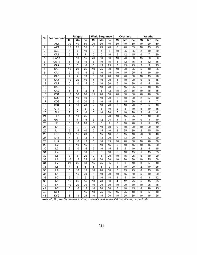
Mi Mo Se Mi Mo Se Mi Mo Se Mi Mo Se1 AL1 30 40 60 20 30 40 30 40 60 10 20 302 AZ1 15 25 35 5 23 40 6 20 35 10 15 253 AZ2 5 7 19 2 4 6 10 25 35 2 10 304 CA1 5 7 7 0 0 10 5 12 15 0 7 205 CA10 5 10 15 40 60 80 10 20 30 15 30 506 CA11 8 12 15 5 10 15 8 12 16 8 12 167 CA2 0 5 10 5 15 25 5 15 25 2 5 158 CA3 10 20 25 10 25 60 10 20 25 5 10 259 CA4 5 10 15 5 10 15 10 15 25 5 10 1010 CA5 4 7 13 3 10 20 10 20 30 10 15 2811 CA6 10 20 40 5 10 20 5 10 20 0 5 1512 CA7 5 10 15 5 10 30 5 10 20 0 5 1013 CA8 2 3 5 5 10 20 5 15 25 5 10 1514 CA9 5 8 12 5 8 12 15 25 35 10 15 1515 CO1 15 30 80 15 20 50 20 30 60 20 40 5016 CO2 4 10 40 2 10 20 2 10 20 2 5 1017 CO3 5 10 20 5 10 15 2 15 30 0 3 718 CO4 4 10 40 2 10 20 2 10 20 2 5 1019 CT1 1 2 5 2 5 10 2 5 10 5 10 1520 FL1 2 5 10 5 10 20 5 10 20 2 4 621 FL2 4 10 25 5 9 20 10 15 25 7 10 2022 GA1 4 7 15 5 12 24 1 4 10 0 3 1023 HI1 5 10 20 3 6 9 5 10 20 1 5 1524 ID1 0 0 0 20 40 60 0 10 20 10 20 4025 IL1 2 14 40 5 15 40 3 25 80 2 15 4026 IL10 10 15 20 8 15 18 8 15 18 20 30 4027 IL11 4 8 12 7 13 20 7 13 20 7 13 2028 IL12 5 10 15 5 10 15 10 20 30 10 20 3029 IL2 5 10 15 5 10 15 5 10 15 10 15 2030 IL3 5 10 15 5 10 15 2 5 10 2 5 1531 IL4 3 5 10 3 5 10 5 10 15 5 15 3532 IL5 3 8 20 2 5 20 10 15 25 5 10 2033 IL6 10 15 25 10 20 30 10 20 30 10 25 5034 IL7 20 25 30 15 25 35 0 0 10 0 5 1035 IL8 4 6 8 3 6 9 5 10 20 2 10 2536 IL9 5 10 15 10 20 30 5 15 25 0 15 2037 IN1 6 15 30 6 10 20 10 15 50 5 10 2038 IN2 2 4 6 5 10 18 1 5 10 0 3 1239 IN3 15 25 35 10 20 30 4 12 25 5 15 2540 IN4 10 20 30 10 20 30 10 20 30 10 25 4541 IN5 5 10 15 10 20 30 5 10 15 8 20 2542 KY1 5 8 15 10 25 55 15 25 40 0 5 1043 KY2 8 14 25 10 15 20 15 25 35 10 15 25
Overtime WeatherFatigue Work SequenceNo. Respondent
Note: Mi, Mo, and Se represent minor, moderate, and severe field conditions, respectively.
214

Mi Mo Se Mi Mo Se Mi Mo Se Mi Mo Se44 MA1 10 15 20 3 8 17 5 12 25 3 8 1745 MA2 5 10 20 5 10 20 5 10 20 5 10 2046 MD1 5 10 20 3 5 10 10 20 30 5 10 2047 MD2 8 10 20 9 14 20 10 15 21 8 15 2548 MD3 3 6 9 3 6 9 3 6 9 5 7 1049 MD4 8 20 37 7 17 44 7 13 25 8 19 3250 MD5 8 10 20 9 14 20 10 15 21 8 15 2551 ME1 5 10 15 5 20 45 5 10 20 10 20 3052 MI1 15 30 40 3 10 15 15 25 35 15 20 3053 MI2 0 5 30 2 10 30 10 15 25 0 10 1554 MI3 0 10 20 5 15 33 5 10 25 0 10 2555 MI4 0 2 4 2 5 15 3 7 14 0 5 1056 MN1 1 5 10 5 15 25 1 10 15 10 10 2057 MN2 0 1 5 0 2 8 0 5 10 0 0 558 MO1 3 6 9 8 11 20 10 30 35 15 20 2559 MO2 10 20 30 5 10 15 10 20 30 10 20 3060 MO3 5 10 20 5 25 40 5 25 40 5 15 4061 MO4 10 20 30 5 10 15 10 20 30 10 20 3062 MO5 2 4 10 4 9 15 3 7 10 3 10 1563 MT1 5 15 20 10 15 30 5 10 15 5 10 1564 NC1 5 8 15 2 10 20 2 5 20 5 10 2065 NC2 3 8 12 6 14 26 3 8 12 5 12 2066 ND1 1 2 4 3 5 10 1 5 15 0 2 567 NH1 5 15 20 5 10 15 0 5 15 5 10 1568 NJ1 0 5 10 0 5 10 5 10 20 5 10 2069 NV1 0 0 0 10 30 60 2 15 25 2 25 4070 NY1 0 5 10 10 20 45 5 10 15 15 25 5071 NY2 3 8 15 3 8 15 5 10 15 5 15 3072 NY3 10 20 30 15 25 50 10 20 40 15 25 5073 NY4 12 18 24 10 15 20 15 20 25 15 20 2574 NY5 3 10 20 2 7 15 2 7 15 3 10 2075 OH1 2 5 9 3 5 9 3 6 9 3 6 1276 OH2 5 10 30 20 35 70 20 40 60 20 45 8577 OH3 0 15 25 5 15 30 0 5 20 0 5 1578 OH4 10 25 50 15 30 45 10 25 50 5 50 8079 OH5 2 6 10 2 6 10 5 10 15 5 10 1580 OH6 2 5 7 2 5 7 2 5 8 3 7 1081 OH7 4 6 8 6 9 12 8 12 18 10 15 2082 OH8 1 5 12 1 4 10 0 15 30 2 15 1683 OH9 2 5 10 4 8 16 4 10 18 5 10 1584 OR1 10 20 40 5 18 35 5 20 35 10 40 10085 OR2 5 10 15 0 5 5 0 5 10 15 20 37.586 OR3 5 15 23 10 15 20 5 15 23 10 15 25
Overtime WeatherFatigue Work SequenceNo. Respondent
Note: Mi, Mo, and Se represent minor, moderate, and severe field conditions, respectively.
215

Mi Mo Se Mi Mo Se Mi Mo Se Mi Mo Se87 PA1 5 8 15 5 12 25 5 15 25 3 11 1588 PA2 5 15 25 10 25 50 10 25 50 5 10 2089 PA3 5 30 35 10 40 60 5 10 15 15 50 7590 PA4 5 15 20 10 20 35 5 10 15 10 15 2091 PA5 15 30 50 10 20 40 0 10 25 0 10 3092 SC1 15 30 60 15 30 60 20 30 40 15 30 4593 SC2 20 30 40 10 20 35 10 20 40 5 10 1594 SC3 10 20 30 4 20 30 8 22 40 3 10 2095 TN1 5 10 20 5 10 20 5 10 20 5 10 2096 TN2 5 13.5 25 5 21 35 5 15 30 7.5 22.5 5097 TN3 5 13 20 6 15 22 7 17 27 7 16 2798 TX1 7 21 35 5 15 30 15 25 35 5 15 2599 TX10 8 24 40 8 24 40 8 24 40 5 15 25100 TX11 15 25 35 10 20 30 15 30 45 15 30 45101 TX12 10 30 50 10 25 30 20 33 50 15 20 40102 TX2 10 20 30 12 16 32 10 20 30 10 20 30103 TX3 10 25 35 15 35 45 10 25 40 8 15 25104 TX4 8 14 22 12 20 30 15 25 40 12 19 26105 TX5 10 20 30 10 30 40 15 30 50 10 25 40106 TX6 10 20 25 5 15 35 10 25 50 5 15 30107 TX7 2 10 20 10 20 30 2 10 20 2 10 15108 TX8 20 60 100 5 20 40 0 10 30 10 15 40109 TX9 4 9 20 15 35 60 12 30 50 3 8 15110 UT1 5 15 30 5 10 15 5 12 25 5 15 30111 VA1 5 10 15 15 30 45 5 10 15 5 10 20112 VA2 5 10 15 10 15 20 10 20 35 20 30 40113 VA3 3 8 10 5 8 12 3 6 9 2 7 10114 VA4 20 40 80 5 15 50 20 50 80 1 3 10115 VA5 15 35 45 15 35 40 15 35 45 15 25 35116 VA6 5 5 5 10 15 25 10 20 25 10 10 15117 VA7 2 5 20 2 10 20 10 15 20 10 25 40118 VT1 3 7 15 3 10 15 5 15 20 5 10 15119 WA1 10 20 30 10 25 50 10 15 20 3 8 17120 WA2 2 5 10 2 5 10 5 15 30 5 10 20121 WA3 2 15 25 2 10 20 5 15 20 2 10 20122 WI1 3 6 12 3 6 12 4 8 16 4 8 16123 WI2 2 6 10 2 6 10 3 8 13 10 25 60124 WI3 2 3 4 1 3 5 1 2 3 1 4 15125 WI4 20 40 67.5 15 25 40 15 30 50 15 25 50126 WI5 10 20 40 10 20 40 10 10 30 20 40 60127 WI6 3 5 8 5 8 10 5 10 12 2 5 8128 WV1 2 5 8 5 8 10 4 8 12 0 2 2129 WY1 10 15 25 10 15 25 10 20 25 10 20 25
Overtime WeatherFatigue Work SequenceNo. Respondent
Note: Mi, Mo, and Se represent minor, moderate, and severe field conditions, respectively.
216

Appendix D Summary of Significant Facts of the Validation Projects
217

Project 1: Parking Garage
• A total masonry cost of approximately $1,000,000
• Completed within budget and on-time
• Below-average change orders and average rework requested by the owner
• Similar design as a previous project
• Not enough skilled personnel with high absence of the masonry workers
• Worked with plumbing and electrical workers in the same area at least
once a week (congestion)
• Difficult to access brick storage due to other trades working around that
area (site access)
• Crew composition: 10 bricklayers, 15 bricklayer helpers, 2 forklift
operators, and 1 superintendent
Project 2: Office Building
• A total masonry cost of approximately $1,000,000
• Ongoing work and likely to be on-time and within budget
• Below-average change orders and average rework requested by the owner
• Redesigned with an amendment at short notice
• Partially occupied for an adjoining building (joint occupancy)
• Encountered change orders resulting in change in work sequence (work
sequence)
218

Project 2: Office Building (Cont’d)
• Crew composition: 10 bricklayers, 15 bricklayer helpers, 2 forklift
operators, and 1 superintendent
Project 3: Parking Garage
• A total masonry cost of approximately $1,100,000
• Completed within budget and on-time
• Average change orders and below-average rework requested by the owner
• Obtained addenda with significant change in design
• Other trades working in the same area at least once a week (congestion)
• Crew composition: 10 bricklayers, 15 bricklayer helpers, 2 forklift
operators, and 1 superintendent
Project 4: School Building
• A total masonry cost of approximately $3,000,000
• Ongoing work and likely to be over-budget and delayed
• Above-average change orders and rework requested by the owner
• Complex masonry work, large amount of detail
• Incomplete and poor set of document and drawings (errors and omissions)
• Lack of answers to RFI’s (diverted supervision)
219

Project 4: School Building (Cont’d)
• Experienced owner’s negative attitude toward the masonry contract
(morale and attitude)
• Crew composition: 14 bricklayers, 14 bricklayer helpers, 4 machine
operators, and 3 superintendents
Project 5: Student Dormitory
• A total masonry cost of approximately $2,600,000
• Completed within budget, but delayed
• Below-average change orders and average rework requested by the owner
• Under-cover working condition
• Worked with steel and plumbing workers in the same area (congestion)
• Crew composition: 14 bricklayers and 16 bricklayer helpers
220

Appendix E Summary of Distributed and Returned Questionnaires
221

No. State Questionnaires Distributed
Questionnaires Responded
Total Reponses
(%)
Valid Responses
Valid Responses
(%)(a) (b) (b)/(a) x 100 (c) (c)/(b) x 100
1 AL 7 1 14% 1 100%2 AR 1 0 0% 0 -3 AZ 9 2 22% 2 100%4 CA 187 15 8% 11 73%5 CO 18 5 28% 4 80%6 CT 12 1 8% 1 100%7 DE 2 0 0% 0 -8 FL 13 3 23% 2 67%9 GA 9 1 11% 1 100%
10 HI 1 1 100% 1 100%11 IA 6 1 17% 0 0%12 ID 1 1 100% 1 100%13 IL 123 14 11% 12 86%14 IN 22 5 23% 5 100%15 KS 4 0 0% 0 -16 KY 15 3 20% 2 67%17 LA 2 1 50% 0 0%18 MA 6 3 50% 2 67%19 MD 17 5 29% 5 100%20 ME 2 1 50% 1 100%21 MI 29 6 21% 4 67%22 MN 11 2 18% 2 100%23 MO 76 6 8% 5 83%24 MS 3 0 0% 0 -25 MT 3 1 33% 1 100%26 NC 19 2 11% 2 100%27 ND 1 0 0% 0 -28 NE 5 2 40% 1 50%29 NH 3 1 33% 1 100%30 NJ 4 1 25% 1 100%31 NM 1 0 0% 0 -32 NV 11 1 9% 1 100%33 NY 14 5 36% 5 100%34 OH 76 9 12% 9 100%35 OK 1 0 0% 0 -36 OR 12 3 25% 3 100%37 PA 25 7 28% 5 71%38 SC 6 3 50% 3 100%39 SD 1 0 0% 0 -40 TN 12 3 25% 3 100%41 TX 92 15 16% 12 80%42 UT 5 2 40% 1 50%43 VA 21 7 33% 7 100%44 VT 5 1 20% 1 100%45 WA 26 3 12% 3 100%46 WI 27 7 26% 6 86%47 WV 1 1 100% 1 100%48 WY 3 1 33% 1 100%
TOTAL 950 152 16% 129 85%
222

Appendix F Summary of Data Analyses Results
223

Summary of Analysis Results from the Model Development Process AFTER Eliminating Outliers
StatisticsMinor Moderate Severe Minor Moderate Severe Minor Moderate Severe
N Valid 112 110 114 94 113 112 112 113 113Missing 4 6 2 22 3 4 4 3
Mean 5 12 24 4 12 21 5 12 21Std. Error of Mean 0.27 0.55 1.12 0.21 0.70 1.13 0.30 0.60 1.07Median 5 10 20 5 10 20 5 10 20Mode 5 10 20 5 10 20 5 10 20Std. Deviation 2.91 5.79 11.92 2.03 7.40 11.93 3.14 6.35 11.411.96 x (SE) 0.54 1.08 2.19 0.41 1.36 2.21 0.58 1.17 2.10Mean-1.96x(SE) 4.57 11.18 22.28 3.31 10.81 18.53 4.11 10.52 19.38Mean+1.96x(SE) 5.65 13.34 26.65 4.13 13.54 22.95 5.27 12.86 23.59Variance 8.47 33.49 142.11 4.13 54.71 142.21 9.84 40.38 130.09Skewness 0.45 0.56 0.87 -0.29 0.81 0.70 0.67 0.76 0.87Std. Error of Skewness 0.23 0.23 0.23 0.25 0.23 0.23 0.23 0.23 0.23Kurtosis -0.62 -0.39 0.04 -0.29 0.02 0.03 0.03 -0.34 0.21Std. Error of Kurtosis 0.45 0.46 0.45 0.49 0.45 0.45 0.45 0.45 0.45Range 10 23 45 9 30 55 15 28 48Minimum 0 2 5 0 0 0 0 2 2Maximum 10 25 50 9 30 55 15 30 50Sum 572.5 1348.5 2789 349.5 1376 2323 525 1321 2428Percentiles 10 2 5 10 0 5 8 1 5
25 3 8 15 2 7 12 2 6.5 1250 5 10 20 5 10 20 5 10 2075 6 15 30 5 15 30 5.75 15 3090 10 20 50 5 25 40 10 20 40
StatisticsMinor Moderate Severe Minor Moderate Severe Minor Moderate Severe
N Valid 115 110 113 95 112 108 115 114 112Missing 1 6 3 21 4 8 1 2
Mean 5 11 20 4 11 18 6 13 22Std. Error of Mean 0.34 0.50 1.00 0.19 0.51 0.80 0.32 0.66 1.22Median 5 10 20 5 10 16 5 10 20Mode 5 10 20 5 10 20 5 10 15Std. Deviation 3.61 5.26 10.66 1.89 5.35 8.29 3.40 7.07 12.881.96 x (SE) 0.66 0.98 1.97 0.38 0.99 1.56 0.62 1.30 2.38Mean-1.96x(SE) 4.47 9.67 18.02 3.37 9.57 16.54 4.93 11.34 20.00Mean+1.96x(SE) 5.80 11.64 21.96 4.13 11.55 19.66 6.17 13.93 24.77Variance 13.06 27.71 113.74 3.56 28.63 68.65 11.56 50.00 165.79Skewness 0.62 0.84 1.01 -0.08 0.91 0.71 0.65 0.80 0.91Std. Error of Skewness 0.23 0.23 0.23 0.25 0.23 0.23 0.23 0.23 0.23Kurtosis -0.16 0.14 0.89 0.37 0.41 0.20 0.01 -0.12 -0.10Std. Error of Kurtosis 0.45 0.46 0.45 0.49 0.45 0.46 0.45 0.45 0.45Range 15 22 45 10 23 36 15 28Minimum 0 3 5 0 2 4 0 2 5Maximum 15 25 50 10 25 40 15 30Sum 590.5 1172 2259 356 1183 1955 638.5 1440.5 2507Percentiles 10 0 5 8 1 5 9 2 5 9
25 2 6.75 11 2 6 11.25 3 8 1250 5 10 20 5 10 15.5 5 10 2075 8 15 25 5 15 24.75 8 18 3090 10 20 33 5 20 30 10 25 45
Added Operations Diverted Supervision
Congestion Morale and Attitude Labor Reassignment
Crew Size Change
3
10
4
50
55
224

StatisticsMinor Moderate Severe Minor Moderate Severe Minor Moderate Severe
N Valid 98 114 110 97 114 110 116 115 114Missing 18 2 6 19 2 6 0 1 2
Mean 4 11 18 4 11 19 7 14 25Std. Error of Mean 0.21 0.57 0.96 0.19 0.55 0.91 0.51 0.83 1.32Median 5 10 15 5 10 15 5 10 20Mode 5 10 15 5 10 15 10 10 15Std. Deviation 2.04 6.13 10.10 1.88 5.84 9.57 5.50 8.93 14.141.96 x (SE) 0.40 1.13 1.89 0.37 1.07 1.79 1.00 1.63 2.59Mean-1.96x(SE) 3.59 9.87 16.18 3.42 9.67 16.94 5.64 11.91 22.15Mean+1.96x(SE) 4.39 12.12 19.96 4.17 11.82 20.52 7.64 15.17 27.34Variance 4.18 37.63 101.97 3.54 34.16 91.65 30.20 79.76 199.80Skewness 0.06 0.80 0.99 -0.48 0.86 0.86 0.93 0.86 0.84Std. Error of Skewness 0.24 0.23 0.23 0.24 0.23 0.23 0.22 0.23 0.23Kurtosis -0.20 -0.25 0.45 -0.50 0.26 0.14 0.05 0.27 0.01Std. Error of Kurtosis 0.48 0.45 0.46 0.49 0.45 0.46 0.45 0.45 0.45Range 9 23 46 8 23 41 20 40 61.5Minimum 0 2 4 0 2 4 0 0 1Maximum 9 25 50 8 25 45 20 40 63Sum 391 1253.5 1987.5 368 1225 2060 770.5 1557 2820.5Percentiles 10 1 4.5 6.2 1 5 8.1 1 5 10
25 2 6 10 2.5 5 10 2 6 1550 5 10 15 5 10 15 5 10 2075 5 15 20.25 5 15 25 10 20 31.2590 6.1 20 35 5 20 34.5 15 25 50
StatisticsMinor Moderate Severe Minor Moderate Severe Minor Moderate Severe
N Valid 116 116 114 111 112 116 108 111 116Missing 0 0 2 5 4 0 8 5 0
Mean 7 14 25 7 14 27 7 15 26Std. Error of Mean 0.41 0.66 1.06 0.41 0.68 1.20 0.35 0.67 1.30Median 5 15 25 5 15 25 6 15 25Mode 10 15 20 5 10 20 10 10 20Std. Deviation 4.43 7.09 11.27 4.28 7.24 12.96 3.62 7.10 14.021.96 x (SE) 0.81 1.29 2.07 0.80 1.34 2.36 0.68 1.32 2.55Mean-1.96x(SE) 6.02 12.69 23.14 6.12 12.73 24.33 6.32 13.35 23.93Mean+1.96x(SE) 7.63 15.27 27.28 7.71 15.41 29.05 7.69 15.99 29.03Variance 19.62 50.26 127.07 18.34 52.47 167.83 13.08 50.44 196.58Skewness 0.66 0.57 0.44 0.41 0.33 0.40 0.27 0.45 0.78Std. Error of Skewness 0.22 0.22 0.23 0.23 0.23 0.22 0.23 0.23 0.22Kurtosis 0.01 0.22 -0.32 -0.52 -0.60 -0.52 -0.50 -0.26 0.66Std. Error of Kurtosis 0.45 0.45 0.45 0.46 0.45 0.45 0.46 0.46 0.45Range 20 35 46 15 30 60 15 32.5 7Minimum 0 0 4 0 0 0 0 0 0Maximum 20 35 50 15 30 60 15 33Sum 792 1621.5 2873.5 767.5 1575.5 3096 756.5 1628.5 3071.5Percentiles 10 2 5 10 2 5 10 2 6
25 3 9.25 19.5 5 10 16.25 5 10 15.2550 5 15 25 5 15 25 6 15 2575 10 20 30.75 10 20 35 10 20 3590 12.9 22.9 40 15 25 46.5 10 25 45
Beneficial Occupancy
Joint Occupancy Site Access Logistics
Learning Curve Errors and Omissions
2.5
73
10
225

StatisticsMinor Moderate Severe Minor Moderate Severe Minor Moderate Severe
N Valid 112 111 114 116 116 113 115 115 114Missing 4 5 2 0 0 3 1 1 2
Mean 5 11 20 6 14 23 7 15 24Std. Error of Mean 0.35 0.59 1.00 0.36 0.70 1.10 0.39 0.69 1.06Median 5 10 20 5 10 20 5 15 22Mode 5 10 20 5 10 20 5 10 20Std. Deviation 3.70 6.25 10.63 3.84 7.51 11.74 4.16 7.36 11.311.96 x (SE) 0.68 1.16 1.95 0.70 1.37 2.16 0.76 1.35 2.08Mean-1.96x(SE) 4.64 10.08 18.04 5.41 12.23 20.99 5.87 13.38 22.39Mean+1.96x(SE) 6.01 12.40 21.94 6.81 14.96 25.31 7.39 16.07 26.54Variance 13.66 39.05 113.09 14.73 56.36 137.81 17.32 54.24 127.91Skewness 0.82 0.66 0.61 0.74 0.86 0.63 0.45 0.47 0.64Std. Error of Skewness 0.23 0.23 0.23 0.22 0.22 0.23 0.23 0.23 0.23Kurtosis 0.23 -0.49 -0.37 -0.12 0.38 -0.51 -0.58 -0.46 -0.25Std. Error of Kurtosis 0.45 0.46 0.45 0.45 0.45 0.45 0.45 0.45 0.45Range 15 24 46 15 35 45 15 35Minimum 0 1 4 0 0 5 0 0 3Maximum 15 25 50 15 35 50 15 35Sum 596 1247.5 2279 709 1577 2616 762 1693 2789Percentiles 10 1 5 8 2 5 10 1.6 5 10
25 2.25 6 10 3 8.25 15 4 10 1550 5 10 20 5 10 20 5 15 2275 8 15 26.25 10 20 30 10 20 3090 10 20 36 10 25 40 13.2 25 40
StatisticsMinor Moderate Severe
N Valid 116 111 113Missing 0 5 3
Mean 6 12 22Std. Error of Mean 0.43 0.59 1.02Median 5 10 20Mode 5 10 20Std. Deviation 4.65 6.25 10.881.96 x (SE) 0.85 1.16 2.01Mean-1.96x(SE) 5.17 11.13 20.11Mean+1.96x(SE) 6.86 13.46 24.13Variance 21.64 39.12 118.47Skewness 0.77 0.43 0.85Std. Error of Skewness 0.22 0.23 0.23Kurtosis 0.22 -0.50 0.39Std. Error of Kurtosis 0.45 0.46 0.45Range 20 25 48Minimum 0 0 2Maximum 20 25 50Sum 697.5 1364.5 2499.5Percentiles 10 0 5 10
25 2 8 1550 5 10 2075 10 15 27.590 12.9 20 40
Fatigue Work Sequence Overtime
Weather or Environment
47
50
226

Summary of Analysis Results from the Model Development Process BEFORE Eliminating Outliers
No. Field Factors
Estimated Percentage of Productivity Loss (%),
If the Factor Is … (0% to 100% in each column)
Minor Moderate Severe 1 Congestion 6
0-25 13
2-35 26
5-65
2 Morale and Attitude 5 0-28
13 0-35
22 0-70
3 Labor Reassignment 5 0-15
12 2-40
22 2-65
4 Crew Size Change 5 0-25
12 3-50
21 5-80
5 Added Operations 5 0-20
12 2-50
22 4-70
6 Diverted Supervision: 6 0-30
13 2-40
25 5-75
7 Learning Curve 5 0-20
12 2-35
20 4-70
8 Errors and Omissions 5 0-15
11 2-40
21 4-75
9 Beneficial Occupancy 7 0-20
14 0-45
26 1-75
10 Joint Occupancy 7 0-20
14 0-35
26 4-70
11 Site Access 8 0-25
15 0-40
28 0-75
12 Logistics 8 0-20
16 0-40
27 0-72
13 Fatigue 6 0-20
12 1-40
21 4-80
14 Work Sequence 6 0-20
14 0-35
25 5-70
15 Overtime 7 0-20
15 0-50
26 3-80
16 Weather or Environment 6 0-20
13 0-50
24 2-100
Note: This table presents low, mean, and high percentages of productivity loss from the raw
data.
227

Summary of Analysis Results from the Model Validation Process
Statistics PROJECT1 PROJECT2 PROJECT3 PROJECT4 PROJECT5N Valid 114 116 110 114 112
Missing 2 0 6 2 4Mean 10.60 27.57 12.26 38.18 5.11Std. Error of Mean 0.58 1.17 0.55 1.71 0.27Median 10 25 10 35 5Mode 10 20 10 35 5Std. Deviation 6.23 12.60 5.79 18.30 2.911.96 x (SE) 1.14 2.29 1.08 3.36 0.54Mean-1.96x(SE) 9.5 25.3 11.2 34.8 4.6Mean+1.96x(SE) 11.7 29.9 13.3 41.5 5.7Variance 38.77 158.69 33.49 334.96 8.47Skewness 0.59 0.41 0.56 0.70 0.45Std. Error of Skewness 0.23 0.22 0.23 0.23 0.23Range 28 50 23 85 10Minimum 0 5 2 5 0Maximum 28 55 25 90 1Sum 1208 3198.5 1348.5 4352 572.5Percentiles 10 3 13 5 18 2
25 6 16.25 8 23.75 350 10 25 10 35 575 15 36 15 50 690 20 45 20 65 10
0
228

BIBLIOGRAPHY Agresti, A. and Finlay, B. (1997). Statistical Methods for the Social Sciences. Prentice Hall, Upper Saddle River, New Jersey. Allmon, E., Haas, C. T., Borcherding, J. D., and Goodrum, P. M. (2000). “U.S. Construction Labor Productivity Trends, 1970-1998.” Journal of Construction Engineering and Management, ASCE, 126(2), 97-104. American Subcontractors Association (1979). “Owner’s Guide On Overtime, Construction Costs and Productivity.” American Subcontractors Association, The Associated General Contractors of America and the Associated Specialty Contractors, Inc. The Army of Corps of Engineers (1979). Modification Impact Evaluation Guide. Office of the Chief of Engineers, Department of Army, Washington, DC 20314, July. Borcherding J. D. (1976). “Improving Productivity in Industrial Construction.” Journal of the Construction Division, ASCE, 102(CO4), 599-614. Borcherding, J. D., and Alarcon, L. F. (1991). “Quantitative Effects on Construction Productivity.” The Construction Lawyer, American Bar Association, 11(1), 35-48. Borcherding J. D. and Garner, D. F. (1981). “Work Force Motivation and Productivity on Large Projects.” Journal of the Construction Division, ASCE, 107(CO3), 443-453. Borcherding J. D. and Oglesby C. H. (1974). “Construction Productivity and Job Satisfaction.” Journal of the Construction Division, ASCE, 100(CO3), 413-431. Borcherding J. D., Sebastian, S. J., and Samelson, N. M. (1980). “Improving Motivation and Productivity on Large Projects.” Journal of the Construction Division, ASCE, 106(CO1), 73-89. The Business Roundtable (1982). “Construction Labor Motivation.” Construction Industry Cost Effectiveness Task Force Report, August. The Business Roundtable (1982). “Absenteeism and Turnover.” Report C6, June.
229

The Business Roundtable (1980). “Scheduled Overtime Effect on Construction Projects.” Construction Industry Cost Effectiveness Task Force Report, November. Bureau of Engineering Research (1991). “Managing Subcontractor Safety.” Publications 13-1, Construction Industry Institute (CII), The University of Texas at Austin. Bureau of Engineering Research (1986a). “Constructability – A Primer.” Publications 3-1, Construction Industry Institute (CII), The University of Texas at Austin. Bureau of Engineering Research (1986b). “Impact of Various Construction Contract Types and Clauses on Project Performance.” Publications 5-1, Construction Industry Institute (CII), The University of Texas at Austin. Cho, S. (2000). “Development of the Project Definition Rating Index (PDRI) for Building Projects.” Doctoral Dissertation, The University of Texas at Austin, Austin, TX, May 2000. Construction Industry Institute (2000). “Quantifying the Cumulative Impact of Change Orders for Electrical and Mechanical Contractors.” Research Summary 158-1, Cumulative Change Order Impact Research Team, Construction Industry Institute (CII), The University of Texas at Austin. Construction Industry Institute (1988). “The Effect of Schedule Overtime Shift Schedule on Construction Craft Productivity.” Source Document 43, Productivity Measurements Task Force Overtime and Shiftwork Subcommittee, Construction Industry Institute (CII), The University of Texas at Austin. Cooper, R. A. and Weekes, A. J. (1983). Data, Models and Statistical Analysis. Barnes and Noble Books, Totowa, New Jersey. Dieterle, R., and DeStephanis, A. (1992). “Use of Productivity Factors in Construction Claims.” Transactions of American Association of Cost Engineers, AACE, 1, C.1.1-C.1.7. Edmonson, C. H. (1974). “You can Predict Construction Labor Productivity.” Hydrocarbon Processing, July, 167-180. Fotheringam, A. S, Brunsdon, C., and Charlton, M. (2000). Quantitative Geography: Perspectives on Spatial Data Analysis. SAGE Publications Ltd., London.
230

Fowler, F. J. (1993). Survey Research Methods, 2nd Edition, SAGE Publications, Inc., Newbury Park, CA. Gibson, G. E. and Hamilton (1994). “Analysis of Pre-Project Planning Effort and Success Variables for Capital Facility Projects.” Source Document 105, Construction Industry Institute (CII), The University of Texas at Austin. Gibson, G. E., Kaczmarowski, J. H., and Lore, H. E. (1993). “Modeling Pre-Project Planning for the Construction of Capital Facilities.” Source Document 94, Construction Industry Institute (CII), The University of Texas at Austin. Goodrum, P. M. (2001). “The Impact of Equipment Technology on Productivity in the U.S. Construction Industry.” Doctoral Dissertation, The University of Texas at Austin, Austin, TX, May 2001. Griffith, A. F. and Gibson, G. E. (1997). “Team Alignment During Pre-project Planning of Capital Facilities.” Research Reports 133-12, Construction Industry Institute (CII), The University of Texas at Austin. Grimm, C. T. (1974). “Masonry Construction Operations.” Journal of the Construction Division, ASCE, 100(CO2), 171-185. Grimm, C. T. and Wagner, N. K. (1974). “Weather Effects on Mason Productivity.” Journal of the Construction Division, ASCE, 100(CO3), 319-335. Handa, V. K. and Rivers, D. (1983). “Downgrading Construction Incidents.” Journal of Construction Engineering and Management, ASCE, 109(2), 190-205. Heather P. R. and Summers, M. D. (1996). “Consequential Cost Effects.” Transactions of the American Association of Cost Engineers, AACE, C&C.7.1-C&C.7.7. Hester, W. T., Kuprenas, J. A. and Chang, T. C. (1991). “Construction Changes and Change Orders: Their Magnitude and Impact.” Source Document 66, Construction Industry Institute (CII), The University of Texas at Austin. Howenstine, E. J. (1975). “Productivity Trends in the Construction Industry: A Comparative International Review.” Bulletin 17, American Association of Cost Engineers, 73(6), 189-194.
231

Kerlinger, F. N. and Pedhazur, E. J. (1973). Multiple Regression in Behavioral Research. Holt, Rinehart and Winston, Inc., New York, NY. Koehn, E. and Brown, G. (1985). “Climatic Effects on Construction.” Journal of Construction Engineering and Management, ASCE, 111(2), 129-137. Koehn, E. and Caplan, S. B. (1987). “Work Improvement Data for Small and Medium Size Contractors.” Journal of Construction Engineering and Management, ASCE, 113(2), 327-339. Koehn, E. and Manuel, J. (1988). “Variation in Work Improvement Potential for Small/medium Contractors.” Journal of Construction Engineering and Management, ASCE, 114(3), 505-509. Laufer, A. and Borcherding, J. D. (1981). “Using Pay to Motivate Construction Workers’ Performance.” Transactions of the American Association of Cost Engineers, AACE, I.6.1-I.6.4. Leonard, C. A. (1987). “The Effect of Change Orders on Productivity.” The Revay Report, On-line. World Wide Web. February 14, 2000. Available URL: http://www.revay.com/articles/V6N2ALL.html Leonard, C. A., Fazio, P. and Moselhi, O. (1988). “Construction Productivity: Major Causes of Impact.” Transactions of the American Association of Cost Engineers, AACE, D.10.1-D.10.7. Mechanical Contractors of America (1976). “Factors Affecting Productivity.” Mechanical Contractors of America, Bulletin No. 58, January. National Electrical Contractors Association (1989). “Overtime and Productivity in Electrical Construction.” NECA, 2nd Edition, Washington, DC. Neil, J. M. and Knack, L. E. (1984). “Predicting Productivity.” Transactions of American Association of Cost Engineers, AACE, H.3.1-H.3.8. Oglesby, C. H., Parker, H. W. and Howell, G. A. (1989). Productivity Improvement in Construction. McGraw-Hill, Inc., New York, N.Y. Ovararin, N., and Popescu, C. M. (2001). “Field Factors Affecting Masonry Productivity.” The 45th Annual Meeting of AACE International, Association for the Advancement of Cost Engineering, June 17-20, 2001.
232

Parker, H. and Oglesby, C. (1972). Methods Improvement for Construction Managers, McGraw-Hill, Inc., New York, N.Y. Revay, S. G. (1984). “An Improved Technique of Productivity Measurements.” Transactions of the American Association of Cost Engineers, AACE, H.1.1-H.1.5. Revay, S. G. (1991). “Quantifying Construction Claims!” The Revay Report, On-line. World Wide Web. February 14, 2000. Available URL: http://www.revay.com/articles/V10N1ALL.html R.S. Means Company, Inc. (2000). R.S. Means Building Construction Cost Data, 59th Annual Edition, R.S. Means Company, Inc., Kingston, MA, p. 127, 538. Sanders, S. R. and Thomas, H. R. (1993). “Masonry Productivity Forecasting Model.” Journal of Construction Engineering and Management, ASCE, 119(1), 163-179. Sanders, R. S. and Thomas H. R. (1991). “Factors Affecting Masonry-Productivity.” Journal of Construction Engineering and Management, ASCE, 117(4), 626-644. Schwartzkopf, William (1995). Calculating Lost Labor Productivity in Construction Claims. John Wiley and Sons, Inc. New York. N.Y. SPSS Inc. (1990). SPSS Introductory Statistics Student Guide, SPSS Inc., Chicago, IL. Stall, M. D. (1983). “Analyzing and Improving Productivity with Computerized Questionnaires and Delay Surveys.” Proceedings of the Project Management Institute Annual Seminar Symposium 1983, Project Management Institution, Drexel Hill, P.A., V.M.1-V.M.11. Tatum, C. B., Vanegas, J. A. and Williams, J. M. (1986). “Constructability Improvement During Conceptual Planning.” Source document 4, Construction Industry Institute (CII), The University of Texas at Austin. Thomas, H. R. (1992). “Effects of Scheduled Overtime on Labor Productivity.” Journal of Construction Engineering and Management, ASCE, 118(1), 60-76.
233

Thomas, H. R. (1990). “Effects of Scheduled Overtime on Labor Productivity: A Literature Review and Analysis.” Source Document 60, Construction Industry Institute (CII), The University of Texas at Austin. Thomas, H. R. and Kramer, D. F. (1988). “The Manual of Construction Productivity Measurement and Performance Evaluation.” Source Document 35, Construction Industry Institute (CII), The University of Texas at Austin. Thomas H. R., Maloney W. F., Horner R.M.W., Smith G. R., Handa, V. K. and Sanders S. R. (1990). “Modeling Construction Labor Productivity.” Journal of Construction Engineering and Management, ASCE, 116(4), 705-726. Thomas, H. R. and Mathews, C. T. (1986). “An Analysis of the Methods of for Measuring Construction Productivity.” Source Document 13, Construction Industry Institute (CII), The University of Texas at Austin. Thomas, H. R., Mathews, C. T. and Ward, J. G. (1986). “Learning Curve Models of Construction Productivity.” Journal of Construction Engineering and Management, ASCE, 112(2), 245-258. Thomas H. R. and Napolitan, C. L. (1994). “The Effects of Changes on Labor Productivity: Why and How Much.” Source Document 99, Construction Industry Institute (CII), The University of Texas at Austin. Thomas, H. R., and Oloufa A. A. (1995). “Labor Productivity, Disruptions, and The Ripple Effect.” Cost Engineering, 37(12), 49-54. Thomas, H. R. and Raynar, K. A. (1994). “Effects of Scheduled Overtime on Labor Productivity: A Quantitative Analysis.” Source Document 98, Construction Industry Institute (CII), The University of Texas at Austin. Thomas, H. R. and Raynar, K. A. (1997). “Schedule Overtime and Labor Productivity: Quantitative Analysis.” Journal of Construction Engineering and Management, ASCE, 123(2), 181-188. Thomas, H. R., Riley, D. R. and Sanvido, V. E. (1999). “Loss of Labor Productivity Due to Delivery Methods and Weather.” Journal of Construction Engineering and Management, ASCE, 125(1), 39-46.
234

Thomas, H. R. and Sakarcan, A. S. (1994). “Forecasting Labor Productivity Using Factor Model.” Journal of Construction Engineering and Management, ASCE, 120(1), 228-239. Thomas, H. R., Sanvido, V. E., and Sanders, S. R. (1989). “Impact of Material Management on Productivity- A Case Study.” Journal of Construction Engineering and Management, ASCE, 115(3), 370-384. Thomas, H. R. and Smith, G. R. (1990). “Loss of Construction Labor Productivity Due to Inefficiencies and Disruption: The Weight of Expert Opinion”, 163, December. Thomas, H. R. and Yiakoumis, I. (1987). “Factor Model of Construction Productivity.” Journal of Construction Engineering and Management, ASCE, 113(4), 623-639. Thomas, H. R. and Završki, I. (1999). “Construction Baseline Productivity: Theory and Practice.” Journal of Construction Engineering and Management, ASCE, 125(5), 295-303. Thomas, S. R. (1996). “An Assessment Tool for Improving Project Team Communications.” Doctoral Dissertation, The University of Texas at Austin, Austin, TX, December 1996. Thomas, S. R., Tucker, R. L. and Kelly, W. R. (1998). “Critical Communications Variables.” Journal of Construction Engineering and Management, ASCE, 124(1), 58-66. Tucker, R. L., Kelly, W. R. and Thomas, S. R. (1997). “An Assessment Tool for Improving Project Team Communications.” Research Reports 105, Construction Industry Institute (CII), The University of Texas at Austin. Tuekey, J. (1977). Exploratory Data Analysis. Addison-Wesley, Reading, MA. United Nations Committee on Housing, Building and Planning (1965). Effect of Repetition on building operations and Processes on Site. United Nations, New York, NY. United States Department of Labor, Bureau of Labor Statistics, News, August 17, 2000, http://stats.bls.gov/special.requests/ocwc/oshwc/cfoi/cfnr0006.pdf, April 26, 2001.
235
Wonnacott, T. H. and Wannacott, R. J. (1984). Introductory Statistics for Business and Economics. John Wiley & Sons, Inc., U.S. Zeitoum, A. A. and Oberlender, G. D. (1993). “Early Warning Signs of Project Changes.” Sources Document 91, Construction Industry Institute (CII), The University of Texas at Austin.
236

VITA
Nuntapong Ovararin was born in Nakhon Si Thammarat, Thailand, on
November 8, 1971, the son of Suporn Ovararin and Suntad Ovararin. After
completing his work at Benjamarachuthit High School, Nakhon Si Thammarat,
Thailand, in 1989, he entered the Prince of Songkla University in Songkla, Thailand.
He received a Bachelor of Engineering in Civil Engineering from Prince of Songkla
University in March 1994. During the following years, he worked as a field engineer
at Unimar Engineering Co., Ltd. In August 1995, Nuntapong Ovararin continued his
studies at the University of Illinois at Urbana-Champaign. He received a Master of
Science in Civil Engineering in May 1997. Then he continued his graduate studies at
the University of Texas at Austin, pursuing the degree of Doctor of Philosophy in
Civil Engineering.
Permanent Address:
089/46 Karome Road, Posadat, Meung
Nakhon Si Thammarat 80000, Thailand
This dissertation was typed by the author.
237