AC 2007-3039: CHANGE ORDERS IMPACT ON PROJECT COST

Engy Serag, San Diego State University

Amr Oloufa, University of Central Florida

© American Society for Engineering Education, 2007

CHANGE ORDERS IMPACT ON PROJECT COST

ABSTRACT

Change orders occur frequently in most construction projects. Changes occur not only because of

errors and omissions, but also for other reasons such as scope of work changes, or changes

because of unforeseen conditions encountered on the site; a problem which is very common in

most heavy construction projects. Several studies have attempted to quantify the impact of

change orders on the project cost. Almost all of the studies in this area were sponsored by

contractors’ organizations, where statistical model used to quantify the impact of the change

orders on the project cost was based on data supplied by the contractors; a situation that lead to

owner-contractor disagreements related to the quantification method used. Also, resulting change

order models didn’t rely on the actual plans, specs, daily productivity and changes of the project;

rather they relied on the reply of the contractor filling survey.

The study addresses the need for a statistical model to quantify the increase of the contract price

due to change orders from verifiable site data such as owner’s daily reports, change orders,

drawing, and specifications. A model is developed and validated to quantify the percent increase

in the contract price due to the change orders. This model will provide the owner with an

estimate of the cost of the changed work, where it can be used for forward pricing or

retrospective pricing of the change orders

INTRODUCTION

Change orders are frequently encountered in any construction project. Contract modifications

that increase the contract value from 5 to 10% are expected in most construction projects1. The

value of construction work put in place in 2003 was $ 870 billion according to the US Census

Bureau. A 5% change rate on this $ 870 billion means that just the direct costs of change

approach $44 billion per year. In addition there are other indirect costs such as higher insurance

rates, delayed completion of projects; and lost opportunity of bidding in other projects due to

extended completion; and so forth. The major variable risk item in any construction project is the

labor as they are frequently the most variable cost for the contractor. The main areas of labor cost

increase include schedule acceleration, changes in the scope of work, project management,

project location and external characteristics2.

The main objective of the research is the following: (1) Analyze the change orders issued by the

owner and their effect on project cost. (2) Develop a model to assist the owner to quantify the

increase in the contract price resulting from change orders.

DATA PREPARATION

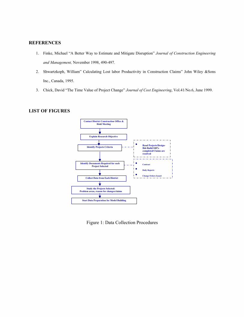
The most important step is to define the projects criteria under study; which is achieved through

running multiple interviews with several claims consultants that handled construction claims for

both the owner and the contractor. Figure 1 summarizes the data collection steps. After

collecting the data from the projects, the data is prepared to start the model building step by: (1)

determining the dependant variable; and (2) determining the predictor variables.

Dependant Variable (Response):

The main objective of this study is to quantify the percent increase in the contract price due to

change orders. It will be referred to in this study as the dependant variable.

($)

100($) . %

projecttheofCostOriginal

XDatetoOrderChangetheofCostCumulativechangetodueInc ? …….Eq. 1

Predictor Variables

Eleven predictors are applied to analyze and quantify their effect on the price increase of the

contract due to change orders; they will be referred to in this study as the independent variables:

Timing of the Change Order: Practically, the cost of change increases as the project moves

toward completion3. The time factor is evaluated by the following equation:

The “Timing of the Change Order” factor is measured in % as:

)(

))( * ((%)

DaysdurationcontractOriginal

DaysproceedtoNoticeresolvedorderchangeDateTime

/? X100…..…. Eq. 2

*Date CO resolved: the earlier of the issuance of the Change Order date or the clarification date of a request for

information (RFI) that led to changed work with a directive from the owner to construct the change till CO is issued.

Reason for the Change: There are several reasons for the owner to issue a change order. The

most common reasons for design changes are: A)To provide for major quantity differences, B)

To provide for unforeseen work, grade changes or alterations in the plans, C)To change the

limits of the construction to meet field conditions D)To make the projects more functionally

operational, and E)Deterioration or damage to the project after design.

The Party Implementing the Change Order: A study of the party implementing the change

order whether it is the contractor or the subcontractor is important. This variable is measured as:

A) Contractor, and B) Subcontractor.

Work Stoppage: It is not uncommon that the contractor has to stop the work when a change

order is issued. This is a binary variable of whether there was a work stoppage or not.

Change Order Expended as Rework/ Credit (either addition or deletion)/ Idle: This variable is

to check how the way the change order is expended affects the cost of the change order. This

variable is measured as A) Rework, B) Credit, and C) Idle.

The Way the Change Order is Compensated: When the contractor is preparing a cost proposal

for the changed work, it is important to include all the costs, overhead and profit. The change

order can be compensated as: A) unit price, B) Time and material basis, or C) Lump sum amount

negotiated between the contractor and the owner.

Restricted Access: Sometimes the owner issues a change order and this change lead to restricted

access by the contractor labor. This is a binary variable measured as whether there is a restricted

access or not.

Change Order Work Season: This is to check the effect of the season of the changed work

relative to the planned work at the time of the bid. This is a binary variable measured as whether

there is a change in the season or not.

Stacking of Trades: Stacking of trades occurs when worker from different trades work at the

same area6. Staking of trades can occur due to different causes; rework, scope change, change

order, project acceleration, complexity of work, poor planning, and delay in preceding activity

(Few data points were collected were stacking of trades was encountered therefore; this factor is

eliminated from the study).

Approved Change Order Hours: Approved change order hours will consist of labor and

equipment hours, either operating or idle. This variable is measured as:

100)

( X

projectthefororderchangeapprovedTotal

orderchangeeachforissuedorderchangeApprovedsApprovedHr ? ……Eq. 3

Extension: According to the type of the delay, the change order cost is calculated. This factor

checks the relation between the number of days of the extension granted and the increase of the

contract price due to the change orders. This factor is measured as:

100)

(% X

daysinprojecttheofdurationOrginal

orderchangeeachforcontractorthetoentitledextensionofDaysExtension ? Eq. 4

Some of the variables listed above are qualitative in nature. For the qualitative variables, they

have to be coded in a certain way to be included in the model. A qualitative variable with k

levels, K-1 dummy variables will be created. These variables are not meaningful independent

variables as for the case of quantitative independent variable. They are variables that make the

model function.

MODEL BUILDING

Data collected are for projects that encountered an increase in the contract price from 0.01% to

15%. Change orders exceeding 15% will be eliminated from the study due to low frequency of

occurrence thus are considered outliers.

Figure 2 summarizes the steps that are used for the model building. As shown in Figure 2, the

decision of whether to keep a variable or not was based on its statistical significance, the

significance of the variable from the engineering view point, and its functional form. The main

objectives of this approach were to achieve a simple model, to be able to reduce any potential

multicollinearity in the model, and to keep the variables that are meaningful to the engineer

practitioner.

RESULTS: Change Order Model for Percent Increase More Than 5%

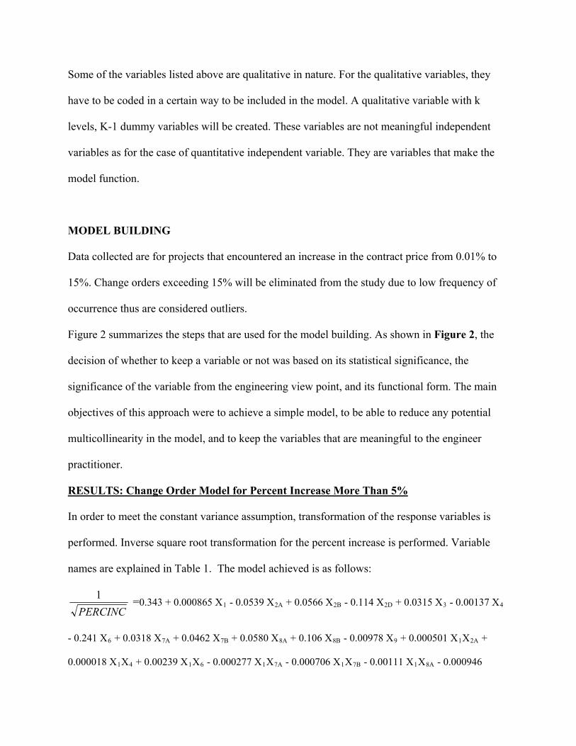
In order to meet the constant variance assumption, transformation of the response variables is

performed. Inverse square root transformation for the percent increase is performed. Variable

names are explained in Table 1. The model achieved is as follows:

PERCINC

1 =0.343 + 0.000865 X1 - 0.0539 X2A + 0.0566 X2B - 0.114 X2D + 0.0315 X3 - 0.00137 X4

- 0.241 X6 + 0.0318 X7A + 0.0462 X7B + 0.0580 X8A + 0.106 X8B - 0.00978 X9 + 0.000501 X1X2A

0.000018 X

+

1X4 + 0.00239 X1X6 - 0.000277 X1X7A - 0.000706 X1X7B - 0.00111 X1X8A - 0.000946

X1X8B -0.0513 X2BX7A - 0.0567 X2BX8B + 0.0133 X2BX9- 0.102 X2DX3 + 0.0834 X2DX7 + 0.0961

X2DX7B + 0.0629 X2D X8A + 0.0578

X3X8B...........................................................................................Eq. 5

t factors

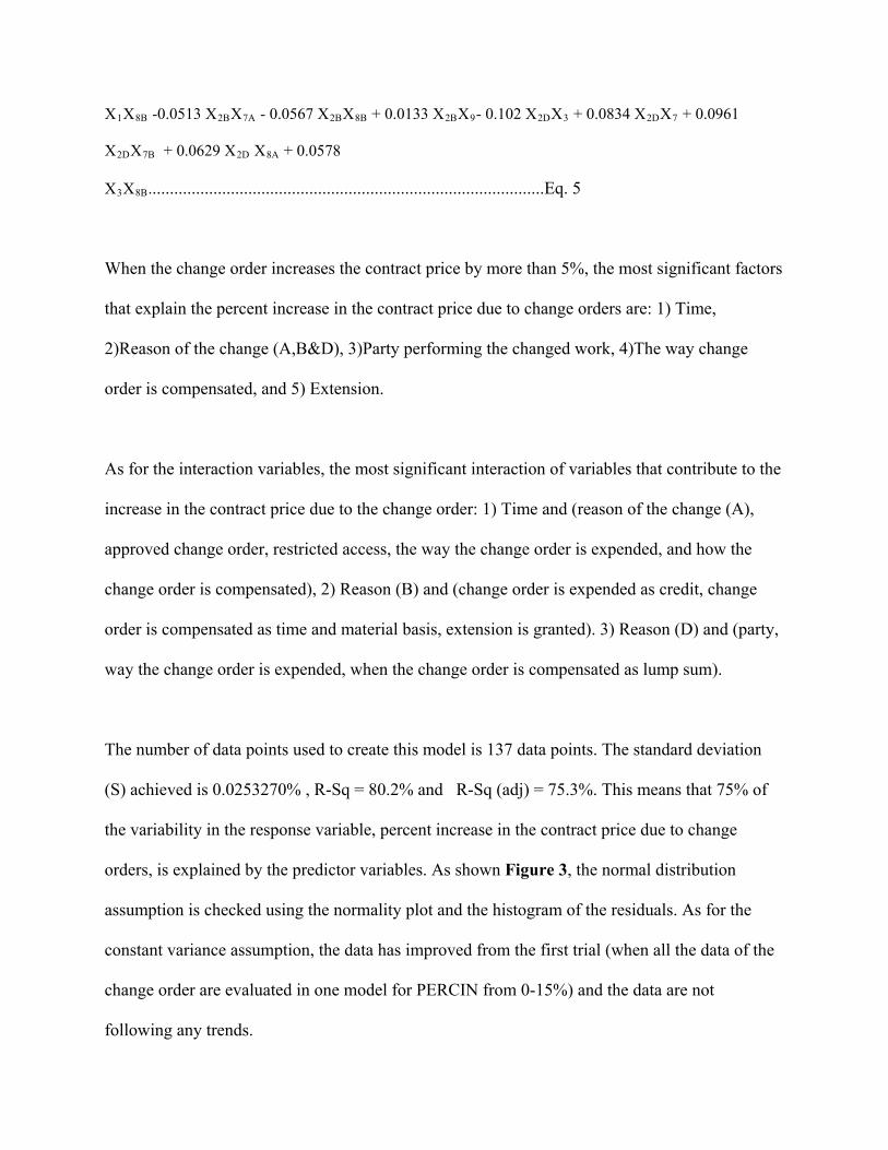
performing the changed work, 4)The way change

rder is compensated, and 5) Extension.

he

arty,

ay the change order is expended, when the change order is compensated as lump sum).

of

a of the

ated in one model for PERCIN from 0-15%) and the data are not

following any trends.

When the change order increases the contract price by more than 5%, the most significan

that explain the percent increase in the contract price due to change orders are: 1) Time,

2)Reason of the change (A,B&D), 3)Party

o

As for the interaction variables, the most significant interaction of variables that contribute to t

increase in the contract price due to the change order: 1) Time and (reason of the change (A),

approved change order, restricted access, the way the change order is expended, and how the

change order is compensated), 2) Reason (B) and (change order is expended as credit, change

order is compensated as time and material basis, extension is granted). 3) Reason (D) and (p

w

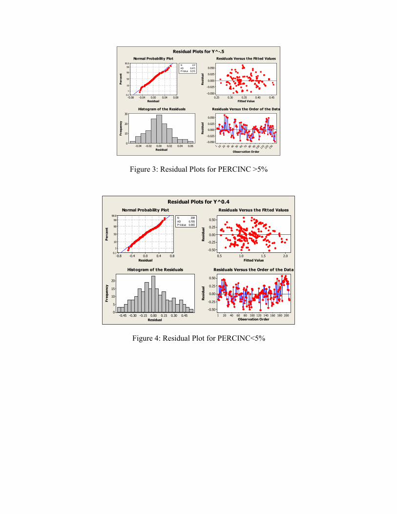
The number of data points used to create this model is 137 data points. The standard deviation

(S) achieved is 0.0253270% , R-Sq = 80.2% and R-Sq (adj) = 75.3%. This means that 75%

the variability in the response variable, percent increase in the contract price due to change

orders, is explained by the predictor variables. As shown Figure 3, the normal distribution

assumption is checked using the normality plot and the histogram of the residuals. As for the

constant variance assumption, the data has improved from the first trial (when all the dat

change order are evalu

RESULTS: Change Order Model for Percent Increase Less than 5%

In order to meet the constant variance assumption, transformation of the response variables is

performed for the percent increase. Variable names are explained in Table 1. The model

achieved is as follows:

PERCINC4.0 = 1.56 + 0.00763 X1 + 0.365 X2A + 0.139 X2B - 0.160 X2C + 0.295 X2D + 0.149 X3 + 0.00308 X4

+ 0.354 X5 - 0.947 X7A - 0.912 X7B + 0.256 X8A - 0.519 X8B + 0.00832 X9 - 0.00699 X1X2A - 0.00535 X1X

0.00535 X

2C -

7BX8B…………Eq. 6

d

order is

xperience change orders up to 5% and

ore than 5% is where problems of quantification arise.

nge (A&D), 3) Way the

e

hange

1X2D + 0.112 X2AX4 - 0.480 X2AX5 - 0.385 X2BX3 - 0.342 X2BX5 + 0.224 X2BX8B + 0.679X2CX8A +

0.850 X2CX8B - 0.263 X3X5+ 0.175 X3X7A - 0.401 X3X8B - 0.164 X5X7B + 0.594 X7AX8B + 0.759

X

The number of data points used to create this model is 208 data points. The model has a standar

deviation (S ) of 0.25959, R-Sq = 62.9% and R-Sq(adj) = 57%. This means that only 57% of

the variation of the response variable percent increase in the contract price due to change

explained by the predictors. This is a considerably low value of R-Sq (adj), however as

supported by the literature most of construction projects e

m

Most of the variables have a variable of inflation less than 100; a threshold which above

multicollinearity is present. The most significant factors that explain the percent increase in the

contract price due to change orders are: 1) Time, 2) Reason for the cha

change order is expended, 4) How the change order is compensated.

As for the interaction variables, the most significant interaction of variables that contribute to th

increase in the contract price due to the change order are: 1) Time and the reason of the c

(A&D), 2) Reason (A) and (approved change order hours), 3) Reason (B) and (the party

performing the change, and when the change order is compensated as time and material basis

Reason (C) and the way the change order is compensated, 5) Party and the when the change

order is compensated as time and material basis, and 6) The way the change order is expended

and when the change order is compensated as time and material basis. As shown in

), 4)

re 4,

he fitted value the variance is not following a trend, thus the

ssumption of constant error is met.

in the

most of the quantification

amage problems occur when change orders are higher than 5%.

d the

Figu

the normal probability plot and the histogram of the residuals the data follows a normal

distribution, and the residual versus t

a

MODEL VALIDATION

The validation data set consists of 29 observations from four projects that were not used

model building. The actual percent increase in the contract price due to change order is

compared to the predicted percent increase from the model. The average percentage of error is

28.61% for the change order model that quantify the percent increase in the contract price due to

change orders that exceed 5%, and 43.94% for the change order model that quantify the percent

increase in the contract price due to change orders less than 5%. The error value is slightly high

for the prediction model for change orders less that 5%, yet usually

d

CONCLUSION

The study tackled the change orders from verifiable site data. The researchers conducted several

interviews with a public owner and claims consultants who work for parties, the owner an

contractor. The change order model provided a tool to the owner to perform a forward or

retrospective pricing of change orders. It aids in forecasting the cash flow of the owner and to

make sure that the contingency money available for the project will cover the cost of the c

orders. In addition, the research provided a tool to help the owners in heavy construction

projects, a trade that was seldom studied, to quantify the cost of the change orders at different

period of times during the lifetime of the project. In the presence of the change order model,

where both parties agree upon, the process of handling the changes and the quantification of the

damage will be easier and hence the owner

hange

’s and the contractor’s time and money allocated for

e dispute resolution will be minimized.

re

his

h

y the industry and is lacked in the curriculum; either for a graduate or undergraduate

rograms.

th

RELATION TO THE CURRICULUM DEVELOPMENT:

Change orders and their effect on productivity is an important aspect to our industry and a

seldom mentioned in current Construction Engineering and Management programs. T

research was the base for the development of two graduate courses. The first one is”

Construction Labor Productivity Management”. This course focuses on external factors that

affect labor productivity on the site and in particular the effect of change orders. The present

research opened the door of how to analyze their change orders and quantify their impact on

productivity loss. The second course developed from this research is another graduate course

called “Construction Claims”. In any claim, the most important point is to be able to provide a

cause effect analysis to support the entitlement for the claimed amount. The present researc

showed a methodology to be able to win the claim; a big section that will be taught in this

course. In a nutshell, this research provided a baseline for highlighting important concepts that

are needed b

p

REFERENCES

1. Finke, Michael “A Better Way to Estimate and Mitigate Disruption” Journal of Construction Engineering

m” Calculating Lost labor Productivity in Construction Claims” John Wiley &Sons

3. Chick, David “The Time Value of Project Change” Journal of Cost Engineering, Vol.41/No.6, June 1999.

LIST OF FIGURES

and Management, November 1998, 490-497.

2. Shwartzkoph, Willia

Inc., Canada, 1995.

Explain Research Objective

Contact District Construction Office &

Hold Meeting

Collect Data from Each District

Start Data Preparation for Model Building

Study the Projects Selected:

Problem areas, reason for changes/claims

Identify Projects Criteria • Road Projects/Design-

Bid-Build/100%

completed/Claims are

resolved

Identify Documents Required for each

Project Selected • Contract

• Daily Reports

• Change Orders Issued

Figure 1: Data Collection Procedures

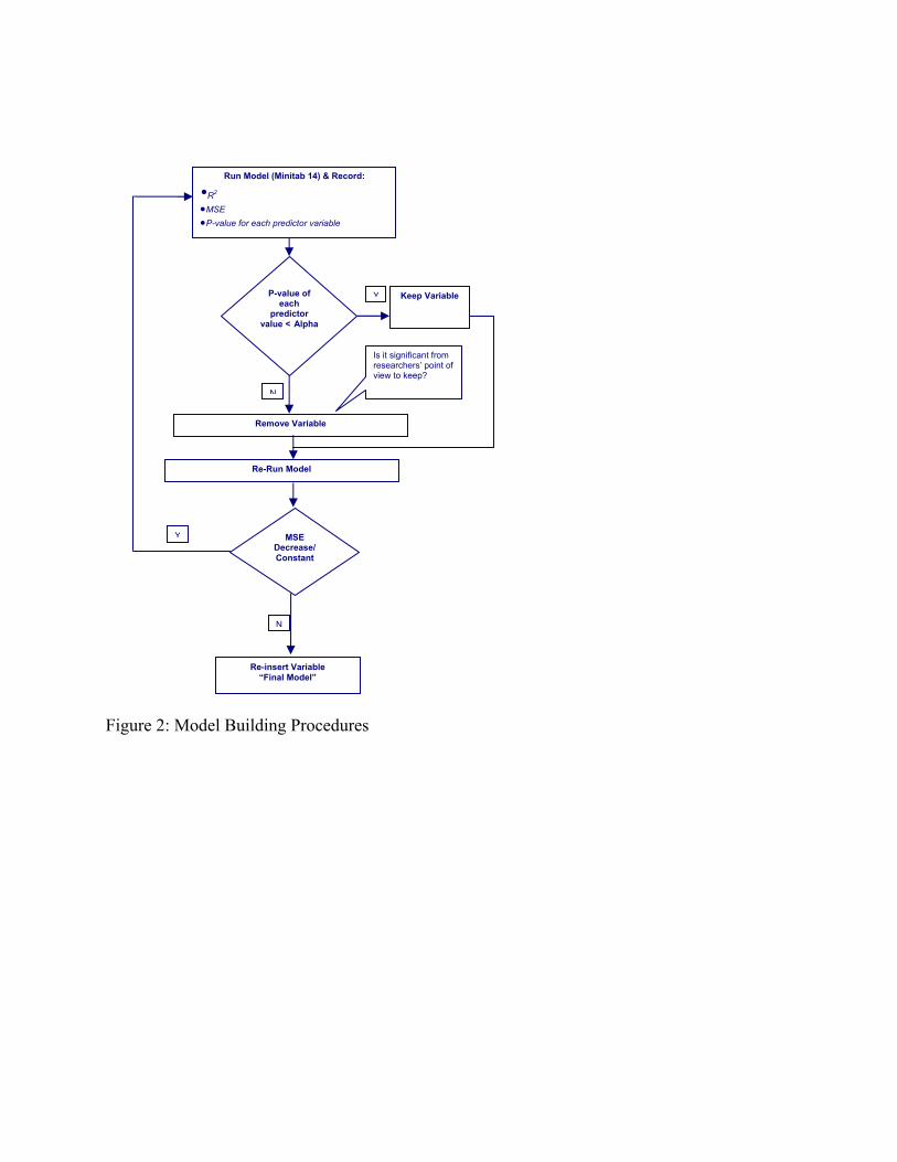
Figure 2: Model Building Procedures

Re-insert Variable

“Final Model”

N

Remove Variable

Is it significant from researchers’ point of view to keep?

Keep Variable YP-value of each

predictor

value < Alpha

Y

Run Model (Minitab 14) & Record:

•R2

‚MSE

‚P-value for each predictor variable

Re-Run Model

MSE Decrease/

Constant

N

Residual

Pe

rce

nt

0.080.040.00-0.04-0.08

99.9

99

90

50

10

1

0.1

N 137

AD 0.471

P-Value 0.241

Fitted Value

Re

sid

ua

l

0.450.400.350.300.25

0.050

0.025

0.000

-0.025

-0.050

Residual

Fre

qu

en

cy

0.060.040.020.00-0.02-0.04

30

20

10

0

Observation Order

Re

sid

ua

l

130

120

110

1009080706050403020101

0.050

0.025

0.000

-0.025

-0.050

Normal Probability Plot Residuals Versus the Fitted Values

Histogram of the Residuals Residuals Versus the Order of the Data

Residual Plots for Y^-.5

Figure 3: Residual Plots for PERCINC >5%

Residual

Pe

rce

nt

0.80.40.0-0.4-0.8

99.9

99

90

50

10

1

0.1

N 208

AD 0.705

P-Value 0.065

Fitted Value

Re

sid

ua

l

2.01.51.00.5

0.50

0.25

0.00

-0.25

-0.50

Residual

Fre

qu

en

cy

0.450.300.150.00-0.15-0.30-0.45

20

15

10

5

0

Observation Order

Re

sid

ua

l

200180160140120100806040201

0.50

0.25

0.00

-0.25

-0.50

Normal Probability Plot Residuals Versus the Fitted Values

Histogram of the Residuals Residuals Versus the Order of the Data

Residual Plots for Y^0.4

Figure 4: Residual Plot for PERCINC<5%

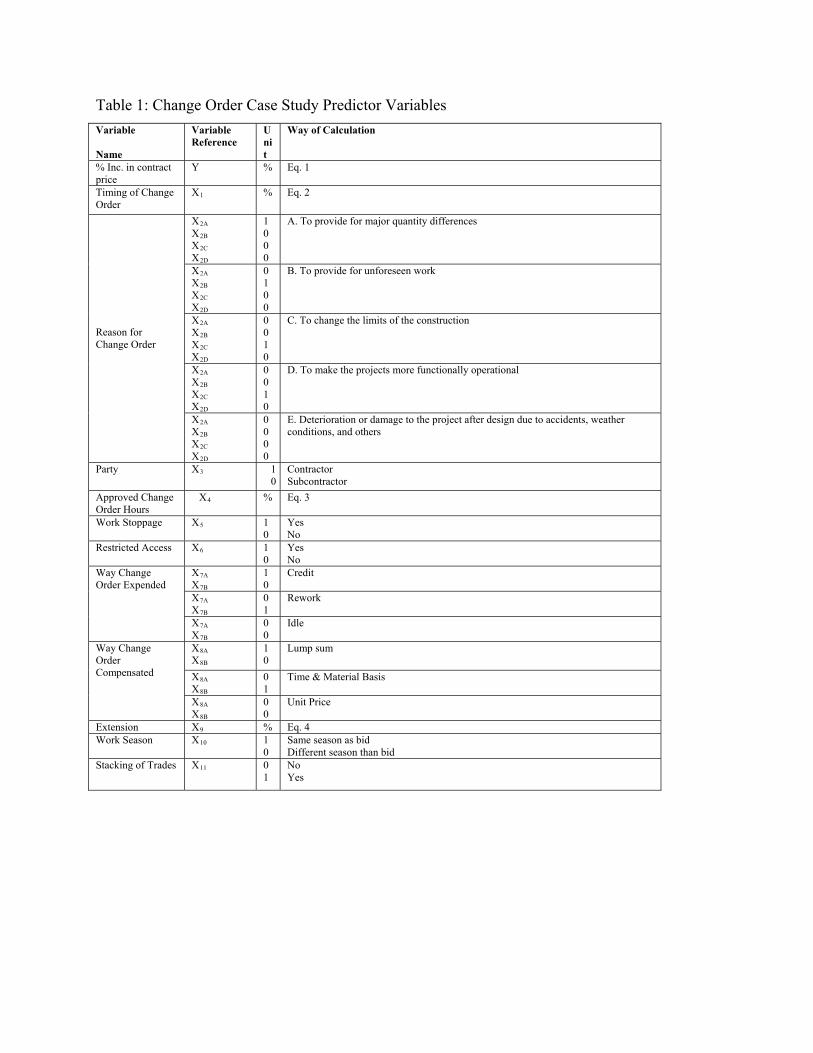
Table 1: Change Order Case Study Predictor Variables

Variable

Name

Variable

Reference

U

ni

t

Way of Calculation

% Inc. in contract price

Y % Eq. 1

Timing of Change Order

X1 % Eq. 2

X2A X2B X2C X2D

1 0 0 0

A. To provide for major quantity differences

X2A X2B X2C X2D

0 1 0 0

B. To provide for unforeseen work

X2A X2B X2C X2D

0 0 1 0

C. To change the limits of the construction

X2A X2B X2C X2D

0 0 1 0

D. To make the projects more functionally operational

Reason for Change Order

X2A X2B X2C X2D

0 0 0 0

E. Deterioration or damage to the project after design due to accidents, weather conditions, and others

Party X3 1 0

Contractor Subcontractor

Approved Change Order Hours

X4 % Eq. 3

Work Stoppage X5 1 0

Yes No

Restricted Access X6 1 0

Yes No

X7A X7B

1 0

Credit

X7A X7B

0 1

Rework

Way Change Order Expended

X7A X7B

0 0

Idle

X8A X8B

1 0

Lump sum

X8A X8B

0 1

Time & Material Basis

Way Change Order Compensated

X8A X8B

0 0

Unit Price

Extension X9 % Eq. 4

Work Season X10 1 0

Same season as bid Different season than bid

Stacking of Trades X11 0 1

No Yes