NBER WORKING PAPER SERIES

THE DETERMINANTS OF PUNISHMENT:DETERRENCE, INCAPACITATION AND VENGEANCE

Edward L. GlaeserBruce Sacerdote

Working Paper 7676http://www.nber.org/papers/w7676

NATIONAL BUREAU OF ECONOMIC RESEARCH1050 Massachusetts Avenue

Cambridge, MA 02138April 2000

Both authors thank the National Science Foundation. Steven Shavell, Steven Levitt, and participants in theNBER Law and Economics group provided helpful comments. The views expressed herein are those of theauthors and are not necessarily those of the National Bureau of Economic Research.

2000 by Edward L. Glaeser and Bruce Sacerdote.. All rights reserved. Short sections of text, not toexceed two paragraphs, may be quoted without explicit permission provided that full credit, includingnotice, is given to the source.

The Determinants of Punishment: Deterrence, Incapacitation and VengeanceEdward L. Glaeser and Bruce SacerdoteNBER Working Paper No. 7676April 2000

ABSTRACT

Does the economic model of optimal punishment explain the variation in the sentencing of

murderers? As the model predicts, we find that murderers with a high expected probability of

recidivism receive longer sentences. Sentences are longest in murder types where apprehension rates

are low, and where deterrence elasticities appear to be high. However, sentences respond to victim

characteristics in a way that is hard to reconcile with optimal punishment. In particular, victim

characteristics are important determinants of sentencing among vehicular homicides, where victims

are basically random and where the optimal punishment model predicts that victim characteristics

should be ignored. Among vehicular homicides, drivers who kill women get 56 percent longer

sentences. Drivers who kill blacks get 53 percent shorter sentences.

Edward L. Glaeser Bruce SacerdoteDepartment of Economics Department of Economics327 Littauer Center 6106 Rockefeller HallHarvard University Dartmouth CollegeCambridge, MA 02138 Hanover, NH 03755and NBER and NBEReglaeser@kuznets.harvard.edu bruce.i. sacerdote@dartmouth.edu

I. Introduction

The economic approach to punishment pioneered by Bentham (1823) and Becker (1968) is

normative. Their work, and the literature that has followed, analyzes "how many resources and

how much punishment should be used to enforce different kinds of legislation?" (Becker, 1968).

But is this normative theory of optimal deterrence also a good positive theory of punishment?

Are prison sentences meted out in a way that corresponds with the implications of Becker's

model? Can we explain the differences in sentence lengths with a theory where punishment is

meant only to incapacitate and deter, or do we need a theory that also incorporates a taste for

vengeance?1

This paper examines the detenninants of punishment by examining the sentences given out to

murderers in the U.S. Using Bureau of Justice Statistics data on murders, we test the basic

implications of the economic model. Becker (1968) argues that sentences should be longer when

apprehension rates are lower. Indeed, across murder types, we find that sentences are highest

when the expected apprehension rate for murderers is lowest.

An optimal deterrence model also suggests that punishments should be stiffer in crimes where

the deterrence elasticities are greater. We do not have direct measures of deterrence elasticities

across types of homicide, but it is likely that inelastically supplied crimes will have less variance

across cities (see Appendix 1). For inelastically supplied crimes, cross-city differences in

probabilities of arrest or returns to crimes will cause less variation. As such, we use cross-city

crime variances as a proxy for deterrence elasticities and we find that sentences are stiffer from

murder types that appear to be less elastic.

A third implication of optimal punishment is that criminals with higher recidivism rates should

be incarcerated for longer periods. Using data from the Bureau of Justice Statistics "Recidivism

of Felons on Probation 1986-1989," we predict the probability of recidivism for each murderer.

This probability is based on the murderer's past record, demographic characteristics and type of

crime. We then correlate predicted recidivism with sentence length and find that murderers with

Bentham asserts that the only function of puthshment is to reduce crime through deterrence and incapacitation. Heviews the taste for vengeance as illegitimate. Becker does not incorporate a taste for vengeance into the model, buthe does not argue against catering to that taste.

2

higher recidivism rates receive stiffer penalties. Thus, in these three tests, the optimal

punishment model appears to actually predict the variation in sentence lengths

However, in a fourth test of the optimal punishment model, it becomes clear that there is more to

sentencing murderers than optimal deterrence and incapacitation. The optimal punishment

model suggests that victim characteristics will not matter when the victim is determined at

random. Using two data sets on vehicular homicides, we look for the importance of victim

characteristics. In the Bureau of Justice Statistics national data set, we find that victim race, age

and criminal record still determine sentence length even when the victim was killed in a

vehicular homicide. Drivers who kill black victims get substantially shorter sentences. Drivers

who kill women get substantially longer sentences. Indeed, there is no difference in the

magnitude of victim effects (when using the logarithm of sentence length) between vehicular

homicides and other types of murder. In a data set on vehicular homicides in Alabama, we still

find that there is a substantial victim gender effect. There is no statistically discernable victim

race effect in these data.

One proposed explanation for the above findings is that sentence lengths are driven, in part, by a

taste for vengeance. Since this taste may operate at a subconscious level, it would not be

surprising if victim characteristics still motivate this taste, even when the victim is random. The

presence of victim effects in vehicular homicides suggests to us that the taste for vengeance is an

important determinant of actual sentence lengths. However, one should not ignore the fact that

the basic optimal punishment model has a great deal of explanatory power. Both optimal

punishment and a taste for vengeance appear to drive sentencing in homicides.

II. The Determinants of Punishment

In this section, we summarize the predictions of a version of the basic Becker framework. The

general formula for optimal punishment begins with the behavior of murderers. We assume

there is a supply of murders, denoted Me), which is a function of the probability of

apprehension, denoted P, times the severity of punishment, denoted S. To satisfy second order

3

conditions, we assume that this function is declining and convex. We will treat the probability of

apprehension as exogenous and solve for the optimal severity of punishment.2

The social loss from the death of a victim is denoted V. This loss is meant to include the loss to

the victim and to the rest of society. The social cost of imposing a sentence of severity S on a

criminal of type T is C times S. This cost is meant to be high for individuals who produce much

for society at large. The social cost of prison will be low for people with high recidivism rates

who are likely to commit socially damaging crimes if they are released. The social planner then

would choose the level of severity to minimize M(PS)[V+PCS}. Optimization produces the

M eTM M PSM'(PS)formula S = *, where s = — , the elasticity of the murder rate with

Pc (i—c) M(PS)

respect to the quantity of punishment.

If this elasticity is treated as a constant parameter, then this equation yields four comparative

statics that are at the core of the normative implications of economic approach to punishment.

Severity (i.e. sentence length) should be higher when the deterrence elasticity is higher. Severity

should be higher when the victim is valued more by society, or when the recidivism rate is high.

Increases in deterrence elasticity should increase sentence length. As the probability of

apprehension rises, the sentence length should fall. We will test all of these hypotheses.

One thing that the optimal deterrence model does not predict is that random features of the crime

should be part of the punishment. Punishing criminals on the basis of the random characteristics

of criminals just introduces extra randomness into sentencing and serves no purpose according to

this model.3 Randomness in punishment is undesirable for many reasons. For example, it may

be that costs of punishment to the victim rise more slowly with randonmess than the costs of

punishment to the state (see Polinksy and Shavell, 1984, for a discussion).4

Ill. Data Description

2 Our basic set-up builds upon that of several authors including Becker (1968), Posner (1981), Polinsky and Shaveil,(1984).

If the conditions that make random punishment undesirable are not met, then this just means that we should seerandom punishment, not punishment based on the random characteristics of victims.

Note that many features of the criminal justice system, such as sentencing guidelines, are designed to reducerandomness in punishment. See for example published reports from the Massachusetts Commission for SentencingGuidelines.

4

Our first data set is the Bureau of Justice Statistics "Murder Cases in 33 Large Urban Counties."

This is a random sample of homicide cases drawn from prosecutors' files. The data set includes

information on offender characteristics, victim characteristics and trial outcomes for 2800

murders. The 75 largest counties account for more than half of the murders in the U.S each

year. This data set brings together information on the crime, the offender, the victim., and the

sentence. Such information cannot all be linked in other larger data sets such as the Uniform

Crime Reporting (UCR) Data or the National Crime Victimization Survey (NCVS). Most crime

data sets are institutionally based, so that the Department of Corrections can tell us about the

number of prisoners moving in and out of the prison system, or the FBI can give us numbers on

complaints and arrests. But such data sets do not allow us to follow an offender and victim from

the commission of the crime, through arrest, the judicial system and sentencing.

When we compare the circumstances of the murders in our data set with the data in the much

larger Uniform Crime Reports Supplementary Homicide Reports, the distribution across

homicide types (circumstances) is similar. Appendix Table 1 gives a complete set of means and

standard deviations for our primary data set. While we have solid data on the prior criminal

history of both the criminal and the victim, we have only limited other demographic information

on each individual. We know age, gender and race and for a subsample of the data we have hand

coded occupational information. We use the mean income in the occupation as a proxy for tme

income.5

All of these cases are ones in which a homicide related charge was filed. In our data, 76 percent

of the cases led to a conviction. Table 2 presents an overview of conviction rates by types of

homicides. Of these cases, less than 1 percent of offenders receive the death penalty and 9

percent receive life in prison. As we will generally attempt to work with a single attribute

"sentence length," there is an issue as to how we treat life sentences. We will generally treat a

life sentence as a 50 year sentence, but our results are robust to alternate treatments of life

sentences.

Table I also presents an overview of sentence lengths and conviction rates by types of murder.

The harshest penalties appear to be levied against arsonists (50 years), although there are only 5

convicted arsonists in the sample, so this is surely measured with considerable error. Given the

S

possibility that arson can create truly horrendous social costs, it seems reasonable that this crime

is particularly singled out for a severe penalty. Among the other crime categories, murders that

are done by professional criminals in the course of other crimes receive harsh penalties (close to

30 years in many cases). Murders that are the result of arguments that are not part of other

crimes, appear to receive much shorter sentences, around 15 years. In general, murderers serve

approximately 50 percent of the length of the sentence to which they are convicted.6

One testable explanation for these findings is that they provide support for the marginal

deterrence hypothesis (Stigler, 1970). According to this hypothesis, because criminals are

already receiving severe penalties for their first crimes, to deter murder, tougher sentences must

occur for combining the crimes. To check for this possibility, we examine the correlation

between sentence length in crimes without murder and sentence lengths, for the same crimes,

when there is a murder.7 Across crime categories there is no relationship between the non-

murder sentence (which should be interpreted as the sentence for the crime if murder had not

occurred) and the murder sentence (which should be interpreted as the cumulative sentence for

both the murder and the other crime). This casts some doubt on whether America is generally

following a policy of marginal deterrence.

The Alabama Data: To construct a second micro-data set on vehicular homicide cases, we

obtained data from the Alabama Administrative Office of Courts and a number of Alabama State

offices. We merged data on offenders from court records with data on victims from the FBI

Supplementary Homicide Reports, death records from the Alabama Office of Health Statistics,

and accident records of the Alabama Department of Public Safety. For each victim, we know

age, sex, and race. The conviction rates and sentence lengths are comparable to those found in

our main BJS data set.

IV. Optimal Punishment

In this section, we describe the construction of variables relating to the role of deterrence,

incapacitation and sympathy for either the victim or the perpetrator. We then test for the

importance of these variables.

A non-trivial number of occupations were in the illegal sector (e.g. prostitute, mafia bodyguard). In those cases,we ised the closest legal occupation.6 See the Sow-cebook of Criminal Justice Statistics or various BJS Publications.

6

Deterrence Elasticities: To test the importance of deterrence, we want to see whether types of

murder that have higher deterrence elasticities receive stiffer penalties. Ideally, one would use

exogenous sources of variation in the level of punishment over space and test whether different

types of crime respond differentially to these different punishment levels. However, the studies

that use exogenous variation in arrest rates (e.g. Levitt, 1998) do not distinguish between types of

homicides.

An alternative approach, which is sketched in Appendix 1, is to rely on the variation of murder

rates for different types of murder over space. As the appendix illustrates, differences in the

coefficient of variation across different types of crime are a function of the deterrence elasticity

of the crime rate and other differences over space in the attractiveness of particular types of

crime. The intuition of this effect is that if regions differ in their level of deterrence, then the

murder types with high deterrence elasticities will have big variation in their levels of space.

The murder types with low deterrence elasticities will have less variation over space.

Unquestionably, this is a noisy measure of the deterrence elasticity, but it is the best available to

us.

Figure 1 shows the relationship between this measure of deterrence elasticity and sentence

lengths across types of crimes. In general there is a positive relationship and the relationship is

significant. Murders resulting from lover's quarrels and other arguments have the least variation

(and probably the lowest deterrence elasticities) and the lowest punishment.

Probability of Apprehension: The next prediction of the Becker framework is that crimes where

probabilities of apprehension are low will be punished more severely. The Supplementary

Homicide Reports can be used to determine whether or not the police consider the case cleared

by arrest. While this is not exactly the apprehension rate, it is a good proxy.

Figure 2 shows the relationship between this apprehension rate variable and the average sentence

length. The relationship is negative, as predicted. The correlation across homicide types

between sentence and apprehension rates is —38 percent. Lover's quarrels, arguments and brawls

under alcohol have the highest probabilities of apprehension and the lowest sentence lengths.

Available upon request. In the interest of space, we did not include these results.7

Arson has a particularly low probability of apprehension and the highest average sentence length.

Of course, long prison sentences for arsonists may have more to do with the great potential for

social damage created by arson.

Incapacitation: We are particularly interested in measuring the propensity of various murderers

to commit further crimes. As high recidivism rates will lead to high elasticities of crime quantity

with respect to sentence lengths and as high recidivism rates reduce the average social cost of

putting someone in prison, individuals with a high propensity for recidivism will be more likely

to receive stiffer sentences. Our approach is to create a predicted recidivism measure for each

offender and to include that as a variable that might explain sentence length.

We use data from the Bureau of Justice Statistics "Recidivism of Felons on Probation 1986-

1989" data set. In Appendix Table 2, we show the result of a probit where the dependent

variable is "committing a violent crime while on parole." In this regression, we find that crime

characteristics tend to be quite important. Individuals who are guilty of robbery are very likely

recidivists. Gender, race and number of priors also matter. Our recidivism measure is

essentially an index that is higher for men, blacks, criminals with more prior arrests and

individuals who are guilty of robbery and assault.

One problem with this data set is that we have a data set on recidivism for all criminals and we

are considering the punishment of murderers only. (There are no sizeable data sets on the

recidivism of murderers.) Certainly, this is problematic but we have no reason to believe that the

same characteristics that predict recidivism among standard felons do not predict recidivism

among murderers as well.

In Figure 3, we show the relationship between recidivism and sentence length. Recidivism also

predicts sentence length. Lover's quarrel murders are again at the low end of the recidivism

scale and the low end of sentence length. Robberies are at the high end of the recidivism scale.

The fact that arguments and lovers' quarrels have low sentence lengths and are low on

deterrence, and recidivism and high on apprehension suggests that several theories exist to

explain sentence lengths for many crimes.

Table 2: In Table 2, we explore these variables in a simple regression setting. In this case, the

unit of observation is the murder. In the cases of the elasticity measure and the apprehension8

rate, there is only variation across type of homicide. The recidivism measure differs also by

offender characteristics. In all cases, the standard errors have been corrected to address the fact

that we do not have meaningifil heterogeneity across all of the observations in the regression.

In the first regression, we examine all three variables without any other controls. All three

variables are both quantitatively and statistically significant. A one-standard deviation increase

in the recidivism measure increases the sentence length by 12 percent (which is .1 standard

deviations). Sentence length rises with the elasticity measure and falls sharply with the

apprehension rate. As the apprehension rate increases by 10 percent, the sentence length falls by

almost the same amount. This quite remarkable result is the exact prediction of some versions of

the optimal deterrence model where expected punishment should be kept constant across types of

crimes. If anything we would expect the endogeneity of apprehension rates to mean that this

parameter is underestimated, because more effort may be put into apprehending more dangerous

murderers who are then given stiffer sentencing.

The second regression includes controls for conviction type. Much of the variation in sentencing

depends on whether the murderer is convicted of first degree murder, second degree murder or

manslaughter. The jury ultimately decides the conviction type. The judge, who is subject in

many cases to sentencing guidelines, determines the sentence after conviction.8 We find that

controlling for conviction type makes no difference to the recidivism variable. Apparently, the

coimection between recidivism and sentence length works through sentencing, post conviction,

not through the actions ofjuries. Most of the effect of the elasticity measure disappears when we

control for conviction type. Forty percent of the apprehension rate effect disappears when we

include conviction type dummies.

The third regression includes controls for victim and offender characteristics. Our results on the

recidivism, variation and apprehension rates are not altered by these controls. There are very

striking effects of victim characteristics. Murderers who kill black victims receive 26.8 percent

shorter sentences.9 Murderers who kill male victims receive 40,6 percent shorter sentences. It

also appears to be true that when the victim is older the sentence is longer. The income variable

is positive—richer victims appear to lead to longer sentences—but it is not significant.

All of our results are robust to including state and county fixed effects

9

One interpretation of our race, gender and age effects is that society values women, whites and

the elderly more and therefore optimal punishment calls for stiffer sentences of murderers who

kill these victims. However, there is little evidence that suggeststhat our society values women

more than men. Lichtenberg (1998) shows we generally spend slightly less researching diseases

the afflict women. In civil cases where there are value of life judgements, male lives are

generally attributed a higher value. Many people believe that society discriminates against

women, not for them. The racial effects on sentencing may be despicable, but are still readily

explained under racist preferences and optimal punishment given those preferences The gender

effect is more of a puzzle, which we will return to at the end ofthe paper.

Table 3 shows the results of regressing sentence length on characteristics of the victim and

perpetrator. In the first regression we regress the log (sentence years) for convicted murderers as

a function of victim characteristics, murderer characteristics and circumstance dummies.'° In

general, characteristics of both the victim and the offender tend to be quite important. A male

offender receives on average a .47 log point increase in his sentence relative to a female

offender. Offender age is insignificant. African-American offenders appear to receive slightly

longer sentences but this effect is not statistically significant. Hispanic offenders do not receive

longer sentences.

Offenders with more violent prior convictions receive much stiffer sentences. Controlling for

this variable is the crucial step towards eliminating the impact of offender race on sentence. One

interpretation of this fact is that there is no offender race effect on sentencing. Alternatively, past

discrimination may have lead to more violent prior convictions prior to this current crime, so

controlling for this variable could cause an erroneous conclusion of no racial prejudice towards

black offenders.

The victim characteristics are also quite significant. Offenders who kill male victims receive

much shorter sentences. One interpretation is that male victims are more likely to have initiated

the conflict. We have been able to partially reject this interpretationby examining only murders

where the offender was the aggressor, and in those cases the victim's gender is still quite

important.

Throughout the paper. we adopt the convention of referring to log pointdifferences as percent differences.

10

The race of the victim is also quite important. Perpetrators who kill blacks and hispanics are

much less likely to receive stiff sentences than perpetrators who kill whites. There is no real

cross effect between the race of the offender and the race of the perpetrator. When victims are

gang members, sentences appear to be shorter by a sizable margin, but this effect is not

statistically significant. Note from Appendix Table 1 that only 5% of the victims are gang

members. It is also true that when there are more victims, the sentences are stiffer. Killing a

victim with a past criminal record yields a shorter sentence.

Victims over the age of 65 are associated with much stiffer sentences. Young victims (less than

12 years old) are associated with lower sentences. This latter effect reflects the fact that younger

victims are ofien in child abuse cases for which sentences are lower on average. When the

victims are unemployed or prostitutes, sentences are shorter. We find that the female gender

effect is significantly reduced when the victim is a prostitute. One interpretation of this finding

is that society values these people less. An alternative view is that the taste for vengeance is

closely tied to the innocence of the victim.

The impact of offender race and gender is not new. For example, Baldus eta!. (1988) show that

death sentences are much rarer when the victim is black. Gross and Mauro (1998) show that

death sentences are more common when African-Americans kill whites. Spolm (1994) shows

the impact of victim race in sexual assault cases. While in a sense, we are only confirming a

well known race of victim effect, given the general nature of our data set, we think that finding

this effect in a national homicide sample is particularly important.

We also include a wide range of crime circumstance dummies. These are always significant and

they always take the predicted signs. For example, it is always true that when the victim

"provoked" the attack, the sentences are much shorter. Sentences are longer when the murder

took place in the context of a professional crime. Vehicular homicide offenders get by far the

shortest sentences.

In the second, third and fourth regressions, we examine the role that sentencing and conviction

play in determining the length of sentence. Regression (2) reports marginal effectsfrom a probit

regression where the dependent variable is whether the prosecutor brought a charge of first

° All regressions are robust to including county fixed effects.11

degree murder against the defendant. Murder one was actually charged in a majority of our

cases. There is a substantial race effect in which black victims are associated with fewer murder

one charges. Circumstance factors are also important. The gender of the victim is not correlated

with charging murder one. Other than past offenses, perpetrator characteristics are uncorrelated

with being charged with first degree murder.

In the third regression, we look at the probability of being convicted in a first degree murder

case. Here the gender effect appears strongly. Cases where women are victims are much more

likely to result in murder one convictions than other cases. Again, the race of the victim also

matters and when the victim is white, a murder one conviction is much more likely. The priors

of the victim are also very important. Since the victim effects really appear to matter at the

conviction stage, we suspect that it is a taste for vengeance among juries and prosecutors that

really matters.

The fourth regression looks at sentencing, controlling for conviction type. The gender effects are

weaker than without conviction type dummies but they are still quite significant. The coefficient

on victim male drops from -.4 15 to -.260, but remains quite significant. One way to interpret this

change is that forty percent of the gender effect is being determined by differential conviction

rate and sixty percent by post-conviction sentencing. Victim income and age also matters in this

stage. The dummies for type of conviction are naturally incredibly strong for predicting the

sentence length.

Tables 4a-4d present evidence on sentence rates as a ifinction of the race and gender of the

murderer and the victim.'1 These tables help us to think about whether there are interactions

between the race of the offender and the race of the victim. They also present our results in a

simple fashion. In Table 4a, we show the mean sentence length by the race of the murderer and

the victim. Without including any other controls, we find that white murderers receive a 3.7 year

shorter sentence if they kill a black person relative to a white person and black murderers receive

a 5 year shorter sentence if they kill a black person. Without including other controls, it also

appears that black offenders get longer sentences. If the victim is white, then black offenders

appear to get a 3.3 year stiffer sentence and if the victim is black then black offenders appear to

receive a 2 year longer sentence.

12

Table 4b shows that the gender effects are even more striking. Male offenders receive a 6.2 year

longer sentence than female offenders if the victim is female and a 6.9 year longer sentence if the

victim is male. Killing a woman also results in a substantially longer sentence. For male

offenders, killing a woman increases the sentence length by 4.2 years. For female offenders,

killing a woman results in a 4.9 year longer sentence. In the Alabama data set we find a

significant victim gender effect with female perpetrators, but not with male perpetrators.

One issue with these results is that gender and race may be correlated with attributes of the

murder that are not observable. To try and address this issue, and to further test the optimal

punishment hypothesis, we now turn to a narrow class of murders: vehicular homicides.

V. Vehicular Homicides

Vehicular homicides have the advantage that they are a relatively homogenous crime category.

Overwhelmingly, they involve substance abuse and reckless driving. To a first approximation, it

seems most likely that conditional upon the characteristics of the offender, the victimis random.

As such, optimal punishment clearly suggests that victim characteristics should not matter, or at

the very least should matter much less than in other homicides. Unfortunately, we have

relatively few vehicular homicides in the Bureau of Justice Statistics (142). We cast a wide net

going state-by-state to try and accumulate more records. Only in Alabama were we able to

accumulate more cases (another 46).

Tables 4c and 4d show the basic results on vehicular homicides. The gender effects remain and

seem to be about as strong as in the case of murders overall. In the Bureau of Justice Statistics

data, the gap for male offenders between male victims and female victims is 5.1 years. The gap

for overall homicides was 5 years. In the Alabama data, the gap is smaller: 2.77 years. The BJS

data also appear to show strong offender gender effects.

Table 5 shows our results in a regression setting. In the first regression we include all of our

vehicular homicides. Forty-eight of these observations involve victims who are pedestrians or

people in other ears. The remaining cases involve people in the offender's car. Since these are

These are raw means include all people charged. The raw differences (in terms of years) are similar when we

13

less likely to be random, in the second regression we include only cases where the victim is a

pedestrian or driving in another car. In both regressions, there are substantial victim gender

effects. Victim race remains quantitatively large in the second regression, but becomes

statistically insignificant. The past criminal history of the victim is quite important in both

regressions. It seems that drunken drivers who are "lucky" enough to run over males with a

criminal history face shorter sentences than drivers who run over innocent women. The third

regression gives results for the Alabama data set. Again, there is a substantial gender effect.

There is no race effect in the Alabama data set.

Overall, we believe that there are substantial victim effects that are strong even when the victim

is random. hideed, even if the victim is not purely random in the case of vehicular homicides,

there can be no doubt that there is substantially more randomness for vehicular homicides than

there is for other types of murders. At the very least, therefore, we would expect the effect of

victim characteristics to diminish for these types of homicide. However, the victim effects are

just as large as in cases where the murderer clearly selects the victim. These findings are

difficult to reconcile with the view that sentences reflect optimal punishment.

VI. Explaining the Results: The Taste for Vengeance

One alternative to the classical economic model of optimal punishment is that punishment

responds to tastes for vengeance among judges, juries and the citizemy as a whole. A rich set of

experimental results seems to confirm that human beings are often willing to sacrifice material

benefits to punish others; Romer (1995) develops an elegant model, which explains an

evolutionarily dominant taste for punishment. This taste for vengeance seems close to the

"outrage" model advanced in Sunstein (2000).

If punishment is based on the taste for vengeance of judges and juries, then the emotional

apparatus that determines the taste for vengeance may operate at a subconscious level and

therefore may not respond perfectly to unusual circumstances of the crime. For example, the

emotional response to victim characteristics will probably not be altered all that much even if we

know that the victim was essentially random. Because the taste for vengeance is not the outcome

of rational thought, the knowledge that the murderer did not select the victim may not alter the

condition upon conviction. The regressions that follow condition upon sentence >0.14

demand for vengeance. According to this view, there is likely to be a much stronger visceral

response to a drunk driver who accidentally kills an eight year old girl than to adrunk driver who

accidentally kills a 22 year old gang member. Thus, a taste for vengeance based view of

punishment may help us to understand our results on vehicular homicides.

Past social scientists have connected the taste for vengeance with the innocence of the victim.

Adam Smith (1759) in Theory of Moral Sentiments connected the taste for retribution to "our

sympathy with the unavoidable distress of the innocent sufferers." Smith emphasizes the extent

to which the victims are innocent as a determinant of the thirst for revenge.t2 If women are

thought to be mote innocent than men, then this may explain the pervasive gender effects. Our

results on victim criminal records and victims who are prostitutes are also easy to understand

using this idea. Anecdotally, we believe that the public is particularly anxious to punish men

who allegedly kill women (e.g. O.J. Simpson, Jack the Ripper, Klaus von Bulow, Sam Shepard),

or men who allegedly kill children (the Lindbergh baby kidnappers, Richard III).

Wile we have little evidence on these issues, as yet. Our suspicion is that the emotional

responses of juries are based upon (1) the degree to which they are able to identify with the

victim, and (2) the degree to which the victim is thought to morally pure. Kerr (1978)

documents the importance of victim innocence (as well as victim attractiveness) in mock jury

trials.

VI. Conclusion

We have presented evidence on the determinants of punishment for murderers in the United

States. We find the characteristics of the victim, the offender and the crime all generally matter.

Much of these effects can be understood as implications of an "optimal" punishment model

where punishments are higher when there is a greater value to incapacitation or a greater

deterrence elasticity. Some of our results can be understood as the outcome of a greater desire of

society to protect particular types of people.

2 Smith also emphasizes that "our heart rises up agahist the detestable sentnnents which influenced [vi11ains]conduct." This suggests the importance of intent and the state of mind of the perpetrator and might explain the rulesconcerning first degree murder.

15

However, we find the victim characteristics are also very important in vehicular homicides and

even in those vehicular homicides where the victim is a pedestrian. Optimal punishment theory

generally predicts that random aspects of the victim should not be important determinants of

punishment. But they are and this tends to supports a taste for vengeance view of the

determinants of punishment.

16

References

Baldus, D., Woodworth, 0. and C. Pulaski Equal Justice and the Death Penalty. Boston:Northeastern University Press, 1990.

Becker, 0. S. (1968) "Crime and Punishment: An Economic Approach," Journal of PoliticalEconomy.

Bentham, J. (1823) An Introduction to the Principles of Morals and Legislation. London: W.Pickering.

Gross, Samuel R. and R. Mauro, (1984) "Patterns of death: an analysis of racial disparities incapital sentencing and homicide victimization," Stanford Law Review 37, Nov. '84, 27-153.

Ken, Norbert L. (1978) "Beautiftil and Blameless: Effects of Victim Attractiveness andResponsibility on Mock Jurors' Verdicts," Personality and Psychology Bulletin 4(3): 479-482.

Levitt, S. (1997) " Using Electoral Cycles in Police Hiring to Estimate the Effect of Police onCrime," American Economic Review 87(3): 270-90.

Polinsky, M. and S. Shavell (1984) "The Optimal Use of Fines and Imprisonment," Journal ofPublic Economics 24:89-99

Posner, R. (1981), The Economics of Justice. Cambridge: Harvard University Press.

Romer, P. (1995) "Preferences, promises and the politics of entitlement," in Individual andSocial Responsibility (V. Fuchs, Ed.) Chicago: University of Chicago Press.

Smith, A. (1759) The Theory of Moral Sentiments. London: A. Millar.

Spohn, C. (1994) "Crime and the Social Control of Blacks: Offender/Victim Race and the

Sentencing of Violent Offenders," in Inequality, Crime and Social Control, ed. 0. S. Bridgesand M. A. Myers. Boulder, Co: Westview.

Stigler, 0. (1970) "The Optimum Enforcement of Laws," Journal of Political Economy 78(3):526-36.

Sunstein, C. (2000) Behavioral Law and Economics. Cambridge: Cambridge University Press.

Tonry, M. (1995) Malign Neglect--Race Crime and Punishment in America. New York: Oxford

University Press.

Walsh, A. "The Sexual Stratification Hypothesis and Sexual Assault in Light of the ChangingConception of Race," Criminology 25 (1987): 153-173.

Wolfgan, M. and M. Reidel "Race, Judicial Discretion and the Death Penalty," Annals of the

American Academy 407 (1973).

17

Appendix 1: Using the Variance of Crime Rates to Measure Relative Deterrence

We treat each subcategory of crime separately. In each location there is a distribution of private

net benefits of crimes. Within these net benefits we include the full range of psychic and

financial benefits from crime as well as the opportunity cost of time. The only component that is

specifically excluded is the costs of legal deterrence. We separate out these benefits into a

space-specific mean level of net benefits (denoted B) and a remainder "b." We assume that the

distribution of b is constant across space with cumulative distribution F(b) and density f(b).

There is also an expected level of deterrence, incorporating all of the expected punishment from

crime, which is denoted D, and which is assumed to differ over space but to be constant within

each location.

The quantity of criminals in each location are those for whom the benefits of crime B+b are

greater than the expected deterrence costs, D. There will be a marginal criminal, denoted b* for

whom b*=DB. The total quantity of crime in each location will equal lF(b*)=lF(D_B). The

elasticity of crime with respect to deterrence is _Df(b*)/(1_F(b*)).

We let D and B reflect the mean levels of D and B across the entire U.S. and let k=fl. Ifwe

take a Taylor series approximation for F) so that

(Al) Quantity of Crime per Capita = 1— F(b*) 1— F(b) — f(b)(D — B — D+ B).

Which means that elasticity of crime with respect to deterrence is Df(b*)/(1_F(b*)). Then

taking variances gives us that:

(A2) Variance of Crime Rates = f(b)2 Var(D — B),

or that:

(A3) LogI img = LogI + LoglD8Lflcrirne) L1—F()) P )

18

which means that the logarithm of the coefficient of variation of this crime equals the elasticity

(approximately) plus an error term relating primarily to the variance of the deterrence and net

benefits over space. If this variance is constant across crimes there will be no extra bias. If this

variance differs, then there will be a question that the elasticity is measured with error and

typically the coefficient on the elasticity will fall below the true elasticity value.

19

Table 1Prison Sentences By BJS Circumstance of Murder

Circumstances MeanSentence(years)

StandardDeviation

of Sentence

MeanConviction

Rate

NumberOf

Obs.

Robbery 32.3 17.9 .79 350

Burglary 32.1 17.5 .82 33

Sexual assault 36.3 17.9 .87 30

Arson 50.0 0.0 .83 6

Larceny 33.4 22.8 .71 7Auto theft 33.5 19.2 .92 25

Romantic triangle 14.7 12.5 .83 58

Property/money 17.1 16.5 .78 263

Redress of insult!personal honor 14.9 15.2 .77 256

Matters of opinion 18.2 17.3 .81 134

Lover/spouse quarrel 18.0 16.6 .81 305

Barroom dispute/brawl 13.2 14.7 .69 67

Street fight 12.5 15.2 .84 32

Punishment for stealing drugs/money 20.0 16.7 .84 25

Bad deal/bad drugs 15.8 12.5 .87 39

Money owed 22.6 17.2 .61 72

Stealing drugs/drug money 24.6 18.8 .71 73

Disputeoverdrugs 20.1 16.3 .80 113

Other gang fight between rival gang 10.7 7.2 .88 24

Contract killing/Hit for money 30.9 18.6 .70 53

Total 27.6 19.8 .76 3086Notes: These figures include life sentence and adjust it to be a 50 year sentence. Mean sentence is themean conditional upon conviction. Sample size includes convictions and non-convictions. Standarddeviations of conviction rates are p(l-p)".S and are not shown.

1

Table 2: The Determinants of Sentence Length

(1) (2) (3)

Dependent Variable: Log(Sentence Length)

Probability of 1.327 1.328 2.000Recidivism (2.936) (3.878) (3.439)

Variance of Crime 0.031 0.012 0.034Rates (elasticity (1.979) (1.466) (2.651)measure)Apprehension Rate -0.934 -0.554 -1.085

(-2.890) (-2.888) (-3.259)

Victim black -0.268(—3.111)

Victim male -0.406(-3.767)

Victim age 0.005(2.010)

Iog(victim income) 0.141

(1.325)

Victim income 1.262

missing (1.218)

Constant 2.826 1.885 1.819

(8.770) (9.840) (1.704)

Conviction type no yes nodummies*

N 1772 1772 1772

R squared .02 .44 .07

I statistics in parentheses. Standard errors corrected for clustering at the crime type level. *Dnipjes formurder 1,2, manslaughter 1.

7

Table 3Victim Effects in BJS Data:

Overall, During Arrest, During Conviction, During Sentencing(1) (2) (3) (4)

Log(Sentence Probability of Probability of Log(SentenceLength) Murder 1 Murder 1 Length) with

being charged conviction convictionat arrest dummies

Method of Estimation OLS Probit Probit OLS

Offender Male 0.470 -0.068 0.061 0.364

(4.835) (-2.000) (1.710) (4.971)

Offender Black 0.077 0.002 -0.016 0.066

(1.139) (0.040) (-0.430) (1.262)

Offender Age -0.002 0.001 0.002 -0.003

(-0.555) (1.070) (1.540) (-1.123)

Victim Male -0.415 0.010 -0.095 -0.260

(-5.048) (0.400) (-2.470) (-4.618)

Victim Black -0.274 -0.098 -0.091 -0.126

(-3.843) (-2.690) (-3.200) (-2.158)

Victim Age 0.004 -0.001 0.000 0.002

(1.372) (-0.750) (0.040) (1.277)

Offender number of 0.068 0.018 0.009 0.060

violent priors (4.622) (2.070) (0.900) (5.271)

Victim gang member -0.296 0.238 0.019 -0,246

(-1.051) (3.420) (0.390) (-0.969)

Victim # violent priors -0.084 -0.005 -0.053 -0.060

(-1.860) (-0.180) (-2.150) (-2.076)

Victim unemployed -0.286 -0.041 -0.080 -0.103

(-2.582) (-0.370) (-1.460) (-1.179)

Victim prostitute -0.625 -0.020 -0.104 -0.153

(-2.230) (-0.100) (-0.820) (-0.936)

Victim less than 12 0.002 -0.052 -0.006 0.010

years of age (0.017) (-1.170) (-0.100) (0.112)

Victim greater than 65 -0.049 0.020 -0.069 0.084

years of age (-0.268) (0.190) (-0.890) (0.634)

Constant 0.045 -1.279

(0.037) (-1.485)

N 1772 1772 1772 1772

Rsquared .16 .03 .07 .48

T statistics in parentheses. Standard errors corrected for clustering at the county level. Allregressions include controls for victim income and homicide circumstance dummies(robbery, btirglaiy, arson, kidnapping, child abuse, vehicular manslaughter, family dispute,romantic dispute). Conviction dummies in regression 4 are for first and second degreemurder and first degree manslaughter.

3

Table 4aPrison Sentences by Race of Offender and Victim

Mean Sentence (years)Standard Deviation(sentence)Number of Observations

Offender BlackVictim Black 0 1 Total

0 18.7 22.0 19.5

13.7 14.6 14.0801 246 1047

1 15.0 17.0 16.9

12.9 14.0 13.9

73 1006 1079

Total 18.4 18.0 18.2

13.7 14.3 14.0

874 1252 2126

Table 4bPrison Sentences by Gender of Offender and Victim

Offender MaleVictim Male 0 1 Total

0 10.6 16.8 16.013.9 15.3 15.2

83 546 629

1 5.7 12.6 11.8

10.4 142 14.0

266 2204 2470

Total 6.9 13.4 12.7

11.5 14.5 14.4

349 2750 3099

4

Table 4cPrison Sentences by Gender of Offender and Victim

Vehicular Homicides: BJS Data

Mean Sentence (years)Standard Deviation(sentence)Number of Observations

Offender MaleVictim Male 0 1 Total

0 4.12.6

4

10.1

11.725

9.311.1

29

1 3.1

3

21

5

4.392

4.74.2113

Total 3.2 6.1 5.6

2.925

6.9117

6.5142

Table 4dPrison Sentences by Gender of Offender and Victim

Vehicular Homicides: Alabama Data

Offender MaleVictim Male 0 1 Total

0 10 5.5 5.8

5.61 5.531 14 15

1 2.46 2,73 2.653.22 2.93 2.96

9 22 31

Total 3.22 3.81 3.683.86 4.32 4.19

10 36 46

5

Table SVictim Effects in Vehicular Homicides

Dependent Variable: (1) (2) (3)Log(Sentence Length) All Victim is Victim is

Vehicular pedestrian pedestrianHomicides, or other or other

BJS driver, BJS driver,Alabama

Offender male 0392 -0.094(1.316) (-0,176)

Offender black 0.260 0.363 0.321

(1.323) (1.214) (0.425)

Offender age -0.017 0.042(-1.649) (2.514)

Victim male -0.561 -1.261 -0.905

(-2.377) (-2.653) (-2.038)

Victim black -0.526 -0.179 0.129

(-2.021) (-0.386) (0.153)

Victim race missing -0.127(-0.243)

Victim age 0.006 0.006

(0.937) (0.380)

Victim # violent -0.160 -0.448

priors (-1.753) (-2.162)

Number of victims 0.351 -0.008

(2.311) (-0.046)

Constant -3.530 8.230 1.214

(-1.128) (1.530) (1.930)

N 134 48 46

Rsquared .21 .40 .11

T statistics in parentheses. Standard errors corrected for clustering at the countylevel.Regressions 1-2 also include controls for victim and offender income, offendernumber of violent priors, victim gang member.

6

Source: BJS Murder Cases in 33 Counties

7

Appendix Table 1: BJS Murder Data Set-- Summary StatisticsVariable - Obs Mean Std. Des'. Mm Maxsentence: life in prison 3836.00 0.09 028 0.00 1.00

sentence: death penalty 3836.00 001 0.09 0.00 1.00

sentence: in days include life sent 3124.00 7433.89 11765.46 0.00 18250.00

log (sentence) 2168.00 2.85 1.16 -5.21 3.91

sentence: years 2752.00 20.75 20.92 0.00 50.00

convicted (0,1) 3086.00 0.76 0.43 0.00 1.00

offendermale 3122.00 0.89 0.32 0.00 1.00

offenderbiack 3102.00 0.60 0.49 0.00 1.00

offenderhispanic 3103.00 0.18 0.39 0.00 1.00

offender age 3060.00 29.82 10.76 15.00 88.00

offender< 18 3836.00 0.03 0.17 0.00 1.00

offender violent priors 3124.00 0.61 1.69 0.00 51.00

offender is dealer 3124.00 0.13 0.34 0.00 1.00

offender gang member 3124.00 0.05 0.21 0.00 1.00

prior relation wI victim 2946.00 0.79 0.44 0.00 1.00

family relationship wI victim 3836.00 0.03 0.17 0.00 1.00

romantic relationship 3836.00 0.08 0.27 0.00 1.00

victim family or friend 3836.00 0.26 0.44 0.00 1.00

victimstranger 3836.00 0.25 0.43 0.00 1.00

circumstance: robbery 3836.00 0.09 0.29 0.00 1.00

circumstance: sexual assault 3836.00 0.01 0.09 0.00 1.00

circumstance: burglary 3836.00 0.01 0.09 0.00 1.00

circumstance: vehicular 3836.00 0.05 0.21 0.00 1.00

charge: first degree 3836.00 0.58 0.49 0.00 1.00

charge: second degree 3836.00 0.18 0.39 0.00 1.00

victim age 2925.00 32.97 15.46 1.00 87.00

victimmale . 3099.00 0.80 0.40 0.00 1.00

victim black 3055.00 0.52 0.50 0.00 1.00

victimhispanic 3836.00 0.15 0.36 0.00 1.00

alcohol in victim 1980.00 0,47 0.50 0.00 1.00

drugs in victim 1793.00 0,29 0.46 0.00 1.00

victimprovokedattack 2647.00 0.18 0.38 0.00 1,00

victimprior convictions 3039.00 0.21 1.46 0.00 51.00

victimis gang member 3111.00 0.02 0.14 0.00 1.00

victimpriorarrests 3111.00 0.76 4.51 0.00 51.00

plea bargain 3098.00 0.40 0.49 0.00 1.00

jury trial (versus bench) 1307.00 0.71 0.45 0.00 1.00

northeast 3030.00 0.26 0.44 0.00 1.00

south 3030.00 0.32 0.47 0.00 1.00

central 3030,00 0.18 0.39 0.00 1.00

west 3030.00 0.24 0.43 0.00 1.00

victim local 3836.00 0.76 0.43 0.00 1.00

number of victims 3120.00 1.05 0.27 1.00 5.00

offenderpriorarrests 3124.00 2.72 5.54 0.00 103.00

black offender on white vic 3041.00 0.10 0.30 0.00 1.00

offender 20-39 3836.00 0.57 0.50 0.00 1.00

offender 40+ 3836.00 0.13 0.34 0.00 1.00

victim2O-39'

3836.00 0.48 0.50 0.00 1.00

victim40+ 3836.00 0,19 0.39 0.00 1.00

Note: Sentences truncated at 50 years; life and death penalty counted as 50 years

Appendix Table 2:Probits of Recidivism on Offender Characteristics

DATA: Recidivism of Felons on Probation; BJS

OffenderCharacteristics

Probability ofReceding to

Violent Crime(dF/dx from

Probit)Rapist 0.010

(0.0 12)

Robber 0.156

(0.0 15)

Assault 0.060(0.0 12)

Burglar 0.021

(0.009)

Male 0.035(0.006)

Black 0.055

(0.006)

number of priors 0.009(0.004)

N 9,449

Standard errors in parentheses.Source: Recidivism of Felons on Probation 1986-1989, Bureau of Justice Statistics, US Dept ofJustice

8

Figure 1Sentence Length and Cross-City Variation in Crime Rates across

45-Arson

40-

t35-30 • Rape Sexual Assault

• Burglary • Auto theftRobbery

25 - • Gangland killing

Other felony20 Narcotics law. .• Youth Gang killing Prostitution

Brawl under drugsis - • •Argument over money

Other Arguments • Lovers triangleBrawl under alcoh4

10-

5-

0-0.00 2.00 4.00 6.00 8.00 10.00

Coefficient Variation Across Cities

11

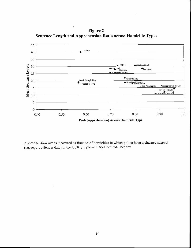
Figure 2Sentence Length and Apprehension Rates across Homicide Types

45 -

40 - — Arson

35 -

30 - • Rape asexual Assault

Aultthetkbb •Burglary

25 - ê Gnnthnd killing

.2 20 - Vn,th r.u ifli Other felony

Narcotics laws • Brawi4c, - Other ArguTnts Arguint over money

Lovers dangle

10 -Brawl un& alcohol

5-

0-0.40 0.50 0.60 0.70 0.80 0.90 1.0

Prob (Apprehension) Across Homicide Type

Apprenhension rate is measured as fraction of homicides in which police have a charged suspect(i.e. report offender data) in the UCR Supplementary Homicide Reports

10

Figure 3Sentence Length and Recidivism Rates across Homicide Types

-l

V

CVCtCV

45

40

35

30

25

20

15

10

5

0

Arson.

•RapeBurglary• • Auto theft

• Ganeland killinoRobbexy•

• Other felony Brawl under drugsYouth Ga

Prostitulton r4k,llin Namotics laws

Other Arguments • • Argument over money

Lover's triangleBrawl under4cohot

0.00 0.05 0.10 0.15 0.20 0.25 0.30 0 .4(0.35

Prob (Recede to Violent) Across Homicide Types

Recidivism rates are fitted values based on offender characteristics. The coefficients for thefitted values are estimated using the BJS data "Recidivism of Felons on Probation."

9