Pathology Severity Coefficient (PSC) Y Pathology Severity ...

Certainty of Punishment versus Severity of Punishment:
An Experimental Investigation
Lana Friesen, School of Economics Discussion Paper No. 400, October 2009, School of Economics, The University of Queensland. Australia.
Full text available as: PDF- Requires Adobe Acrobat Reader or other PDF viewer
Abstract
Compliance with laws and regulations depends on the expected penalty facing violators. The expected penalty
depends on both the probability of punishment and the severity of the punishment if caught. A key question in
the economics of crime literature is whether increasing the probability of punishment is a more effective
deterrent than an equivalent increase in the severity of punishment. This paper uses laboratory experiments to
investigate this issue, and finds that increasing the severity of punishment is a more effective deterrent than an
equivalent increase in the probability of punishment. This result contrasts with the findings of the empirical
crime literature.
EPrint Type: Departmental Technical Report
Keywords: regulatory compliance, experiment, enforcement, penalty
Subjects:
ID Code: JEL Classification: C91, K42, L51, Q58
Deposited By:
Lana Friesen University of Queensland School of Economics Brisbane, QLD 4072 [email protected]
1
Certainty of Punishment versus Severity of Punishment:
An Experimental Investigation
Lana Friesen*
October 2009
Abstract
Compliance with laws and regulations depends on the expected penalty facing violators. The
expected penalty depends on both the probability of punishment and the severity of the
punishment if caught. A key question in the economics of crime literature is whether
increasing the probability of punishment is a more effective deterrent than an equivalent
increase in the severity of punishment. This paper uses laboratory experiments to investigate
this issue, and finds that increasing the severity of punishment is a more effective deterrent
than an equivalent increase in the probability of punishment. This result contrasts with the
findings of the empirical crime literature.
JEL codes: C91, K42, L51, Q58
Keywords: regulatory compliance, experiment, enforcement, penalty
* School of Economics, University of Queensland, Brisbane, Qld 4072, Australia.
Email: [email protected]
2
1. Introduction
Compliance with laws and regulations depends on the expected penalty facing violators. The
expected penalty depends on both the probability of punishment and the severity of the
punishment if caught. A key question in the economics of crime literature is whether
increasing the probability of punishment is a more effective deterrent than an equivalent
increase in the severity of punishment. The answer to this question has implications for the
design of enforcement strategies and, in particular, for the allocation of limited resources.
Should additional resources be devoted to catching violators or to punishing them? This issue
is important not just for policing criminal law, but also for the enforcement of a wide range of
laws and regulations including environmental, occupational health and safety, and traffic
regulations, as well as tax, fraud, and antitrust laws.
The seminal work in the economics of crime and enforcement literature is Becker (1968). In
his model, rational decision makers compare the expected gain from offending with the
expected penalty from offending. Becker (1968) identifies the key role of risk preferences. In
particular, risk neutral individuals consider only the expected penalty and not its composition,
and are therefore indifferent to offsetting changes in the probability and severity of
punishment that keep the expected penalty constant. Risk averse individuals, on the other
hand, are deterred more by (equivalent) increases in severity of punishment, while risk lovers
are deterred more by (equivalent) increases in the probability of detection. Despite the fact
that many extensions have been made to Becker’s (1968) theoretical model (Polinksy and
Shavell, 2000, summarise these developments), the relatively efficacy of violation detection
versus severity remains an unresolved question.
Empirical evidence has largely come from general crime data. The consensus of results from
this literature (summarised by Eide, 2000) supports the general theory of deterrence. That is,
increases in variables such as the probability of detection and conviction, along with
increases in the penalty (either fines or jail terms) tend to reduce crime rates. Comparing the
magnitude of the impacts, increases in the probability of punishment have a larger and more
significant impact than increases in the severity of punishment. The results of these studies
however are often controversial because of the nature of the data used. Data can be either
individual level or at an aggregate (e.g. state) level. Individual level data is either sourced

3
from the criminal justice system, creating sample selection issues (e.g. the data set in
Grogger, 1991, includes only those with a history of past offenses), or based on self-reported
data. If aggregate level data is used, the potential endogeneity of the crime rate and
enforcement parameters, such as the probability of detection, must be accounted for.
Regardless of the type of data, all of these empirical studies have to construct measures of the
probability and severity of punishment that are proxies based on past data, as well as being
estimated without knowledge of the true level of offending. These constructed measures will
also differ from individual perceptions of both the likelihood of being caught and the likely
punishment if arrested.
Because of these data controversies, less credence is given to comparisons of the relative
magnitudes of the effects of increasing probability and severity than to the fact that both have
a negative impact on crime. This leads Polinsky and Shavell (2000, p.73, emphasis added) to
conclude their survey of the economic theory of public enforcement of law with the following
statement: “[e]mpirical work on law enforcement is strongly needed to better measure the
deterrent effects of sanctions, especially to separate the influence of the magnitude of
sanctions from their probability of application.”
Empirical studies on regulatory enforcement are fewer. These studies must also rely on
constructed measures of the key variables, and in the case of environmental enforcement,
penalty information was not available until recent studies. For example, Gray and Deily
(1996) find that enforcement actions increase compliance among steel making plants,
however their analysis includes no data on fines and the enforcement measure is number of
actions taken during the previous two years. Stafford (2002) estimates the impact of an
increase in fines for hazardous waste violations using an indicator variable for pre- and post-
change years. Recent work by Shimshack and Ward (2005) on water pollution includes data
on past penalties and inspections. Using plant level self-reported data, they find that (past)
fines are a more successful deterrent than inspections.1
This paper takes a different approach and uses laboratory experiments to investigate whether
(equivalent) changes in the probability or severity of punishment have a larger impact on
compliance behaviour. The use of a controlled laboratory setting can overcome some of the
1 The inspection measure is the number of inspections at the plant within the last year, while the fine measure is
a dummy variable indicating if any firm was fined in the preceding 12 months.
4
data issues that hamper empirical studies. In particular, individual compliance decisions are
directly observed, and the probability and severity of punishment is varied in a controlled
manner that keeps the expected penalty constant. In addition, the direction of causality is
clear, and individual perceptions of the likelihood of detection and size of potential penalties
are unlikely to deviate substantially from the experimental parameters.
Despite the recent growth of experimental economics as a field, there are only a few
enforcement experiments and even fewer that consider the relative efficacy of probabilities
versus severity of punishment. Experiments on regulatory enforcement more generally are
Clark, Friesen and Muller (2004) and Cason and Gangadharan (2006a); Murphy and
Stranlund (2008) who focus on self-auditing and self-reporting; and Murphy and Stranlund
(2007) and Cason and Gangadharan (2006b) on the enforcement of emissions trading
schemes. Although not the focus of their paper, Murphy and Stranlund (2007) include two
treatments with the same expected penalty, but vary the probability of detection from “low”
to “high”. They find that compliance is unaffected by this change.
To my knowledge, there are only two published economics experiments that focus on the
effects of probability versus severity of punishment.2 Block and Gerety (1995) conduct an
antitrust experiment with a unique subject pool – prisoners – along with a second standard
subject pool of students. They find that students are more responsive to increases in the fine
compared with equivalent increases in the probability of detection, a result consistent with
risk aversion. On the other hand, prisoners respond more to increases in the probability of
detection, a result consistent with being risk lovers. Anderson and Stafford (2003) use a
public goods experiment where free-riding is punished, and find intriguing evidence that
subject contributions respond more to punishment severity than to punishment probability.
While limited in number, these two sets of experimental results involving student subjects
contrast with the findings of the empirical crime literature. One explanation for this
difference is that prisoners, and more generally criminals, are risk lovers, while the typical
student is risk averse. Block and Gerety (1995) provide some evidence in support of this
2 Criminologists Nagin and Pogarsky (2003) also use an experimental approach, but their parameter changes
appear unlikely to reflect equivalent changes in probabilities (described as either “low” or “high”) and penalties
(also described as “high” or “low”). Their results using a student subjects support the findings in the empirical
crime literature.
5
difference, but their measure of risk attitudes (using hypothetical choices) found no
difference between the two subject pools. This paper contributes to this debate using student
subjects and by explicitly measuring both risk preferences and compliance decisions. When
drawing policy implications for regulatory enforcement and other non-violent crimes such as
fraud and traffic violations, student subjects may be the more relevant population to consider.
This paper investigates this contrasting evidence by running experiments that are distinct
from the previous work in the following ways. First, compliance decisions are made in a
simple individual-decision making environment, in contrast to the group decision making
associated with collusion (Block and Gerety, 1995) and public goods contributions (Anderson
and Stafford, 2003). Second, an explicit link is made to theory by measuring subjects’ risk
preference prior to undertaking the compliance decisions. Third, enforcement parameters are
varied in a systematic manner over a range of values motivated by theoretical predictions.
The parameters are varied to ensure that only equivalent changes in probability and severity
of punishment are compared. The main finding is that increases in the severity of punishment
are a more effective deterrent than equivalent increases in the probability of punishment,
which is consistent with risk aversion but distinct from the empirical crime literature.
The paper proceeds as follows. The theoretical framework and predictions are outlined in
Section 2. Section 3 describes the experimental design, with the results presented in Section
4. The conclusion follows in Section 5.
2. Theoretical Model and Predictions
Expected utility theory predicts that risk averse individuals are deterred more by rising
punishments than probabilities, while the opposite is true for risk loving individuals. The
theoretical model is based on Becker (1968).3 An individual (or firm) faces a regulation (e.g.
environmental, health and safety) or law (e.g. speed restriction) that costs $c to comply with.4
Then, with an income (or profit) per period of $y, the individual receives a certain payoff of
y–c if they comply, yielding utility of
3 The many theoretical contributions since Becker (1968) are summarized in Eide (2000) and Polinsky and
Shavell (2000). 4 In Becker’s model, the cost of compliance is the foregone gain from offending.

6
𝐸𝑈 𝑐𝑜𝑚𝑝𝑙𝑦 = 𝑈 𝑦 − 𝑐 . (1)
Alternatively, if they choose not to comply (violate), with probability p they are caught and
subsequently fined $F. The expected utility in the case of violation is:
𝐸𝑈 𝑣𝑖𝑜𝑙𝑎𝑡𝑒 = 𝑝𝑈 𝑦 − 𝐹 + 1 − 𝑝 𝑈(𝑦). (2)
In this simple discrete situation, an individual chooses to violate when (1) > (2), and complies
otherwise. An increase in either p or F reduces (2) and thereby makes it less likely that any
given individual will comply. The key question to be addressed in this paper is whether
increasing p has a larger impact on expected utility, and hence compliance behaviour, than an
equivalent increase in F. As demonstrated by Becker (1968) the answer depends on the risk
preference of the individual. To see this, derive the elasticity of the change in 𝐸𝑈 𝑣𝑖𝑜𝑙𝑎𝑡𝑒
with respect to p 𝜂𝑝 and F 𝜂𝐹 , where both are defined as positive values.
𝜂𝑝 = −
𝑝
𝐸𝑈 𝑈 𝑦 − 𝐹 − 𝑈 𝑦 (3)
𝜂𝐹 =
𝐹
𝐸𝑈𝑝𝑈′ 𝑦 − 𝐹 (4)
Then, 𝜂𝑝 > 𝜂𝐹 , when the following condition holds:
𝑈 𝑦 − 𝑈 𝑦 − 𝐹
𝐹 > 𝑈′ 𝑦 − 𝐹
(5)
This inequality holds when the average rate of change in utility exceeds the marginal rate of
change, which is true when 𝑈′′ 𝑦 > 0 , i.e. when an individual is risk loving. Thus,
increasing the probability of detection (p) has a larger impact on deterrence than an
equivalent increase in the fine (f) for risk loving individuals, while the opposite is true for the
risk averse. Risk neutral individuals are indifferent.
This result can also be demonstrated graphically, as is shown in Figure 1 for the case of a risk
averse individual. An increase in the probability of detection from 𝑝0 to 𝑝1 reduces the
expected utility from violating to 𝐸𝑈(𝑝1𝐹0), but an increase in the fine from 𝐹0 to 𝐹1 causes
7
an even larger reduction in the expected utility from violating to 𝐸𝑈(𝑝0𝐹1), noting that in
both cases the expected fine is the same (𝑝1𝐹0 = 𝑝0𝐹1).
To translate this into predictions regarding the average compliance rate, note that the discrete
nature of the decision results in cases where individuals are (theoretically) unresponsive to
changes in the enforcement parameters. Specifically, if the compliance cost is less than the
expected penalty (c < pF) then both risk averse and risk neutral individuals will always
comply, and when the compliance cost exceeds the expected penalty (c > pF) then both risk
neutral and risk lovers will always violate.5 This leads to the following predictions.
Prediction 1: If c > pF, then an increase in the probability of detection (p) with a
corresponding decrease in the fine (F) such that the expected fine (pF) is unchanged, will
result in a decrease in the average level of compliance.
In this case, we expect no change in the decisions of those who are risk neutral or risk lovers,
while some risk averse individuals will switch from compliance to violation.
Prediction 2: If c < pF, then an increase in the probability of detection (p) with a
corresponding decrease in the fine (F) such that the expected fine (pF) is unchanged, will
result in an increase in the average level of compliance.
In this case we expect no change in the decisions of the risk neutral and risk averse, while
some risk lovers will switch from violation to compliance.
For clarity, these predictions are expressed as definite increases or decreases in the average
level of compliance however a finding of “no change” would also be consistent with theory,
while a change in the opposite direction would be inconsistent. The average level of
compliance would be unchanged if there were few individuals with the required risk
preference or the change in enforcement parameters was too small to induce a change in
behaviour.
5 There is obviously a third case where c = pF and risk averters comply, while risk lovers violate, and the risk
neutral are indifferent. This case is avoided in the experiment because this indifference could generate noise in
the data.
8
3. Experimental Design
The experiment has two parts. In the first part, subjects made a series of ten lottery choices,
which were to estimate their risk preferences. The second part of the experiment involved
subjects making compliance choices in 30 periods, where the enforcement parameters were
varied across the periods to test the predictions outlined above. To avoid confounding
income effects, at the end of the experiment, one decision from part one and one period from
part two were randomly selected to determine subjects’ earnings.6 In addition to their
earnings from the two parts, subjects also received a $5 participation fee.
The experiments were computerized using the programme Z-Tree (Fischbacher, 2007),
however to enhance credibility, physical random devices were used to select the lottery
decision and compliance round that determined earnings. Specifically, a ten-sided die was
used to select one of the ten lottery choices and a bingo cage (containing numbered balls from
one to thirty) was used to choose one compliance period. In each part of the experiment,
subjects received detailed instructions and participated in training exercises prior to
undertaking the real decisions.7
3.1 Lottery Choices
The lottery choice experiment developed by Holt and Laury (2002) was used to estimate
subject’s risk preferences. Subjects made the series of ten lottery choices shown in Table 1,
with these being scaled versions of the choices used by Holt and Laury (2002) with a scaling
factor of five chosen to ensure the range of payoffs is comparable with the payoffs in the
second part of the experiment.8 Subjects choose between a safe option (A) and a risky option
(B), and as they move down the table the probability of the highest payoff increases, until
finally the last decision involves no uncertainty. Subjects choices, and in particular the
lottery at which they switch from choosing A to B, reveals their risk preference.9 Risk
6 The practice of randomly selecting one round or choice for payment is common in lottery choice experiments
where it is crucial to control for income and wealth effects from round to round (see e.g. Hey and Orme, 1994).
Recent experiments support the validity of this procedure (e.g. Cubitt, Starmer and Sugden, 1998; Laury, 2005). 7 A copy of the experimental instructions is available from the author.
8 Payoffs in the scaled up version of the lottery choices ranged from $0.50 - $19.25, while payoffs in the
compliance rounds ranged from $1.00 to $21.00. 9 Consistent subjects should only switch once from A to B, and never back from B to A.

9
neutral individuals should make four safe choices, the risk loving less than four safe choices,
and the risk averse more than four safe choices.
At the end of both parts of the experiment, one of these ten lottery choices was selected at
random using a ten-sided die and played for real according to the subject’s choice and
another roll of a ten-sided die. Subjects were paid accordingly.
3.2 Compliance Choices
In the second part of the experiment, subjects made compliance decisions in 30 periods. In
each round, subjects received a trading (or gross) profit and then faced a choice of whether or
not to comply with a regulation. Compliance incurred a certain cost, while violation incurred
no immediate cost but the possibility of being inspected and subsequently fined. The
compliance cost, probability of inspection, and fine were varied across periods in order to test
the two predictions developed in Section 2.
Specifically, Prediction 1 was tested in 16 periods where c>pF (Set 1), while Prediction 2
was tested in 10 periods where c<pF (Set 2). Within each set, a number of different expected
fine and compliance cost combinations were developed to ensure that the results were not
peculiar to the values chosen. Each combination was used in at least two different periods.
Because previous experimental findings show that most subjects are risk averse (Harrison and
Rutstrom, 2008), more parameters were chosen for Set 1 than for Set 2. The remaining four
periods (Set 3) involved no uncertainty as the inspection probability was either zero or one
and hence all subjects should make the same decision regardless of their risk preference.
These four periods provide a basic check of subject’s decisions. The set of parameter values
was randomly ordered across the 30 periods, with the same order used in all experimental
sessions to enhance comparability.
The choices were framed as general compliance decisions, using the terminology of the
previous paragraphs. One drawback of more “loaded” as opposed to “neutral” language is
that subjects may comply because of perceived social norms or experimenter demand effects
or both. The use of loaded language however is common in income-tax compliance
experiments, and several studies have shown no substantive difference in the results between
neutral and loaded language (Alm, McClelland, and Schulze, 1992; Cason and Gangadharan
10
2006a). In addition, subsequent data analysis (see Section 4.1) checks for these effects and
finds them unlikely.
4. Results
The experiments were held at the University of Queensland during March 2009. There were
139 participants over eight sessions, who earned AUS$30 on average. Payments ranged from
AUS$19.50 - $40.25 and each session lasted between 60-90 minutes. Half of the subjects
were female, the majority were first or second-year students (45% and 35% respectively), and
about one-quarter had never taken an economics or statistics course. Summary statistics are
listed in Table 2 for both demographic variables and constructed outcome measures.
4.1 Risk Aversion and Consistency of Choices
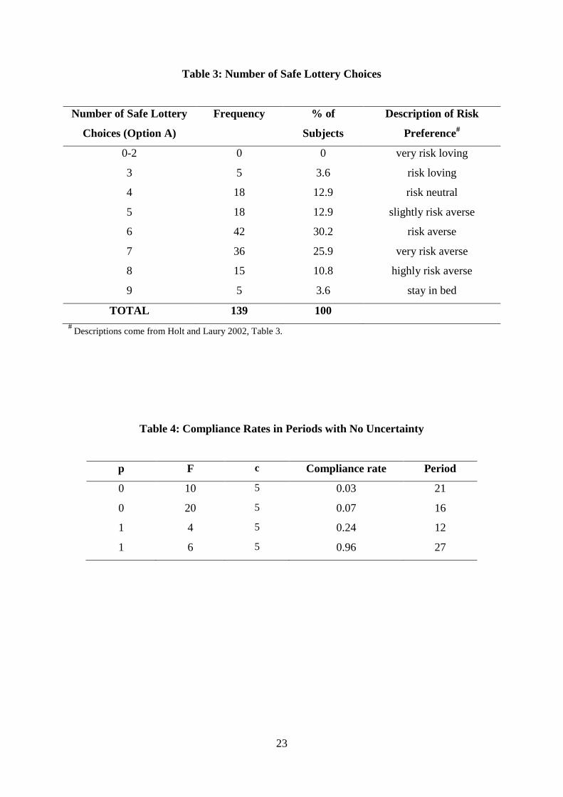
The number of safe lottery choices made by the subjects in part one of the experiment is
summarised in Table 3, which shows that the majority of subjects (83%) are risk averse,
some are risk neutral (13%), and only a few are risk loving (4%).10
These choices can also be
analysed by considering the proportion of safe choices for each decision (rather than for each
individual). This is plotted in Figure 2, which shows that the proportion of safe choices
generally exceeds the risk neutral prediction, suggesting that the majority of subjects are risk
averse. Only nine subjects (6.5%) switched back from Option B to Option A, and only one of
these switched back more than once.11
A further check is that everyone should choose the
safe option in decision 10, which involves no uncertainty. Only one person got this wrong
and it was one of the switchers.
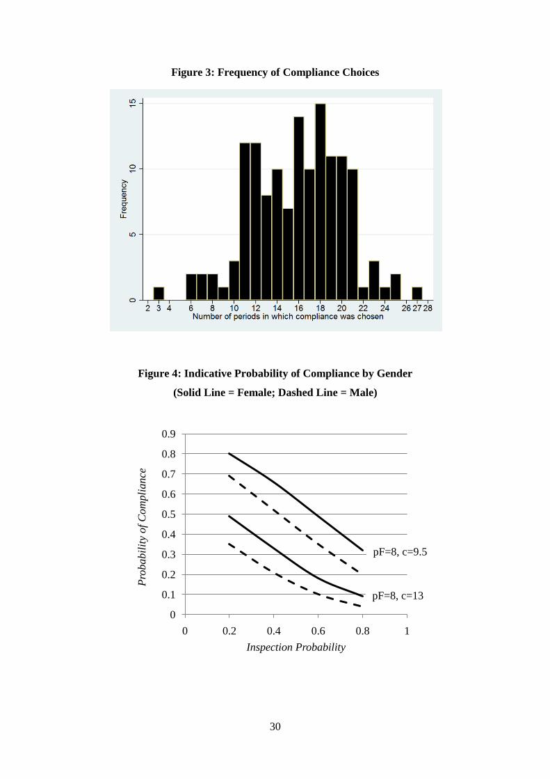
To investigate the potential for experimenter demand effects, the number of periods in which
each subject chose to comply was counted, with Figure 3 showing the frequency of these
compliance choices. None of the 139 subjects chose to either always comply or violate in all
periods. The minimum number of periods complied was 3, the maximum was 27, with the
10
These results are broadly consistent with the existing literature, for example, Holt and Laury (2002, Table 3)
find 8% risk loving (both categories), 26% risk neutral, and 13% very risk averse in their baseline treatments.
Payments here have been scaled up by a factor of five, so greater risk aversion is expected. 11
This rate of switching is comparable to Holt and Laury (2002, p.1648) who find that around 6% of subjects
switched back.

11
majority (86%) choosing to comply in between 11 - 21 periods.12
The fact that no subject
complied in all periods, and in fact very few (6%) complied in more than 21 periods, suggests
that subjects were not complying because they thought they ought to. That is, there is little
evidence that the use of “loaded” terminology generated “experimenter demand” effects.
Decisions of subjects in the four periods without uncertainty (Set 3) give further insights.
The parameter values in these periods and the resulting compliance rates are shown in Table
4. When p=0 everyone should violate and most did. Specifically, in period 16, 10 out of the
139 subjects complied (7%), while in period 21, only four subjects did (3%). Only two
subjects complied in both periods. Subjects however tended to make more errors when p=1
particularly earlier in the experiment. In Period 12, 33 subjects (24%) erroneously chose to
comply, but by period 27 when p=1 only 5 subjects made an erroneous choice. This suggests
that lack of experience may account for many of the errors in Period 12. Indeed, of the 33
subjects who choose comply in Period 12, only six made another error in the experiment.
To further investigate the role of learning as opposed to general error proneness, the number
of errors by subjects is tabulated in Table 5. Subject mistakes are defined as either switching
back in the lottery choice experiment or making the incorrect choice in one of the periods
without uncertainty (Set 3). Of the 139 subjects, 90 (65%) never made a mistake. Of the
remaining 49 subjects, only 10 made more than one mistake as indicated by the shaded cells
in the table.
Before looking at the main research question, consider first whether the results are consistent
with the basic deterrence hypothesis, that is, does increasing either the probability of
inspection or the fine increase compliance, ceteris paribus? Unlike the main analysis where
the expected penalty (pF) is held constant, here pF increases. The results in the Table 6 are
for the 13 periods where the compliance cost (c) was $5 (including Set 3). As you move
down a column or along a row, the expected fine increases, and then if the deterrence
hypothesis holds, the compliance rate should increase. All the changes are in the expected
direction. Using the sign test for matched pairs indicates that all these increases are highly
significant (one-sided p-values = 0.00, except for p=0 when the p-value=0.05).13
12
The subject who complied in only three periods, including one with p=0, was the only subject who switched
twice during the lottery choice part of the experiment. 13
Details of the statistical tests are available from the author.

12
4.2 Univariate Tests
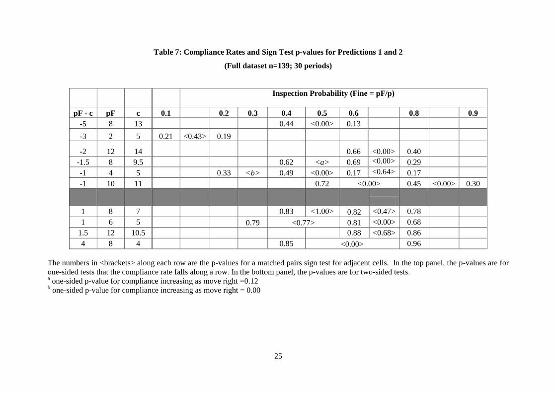
Moving now to the main research question in this paper, the compliance rate in each period is
reported in Table 7 where the data are organised so that along each row in the table both the
expected fine and compliance cost are constant. The top panel reports results from Set 1
where c > pF and according to Prediction 1, as we move right along each row the compliance
rate should fall. The bottom panel reports results from Set 2 where c < pF and if Prediction 2
is correct, as we move right along each row the compliance rate should increase. The
numbers in <brackets> are the p-values from the sign test for matched pairs for adjacent cells
along the row. For Set 1 these are one-sided tests, but for Set 2 two-sided tests are used
because no directional pattern was obvious from the data.
Of the ten pair wise comparisons in the top panel (Set 1) six show compliance significantly
falling as p increases holding pF constant (p-value=0.00, one-sided), two show no significant
change, and two show compliance actually increasing (p-values=0.00 and 0.12, one-sided).
Of the six pair wise comparisons in the bottom panel (Set 2), four show no change, while one
shows a significant increase in compliance (bottom row) and another a significant decrease
(second row). Since the results of the lottery choice experiment indicate that few subjects are
risk lovers it is not surprising to find no effect being common in Set 2. Similarly, a result of
no change in Set 1 is not evidence against Prediction 1 as it may simply be that the changes
are not sufficient to cause a change in behaviour.
To check how many of these anomalous results were due to error-prone individuals, the tests
in Table 7 were recalculated using only the compliance decisions for the 90 individuals who
never made an error. This reduces but does not eliminate the anomalous results. In
particular, in Set 1 there are still six pair wise comparisons that are significant decreases, but
now three results of no change, and only one remaining wrong direction (p-value=0.08, one-
sided) in row 5. For Set 2, there are five results of no change, but still one wrong direction in
row 2 (p-value=0.01, two-sided).14
This suggests that error-prone individuals may have
resulted in some, but not all of these anomalous results.
14
Detailed results are available from the author.
13
4.3 Panel Data Regression Analysis
While the results from the univariate tests generally support Prediction 1 they do not control
for demographic factors and possible learning over the periods. The following section
rectifies this by estimating a random effects probit model of compliance choices. The dataset
is a panel with 30 compliance decisions for each of the 139 subjects, and a binary dependent
variable indicating whether the subject chose to comply in a particular period.
The model can be motivated as a latent variable model where the latent index y* is
𝐸𝑈 𝑐𝑜𝑚𝑝𝑙𝑦 − 𝐸𝑈(𝑣𝑖𝑜𝑙𝑎𝑡𝑒) , which is modelled as 𝑦𝑖𝑡∗ = 𝑋𝑖𝑡𝛽 + 𝛼𝑖 + 𝜀𝑖𝑡 , where 𝛼𝑖 is
unobserved individual heterogeneity and 𝜀𝑖𝑡 is the usual idiosyncratic error term. In this
model compliance occurs (𝑦𝑖𝑡 = 1) if 𝑦𝑖𝑡∗ >0, otherwise violation occurs (𝑦𝑖𝑡 = 0). The
explanatory variables fall into three categories: enforcement variables, demographic
variables, and experimental control variables.
The empirical strategy used to test the predictions excludes Fine as a separate explanatory
variable because it does not change independently of the Inspection Probability and the
Expected Fine. A negative estimated coefficient on the variable Inspection Probability is
then evidence in favour of Prediction 1. That is, as the inspection probability increases,
ceteris paribus (which means in this case that pF is unchanged, so F is adjusted down), the
compliance rate falls.15
Along with standard demographic variables (e.g. gender, age), the number of safe lottery
choices from the first part of the experiment is also included to measure risk preferences.
The experimental control variables include session dummies, and a time trend (Period), to
account for any learning or timing effect that occurred even though the order of parameters
was predetermined in a random manner.
The model is estimated separately for the two sets of parameters, with the results for Set 1
(c>pF) reported in panel A of Table 8 and for Set 2 (c<pF) in panel B of Table 8.16
In the
15
Block and Gerety (1995) use a similar approach but do not have panel data. 16
Estimating the model using the entire dataset of 30 periods yields qualitatively similar results to Set 1. That
is, the coefficient on inspection probability is significantly negative, however the marginal effect is less than
half of that reported in Table 9.
14
first column any relevant periods from Set 3 are also included (All Periods) while the second
and third columns only use periods where 0 < 𝑝 < 1 (Interior), and in the right column only
the 90 subjects without errors are included (No Error).
Consider first the most general model (All Periods) for Set 1, which includes all the
demographic variables as well as dummy variables for each session. All the treatment
variables have the correct sign and are highly significant. The coefficient on Inspection
Probability is significantly negative providing support for Prediction 1. Of the demographic
variables, only gender and number of safe choices significantly affect the probability of
compliance. Females subjects are more likely to comply than similar male subjects, and
those who made a greater number of safe lottery choices are also more likely to comply.
Subjects are also more likely to comply in later periods.17
Restricting the data to only those
periods with 0 < 𝑝 < 1 (Interior I) does not qualitatively change any of the results. When
the observations are limited to only the 90 subjects who made no errors (No Error), the effect
of Period becomes more statistically significant and fourth year students are more likely to
comply, ceteris paribus. In all three models, the coefficient on Inspection Probability
remains negative providing robust evidence in support of Prediction 1.
To facilitate computation of the marginal effects, the model is estimated (Interior II)
excluding the insignificant demographic variables, all but one of which is an indicator
variable, and the session variables. Table 9 reports the marginal effects at the average
treatment values, with the random effect equal to zero. The gender effect is large, with
females having a 13.3% higher probability of compliance than males with the same risk
preference. In terms of magnitudes, a 1% increase in the probability of inspection decreases
the probability of compliance by slightly less than 1%.18
The impact of changes in the
expected fine and compliance cost are larger. The Period effect, while statistically
significant, is small in magnitude with each additional period increasing the probability of
compliance by only 0.3%. Gender does not substantially change the marginal effects
although females appear slightly more responsive to the parameter changes than males.
17
Very few of the session dummies are significant and none consistently so across all the models. 18
The marginal effect of Inspection Probability at average treatment values is slightly higher in the No Error
model at 1.2% for females and 1.0% for males.
15
With this non-linear estimation method, the magnitude of these marginal effects depends on
the parameters at which they are evaluated. Some indicative values are shown in Figure 4,
where in the top case both the gender effect and marginal effect of inspections are constant
throughout the range of values illustrated. In the bottom case however, both the marginal
effect of inspections and the gender effect become smaller as the inspection probability
increases and the compliance probability falls to a low level.
In addition to providing robust evidence in support of Prediction 1, two auxiliary conclusions
are also worth mentioning. The first regards the predictive value of the Holt and Laury
(2002) lottery choice measure of risk preference. In all versions of the model, the number of
safe lottery choices made in part one of the experiment had a highly significant positive
relationship with the probability of compliance in part two of the experiment. A positive
coefficient is expected because compliance is a riskless choice, while you face uncertainty if
you choose violation.
The second result is the substantial gender effect where (at average treatment values) females
are 13% more likely to comply than males. This effect is robust across all versions of the
model. This difference applies to “otherwise identical” female and male participants, so even
though female participants were significantly more risk averse (average number of safe
lottery choices = 6.4) than male participants (average = 5.8, Mann-Whitney two-sided p-
value=0.0054), this cannot explain the gender effect.19
Instead, the explanation may lie in
different preferences or social conditioning, as other studies have found a similar effect. For
example, Nagin and Pogarsky (2003, p. 179) found that men were 10% more likely to cheat,
which they note is “[c]onsistent with virtually all work relating gender to offending.” Within
economics, gender differences in social preferences and competitive inclinations have been
studied (see the recent review by Croson and Gneezy, 2009) but are rarely considered in
compliance experiments.20
Table 8B presents the results for Set 2, with the models defined in the same way as for Set 1.
The results are sensitive to the dataset used, with consistent effects across the models found
only for Expected Fine (positive), Compliance Cost (negative), and Number of Safe Lottery
19
This is consistent with a robust finding in the literature than women are more risk averse than men (Croson
and Gneezy 2009). 20
One exception is Anderson and Stafford (2003) who found that gender was an insignificant determinant of
group contributions in their public goods experiment.
16
Choices (positive). A positive coefficient on Inspection Probability is evidence in support of
Prediction 2, but only occurs in the All Periods model. The All Periods model includes not
only the 10 periods of Set 2, but also Period 27 from Set 3 where p=1, c=5, F=6 and all
except five subjects complied. When data from Period 27 are excluded, as in Interior I, the
coefficient becomes insignificant, suggesting that the positive coefficient is strongly
influenced by the results from this one period. Interestingly when only error-free subjects are
included (No Error), the coefficient becomes significantly negative. The direction of the
change is consistent with risk averse behaviour, although theoretically, risk averse individuals
should always comply when c<pF. I conjecture, but do not formally test, that this is due to
decision-making errors, so that while the risk averse do not match the point predictions of
expected utility theory exactly, they are consistent with the comparative static predictions. It
is also interesting to note that when Period 27 is excluded from the data, the Period effect
disappears. As for the demographic variables, there is no gender effect in Set 2, but having
taken a statistics course increases your chance of compliance in most models. The Number of
Safe Lottery Choices continues to have a significant positive relationship with compliance.
The evidence with regard to Prediction 2 is therefore mixed and dependent on the model
estimated. This conclusion is not surprising given that only five (3.6%) of the subjects were
risk loving in the lottery choice task.
5. Discussion
The main result of this paper is that increasing the severity of punishment is a more effective
deterrent than an equivalent increase in the probability of punishment. The lottery choice
task indicates that most subjects are risk averse, and the aggregate responses in the
compliance task are theoretically consistent with this. Indeed the number of safe lottery
choices was a strong predictor of compliance behaviour. While these results strongly contrast
with those in the empirical crime literature, where increases in the probability of punishment
have a larger and more significant impact on deterring crime than increases in the penalty,
they are consistent with the limited amount of existing experimental evidence involving
student subjects.
Two broad factors can account for the different results between the empirical and
experimental literature. The first difference is the methodology, with each approach having

17
(different) limitations. As discussed in Section 1, the empirical crime literature faces issues
of sample selection, the possible endogeneity of crime and enforcement, and the use of
constructed measures of probabilities and penalties that are likely to differ from individual
perceptions of these parameters. The use of laboratory experiments overcomes these data
issues, but in doing so abstracts from real world context such as social norms and non-
monetary punishments such as shame and prison sentences, which also affect deterrence.
Both methods therefore have limitations, and it is not clear a priori which is necessarily more
informative.
The second point of difference is the subject pool, with the empirical crime literature
typically using data from criminals, while laboratory experiments typically involve students.
While the results of Block and Gerety (1995) suggest the two subject pools behave in
different ways, this has yet to be replicated in other studies. On the other hand, students will
be a more appropriate subject pool for many types of non-violent crime (e.g. traffic offences,
fraud, false advertising) and for regulatory compliance decisions, as they will often progress
into the managerial positions responsible for these decisions. Experimental results may be of
particular help in designing regulatory enforcement schemes where empirical data is often
scarce.
These results suggest that regulatory enforcers should focus more on increasing the severity
of punishment than on increasing the probability of detection. This is good news for
regulators facing a limited enforcement budget, as the cost of imposing (monetary)
punishments is typically less than the cost of catching violators. On the other hand, designing
the optimal enforcement scheme requires considerations of justice, marginal deterrence, and
practical upper limits on wealth, which may limit the maximum penalty.
Of the auxiliary results, the strong gender effect is intriguing. Croson and Gneezy (2009)
propose that female social preferences are more amenable to changes in the (experimental)
context, and it will be interesting to see if this effect holds in other similar experiments.
Along with testing for a gender effect, future compliance experiments could use a more
diverse subject pool.
18
References
Alm, James, McClelland, Gary H., and Schulze, William D. (1992), "Why Do People Pay
Taxes?" Journal of Public Economics, 48, 21-38.
Anderson, Lisa R. and Sarah L. Stafford (2003) "Punishment in a Regulatory Setting:
Experimental Evidence from the VCM", Journal of Regulatory Economics, 24(1), 91-110.
Becker, Gary S. (1968) "Crime and punishment: An economic approach", Journal of
Political Economy, 76, 169-217.
Block, Michael K. and Vernon E. Gerety (1995) "Some experimental evidence on differences
between student and prisoner reactions to monetary penalties and risk", Journal of Legal
Studies, 24, 123-38.
Cason, Timothy N. and Lata Gangadharan (2006a). "An experimental study of compliance
and leverage in auditing and regulatory enforcement", Economic Inquiry, 44(2), 352-66.
Cason, Timothy N. and Gangadharan, Lata (2006b), "Emissions Variability in Tradable
Permit Markets with Imperfect Enforcement and Banking", Journal of Economic Behavior &
Organization, 61(2), 199-216.
Clark, Jeremy, Friesen, Lana and Andrew Muller (2004), “The Good, the Bad, and the
Regulator: An Experimental Test of Two Conditional Audit Schemes”, Economic Inquiry 42,
69-87.
Croson, Rachel and Uri Gneezy (2009), "Gender Differences in Preferences," Journal of
Economic Literature, 47, 1-27.
Cubitt, Robin P., Starmer, Chris, and Sugden, Robert (1998), "On the Validity of the Random
Lottery Incentive System," Experimental Economics, 1, 115-131.
19
Eide, Erling (2000), Economics of criminal behavior, in Encyclopedia of Law and
Economics, Boudewijn Bouckaert and Gerrit De Geest (eds), Cheltenham: Edward Elgar.
Fischbacher, Urs (2007), "Z-Tree: Zurich Toolbox for Ready-Made Economic Experiments",
Experimental Economics, 10, 171-78.
Gray, Wayne B., and Mary E. Deily (1996), "Compliance and Enforcement: Air Pollution
Regulation in the U.S. Steel Industry," Journal of Environmental Economics and
Management, 31, 96-111.
Grogger, Jeffrey (1991), "Certainty vs. Severity of Punishment", Economic Inquiry, 29(2),
297-309.
Harrison, Glenn W. and E. Elisabet Rutstrom (2008), Risk Aversion in the Laboratory, in
Risk Aversion in Experiments, James C. Cox and Glenn W. Harrison (eds), JAI Press.
Hey, John D. and Chris Orme (1994), “Investigating generalizations of expected utility
theory using experimental data”, Econometrica, 62(6), 1291-1326.
Holt, Charles A and Susan K Laury (2002), "Risk aversion and incentive effects", American
Economic Review, 92(5), 1644-55.
Laury, Susan (2005), "Pay One or Pay All: Random Selection of One Choice for Payment",
SSRN Working Paper.
Murphy, James J. and John K. Stranlund (2008), An Investigation of Voluntary Discovery
and Disclosure of Environmental Regulations Using Laboratory Experiments, in
Environmental Economics, Experimental Methods, T. L. Cherry, S. Kroll and J. F. Shogren
(eds), London: Routledge.
Murphy, James J. and John K. Stranlund (2007), "A laboratory investigation of compliance
behavior under tradable emissions rights: Implications for targeted enforcement", Journal of
Environmental Economics and Management, 53(2), 196-212.
20
Nagin, Daniel S., and Greg Pogarsky (2003), "An Experimental Investigation of Deterrence:
Cheating, Self-Serving Bias, and Impulsivity," Criminology, 41, 167-194.
Polinsky, A. Mitchell and Steven Shavell (2000), "The economic theory of public
enforcement of law", Journal of Economic Literature, 38(1), 45-76.
Shimshack, Jay P., and Michael B. Ward, (2005), "Regulator Reputation, Enforcement, and
Environmental Compliance," Journal of Environmental Economics and Management, 50,
519-540.
Stafford, Sarah L. (2002), "The Effect of Punishment on Firm Compliance with Hazardous
Waste Regulations," Journal of Environmental Economics and Management, 44, 290-308.

21
Table 1: Lottery Choices
Decision Option A Option B Your Choice
1st $10.00 if the die is 1
$8.00 if the die is 2 - 10
$19.25 if the die is 1
$0.50 if the die is 2 - 10 A: or B:
2nd $10.00 if the die is 1-2
$8.00 if the die is 3 - 10
$19.25 if the die is 1-2
$0.50 if the die is 3 - 10 A: or B:
3rd $10.00 if the die is 1-3
$8.00 if the die is 4 - 10
$19.25 if the die is 1-3
$0.50 if the die is 4 - 10 A: or B:
… …
9th $10.00 if the die is 1 - 9
$8.00 if the die is 10
$19.25 if the die is 1 - 9
$0.50 if the die is 10 A: or B:
10th $10.00 if the die is 1 – 10 $19.25 if the die is 1 – 10 A: or B:

22
Table 2: Summary Statistics
Variable Description Mean Std Dev Minimum Maximum n
Demographic Variables
Age (years) 20.19 3.29 17 42 139
Female 0.50 0.50 0 1 139
First year student 0.45 0.50 0 1 139
Second year student 0.35 0.48 0 1 139
Third year student 0.12 0.32 0 1 139
Fourth year or higher 0.09 0.28 0 1 139
Taken econ course 0.78 0.41 0 1 139
Taken stats course 0.75 0.44 0 1 139
Treatment Variables
Inspection prob (%) 56 27.99 0 100 30
Fine 13.76 5.45 4 20 30
Expected fine 6.87 3.39 0 12 30
Compliance cost 7.68 3.31 4 14 30
Outcome Variables by Subject
Number of periods of
compliance (0-30)
15.86 4.30 3 27 139
Number of safe lottery
choices (0-10)
6.09 1.41 3 9 139
Outcome Variables by Round
Compliance rate (%) 52.73 29.72 3 96 30
23
Table 3: Number of Safe Lottery Choices
Number of Safe Lottery
Choices (Option A)
Frequency % of
Subjects
Description of Risk
Preference#
0-2 0 0 very risk loving
3 5 3.6 risk loving
4 18 12.9 risk neutral
5 18 12.9 slightly risk averse
6 42 30.2 risk averse
7 36 25.9 very risk averse
8 15 10.8 highly risk averse
9 5 3.6 stay in bed
TOTAL 139 100
# Descriptions come from Holt and Laury 2002, Table 3.
Table 4: Compliance Rates in Periods with No Uncertainty
p F c Compliance rate Period
0 10 5 0.03 21
0 20 5 0.07 16
1 4 5 0.24 12
1 6 5 0.96 27

24
Table 5: Number of Errors made by Subjects
Number of errors in periods with no
uncertainty
0 1 2 3 Total
Switch back in lottery 4 4* 1 0 9
No switch back in lottery 90 35 4 1 130
Total 94 39 5 1 139
* one of these subjects switched twice in the lottery
Table 6: Compliance Rates in Periods with c=5
Inspection Probability
FINE 0 0.1 0.2 0.3 0.4 0.6 0.8 1
4
0.24
5
0.17
6
0.96*
6.67
0.17
7.50
0.68*
10 0.03
0.19
0.49 0.81*
20 0.07 0.21 0.33 0.79*
* indicates that pF>c so both risk averse and risk neutral individuals should comply
25
Table 7: Compliance Rates and Sign Test p-values for Predictions 1 and 2
(Full dataset n=139; 30 periods)
Inspection Probability (Fine = pF/p)
pF - c pF c 0.1
0.2 0.3 0.4 0.5 0.6 0.8
0.9
-5 8 13
0.44 <0.00> 0.13
-3 2 5 0.21 <0.43> 0.19
-2 12 14
0.66 <0.00> 0.40
-1.5 8 9.5
0.62 <a>
0.69 <0.00> 0.29
-1 4 5
0.33 <b> 0.49 <0.00> 0.17 <0.64> 0.17
-1 10 11
0.72 <0.00> 0.45 <0.00> 0.30
1 8 7
0.83 <1.00> 0.82 <0.47> 0.78
1 6 5
0.79 <0.77> 0.81 <0.00> 0.68
1.5 12 10.5
0.88 <0.68> 0.86
4 8 4
0.85 <0.00> 0.96
The numbers in <brackets> along each row are the p-values for a matched pairs sign test for adjacent cells. In the top panel, the p-values are for
one-sided tests that the compliance rate falls along a row. In the bottom panel, the p-values are for two-sided tests. a one-sided p-value for compliance increasing as move right =0.12
b one-sided p-value for compliance increasing as move right = 0.00

Table 8A: Probit Random Effects Results – SET 1
DEPENDENT VARIABLE: Comply = 1, Violate = 0
All Periods Interior I Interior II No Error
Inspection Probability -0.0152***
(0.0015)
-0.0222***
(0.0019)
-0.0222***
(0.0019)
-0.0333***
(0.0026)
Expected Fine 0.4355***
(0.0273)
0.4605***
(0.0333)
0.4607***
(0.0333)
0.5577***
(0.0443)
Compliance Cost -0.2572***
(0.0238)
-0.2482***
(0.0266)
-0.2481***
(0.0266)
-0.3001***
(0.0345)
Period 0.0057*
(0.0033)
0.0077**
(0.0035)
0.0077**
(0.0035)
0.0131***
(0.0046)
Age -0.0037
(0.0160)
-0.0018
(0.0167)
-0.0077
(0.0183)
Female 0.3782***
(0.1015)
0.4244***
(0.1066)
0.3594***
(0.1061)
0.4387***
(0.1195)
Number of Safe Lottery
Choices
0.1487***
(0.0352)
0.1747***
(0.0373)
0.1852***
(0.0383)
0.2192***
(0.0464)
Econ Course -0.1416
(0.1298)
-0.1411
(0.1364)
-0.1730
(0.1582)
Stats Course
0.1678
(0.1277)
0.2192
(0.1343)
0.2618
(0.1637)
Second Year -0.0270
(0.1145)
-0.0394
(0.1204)
-0.0448
(0.1386)
Third Year -0.1543
(0.1628)
-0.1500
(0.1705)
-0.1034
(0.1881)
Fourth Year 0.1530
(0.1830)
0.1698
(0.1922)
0.5949***
(0.2028)
Constant -1.5071***
(0.4296)
-1.6542***
(0.4520)
-1.6183***
(0.2605)
-1.6385***
(0.5400)
Session Dummies Yes Yes No Yes
Observations 2641 2224 2224 1440
Number of periods 19 16 16 16
Number of subjects 139 139 139 90
Log likelihood -1389.77 -1238.53 -1248.88 -739.45
Prob > Chi-squareda 0.0000 0.0000 0.0000 0.0000
*, **, *** indicate significance at the 10%, 5% and 1% levels, respectively. Numbers in parentheses are
standard errors. Estimated using Stata 10.1. a Result of Wald test of model significance, degrees of freedom equal number of regressors (excluding
constant).

27
Table 8B: Probit Random Effects Results – SET 2
DEPENDENT VARIABLE: Comply = 1, Violate = 0
All Periods Interior I Interior II No Error
Inspection Probability 0.0046**
(0.0022)
-0.0011
(0.0025)
-0.0013
(0.0025)
-0.0099***
(0.0033)
Expected Fine 0.1884***
(0.0450)
0.2593***
(0.0470)
0.2585***
(0.0454)
0.4116***
(0.0739)
Compliance Cost -0.1371***
(0.0461)
-0.1841***
(0.0466)
-0.1829***
(0.0434)
-0.3202***
(0.0757)
Period 0.0128**
(0.0058)
-0.0005
(0.0064)
0.0135
(0.0089)
Age 0.0166
(0.0205)
0.0187
(0.0216)
0.0294
(0.0272)
Female 0.0576
(0.1303)
0.0753
(0.1382)
0.0209
(0.1846)
Number of Safe Lottery
Choices
0.1333***
(0.0457)
0.1537***
(0.0486)
0.1585***
(0.0484)
0.2125***
(0.0736)
Econ Course -0.0467
(0.1677)
-0.0892
(0.1792)
0.0673
(0.2397)
Stats Course
0.3990**
(0.1632)
0.4152**
(0.1740)
0.3493**
(0.1499)
0.3823
(0.2443)
Second Year -0.1171
(0.1501)
-0.0928
(0.1593)
-0.1212
(0.2412)
Third Year -0.1374
(0.2092)
-0.1094
(0.2220)
-0.1553
(0.2875)
Fourth Year 0.3118
(0.2634)
0.3382
(0.2772)
0.4690
(0.3658)
Constant -1.3676**
(0.5750)
-1.3355**
(0.6104)
-0.9338**
(0.3831)
-1.7822**
(0.8455)
Session Dummies Yes Yes No Yes
Observations 1529 1390 1390 900
Number of periods 11 10 10 10
Number of subjects 139 139 139 90
Log likelihood -611.82 -574.71 -581.64 -333.48
Prob > Chi-squareda 0.0000 0.0000 0.0000 0.0000
*, **, *** indicate significance at the 10%, 5% and 1% levels, respectively. Numbers in parentheses are
standard errors. Estimated using Stata 10.1. a Result of Wald test of model significance, degrees of freedom equal number of regressors (excluding
constant).

28
Table 9: Marginal Effects at Average Treatment Values
FEMALE
Marginal Effect
MALE
Marginal Effect
Evaluated at
PROBABILITY COMPLY 0.4222
0.2892
Inspection Probability -0.0087 -0.0076 54
Expected Fine 0.1803 0.1575 7
Compliance Cost -0.0971 -0.0848 9
Period 0.0030 0.0026 15
Number of Safe Lottery Choices 0.0725 0.0633 6

29
Figure 1: Risk averse individuals are deterred more by an increase in the fine than an
equivalent increase in the probability of detection.
Figure 2: Proportion of safe choices by decision
0
0.1
0.2
0.3
0.4
0.5
0.6
0.7
0.8
0.9
1
1 2 3 4 5 6 7 8 9 10
Pro
port
ion
of
Safe
C
hoic
es
Decision
Proportion of SAFE
choices
Risk neutral
prediction
EU(p0F0)
Utility
U(y)
EU(p1F0)
EU(p0F1)
y y-F1 y-F0 y-p1F0
=y-p0F1
Income y-p0F0
30
Figure 3: Frequency of Compliance Choices
Figure 4: Indicative Probability of Compliance by Gender
(Solid Line = Female; Dashed Line = Male)
0
0.1
0.2
0.3
0.4
0.5
0.6
0.7
0.8
0.9
0 0.2 0.4 0.6 0.8 1
Pro
babil
ity
of
Com
pli
ance
Inspection Probability
pF=8, c=9.5
pF=8, c=13