Certainty of Punishment versus Severity of Punishment:Deterrence and the Crowding Out of Intrinsic Motivation

Dietrich Earnhart *Department of Economics

University of Kansas

Lana FriesenSchool of Economics

University of Queensland

September 24, 2014

Disclaimer: This manuscript was partially developed under a STAR Research Assistance Agreement No. R-82882801-0 awarded by the U.S. Environmental Protection Agency. It has not been formally reviewedby the EPA. The views expressed in this document are solely those of the authors. The EPA does notendorse any products or commercial services mentioned in this manuscript.

Acknowledgments: We thank Dylan Rassier and Trisha Shrum for their excellent research assistance. Wealso thank the University of Queensland for their financial support of our collaboration.

* Corresponding Author’s Contact Information:Dietrich EarnhartDepartment of Economics; University of Kansas435 Snow Hall; Lawrence, KS 66045Phone: 785-864-2866Email: Earnhart@ku.edu

1

Certainty of Punishment versus Severity of Punishment:Deterrence and the Crowding Out of Intrinsic Motivation

Abstract: According to standard theory, deterrence generated by enforcement stems from two

components of expected penalty imposition: likelihood and size. Penalty likelihood reflects the

certainty of punishment; penalty size reflects the severity of punishment. While standard theory

predicts the relative efficacy of punishment certainty versus punishment severity in deterring crime

risk, the empirical and experimental evidence is mixed. Our study represents the first attempt to

compare systematically the effects of punishment certainty and severity in the environmental

compliance context. In addition to standard deterrence factors, we also importantly consider the role

of intrinsic motivation by allowing for the possibility that explicit monetary incentives might crowd

out the intrinsic motivation to comply, particularly when the monetary incentives are small. As part

of this consideration, we allow the marginal effects of punishment certainty and severity to vary with

the values of the enforcement components; consequently, these effects may become counter-

productive over a range of enforcement values. As another contribution, we employ theoretically

motivated measures of likelihood and severity based on the presence of actually imposed sanctions.

Our empirical analysis makes these contributions by examining wastewater discharged by chemical

manufacturing facilities permitted within the Clean Water Act’s National Pollutant Discharge

Elimination System between 1995 and 2001. We find evidence that increasing either certainty or

severity can be counter-productive when enforcement is weak. In contrast, when enforcement is

high, both components are effective at deterring pollution, although certainty is more effective. For

intermediate values, the results are more mixed. These results highlight the importance of allowing

the estimated marginal effects to vary with the values of the enforcement components.

JEL Codes: K32, K42, Q53

2

1. Introduction

According to the standard model of enforcement (Becker, 1968; Polinsky and Shavell, 2000),

deterrence stemming from the enforcement of laws, including both criminal law and regulations

imposed on businesses, is based on two components of expected penalty imposition: likelihood and

size. The likelihood of a penalty reflects the certainty of punishment; the size of a penalty reflects

the severity of punishment. Crimes are committed or regulations violated when the expected gain

from offending exceeds the expected penalty from offending. Potential offenders are rational

economic agents with full knowledge of the enforcement regime; in particular, they know the

likelihood and severity of punishment before potentially committing a crime.

The standard model predicts that increases in either the probability of punishment or the size

of the penalty (either fines or jail terms) reduce offenses, known as the general theory of deterrence.

This prediction has been borne out in numerous empirical studies of both general crime (Eide, 2000;

Eide et al., 2006) and regulatory compliance (Gray and Shimshack, 2011). The standard model also

predicts the relative efficacy of punishment certainty versus severity in deterring crime based on risk

preferences. Here the evidence is more mixed with empirical results from general crime data

suggesting that increases in the probability of punishment have a larger and more significant impact

than increases in the severity of punishment (Grogger, 1991; Eide, 2000), while experimental studies

find the opposite (Anderson and Stafford, 2003; Friesen, 2012). While several empirical studies of

regulatory compliance separately estimate the effects of certainty and severity (Scholz and Gray,

1990; Sigman, 1998; Shimshack and Ward, 2005), none formally compares the two effects. Our1

study thus represents the first attempt to compare systematically the effects of punishment certainty

and severity in the environmental compliance context. A better understanding of this point is

Scholz and Gray (1990) examine enforcement of occupational safety and health regulations.1

Sigman (1998) studies the illegal dumping of waste material. Shimshack and Ward (2005) study waterpollution from the pulp and paper industry.

3

important for policy considerations since enforcement agencies should place greater emphasis on the

more effective lever – certainty of punishment or severity of punishment.

In the standard model, however, deterrence depends exclusively on explicit monetary

disincentives or extrinsic motivation. Yet, the manager of a regulated firm may also be motivated

intrinsically by a desire to obey the law or cooperate with regulators. Substantial literature shows

that explicit monetary incentives can often crowd out these intrinsic motivations, particularly when

the monetary incentives are small (Frey and Jegen, 2001; Fehr and Falk, 2002; Gneezy et al., 2011).

In the environmental context, explicit threats (Short and Toffel, 2010) and coercive enforcement

styles (Winter and May, 2001; Earnhart and Glicksman, 2013) are shown to reduce compliance.2

Therefore, simply increasing penalties or explicit threats to impose penalties may not enhance

deterrence particularly when the monetary incentives are small. Two opposing effects operate: the

standard deterrence effect and the crowding out effect. The literature suggests that the deterrence

effect should dominate when the monetary incentives are large, while the crowding out effect may

dominate when the monetary incentives are small, even to the extent of causing greater enforcement

to become counter-productive in this range. In the intermediate range, while greater enforcement

still enhances deterrence overall, the effect may be partially offset by the crowding out effect. Thus,

the efficacy of enforcement instruments is not constant but varies with the monetary incentives; as

important, which effect dominates and under which conditions remains an empirical question.

As our second contribution, we allow the effects of certainty and severity to vary with the

size of the enforcement threat by incorporating an interaction term between the two enforcement

components, i.e., the marginal effect of each enforcement component depends on the strength of the

other component. This incorporation allows for countervailing forces to matter (potentially) in a way

In addition to the studies cited above, which demonstrate how penalties can be counter-productive,2

Helland and Whitford (2003) and Gray and Shadbegian (2004) find that greater inspection-related generaldeterrence appears to increase certain categories of emissions.

4

that is not possible in standard empirical approaches that assume constant deterrence effects. We

further enhance this contribution by extending the standard deterrence framework to include intrinsic

compliance motivations. This extension provides theoretical support for our empirical approach,

as well as providing a framework for interpreting our results.

As our third contribution, we carefully construct the measure of sanction likelihood in a

manner consistent with theory. Specifically, our study measures the likelihood of punishment based

on the presence of sanctions, as compared with presence of inspections, as well as computing

sanction severity conditional on a sanction being imposed. In contrast, most other empirical studies

of regulatory compliance examine only the monetary value of punishment, which represents the

product of the likelihood and severity of punishment (Earnhart, 2004a; Earnhart, 2009). As the two

closest studies, Sigman (1998) uses inspections as her proxy for enforcement certainty and the state-

level maximum criminal fine as her proxy for enforcement severity, a measure which even the author

acknowledges may not be ideal especially since the study does not allow the measure to vary over

the sample period. Similar to Sigman (1998), Shimshack and Ward (2005) use inspections as their

proxy for enforcement certainty; in contrast, the authors use the monetary value of fines as their

proxy for enforcement severity, which mixes the two enforcement components – certainty and

severity.

Finally, our study captures both specific and general deterrence. Specific deterrence concerns

the effect of increased monitoring or enforcement against an individual regulated facility on this

same facility’s subsequent compliance decisions; general deterrence concerns the effect of increased

monitoring or enforcement against other regulated facilities on the individual facility’s subsequent

compliance decisions. The evidence of enforcement-based specific deterrence is rather mixed.

While one study provides evidence of specific deterrence (Earnhart, 2004b), other studies provide

only mixed evidence (Foulon et al., 2002) or no evidence (Eckert, 2004; Shimshack and Ward,

5

2005). Most important, no study of industrial polluters finds evidence of specific deterrence when

the analysis also controls for general deterrence. Indeed, few studies explicitly scrutinize specific

deterrence within a broader context of deterrence (Earnhart, 2004a; Shimshack and Ward, 2005).

We not only control for both types of deterrence but also estimate the relative effects of certainty and

severity for both general and specific deterrence. Intuitively, one might expect the crowding out

effect to be largest with respect to a firm’s own experience with enforcement (i.e., specific

deterrence) as compared to observations of other firms’ experiences (i.e., general deterrence).

In order to make these contributions, our study examines the wastewater discharged by U.S.

chemical manufacturing facilities permitted within the Clean Water Act’s National Pollutant

Discharge Elimination System (NPDES) between 1995 and 2001. To control discharges from point

sources, the NPDES system imposes effluent limits on wastewater pollutants. To ensure compliance

with these limits, federal and state agencies monitor facilities, i.e., conduct inspections, and take

enforcement actions against identified violations. In order to appreciate better the regulatory context,

we measure environmental compliance as the ratio of actual discharges to permitted discharges, i.e.,

discharge ratio, which captures the extent of compliance. By examining the extent of compliance,

our study is able to examine both improvement toward compliance and improvement beyond

compliance (Earnhart, 2004a; Earnhart, 2009; Earnhart and Segerson, 2012).

Our empirical results reveal that both specific and general deterrence can be significant

deterrents. However, the magnitude of the effects varies according to the enforcement threat. For

low values of enforcement, increased likelihood and severity are both counter-productive, i.e., lead

to greater pollution, with the effect of certainty larger in magnitude. These counter-productive

effects are consistent with our expanded theoretical framework and empirically relevant under

enforcement conditions found in the examined sample. In contrast, when enforcement is high, both

components are effective at deterring pollution, although certainty is more effective. For

6

intermediate values the results are more mixed. Our empirical results are consistent with those in

the general crime literature: increases in the certainty of punishment generate a larger and more

significant impact than increases in the severity of punishment (Eide et al., 2006). As important, our

results demonstrate the importance of including interaction terms between the two components of

deterrence: (1) certainty of punishment and (2) severity of punishment. These interaction terms

reveal that certainty and severity are complements.

The rest of the paper proceeds as follows. The next section describes the relevant regulatory

context. Section 3 theoretically frames our analysis. Section 4 constructs the econometric

framework. Section 5 describes the data. Section 6 explains the econometric methods and interprets

the estimation results. Section 7 concludes.

2. Regulatory Context

The empirical component of our study examines the wastewater discharged by U.S. chemical

manufacturing facilities permitted within the U.S. Clean Water Act’s National Pollutant Discharge

Elimination System (NPDES) between 1995 and 2001. We focus on wastewater discharges

controlled by the Clean Water Act because, unlike other media, regulators systematically record

wastewater discharge limits and actual discharges so that we can measure the extent of compliance

rather than merely the status of compliance, which masks over-compliance. As the primary form of

control within the NPDES system, governments issue facility-specific permits to facilities regulated

as point sources. These permits specify the pollutant-specific discharge limits imposed on facilities.

Due to considerations over local ambient water quality, discharge limits differ across facilities and

time even within the same industry at the same moment in time. Thus, our consideration of3

discharges relative to limits seems strongly meaningful.

Institutional details on the determination of effluent limits are available upon request.3

7

The issued NPDES permits require regulated facilities to monitor and self-report their

discharges on a regular, generally monthly, basis by completing and submitting Discharge

Monitoring Reports (DMRs) to regulatory agencies. Thus, information on discharges is not limited

by government monitoring, i.e., inspections. By comparing the actual discharges to permitted4

discharges, we calculate the “discharge ratio”, which measures the extent of compliance. Since

effluent limits are pollutant-specific, our analysis must focus on certain pollutants in order to assess

the extent of compliance. Our study focuses on the pollutant most common to the sampled facilities

– total suspended solids (TSS).5

To ensure compliance with the issued permit limits, the EPA and state agencies periodically

inspect facilities and take enforcement actions as needed. While the EPA retains authority to

monitor and sanction facilities, state agencies are primarily responsible for monitoring and

enforcement. Inspections represent the backbone of environmental agencies’ efforts to collect

evidence for enforcement (Wasserman, 1984) and maintain a regulatory presence (EPA, 1990). As

for enforcement, federal and state agencies use a mixture of informal enforcement actions (e.g.,

warning letters) and formal enforcement actions (e.g., fines). For our analysis, we consider both

federal and state inspections and all types of federal formal enforcement actions that impose a

On the other hand, non-reporting and strategic misreporting are potential problems. However, only4

0.86 % of the observations lack data on measured discharges. Thus, we see no need to address the issue ofnon-reporting. While strategic misreporting is a potential issue, intentional misreporting is punishable bylarge criminal sanctions, including incarceration, which are imposed directly on individual employees(Shimshack and Ward, 2005). At a minimum, the EPA does not seem to believe that misreporting is awidespread problem (Bandyopadhyay and Horowitz, 2006; EPA, 1999b).

This pollutant represents one of the five EPA conventional pollutants, which are the focus of EPA5

efforts. Several previous studies of wastewater discharges examine TSS (e.g., Earnhart, 2009; Laplante andRilstone, 1996; Earnhart and Segerson, 2012).

8

monetary burden (hereafter “sanctions”): fines, injunctions, supplemental environmental projects.6,7

Our empirical analysis focuses on the 508 large or “major” chemical manufacturing facilities

permitted under the US Clean Water Act during the years 1995 to 2001. This sector serves as an8

excellent vehicle for examining the influence of environmental enforcement on compliance. First,

this sector generates a large amount of wastewater, with four of the 10 most polluting sub-sectors

operating in the chemical manufacturing sector (EPA, 2011). Second, this sector displays a

meaningful variation in environmental performance, involving non-compliance and over-compliance

(EPA, 1997). The mean discharge ratio of actual to permitted discharges is 0.32, yet the standard

deviation is 0.36 and the range is 0 to 9.08. Third, the EPA has demonstrated a strong interest in this

sector as evidenced by two studies – EPA (1999a) and EPA (1997); moreover, two sub-sectors in

the industry, industrial organics and chemical preparations, were regarded by the EPA as priority

sectors during a portion of the study period.

We focus on major facilities who, given their size, were responsible for the bulk of

wastewater discharges from this sector during the sample period (Earnhart and Glicksman, 2011)

and correspondingly were the focus of regulatory efforts (Earnhart, 2009; Earnhart and Segerson,

2012). Therefore, the results from this sample of facilities are strongly representative of the chemical

industry as far as pollution control is concerned.

Injunctions represent court-imposed orders to perform a particular beneficial act or to stop6

performing a particular harmful act that relates to a facility’s operation, e.g., install a new internal monitoringsystem. A supplemental environmental project represents a court-imposed order to perform anenvironmentally beneficial act that may not be related to a facility’s operation (e.g., restore a local wetland).

These federal sanctions clearly impose financial penalties on violating facilities. In contrast, most7

state enforcement actions do not impose financial penalties and the state penalties imposed are much smallerthan federal penalties. For this reason, our analysis of enforcement focuses on federal sanctions, whichimpose meaningful financial penalties. Moreover, complete data on state sanctions would be very difficultto compile based on the authors’ efforts to compile data for even a handful of states.

For each regulated facility, the EPA calculates a major rating with points assigned on the basis of8

toxic pollution potential, flow type, conventional pollutant load, public health impact, and water qualityimpact; the EPA classifies any discharger with a point total of 80 or more as a “major facility”. The 508major facilities represented 21 % of the 2,481 chemical facilities in the NPDES system in 2001.

9

10

3. Theoretical Framework

In this theoretical section, we expand the well-known Becker (1968) economic model of

crime by incorporating intrinsic motivation, while retaining the standard extrinsic motivations.

The model motivates our empirical analysis and provides a framework for interpreting our

results.

In our theoretical framework, the firm manager’s level of utility, U, depends on the firm’s

net profit, , and non-monetary factors, Z, such as intrinsic motivation: U=U(,Z). Utility is

increasing in both elements so U> 0 and UZ > 0 but at a decreasing rate in the case of the non-

monetary factors, UZZ < 0. The second derivative with respect to profits, U, is determined by

the manager’s risk preferences. The firm generates gross profits per period of . More

important, the firm faces an effluent limit that costs x each period to comply with. The manager

can chose either to comply or violate the limit. The probability of detection if the firm violates

the limit is p. If detected, a violation leads to a fine of F. Thus, the probability of detection, p,

represents the certainty of enforcement, while the fine size, F, represents the severity of

enforcement.9 In our model, these enforcement parameters are exogenously set by the

enforcement agency.

In this context, Z relates to the manager’s intrinsic motivation to comply. In particular,

we interpret Z as the warm glow that the manager receives from complying with or violating the

effluent limit. Let ZC≥0 be the warm glow associated with complying and Z

V be the warm glow

from violating, which we assume equals zero. The warm glow from compliance depends on the

9 In reality, compliance depends on both the firm’s efforts (costs) and random factors, such as

weather and human error. Hence, the firm cannot guarantee its compliance status and always faces some

probability of a fine. Moreover, the assessment of compliance status may be inaccurate. The derived

results still hold as long as the probability of being fined when the firm complies is sufficiently smaller

than the probability of being fined when the firm violates.

11

enforcement threat: ZC(p,F).

10 We assume that Z

C is maximized when complying in the absence

of enforcement threats, in other words, ZC/p ≤ 0 and

2Z

C/p

2 ≥0 and Z

C/F ≤ 0 and

2Z

C/F

2

≥ 0 (i.e., intrinsic motivation is decreasing in each enforcement component at a decreasing rate).

Thus, increased extrinsic motivation crowds out intrinsic motivation. We assume that the cross-

partial derivative is positive, 2Z

C/pF ≥ 0, so that warm glow is crowded out less quickly by

increasing one enforcement element when the other component is larger. For example, when the

fine size is large, increasing the likelihood of detection reduces warm glow by less than when the

fine size is small.

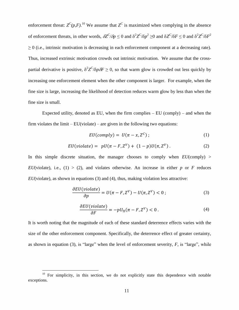
Expected utility, denoted as EU, when the firm complies – EU (comply) – and when the

firm violates the limit – EU(violate) – are given in the following two equations:

𝐸𝑈(𝑐𝑜𝑚𝑝𝑙𝑦) = 𝑈(𝜋 − 𝑥, 𝑍𝐶) ; (1)

𝐸𝑈(𝑣𝑖𝑜𝑙𝑎𝑡𝑒) = 𝑝𝑈(𝜋 − 𝐹, 𝑍𝑉) + (1 − 𝑝)𝑈(𝜋, 𝑍𝑉) . (2)

In this simple discrete situation, the manager chooses to comply when EU(comply) >

EU(violate), i.e., (1) > (2), and violates otherwise. An increase in either p or F reduces

EU(violate), as shown in equations (3) and (4), thus, making violation less attractive:

𝜕𝐸𝑈(𝑣𝑖𝑜𝑙𝑎𝑡𝑒)

𝜕𝑝= 𝑈(𝜋 − 𝐹, 𝑍𝑉) − 𝑈(𝜋, 𝑍𝑉) < 0 ; (3)

𝜕𝐸𝑈(𝑣𝑖𝑜𝑙𝑎𝑡𝑒)

𝜕𝐹= −𝑝𝑈Π(𝜋 − 𝐹, 𝑍𝑉) < 0 . (4)

It is worth noting that the magnitude of each of these standard deterrence effects varies with the

size of the other enforcement component. Specifically, the deterrence effect of greater certainty,

as shown in equation (3), is “large” when the level of enforcement severity, F, is “large”, while

10

For simplicity, in this section, we do not explicitly state this dependence with notable

exceptions.

12

the deterrence effect of greater severity, as shown in equation (4), is large when the level of

enforcement certainty, p, is large.

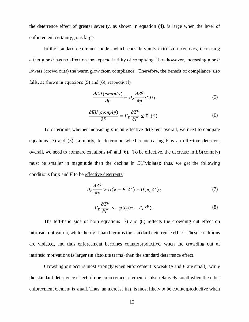
In the standard deterrence model, which considers only extrinsic incentives, increasing

either p or F has no effect on the expected utility of complying. Here however, increasing p or F

lowers (crowd outs) the warm glow from compliance. Therefore, the benefit of compliance also

falls, as shown in equations (5) and (6), respectively:

𝜕𝐸𝑈(𝑐𝑜𝑚𝑝𝑙𝑦)

𝜕𝑝= 𝑈𝑍

𝜕𝑍𝐶

𝜕𝑝≤ 0 ; (5)

𝜕𝐸𝑈(𝑐𝑜𝑚𝑝𝑙𝑦)

𝜕𝐹= 𝑈𝑍

𝜕𝑍𝐶

𝜕𝐹≤ 0 (6) . (6)

To determine whether increasing p is an effective deterrent overall, we need to compare

equations (3) and (5); similarly, to determine whether increasing F is an effective deterrent

overall, we need to compare equations (4) and (6). To be effective, the decrease in EU(comply)

must be smaller in magnitude than the decline in EU(violate); thus, we get the following

conditions for p and F to be effective deterrents:

𝑈𝑍

𝜕𝑍𝐶

𝜕𝑝> 𝑈(𝜋 − 𝐹, 𝑍𝑉) − 𝑈(𝜋, 𝑍𝑉) ; (7)

𝑈𝑍

𝜕𝑍𝐶

𝜕𝐹> −𝑝𝑈Π(𝜋 − 𝐹, 𝑍𝑉) . (8)

The left-hand side of both equations (7) and (8) reflects the crowding out effect on

intrinsic motivation, while the right-hand term is the standard deterrence effect. These conditions

are violated, and thus enforcement becomes counterproductive, when the crowding out of

intrinsic motivations is larger (in absolute terms) than the standard deterrence effect.

Crowding out occurs most strongly when enforcement is weak (p and F are small), while

the standard deterrence effect of one enforcement element is also relatively small when the other

enforcement element is small. Thus, an increase in p is most likely to be counterproductive when

13

F is small, and vice versa. When p or F are large, then extrinsic motivation dominates intrinsic

motivation with the standard deterrence story prevailing.

In order to address our main research question regarding the relative effectiveness of

certainty versus severity of punishment, we next derive the response elasticities with respect to

the two components of enforcement.11

First, consider the standard deterrence model, which

considers only extrinsic motivation. In this case, the relative effectiveness of the two components

depends on the risk preferences of the decision-maker (Becker, 1968). For risk- loving

managers, increasing the probability of detection, p, has a larger impact on deterrence than an

equivalent increase in the fine size, F, while increasing the fine size, F, has a larger impact on

deterrence than an equivalent increase in the probability of detection, p, for risk- averse

managers. Risk-neutral managers are indifferent between equivalent increases in p and F.

Second, consider our general model with intrinsic motivation. This consideration involves

comparing the effect of each enforcement component on the warm glow generated by

compliance, ZC. This comparison involves three possible cases: (1) increasing p is more

detrimental to warm glow than increasing F, (2) increasing F is more detrimental to warm glow

than increasing p, and (3) both increases are equally detrimental.

In order to assess the overall effectiveness of each enforcement component and to

compare the two effects, we must consider all nine possible combinations of the three risk

preference structures and the three rankings of warm glow effects. Table 1 summarizes the nine

cases, each case representing a separate hypothesis. Given risk-loving preferences, in the

absence of warm glow considerations or with equally detrimental effects, an increase in p is a

more effective deterrent than an increase in F. If an increase in F is more detrimental to warm

glow than an increase in p, then this comparison reinforces the standard result. If an increase in

11

Full details of these derivations and comparisons are available from the authors upon request.

In the interest of brevity, we include only an intuitive discussion here.

14

p is more detrimental to warm glow than an increase in F, the ranking reverses when the

crowding out of warm glow by increasing p is large enough to override the standard comparative

deterrence effect. This case is most likely when the crowding out effect from an increase in p is

large (p and F are small) and the difference in the standard deterrence effects of p and F is small

(preferences are weakly risk loving, p and F small).

Given risk-averse preferences, in the absence of warm glow effects or with equally

detrimental effects, an increase in F is a more effective deterrent than an increase in p. This

effect is reinforced when an increase in p causes more crowding out than an increase in F. The

direction switches only if an increase in F is sufficiently damaging to warm glow that the

countervailing effect overrides the standard comparative deterrence effect. This case is most

likely when the crowding out from an increase in F is large and the difference in the standard

deterrence effects is small (weak risk aversion, p and F small). Given risk-neutral preferences,

the relative crowding out effects determine the comparison of overall effects because the

standard prediction is equal efficacy.

Our theoretical model demonstrates that, once broader considerations are embedded in

the standard deterrence model, no clear prediction emerges regarding the relative efficacy of the

enforcement components. It therefore becomes an empirical question as to which cases arise in

practice. When enforcement is weak, as it often is in practice, intrinsic motivation is important.

When enforcement is strong, then intrinsic motivation is relatively small; consequently, the cases

shown in the middle column of Table 1 (i.e., increases in severity and certainty are equally

detrimental to warm glow) are the most relevant.

Beyond the results comparing the relative effectiveness of a higher likelihood of

punishment and a larger fine, our theoretical model generates two additional insights. First,

equations (3) and (4) reveal that the magnitudes of the effects associated with the enforcement

parameters (p and F) are not constant but instead vary with the strength of the other enforcement

15

parameter. Second, the nature of the likelihood variable (p) is clearly shown as the likelihood of

being detected and fined. In contrast, empirical models typically use inspection likelihood as the

proxy for this measure, which is inconsistent with the theoretical framework.

Finally, note that firm managers’ perceptions about the enforcement process might

generate a second type of effect that runs counter to standard deterrence. Unlike in the Becker

model, likelihood and severity are unknown variables about which firm managers must form

expectations based on their own experiences and that of related firms. If expectations are

unbiased on average, then an increase in the actual likelihood translates into an increase in the

perceived likelihood, thereby, enhancing deterrence. On the other hand, firm managers may hold

perceptions about the regulatory process that prompt the opposite outcome. For example, firm

managers may believe that the enforcer faces a fixed budget; if true, increased enforcement

against other firms may lead an individual firm manager to lower his/her perceived likelihood.12

Alternatively, experiencing enforcement may lead an individual firm manager to lower his/her

perception of enforcement likelihood in the future due to an effect like the gambler’s fallacy, “a

belief in negative autocorrelation of a non-autocorrelated random sequence” (Croson and

Sundali, 2005, p.195).13

These misperceptions of probability provide an additional pathway

through which increasing certainty could be counterproductive for deterrence. While not

formally modeled, these mechanisms intuitively increase the likelihood that the cases shown on

the right-hand column of Table 1 (i.e., increase in certainty is more detrimental to warm glow)

are the more relevant.

12

See Heyes and Kapur (2009) for a theoretical model where the enforcer is budget driven.

13

Inspections and enforcement are clearly not random processes; nevertheless, the point remains.

See also Tversky and Kahneman (1974).

4. Econometric Framework

To assess empirically the relative efficacy of enforcement likelihood and severity, we

construct an econometric framework that reflects the conceptual framework, while incorporating

additional control factors. In each period, the manager running the firm must make a compliance

decision. Hereafter we assume that each firm operates a single regulated facility. In order to study

both improvement toward compliance and improvement beyond compliance, we construct the

dependent variable as the ratio of actual discharges to permitted discharges, i.e., discharge ratio,

which captures the extent of compliance (Earnhart, 2004a,b,c; Earnhart, 2009; Earnhart and

Segerson, 2012). We formulate a set of primary explanatory variables measuring regulatory

enforcement and monitoring, collectively reflecting regulatory interventions, from which we capture

the certainty and severity of enforcement.

Each facility must form expectations about enforcement before selecting its extent of

compliance. Our empirical analysis assumes that each facility bases its expectations of future

enforcement on the experiences of other similar facilities along with its own recent experiences

(Shimshack and Ward, 2005; Earnhart, 2004a,b,c; Earnhart, 2009). General deterrence reflects the

ex ante general “threat” of future punishment based on the recent experiences of other facilities with

regulatory interventions (Sah, 1991; Cohen, 2000). Specific deterrence adjusts this general threat

based on the specific enforcement experiences of particular facilities in the recent past (Cohen, 2000;

Earnhart and Friesen, 2013). Facilities most likely need at least a few weeks, if not several months,

to respond to their own and others’ experiences with regulatory interventions. Thus, our analysis

lags the measures of inspections and enforcement actions (Earnhart, 2004a,b; Earnhart, 2009;

16

Shimshack and Ward, 2005).15

Most important for our comparison of enforcement certainty versus severity, we measure

sanction likelihood in three ways and sanction severity in two ways, generating three “models” in

the process. For Model 1, we follow the existing literature by letting inspections serve as our

measure of sanction likelihood while including the average sanction monetary value as our measure

of sanction severity (Shimshack and Ward, 2005). For Model 2, we let inspections measure sanction

likelihood while including the sanction conditional average amount, i.e., dollars per sanction

imposed, as our measure of sanction severity. This second measure of sanction severity is more

accurate because it excludes zero values when no sanction is imposed. As Model 3, we let sanction

count serve as our measure of sanction likelihood, while including sanction conditional average

amount as our measure of sanction severity, yet retaining inspections as a regressor. Using this

model, we more accurately interpret the effect of inspections as reflecting regulatory presence,

technical assistance, and regulatory burden (i.e., hassle of hosting the regulatory inspector, which

represent costs independent of sanctions). By controlling for the use of inspections, we more

effectively interpret the effect of sanction count as capturing a facility’s response to an agency’s

willingness to translate inspections into enforcement, i.e., certainty of punishment conditional on

inspections. Thus, we use a more theoretically relevant measure of likelihood since, as noted in

Section 3, likelihood refers to the likelihood of a sanction.

We argue that this third model represents a contribution to the literature for these reasons.

(1) Inspections are not necessarily prompted by non-compliance, which mutes the threat of

The theoretical framework captures equilibrium conditions in which contemporaneous measures15

of the enforcement threat influence current compliance conditions. The econometric framework capturesresponses to recent enforcement experiences. Contemporaneous enforcement measures should not influencecompliance decisions especially in the case of inspections conducted at and enforcement actions takenagainst other facilities.

17

inspections leading to sanctions since some inspections are not able to detect non-compliance. (2)

Inspections are not required to impose sanctions: self-reported data on non-compliance are sufficient

to prompt sanctions. (3) Inspections that identify/confirm non-compliance need not lead to sanctions

due to enforcement discretion on the part of regulatory agencies.16

With these approaches in mind, we construct the following particular deterrence factors.

When capturing general deterrence stemming from enforcement sanctions, the analysis examines the

aggregate count and monetary value of sanctions (in dollars) imposed against all other similar

facilities – major chemical facilities in the same state – over the preceding 12-month period. To

calculate the unconditional average sanction, our analysis divides each aggregate monetary value of

sanctions by the number of months other major chemical facilities were operating in each state over

the given 12-month period. This division controls for differences in the extent of operation of major

chemical facilities across states and over time. For this reason, we apply the same division to the

aggregate count. The resulting measures respectively represent the likelihood of a sanction imposed

on another similar facility per month of operation and the unconditional average sanction amount

imposed against other similar facilities per month of operation.17

To measure specific deterrence stemming from enforcement, we consider sanctions imposed

on an individual facility in the preceding 12-month period, consistent with previous empirical studies

(Earnhart, 2004a,b; Earnhart, 2009), which treat these lagged sanctions as an exogenous regressor.

We assess this treatment below. For comparability with the sanction-based general deterrence

Two previous studies on regulatory enforcement support our claim that use of enforcement actions16

to construct a measure of enforcement likelihood dominates the use of inspections to construct this measure;Gray and Scholz (1991, 1993) find that only OSHA inspections resulting in a penalty, not all types ofinspections, lower injury rates.

For clarity, if each facility operates all 12 months within the preceding 12-month window, then17

the resulting measures simply reflect the likelihood of the average facility being sanctioned and theunconditional average sanction size, respectively.

18

measures, our analysis divides each aggregate value of sanctions by the number of months the

specific individual facility was operating over the given 12-month period. The resulting measures

represent the likelihood of a sanction imposed on the specific facility per month of operation and the

unconditional average sanction amount imposed against the specific facility per month of operation.

We also assess the influence of inspections on compliance decisions. As with sanctions,

regulated facilities must gauge the threat of an inspection. To capture this threat, our analysis

employs a proxy based on the annual aggregate count of inspections against other similar facilities

– major chemical facilities in the same state – over the preceding 12-month period. Given the

discrete nature of monitoring, a simple count of inspections seems sufficient. Our analysis divides18

the aggregate count of inspections by the number of months other major chemical facilities were

operating in each state over the 12-month period.19

Regarding specific deterrence, we assess inspections conducted at the individual facility in

the preceding 12-month period, consistent with several previous empirical studies (Magat and

Viscusi, 1990; Helland, 1998a,b; Earnhart, 2004a,b; Earnhart, 2009), which treat these lagged

inspections as an exogenous regressor. Again we assess this treatment below. We divide the

number of inspections by the number of months a particular facility was active in the preceding 12-

month period. Thus, the constructed regressor measures inspections per month of activity.

In the case of inspections, the chosen 12-month period is warranted since federal regulations18

dictate that major polluters should be inspected once per year (EPA, 1990).

The sanction- and inspection-related general deterrence measures should not depend on the19

particular facility’s performance since the interventions are imposed against other facilities. Instead, these“other” interventions should depend on other facilities’ compliance. In addition, it is highly doubtful thatone facility’s performance directly depends on other facilities’ performance. [Of course, all facilities’performance may depend upon common factors, such as seasons (e.g., treatment may be more difficult incold weather)]. Instead of improbable connections across individual firms’ compliance levels, the generaldeterrence measures rely upon factors that are common to all similar facilities, e.g., location in a given state. These common factors capture exogenous elements of regulatory pressure: exogenous variation in regulatorypressure across states and time.

19

Regardless of the two measures used to capture the certainty and severity of enforcement, we

allow the two measures to influence each other, consistent with the theoretical framework

constructed in Section 4, by generating an interaction between the two factors for each dimension

of deterrence: general and specific. Thus, the deterrent effect of each enforcement component –

likelihood and severity – can depend on the size of the other enforcement component.

To identify the remaining independent variables, we draw upon the factors relating to the

costs of compliance and non-compliance, while offering a priori expectations on the factors’ effects.

The first set of control factors relate to the costs of non-compliance. We incorporate additional

regulatory factors (Helland, 1998a; Earnhart, 2004a,b; Nadeau, 1997). First, we capture variation

in regulatory pressure not reflected in the enforcement measures by including two regressors that

separately measure annual budgetary resources expended by state and local agencies (by state) and

EPA regional offices (by region). Each budgetary measure is adjusted by the number of

manufacturing facilities in each state and region, respectively, for the relevant year. As budgetary

resources increase, the discharge ratio should decline. We also include EPA regional indicators,

which should control for any meaningful regional variation in monitoring and enforcement not

reflected in the deterrence measures.

Second, we include facility-specific NPDES permit conditions as regressors, which capture

certain dimensions of regulatory stringency: (1) the permitted effluent limit (in pounds/day); (2) the

limit type [initial or interim versus final]; and (3) an indicator for any modification(s) to the NPDES

permit after issuance. As limits tighten, the discharge ratio should rise given increasing marginal

abatement costs. Facilities might perceive final limits as more legally meaningful; if true, final limits

should induce lower discharge ratios than initial or interim limits. Facilities might view permit

modifications as indications of a cooperative regulatory approach, which might induce facilities to

20

respond in kind with lower discharge ratios. We also include a set of individual EPA region

indicators and individual calendar year indicators, which contain no obvious a priori expectations.

In addition to regulatory pressure, we allow ownership structure to control for variation in

investor pressure. Facilities owned by publicly held firms are expected to discharge less because

publicly held firms face greater pressure from investors for good environmental performance.20

The second set of control factors relate to the costs of compliance, i.e., costs of abatement.

Specifically, facility and firm characteristics influence marginal abatement costs, which in turn affect

the chosen extent of compliance (Earnhart, 2004a; Bandyopadhyay and Horowitz, 2006; Gray and

Shadbegian, 2005). Flow design capacity represents one dimension of facility size. Regulated21

facilities may enjoy economies of scale or confront diseconomies of scale regarding pollution

control. The ratio of actual wastewater flow to flow design capacity may proxy for treatment

capacity utilization. As utilization rises, marginal abatement costs most likely increase. The

volatility of wastewater discharges, as measured by the standard deviation of TSS relative discharges

over a current calendar year, captures the pattern of discharges. As discharge volatility rises,

facilities may choose to decrease their “expected” discharge ratio in a probabilistic sense in order

to reduce the likelihood of exceeding their limits ex post. Industrial sub-sector indicators, which are

As a second form of external pressure, we attempt to control for local community pressure20

indirectly using certain community characteristics [Hamilton, 1993; Earnhart, 2004c; Bandyopadhyay andHorowitz, 2006]: (1) wealth, as measured by per capita income; (2) local labor market conditions, asmeasured by the unemployment rate; (3) urban versus rural context, as measured by population density; (4)ethnic composition, as measured by the proportion of non-white residents; (5) reliance on economic activity,as measured by the proportion of private earnings generated by chemical manufacturing; (6) politicalengagement, as measured by the voter turnout rate. Collectively, these factors do not prove relevant in ourestimation results. (Based on the dominant fixed effects estimates, the relevant partial F-test statistics are1.07, 1.08, and 1.14, respectively, for Models 1, 2, and 3, with p-values of 0.380, 0.375, and 0.338.) Thus,we do not report estimation results that stem from regressor sets including the local community factors. Nevertheless, we provide details on the relevant data sources in Appendix A.

Since the EPA does not systematically provide data on flow design capacity, this study uses a21

proxy: the average flow of wastewater (millions of gallons per day) over the preceding 12-month period.

21

fully listed on Table 2.b, help to control for variation in facilities’ abilities to adjust their production

processes based on the type of product being manufactured. Thus, the type of production process,

as proxied by sub-sectoral classifications, influences marginal abatement costs but without a priori

expectations regarding the effect of production process on the chosen discharge ratio. Seasonal

indicators control for variation prompted by weather conditions, which may influence facilities’

treatment (or production) processes without strong a priori expectations.

Abatement costs also depend on ownership structure, which we measure by contrasting

publicly held structures from all other ownership structure. Facilities owned by publicly held firms

are expected to discharge less (i.e., lower discharge ratio) because publicly held firms enjoy greater

access to external financing. As noted above, we also use ownership structure to control for

variation in investor pressure.

5. Data

For the construction of the dependent and independent variables, we gather data from various

sources: EPA Permit Compliance System database (discharge limits, actual discharges, permit

features, inspections, fines); EPA Docket database (fines, injunctions, SEPs); and Compustat

database (firm-level ownership structure).22

The broadest sample includes all of the monthly observations for the 508 facilities that were

active at some point over the sample period: January, 1995, to June, 2001. To remain in the sample,

a given facility must discharge TSS at least once during the seven-year sample period, which

identifies 461 facilities. Moreover, a given facility must face an effluent limit for TSS in the

particular month of discharge. This restriction eliminates 3,152 observations, dropping the sample

size from 32,378 to 29,226. Since the regressor list includes various measures based on a preceding

Appendix A provides details on the data sources and the regression sample selection.22

22

12-month period (e.g., cumulative count of sanctions), the regression sample period starts on

January, 1996. Consequently, the relevant sample size drops to 23,193, consisting of 406 facilities.

Table 2 provides statistical summaries of the formulated dependent variable and regressors.

Table 2.a summarizes the environmental performance measures. The mean discharge ratio of 0.315

implies that facilities on average generate TSS discharges that are 68.5 % below their monthly limits.

This average indicates a need to analyze the extent of compliance rather than the status of

compliance. The maximum discharge ratio of 9.080 implies that facilities allow their TSS

discharges to surge as high as 808.0 % above the permitted limits. This maximum indicates a need

to analyze the degree of non-compliance rather than the extent of non-compliance. Table 2.b23

summarizes the regressors.

6. Econometric Analysis and Estimation Results

6.1. Econometric Issues

In order to estimate the relationship between the discharge ratio and the regressors, we must

address several econometric issues. First, we employ a mixed log-log specification. We log the

dependent variable because discharge ratios are distributed lognormal. Logging the enforcement-

and inspection-related regressors simplifies the process of comparing the effects of certainty of

enforcement versus severity of enforcement because the estimated coefficients reflect elasticities.

Based on our study and previous studies, regulated facilities regularly over-comply with their23

effluent limits (e.g., Earnhart, 2009; Earnhart and Segerson, 2012; Bandyopadhyay and Horowitz, 2006). The economics literature identifies various factors that may prompt over-compliance including pressureexerted by other external parties, such as local communities (Henriques and Sadorsky, 1996; Dasgupta et al.,2000), investors (Downing and Kimball, 1982), and customers (Arora and Cason, 1996). Stochasticdischarge patterns may also play a role (Bandyopadhyay and Horowitz, 2006). Even though our theoreticalframework treats discharges as deterministic, they are most likely stochastic to some extent. In this case,enforcement may still influence facilities’ environmental management decisions even when dischargesgenerally fall below effluent limits. Put differently, over-compliance in general may represent an ex antedecision to lower the likelihood of being non-compliant ex post. Our empirical analysis incorporatesregressors that capture these relevant factors for inducing over-compliance. This understanding provides alink to our theoretical model in which the decision to comply is binary and deterministic.

23

We do not log the non-deterrence regressors.24

We consider various regressor sets. As noted above, we estimate three models that differ

based on the deterrence factors. We consider four model sets that differ based on the non-deterrence

factors, i.e., control factors. Model Set A excludes all of the non-deterrence factors, representing the

most parsimonious model set. Model Set B includes the most basic control factors: year indicators,

seasonal indicators, EPA regional indicators, and sub-sector indicators. Model Set C additionally

includes the non-deterrence regulatory factors: permit conditions and budgetary resources. Finally,

Model Set D further adds facility and firm characteristics.

We address the panel structure of our data by employing three standard panel estimators:

pooled OLS, random effects, and fixed effects. Regardless of the estimator, we cluster the standard

errors on the regulated facility, which helps to address serial correlation. Our econometric analysis

uses the appropriate tests to discern the “best” panel estimator. We report the test results in the last

two rows of Table 3. Based on F-test for Fixed Effects statistics, the fixed effects estimator

dominates the pooled OLS estimator in all estimated cases. Based on Hausman Test for Random

Effects statistics, the fixed effects estimator dominates the random effects estimator since the latter

estimator appears inconsistent in all estimated cases. Given these test results, our study focuses

exclusively on the fixed effects estimates.25

Zero discharges (which are present in 0.68 % of sample) are set equal to the log of the smallest24

positive ratio in the regression sample. This approach assumes that every facility pollutes at least a little bitevery month; therefore, the reported value of zero is merely an approximation of some small positivedischarge level. Similarly, to address the presence of zero values in our enforcement measures, we use a verysmall value, relative to the sample distribution, to serve as a reasonable approximation of some minimalthreat of enforcement or inspection, i.e., a threat is always present even no government interventions wererecently conducted.

Thus, identification in our estimations stem exclusively from intra-facility variation. By25

construction, all time-invariant factors, including the EPA regional indicators and industrial sub-sectorindicators, are subsumed into the facility-specific fixed effects.

24

When considering the various model sets, estimation results show that Model Set D proves

the best set of regressors, regardless of the model used to capture the certainty and severity of

enforcement and the type of panel estimator.26

Lastly, we address the potential endogeneity of the specific deterrence regressors even though

they represent lagged measures. We address this potential concern by employing an instrumental

variable (IV) estimator, namely, fixed effects two-stage least squares. Our analysis generates test

statistics that reveal our chosen instruments appear relevant and not invalid. As important, the IV

estimation generates Durbin-Wu-Hausman Exogeneity Test statistics that fail to reject the null

hypothesis of exogeneity for Models 1, 2, and 3, which indicate that the specific deterrence

regressors do not appear endogenous. IV estimation when the regressors are uncorrelated with the

error process involves an important cost – “the asymptotic variance of the IV estimator is always

larger, and sometimes much larger, than the asymptotic variance of the OLS estimator” (Wooldridge,

2002, p. 490). Therefore, we proceed with the standard fixed effects estimator when estimating the

functional relationship between the discharge ratio and various regressor sets. Appendix B provides

full details on our assessment of the potentially endogenous specific deterrence regressors.27

Based on partial F-test statistics, the additional regressors in Model Set D relative to Model Sets26

A, B, and C prove jointly significant. We report only the partial F-test statistics derived from the dominantfixed effects estimates. For Model 1, the F-test statistics are 4.03, 1.35, and 2.98, respectively, for ModelSets A, B, and C, with p-values of 0.001, 0.209, and 0.019. For Model 2, the F-test statistics are 4.03, 1.35,and 2.98, respectively, for Model Sets A, B, and C, with p-values of 0.001, 0.208, and 0.019. For Model 3,the F-test statistics are 3.95, 1.38, and 3.03, respectively, for Model Sets A, B, and C, with p-values of 0.001,0.193, and 0.018. (In the case of Model Set D versus Model Set B, we ignore the lack of joint significancesince it is driven solely by the limited traction offered by the permit condition regressors and because ModelSet D still dominates Model Set C, which subsumes Model Set B.) Thus, we focus on Model Set D. Fortunately, our conclusions prove robust to the choice of model set with only minor exceptions.

Our assessment of the exogeneity regarding specific deterrence factors represents a contribution27

to the literature, albeit a minor one, since no previous study addresses the potential endogeneity to anymeaningful extent. Appendix B describes previous studies’ treatment of specific deterrence factors.

25

6.2. Estimation Results

Our empirical analysis considers three sets of deterrence measures – Models 1, 2, and 3 –

that differ based on the manner for capturing the certainty and severity of enforcement. Table 3

reports the fixed effects estimates for the control factors for Models 1 through 3, one column for each

model. Tables 4, 5, and 6 report the deterrence factor estimates for Models 1, 2, and 3, respectively,

with the main and interactive coefficients shown in Tables 4.1, 5.1, and 6.1. Due to the presence of

the interaction term between the certainty of enforcement and severity of enforcement, the main

coefficients are only interpretable when the paired enforcement component equals zero, which is

severely limiting. Consequently, we explore the marginal effects of the deterrence factors by

evaluating each enforcement component at more meaningful values of the other enforcement

component, as shown in Tables 4.2, 5.2, and 6.2, respectively, for Models 1, 2, and 3. In order to

span the full range of a marginal effect, Tables 4.2, 5.2, and 6.2 evaluate each marginal effect at the

other enforcement component’s minimum and maximum values. Lastly, Tables 4, 5, and 6 test

whether the marginal effect of certainty and the marginal effect of severity are equal in magnitude.

In order to compare two marginal effects, we must identify a combination of values: one for each

enforcement component. To span the range of both marginal effects, we consider these four

combinations:

I. Certainty Value = minimum, Severity value = minimum;

II. Certainty Value = maximum, Severity value = maximum;

III. Certainty Value = maximum, Severity value = minimum; and

IV. Certainty Value = minimum, Severity value = maximum.

Tables 4.2, 5.2., and 6.2 assess combinations I and II; Tables 4.3, 5.3, and 6.3 assess combinations

III and IV.

26

6.2.1. Deterrence Factors

6.2.1.1. Individual Effects

We first interpret the deterrence-related coefficients starting with the Model 1 estimates

shown in Table 4. Neither of the interactive terms is statistically significant, the marginal effects of

certainty and severity never prove statistically significant, and the two marginal effects do not

statistically differ from one another. Overall, the Model 1 estimates reveal that certainty and severity

of enforcement are equally ineffective at inducing better compliance with wastewater discharge

limits. The Model 2 estimates, shown in Table 5, lead us to draw conclusions identical to those

drawn from the Model 1 estimates.

In stark contrast, the Model 3 estimates, shown in Table 6, prove very interesting and confirm

our expectation that Model 3 is the best model for discerning and comparing the effects of certainty

versus severity of enforcement. First, the interactive terms reveal that synergies exist between the

certainty and severity of enforcement. Thus, inclusion of these interactive terms is warranted given

the strong statistical significance. The negative interactive terms reveal that the two enforcement

components are complements: as one enforcement component increases, the marginal effect of the

other component becomes more negative (i.e., more effective at lowering the discharge ratio).

Consistent with this classification, as shown in Table 6.2, the marginal effect of each

enforcement component is positive when the other component is set at its minimum value, yet the

marginal effect is negative when the other component is set at its maximum. Positive marginal

effects demonstrate that deterrence is counter-productive. Two of these counter-productive effects

prove statistically significant. An increase in specific deterrence enforcement severity leads to

significantly higher discharge ratios, i.e., less compliance, as does an increase in general deterrence

enforcement certainty. Negative marginal effects demonstrate that deterrence is effective at

27

improving compliance. All four of the effective marginal effects prove statistically significant.

Thus, regardless of the type of deterrence – specific or general – and the component of enforcement

– certainty or severity, greater enforcement leads to lower discharge ratios, i.e., better compliance.

While one might hope that greater enforcement would never prove counter-productive, if not

always effective, our theoretical analysis in Section 3 reveals this possibility and our empirical

results demonstrate that under particular conditions, greater enforcement appears to generate

countervailing effects. In particular, we conclude that, based on an individual facility’s own

experience with enforcement, an increase in the conditional average sanction magnitude, reflecting

greater enforcement severity, appears to undermine intrinsic motivation when the likelihood of a

sanction is very small. Perhaps regulated facilities are annoyed by an enforcement regime that does

not seem to generate a level playing field. In contrast, we conclude that, based on other facilities’

experiences with enforcement, an increase in the likelihood of a sanction, based on the count of

sanctions per month and reflecting greater enforcement certainty, appears to distort perceptions of

the likelihood of enforcement when the severity of a sanction is very small. Perhaps under these

conditions regulated facilities believe that the “storm has passed” once other facilities are sanctioned.

Alternatively, the imposition of small penalties on others may generate ill will toward the regulator.

In order to explore more fully the marginal effects relating to enforcement components, we

construct Figure 1 based on the fixed effects estimates for Model 3. For each enforcement

component, it displays the marginal effects, along with the associated 90 % confidence intervals,

across the full range of values for the other enforcement component. The upper panels of Figure 1

display the specific deterrence marginal effects, while the lower panels of Figure 1 display the

general deterrence marginal effects.

As shown in the upper left panel of Figure 1, the marginal effect of specific deterrence-

28

related enforcement certainty is significantly negative, i.e., increased certainty is effective at inducing

better compliance, over a majority of the relevant range and never significantly positive, i.e., counter-

productive. In contrast, the marginal effect of specific deterrence-related enforcement severity is

significantly negative for only a portion of the relevant range and significantly positive over a

comparable portion of the relevant range, as shown in the upper right panel of Figure 1. The

marginal effect of general deterrence-related enforcement certainty is significantly positive,

statistically zero, and significantly negative across roughly equal portions of the relevant range, as

shown in the lower left panel of Figure 1. Thus, increases in the certainty of a sanction based on

other similar facilities’ experiences are counter-productive, ineffective, or effective at inducing better

compliance across the relevant range. In strong contrast, the marginal effect of general deterrence-

related enforcement severity is significantly negative for most of the relevant range and never

significantly positive. Therefore, the lower right panel of Figure 1 reveals that increases in the

severity of a sanction based on other similar facilities’ experiences are mostly effective at inducing

better compliance across the relevant range.

As one more means of exploring the individual marginal effects of certainty and severity, we

separately calculate the certainty effect and severity effect for each observation in the sample and

then assess whether the calculated effect significantly differs from zero. Table 7.a tabulates the

results. First consider specific deterrence, as shown in Table 7.a.i. The certainty effect is

significantly productive for only 1 % of the observations and statistically zero for the remaining

observations, thus, the effect is never significantly counter-productive. In contrast, the severity effect

is significantly counter-productive for 98.6 % of the observations and significantly productive for

only 0.4 % of the observations, while being statistically zero for the remaining 1 % of the

observations. Overall, specific deterrence is rarely productive. Next consider general deterrence,

29

as shown in Table 7.a.ii. The certainty effect is significantly counter-productive for 70 % of the

observations, yet significantly productive for 10 % of the observations, and statistically zero for 20

% of the observations. In contrast, the severity effect is significantly productive for 31 % of the

observations and never significantly counter-productive, yet statistically zero for 69 % of the

observations. Overall, these results demonstrate that counter-productive enforcement is not just a

theoretical possibility but also a reality in the examined enforcement regime.

6.2.1.2. Comparison of Marginal Effects

Based on the Model 3 results, we compare the marginal effects of certainty and severity,

which represents our study’s primary objective. Throughout our comparison, we conclude that one

marginal effect “dominates” the other marginal effect whenever the former proves the more effective

deterrent, i.e., the marginal effect is more negative or at least less positive. Tables 6.2 and 6.3 assess

the comparison of the two marginal effects when each enforcement component is set at either its

minimum or maximum. Consider first specific deterrence. When both certainty and severity are set

at their minima, both individual effects are positive, with the severity effect significantly counter-

productive, yet the two effects are statistically equal, i.e., equally counter-productive. However,

when both certainty and severity are set at their maxima, both individual effects prove significantly

negative, i.e., effective at reducing discharges, and the certainty effect dominates the severity effect.

When certainty is shifted to its minimum, the severity effect becomes significantly counter-

productive again. Not surprising, the certainty effect continues to dominate the severity effect.

Thus, if enforcement severity lies at an extremely high level, an increase in certainty proves more

effective than an increase in severity regardless of the certainty value. In contrast, if certainty is set

at its maximum and severity is set at its minimum, then the certainty effect becomes (insignificantly)

counter-productive, while the severity effect becomes significantly productive. In this case, the

30

severity effect dominates the certainty effect, i.e., an increase in severity proves more effective than

an increase in certainty for reducing discharges.

Consider next general deterrence. When both certainty and severity are set at their minima,

both individual effects are positive, with the certainty effect significant and the severity effect

marginally significant [p=0.119], yet the severity effect dominates the certainty effect since the

former is less counter-productive. However, when both certainty and severity are set at their

maxima, both individual effects are significantly productive and the certainty effect dominates the

severity effect. As with specific deterrence, when certainty is shifted to its minimum, the severity

effect becomes marginally significantly counter-productive again and the certainty effect continues

to dominate the severity effect. Thus, as with specific deterrence, if enforcement severity lies at an

extremely high level, an increase in certainty proves more effective than an increase in severity

regardless of the certainty value. In contrast, if certainty is set at its maximum and severity is set at

its minimum, then the certainty effect becomes significantly counter-productive, while the severity

effect becomes significantly productive, as with specific deterrence. Moreover, the severity effect

dominates the certainty effect.

In sum, the specific and general deterrence comparisons support identical conclusions

excepting the combination where each enforcement component is set at its minimum.

To explore further the comparison of the certainty and severity marginal effects, we compare

the certainty effect and severity effects calculated for each observation in the sample and then assess

whether the calculated certainty and severity effects are significantly different. Table 7.b tabulates

the results. First consider specific deterrence, as shown in Table 7.b.i. Interestingly, both marginal

effects are counter-productive for nearly 99 % of the observations (22,877 cases). In all of these

cases, the certainty effect dominates since its magnitude is less counter-productive [Region 2] yet

the difference between the two effects proves insignificant. In contrast, both marginal effects are

31

productive for only 1 % of the observations (282 cases). In all of these cases, the certainty effect

dominates the severity effect [Region 4], of which 82 % prove statistically significant. In the

remaining 41 cases (0.2% of observations), the severity effect dominates the certainty effect since

the former is productive, while the latter is counter-productive [Region 6], which never proves

statistically significant. No cases lie in Regions 1, 3, and 5.

Next consider general deterrence, as shown in Table 7.b.ii. As with specific deterrence, both

marginal effects are counter-productive for nearly 70 % of the observations (15,965 cases). In all

of these cases, the severity effect dominates since its magnitude is less counter-productive [Region

1] and the difference between the two effects proves significant. In contrast, both marginal effects

are productive for 26 % of the observations (6,039 cases). In most of these cases (4132 cases), the

certainty effect dominates the severity effect [Region 4], of which 43 % prove statistically

significant. In the remaining 1,907 cases, the severity effect dominates the certainty effect [Region

5], however, none of these cases prove statistically significant. For 5 % of observations, the severity

effect dominates the certainty effect since the former is productive, while the latter is counter-

productive [Region 6], which proves statistically significant in 81 % of the cases. For only three

observations the opposite holds: the certainty effect dominates the severity effect since the former

is productive, while the latter is counter-productive [Region 3]; all three cases the difference proves

statistically significant.

In sum, this assessment reveals that, based on specific deterrence, the certainty and severity

effects do not significantly differ in nearly all of the cases. Based on general deterrence, the severity

effect significantly dominates the certainty effect in many more cases than the reverse. Yet when

both effects are productive, the certainty effect significantly dominates the severity effect in more

cases than the reverse.

As a final means of comparing the marginal effects of certainty and severity, Figure 2

32

graphically displays the comparison of the two marginal effects across the full range of values for

the case of general deterrence. We do not provide an equivalent graph for specific deterrence

because, as shown in Table 7.b.i, almost all of the observations fall within one region, making a

graphical representation less informative. In Figure 2, the horizontal axis captures the level of the

certainty component, while the vertical axis captures the level of the severity component. Three lines

divide each graph into distinctive regions. The (vertical) line of zero elasticity with respect to

severity divides the graph into two regions: to the left of this line, the severity effect is counter-

productive; to the right of this line, the severity effect is productive. Similarly, the (horizontal) line

of zero elasticity with respect to certainty divides the graph into two regions: below this line, the

certainty effect is counter-productive; above this line, the certainty effect is productive. The

(positively sloped) line of equal elasticities divides the graph into two regions: left/above this line,

the certainty effect dominates the severity effect; right/below this line, the severity effect dominates

the certainty effect. Drawing upon all three lines, the graph divides into six distinctive regions based

on the productive/counter-productive aspect of each marginal effect and the comparison of the two

effects, as shown in Table 7.b. None of the described lines consider statistical significance; they rely

exclusively upon the magnitudes of the marginal effects; statistical significance is assessed in Table

7.b. Finally, Figure 2 overlays data on the sample distribution of each pairing of certainty level and

severity level, with each pairing shown as a blue diamond. By overlaying these data, we are able to

assess whether any given region proves relevant in the sample. Nevertheless, the graphs merely

display the distribution of the sample data; they do not show the frequency of observations within

each region. (The online appendix interprets the differences across the six regions shown in Figure

2 and classified in Table 7.b.)

Figure 2 shows the general deterrence-related regions and data pairings. With the exception

of zero severity values, the marginal effect of severity is never counter-productive. In contrast, the

33

marginal effect of certainty is counter-productive for several cases within the sample. In such cases,

the severity effect dominates the certainty effect. In all other cases, both marginal effects prove

productive. In several cases, the severity effect dominates, while in many other cases, the certainty

effect dominates. (Please note that Figure 2 curtails the vertical and horizontal range of the graph

in order to display the lines and data pairings effectively; in the process, a very few data pairings are

not displayed.) This graphical analysis helps to display the conclusions supported by Table 7.b and

to generalize the conclusions supported by Tables 6.2 and 6.3.

6.2.2. Control Factors

Lastly, we interpret the coefficients relating to the control factors, which are shown in Table

3. First, discharge ratios vary over the sample period from year to year. Second, discharge ratios

vary over the calendar year from season to season. Third, regulated facilities appear to confront

diseconomies of scale since discharge ratios rise as facilities get bigger. Fourth, facilities facing

greater volatility in their discharge patterns appear to comply less with their effluent limits. This

result runs counter to our a priori expectation. Future research should explore this point more

closely. All of these conclusions are fully robust across the three models.

7. Conclusions

Our study explores the relative efficacy of punishment certainty versus severity in prompting

better compliance with wastewater discharge limits. Clearly, a better understanding of this point is

important for policy considerations since enforcement agencies should place greater emphasis on the

more effective lever – certainty of punishment or severity of punishment. To improve this

understanding, our study examines the wastewater discharged by U.S. chemical manufacturing

facilities permitted within the Clean Water Act’s National Pollutant Discharge Elimination System

(NPDES) between 1995 and 2001 and effects of enforcement on facilities’ extent of compliance.

Our empirical results reveal that both specific and general deterrence can be significant

34

deterrents. However, the magnitude of the effects varies according to the perceived enforcement

threat. For low values of enforcement, increased certainty and severity are both counter-productive,

i.e., lead to greater pollution, with the effect of certainty larger in magnitude. These counter-

productive effects are consistent with our theoretical framework. Thus, counter-productive effects

are not only theoretical possibilities but also empirical realities within the examined enforcement

regime. Our results suggest that enforcement agencies should be cautious when increasing the

frequency of enforcement actions with low severity as the general deterrent effects of such actions

are likely to be counter-productive. On the other hand, increasing severity can be an effective

general deterrent but might prove counter-productive if such large punishments are infrequently

imposed. In contrast, when enforcement is high, both instruments are effective in deterring

pollution, although certainty is more effective. For intermediate values the results are more mixed.

As important, our results demonstrate the importance of including an interaction term between the

two components of deterrence: (1) certainty of punishment and (2) severity of punishment. This

interaction term reveals that certainty and severity are complements for both specific and general

deterrence.

These empirical results possess highly meaningful policy implications. Environmental

protection agencies should not rely upon a single component of enforcement – certainty or severity.

Otherwise, use of the stronger component proves counter-productive at inducing better compliance.

Instead, environmental protection agencies should employ both levers meaningfully so that both

tools prove effective. Nevertheless, the agencies should emphasize use of the certainty of

enforcement over the severity of enforcement when both levers are meaningfully employed. Future

research should explore whether or not these effects generalize to other environmental protection and

regulatory settings.

35

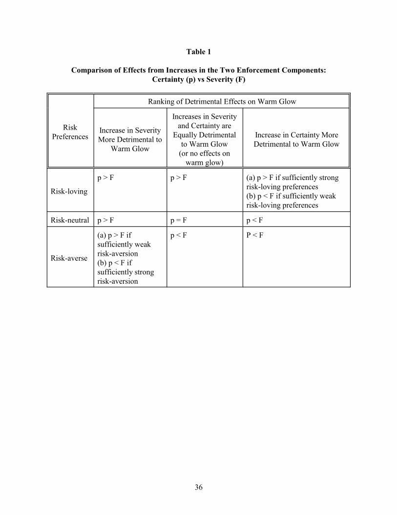
Table 1

Comparison of Effects from Increases in the Two Enforcement Components:Certainty (p) vs Severity (F)

RiskPreferences

Ranking of Detrimental Effects on Warm Glow

Increase in SeverityMore Detrimental to

Warm Glow

Increases in Severityand Certainty are

Equally Detrimentalto Warm Glow

(or no effects onwarm glow)

Increase in Certainty MoreDetrimental to Warm Glow

Risk-loving

p > F p > F (a) p > F if sufficiently strongrisk-loving preferences(b) p < F if sufficiently weakrisk-loving preferences

Risk-neutral p > F p = F p < F

Risk-averse

(a) p > F ifsufficiently weakrisk-aversion(b) p < F ifsufficiently strongrisk-aversion

p < F P < F

36

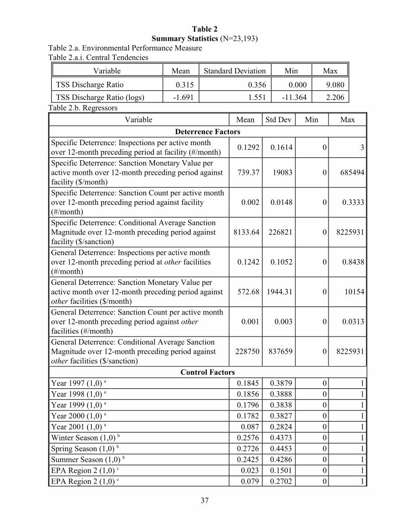
Table 2Summary Statistics (N=23,193)

Table 2.a. Environmental Performance MeasureTable 2.a.i. Central Tendencies

Variable Mean Standard Deviation Min Max

TSS Discharge Ratio 0.315 0.356 0.000 9.080

TSS Discharge Ratio (logs) -1.691 1.551 -11.364 2.206

Table 2.b. Regressors

Variable Mean Std Dev Min Max

Deterrence Factors

Specific Deterrence: Inspections per active monthover 12-month preceding period at facility (#/month)

0.1292 0.1614 0 3

Specific Deterrence: Sanction Monetary Value peractive month over 12-month preceding period againstfacility ($/month)

739.37 19083 0 685494

Specific Deterrence: Sanction Count per active monthover 12-month preceding period against facility(#/month)

0.002 0.0148 0 0.3333

Specific Deterrence: Conditional Average SanctionMagnitude over 12-month preceding period againstfacility ($/sanction)

8133.64 226821 0 8225931

General Deterrence: Inspections per active monthover 12-month preceding period at other facilities(#/month)

0.1242 0.1052 0 0.8438

General Deterrence: Sanction Monetary Value peractive month over 12-month preceding period againstother facilities ($/month)

572.68 1944.31 0 10154

General Deterrence: Sanction Count per active monthover 12-month preceding period against otherfacilities (#/month)

0.001 0.003 0 0.0313

General Deterrence: Conditional Average SanctionMagnitude over 12-month preceding period againstother facilities ($/sanction)

228750 837659 0 8225931

Control Factors

Year 1997 (1,0) 0.1845 0.3879 0 1a

Year 1998 (1,0) 0.1856 0.3888 0 1a

Year 1999 (1,0) 0.1796 0.3838 0 1a

Year 2000 (1,0) 0.1782 0.3827 0 1a

Year 2001 (1,0) 0.087 0.2824 0 1a

Winter Season (1,0) 0.2576 0.4373 0 1b

Spring Season (1,0) 0.2726 0.4453 0 1b

Summer Season (1,0) 0.2425 0.4286 0 1b

EPA Region 2 (1,0) 0.023 0.1501 0 1c

EPA Region 2 (1,0) 0.079 0.2702 0 1c

37

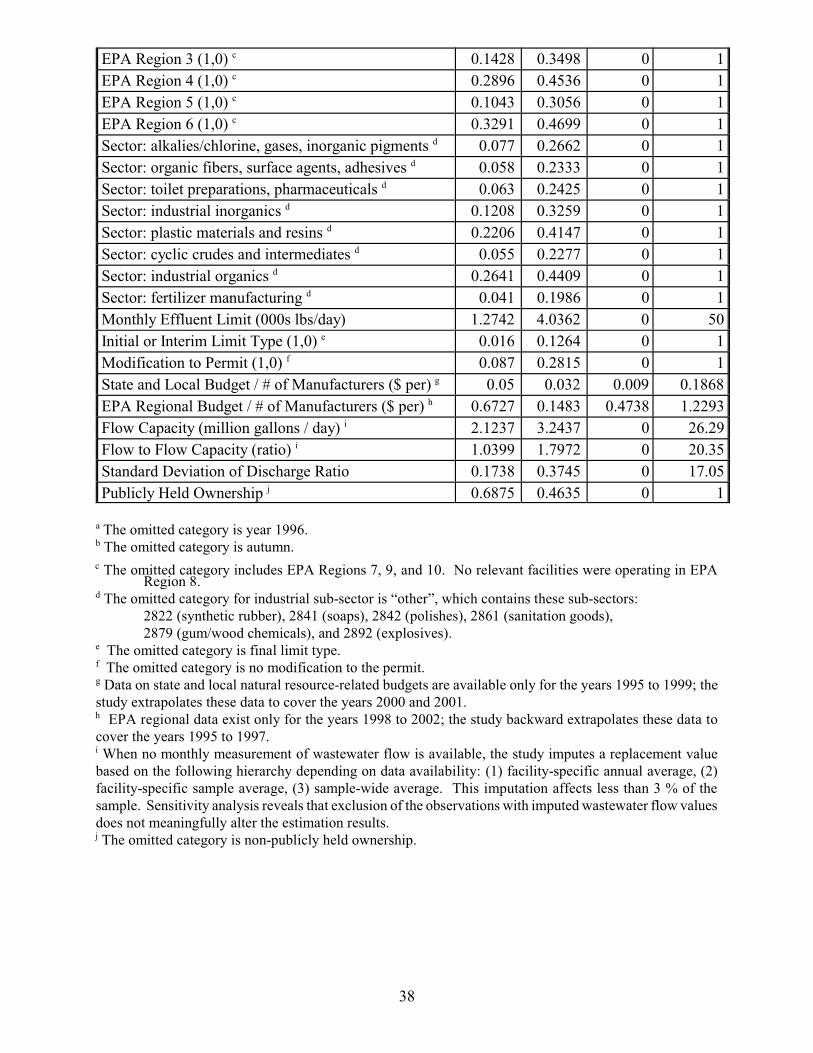
EPA Region 3 (1,0) 0.1428 0.3498 0 1c

EPA Region 4 (1,0) 0.2896 0.4536 0 1c

EPA Region 5 (1,0) 0.1043 0.3056 0 1c

EPA Region 6 (1,0) 0.3291 0.4699 0 1c

Sector: alkalies/chlorine, gases, inorganic pigments 0.077 0.2662 0 1d

Sector: organic fibers, surface agents, adhesives 0.058 0.2333 0 1d

Sector: toilet preparations, pharmaceuticals 0.063 0.2425 0 1d

Sector: industrial inorganics 0.1208 0.3259 0 1d

Sector: plastic materials and resins 0.2206 0.4147 0 1d

Sector: cyclic crudes and intermediates 0.055 0.2277 0 1d

Sector: industrial organics 0.2641 0.4409 0 1d

Sector: fertilizer manufacturing 0.041 0.1986 0 1d

Monthly Effluent Limit (000s lbs/day) 1.2742 4.0362 0 50

Initial or Interim Limit Type (1,0) 0.016 0.1264 0 1e

Modification to Permit (1,0) 0.087 0.2815 0 1f

State and Local Budget / # of Manufacturers ($ per) 0.05 0.032 0.009 0.1868g

EPA Regional Budget / # of Manufacturers ($ per) 0.6727 0.1483 0.4738 1.2293h

Flow Capacity (million gallons / day) 2.1237 3.2437 0 26.29i

Flow to Flow Capacity (ratio) 1.0399 1.7972 0 20.35i

Standard Deviation of Discharge Ratio 0.1738 0.3745 0 17.05

Publicly Held Ownership 0.6875 0.4635 0 1j

The omitted category is year 1996.a

The omitted category is autumn.b

The omitted category includes EPA Regions 7, 9, and 10. No relevant facilities were operating in EPAc

Region 8. The omitted category for industrial sub-sector is “other”, which contains these sub-sectors:d

2822 (synthetic rubber), 2841 (soaps), 2842 (polishes), 2861 (sanitation goods),2879 (gum/wood chemicals), and 2892 (explosives).

The omitted category is final limit type.e

The omitted category is no modification to the permit.f

Data on state and local natural resource-related budgets are available only for the years 1995 to 1999; theg

study extrapolates these data to cover the years 2000 and 2001. EPA regional data exist only for the years 1998 to 2002; the study backward extrapolates these data toh

cover the years 1995 to 1997. When no monthly measurement of wastewater flow is available, the study imputes a replacement valuei

based on the following hierarchy depending on data availability: (1) facility-specific annual average, (2)facility-specific sample average, (3) sample-wide average. This imputation affects less than 3 % of thesample. Sensitivity analysis reveals that exclusion of the observations with imputed wastewater flow valuesdoes not meaningfully alter the estimation results. The omitted category is non-publicly held ownership.j

38

Table 3Fixed Effects Estimation of TSS Discharge Ratio

Control Factor Coefficients: Magnitudes and p-valuesModels 1, 2, and 3 (N = 23,193)

RegressorModel 1 Model 2 Model 3

Magnitude p-value Magnitude p-value Magnitude p-value

Year 1997 -0.0755 0.030 -0.0737 0.035 -0.0773 0.028Year 1998 -0.0855 0.147 -0.0863 0.143 -0.0845 0.154Year 1999 -0.1912 0.052 -0.1895 0.054 -0.2006 0.041Year 2000 -0.1248 0.118 -0.1227 0.125 -0.1241 0.118Year 2001 -0.2157 0.073 -0.2145 0.075 -0.2279 0.058

Winter Season 0.1441 0.000 0.1442 0.000 0.1395 0.000a

Spring Season 0.1232 0.000 0.1235 0.000 0.1192 0.000a

Summer Season 0.0494 0.007 0.0501 0.006 0.0476 0.010a

Initial/Interim Limit Type -0.0172 0.875 -0.0169 0.878 -0.0176 0.872b

Modification to Permit -0.0565 0.682 -0.0568 0.681 -0.0585 0.674c

Monthly Effluent Limit 0.0187 0.738 0.0187 0.739 0.0187 0.739

State and Local Budget / # ofManufacturers

-1.2044 0.633 -1.2031 0.636 -1.7300 0.493

EPA Regional Budget / # ofManufacturers

0.2228 0.738 0.1908 0.774 0.4634 0.469

Flow Capacity 0.0993 0.065 0.0993 0.065 0.0996 0.064

Flow to Flow Capacity 6.6785 0.463 6.6877 0.462 6.5989 0.468

Std Dev of Discharge Ratio 0.2321 0.011 0.2322 0.011 0.2300 0.011Publicly Held Ownership 0.0704 0.394 0.0704 0.393 0.0769 0.347d

Intercept -2.1319 0.000 -2.1135 0.000 -0.7139 0.208F-Test: Equal Slopes 3.16 0.000 3.12 0.000 4.07 0.000F-test: Fixed Effects 73.36 0.000 73.29 0.000 73.81 0.000Hausman Test: Random Effects

107.17 0.000 106.86 0.000 111.09 0.000

The omitted category is autumn season.a

The omitted category is final limit type.b

The omitted category is the lack of modification to an NPDES wastewater permit.c

The omitted category is non-publicly held ownership.d

39

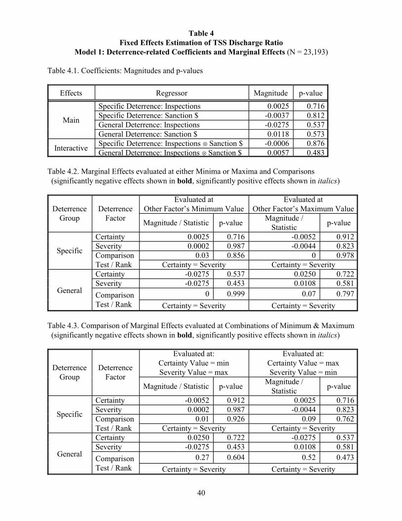
Table 4Fixed Effects Estimation of TSS Discharge Ratio

Model 1: Deterrence-related Coefficients and Marginal Effects (N = 23,193)

Table 4.1. Coefficients: Magnitudes and p-values

Effects Regressor Magnitude p-value

Main

Specific Deterrence: Inspections 0.0025 0.716Specific Deterrence: Sanction $ -0.0037 0.812General Deterrence: Inspections -0.0275 0.537General Deterrence: Sanction $ 0.0118 0.573

InteractiveSpecific Deterrence: Inspections q Sanction $ -0.0006 0.876General Deterrence: Inspections q Sanction $ 0.0057 0.483

Table 4.2. Marginal Effects evaluated at either Minima or Maxima and Comparisons (significantly negative effects shown in bold, significantly positive effects shown in italics)

DeterrenceGroup

DeterrenceFactor

Evaluated atOther Factor’s Minimum Value

Evaluated atOther Factor’s Maximum Value

Magnitude / Statistic p-valueMagnitude /

Statisticp-value

Specific

Certainty 0.0025 0.716 -0.0052 0.912Severity 0.0002 0.987 -0.0044 0.823ComparisonTest / Rank

0.03 0.856 0 0.978Certainty = Severity Certainty = Severity

General

Certainty -0.0275 0.537 0.0250 0.722Severity -0.0275 0.453 0.0108 0.581

ComparisonTest / Rank

0 0.999 0.07 0.797

Certainty = Severity Certainty = Severity

Table 4.3. Comparison of Marginal Effects evaluated at Combinations of Minimum & Maximum (significantly negative effects shown in bold, significantly positive effects shown in italics)

DeterrenceGroup

DeterrenceFactor

Evaluated at:Certainty Value = minSeverity Value = max

Evaluated at:Certainty Value = maxSeverity Value = min

Magnitude / Statistic p-valueMagnitude /

Statisticp-value

Specific

Certainty -0.0052 0.912 0.0025 0.716Severity 0.0002 0.987 -0.0044 0.823ComparisonTest / Rank

0.01 0.926 0.09 0.762Certainty = Severity Certainty = Severity

General

Certainty 0.0250 0.722 -0.0275 0.537Severity -0.0275 0.453 0.0108 0.581

ComparisonTest / Rank

0.27 0.604 0.52 0.473

Certainty = Severity Certainty = Severity

40

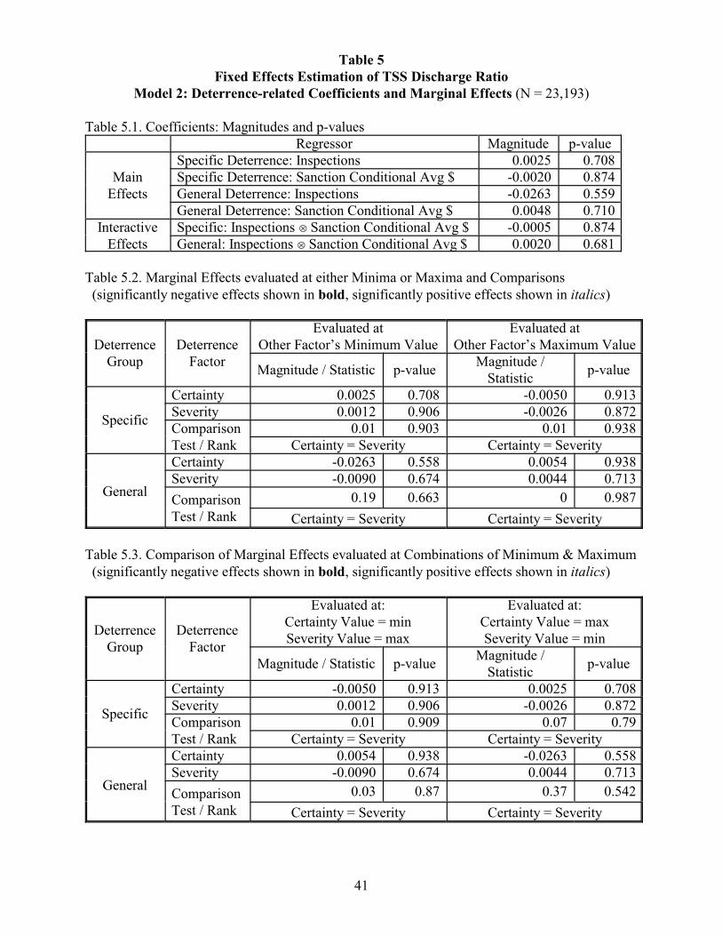
Table 5Fixed Effects Estimation of TSS Discharge Ratio

Model 2: Deterrence-related Coefficients and Marginal Effects (N = 23,193)

Table 5.1. Coefficients: Magnitudes and p-valuesRegressor Magnitude p-value

MainEffects

Specific Deterrence: Inspections 0.0025 0.708Specific Deterrence: Sanction Conditional Avg $ -0.0020 0.874General Deterrence: Inspections -0.0263 0.559General Deterrence: Sanction Conditional Avg $ 0.0048 0.710

InteractiveEffects

Specific: Inspections q Sanction Conditional Avg $ -0.0005 0.874General: Inspections q Sanction Conditional Avg $ 0.0020 0.681

Table 5.2. Marginal Effects evaluated at either Minima or Maxima and Comparisons (significantly negative effects shown in bold, significantly positive effects shown in italics)

DeterrenceGroup

DeterrenceFactor

Evaluated atOther Factor’s Minimum Value

Evaluated atOther Factor’s Maximum Value

Magnitude / Statistic p-valueMagnitude /

Statisticp-value

Specific

Certainty 0.0025 0.708 -0.0050 0.913Severity 0.0012 0.906 -0.0026 0.872ComparisonTest / Rank

0.01 0.903 0.01 0.938Certainty = Severity Certainty = Severity

General

Certainty -0.0263 0.558 0.0054 0.938Severity -0.0090 0.674 0.0044 0.713

ComparisonTest / Rank

0.19 0.663 0 0.987

Certainty = Severity Certainty = Severity

Table 5.3. Comparison of Marginal Effects evaluated at Combinations of Minimum & Maximum (significantly negative effects shown in bold, significantly positive effects shown in italics)

DeterrenceGroup

DeterrenceFactor

Evaluated at:Certainty Value = minSeverity Value = max

Evaluated at:Certainty Value = maxSeverity Value = min

Magnitude / Statistic p-valueMagnitude /

Statisticp-value

Specific

Certainty -0.0050 0.913 0.0025 0.708Severity 0.0012 0.906 -0.0026 0.872ComparisonTest / Rank

0.01 0.909 0.07 0.79Certainty = Severity Certainty = Severity

General

Certainty 0.0054 0.938 -0.0263 0.558Severity -0.0090 0.674 0.0044 0.713

ComparisonTest / Rank

0.03 0.87 0.37 0.542

Certainty = Severity Certainty = Severity

41

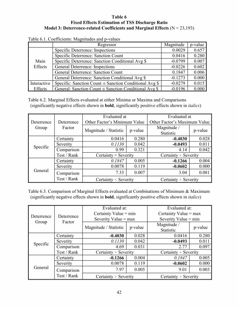
Table 6Fixed Effects Estimation of TSS Discharge Ratio

Model 3: Deterrence-related Coefficients and Marginal Effects (N = 23,193)

Table 6.1. Coefficients: Magnitudes and p-valuesRegressor Magnitude p-value

MainEffects

Specific Deterrence: Inspections 0.0029 0.657Specific Deterrence: Sanction Count 0.0416 0.280Specific Deterrence: Sanction Conditional Avg $ -0.0799 0.007General Deterrence: Inspections -0.0226 0.602General Deterrence: Sanction Count 0.1847 0.006General Deterrence: Sanction Conditional Avg $ -0.1273 0.000

InteractiveEffects

Specific: Sanction Count q Sanction Conditional Avg $ -0.0279 0.015General: Sanction Count q Sanction Conditional Avg $ -0.0196 0.000

Table 6.2. Marginal Effects evaluated at either Minima or Maxima and Comparisons (significantly negative effects shown in bold, significantly positive effects shown in italics)

DeterrenceGroup

DeterrenceFactor

Evaluated atOther Factor’s Minimum Value

Evaluated atOther Factor’s Maximum Value

Magnitude / Statistic p-valueMagnitude /

Statisticp-value

Specific

Certainty 0.0416 0.280 -0.4030 0.028Severity 0.1130 0.042 -0.0493 0.011ComparisonTest / Rank

0.99 0.321 4.14 0.042Certainty = Severity Certainty � Severity

General

Certainty 0.1847 0.005 -0.1266 0.004Severity 0.0078 0.119 -0.0602 0.000

ComparisonTest / Rank

7.33 0.007 3.04 0.081

Certainty � Severity Certainty � Severity

Table 6.3. Comparison of Marginal Effects evaluated at Combinations of Minimum & Maximum (significantly negative effects shown in bold, significantly positive effects shown in italics)

DeterrenceGroup

DeterrenceFactor

Evaluated at:Certainty Value = minSeverity Value = max

Evaluated at:Certainty Value = maxSeverity Value = min

Magnitude / Statistic p-valueMagnitude /

Statisticp-value

Specific

Certainty -0.4030 0.028 0.0416 0.280Severity 0.1130 0.042 -0.0493 0.011ComparisonTest / Rank

4.69 0.031 2.77 0.097Certainty � Severity Certainty � Severity

General

Certainty -0.1266 0.004 0.1847 0.005Severity 0.0078 0.119 -0.0602 0.000

ComparisonTest / Rank

7.97 0.005 9.01 0.003

Certainty � Severity Certainty � Severity

42

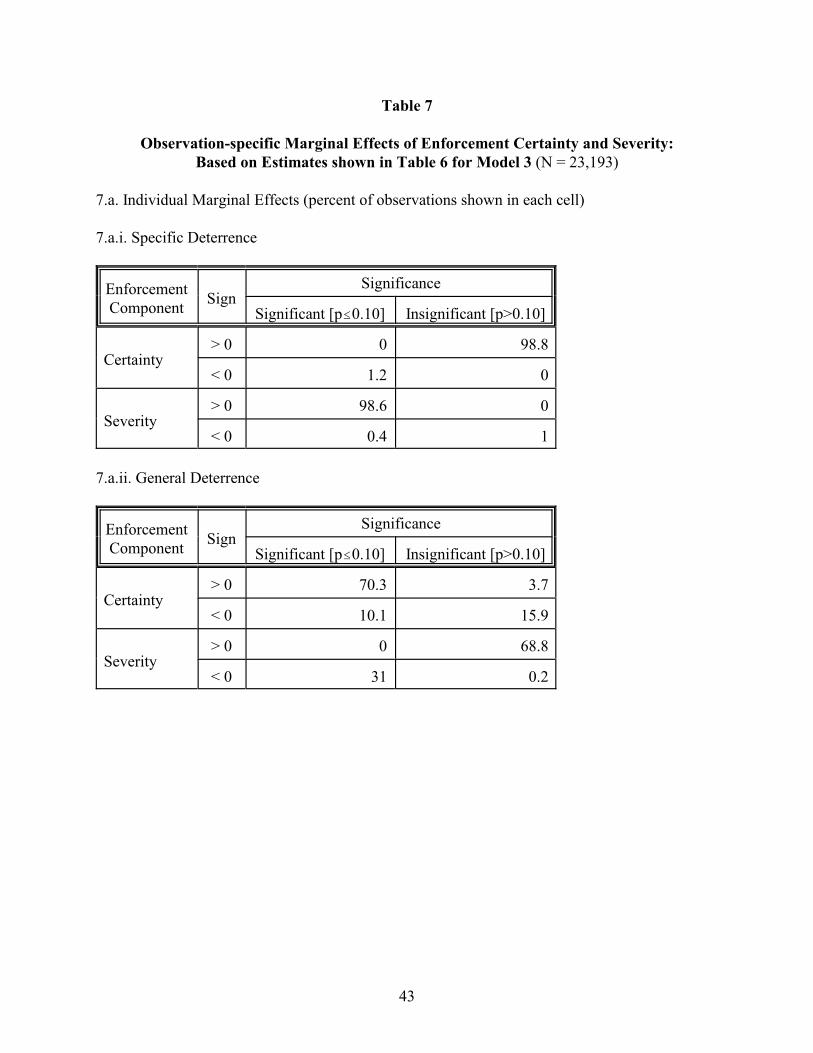
Table 7

Observation-specific Marginal Effects of Enforcement Certainty and Severity:Based on Estimates shown in Table 6 for Model 3 (N = 23,193)

7.a. Individual Marginal Effects (percent of observations shown in each cell)

7.a.i. Specific Deterrence

EnforcementComponent

SignSignificance

Significant [p#0.10] Insignificant [p>0.10]

Certainty> 0 0 98.8

< 0 1.2 0

Severity> 0 98.6 0

< 0 0.4 1

7.a.ii. General Deterrence

EnforcementComponent

SignSignificance

Significant [p#0.10] Insignificant [p>0.10]

Certainty> 0 70.3 3.7

< 0 10.1 15.9

Severity> 0 0 68.8

< 0 31 0.2

43

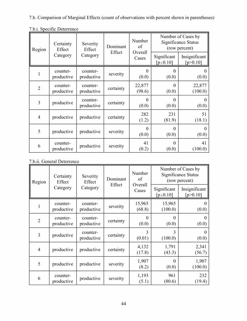
7.b. Comparison of Marginal Effects (count of observations with percent shown in parentheses)

7.b.i. Specific Deterrence

RegionCertainty

EffectCategory

SeverityEffect

Category

DominantEffect

Numberof

OverallCases

Number of Cases bySignificance Status

(row percent)

Significant[p#0.10]

Insignificant[p>0.10]

1counter-

productivecounter-

productiveseverity

0(0.0)

0(0.0)

0(0.0)

2counter-

productivecounter-

productivecertainty

22,877(98.6)

0(0.0)

22,877(100.0)

3 productivecounter-

productivecertainty

0(0.0)

0(0.0)

0(0.0)

4 productive productive certainty282

(1.2)231

(81.9)51

(18.1)

5 productive productive severity0

(0.0)0

(0.0)0

(0.0)

6counter-

productiveproductive severity

41(0.2)

0(0.0)

41(100.0)

7.b.ii. General Deterrence

RegionCertainty

EffectCategory

SeverityEffect

Category

DominantEffect

Numberof

OverallCases

Number of Cases bySignificance Status

(row percent)

Significant[p#0.10]

Insignificant[p>0.10]

1counter-

productivecounter-

productiveseverity

15,965(68.8)

15,965(100.0)

0(0.0)

2counter-

productivecounter-

productivecertainty

0(0.0)

0(0.0)

0(0.0)

3 productivecounter-

productivecertainty

3(0.01)

3(100.0)

0(0.0)

4 productive productive certainty4,132(17.8)

1,791(43.3)

2,341(56.7)

5 productive productive severity1,907(8.2)

0(0.0)

1,907(100.0)

6counter-

productiveproductive severity

1,193(5.1)

961(80.6)

232(19.4)

44

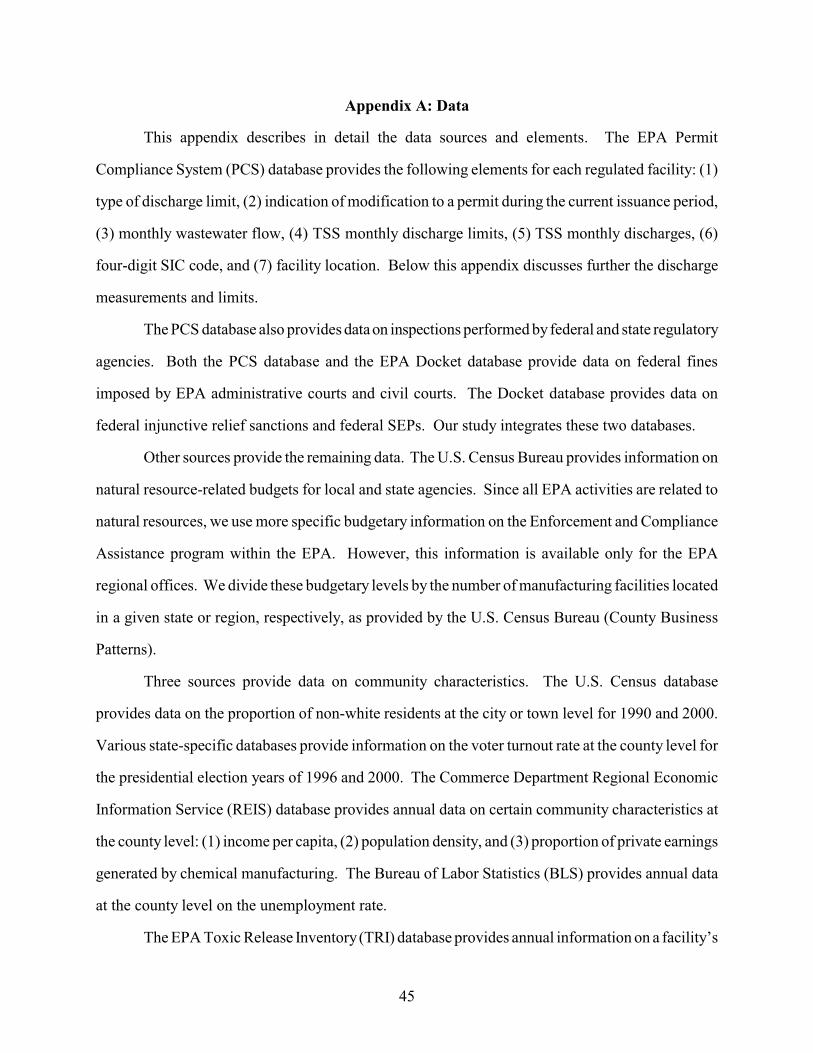
Appendix A: Data

This appendix describes in detail the data sources and elements. The EPA Permit

Compliance System (PCS) database provides the following elements for each regulated facility: (1)

type of discharge limit, (2) indication of modification to a permit during the current issuance period,

(3) monthly wastewater flow, (4) TSS monthly discharge limits, (5) TSS monthly discharges, (6)

four-digit SIC code, and (7) facility location. Below this appendix discusses further the discharge

measurements and limits.

The PCS database also provides data on inspections performed by federal and state regulatory

agencies. Both the PCS database and the EPA Docket database provide data on federal fines

imposed by EPA administrative courts and civil courts. The Docket database provides data on

federal injunctive relief sanctions and federal SEPs. Our study integrates these two databases.

Other sources provide the remaining data. The U.S. Census Bureau provides information on

natural resource-related budgets for local and state agencies. Since all EPA activities are related to

natural resources, we use more specific budgetary information on the Enforcement and Compliance

Assistance program within the EPA. However, this information is available only for the EPA

regional offices. We divide these budgetary levels by the number of manufacturing facilities located

in a given state or region, respectively, as provided by the U.S. Census Bureau (County Business

Patterns).

Three sources provide data on community characteristics. The U.S. Census database

provides data on the proportion of non-white residents at the city or town level for 1990 and 2000.

Various state-specific databases provide information on the voter turnout rate at the county level for

the presidential election years of 1996 and 2000. The Commerce Department Regional Economic

Information Service (REIS) database provides annual data on certain community characteristics at

the county level: (1) income per capita, (2) population density, and (3) proportion of private earnings

generated by chemical manufacturing. The Bureau of Labor Statistics (BLS) provides annual data

at the county level on the unemployment rate.

The EPA Toxic Release Inventory (TRI) database provides annual information on a facility’s

45

parent company. The Business and Company Resource Center database and Compustat / Research

Insight database provide annual data on a parent company’s ownership structure.

All dollar-denominated values are deflated to 1995 levels using the Consumer Price Index.

Lastly, this appendix discusses aspects of discharges and limits. Effluent limits restrict

discharges according to two pollution measures: monthly average and monthly maximum.

Conversations with government officials and the EPA’s definition of significant noncompliance,

however, suggest that regulators primarily care about the average limit (GAO, 1996). Thus, we focus

on the average limit. In addition, effluent limits may restrict only quantities (e.g., pounds of TSS per

day), only concentrations (e.g., milligrams of TSS per liter of water), or both. By focusing on

relative discharges, we are able to compare across all facilities regardless of the effluent limit form.

If both quantity and concentration limits apply, the analysis calculates the mean level of compliance.

(When constructing the effluent limit regressor, we convert each concentration limit to a quantity

limit using the facility’s flow of wastewater.)

Appendix B: Instrumental Variables Estimation

This appendix describes how our study addresses the potential endogeneity of the specific

deterrence regressors by employing a fixed effects instrumental variables (IV) estimator. For this

task, we must identify at least one instrument for each of the potentially endogenous regressors.

Models 1 and 2 include two specific deterrence regressors and Model 3 includes three specific

deterrence regressors. We do not include the interaction term between the enforcement certainty and

severity factors when assessing potential endogeneity for two reasons: (1) assessment of the

underlying factors seems sufficient and (2) assessment of more than three potentially endogenous

regressors is beyond the means of standard statistical tools (Stock and Yogo, 2005).

In order to assess instrument validity, we identify instruments beyond the minimum needed.

In particular, we identify the following instruments: the passage of time since a state agency gained

primacy over the NPDES program and state self-audit policies regarding the privilege of self-

46

discovered violations and immunity from prosecution. Specifically, some states grant immunity28

from prosecution against violations reported to regulatory agencies from facilities who discovered

these violations by conducting self-audits, while other states privilege the evidence of violations

reported to agencies from facilities who conducted self-audits and some states offer both immunity

and privilege. From these possibilities, we construct three separate indicator instruments, with no

policy serving as the benchmark category. Since the specific deterrence regressors measure

inspections and sanctions over a 12-month period yet the state audit policies are recorded for

calendar years, we include both a contemporaneous and a lagged measure of each audit policy

indicator instrument. Thus, we consider seven instruments.

Each of these instruments is theoretically expected to influence regulatory agencies’ decisions

over regulatory interventions but not affect compliance decisions directly. In the case of NPDES

primacy, regulatory “maturity” should influence how inspections are conducted and enforcement

actions are taken. However, conditional on these choices, along with controls for budgetary

resources and EPA regions, no direct effect from regulatory “maturity” to discharge ratios remains.

In the case of state-level audit policies, these policies by federal statute cannot apply to compliance

with wastewater discharge limits since facilities are legally bound to self-report their wastewater

discharges on a regular basis and federal statute excludes use of audit policies in cases where

environmental compliance must be reported.

Effective instrumental variables must satisfy two requirements: they must be correlated with

the included (potentially) endogenous variables, i.e., relevant, and they must be orthogonal to the

error process, i.e., valid (Baum et al., 2003). To assess relevance, we first calculate the partial F-test

statistic, which tests whether the multiple instruments are jointly significant in the estimation of the

potentially endogenous regressors. This estimation represents the first stage of the IV process. For

The EPA provides data on Clean Water Act NPDES primacy on its website. Short and Toffel28

(2010) provide annual data on state-level audit policies. A few states obtained primacy during the sampleperiod; a handful of states had not obtained primacy by the end of the sample period. For those facilitiesoperating in states lacking primacy in a given time period, we code the passage of time as zero. We assesswhether a discontinuity exists at zero. In all cases, our first stage estimates fail to reject the null hypothesisthat no discontinuity exists.

47

Model 1, these partial F-test statistics reveal meaningful relevance given p-values of 0.062 and

0.001, respectively, for the inspection and total sanction monetary value outcomes. For Model 2,

the partial F-test statistics reveal meaningful relevance given p-values of 0.062 and 0.001,

respectively, for the inspection and conditional average sanction magnitude outcomes. For Model

3, these partial F-test statistics reveal sufficient if not meaningful relevance given p-values of 0.097,

0.042, and 0.001, respectively, for the inspection, sanction count, and conditional average sanction

magnitude outcomes. We next test under-identification in the first stage. Based on Kleibergen-Paap

Lagrange Multiplier Test statistics, we reject the null hypothesis of under-identification given p-

values of 0.063, 0.002, and 0.023, respectively, for Models 1, 2, and 3.

To assess the validity of our instruments, we employ the Hansen J Test of Overidentifying

Restrictions. The test statistics fail to reject the null hypothesis of valid orthogonality conditions

given p-values of 0.129, 0.101, and 0.162, for Models 1, 2, and 3. Thus, our instruments do not29

appear invalid. Nevertheless, we acknowledge that the reported p-values nearly reveal that our

instruments might not be valid.

Based on our assessment, the instruments appear both relevant and not invalid. Therefore,

we proceed to testing whether the potentially endogenous regressors are exogenous using a Durbin-

Wu-Hausman Exogeneity Test. The test statistics fail to reject the null hypothesis of exogeneity

given p-values of 0.573, 0.621, and 0.343, respectively, for Models 1, 2, and 3. These statistics

indicate that the specific deterrence regressors do not appear endogenous. Performing IV estimation

when the regressors are uncorrelated with the error process involves an important cost – “the

asymptotic variance of the IV estimator is always larger, and sometimes much larger, than the

asymptotic variance of the OLS estimator” (Wooldridge, 2002, p. 490). Therefore, we proceed with

the standard fixed effects estimator when estimating the functional relationship between the

discharge ratio and various regressor sets.

Our assessment of the exogeneity regarding specific deterrence factors represents a

Technically, this test assesses the joint hypothesis of correct model specification and valid29

orthogonality conditions; see Baum et al. (2003) on this point.

48

contribution to the literature since no previous study addresses the potential endogeneity to any

meaningful extent. This appendix describes previous studies treatment of specific deterrence factors.

Several studies treat lagged measures of inspections as exogenous regressors (Magat and Viscusi,

1990; Helland, 1998a; Helland, 1998b). Other studies treat lagged measures of government

interventions as exogenous even while addressing the endogeneity of current measures. For

example, Gray and Deily (1996) explore the specific deterrence generated by inspections alone and

the combination of inspections and informal enforcement actions. In this exploration, the authors

employ lagged measures while implicitly treating them as exogenous. When employing

contemporaneous measures of these government interventions, the authors use a two-stage

estimation that first predicts the extent of current monitoring and informal enforcement. Laplante

and Rilstone (1996) employ a similar approach when exploring the effects of inspections. The

authors first include only lagged measures and then only a predicted current measure. Lastly,

Shimshack and Ward (2008) explore specific deterrence effects by employing lagged measures of

fines (in monetary terms) and inspections, while claiming that fixed effects estimation handles any

potential targeting of enforcement. However, this claim does not hold if targeting varies over time,

which is most likely true.

49

REFERENCES

Anderson, Lisa R. and Sarah L. Stafford (2003), "Punishment in a Regulatory Setting: Experimental

Evidence from the VCM," Journal of Regulatory Economics, 24(1), pg. 91-110.

Arora, Seema and Timothy Cason (1996), “Why Do Firms Volunteer to Exceed Environmental

Regulations? Understanding Participation in EPA’s 33/50 Program,” Land Economics, 72

(4), pg. 413-432.

Bandyopadhyay, Sushenjit and John Horowitz (2006), "Do Plants Overcomply with Water Pollution

Regulations? The Role of Discharge Variability," B.E. Journal of Economic Analysis and

Policy: Topics in Economic Analysis and Policy, 6(1), pg. 1-32.

Baum, Christopher, Mark Schaffer, and S. Stillman (2003), “Instrumental Variables and GMM:

Estimation and Testing,” Stata Journal, 3, pg. 1-31.

Becker, Gary S. (1968), "Crime and Punishment: An Economic Approach," Journal of Political

Economy, 76, pg. 169-217.

Cohen, Mark (2000), “Empirical Research on the Deterrent Effect of Environmental Monitoring and

Enforcement,” Environmental Law Reporter, 30, pg. 10245-10252.

Croson, R., and Sundali, J. (2005), "The Gambler's Fallacy and the Hot Hand: Empirical Data from

Casinos," Journal of Risk and Uncertainty, 30, 195-209.

Dasgupta, Susmita, Hemamala Hettige and David Wheeler (2000), “What Improves Environmental

Compliance? Evidence from Mexican Industry,” Journal of Environmental Economics and

Management, 39, pg. 39-66.

Downing, P. and J. Kimball (1982), “Enforcing Pollution Control Laws in the United States,” Policy

Studies Journal, 11 (1), pg. 15-22.

Earnhart, Dietrich (2004a), “Panel Data Analysis of Regulatory Factors Shaping Environmental

50

Performance,” Review of Economics and Statistics, 86 (1), pg. 391-401.

Earnhart, Dietrich (2004b), “Regulatory Factors Shaping Environmental Performance at Publicly-

Owned Treatment Plants,” Journal of Environmental Economics and Management, 48 (1),

pg. 655-681.

Earnhart, Dietrich (2004c), “The Effects of Community Characteristics on Polluter Compliance

Levels,” Land Economics, 80 (3), pg. 408-432.

Earnhart, Dietrich (2009), “The Influence of Facility Characteristics and Permit Conditions on the

Effects of Environmental Regulatory Deterrence,” Journal of Regulatory Economics, 36 (3),

pg. 247-273.

Earnhart, Dietrich and Lana Friesen (2013), “Can Punishment Generate Specific Deterrence without

Updating? Analysis of a Stated Choice Scenario,” Environmental and Resource Economics,

56 (3), pg. 379-397.

Earnhart, Dietrich and Robert Glicksman (2011), Pollution Limits and Polluters’ Efforts to Comply:

The Role of Government Monitoring and Enforcement, Palo Alto, CA: Stanford Univ Press.

Earnhart, Dietrich and Kathleen Segerson (2012), “The Influence of Financial Status on the

Effectiveness of Environmental Enforcement,” Journal of Public Economics, 96, pg. 670-

684.

Earnhart, Dietrich and Robert Glicksman (2013), “Coercive vs. Cooperative Enforcement: Effect

of Enforcement Approach on Environmental Management,” University of Kansas working

paper.

Eckert, Heather (2004), “Inspections, Warnings, and Compliance: The Case of Petroleum Storage

Regulation,” Journal of Environmental Economics and Management, 47 (2), pg. 232-259.

Eide, Erling (2000), Economics of Criminal Behavior, in Encyclopedia of Law and Economics,

51

Boudewijn Bouckaert and Gerrit De Geest (eds), Cheltenham: Edward Elgar.

Eide, Erling, P.H. Rubin, and J.M. Shepherd (2006), "Economics of Crime," Foundations and

Trends in Microeconomics, 2, pg. 205-279.

EPA (1990), “A Primer on the Office of Water Enforcement and Permits and Its Programs,” Office

of Water, Environmental Protection Agency, Washington, DC, March 1990.

EPA (1997), Chemical Industry National Environmental Baseline Report 1990-1994, Office of

Enforcement and Compliance Assurance, Environmental Protection Agency, EPA 305-R-96-

002, October 1997.

EPA (1999a), EPA/CMA Root Cause Analysis Pilot Project: An Industry Survey, Environmental

Protection Agency, EPA-305-R-99-001, May 1999.

EPA (1999b), “Major Findings from the CEIS Review of EPA’s Permit Compliance System

Database,” EPA Center for Environmental Information and Statistics (CEIS), Washington,

DC.

EPA (2011), Technical Support Document for the 2010 Effluent Guidelines Program Plan,

Environmental Protection Agency, EPA 820-R-10-021.

Fehr, E. and A. Falk (2002), "Psychological Foundations of Incentives," European Economic

Review, 46, pg. 687-724.

Foulon, Jérôme, Paul Lanoie and Benôit Laplante (2002), “Incentives for Pollution Control:

Regulation or Information,” Journal of Environmental Economics and Management, 44 (1),

pg. 169-187.

Frey, B.S. and R. Jegen (2001), "Motivation Crowding Theory," Journal of Economic Surveys, 15,

pg. 589-611.

Friesen, Lana (2012), “Certainty of Punishment versus Severity of Punishment: An Experimental

52

Investigation,” Southern Economic Journal, 79 (2), pg. 399-421.

GAO (1996), “Water Pollution: Many Violations Have Not Received Appropriate Enforcement

Attention,” General Accounting Office, Report # GAO/RCED-96-23, Washington, DC.

Gneezy, U., S. Meier, and P. Rey-Biel (2011), “When and Why Incentive (Don’t) Work to Modify

Behavior,” Journal of Economic Perspectives, 25 (4), pg. 191-210.

Gray, Wayne B. and Mary E. Deily (1996), "Compliance and Enforcement: Air Pollution Regulation

in the U.S. Steel Industry," J. of Environmental Economics and Management, 31, pg. 96-111.

Gray, Wayne and John Scholz (1991), "Analysing the Equity and Efficiency of Osha Enforcement,"

Law & Policy, 13, pg. 185-214.

Gray, Wayne and John Scholz (1993), "Does Regulatory Enforcement Work? A Panel Analysis of

OSHA Enforcement," Law & Society Review, 27, pg. 177-213.

Gray, Wayne B. and Ronald J. Shadbegian (2004), "'Optimal' Pollution Abatement - Whose Benefits

Matter, and How Much?," Journal of Environmental Economics and Management, 47, pg.

510-534.

Gray, Wayne B. and Ronald J. Shadbegian (2005), “When and Why do Plants Comply? Paper Mills

in the 1980s,” Law and Policy, 27 (2), pg. 238-261.

Gray, Wayne B., and Jay P. Shimshack (2011), "The Effectiveness of Environmental Monitoring and

Enforcement: A Review of the Empirical Evidence," Review of Environmental Economics

and Policy, 5, pg. 3-24.

Grogger, J. (1991) "Certainty vs. Severity of Punishment", Economic Inquiry, 29 (2), pg. 297-309.

Hamilton, James (1993), “Politics and Social Costs: Estimating the Impact of Collective Action on

Hazardous Waste Facilities,” RAND Journal of Economics, 24 (1), pg. 101-125.

Helland, Eric (1998a), “The Enforcement of Pollution Control Laws: Inspections, Violations and

53

Self-Reporting,” Review of Economics and Statistics, 80 (1), pg. 141-153.

Helland, Eric (1998b), “The Revealed Preferences of State EPAs: Stringency, Enforcement, and

Substitution,” Journal of Environmental Economics and Management, 35 (3), pg. 242-261.

Helland, Eric and Andrew Whitford (2003), "Pollution Incidence and Political Jurisdiction:

Evidence from the TRI," Journal of Environmental Economics and Management, 46, pg.

403-424.

Heyes, Anthony and S. Kapur (2009), "Enforcement Missions: Targets vs Budgets," Journal of

Environmental Economics and Management, 58, pg. 129-140.

Henriques, Irene and Perry Sadorsky (1996), “The Determinants of an Environmentally Responsive

Firm: An Empirical Approach,” Journal of Environmental Economics and Management, 30,

pg. 381-395.

Laplante, Benoît and Paul Rilstone (1996), “Environmental Inspections and Emissions of the Pulp

and Paper Industry in Quebec,” Journal of Environmental Economics and Management, 31

(1), pg. 19-36.

Magat, Wesley A. and W. Kip Viscusi (1990), “Effectiveness of the EPA’s Regulatory Enforcement:

The Case of Industrial Effluent Standards,” Journal of Law and Economics, 33 (2), pg. 331-

360.

Nadeau, Louis W. (1997), “EPA Effectiveness at Reducing the Duration of Plant-Level

Noncompliance,” Journal of Environmental Economics and Management, 34 (1), pg. 54-78.

Polinsky, A. Mitchell and Steven Shavell (2000), "The Economic Theory of Public Enforcement of

Law," Journal of Economic Literature, 38, pg. 45-76.

Sah, Raj K. (1991), "Social Osmosis and Patterns of Crime," Journal of Political Economy, 99, pg.

1272-1295.

54

Scholz, John T. and Wayne B. Gray (1990), "Osha Enforcement and Workplace Injuries: A

Behavioral Approach to Risk Assessment," Journal of Risk and Uncertainty, 3, pg. 283-305.

Shimshack, Jay P. and Michael B. Ward (2005), "Regulator Reputation, Enforcement, and

Environmental Compliance," Journal of Environmental Economics and Management, 50,

pg. 519-540.

Shimshack, Jay P. and Michael B. Ward (2008), "Enforcement and over-Compliance," Journal of

Environmental Economics and Management, 55, pg. 90-105.

Short, Jodi and Michael Toffel (2010), "Making Self-Regulation More Than Merely Symbolic: The

Critical Role of the Legal Environment," Administrative Science Quarterly, 55, pg. 361-396.

Sigman, Hilary (1998), “Midnight Dumping: Public Policies and Illegal Disposal of Used Oil,”

RAND Journal of Economics, 29 (Spring), pg. 157–178.

Stock, J. and M. Yogo (2005), “Testing for Weak Instruments in Linear IV Regression,” in

Identification and Inference for Econometric Models: Essays in Honor of Thomas

Rothenberg, eds. D.W.K. Andrews and J.H. Stock, pg. 80-108, New York: Cambridge

University Press.

Tversky, Amos and Daniel Kahneman (1974), "Judgment under Uncertainty: Heuristics and Biases,"

Science, 185, pg. 1124-1131.

Wasserman, Cheryl (1984), “Improving the Efficiency and Effectiveness of Compliance Monitoring

and Enforcement of Environmental Policies, United States: A National Review,” OECD.

Winter, S.C. and Peter J. May (2001), "Motivation for Compliance with Environmental

Regulations," Journal of Policy Analysis and Management, 20, pg. 675-698.

Wooldridge, Jeffrey (2002), Econometric Analysis of Cross Section and Panel Data, MIT Press:

Cambridge, MA.

55

Figu

re 1

: Est

imat

ed M

argi

nal E

ffec

ts w

ith r

espe

ct to

Cer

tain

ty a

nd S

ever

ity in

clud

ing

90%

Con

fiden

ce In

terv

als

-.8-.6-.4-.20.2Marginal Effect

014

722

,000

3.3m

Sev

erity

Spe

cific

Det

erre

nce:

Cer

tain

ty

-.8-.6-.4-.20.2Marginal Effect

00.

002

0.00

60.

020.

050.

130.

37C

erta

inty

Spe

cific

Det

erre

nce:

Sev

erity

-.20.2.4Marginal Effect

014

722

,000

3.3m

Sev

erity

Gen

eral

Det

erre

nce:

Cer

tain

ty

-.20.2.4Marginal Effect

00.

002

0.00

60.

020.

05C

erta

inty

Gen

eral

Det

erre

nce:

Sev

erity

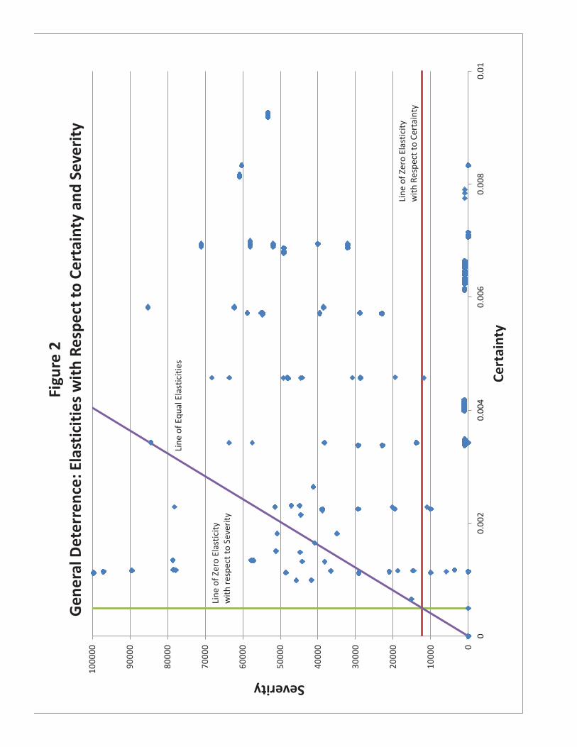
0

1000

0

2000

0

3000

0

4000

0

5000

0

6000

0

7000

0

8000

0

9000

0

1000

00

00.

002

0.00

40.

006

0.00

80.

01

Severity

Cert

aint

y

Figu

re 2

Ge

nera

l Det

erre

nce:

Ela

stic

ities

with

Res

pect

to C

erta

inty

and

Sev

erity

Line

of Z

ero

Elas

ticity

w

ith R

espe

ct to

Cer

tain

ty

Line

of Z

ero

Elas

ticity

w

ith re

spec

t to

Seve

rity

Line

of E

qual

Ela

stic

ities