Default and Punishment: Incentives and Lending Behavior in

Indian Banks

Abhijit Banerjee, Shawn Cole, Esther Du�o�

February 2009y

Abstract

We analyze a model of lending in which loan o¢ cers face both an incentive to lend, and

possible penalties for loans that go bad. The model predicts the following: new �rms will

face credit constraints; if the penalty does not increase proportionally with the volume of

default, loan o¢ cers will have an incentive to �evergreen,� i.e. bail out failed borrower when

the probability of being punished for default increases. We test these predictions using a

dataset of all commercial bank loans in India from 1981 to 2003, combined with a data set

on the investigation and discovery of fraud by the �central vigilance commission", a federal

body charged with investigating default. We �nd evidence that following the discovery of a

fraud in a particular bank branch, vigilance activities greatly increases. This in turn results

in reduced lending: the amount of credit declines sharply at the a¤ected bank branch, as

well as neighboring branches. This e¤ect is large, and persists in part for up to two years.

Bank risk-taking also declines following an inspection.

�MIT (banerjee@mit.edu), Harvard Business School (scole@hbs.edu), and MIT (edu�o@mit.edu), respectively.yWe thank Raghuram Rajan, with whom a conversation many years ago prompted us to undertake this project.

This work is a collaborative exercise with research sta¤ from the Reserve Bank of India, including S. Majumdar,

Deepak Gogia, and Janak Raj. The RBI performed much of the statistical analysis in this paper. The statements

made in this paper do not in any way represent the view of the Reserve Bank of India or its employees. We thank

seminar participants at Harvard Business School, NEUDC, MIT, George Washington, and Maryland.

1

1 Introduction

Standard neo-classical theory predicts that interest rates alone should predict the supply of

bank credit, and that the expected risks and returns of various projects and borrowers should

determine its allocation. In part because of the need to spread idiosyncratic risk, banks are

often large organizations, which makes providing incentives to loan o¢ cers to collect and reveal

information about the borrowers inherently di¢ cult. How banks solve these incentives problems

can have fundamental consequences on how capital is allocated in the economy.

Several studies have shown that organizational issues within banks do indeed a¤ect

the volume and the nature of lending. Berger, Demsetz and Strahan (1999) show that after

consolidations, banks are less likely to lend to small businesses and Stein (2002) argues that this

phenomenon is due to the di¢ culty of providing incentives to gather and truthfully reveal �soft"

information within large banks. Hertzberg, Liberti and Paravisini (2007) further investigate

the role of incentives to provide information within banks. They show that rotation of o¢ cers

alleviates the temptation by loan o¢ cers not to reveal bad news about the �rms they deal with.

The fundamental problem that banks face is that they need to provide incentives to their

employees, who are paid a fraction of the money they have to manage, both to exert e¤ort to

�nd clients to lend to, and to avoid default. These two objectives are however likely to con�ict

since the easiest way to avoid a default is not to lend at all.

In this paper we study theoretically and empirically, the impact of how loan o¢ cers are

punished for defaulting on the volume and the nature of their lending decisions. Incentives to

prevent default are necessary to induce loan o¢ cers to lend to pro�table projects, to monitor

their clients, and to refrain from stealing money. But they may also discourage honest loan

o¢ cers to lend. And if the punishment does not sharply increase with the size of the default, an

increase in the probability of being punished may also encourage �evergreening", or �gambling

for revival": lending to �rms which are about to default in the hope that they will receive a

good draw in the next period and get out of their bad situation.1

Our empirical setting is the sector in India, which has long been dominated by government-

owned banks. Public banks have limited availability to provide incentives to loan o¢ cers: wages

1Rajan (1994) develops a model where these types of behavior is undertaken by loan o¢ cer to protect their

reputation.

2

increase mainly with seniority, and it is di¢ cult to �re employees. The main instrument for the

bank to punish a loan o¢ cer is to transfer him to an undesirable posting. However, the risk of

corruption is a key concern to the government and, to alleviate it, loans o¢ cers are subject to

the government anti-corruption laws. In particular, a bad loan may in principle be treated as

embezzlement of government funds, and thus lead to a criminal investigation. A federal body,

the Central Vigilance Commission, investigates a small fraction of suspected frauds. While in-

vestigations are rare, and convictions even rarer, bankers argue that the risk of being charged

with corruption is a �sword of Damocles" hanging above their heads and preventing them from

making reasonable decisions.

In this context, we study what happens when the probability of being investigated by

the vigilance commission increases. To do so, we exploit an unusual data set, made available

at the Reserve Bank of India. The data set contains information (date, type, location, and

punishment) on all the frauds reported to the Reserve Bank of India between 1980 and 2006.

We use it in conjunction with quarterly and annual information on lending at the branch level

for a panel of over 43,000 bank branches in the country followed for several years.

We start by showing that when a fraud is discovered by the Central Vigilance Commission

in a particular branch in a particular year, the discovery of other frauds in the same branch

increases by a factor of 27 in that year, compared to previous years. This suggests a clear

persistence in vigilance activity: the probability of being punished for default is larger in a

bank branch in the year following the investigation of a fraud. We exploit this within an event-

study approach, where we study how lending behavior in a particular branch changes after

the discovery of a fraud in the years following the discovery, compared to other branches. We

�nd a rapid and persistent drop in credit at the a¤ected branch, which cumulates to at least

a 20% decline in lending. This decline is driven by a decline in high-quality loans, and we

�nd suggestive evidence of ever-greening. Vigilance activity also a¤ects the sectoral allocation

of credit, as branches shift credit from riskier to less risky sectors. Finally, vigilance activity

a¤ects other branches of the same bank in the same town.

These results echo those in Banerjee and Du�o (2008), which exploit a shock to the

availability of subsidized credit to a subset of �rms in India, and �nd evidence that even fairly

large �rms with an existing relationship to the banking sector are severely credit constrained.

3

These results also indicate substantial misallocation of credit by loan o¢ cers: the average rupee

lent has a much lower return than the extra credit induced by the program; there seems to

be no relationship between performance and increment in the lending limit. By showing that

corruption has an indirect negative e¤ect on the volume and the allocation of credit in an

economy, through its e¤ect on the honest agents who are worried about being punished, they

also help explain the large impact of corruption on lending, found for example in Beck, Demirguc-

Kunt and Levine (2006).

The remainder of this paper proceeds as follows. In Section 2 we provide a brief descrip-

tion of banking in India, and a discussion of the debate on the relationship between corruption

and lending. We develop a model of the loan allocation decision by a honest agent subject

to incentives to lend and to avoid default in section 3, and describe the data in the following

section. We then use the data to learn something about the parameters of the model,in Section

5. Finally, section presents the empirical results, testing the model�s predictions about the rela-

tionship between fraud discovery, lending, default, and the riskiness of decisions taken by banks.

Finally, Section 7 concludes.

2 Context and Overview

In this section, we brie�y describe the context in which banks operate, including anecdotal

evidence on the claim that fear of prosecution causes loan o¢ cers to behave very conservatively.

We focus on government-owned banks because they dominate the Indian �nancial system.

Public sector banks include both government founded banks (such as the Bank of India), as well

as banks nationalized by the government in 1969 and 1980. In the 1990s, several formerly public

banks were partially privatized, and foreign banks had entered, primarily in large cities. While

public sector banks market share has declined since then, in 2006 government-owned banks

provided 71% of bank credit in the economy.

Corruption in lending is a major policy concern, in India and elsewhere. Cole (2008)

shows that lending follows a political cycle. Khwaja and Mian (2005) document political cor-

ruption of loans in Pakistan. In India, since public sector banks are owned by the government,

employees of the bank are treated by law as public servants, and thus subject to government

4

anti-corruption rules. In particular, any default is in principle subject to investigation by the

Central Vigilance Commission, a federal authority which maintains an arms-length relationship

with the banks, but is empowered to prosecute loan o¢ cers.

Bankers have expressed concern that it is very easy to be charged with corruption. Some

feel that any �nancial loss to a government owned bank would automatically lead to investigation,

with the burden of proof on the banker to prove her or his innocence. The quote below is fairly

typical.

[Bankers] say that government o¢ cials, who are clueless about banking eco-

nomics, are posted as vigilance o¢ cials and there is the threat of a vigilance inquiry

each time a bona �de lending decision results in a bad account. Bankers say that

they are �ush with funds, but credit is not taking o¤ because of fear psychosis. A

top banker said: "You become averse to risks in such an environment. Many of us

are turning to narrow banking and stick to gilts.2"

The Reserve Bank of India (RBI), the Indian equivalent of the Federal Reserve has also

argued that another result of this fear is bankers reluctance to settle non-performing loans (RBI

2000, p. 29), for fear of being charged with corruption. In 2000, the Indian banking system had

among the highest percentage of assets in default of any banking system in the world.

A working group on banking policy set up by the Reserve Bank of India, and chaired by

M.S. Verma, noted in 2000:

The [working group] observed that it has received representations from the man-

agements and the unions of the banks complaining about the di¢ dence in taking

credit decisions with which the banks are beset at present. This is due to investi-

gations by outside agencies on the accountability of sta¤ in respect of some of the

N[on] P[erforming] A[ssets]. The group also noticed a marked reluctance at various

levels to take any credit decision. (Tannan 2001, p. 1579).

In response to criticism from bankers, economists, and others, the Central Vigilance

Commission introduced in 1999 a special chapter of the vigilance manual, on vigilance in public2Frontline (Hindu), 15(10), May 9-22, 1998. Accessed at http://www.hinduonnet.com/�ine/�1510/15101090.htm

on October 20, 2007.

5

sector banks. While this new chapter was meant to reassure bankers, the language would

probably not reassure anyone with experience working in a multinational bank. The manual

reads, for example, that �every loss caused to the organization, either in pecuniary or non-

pecuniary terms, need not necessarily become the subject matter of a vigilance inquiry. . . once a

vigilance angle is evident, it becomes necessary to determine through an impartial investigation

as to what went wrong and who is accountable for the same.�(p. 5)

Interviews with public sector bankers revealed widespread concern: the legal proceedings

surrounding charges of corruption can drag on for years, leaving individuals charged with cor-

ruption in an uncertain state. Even if an individual is exonerated, she may have been relieved of

her duties, transferred, or passed over for promotion during the time of investigation. In theory

(as well as practice), even one loan gone bad may be su¢ cient to start vigilance proceedings.

The possible penalties stand in stark contrast to rewards. While banks are constantly urged

by the Reserve Bank of India to loan as much as possible, there are no explicit incentives for

making good loans, or ways to penalize o¢ cers who make conservative decisions.

Not surprisingly, the Central Vigilance Commission disputes the claim that there is a

�fear psychoses,�and, to bolster their position, released in 2000 a �critical analysis�of vigilance

activity in public sector banks in 1999. The analysis reveals that in 1999, the Central Vigilance

Commission received 1,916 references, 72% of which were credit-related, of which 55% resulted

in recommendations for major punishment.

Thus, compared to the volume of lending, the probability to be investigated for a fraud

is actually extremely small. Moreover, their 2000 report states "Out of every 100 cases coming

before it, the Commission would advise major penalty proceedings in 28 cases, minor penalty

proceedings in 32 cases, and administrative warning/exoneration in 40 cases." (p. 9). The

author of the report, a CVC o¢ cial, argued that this level of activity should not be enough to

cause �fear psychoses�: �These �gures reveal that a person is not damned the moment his [sic]

case is referred to the Commission...These statistics appear to indicate a very fair and objective

approach on the part of the Commission to the cases that were referred to it.� (CVC 2000 p.

10).

Nevertheless, the �fear of lending" arguments made by the bankers seem to have been

serious enough to convince the government: In April 2004 (after the period covered by this

6

study), lower-level loan o¢ cers were removed from the jurisdiction of the Central Vigilance

Commission. Our data covers the period before this changes, when even low level loan o¢ cers

could still be charged by the CVC.

3 Theory

In this section, we describe a model in which a loan o¢ cer allocates capital to �rms. Loan o¢ cers

are given incentives to lend money and they are punished for default. The model studies how

the shape of the punishment as a function of the default a¤ect a honest loan o¢ cer�s incentive

to lend, and to allocate its lending.

3.1 Model setup

The model examines loan o¢ cer incentives and decisions, taking as exogenous the mix of �rms

available to which to lend. The components of the model are as follows:

Firms: Firms in this economy come in two types�H and L�in proportions p and 1� p:

Their production function is as follows: with probability p(k; �i); where i = L;H; �H > �L

and p(k; �i) is a concave function of k; the �rm produces �k: With probability 1� p(k; �i) the

�rm produces 0. Assume that pk(k; �i) < 0, i.e. bigger projects are more likely to fail, that

p(k; �H) > p(k; �L) which de�nes the type H �rm to be the more productive �rm, and that

0 > pk(k; �H) > pk(k; �L): That is, pk is increasing in �; which derives from the idea that the

better �rm is better able to handle an in�ow of capital. Finally assume that kp(k; �i) is an

increasing but concave function of k:

Firms live for two periods and produce in both�the shock to its productivity is drawn

independently from the same distribution in both periods. Firms do not save and have no equity,

so in each period, production is entirely �nanced by credit and the current output is all they

have to repay any loans. We will assume that there is no �rm-side moral hazard: �rms never

deliberately default. However if they do not have enough money they have no choice but to

default.

Bank: There is a bank that is the sole source of capital to this population of �rms. To

simplify matters we will always assume that banks set a single interest rate r for all loans. The

7

cost of bank capital is � < r: Lending decisions are made by bankers who work for the bank but

maximize their own expected earnings (rather than the bank�s earnings), which in turn are a

function of the incentives that the banks set for them.

Bankers: Each new �rm get allocated to a banker who works with it for the next two

periods. Bankers get paid an amount C per unit they lend. They also get punished for any loans

that they made that were ultimately defaulted upon. The punishment is given by �F (k) where

k is size of the loan, F is an increasing function and � is a shift parameter which distinguishes

between high and low monitoring regimes. The fact that both C and F (k) are taken as being

exogenous is unorthodox. Endogenizing C is relatively straightforward. As far as endogenizing

F is concerned, the fact is that it is determined by the Vigilance Commission, which deliberately

maintains an arms-length relation with the bank. Therefore we should not expect it to be chosen

optimally from the point of the bank. Our strategy therefore is to treat it as a parameter and

examine the e¤ects of shifts in it. Finally we assume that bankers do not discount the future

and maximize expected net bene�ts (i.e. are risk neutral).

Information: In the �rst period neither the �rm nor the banker knows the �rm�s type.

At the end of the �rst period they both observe the �rm�s output and update accordingly using

the fact they both know how much the �rm had invested: Successful �rms are going to be type

H with probability

ps(k) =pp(k; �H)

pp(k; �H) + (1� p)p(k; �L)

Since 0 > pk(k; �H) > pk(k; �L) and p(k; �H) > p(k; �L);p(k;�H)p(k;�L)

is increasing in k, which is why

ps is increasing in k: Likewise the probability that a failed �rm is type H; pf ; is declining in k:

Timing: We will study the case where the current level of monitoring (and hence the

expected punishment) is high, but is expected to go down. In particular assume that a present

level of � > 1; but that it is expected to go down to � = 1 over the next periods. In particular,

the probability that it goes down to 1 in the next period is q and if it does not go down next

period it is certain to go down in the following period. Once it does go down it is expected to

stay there for the foreseeable future. The idea is that the bank is now under scrutiny so that

defaults are highly likely to be investigated, but eventually the Vigilance Commission�s attention

will shift elsewhere and the probability of an investigation will go down.

A banker starts with one population of borrowers who borrowed last period (before �

8

went up) and another population of new borrowers.

3.1.1 Lending to a successful old �rm

Suppose that a �rm is in the second period of its life, was able to repay its �rst period loan and

is of type H with probability p0. Then the amount the banker would want to lend to that �rm

in the second period is given by maximizing

Ck � [p0(1� p(k2; �H)) + (1� p0)(1� p(k2; �L))](q + (1� q)�)F (k)

where we write k2 to remind ourselves that this is the second period. The solution is given by

solving the equation

C = [p0(1� p(k2; �H)) + (1� p0)(1� p(k2; �L))](q + (1� q)�)F 0(k2)

�[p0pk(k2; �H) + (1� p0)pk(k2; �L)](q + (1� q)�)F (k2)

As long as the second order condition for this maximization holds (which we assume),

an increase in p0 will increase k2; because both [p0(1 � p(k2; �H)) + (1 � p0)(1 � p(k2; �L))] and

�[p0pk(k2; �H)+ (1� p0)pk(k2; �L)] go down when p0 goes up. Better borrowers get bigger loans.

Also k2 is declining in q+(1� q)� ; which is the expected value of � ; which we will denote by � e:

More stringent punishments will discourage lending. Hence k2 = k2(p0; � e); with k2p > 0; and

k2�e < 0:

Clearly, for appropriately chosen values of F and C; the amount the banker wants to lend

can be very large, indeed larger than what the �rm wants to borrow. However let us assume

that the opposite is the case in the empirically relevant range� which is consistent with the

evidence in Banerjee and Du�o (2004) showing that clients of the banking system tend to be

credit constrained.

3.2 Lending to a failed old �rm: bailouts

Consider now the alternative case where everything is the same about the �rm except that it has

failed in the �rst period and hence has no output to repay its loan. One thing the banker could

do is to let the �rm declare bankruptcy and then lend to it based on its p0 and the value of �

expected for the next period, i.e. k2(p0; � e): In this case the banker gets a punishment F (k1) for

9

the �rst period default, where k1 was the �rst period loan to the �rm. The alternative is to bail

it out: Give it a loan such that it can repay the �rst period loan (and thereby avoid defaulting)

and as well as the second period loan, if it manages to the successful in period 2. This means a

loan of size kb(k1)

�(kb(k1)� k1r) = kb(k1)r

or kb(k1) =�rk1�� r :

This would avoid immediate default but create a risk of a bigger default in the future (since

r > 1; �r��r > 1). From the banker�s point of view the trade-o¤ is between

�NB(k1; p0; � e; �)

= Ck2(p0; � e)� �F (k1)� � eF (k2(p0; � e)[1� p0p(k2(p0; � e); �H))� (1� p0)p(k2(p0; � e); �L))]

and

�B(k1; p0; � e)

= Ckb(k1)� � eF (kb(k1)[1� p0p(kb(k1)� rk1; �H)� (1� p0)p(kb(k1)� rk1; �L)]

Denoting by 1� p0p(k; �H))� (1� p0)p(k; �L) = �(k; p0), bailouts dominate if

�F (k1) (1)

� fCk2(p0; � e)� � eF (k2(p0; � e))�(k2(p0; � e); p0)g

�fCkb(k1)� � eF (kb(k1))�(kb(k1)� rk1); p0g

It can be shown that k2(p0; � e) < k1 and hence k2(p0; � e) < kb(k1): Bailouts are costly

because they lead to over-lending. The cost of this distortion is what the term on the right-

hand-side represents: The �rst term is the payo¤ from what the banker would ideally want to

lend, while the second is the payo¤ from what he ends up having to lend in order to bailout the

�rm. The bene�t is the term on the left: he avoids paying the penalty on an immediate and

certain default.

To understand the factors that make bailouts more attractive, �rst consider two extreme

cases: One in which F is very convex, so that both F (k1) and F (k2(p0; � e)) are small relative to

10

F (kb(k1)) (the extreme case of this is when F (k1) = F (k2(p0; � e)) = 0; but F (kb(k1)) is large).

In this case, bailouts will not typically be worthwhile.

In the alternative case where F is very concave goes the other way. The extreme case of

this is where F is (almost) a constant, so that F (k1) � F (k2(p0; � e)) � F (kb(k1)). In this case

bailouts almost always pay o¤.

Next, consider the e¤ect of an increase in � : Using the envelope theorem, the e¤ect on

the right-hand-side of condition 1 can be shown to be equal to

d� e

d�[F (kb(k1))�(kb(k1)� rk1; p0)� F (k2(p0; � e))�(k2(p0; � e); p0)]

while the e¤ect on the left-hand-side is simply F (k1): To see which side dominates, consider

the value of � (assume that there is such a value) where the banker is just indi¤erent between

bailing out and letting the �rm default, i.e.

�

� eF (k1) + C

[kb(k1)� k2(p0; � e)]� e

(2)

= F (kb(k1))�(kb(k1)� rk1; p0)� F (k2(p0; � e))�(k2(p0; � e); p0)

At this value of � ; it is clear that it must be the case that F (kb(k1))�(kb(k1)� k1; p0)�

F (k2(p0; � e))�(k2(p0; � e); p0) > F (k1): Therefore which side of 1 goes up faster when � goes up,

turns on the size of d�e

d� = 1�q: If q is large enough, so that by the time the next default becomes

a possibility it is likely enough that the vigilance commission has moved on, then increasing � will

raise the right-hand-side of 1 more than the left-hand-side (starting at the point of indi¤erence)

and bailouts will be more likely at high current levels of � : On the other hand if the probability

of an investigation is likely to stay relatively constant for some time, then a higher value of �

will make bailouts more costly and will discourage them.

A temporary increase in the likelihood of an investigation may therefore lead to increased

bailouts�especially if the rate of investigation is expected to fall o¤ relatively quickly. In terms of

observables this might mean less defaults (at least contemporaneously) followed by an increase

in default of older �rms in the next period.

The intuition behind this result should be evident from thinking about an extreme case:

Say q = 1; so that we know that next period default will be punished less. Then the higher the

value of � today, the bigger the gain from postponing the default by one period and hence the

greater the incentive to bailout.

11

Note that we have so far said nothing about whether bailouts are desirable or not from

the point of view of the bank, which comes down to whether

(r(1� �(k2(p0; � e); p0)� �)k(p0; � e)

� rk1 + (r(1� �(kb(k1)� k1);0 )� �)�rk1�� r

or not. The reason why bailouts are not necessarily always bad is that from the bank�s point

of view the bankers may be too reluctant to lend, because they are responding to the current

level of �F and not necessarily to what the bank wants them to respond to. Bailouts may be a

way to get the bankers to lend more. However they are never going to be a particularly good

way to get loans out of the door, since they target the extra loans to failed (and therefore likely

to fail) �rms. In particular if high type �rms are su¢ ciently likely to succeed and low type

�rms are su¢ ciently likely to fail, bailouts will be ine¢ cient. We will implicitly assume that

we in a setting where this is true, which is consistent with the standard view that bailouts are

undesirable.

3.3 Lending to a young �rm

Consider the problem of lending to a young �rm in a period where � is still high,but expected

to go down to 1 either in the next period (with probability q) or, failing that, in the one after.

Over these two periods the banker maximizes

Ck1 + [Ck2(ps(k1); 1)� F (k2(ps(k1); 1))�(k2(ps(k1); 1); ps)](1� �(k1; p))

+q�(k1; p)maxf�NB(k1; pf ; 1; 1);�B(k1; p0; 1)g

+(1� q)�(k1; p)maxf�NB(k1; pf ; � ; 1);�B(k1; p0; 1)

It is easy to see that the bene�t from a loan that is successful in the �rst period is

una¤ected by � : On the other hand the bene�t/loss from a loan that goes bad (in the case

where � remains high for the next period) is obviously lower when � is higher. Since lending

less increases the likelihood of the success state, a higher value of � will discourage lending to

young �rms in the �rst period.

Less lending in the �rst period has a number of implications. First, it reduces the

likelihood that any �rm will fail in the second period. Second, and relatedly, being a successful

12

�rm becomes less informative as a signal of the quality of the �rm. As a result of these two

e¤ects, the loan contraction might persist beyond the current period even though the punishment

goes down to its historical level after the end of the current period, and therefore loans made in

the current period are the last group that faces a high penalty level. Basically, the �rst e¤ect

means that there are less bailouts and since bailouts tend to be large, this might depress lending

levels. The second e¤ect tells us that success is less informative and therefore ps will be lower.

As a result successful �rms will get smaller loans, though there will be more successful �rms.

3.4 Summary

A loan o¢ cer faced with a failing �rm faces a trade-o¤: lending today will cover up the bad

loan, and with luck, the �rm may recover. Revealing the bad loan today may result in a penalty

for the loan o¢ cer, but she will then be able to make the optimal decision going forward. The

model derived above makes a series of predictions about loan o¢ cer behavior, which we take to

the data in the next section.

These predictions depend on the shape of the penalty function F (:) as well as the tran-

sition probability for the risk of punishment (q). In particular, a concave F () function will

encourage bailouts more than a convex F (). Behavior in this period is also governed by the

expectation regarding the probability to be charged in the future. Consider a period in which q

is high. If the level of monitoring in the subsequent period is also high (q is small), then bailouts

will be less attractive, relative to a situation in which the level of monitoring is likely to be low

(q is large).

Below (in section 5), we argue that, in the application we study, F (:) is likely to be

concave, and that, following the discovery of a fraud, the risk of detection of future defaults is

also abnormally high. In this case, the model generates the following predictions:

1. Lending will decline when monitoring increases, and the e¤ect may be persistent.

2. Banks will prefer to lend to less risky �rms, and this e¤ect (under certain assumptions) is

stronger in regimes where monitoring is high.

3. Increased monitoring leads to evergreening, which will induce a speci�c pattern in bad

loans: a decline in default in the period where monitoring is high, followed by a jump in

13

default rates in the next period (as some of the �rms which bene�tted from evergreening

in the high-monitoring regime fail). The following period, however, default may again fall,

if the credit contraction e¤ect is persistent.

4 Data and Descriptive Analysis

This study takes advantage of an unusually rich collection of datasets, collected by the Reserve

Bank of India.

The fraud-level data set contains information on frauds and suspected frauds reported

to the Reserve Bank of India. Upon discovery of a fraud or suspected fraud, banks are required

to �le a report with the Reserve Bank of India. In principle, the dataset should have an entry

for every fraud reported; however, in the early 2000s, the dataset was transferred to a new

electronic records-keeping system, and not all of the older frauds were transferred. For each

fraud, we observe the date the fraud occurred, the date the fraud was detected, the branch at

which the fraud occurred, and the size of the fraud. Other optional �elds include the outcome

of the investigation, what punishment was meted out, and whether criminal charges were �led.

Unfortunately, these �elds are not mandatory, and are populated for a very small number of

frauds. Summary statistics are given in Table 1. In total, we observe 862 credit-related frauds,

the vast majority of them committed between 1990 and 2002, the period covered by our data

set. Of those, 323 are labelled as �extension of credit for illegal grati�cation" and most of the

others are �other credit related" fraud. The large majority of the frauds take place in the public

banks (which is not surprising since most credit is provided by public banks).

To start providing a sense of this data, Table 2 presents evidence on where frauds tend to

be detected. We estimate a cross-sectional linear probability model, with the dependent variable

equal to 100 if a fraud was detected in that branch at any point between 1980 and 2005:

yb = �+Xb� + "b; (3)

where Xb is a set of branch characteristics.

Results are presented in Table 2. Column (1) reports results from Equation (3), for all

56,446 branches in the sample. As there were only 898 credit-related frauds observed in that

14

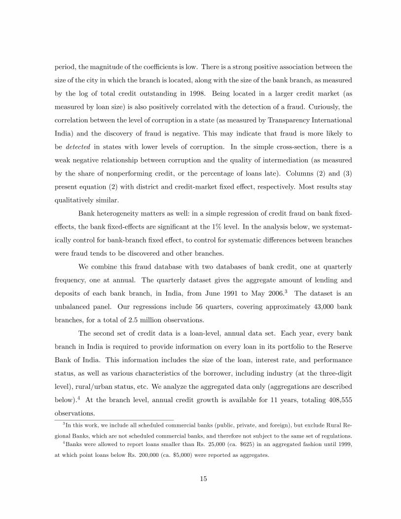
period, the magnitude of the coe¢ cients is low. There is a strong positive association between the

size of the city in which the branch is located, along with the size of the bank branch, as measured

by the log of total credit outstanding in 1998. Being located in a larger credit market (as

measured by loan size) is also positively correlated with the detection of a fraud. Curiously, the

correlation between the level of corruption in a state (as measured by Transparency International

India) and the discovery of fraud is negative. This may indicate that fraud is more likely to

be detected in states with lower levels of corruption. In the simple cross-section, there is a

weak negative relationship between corruption and the quality of intermediation (as measured

by the share of nonperforming credit, or the percentage of loans late). Columns (2) and (3)

present equation (2) with district and credit-market �xed e¤ect, respectively. Most results stay

qualitatively similar.

Bank heterogeneity matters as well: in a simple regression of credit fraud on bank �xed-

e¤ects, the bank �xed-e¤ects are signi�cant at the 1% level. In the analysis below, we systemat-

ically control for bank-branch �xed e¤ect, to control for systematic di¤erences between branches

were fraud tends to be discovered and other branches.

We combine this fraud database with two databases of bank credit, one at quarterly

frequency, one at annual. The quarterly dataset gives the aggregate amount of lending and

deposits of each bank branch, in India, from June 1991 to May 2006.3 The dataset is an

unbalanced panel. Our regressions include 56 quarters, covering approximately 43,000 bank

branches, for a total of 2.5 million observations.

The second set of credit data is a loan-level, annual data set. Each year, every bank

branch in India is required to provide information on every loan in its portfolio to the Reserve

Bank of India. This information includes the size of the loan, interest rate, and performance

status, as well as various characteristics of the borrower, including industry (at the three-digit

level), rural/urban status, etc. We analyze the aggregated data only (aggregations are described

below).4 At the branch level, annual credit growth is available for 11 years, totaling 408,555

observations.3 In this work, we include all scheduled commercial banks (public, private, and foreign), but exclude Rural Re-

gional Banks, which are not scheduled commercial banks, and therefore not subject to the same set of regulations.4Banks were allowed to report loans smaller than Rs. 25,000 (ca. $625) in an aggregated fashion until 1999,

at which point loans below Rs. 200,000 (ca. $5,000) were reported as aggregates.

15

The two datasets are complementary: the higher frequency of the quarterly dataset

allows for better measurement: frauds are of course discovered throughout the year, and with

quarterly data, we are better able to pin down the short- and medium-term e¤ects of the

discovery of fraud. The quarterly data also provide a longer time series, 15 years. To delve deeper

into the e¤ects of vigilance activity, we use the annual dataset, which includes information on

the repayment status of loans and the industries to which banks lend.

Both the quarterly and annual datasets identify bank, branch, credit market, district,

and date. Approximately 10% of the credit data is missing: this occurs when a bank does not

report required information.

Taken together, this data form, to our knowledge, one of the richest data sets on fraud

in the banking sector, and its implication for lending. Due to the highly con�dential nature of

the data, all data analysis was performed at the Reserve Bank of India, either by one of the

researchers on site, or using codes that was provided by us.

5 Fraud Discovery and Punishment

5.1 The Impact of the Discovery of a Fraud on Vigilance Activity

To test the main predictions of the model, our empirical strategy will be to exploit the increase

in the probability of being investigated or punished for default after a fraud has occurred in a

particular branch. In the model, the probability that the regime of high inspection continues

into the next period is an important parameter: it makes sense for a loan o¢ cer to bail out a

�rm during a �high inspection regime" if she expects that the probability of inspection will be

lower in the future. Thus, this section focuses on how the probability of fraud detection evolves

over time following the discovery of a fraud in one particular branch.

As we already noted, the probability of detection is very low: the probability of any given

branch reporting a suspected fraud is only 1.2% over the entire 15-year period of our data. In

any given year, the unconditional probability of vigilance activity is 8 basis points. However,

there is very large serial correlation in inspections. To understand how an investigation a¤ects

the subsequent probability of a detection ocurring, we estimate the following model:

16

Db;t = �+5Xn=1

Db;t�n + "b (4)

where Db;t is a dummy variable taking the value of 1 if the branch reports a suspected fraud in

year t, and 0 otherwise. Regression results are displayed in Panel B, for a lag structure including

1-5 lags. Two results stand out: �rst, if a fraud was detected in a given year, the probability

of detection in the subsequent year, relative to a branch in which no fraud was detected, is

substantially increased. The coe¢ cient on Db;t�1 is .023, indicating an increased probability of

2.3 percentage points. Relative to the baseline probability of 8 basis points, this represents a

an increase by a factor of 29 times. Second, the probability of heightened vigilance drops by

half the following year, and remains at that level after two years. After three years, however,

the probability of detection is very low, indistinguishable from the probability of detection in a

branch with no history of fraud detection.

Part of the increase in the probability of detection certainly comes from the fact that

the same set of people are likely to have committed more than one fraud. The investigation of

one fraud reveals all the older ones. In fact, this is probably what prompts the vigilance team to

investigate this branch thoroughly. But as they do so, it is also likely that they investigate the

lending activities of others in the bank. Thus, we take this data to suggest that fraud discovery

in a bank creates a large increase in the probability of subsequent investigation, which persist

for about two years. In the next section, we will investigate how lending decisions respond to

this temporary increase in vigilance activity.

5.2 The Shape of the Penalty Function

The shape of the penalty function is an important parameter in the model. With a F (:) su¢ -

ciently convex, ever-greening could be entirely avoided.

While it is di¢ cult to get data that precisely pins down the shape of the penalty function,

discussions with bankers and media suggest that it is increasing, but rather �at: the standard

penalties for having been found guilty of frauds is a reduction in pay, transfers, and in the

worst case, dismissal. This holds true in our dataset; visual inspection (a categorization was not

available) suggested pay reduction as the primary mechanism.

17

Further evidence that the penalty function is �at comes from an exercise conducted

by the Central Vigilance Commission. In order to stigmatize corruption, the CVC decided to

publish on its website the names, and penalties, of senior-level o¢ cers who had been found

guilty of corruption. While the speci�cs of the fraud committed were not disclosed, because the

bankers worked at the highest level, the frauds likely involved very large sums. Of the 76 bank

o¢ cials for whom data was made public, the distribution of penalties was:

Outcome Frequency

Criminal Charges Filed 1

Censured 2

Obligatory Retirement 4

Dismissed 21

Pay Reduction 46This, in our mind, provides strong evidence that the penalty for fraud is not commen-

surate with the amounts involved, let alone convex: a large part of the cost seems to be the

investigation itself, which appears to be quite traumatic for low-level loan o¢ cers. But the pun-

ishments, even for large frauds, mainly involved a pay reduction. This of course begs the question

of why the penalty function is not made more convex: this could be achieved by not prosecuting

a loan o¢ cer until several of their loans appear to have a suspected fraud, and by handing

out much more severe punishment once someone is actually investigated and proven guilty. It

may be particularly tempting for bankers accused of large fraud to bribe the CVC investigators.

Thus, the need to maintain an arm�s length relationship between the bank administration and

the CVC may be the reason why the penalty function cannot be convex.

6 Empirical Tests of the Model

6.1 Lending Decisions

We now turn to testing a central prediction of our model: does vigilance activity reduce lending

activity? To investigate this question, we treat the discovery of a fraud in a branch as an �event�

and study how lending in this bank changes after the discovery of the fraud, compared to other

una¤ected branches.

18

6.1.1 Branch-Level E¤ects

We use an event-study (di¤erence-in-di¤erence) methodology to measure the impact of vigilance

activity on lending. This strategy compares how lending evolves in branches that are a¤ected

by fraud investigations, to other similar branches that are not.

The base speci�cation uses quarterly lending data, at the branch-level. Denote yobct as

the change in log credit at bank branch o¢ ce o, belonging to bank b, in credit market c, at time

t: The estimated equation is thus:

yobct = �o +

8Xk=�8

�kDo;t;k + ��9Do;t;�9 + t + "obct; (5)

where yobct is log credit growth, de�ned as log(creditobc;t=creditobc;t�1).5 Do;t;k indicate

the detection of the fraudulent act. Thus Do;t;0 is set to one if a fraud occurs in branch o¢ ce o

in quarter t, and zero otherwise, while Do;t;�3 is set to 1 if a fraud will occur in branch o¢ ce o

at time t+3. Do;t;�9 is dummy variable indicating a fraud was committed nine or more quarters

previous to quarter t in branch o¢ ce o. ao and t denote branch and quarter �xed-e¤ects,

respectively, which we include in the preferred speci�cation.

Table 4 reports results from the baseline speci�cation, for the sample of frauds coded as

�extension of credit for illegal grati�cation�or �other, credit related.�Under the null hypothesis

that vigilance activity does not a¤ect lending, the coe¢ cients � should be zero.6 Column (1)

reports results from Equation (5) without branch or time �xed e¤ects. Column (2) adds quarter

�xed e¤ects ( t); column (3) adds branch �xed e¤ects (a0); and column (4) presents the results

with quarter and branch o¢ ce �xed e¤ects. Column (4) is the preferred speci�cation, as the

branch �xed e¤ects control for all unobserved time-invariant heterogeneity, while the quarter

�xed e¤ects control for aggregate changes in credit at the national level.

This regression is perhaps best understood graphically: Figure 1 displays the coe¢ cients

from the preferred speci�cation for each event time (eight quarters prior to an event, seven

quarters prior, etc...) The blue line gives the point estimate, while the yellow lines give the 95-

5We use log credit growth, rather than log credit, because credit is highly serially correlated, and because

credit growth may be more relevant than the stock of credit.6The average size of a fraudulent loan is a quite small relative to the branch portfolio, so there is no mechanical

relationship between discovery of fraud and the amount of lending.

19

percent con�dence interval. The line therefore traces how credit evolves prior to the discovery

of a fraud, and following a fraud.

A clear pattern emerges. The corrupt loan is discovered at time zero. Prior to this

discovery, credit typically evolves at a rate no di¤erent than at other branches, with the exception

of �six months prior�and �three months prior,�when the growth rate is above average (this may

have been what prompted the investigation, or this may be a symptom of fraudulent activity).

Following the discovery of fraud, credit growth drops precipitously, relative to other branches: by

1.36 percent relative to branches in which a fraud is not discovered in the quarter of discovery

(column (4)). In the subsequent quarter, credit growth is 3.73 log points below una¤ected

branches. This is a very large e¤ect: the average growth rate in credit is 3.5% per quarter,

meaning that following an investigation, the credit growth is stagnant. Credit continues to grow

at a slower pace following the discovery of the fraud, with a cumulative e¤ect of nearly twenty

percent less credit lent by an a¤ected branch after two years. The �nal coe¢ cient, Do;t�9, is

negative and signi�cant, suggesting that credit continues to decline (relative to other branches)

even two years after the discovery of the fraud.

Even though our dependent variable is change in log credit, speci�cation 5 is likely

to su¤er from serial correlation. Running a regression with branch and quarter �xed e¤ects,

and 2.5 million observations, correcting for non-independence of error terms in SAS taxes the

available computer facility, so the majority of the regressions presented in this paper are currently

presented with unadjusted standard errors.7 However, in an appendix table we present the

baseline speci�cation, with corrected and uncorrected standard errors. Correcting the standard

errors has little e¤ect on the measured precision of the estimates: only one �pre�coe¢ cient is

statistically distinguishable from zero, the �post� coe¢ cients remain negative and similar in

size, though three of the eight are not statistically distinguishable from zero. The t-statistic on

the e¤ect one quarter after discovery of the fraud remains very high, approximately 5.5.

Table 5 estimates equation (5) with a longer series of post-event dummies, tracing the

e¤ect up to two years later. The results for the branch-level identi�cation are presented in

column (1). Including sixteen post dummies reduces the sample size by two years of fraud

discovery, but provides a longer picture of the e¤ect. The results are nearly identical: the e¤ect

7This is due to time constraints. Subsequent versions of this paper will have corrected standard errors.

20

of discovery of fraud is negative and signi�cant for the �rst eleven quarters following discovery,

with a cumulative e¤ect of 21 percent less credit.

What explains the persistence of the e¤ect on lending, despite the fact that the increase in

the vigilance activity in the branch stops relatively quickly? Our model predicts some temporal

propagation of shocks. First, mechanically, the volume of loans will be reduced as the vigilance

o¢ cer discovers evergreening. Second, as loan o¢ cers fear increased scrutiny, they reduce the

size of loans to new �rms. Because the informativeness of a failure is increasing in the size of

the loan, loan o¢ cers on average learn less about new �rms in the vigilance period; then, even

when the monitoring threat has reduced, the optimal loan size is smaller. However, �rms in

our model live only two periods, and the model cannot explain as much persistence. In reality,

�rms leave longer than two periods, and thus the e¤ect may persist longer. The �rms who were

kept alive by successive evergreening, and who were cut from the portfolio during the vigilance

period, may in particular have otherwise continued to receive credit for a very long time. It is

therefore di¢ cult to conclude whether this persistence is a good thing or a bad thing. Another

reason for the stickiness of the e¤ect may be because the investigation remains salient in the

minds of loan o¢ cers, even as the probability of investigation decreases dramatically.

6.1.2 Spillover E¤ects of Vigilance Activity

In this section, we investigate whether the investigation has spillover e¤ects to other branches

in the same area: do other branches of the same banks in the town also stop lending when a

particular branch is investigated following the discovery of a fraud? How about other banks in

the same town?

To interpret these results, we �rst need to investigate whether discovery of fraud in a

branch increases the probability a fraud will be discovered in other branches of the same bank in

the next year, and other branches in the same town. We investigate this question by augmenting

equation (4) with a dummy for whether a fraud was discovered in another branch of the same

bank in the same town in the previous year, and a dummy for whether a fraud was discovered in

another branch in the town in the previous year. Both e¤ects are signi�cant, although they are

smaller than the direct e¤ect: when a branch of the same bank in the same town, the probability

of inspection increases by 0.9 percentage point (about half the size of the direct e¤ect). The

21

increase is only 0.2 percentage point if another branch of the same branch, but in a di¤erent

town, was investigated, although the increase number remains signi�cant.

Since there was an e¤ect on the probability of inspection, we may expect an e¤ect on

lending on those branches as well.

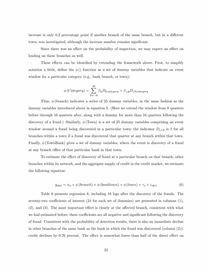
These e¤ects can be identi�ed by extending the framework above. First, to simplify

notation a little, de�ne the � () function as a set of dummy variables that indicate an event

window for a particular category (e.g., bank branch, or town):

� (Category) =

16Xk=�8

�kDk;category + ��9D�9;category

Thus, � (branch) indicates a series of 25 dummy variables, in the same fashion as the

dummy variables introduced above in equation 5. (Here we extend the window from 8 quarters

before through 16 quarters after, along with a dummy for more than 16 quarters following the

discovery of a fraud.) Similarly, � (Town) is a set of 25 dummy variables comprising an event

window around a fraud being discovered in a particular town: the indicator Dc;t;0 is 1 for all

branches within a town if a fraud was discovered that quarter at any branch within that town.

Finally, � (TownBank) gives a set of dummy variables, where the event is discovery of a fraud

at any branch o¢ ce of that particular bank in that town.

To estimate the e¤ect of discovery of fraud at a particular branch on that branch, other

branches within its network, and the aggregate supply of credit in the credit market, we estimate

the following equation:

yobct = �o + � (branch) + � (banktown) + � (town) + t + "obct (6)

Table 6 presents regression 6, including 16 lags after the discovery of the frauds. The

seventy-two coe¢ cients of interest (24 for each set of dummies) are presented in columns (1),

(2), and (3). The most important e¤ect is clearly at the a¤ected branch, consistent with what

we had estimated before: these coe¢ cients are all negative and signi�cant following the discovery

of fraud. Consistent with the probability of detection results, there is also an immediate decline

in other branches of the same bank as the bank in which the fraud was discovered (column (2)):

credit declines by 0.76 percent. The e¤ect is somewhat lower than half of the direct e¤ect on

22

the bank branch. This e¤ect is short-lived, however. There does not appear to be a marked

increase in lending by other branches in response to the reduced supply of credit. This again is

consistent with the much lower impact of lending on those branches. Interestingly, we do not

see an increase in lending by the other branches, which could have happen if all the clients of

the branch that stopped lending moved to other banks.

These results are of independent interest. They also provide some reassurance that the

results are indeed due to the causal e¤ect of the increase in the probability being investigation

for fraud, since, from the point of view of other branches in the same town, the discovery of a

fraud in another branch is an exogenous event.

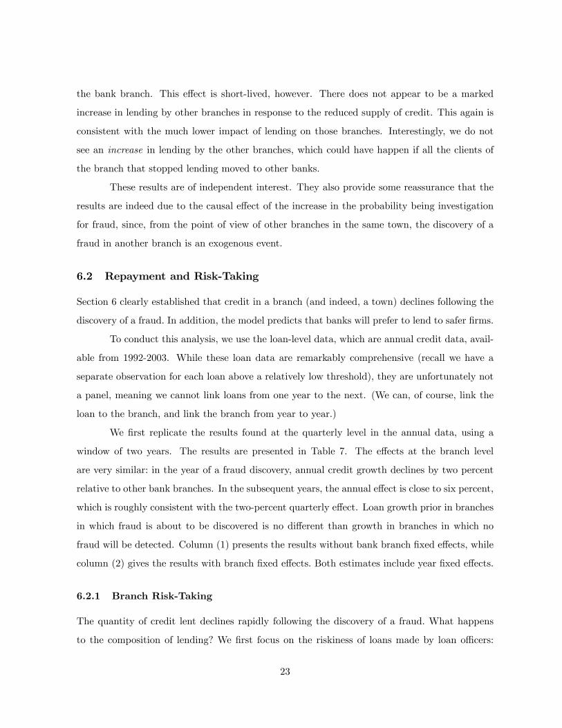
6.2 Repayment and Risk-Taking

Section 6 clearly established that credit in a branch (and indeed, a town) declines following the

discovery of a fraud. In addition, the model predicts that banks will prefer to lend to safer �rms.

To conduct this analysis, we use the loan-level data, which are annual credit data, avail-

able from 1992-2003. While these loan data are remarkably comprehensive (recall we have a

separate observation for each loan above a relatively low threshold), they are unfortunately not

a panel, meaning we cannot link loans from one year to the next. (We can, of course, link the

loan to the branch, and link the branch from year to year.)

We �rst replicate the results found at the quarterly level in the annual data, using a

window of two years. The results are presented in Table 7. The e¤ects at the branch level

are very similar: in the year of a fraud discovery, annual credit growth declines by two percent

relative to other bank branches. In the subsequent years, the annual e¤ect is close to six percent,

which is roughly consistent with the two-percent quarterly e¤ect. Loan growth prior in branches

in which fraud is about to be discovered is no di¤erent than growth in branches in which no

fraud will be detected. Column (1) presents the results without bank branch �xed e¤ects, while

column (2) gives the results with branch �xed e¤ects. Both estimates include year �xed e¤ects.

6.2.1 Branch Risk-Taking

The quantity of credit lent declines rapidly following the discovery of a fraud. What happens

to the composition of lending? We �rst focus on the riskiness of loans made by loan o¢ cers:

23

if lenders are afraid that a bad loan may land them in hot water, they may prefer to lend to

borrowers who are less likely to default. We do not observe the credit rating of the borrower (for

this time period, there is no formal credit rating institution, and this data set does not include

data on the credit-worthiness of the borrower). Instead, we exploit the fact that some industrial

sectors are riskier than others. We calculate how risky each industrial sector is, measuring the

percentage of loans in that sector that are late in repayment. This measure could vary from zero

to 100:

sharelatei = 100 �Value of Lending in Industry that is Non-Performing in 1992

Lending in Industry in 1992:

We then take the share of credit lent by each branch o to industry I, to come up with a

predicted portfolio riskiness :

branchriskot =X

i2Industries

Value of Branch lending to IndustryValue of all Branch Lending at time t

� sharelatei

Note that branchriskot is not determined by the share of loans late at branch o: rather, it

measures the share of loans with late repayment predicted by the industrial composition of

lending.

Table 8 reports how branchriskot varies following the discovery of an alleged fraud.

Column (2) presents equation (5) with branch and year �xed e¤ects. Two years prior to the

discovery of fraud, the measure of risk exposure is no di¤erent than branches in which a fraud

is not about to be discovered. One year prior to the fraud, the level of risk taking is elevated.

However, one year following the discovery of fraud, the riskiness of the loan portfolio drops

substantially, with branchriskot falling approximately eight percentage points. The standard

deviation of branchriskot is approximately seven percentage points, so this represents a signi�cant

drop.

This �nding is consistent with the model, which predicts that lending to old, successful

�rms will be increasing in the posterior probability that the �rm the good type.

24

6.2.2 Loan Repayment

Credit drops substantially following discovery of a fraud, as does the risk-taking behavior of

bank branches. What happens to the quality of loans made by an a¤ected branch?

Because we do not observe a panel of loans, we cannot di¤erentiate loans made prior to

discovery of fraud from loans made after discovery. Instead, we focus on the growth in total

credit, and the growth in bad credit.

The e¤ect on aggregate credit is presented in columns (1) and (2) of Table 9. Columns

(2) and (4) include branch �xed e¤ects. Column (3) shows that the total amount of credit

marked as late is much higher in the year in which the fraud is discovered, drops in the following

year, and again increases slightly above the steady state in the following year. The increase in

the year of the discovery is probably mechanical: as the CVC team investigates the bank, they

identify a number of loans that are to be written o¤. The reduction of default in year t + 1,

followed by an increase the following year, is consistent with the ever-greening predicted by the

model: in year t + 1, the loan o¢ cer ever-greens to avoid default, and this tends to reduced

default (even though that coe¢ cient is not signi�cant). However, some of the �rms that were

arti�cially supported then fail by the following year, which leads to a sharp increase in default

by year t+2, before things go back to normal in year t+3. It is interesting that this time series

pattern �ts the model so closely.

6.3 An Attempt At Reform

On January 1, 1999, the Central Vigilance Commission, in response to criticism mentioned

above, introduced a special chapter of the Vigilance Manual. The goal of this chapter was to

clarify the standards and procedures of investigation of employees of public sector banks. This

suggests a natural experiment: if the manual changed the incentives faced by loan o¢ cers, the

e¤ects of investigation should change.

To test this, we estimate equation (5) using two sets of D variables: one set for the

period before January 1, 1999, and one set for the period after 1999. Results are presented

in Table 10. The results suggest that the new vigilance chapter did not change the e¤ect of

a vigilance investigation: the � coe¢ cients are very similar in the pre-and post-reform period.

Panel B gives the cumulative e¤ect of three years following the discovery of the fraud (the value

25

�0+�1+�2+��3): The cumulative e¤ect prior to the reform is -8.15, which is indistinguishable

from the cumulative e¤ect following the reform, of -7.64.

The ine¢ cacy of the manual was predicted in early 2002 by a Public Sector Bank Manager

in the newspaper �The Hindu:�

A deeper examination would clearly show that a separate manual is unlikely to

improve the matter of oppressive levels of accountability in PSBs. To recall a similar

Governmental supervision, in 1992 when the country was almost on the verge of

insolvency and industrial growth was at low levels, one of the constraints to growth

was identi�ed as controls on creation of new industrial capacity. The then Finance

Minister did not substitute one licensing policy by another, but abolished licensing

requirements for all but a handful of industrial sectors. The results of this bold

action are there for all to see.8

7 Conclusion

This paper derives and tests a model of bank lending behavior, in the face of outside supervision.

We then test this model using an unusual data set from India, which combines data on almost

all the credit frauds detected over two decades and the universe of loans over a long period.

The data largely support the main predictions of the model: lending declines following vigilance

activity, bankers shift to less risky industries, and defaults follow a very speci�c pattern: after

the initial increase due to the vigilance activity, they decline to levels below the �normal" level

of default, only to increase again to high levels in the following year.

These �ndings are con�rmed using two independent datasets on vigilance activity, in

quarterly, and annual fraud data. The most precise estimate comes from quarterly branch loan

data: immediately following an investigation, lending falls 4% relative to non-a¤ected branches,

and this e¤ect is quite persistent, lasting over two years. The e¤ect occurs primarily at the

a¤ected branch, but spills over to other branches of the same bank in the same credit market

(which appears to be also a¤ected by heightened vigilance). Other bank branches in the market

did not increase lending to �replace� the missing credit. There is no systematic increase (or

8R. Viswanathan, The Hindu, Jan 12, 2002

26

decrease) in credit prior to discovery of a fraud, implying that the observed e¤ects may have a

causal interpretation. Thus, in a very real sense, the bank o¢ cers are correct: fear of prosecution

causes lending o¢ cers to act substantially more cautiously than their peers, who are not a¤ected

by recent discovery of fraud.

Determining whether these e¤ects are e¢ cient or ine¢ cient is more di¢ cult. We present

suggestive evidence that vigilance activity is linked to �under-lending.�Given that prior research

provides evidence of credit constraints in precisely this context, vigilance activity may indeed

be ine¢ cient. First, the fact that vigilance activity a¤ects aggregate lending at the bank level,

is hard to reconcile a bank-wide slowdown in credit following the charge of a single (albeit

prominent) individual. Second, the e¤ect is found in other branches belonging to the same bank

in the same town. Third, the size of the credit declines are much larger than the amount of

money involved in the fraud, and are very persistent. Finally, we see that the lending strategy

taken by the a¤ected branch changes substantially. Rather than �root out�a corrupt o¢ cer and

continue to lend to the optimal mix of borrowers, bank branches a¤ected by a vigilance activity

shift lending towards safer industries.

27

8 References

Banerjee, Abhijit, and Esther Du�o, 2004. �Do Firms Want to Borrow More? Testing Credit

Constraints Using a Directed Lending Program,�working paper, MIT.

Banerjee, Abhijit, and Esther Du�o, 2008. �Growth Theory Through the Lens of Development

Economics,�Elsevier Handbook of Macroeconomics.

Beck, Thorsten, Asli Demirguc-Kunt, and Ross Levine, �Bank Supervision and Corruption in

Lending,�forthcoming, Journal of Monetary Economics.

Berger, Allen, and Rebecca Demsetz, and Phillip Strahan, 1997. �Diversi�cation, Size, and

Risk at Bank Holding Companies,�Journal of Money, Credit, and Banking, vol 29.

Central Vigilance Commission 2000, �Cases Referred to the Central Vigilance Commission by

Public Sector Banks: A Critical Analysis,�Central Vigilance Commission, Delhi.

Central Vigilance Commission 2001, �Special Chapter on Vigilance Management in Public

Sector Banks vis-à-vis The Role and Functions of the CVC�Central Vigilance Commission,

Delhi.

Cole (2008) �Fixing Market Failures or Fixing Elections: Agricultural Credit in India,�forth-

coming, American Economic Journals: Applied Economics.

Dinc, Serdar (2006). �Monitoring the Monitors: The Corporate Governance in Japanese Banks

and Their Real Estate Lending in the 1980s,�Journal of Business, 79(6): 3057-3081.

Galor, O. and J. Zeira (1993). "Income Distribution and Macroeconomics." Review of Economic

Studies 60(1): 35-52.

Gupta, Manash, and Sarbajit Chaudhuri, �Formal Credit, Corruption and the Informal Credit

Market in Agriculture: a Theoretical Analysis,�Economica (64):331-43.

Khwaja, Asim and Atif Mian (2005). �Do Lenders Favor Politically Connected Firms? Rent

Provision in an Emerging Financial Market�The Quarterly Journal of Economics, 120(4):

1371-1411.

28

Khwaja, Asim, and Atif Mian (2007). �Tracing the Impact of Bank Liquidity Shocks: Evidence

from an Emerging Market,�forthcoming, American Economic Review.

de Mel, Suresh, David McKenzie, and Christopher Woodru¤, 2006. �Returns to Capital in

Microenterprises: Evidence from a Field Experiment,�Working paper, World Bank.

Hertzberg, Andrew, Jose Liberti, and Daniel Paravasini (2007). �Information and Incentives

Inside the Firm: Evidence from Loan O¢ cer Rotation,�manuscript, Columbia University.

Mookherjee, Dilip (2006), �Decentralization, Hierarchies, and Incentives: A Mechanism Design

Perspective.�

Rajan, Raghu (2004). �Why Bank Credit Policies Fluctuate: A Theory and Some Evidence,�

Quarterly Journal of Economics, Vol. 109, No. 2: 399-441.

Stein, Jeremy (2002). "Information Production and Capital Allocation: Decentralized versus

Hierarchical Firms," Journal of Finnace, LVII(8): 1891-1921.

Tannan, M, 2001, �Banking Law and Practice in India,�India Law House: New Delhi.

29

Figure 1: Effect of Vigilance Activity

-5

-4

-3

-2

-1

0

1

2

3

4

-8 -7 -6 -5 -4 -3 -2 -1 0 1 2 4 5 6 7 8 9+

Time Relative to Event

Log

Cha

nge

Cre

dit (

Perc

ent)

Point-2SD+2SD

Table 1: Summary Statistics for Bank-Level Analysis

Panel A: Credit Data

January 1992 (Real 1984 Rs.)Mean Median

Loans, Cash Credit, and Overdrafts 156,943 74,942(214,331)

Log(Loans, Cash Credits and overdrafts) 16.98 16.65(0.830)

January 2000 (Real 1984 Rs.)Mean Median

Loans, Cash Credit, and Overdrafts 296,060 166,431(382,644)

Log(Loans, Cash Credits and overdrafts) 12.24 12.02(0.753)

Sample Size

Number of Public Sector Banks 27Number of Months (Jan. 1992 - May 2001) 111Number of Observations 2997

Note: Standard deviations are given in parenthesesCredit data from the Reserve Bank of India

Panel B: Central Vigilance Committee Data

1993 1994 1995 1996 1997 1998 1999 2000Advice 1 7 4 7 13 15 9 12Order 1 4 3 6 10 10 13 4Total 2 11 7 13 23 25 22 16

CVC Advice CVC OrderAction

Prosecution 12.2Charge Sheet Filed 2.2Information Awaited 14.4Dismissal of Employee 16.7 18.9Compulsory Retirement 5.6 4.4"Major Penalty" 50.0

Pay ReducationReduction in Pay 1 Grade 2.2 22.2Reduction in Pay 2 Grades 7.8 13.3Reduction in Pay 3 Grades 4.4Reduction in Pay 4 Grades 2.2 5.6Reduction in Pay 5 Grades 1.1

Other 3.3 13.3

Yearwise Distribution of Cases

Distribution of Content of CVC Advice and Orders (Percentage)

indexIndicator for Vigilance Activity Deposits Securities Other Assets

(1) (2) (3) (5) (6)Indicators for Vigilance Activity

Twelve Months Prior -0.02 -0.02 0.00 -0.07(0.01) (0.02) (0.02) (0.22)

Nine Months Prior -0.02 -0.02 0.00 -0.28(0.01) (0.02) (0.02) (0.22)

Six Months Prior -0.02 * -0.03 0.00 -0.09(0.01) (0.02) (0.02) (0.22)

Three Months Prior -0.03 ** -0.02 -0.01 -0.17(0.01) (0.02) (0.02) (0.22)

Contemporaneous -0.04 *** -0.03 ** -0.02 -0.01 0.15(0.01) (0.01) (0.02) (0.02) (0.22)

Three Months Following -0.04 *** -0.03 ** -0.03 -0.02 -0.20(0.01) (0.01) (0.02) (0.02) (0.22)

Six Months Following -0.03 ** -0.03 ** -0.02 -0.01 0.40 *(0.01) (0.01) (0.02) (0.02) (0.23)

Nine Months Following -0.03 * -0.02 -0.03 0.00 0.21(0.01) (0.01) (0.02) (0.02) (0.23)

Twelve Months Following -0.04 ** -0.02 -0.02 -0.01 0.75 ***(0.01) (0.01) (0.02) (0.02) (0.22)

Eighteen Months Following -0.03 * -0.03 -0.03 * 0.37(0.01) (0.02) (0.02) (0.23)

Twenty-Four Months Following -0.02 -0.04 -0.01 0.33(0.02) (0.02) (0.02) (0.25)

Month Fixed Effects Y Y Y Y YBank Fixed Effects Y Y Y Y Y

Dependent Variable: Log CreditNotes

Table 2: The Effect of Vigilance Activity on Bank Behavior

Columns (1)-(3) present panel regressions of log credit extended by twenty-seven public sector banks, over a period of 111 months, giving 2997 observations. Standard errors (robust to heteroskedasticity and serial correlation) are reported in parentheses. Columns (5)-(7) present similar regressions for other balance sheet items.2 - The independent variable of interest is a dummy variable indicating whether the CVC had charged or punished an officer of a particular bank in a particular month.3 - Column (1) displays the results of regressing log credit on bank and year fixed effects, as well as a dummy for whether there was vigilance activity in a particular bank that month.4 - Columns (2) and (3) examine how the effect persists over time. In column (2), log credit is regressed on dummies for whether there was vigilance activity in a bank for the previous one, two, three, …, twelve months. For consiseness, only the coefficients for contemporaneous, three, six, and twelve months are reported. Column three traces the effects over the past 48 months: again, only coefficients for the contemporaneous effect, and months 3, 6, 12, 18, 24, 36, and 48 are reported.

Credit

Panel A: FraudGeneral Frauds Data Overview

Number of ObservationsFraud Type Frequency"Extension of Credit for Illegal Gratification" 354"Other" 1378Total 1732

Panel B: Areas of Bank Operation in Which Frauds OccurCredit Other

Deposits 0 36Credit (i) Savings 6 77

her Other 21 42Total 4 13

Panel C: Time to Discovery of FraudsNumber of Days Credit OtherAverage 559 41525th Percentile 188 28Median 396 18375th Percentile 745 534

Panel D: Size of FraudAverage 114 27025th Percentile 4 1Median 20 375th Percentile 70 14

Panel E: Decade of Fraud1950-1979 12 231980s 58 1111990s 148 3992000s 132 849

Notes: This table provides a basic overview of the data on frauds available for the study.All frauds involve loan officers at the local (branch) level.

Table 3: Summary Statistics

Classification

Classification

index

Panel B: Credit Summary StatisticsN Mean Std. Dev # of Frauds

Quarterly Jan '80 - March 2006Change in Log Credit 2,493,537 3.50% 2.78% 1400

Annual 1992 - 2005 But relaly only goes to 2003 b/c of lags?Change in Log Credit 405,227 12.45% 1200Change in Log (Late Credit) 245,774 -3.04% 1200Share of Loans Late (Value-Weighted) 365,909 15% 1200

Distribution of Loan Sizes 1992Average $598Minimum $025th Percentile $61Median $10575th Percentile $170Max >$50m

Panel C: Detailed Fraud Breakdown

Types of Fraud Total 1980s 1990s 2000s 1980s 1990s 2000sExtension of Credit 323 46 126 151 57 143 123 for Illegal GratificationOther 1064 79 272 713 103 356 605 Of which, related to credit 539 45 86 408 60 132 347Total 1387 125 398 864 160 499 728

Share of Frauds in Time Period in Government Banks

Extension of Credit 0.90 0.89 0.87 0.92 0.89 0.87 0.93 for Illegal GratificationCredit-Related Other 0.80 0.91 0.80 0.78 0.90 0.81 0.78

Size of Fraud (Occurrence) Overall 1980s 1990s 2000sAverage Rupees (000) 506.4 98.2 210.2 701.8Average $(000) (roughly) 14.5 2.8 6.0 20.1

.Minimum $ 0 0 0 0 .25th Percentile $ 94 102 112 90 .Median $ 312 357 468 265 .75th Percentile $ 1,314 1,247 1,748 1,104 .Max $ 13,868,114 112,414 489,494 13,868,114 .

. .

. .

Detection Occurrence

Table 3, Continued

Panel A: Univariate Regressions(1) (2) (3) (4) (5) (6) (7) (8) (9)

Public Bank -0.03 -1.31 *** 1.10 ***(0.13) (0.22) (0.20)

More Urban Location 0.45 *** 0.28 *** 0.49 *** 0.30 *** 1.05 *** 0.03(0.02) (0.03) (0.02) (0.03) (0.09) (0.15)

Log Branch Size 0.91 *** 0.58 *** 0.72 *** 0.86 *** 0.61 *** 0.75 *** 1.37 *** 0.17 0.33(0.04) (0.04) (0.07) (0.04) (0.04) (0.08) (0.15) (0.18) (0.31)

Number of Branches in Market 0.01 *** 0.01 *** 0.01 *** 0.01 *** 0.02 *** 0.00(0.00) (0.00) (0.00) (0.00) (0.00) (0.01)

Log Credit Market Size 0.40 *** 0.28 *** 0.41 *** 0.29 *** 1.37 *** 0.02(0.01) (0.03) (0.02) (0.03) (0.10) (0.23)

More Corrupt State -58.15 *** -52.05 *** -106.65 **(9.65) (11.22) (42.08)

Share of Credit Nonperforming -0.49 * 0.34 0.72 -0.11 0.51 * 1.11 ** -3.40 2.25 0.37(0.27) (0.30) (0.55) (0.27) (0.29) (0.56) (2.12) (2.25) (4.48)

Share of Loans Nonperforming -0.02 0.28 0.60 0.29 0.45 * 0.95 * -1.89 1.28 1.47(0.25) (0.27) (0.48) (0.25) (0.27) (0.49) (1.66) (1.74) (3.17)

FE None District Credit Market None District Credit Market None District Credit Market

Panel B: Conditional Correlations Conditional Correlations

(1) (2) (3) (4) (5) (6) (7) (8) (9)Public Bank -0.96 *** -1.36 *** -1.34 ***

(0.25) (0.26) (0.35)More Urban Location

Log Branch Size 0.35 *** 0.51 *** 0.70 *** 0.39 *** 0.53 *** 0.75 *** 0.29 0.29 0.34 ***(0.05) (0.05) (0.08) (0.05) (0.06) (0.08) (0.24) (0.26) (0.32)

Log Credit Market Size 0.37 *** 0.10 *** 0.31 *** 0.11 *** 1.34 *** -0.01(0.02) (0.03) (0.02) (0.03) (0.12) (0.23)

More Corrupt State -40.36 *** -30.55 ** -188.82 ***(12.06) (12.06) (58.90)

Share of Credit Nonperforming 0.64 ** 0.54 * 0.82 0.60 ** 0.48 0.75 -2.13 1.11 0.08(0.31) (0.33) (0.58) (0.30) (0.32) (0.59) (3.21) (3.58) (4.80)

Notes: Each cell represents a regression. The unit of observation is a bank branch (there are 49,484 branches, of which 44,547 are public, 4,700 are private, and 237 are foreign).The dependent variable is equal to 100 if a fraud was discovered at that branch between 1980 and 2005. The dataset identifies 898 frauds.

Table 4: Where are Frauds Detected?All Banks Public Banks Private Banks

All Banks Public Banks Private Banks

index

Time Window Branch-Level Town-level District-level(1) (2) (3)

Quarter - 8 0.62 -0.18 -0.2 **(0.48) (0.12) (0.08)

Quarter - 7 -0.06 0.01 0.03(0.47) (0.12) (0.08)

Quarter - 6 0.48 0.38 *** 0.15(0.47) (0.12) (0.08)

Quarter - 5 1.02 ** -0.02 -0.01(0.46) (0.12) (0.08)

Quarter - 4 0.6 0.1 0.12(0.46) (0.12) (0.08)

Quarter - 3 1.48 *** 0.06 0.14(0.46) (0.12) (0.08)

Quarter - 2 1.4 *** -0.42 *** -0.12(0.45) (0.12) (0.08)

Quarter - 1 1.3 *** -0.78 *** -0.24 ***(0.45) (0.12) (0.08)

Fraud Occurs 2.49 *** -0.23 ** -0.05(0.45) (0.11) (0.08)

Quarter + 1 1.11 ** -0.04 0.06(0.45) (0.12) (0.08)

Quarter + 2 0.21 -0.6 *** -0.22 **(0.45) (0.12) (0.09)

Quarter + 3 -0.36 -0.64 *** -0.18 **(0.45) (0.13) (0.09)

Quarter + 4 -1.43 *** -0.36 *** -0.2 **(0.46) (0.13) (0.09)

Quarter + 5 -0.88 -0.56 *** -0.18 **(0.46) (0.13) (0.09)

Quarter + 6 -1.38 *** -0.96 *** -0.4 ***(0.47) (0.13) (0.09)

Quarter + 7 -0.92 -0.36 *** -0.36 ***(0.47) (0.14) (0.09)

Quarter + 8 -1.51 *** -0.53 *** -0.12(0.48) (0.14) (0.09)

Nine Quarters and Beyond -1.66 *** -0.88 *** -0.37 ***(0.19) (0.06) (0.05)

0.42 0.42 0.42Fixed Effects Branch & Quarter Branch & Quarter Branch & QuarterN 2,493,609 2,493,537 2,493,537

Table 5: When Are Frauds Committed

All Frauds, Regressions at Branch Office LevelTime Window Log Change Log Change Log Change Log Change Log Change

(1) (2) (3) (4) (5)Quarter - 8 0.66 0.47 0.19 -0.06 -0.51

(0.58) (0.45) (0.59) (0.45) (0.11)Quarter - 7 0.97 * 1 ** 0.42 0.42 -0.13

(0.57) (0.44) (0.58) (0.45) (0.11)Quarter - 6 2.95 *** 2.61 *** 2.41 *** 2.06 *** 0.38

(0.57) (0.44) (0.58) (0.45) (0.11)Quarter - 5 1.73 *** 0.48 1.12 ** -0.12 -0.53

(0.56) (0.43) (0.57) (0.44) (0.11)Quarter - 4 1.72 *** 1.38 *** 1.11 * 0.8 * -0.09

(0.56) (0.43) (0.57) (0.44) (0.11)Quarter - 3 1.61 *** 1.83 *** 0.96 1.24 *** -0.12

(0.55) (0.43) (0.57) (0.44) (0.11)Quarter - 2 1.69 *** 0.74 * 1.05 * 0.17 -0.36

(0.55) (0.43) (0.56) (0.43) (0.11)Quarter - 1 0.21 0.41 -0.41 -0.14 -0.64

(0.55) (0.43) (0.57) (0.44) (0.11)Fraud Detected 0.04 -0.75 * -0.65 -1.36 *** -0.42

(0.56) (0.44) (0.58) (0.44) (0.12)Quarter + 1 -3.11 *** -3.13 *** -3.8 *** -3.73 *** -0.3

(0.57) (0.44) (0.58) (0.45) (0.12)Quarter + 2 -0.47 -1.48 *** -1.11 * -2.04 *** -0.41

(0.58) (0.45) (0.59) (0.46) (0.13)Quarter + 3 -1.96 *** -1.39 *** -2.6 *** -1.93 *** -0.57

(0.59) (0.45) (0.60) (0.46) (0.13)Quarter + 4 -0.31 -1.29 *** -0.93 -1.82 *** -0.61

(0.60) (0.47) (0.62) (0.47) (0.14)Quarter + 5 -2.05 *** -1.54 *** -2.65 *** -2.05 *** -0.25

(0.61) (0.48) (0.63) (0.48) (0.14)Quarter + 6 0.55 -1.47 *** 0.04 -1.9 *** -0.25

(0.63) (0.49) (0.65) (0.50) (0.14)Quarter + 7 -2.66 *** -1.73 *** -3.14 *** -2.12 *** -0.29

(0.64) (0.50) (0.66) (0.51) (0.14)Quarter + 8 -1.49 ** -1.55 *** -1.97 *** -1.95 *** -0.74

(0.66) (0.51) (0.68) (0.52) (0.14)Quarter > 8 -1.17 *** -1.36 *** -1.36 *** -1.59 *** -0.83

(0.13) (0.10) (0.27) (0.21) (0.06)N 2493542 2493542 2493542 2493542 2493537

Effect Identified for: Branch Branch Branch Branch Credit MarketFixed Effects None Quarter Branch Quarter & BranchTime Period 1990-2005 1990-2005 1990-2005 1990-2005

Notes:Each column represents a separate regression. The dependent variable, a measure of credit at the branch level, is indicated above the regression.Column (2)-(5) use change in log credit as the dependent variable.The regressions measure the effect of discovery of fraud on lending at the branch level.The approach is a difference-in-difference or "event study" methodology."Fraud Detected" is a dummy variable taking the value of 1 if a fraud was detected at a specific branch in a specific quarter.The "Quarter + N" dummy is equal to 1 at time t if a fraud was detected at that branch at time t-N.The "Quarter - N" dummy is equal to 1 at time t if a fraud was detected at that branch at time t+N.Columns 3 includes quarter fixed effects; Column 4 includes branch level fixed effects, and Column 5 includes branch and quarter fixed effects.Column 5 is the preferred specification.

Table 6: Effect of Discovery of Fraud on Lending

Clustered by Branch(1) (2)

Quarter - 8 -0.060 0.195(0.450) (0.584)

Quarter - 7 0.420 0.425(0.450) (0.571)

Quarter - 6 2.060 *** 2.412 ***(0.450) (0.570)

Quarter - 5 -0.120 1.124 *(0.440) (0.608)

Quarter - 4 0.800 * 1.116 *(0.440) (0.675)

Quarter - 3 1.240 *** 0.964(0.440) (0.662)

Quarter - 2 0.170 1.052(0.430) (0.661)

Quarter - 1 -0.140 -0.401(0.440) (0.675)

Fraud Detected -1.360 *** -0.639(0.440) (0.694)

Quarter + 1 -3.730 *** -3.785 ***(0.450) (0.684)

Quarter + 2 -2.040 *** -1.093(0.460) (0.698)

Quarter + 3 -1.930 *** -2.583 ***(0.460) (0.737)

Quarter + 4 -1.820 *** -0.913(0.470) (0.746)

Quarter + 5 -2.050 *** -2.641 ***(0.480) (0.760)

Quarter + 6 -1.900 *** 0.049(0.500) (0.829)

Quarter + 7 -2.120 *** -3.123 ***(0.510) (0.850)

Quarter + 8 -1.950 *** -1.956 **(0.520) (0.852)

Quarter > 8 -1.590 *** -1.338 ***(0.210) (0.252)

Fixed EffectsClusters 55390N 2493542 2493542

Notes:

The approach is a difference-in-difference or "event study" methodology.

The "Quarter + N" dummy is equal to 1 at time t if a fraud was detected at that branch at time t-N.The "Quarter - N" dummy is equal to 1 at time t if a fraud was detected at that branch at time t+N.In Column 2, standard errors are adjusted for correlation over time in each particular bank branch.

"Fraud Detected" is a dummy variable taking the value of 1 if a fraud was detected at a specific branch in a specific quarter.

"Fraud Detected" is a dummy variable taking the value of 1 if a fraud was detected at a specific branch in a specific quarter.

Unadjusted Errors

Table 7: Effect of Adjusting for Clustering at Branch Level

Quarter & Branch Quarter & Branch

Time Window(1)

Quarter - 8 -0.533(0.487)

Quarter - 7 -0.337(0.489)

Quarter - 6 1.841 ***(0.500)

Quarter - 5 0.033(0.503)

Quarter - 4 0.727(0.517)

Quarter - 3 1.022 *(0.530)

Quarter - 2 0.300(0.543)

Quarter - 1 0.444(0.555)

Fraud Detected 0.226(0.574)

Quarter + 1 -3.074 ***(0.586)

Quarter + 2 -2.102 ***(0.613)

Quarter + 3 -1.655 ***(0.630)

Quarter + 4 -1.412 **(0.650)

Quarter + 5 -1.470 **(0.670)

Quarter + 6 -1.750 ***(0.680)

Quarter + 7 -1.870 ***(0.690)

Quarter + 8 -1.710 **(0.700)

Quarter + 9 -2.170 ***(0.720)

Quarter + 10 -1.660 **(0.750)

Quarter + 11 -2.380 ***(0.760)

Quarter + 12 -0.790(0.770)

Quarter + 13 0.390(0.780)

Quarter + 14 -1.730 **(0.800)

Quarter + 15 -1.490 *(0.810)

Quarter + 16 -2.070 ***(0.800)

Quarter > 16 -0.920 **(0.460)

Fixed Effects Quarter & Branch

N 1421749

Notes: Each column represents a separate regression. The dependent variable is change in log credit at the branch level.The regressions measure the effect of discovery of fraud on lending at the branch level.The approach is a difference-in-difference or "event study" methodology."Fraud Detected" is a dummy variable taking the value of 1 if a fraud was detected at a specific branch in a specific quThe "Quarter + N" dummy is equal to 1 at time t if a fraud was detected at that branch at time t-N.The "Quarter - N" dummy is equal to 1 at time t if a fraud was detected at that branch at time t+N.Column (1) gives the branch level effect.

Table 8: Longer-Term Effect of Fraud DiscoveryBranch Level Effect

Time Window(1) (2) (3)

Quarter - 8 -0.600 -0.035 0.056(0.501) (0.130) (0.062)

Quarter - 7 -0.278 -0.231 * 0.188 ***(0.505) (0.131) (0.062)

Quarter - 6 2.274 *** -0.477 *** -0.041(0.517) (0.134) (0.062)

Quarter - 5 -0.305 0.409 *** -0.115 *(0.520) (0.134) (0.062)

Quarter - 4 0.774 -0.085 -0.103(0.535) (0.137) (0.063)

Quarter - 3 0.979 * -0.161 0.148 **(0.547) (0.140) (0.063)

Quarter - 2 -0.291 0.141 0.385 ***(0.560) (0.142) (0.063)

Quarter - 1 0.097 0.147 0.237 ***(0.571) (0.143) (0.063)

Fraud Detected -0.060 0.267 * 0.007(0.592) (0.148) (0.064)

Quarter + 1 -2.621 *** -0.712 *** 0.180 ***(0.605) (0.151) (0.063)

Quarter + 2 -2.380 *** 0.136 0.110 *(0.631) (0.157) (0.063)

Quarter + 3 -1.642 ** 0.011 -0.197 ***(0.650) (0.159) (0.064)

Quarter + 4 -1.585 ** 0.056 -0.080(0.670) (0.163) (0.065)

Quarter + 5 -1.740 ** -0.021 0.240 ***(0.690) (0.168) (0.064)

Quarter + 6 -1.720 ** -0.264 0.141 **(0.710) (0.174) (0.064)

Quarter + 7 -2.330 *** 0.326 * 0.034(0.710) (0.179) (0.064)

Quarter + 8 -2.010 *** 0.149 0.077(0.730) (0.186) (0.064)

Quarter + 9 -1.950 *** -0.480 ** 0.135 **(0.750) (0.192) (0.064)

Quarter + 10 -2.020 *** 0.418 ** -0.226 ***(0.770) (0.197) (0.064)

Quarter + 11 -2.860 *** 0.794 *** -0.548 ***(0.790) (0.197) (0.066)

Quarter + 12 -0.900 -0.056 -0.014(0.790) (0.194) (0.065)

Quarter + 13 0.150 -0.256 0.415 ***(0.800) (0.193) (0.065)

Quarter + 14 -2.020 ** 0.226 -0.134 **(0.830) (0.200) (0.066)

Quarter + 15 -2.150 ** 0.382 * 0.293 ***(0.840) (0.205) (0.066)

Quarter + 16 -2.360 *** -0.087 0.118 *(0.870) (0.208) (0.067)

Quarter > 16 -0.970 ** -0.080 -0.311 ***(0.480) (0.130) (0.071)

Fixed Effects Quarter & BranchR^2 0.080N 1421538

Note: All three columns present coefficients from one regression. The coefficients areestimates from the event window, as defined by the φ function in the text.The dependent variable in column 1 is changes in log credit from affected branches.The dependent variable in column 2 is changes in log credit from non-affected branches of same bank in same town.The dependent variable in column 3 is changes in log credit from non-affected branches of non-affected bank in town.

Table 9: Spillover Effects of Fraud on Lending

Affected branch

Non-affected branch of bank

Non-affected branch in same

town

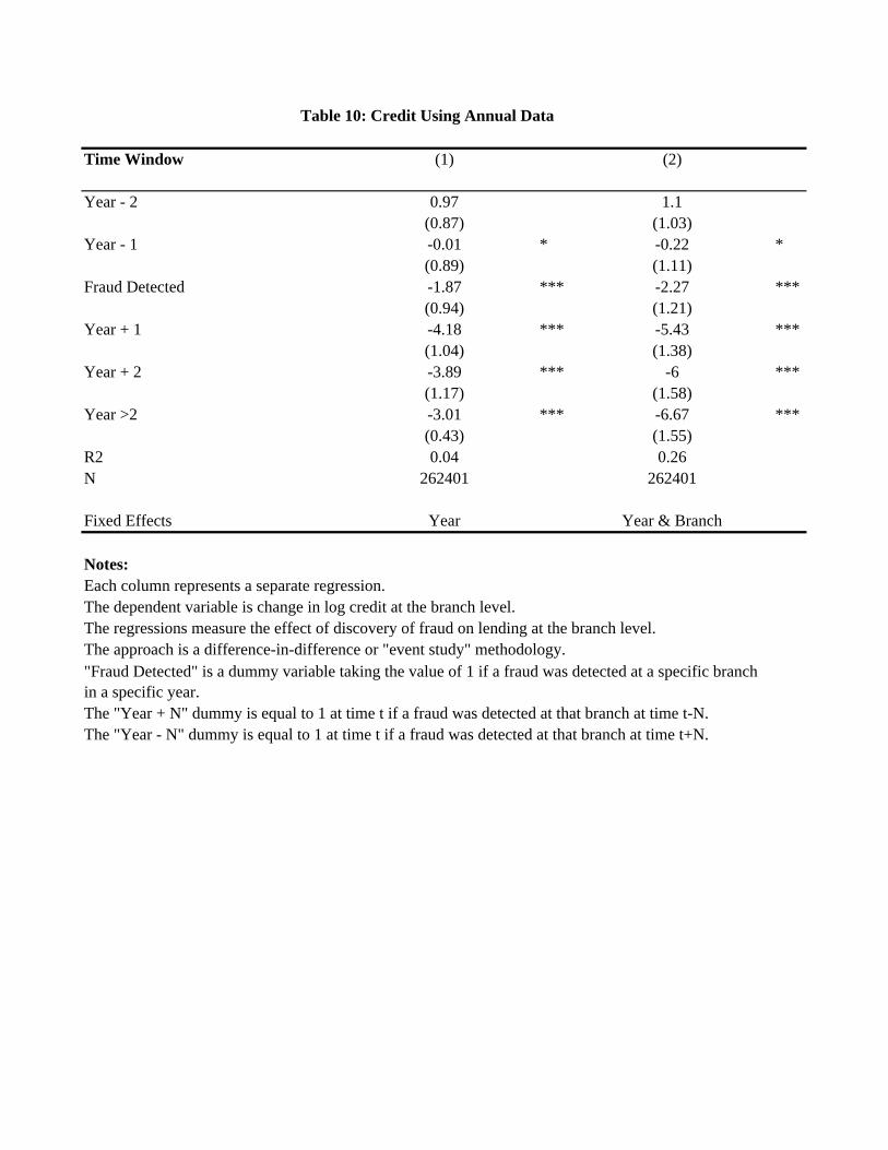
Time Window (1) (2)

Year - 2 0.97 1.1(0.87) (1.03)

Year - 1 -0.01 * -0.22 *(0.89) (1.11)

Fraud Detected -1.87 *** -2.27 ***(0.94) (1.21)

Year + 1 -4.18 *** -5.43 ***(1.04) (1.38)

Year + 2 -3.89 *** -6 ***(1.17) (1.58)

Year >2 -3.01 *** -6.67 ***(0.43) (1.55)

R2 0.04 0.26N 262401 262401

Fixed Effects Year Year & Branch

Notes:Each column represents a separate regression. The dependent variable is change in log credit at the branch level.The regressions measure the effect of discovery of fraud on lending at the branch level.The approach is a difference-in-difference or "event study" methodology.

The "Year + N" dummy is equal to 1 at time t if a fraud was detected at that branch at time t-N.The "Year - N" dummy is equal to 1 at time t if a fraud was detected at that branch at time t+N.

Table 10: Credit Using Annual Data

"Fraud Detected" is a dummy variable taking the value of 1 if a fraud was detected at a specific branch in a specific year.

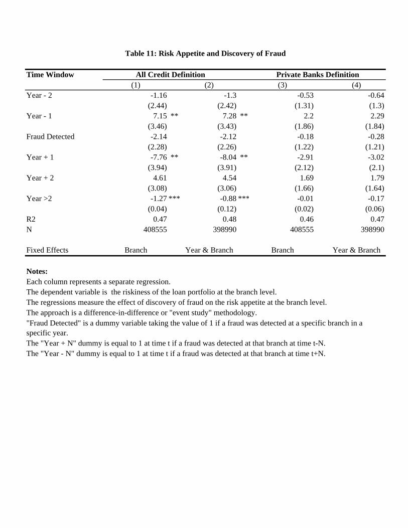
Time Window(1) (2) (3) (4)

Year - 2 -1.16 -1.3 -0.53 -0.64(2.44) (2.42) (1.31) (1.3)

Year - 1 7.15 ** 7.28 ** 2.2 2.29(3.46) (3.43) (1.86) (1.84)

Fraud Detected -2.14 -2.12 -0.18 -0.28(2.28) (2.26) (1.22) (1.21)

Year + 1 -7.76 ** -8.04 ** -2.91 -3.02(3.94) (3.91) (2.12) (2.1)

Year + 2 4.61 4.54 1.69 1.79(3.08) (3.06) (1.66) (1.64)

Year >2 -1.27 *** -0.88 *** -0.01 -0.17(0.04) (0.12) (0.02) (0.06)

R2 0.47 0.48 0.46 0.47N 408555 398990 408555 398990

Fixed Effects Branch Year & Branch Branch Year & Branch

Notes:Each column represents a separate regression. The dependent variable is the riskiness of the loan portfolio at the branch level.The regressions measure the effect of discovery of fraud on the risk appetite at the branch level.The approach is a difference-in-difference or "event study" methodology.

The "Year + N" dummy is equal to 1 at time t if a fraud was detected at that branch at time t-N.The "Year - N" dummy is equal to 1 at time t if a fraud was detected at that branch at time t+N.

All Credit Definition Private Banks Definition

Table 11: Risk Appetite and Discovery of Fraud

"Fraud Detected" is a dummy variable taking the value of 1 if a fraud was detected at a specific branch in a specific year.

Time Window(1) (2) (3) (4) (5) (6)

Year - 2 0.85 0.79 -0.64 -0.45 -0.39 1.74(0.82) (0.92) (1.36) (1.65) (0.85) (0.76)

Year - 1 0.08 -0.42 -0.54 -0.98 -0.8 1.96(0.85) (0.97) (1.39) (1.72) (0.89) (0.8)

Fraud Detected -2.42 *** -3.03 *** 4.39 *** 5.99 *** 2.9 *** 5.56(0.89) (1.03) (1.53) (1.88) (0.95) (0.87)

Year + 1 -4.03 *** -4.66 *** -2.01 -1.58 5.89 *** 8.91(0.97) (1.15) (1.59) (2.05) (1.03) (0.96)

Year + 2 -4.52 *** -5.33 *** 4.37 *** 4.09 * 6.83 *** 9.65(1.03) (1.24) (1.66) (2.18) (1.13) (1.06)

Year >2 -3.48 *** -4.72 *** -0.81 -0.75 7.39 *** 9.51(0.39) (1.09) (0.57) (1.88) (0.43) (0.92)

R2 0.04 0.2 0.01 0.29 0.08 0.49N 357266 357266 154139 154139 417314 417314

Fixed Effects Year Year & Branch Year Year & Branch Year Year & Branch

Notes:Each column represents a separate regression. The dependent variable is change in log credit at the branch level, change in log bad credit or share of bad loans.The regressions measure the effect of discovery of fraud on lending at the branch level.The approach is a difference-in-difference or "event study" methodology.

The "Year + N" dummy is equal to 1 at time t if a fraud was detected at that branch at time t-N.The "Year - N" dummy is equal to 1 at time t if a fraud was detected at that branch at time t+N.

"Fraud Detected" is a dummy variable taking the value of 1 if a fraud was detected at a specific branch in a specific year.

Table 12: Bad Credit and Discovery of Fraud

Share Bad Loans Change in Log Bad CreditChange in Log Credit

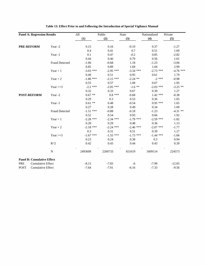
Panel A: Regression Results All Public State Nationalized Private(1) (2) (3) (4) (5)

PRE-REFORM Year -2 0.15 0.16 -0.19 0.37 -1.270.4 0.41 0.7 0.51 1.69

Year -1 0.1 0.47 -0.2 0.85 -2.820.44 0.46 0.79 0.56 1.61

Fraud Detected -1.06 -0.68 1.18 -1.23 -3.060.85 0.89 1.69 1.04 2.99

Year + 1 -3.03 *** -2.95 *** -3.34 *** -2.73 *** -4.76 ***0.49 0.51 0.95 0.61 1.79

Year + 2 -1.86 *** -2.15 *** -2.24 ** -2 *** -0.980.55 0.57 1.08 0.67 1.95

Year >=3 -2.2 *** -2.05 *** -1.6 ** -2.03 *** -3.25 **0.32 0.33 0.67 0.39 1.27

POST-REFORM Year -2 0.67 ** 0.8 *** -0.68 1.42 *** -0.380.29 0.3 0.53 0.36 1.05

Year -1 0.61 ** 0.48 -0.54 0.95 *** 1.650.27 0.28 0.49 0.34 1.00

Fraud Detected -1.51 *** -0.88 -0.18 -1.23 -4.31 **0.52 0.54 0.93 0.66 1.92

Year + 1 -2.28 *** -2.34 *** -1.79 *** -2.59 *** -1.820.28 0.29 0.48 0.36 1.13

Year + 2 -2.18 *** -2.24 *** -2.46 *** -2.07 *** -1.770.3 0.31 0.51 0.39 1.17

Year >=3 -1.67 *** -1.55 *** -1.73 *** -1.44 *** -1.660.23 0.24 0.38 0.3 0.94

R^2 0.42 0.43 0.44 0.43 0.39. . . . .

N 2493609 2260733 651619 1609114 224573

Panel B: Cumulative EffectPRE Cumulative Effect -8.15 -7.83 -6 -7.99 -12.05POST Cumulative Effect -7.64 -7.01 -6.16 -7.33 -9.56

Table 13: Effect Prior to and Following the Introduction of Special Vigilance Manual