STOCHASTIC ANALYSIS TO ASSESS THE PERFORMANCE OF PELTON WHEEL TEST...

IJRET: International Journal of Research in Engineering and Technology eISSN: 2319-1163 | pISSN: 2321-7308

_______________________________________________________________________________________

Volume: 05 Special Issue: 13 | ICRAES-2016 | Sep-2016, Available @ http://www.esatjournals.org 139

STOCHASTIC ANALYSIS TO ASSESS THE PERFORMANCE OF

PELTON WHEEL TEST RIG KEEPING SPEED CONSTANT

Pranav Kulkarni1, Vaibhavi Naik

2, Neena Panandikar

3

Abstract Hydraulic Turbines are being used since the ancient times to harness the energy stored in flowing streams, rivers and lakes. The

oldest and the simplest form of a hydraulic turbine was the waterwheel used for grinding grains. The basic idea of a Pelton Wheel

Turbine is derived from this ancient waterwheel.

Pelton wheel is the only hydraulic turbine of the impulse type in common use. It is named after the American engineer Laster A.

Pelton, who contributed much to its development around the year 1880. Therefore, this machine is known as Pelton Turbine or

Pelton Wheel. Pelton Wheels are the preferred turbine for hydro-power when the available water source has relatively high

hydraulic head at low flow rates.

In the present study, a complete analysis of the Pelton Wheel Test Rig with brake drum loading made available on college campus

is carried out. The major input and output parameters along with their working ranges are identified. Stochastic analysis using

Monte Carlo’s simulation is carried out by randomly generating a design matrix and thus calculating the responses using pre-

determined equations. Response Surface Methodology is adapted to identify the optimal set of inputs and also generate input-

output relations.

Furthermore, a design matrix is generated by taking practical readings on the Test Rig keeping speed constant and the respective

outputs are calculated. Similar to the stochastic study, Response Surface Methodology is adapted by inputting the design matrix in

a design expert software. Input-output relations are generated and also the optimal set of input parameters are determined using

this software.

Keywords: Stochastic analysis, Monte Carlo’s simulation, Response Surface Methodology

----------------------------------------------------------------------***--------------------------------------------------------------------

1. INTRODUCTION

Hydraulic Turbines have a row of blades fitted to the

rotating shaft or a rotating plate. Flowing liquid, mostly

water, when passedthrough the hydraulic turbine strikes the

blades of the turbine and makes the shaft rotate. While

flowing through the hydraulic turbine the velocity and

pressure of the liquid reduces, resulting in the development

of torque hence rotating the turbine shaft. There are different

forms of hydraulic turbines in use depending on the

operational requirements. For every specific use, a particular

type of hydraulic turbine provides the optimum output.

The basic components of a Pelton Turbine include reservoir,

penstock, check valve, nozzle, spear, rotating wheel (runner)

with buckets/vanes, casing and output shaft as shown in

Figure 1.

Fig 1: Components of a Pelton Turbine.

The basic working principle of Pelton Turbine is simple:

when a high speed water jet injected through a nozzle hits

the buckets of Pelton Wheel it induces an impulsive force.

This force makes the turbine rotate. The rotating shaft runs a

generator and produces electricity.

Nozzles direct forceful, high-speed streams of water against

a rotary series of spoon-shaped buckets, also known as

impulse blades, which are mounted around the

circumferential rim of a drive wheel, also called a runner. As

the water jet hits the contoured bucket-blades, the direction

of water velocity is changed to follow the contours of the


_______________________________________________________________________________________


bucket. Water impulse energy exerts torque on the bucket-

wheel system thus spinning the wheel. The water stream

itself does a "U-turn" and exits at the outer sides of the

bucket. While doing so it decelerates to a lower velocity. In

the process, the water jet's momentum is transferred to the

wheel and thence to the turbine. A very small percentage of

the water jet's original kinetic energy remains in the water.

This helps the bucket to be emptied at the same rate it is

filled, and thereby allows the high-pressure input flow to

continue uninterrupted, without wastage of energy.

Typically, two buckets are mounted side-by-side on the

wheel, which splits the water jet into two equal streams.

This balances the side-load forces on the wheel and helps to

ensure smooth, efficient transfer of momentum of the fluid

jet of water to the turbine wheel. [1]

In this project we aim to generate response equations in

terms of input variables and find the optimal set of input

parameters using Response Surface Methodology (RSM) for

constant speed readings. Furthermore, the optimal set of

inputs are tested on the Test Rig available and respective

responses arecalculated using pre-determined equations and

compared with the values obtained through RSM. Thus the

error is determined. Response Surface methodology is

carried out using Design Expert 10 software by stat-ease.

2. MATERIALS AND METHODS

The Pelton Turbine used is a laboratory test rig designed and

fabricated for engineering graduate and post graduate

student’s laboratory experimental purpose. Some of the

aspects of the turbine used in the present investigation are

described below:

The Pelton turbine used in the present investigation is

similar to the conventional turbine which consists of three

basic components: a stationary inlet nozzle, a runner and a

casing. The runner consists of multiple buckets mounted on

a rotating wheel. The inlet nozzle jet strikes the buckets and

imparts momentum. The buckets are shaped in a manner to

divide the flow in half and turn its relative velocity vector by

nearly 180°. The turbine experimental facility supplied is

fitted with a centrifugal pump set, a brake drum and belt

system, a spring balance, a tachometer, pressure valves, a

sump tank and a nozzle arranged in such a way such that the

whole unit functions as a re-circulating water system. The

centrifugal pump set supplies the water from sump tank to

the turbine through control valve. [2]

The loading of the

turbine is achieved by brake drum connected to spring

balance. A V-notch arrangement is used to find the

discharge of this system. Specifications of the Pelton Wheel

Test Rig are provided below in Table 1.

Table 1: Specifications of the Pelton Wheel Turbine.

Supply pump

Specifications

50Hz, AC, 440V,

7.5hp, 3ph

Turbine Mean Diameter 259mm

Number of buckets 20

Diameter of Jet 18mm

Head 100m

Loading Brake drums

Maximum shaft output 1.5kW, V-

notch=60⁰, Cd=0.6

Determining Turbine Parameters

The first step involves finding the major input and output

parameters of the Pelton Wheel Turbine. Parameters are

widely divided into three categories:

1. Design Parameters

2. Input Parameters

3. Output Parameters

In this study we do notconsider the design parameters such

as number of buckets, diameter of jet, diameter of runner

and other such parameters.

By understanding the past studies and the working of Pelton

Wheel the following major input and output parameters are

identified and listed in Table 2. [4]

Table 2: Input and Output Parameters

Input Parameters Output Parameters

head over notch(h in cm) Discharge(Q in m3/s)

Pressure(P in kg/cm2) Hydraulic Pressure

(Phyd in kW)

Speed of Runner(N in

rpm)

Brake Power(BP in

kW)

Load(F in kgf) Efficiency(η in %)

The head over the V-notch is measured using a metric scale

attached along the V-notch which is then used to calculate

the discharge using the pre-determined equation. Pressure in

the pipeline is measure using the pressure valve and

indicated on a pressure dial. Speed of runner is measured

using the tachometer and is indicated on a digital display.

Loading is done using the brake drum system with a spring

balance used to measure the loading and indicated on an

analogue display.

Pre-Determined Input-Output Relations

The output responses are calculated using pre-determined

theoretical equations. These equations are obtained from

reference sources and are shown below. [3]

1. Head on turbine (H in m of water) = 10 ×P

2. Discharge (Q in m3/s) =

8

15Cd tan(θ/2)h

5/2

3. Hydraulic Pressure (Phyd in Kw) = 𝑄𝜌𝑔𝐻

1000

4. Brake Power (BP in kW) = 2ᴨ𝑁𝐹𝑟𝑔

60×1000

5. Turbine efficiency (η in %) = (BP/ Phyd) x 100

Where,

Θ is the degree of notch = 60⁰ g is acceleration due to gravity = 9.81m

2/s

Cd is the coefficient of discharge = 0.6

Ρ is the density of water = 1000 kg/m3

r is the radius of brake drum = 0.15m


_______________________________________________________________________________________


Determining Limits of Input Variables

The analytical procedure first requires to identify and

specify the domain in which the experiment is to be

conducted, that is, the limits of the input parameters. These

are decided based on previous historical data and the

specifications of the Test Rig. A lower limit and upper limit

are established for each of the input variables. The values

are then varied within these limits to generate respective

responses. Thus the following limits were considered based

on turbine specifications and historic data:

head over notch (h) varies from 8 to 13 cm

Speed (N) of runner varies from 700 to 1200 rpm

Load (F) on the output shaft varies from 0.1 to 9 kgf

Inlet pressure (P) varies from 1 to 5 kg/cm2

Stochastic Analysis

A stochastic systemis one that is unpredictable due to the

influence of a random variable. Researchers refer to physical

systems in which they are uncertain about the values of

parameters, measurements, expected input and disturbances

as stochastic systems. In probability theory, a purely

stochastic system is one whose state is randomly

determined, having a random probability distribution or

pattern that may be analysed statistically but may not be

predicted precisely. In this regard, it can be classified as

non-deterministic so that the subsequent state of the system

is determined probabilistically. [1]

Thus, we use stochastic approach to generate a design

matrix of random input values and its respective responses

to take into consideration uncertainties which may be caused

due to vibration, friction and other such factors. Thousand

readings of randomly generated input values are taken and

respective responses are generated. This is done by Monte-

Carlo’s simulation using excel sheet.

Monte Carlo’s Simulation using Excel

Monte Carlo method is a broad class of computational

algorithms that rely on repeated random sampling to obtain

numerical results. Their essential idea is using randomness

to solve problems that might be deterministic in principle. It

shows the extreme possibilities as well as all middle order

consequences. Monte Carlo simulation performs risk

analysis by building models of possible results by

substituting a probability distribution for any factor that has

inherent uncertainty. It then calculates results over and over,

each time using a different set of random values from the

probability functions. Depending upon the number of

uncertainties and the ranges specified for them, a Monte

Carlo simulation could involve thousands or tens of

thousands of recalculations before it is complete. Monte

Carlo simulation produces distributions of possible outcome

values. [1]

Monte Carlo methods vary, but tend to follow a particular

pattern:

1. Define a domain of possible inputs.

2. Generate inputs randomly from a probability

distribution over the domain.

3. Perform a deterministic computation on the inputs.

4. Aggregate the results.

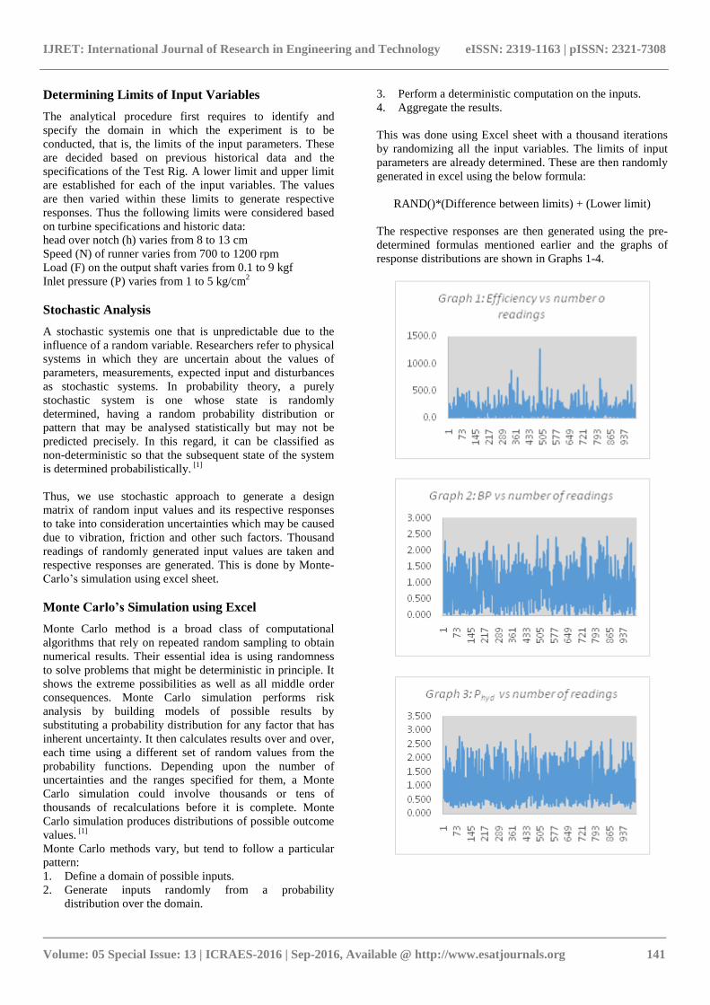
This was done using Excel sheet with a thousand iterations

by randomizing all the input variables. The limits of input

parameters are already determined. These are then randomly

generated in excel using the below formula:

RAND()*(Difference between limits) + (Lower limit)

The respective responses are then generated using the pre-

determined formulas mentioned earlier and the graphs of

response distributions are shown in Graphs 1-4.


_______________________________________________________________________________________


From these graphs we can see the responses calculated by

randomized input values. Notice in Graph 4, Discharge is

within a certain band as it is only function of head over

notch. Thus it is in a bandwidth of a certain constant

multiplied to the bandwidth of head over notch.

Response Surface Methodology (RSM)- using

Design Expert Software

Response Surface Methodology is a collection of

mathematical and statistical techniques for empirical model

building. The objective is to optimize a response which is

influenced by several independent input variables.

Thus in this study we use RSM to generate response

equations in terms of input parameters and also to find the

optimal set of inputs to get an optimal output. This

procedure is conducted for stochastic as well as Test Rig

design matrices using Design Expert 10 software by stat

ease.The 3-D graphs generated for the ouputs using

Response Surface Methodology through Design Expert

software for the stochastic design matrix are shown in

Figures2-6.

Design Matrix from Test Rig

Experiments are conducted on the Pelton Wheel Test Rig

keeping speed constant. Twenty-six readings in five sets are

taken using constant speed in the range 700 to 1200. The

readings are shown in Table 3.

Design of Experiment Procedure

1. Designing of experiments for adequate and reliable

measurement of the response.

2. Developing a mathematical model of the second-order

response surface with the best fittings.

3. Finding the optimal set of parameters that produce a

maximum or minimum value of response.

4. Representing the direct and interactive effects of process

parameters through two or three dimensional plots.

If all controlled variables are assumed to be measurable then

the response surface can be expressed as:

𝒚=𝒇 (𝒙1, 𝒙𝟐, 𝒙𝟑……. 𝒙𝒌)

where ‘y’ is the output and ‘xi’ are the input variables called

factors, where i=1,2…k.

The goal in this aspect of the study is to optimize the

response variable ‘y’. The independent variables are

assumed to be continuous and controllable by the

experiments with negligible errors. A reasonable

approximation for the true functional relationship between

independent variables and the response surface is desired.

Different models can be used in RSM as per the fit of the

model example: linear, quadratic, cubic, 2FI and other such

models. [3]

3. RESULTS

Test Rig readings of Pelton Wheel Turbine for different

values of constant speed are shown in Table 3. As expected,

from the table we can infer that to maintain constant speed

as the Load is increased the Pressure too needs to be

increased. Thus, Pressure is directly proportional to Load,

considering Speed is constant. Also, it can be noticed that

the Efficiency of the turbine increases with the increase in

Load up to a certain limit after which it starts declining.

The 3-D plots of the responses generated using Design

Expert Software are shown in Figures 7-11. The input-

output relations are also generated by using Response

Surface Methodology which help us to calculate the outputs

directly by knowing the input values.

Relation between Head and Input Parameters

It is seen that a Head fits a linear model with the input

parameters as shown in the equation below:

H = (1.730*E-014) + (2.285*E-017*N) + (10*P)

+ (1.918*E-015*F) - (3.751*E-013*h)

Relation between Discharge and Input Parameters

Discharge fits a quadratic model with the input parameters

which is shown in equation below:

Q = (3.483*E-004) - (3.485*E-006*N)

- (1.683*E-004*F) + (8.619*E-003*h)

- (1.771*E-007*N*F) + (7.091*E-005*N*h)

+ (3.054*E-003*F*h) - (2.335*E-009*N2)

-(4.443*E-006*F2)

Relation between Hydraulic Pressure and Input

Parameters

Hydraulic Pressure fits a 2FI model with the input

parameters which is further modified to get the equation

below:

Phyd = (1.949) - (1.940*E-003*N) - (0.513*P)

- (0.066*F) - (19.005*h) - (1.882*E-004*N*P)

+ (7.276*E-005*N*F) + (0.0191*N*h)

+(9.072*P*h)


_______________________________________________________________________________________


Relation between Brake Power and Input

Parameters

Brake power has a large maximum to minimum ratio thus a

logarithmic transformation is appliedproviding a 2FI model

fit with the input parameters as shown in the equation

below:

Log10(BP) = - (1.860) + (0.201*P) + (0.535*F)

-(0.083*P*F)

Relation between Efficiency and Input Parameters

Efficiency also has a large maximum to minimum ratio thus

a logarithmic transformation is applied provided a 2FI

model fit with the input parameters as shown in the equation

below:

Log10(η) = (2.012) + (9.077*E004*N) + (0.013 *P)

+(0.517*F) - (18.935 * h) - (0.0713 * P * F)

Fig 2: Shows variation of Head against Pressure and head

over notch

Fig 3: Shows variation of Phyd against Pressure and head

over notch

Fig 4: shows variation of Discharge against Pressure and

head over notch

Fig 5: Shows variation off Efficiency against Pressure and

head over notch

Fig 6: Shows variation of BP against Pressure and head

over notch

Design-Expert® SoftwareFactor Coding: ActualHead (m of water)

49.9723

10.0384

X1 = A: head over nocthX2 = B: Pressure

Actual FactorsC: Speed = 1200D: Load = 4.55

1

2

3

4

5

0.08

0.09

0.1

0.11

0.12

0.13

0.14

10

20

30

40

50

Head (

m o

f w

ate

r)

A: head over nocth (m)B: Pressure (kg/cm2)

Design-Expert® SoftwareFactor Coding: ActualOriginal ScalePhyd (kW)

2.87532

0.161685



1

2

3

4

5

0.08

0.09

0.1

0.11

0.12

0.13

0.14

0

0.5

1

1.5

2

2.5

3

Phyd (

kW

)


Design-Expert® SoftwareFactor Coding: ActualDischarge (m3/s)

0.00599245

0.00148282



1

2

3

4

5

0.08

0.09

0.1

0.11

0.12

0.13

0.14

0.001

0.002

0.003

0.004

0.005

0.006

0.007

Dis

charg

e (

m3/s

)


Design-Expert® SoftwareFactor Coding: ActualOriginal ScaleEfficiency (%)

1277.64

0.957742



1

2

3

4

5

0.08

0.09

0.1

0.11

0.12

0.13

0.14

0

200

400

600

800

1000

1200

1400

Eff

icie

ncy (

%)

A: head over nocth (m)

B: Pressure (kg/cm2)

Design-Expert® SoftwareFactor Coding: ActualOriginal ScaleBP (kW)

2.46355

0.0197182



1

2

3

4

5

0.08

0.09

0.1

0.11

0.12

0.13

0.14

0

0.5

1

1.5

2

2.5

BP

(kW

)



_______________________________________________________________________________________


Table 3: Test rig readings for constant speed

INPUTS OUPUT PARAMETERS

Speed

(rpm)

Pressure

(kg/cm2)

Load

(kgf)

head over

notch (m)

Head (m

of water)

Discharge

(m3/s)

Phyd

(kW)

BP

(kW)

Efficiency

(%)

700 2.6 0.725 0.087 26 0.0018 0.4660 0.0782 16.77

700 3.2 1.25 0.0919 32 0.0021 0.6577 0.1348 20.49 700 4 1.05 0.0932 40 0.0022 0.8515 0.1132 13.29

700 4.5 1.875 0.094 45 0.0022 0.9786 0.2021 20.66

700 5 2 0.0962 50 0.0023 1.1521 0.2156 18.72 800 1 0.15 0.1061 10 0.0030 0.2944 0.0185 6.28

800 1.8 0.9 0.1058 18 0.0030 0.5261 0.1109 21.08 800 2.4 2.9 0.1058 24 0.0030 0.7015 0.3573 50.94

800 2.7 2 0.1066 27 0.0030 0.8042 0.2464 30.64 800 3.1 3.8 0.1153 31 0.0037 1.1234 0.4682 41.68

800 3.8 5 0.1223 38 0.0043 1.5956 0.6161 38.61

800 5.4 8.5 0.126 54 0.0046 2.4429 1.0473 42.87 900 1.6 0.1 0.1127 16 0.0035 0.5477 0.0139 2.53

900 1.8 0.7 0.1156 18 0.0037 0.6565 0.0970 14.78 900 2.4 2 0.1186 24 0.0040 0.9333 0.2772 29.71

900 2.6 2.8 0.1205 26 0.0041 1.0520 0.3881 36.89

900 3.3 3.9 0.1236 33 0.0044 1.4228 0.5406 38.00 1000 2 0.2 0.116 20 0.0038 0.7358 0.0308 4.19

1000 2.1 0.5 0.12 21 0.0041 0.8409 0.0770 9.16 1000 3.2 3.45 0.132 32 0.0052 1.6262 0.5314 32.68

1000 3.8 5 0.135 38 0.0055 2.0427 0.7701 37.70

1000 4.2 5.75 0.138 42 0.0058 2.3852 0.8856 37.13 1100 2.6 1.9 0.1216 26 0.0042 1.0762 0.3219 29.91

1100 3.6 3.05 0.1244 36 0.0045 1.5774 0.5167 32.76 1100 4.2 4.2 0.125 42 0.0045 1.8625 0.7116 38.20

1100 4.6 4.75 0.126 46 0.0046 2.0810 0.8047 38.67

Fig 7: Shows variation of Head against Pressure and Speed

Fig 8: Shows variation of Discharge against Pressure and

Speed

Design-Expert® SoftwareFactor Coding: ActualDischarge (m3/s)

0.00578909

0.00182688

X1 = A: SpeedX2 = B: Pressure

Actual FactorsC: Load = 4.55D: head over notch = 0.105

1

2

3

4

5

700

800

900

1000

1100

1200

0.001

0.002

0.003

0.004

0.005

0.006

Dis

charg

e (

m3/s

)

A: Speed (rpm)



_______________________________________________________________________________________


Fig 9: Shows variation of Phyd against Pressure and Speed

Fig 10: Shows variation of BP against Pressure and Speed

Fig 11: Shows variation of Efficiency against Pressure and

Speed

Optimal Solution

By performing optimization for the test rig design matrix in

design expert 10 software it is determined that the optimum

efficiency is η=96.96% with a desirability of 1.

The respective optimal set of inputs are:

Speed, N= 1009.74rpm

Pressure, P= 1.6666 kg/cm2

Load, F= 2.102 Kgf

head over notch, h= 0.096 m

The above set of input parameters were experimented on the

Test Rig and respective outputs were calculated using the

pre-determined equations. The value of Efficiency was

found out to be, η=84.86%

4. CONCLUSION

Thus, input-output relations were generated and verified.

The optimal input set was also identified and the error is

calculated,

Error, e= 96.96 – 84.86 = 12.1%

This error may be caused due to frictional loses along pipe

lengths and bends and other frictional loses.

REFERENCES

[1]. https://en.wikipedia.org/wiki/Main_Page Wikipedia, the

free encyclopaedia, Pelton Wheel, Monte Carlo’s Simulation

and Water Turbine.

[2]. Turkish Journal of Engineering, Science and

Technology, Assessment on the Performance of Pelton

Turbine Test Rig Using Response Surface Methodology by

Alok Ku Nandaa, Soumya Dashb, R. Bhima Raoc, Satya Sai

Srikantd, 2013.

[3]. Kadambi V. Manohar Prasad: An introduction to energy

conversion, Volume III, New Age Publications, 1997.

[4]. R K Bansal, (2010), A Textbook of fluid mechanics and

hydraulic machines, Laxmi Publications, 9th Edition (2010).

Design-Expert® SoftwareFactor Coding: ActualPhyd (kW)

2.44288

0.294354



1

2

3

4

5

700

800

900

1000

1100

1200

0

0.5

1

1.5

2

2.5

Phyd (

kW

)

A: Speed (rpm)B: Pressure (kg/cm2)

Design-Expert® SoftwareFactor Coding: ActualOriginal ScaleBP (kW)

1.04732

0.0138615



1

2

3

4

5

700

800

900

1000

1100

1200

0

5

10

15

20

BP

(kW

)

A: Speed (rpm)B: Pressure (kg/cm2)

Design-Expert® SoftwareFactor Coding: ActualOriginal ScaleEfficiency (%)

50.9389

2.53104



1

2

3

4

5

700

800

900

1000

1100

1200

0

1000

2000

3000

4000

Eff

icie

ncy (

%)

A: Speed (rpm)


STOCHASTIC ANALYSIS TO ASSESS THE PERFORMANCE OF PELTON WHEEL TEST...

Documents

Transcript of STOCHASTIC ANALYSIS TO ASSESS THE PERFORMANCE OF PELTON WHEEL TEST...