A model estimate on the effect of anthropogenic land cover ... · Anthropogenic land cover change...
148
M a x - P l a n c k - I n s t i t u t f ü r M e t e o r o l o g i e Max Planck Institute for Meteorology Julia Pongratz Berichte zur Erdsystemforschung Reports on Earth System Science 68 2009 A model estimate on the effect of anthropogenic land cover change on the climate of the last millennium
Transcript of A model estimate on the effect of anthropogenic land cover ... · Anthropogenic land cover change...
M a x - P l a n c k - I n s t i t u t f ü r M e t e o r o l o g i e Max Planck Institute for Meteorology
Julia Pongratz
Berichte zur Erdsystemforschung Reports on Earth System Science
682009
A model estimate on the effect
of anthropogenic land cover change
on the climate of the last millennium

Julia Pongratzaus München
Reports on Earth System Science
Berichte zur Erdsystemforschung 682009
682009
ISSN 1614-1199
A model estimate on the effect of anthropogenic land cover change on the climate of the last millennium
Dissertation zur Erlangung des Doktorgrades der Naturwissenschaftenim Department Geowissenschaften der Universität Hamburg
vorgelegt von
Hamburg 2009

Julia PongratzMax-Planck-Institut für Meteorologie Bundesstrasse 53 20146 Hamburg Germany
ISSN 1614-1199
Als Dissertation angenommen vom Department Geowissenschaften der Universität Hamburg
auf Grund der Gutachten von Prof. Dr. Martin Claußenund Dr. Christian H. Reick
Hamburg, den 29. April 2009Prof. Dr. Jürgen Oßenbrügge Leiter des Department Geowissenschaften
Julia PongratzHamburg 2009
A model estimate on the effect of anthropogenic land cover change on the climate of the last millennium

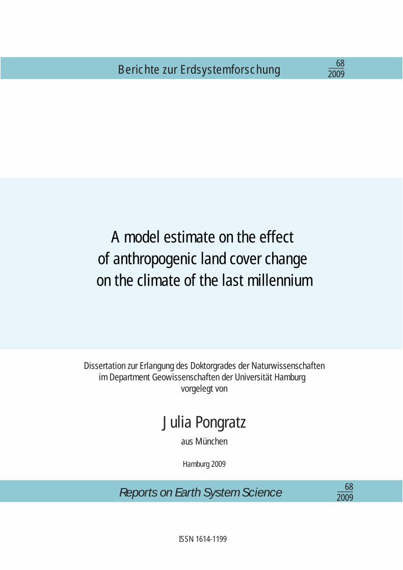
Cover picture
The image on the front page illustrates the expansion of agriculture in the lastmillennium and the associated increasing influence of humankind on climate andthe carbon cycle. From back to front: Late-medieval farmers1 on the cropland mapof the year 1500. Farmer of the late preindustrial period2 on the cropland map ofthe year 1850. Modern plough3 on the cropland map of the year 1992. Eachmolecule of CO2 stands for approximately 100 Tg C/year primary emissions in therespective year, indicating emissions of 40, 320, and 900 Tg C/year for the threeyears. Cropland maps and CO2 estimates are described in Chapters 2 and 4,respectively.
Picture credits:1 Modified from Project Gutenberg. Illustration probably from the early 16thcentury with legend “God Spede ye Plough, and send us Korne enow”.2 modified from a sketch by Vincent van Gogh, 1883.3 modified from Rasbak, Wikimedia Commons, licensed under “GNU-Lizenz furfreie Dokumentation” (Licence text seehttp://en.wikipedia.org/wiki/Wikipedia:Text of the GNU Free Documentation License).
i
Contents
Abstract 1
List of Abbreviations 3
1 Introduction 51.1 The importance of anthropogenic land cover change for climate . . . 61.2 “Anthropogenic land cover change” - definition and quantification . 81.3 A brief summary of the history of agriculture . . . . . . . . . . . . . 101.4 The last millennium . . . . . . . . . . . . . . . . . . . . . . . . . . . 121.5 Biosphere-atmosphere interactions and goals of this study . . . . . . 14
2 A Reconstruction of Global Agricultural Areas and Land Cover forthe Last Millennium 212.1 Introduction . . . . . . . . . . . . . . . . . . . . . . . . . . . . . . . . 222.2 Step 1: Adaptation of agricultural data since AD 1700 . . . . . . . . 23
2.2.1 Cropland . . . . . . . . . . . . . . . . . . . . . . . . . . . . . 242.2.2 Pasture . . . . . . . . . . . . . . . . . . . . . . . . . . . . . . 25
2.3 Step 2: Reconstruction of agricultural areas AD 800 to 1700 . . . . . 252.4 Step 3: From agricultural areas to land cover . . . . . . . . . . . . . 282.5 Assessing uncertainty and validity . . . . . . . . . . . . . . . . . . . 30
2.5.1 Inclusiveness of the millennium reconstruction . . . . . . . . 302.5.2 Validation of the base data AD 1700 to 1992 . . . . . . . . . 302.5.3 Uncertainty of the population data . . . . . . . . . . . . . . . 312.5.4 Effects of agrotechnical improvements . . . . . . . . . . . . . 32
2.6 Changes in land cover AD 800–1992 . . . . . . . . . . . . . . . . . . 342.6.1 Europe and Former Soviet Union . . . . . . . . . . . . . . . . 382.6.2 North Africa/Middle East . . . . . . . . . . . . . . . . . . . . 402.6.3 South Asia and Southeast Asia . . . . . . . . . . . . . . . . . 402.6.4 China . . . . . . . . . . . . . . . . . . . . . . . . . . . . . . . 422.6.5 Pacific Developed . . . . . . . . . . . . . . . . . . . . . . . . . 422.6.6 Tropical Africa . . . . . . . . . . . . . . . . . . . . . . . . . . 432.6.7 The Americas . . . . . . . . . . . . . . . . . . . . . . . . . . . 44
2.7 Conclusion . . . . . . . . . . . . . . . . . . . . . . . . . . . . . . . . 45
ii Contents
3 Radiative Forcing from Anthropogenic Land Cover Change sinceAD 800 473.1 Introduction . . . . . . . . . . . . . . . . . . . . . . . . . . . . . . . . 473.2 Radiative forcing calculations . . . . . . . . . . . . . . . . . . . . . . 493.3 Results . . . . . . . . . . . . . . . . . . . . . . . . . . . . . . . . . . . 493.4 Discussion . . . . . . . . . . . . . . . . . . . . . . . . . . . . . . . . . 513.5 Conclusions . . . . . . . . . . . . . . . . . . . . . . . . . . . . . . . . 53
4 Effects of Anthropogenic Land Cover Change on the Carbon Cycleof the Last Millennium 554.1 Introduction . . . . . . . . . . . . . . . . . . . . . . . . . . . . . . . . 564.2 Methods . . . . . . . . . . . . . . . . . . . . . . . . . . . . . . . . . . 58
4.2.1 Model . . . . . . . . . . . . . . . . . . . . . . . . . . . . . . . 584.2.2 ALCC data . . . . . . . . . . . . . . . . . . . . . . . . . . . . 604.2.3 Simulation protocol . . . . . . . . . . . . . . . . . . . . . . . 60
4.3 Primary emissions and carbon cycle feedback . . . . . . . . . . . . . 624.3.1 Overview . . . . . . . . . . . . . . . . . . . . . . . . . . . . . 624.3.2 Spatial patterns . . . . . . . . . . . . . . . . . . . . . . . . . 624.3.3 Primary emissions . . . . . . . . . . . . . . . . . . . . . . . . 634.3.4 Coupling flux . . . . . . . . . . . . . . . . . . . . . . . . . . . 67
4.4 Anthropogenic influence on the preindustrial carbon cycle and climate 694.4.1 Anthropogenic contribution to Holocene CO2 increase . . . . 694.4.2 Effect of ALCC on global mean temperatures . . . . . . . . . 724.4.3 Epidemics and warfare . . . . . . . . . . . . . . . . . . . . . . 72
4.5 Conclusions . . . . . . . . . . . . . . . . . . . . . . . . . . . . . . . . 74
5 Biogeophysical Contributions to the Effects of Anthropogenic LandCover Change 775.1 Introduction . . . . . . . . . . . . . . . . . . . . . . . . . . . . . . . . 785.2 Model and data . . . . . . . . . . . . . . . . . . . . . . . . . . . . . . 805.3 Climate response to ALCC . . . . . . . . . . . . . . . . . . . . . . . 81
5.3.1 Biogeophysical mechanisms . . . . . . . . . . . . . . . . . . . 825.3.2 Biogeochemical mechanisms . . . . . . . . . . . . . . . . . . . 86
5.4 Biogeophysically-induced changes in the carbon cycle . . . . . . . . . 865.5 Relevance of the radiative forcing concept . . . . . . . . . . . . . . . 875.6 Historical ALCC in the context of climate mitigation . . . . . . . . . 915.7 Summary and conclusions . . . . . . . . . . . . . . . . . . . . . . . . 95
6 Summary and Conclusion 996.1 Summary of methods . . . . . . . . . . . . . . . . . . . . . . . . . . . 996.2 Main findings concerning the beginning of the Anthropocene . . . . 1006.3 Main findings beyond the historical aspect . . . . . . . . . . . . . . . 1016.4 Next steps to be taken . . . . . . . . . . . . . . . . . . . . . . . . . . 102
Contents iii
Appendices 105
A Auxiliary material to the millennium land cover reconstruction 105
B Supplementary figures for biogeophysical mechanisms 109
C Error estimate for local radiative forcing from emissions 113
List of Figures 115
List of Tables 117
List of Publications 133
Acknowledgements 135

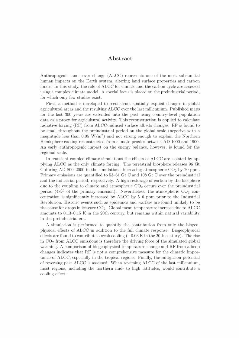
Abstract
Anthropogenic land cover change (ALCC) represents one of the most substantialhuman impacts on the Earth system, altering land surface properties and carbonfluxes. In this study, the role of ALCC for climate and the carbon cycle are assessedusing a complex climate model. A special focus is placed on the preindustrial period,for which only few studies exist.
First, a method is developed to reconstruct spatially explicit changes in globalagricultural areas and the resulting ALCC over the last millennium. Published mapsfor the last 300 years are extended into the past using country-level populationdata as a proxy for agricultural activity. This reconstruction is applied to calculateradiative forcing (RF) from ALCC-induced surface albedo changes. RF is found tobe small throughout the preindustrial period on the global scale (negative with amagnitude less than 0.05 W/m2) and not strong enough to explain the NorthernHemisphere cooling reconstructed from climate proxies between AD 1000 and 1900.An early anthropogenic impact on the energy balance, however, is found for theregional scale.
In transient coupled climate simulations the effects of ALCC are isolated by ap-plying ALCC as the only climate forcing. The terrestrial biosphere releases 96 GtC during AD 800–2000 in the simulations, increasing atmospheric CO2 by 20 ppm.Primary emissions are quantified to 53–61 Gt C and 108 Gt C over the preindustrialand the industrial period, respectively. A high restorage of carbon by the biospheredue to the coupling to climate and atmospheric CO2 occurs over the preindustrialperiod (48% of the primary emission). Nevertheless, the atmospheric CO2 con-centration is significantly increased by ALCC by 5–6 ppm prior to the IndustrialRevolution. Historic events such as epidemics and warfare are found unlikely to bethe cause for drops in ice-core CO2. Global mean temperature increase due to ALCCamounts to 0.13–0.15 K in the 20th century, but remains within natural variabilityin the preindustrial era.
A simulation is performed to quantify the contribution from only the biogeo-physical effects of ALCC in addition to the full climate response. Biogeophysicaleffects are found to contribute a weak cooling (−0.03 K in the 20th century). The risein CO2 from ALCC emissions is therefore the driving force of the simulated globalwarming. A comparison of biogeophysical temperature change and RF from albedochanges indicates that RF is not a comprehensive measure for the climatic impor-tance of ALCC, especially in the tropical regions. Finally, the mitigation potentialof reversing past ALCC is assessed: When reversing ALCC of the last millennium,most regions, including the northern mid- to high latitudes, would contribute acooling effect.

Zusammenfassung
Einen der entscheidenden Prozesse, durch die der Mensch in das Erdsystem eingreift,stellen Anderungen der Landbedeckung dar. Durch diese verandert der Mensch dieEigenschaften der Erdoberflache und beeinflusst die Kohlenstoffflusse. In der vor-liegenden Studie wird die Rolle von anthropogener Landbedeckungsanderung (“an-thropogenic land cover change”, ALCC) auf das Klima und den Kohlenstoffkreislaufmithilfe eines komplexen Klimamodells untersucht. Ein Schwerpunkt liegt dabei aufder vorindustriellen Zeit, fur die nur wenige Studien existieren.
Zuerst wird eine Methode entwickelt, um raumlich explizit Anderungen in denglobalen landwirtschaftlichen Flachen im letzten Jahrtausend und die sich darausergebende ALCC zu rekonstruieren. Landerbasierte Bevolkerungsdaten werden alsProxy fur landwirtschaftliche Aktivitat genutzt, um bestehende Karten der letz-ten 300 Jahre in die Vergangenheit zu erweitern. Mithilfe dieser Rekonstruktionwird der Strahlungsantrieb (SA) berechnet, der sich aus den ALCC-bedingtenAnderungen der Oberflachenalbedo ergibt. SA wird auf globaler Ebene fur diegesamte vorindustrielle Zeit als klein abgeschatzt (negativ mit einem Betrag vonweniger als 0.05 W/m2) und als nicht stark genug, um die Abkuhlung der nordlichenHemisphare zu erklaren, die aus Klimaproxies fur die Zeit zwischen dem Jahr 1000und 1900 rekonstruiert wurde. Auf regionaler Ebene wird jedoch ein fruher Einflussdes Menschen auf die Energiebilanz gefunden.
In transienten gekoppelten Klimasimulationen werden die Effekte von ALCCisoliert, indem ALCC als einziger Klimaantrieb im Modell verwendet wird. DieLandbiosphare verliert in diesen Simulationen etwa 96 Gt Kohlenstoff (C) uberden Zeitraum von 800 bis 2000 und erhoht dadurch die CO2-Konzentration derAtmosphare um 20 ppm. Primaremissionen werden auf 53–61 Gt C fur die gesamtevorindustrielle Zeit, und auf 108 Gt C fur die gesamte industrielle Zeit quantifiziert.Fur die vorindustrielle Zeit findet man eine starke Wiederaufnahme von Kohlenstoffin die Biosphare (48% der Primaremissionen) aufgrund der Kopplung an Klima undatmospharischem CO2. Trotzdem wird bereits vor der Industriellen Revolution dieatmospharische CO2-Konzentration durch ALCC signifikant um 5–6 ppm erhoht.Es zeigt sich, dass historische Ereignisse wie Epidemien und Kriege wahrscheinlichnicht der Grund fur CO2-Abnahmen in Eisbohrkernen sind. Die globale Mitteltem-peratur erhoht sich durch ALCC um 0.13–0.15 K im 20. Jahrhundert, bleibt aberin der vorindustriellen Zeit im Rahmen der naturlichen Variabilitat.
Eine weitere Simulation wird durchgefuhrt, die den Beitrag der biogeophysi-kalischen Effekte von ALCC zusatzlich zur vollen Klimaanderung quantifiziert.Die simulierten biogeophysikalischen Effekte bewirken einen leichten Kuhlungseffekt(−0.03 K im 20. Jahrhundert). Der CO2-Anstieg aus ALCC-Emissionen ist deshalbdie treibende Kraft hinter der simulierten Erwarmung. Ein Vergleich von biogeo-physikalischer Temperaturanderung und SA aus Albedoanderungen zeigt, dass SAbesonders in den Tropen kein vollstandiges Maß fur die Bedeutung von ALCC furdas Klima ist. Abschließend wird das Potential einer Umkehrung von ALCC zurVerminderung des Klimawandels untersucht: Bei einer Umkehr der ALCC der letz-ten tausend Jahre wurden die meisten Regionen, darunter auch die mittleren undhohen Breiten, eine Abkuhlung bewirken.

3
List of Abbreviations
ALCC anthropogenic land cover changeAOGCM atmosphere/ocean general circulation modelBVOC biogenic volatile organic compoundsC carbonDJF winter seasonECHAM5 atmosphere model applied in this studyEMIC Earth system model of intermediate complexityENSO El Nino/Southern OscillationFAO Food and Agriculture Organization of the United NationsFAOSTAT Statistical database of the Food and Agriculture Organization of
the United NationsFSU Former Soviet UnionGCM general circulation modelHAMOCC5 ocean biogeochemistry model applied in this studyHYDE History Database of the Global EnvironmentIAM Integrated Assessment ModelIPCC Intergovernmental Panel on Climate ChangeJJA summer seasonJSBACH land surface scheme applied in this studyLAI leaf area indexLUCID “Land-Use and Climate, IDentification of robust impacts” projectMAM spring seasonMPI-OM ocean and sea ice model applied in this studyNEP net ecosystem productivityNPP net primary productivityPFT plant functional typeRF radiative forcingRh heterotrophic respirationSA StrahlungsantriebSAGE Center for Sustainability and the Global Environment, University
of WisconsinSON fall seasonUNFCCC United Nations Framework Convention on Climate Change

5
Chapter 1
Introduction
If we follow the notion by Diamond [1999], the advent of agriculture was the decisivefactor that enabled cultural developments such as writing, technology, and industrialapplications that characterize the modern societies of today. Agriculture has evolvedover several thousand years: at first, few people inhabited the Earth and agriculturewas ”invented” in just a few places; later, the majority of a much larger populationworked as farmers; today, a relatively small number of farmers supports a populationof billions of people. Somewhere along this way, humans started to shape the worldin a way that scientists have coined the term “Anthropocene” for it [Crutzen andStoermer, 2000]. But, besides being the prerequisite for an industrial society thattakes decisive influence on the Earth system, agriculture may well have been initself a strong contributor to changing the Earth system. Research over the lastdecades has more and more confirmed this notion as far as agriculture at its presentextent is concerned. But the long history of agriculture implies a potentially earlyimpact on the climate, which is much less well known. This thesis follows the lastthousand years of agricultural development and investigates its influences on theclimate system from different perspectives.
The task of the present chapter is (1) to exemplarily sketch the importance ofagriculture for climate; (2) to define the subject matter of this study — agricul-ture and anthropogenic land cover change; (3) to give a synopsis of the history ofagriculture to embed the timespan under investigation in its historical context; (4)explain why exactly the timespan under investigation was chosen for this study; (5)to motivate the interest in the historical aspects of agriculture. In the last section,the different mechanisms through which anthropogenic land cover change influencesclimate will be explained. The different mechanisms will be studied in the differentparts of this thesis, and the objectives of the individual chapters will be explainedin their context. The main objectives of this thesis are highlighted by blue lines inthe following.
6 1 INTRODUCTION
1.1 The importance of anthropogenic land cover change
for climate
Anthropogenic climate change, expressed prominently in a global warming over thelast decades [Trenberth et al., 2007], is foremost driven by the increase in atmosphericgreenhouse gas concentration. Here in turn CO2 has been identified as the mainactor [Forster et al., 2007]. Anthropogenic CO2 emissions originate primarily fromthe combustion of fossil fuels and from cement manufacture, estimated to 6.4 Gtcarbon (C) per year for the 1990s; but another 1.6 Gt C per year are added byCO2 emissions from the transformation of natural vegetation to managed areas(“anthropogenic land cover change”, ALCC, see Sec. 1.2)[see Trenberth et al., 2007,for error estimates]. However, vegetation is not only a source of CO2, but also a sink:Knowing the atmospheric CO2 increase and the ocean-atmosphere CO2 flux, we caninfer that the land has been a net sink of carbon over the last decades, with anuptake of about 1.0 Gt C per year [Trenberth et al., 2007]. Comparing this againstestimates of ALCC emissions of about 1.6 Gt C, 2.6 Gt C per year must thus havebeen stored on land. This means that almost one third of total anthropogenic CO2
emissions are taken up each year by the terrestrial biosphere. The reason for a netCO2 uptake on land despite carbon loss from ALCC is, among others, increasedplant productivity initiated from the rise in CO2. This demonstrates that not onlydoes the biosphere alter climate and CO2, but climate and CO2 in turn feed back onbiospheric activity. We would like to better understand all these processes and theirinteractions since understanding is a prerequisite to take appropriate action. Onthe one hand, we need exact quantifications of the CO2 emissions in time and spacein order to determine where emissions can be reduced — emissions from fossil-fuelcombustion are very well known, but the land use carbon source has currently thelargest uncertainties in the global carbon budget [Denman et al., 2007], propagatingits uncertainties to estimates of the terrestrial sink. On the other hand, we needto understand the processes behind the sink term in order to be able to project itsfuture evolution and to possibly increase its mitigation potential.
The relevance of the biosphere and the influence humans exert on it have ini-tiated political actions on the highest international level. Several articles of theKyoto Protocol and following agreements make provisions for the inclusion of landuse, land-use change, and forestry activities as part of the efforts to implement theKyoto Protocol and contribute to the mitigation of climate change. The Intergovern-mental Panel on Climate Change (IPCC) has noted that reducing and/or preventingdeforestation is the mitigation option with the largest and most immediate carbonstock impact in the short term per area and year [Nabuurs et al., 2007]. Therefore,it is being discussed to admit to a Party’s credit the emission reduction from a re-duction in deforestation in developing countries [UNFCCC, 2007]. Already agreedon is credit for activities in the own country that lead to higher absorption of car-bon from the atmosphere or increased storage. This includes carbon sequestrationincreases above 1990 levels resulting from reduced deforestation rates or increase in

1.1 The importance of anthropogenic land cover change for climate 7
forest area, but also changes in management of forest, cropland, and grazing land,and general re-vegetation [UNFCCC, 1998]. Several tiers are proposed for quantify-ing and reporting changes in carbon stock and greenhouse gas emissions, includingspatially explicit biosphere modeling [IPCC, 2003] — the approach taken also in thepresent study.
Biosphere services are also considered to reduce the need of fossil fuels by provid-ing bioenergy. For example, substituting gasoline by first generation biofuels (mostlysugar- or oil-rich food crops) have been expected to reduce greenhouse gases becausebiofuels remove carbon from the atmosphere through the growth of the feedstockinstead of taking carbon from fossil sources [e.g., Commission of the European Com-munities, 2006]. Recent studies, however, suggest that this may not be the case: Theexpected emission savings may be outdone by the increased rates of ALCC that mayoccur when both food and energy demand need to be fulfilled in parallel by agri-cultural production [Searchinger et al., 2008]. Again, this highlights the need for aprocess understanding of source and sink terms associated with ALCC, as well asan integrated assessment thereof.
ALCC and the terrestrial biosphere are, however, relevant for climate and climatechange beyond the aspect of sources and sinks of greenhouse gases. As will be ex-plained in detail in Sec. 1.5, ALCC alters the physical properties of the land surface,and thus exerts a direct impact e.g. on water and energy fluxes. ALCC until todaymay have decreased surface temperatures by 1–2 K over midlatitude agriculturalregions [Betts, 2001, Bounoua et al., 2002, Feddema et al., 2005]. Future scenarios,anticipating large-scale deforestation in the tropical region, project warming of upto 2 K and drier hydrological conditions in the areas undergoing ALCC [DeFrieset al., 2002, Sitch et al., 2005].
From these examples of recent climate research and policy, we can conclude threepoints relevant to this study: (1) We need to improve our process understandingin order to realistically estimate current and future climatic consequences of ALCCand to assess its potential for climate change mitigation. (2) We need to investigatebiosphere-climate interactions with respect to a range of very different mechanisms.These may act in the same or in opposite directions concerning their effects onimportant climate variables, such as temperature. An integrated assessment of thedifferent mechanisms as well as their two-way interaction with climate is essential.If modeling is chosen as tool to assess these mechanisms, then a coupled setup isessential to allow the full representation of biosphere-atmosphere feedbacks. (3) Forthe present situation as well as for a range of future scenarios, the significance ofALCC for climate change has been acknowledged. Considering the long history ofagriculture, it is logical to ask about the importance of ALCC for past climate andabout the starting point of significant human interference.
8 1 INTRODUCTION
1.2 “Anthropogenic land cover change” - definition and
quantification
“Anthropogenic land cover change” (ALCC) denotes land cover changes due to hu-man land use. It is thus important to define and distinguish the terms land coverand land use. According to [Turner II et al., 1995], “land cover” is the “biophysicalstate of the Earth’s surface and immediate subsurface”. Land cover may changedue to natural factors, such as changes in climate to which the natural vegetationdistribution adapts. It is possible to simulate climate-related natural changes of thebiogeographic distribution of land cover in the modeling framework applied in thisstudy [Brovkin et al., submitted]. However, these natural changes are assumed to besmall over the time period considered here and are deemed negligible in comparisonto anthropogenic land cover change. “Anthropogenic land cover change” denotesthose changes in land cover that are caused by human land use. Land use has, un-der contemporary conditions, been identified as the main driver of land cover change[Turner II et al., 1995]. Such human land use may be cultivation, livestock rearing,forestry, or use of land as settlement. Here, “land use” denotes both the intent ofusage and the related manipulation of the land properties, e.g., the intent of usingan area for livestock herding may imply the manipulation of the land surface prop-erties by introducing new grass species [Turner II et al., 1995]. These manipulationshave consequences beyond the intended ones of producing food-stuff, raw materials,timber, fuelwood, and space for settlements. They may, for example, change waterand energy cycles and influence climate (see Sec. 1.5). Trade-offs must often befound between the competing intended and unintended consequences [DeFries et al.,2004, Foley et al., 2005]. To understand the human influence on the Earth system,it is important to quantify the change in land cover due to human land use and todescribe the associated manipulation of the land surface.
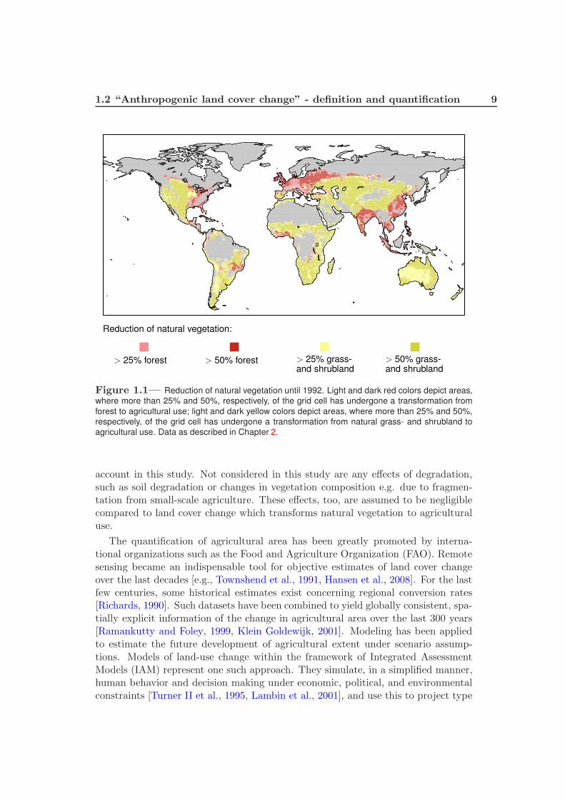
The present study focuses on ALCC as caused by the expansion or abandonmentof agricultural area, comprising cropland and pasture. This is the dominant typeof ALCC: At present, there exist about 15 million km2 of cropland and 34 millionkm2 of pasture [FAO, 2007, data for year 2003]. Both forests and natural grass- andshrublands are affected by the agricultural expansion — the regional distributionfor the early 1990s is shown in Fig. 1.1. Compared to the 49 million km2 of agricul-ture, urban areas currently cover only about 4 million km2 [Douglas, 1994]. Theycertainly exhibit a strong local influence on climate [e.g., Jin et al., 2005], but theirlarger contribution to global climate change must be expected via the food demandof a growing population, increasing the demand for agricultural areas [DeFries et al.,2004]. Forestry, on the other hand, is second-order to agriculture both in terms ofarea and emissions — wood harvest contributed on the order of 10% to land-usechange emissions over the last 150 years [Houghton, 1999]. As long as forest is usedin a sustainable way, loss of biomass is largely compensated by regrowth [Houghton,2003]. Part of the global wood demand is also covered by wood harvest on areassubsequently used for agriculture; such areas contribute to the ALCC taken into
1.2 “Anthropogenic land cover change” - definition and quantification 9
Reduction of natural vegetation:
> 25% forest > 50% forest > 25% grass-and shrubland
> 50% grass-and shrubland
Figure 1.1— Reduction of natural vegetation until 1992. Light and dark red colors depict areas,
where more than 25% and 50%, respectively, of the grid cell has undergone a transformation from
forest to agricultural use; light and dark yellow colors depict areas, where more than 25% and 50%,
respectively, of the grid cell has undergone a transformation from natural grass- and shrubland to
agricultural use. Data as described in Chapter 2.
account in this study. Not considered in this study are any effects of degradation,such as soil degradation or changes in vegetation composition e.g. due to fragmen-tation from small-scale agriculture. These effects, too, are assumed to be negligiblecompared to land cover change which transforms natural vegetation to agriculturaluse.
The quantification of agricultural area has been greatly promoted by interna-tional organizations such as the Food and Agriculture Organization (FAO). Remotesensing became an indispensable tool for objective estimates of land cover changeover the last decades [e.g., Townshend et al., 1991, Hansen et al., 2008]. For the lastfew centuries, some historical estimates exist concerning regional conversion rates[Richards, 1990]. Such datasets have been combined to yield globally consistent, spa-tially explicit information of the change in agricultural area over the last 300 years[Ramankutty and Foley, 1999, Klein Goldewijk, 2001]. Modeling has been appliedto estimate the future development of agricultural extent under scenario assump-tions. Models of land-use change within the framework of Integrated AssessmentModels (IAM) represent one such approach. They simulate, in a simplified manner,human behavior and decision making under economic, political, and environmentalconstraints [Turner II et al., 1995, Lambin et al., 2001], and use this to project type

10 1 INTRODUCTION
and extent of future agriculture. Modeling is also applied to assess the very begin-nings of agriculture. For example, there exist models that simulate the emergenceof agriculture depending on the geographical conditions of a region, and the sub-sequent spread of agricultural practices [Wirtz and Lemmen, 2003]. However, thetime period after the emergence of agriculture and prior to the last three centuriesposes a problem, since neither process-based simulation nor inference from statis-tical information is possible. Local, and mostly indirect, evidence for agriculturalextent for earlier times exists from archeology and historical records, but no globallyconsistent approach has yet quantified area and distribution of agriculture.
There exists thus a gap in our knowledge of global agricultural expansion, en-compassing the last several thousand years. This gap needs to be closed beforedetailed statements can be made concerning the past effects of ALCC on climate.Filling the gap for the last 1200 years is the topic of Chapter 2.
This chapter has been published in Global Biogeochemical Cycles [Pongratz et al.,2008b] (verbatim quote, but with references merged in the thesis bibliography; samefor the following Chapters), and in altered form in Reports on Earth System Science
[Pongratz et al., 2008a].
The historical context, in which the agricultural development of the last millen-nium must be seen, will be outlined in the following section.
1.3 A brief summary of the history of agriculture
Several theories have been proposed on how and why agriculture has developed.These theories include (1) the fortuitous invention and subsequent spread of theidea of cultivation or livestock farming due to apparent advantages; (2) a forcedchange to agriculture due to population pressure, reduced availability of wild food,or an environmental change at the Pleistocene-Holocene transition; (3) a coevolutionof domesticates, human management, and agricultural society, i.e. an unintendedselection of plants and animals in the habitat of man [Vasey, 1992, ch. 2],[Diamond,1999, ch. 6]. Though little more than protection of suitable plants was enough forcultivation in some cases, [Grigg, 1974, ch. 2] agriculture was most often associ-ated with the process of domestication, i.e. a change in morphology by selectionunder human management towards favorable features. Such features may be largeredible parts than wild forms, less shattering or dropping of fruits and seeds aftermaturation, and outcompeting wild forms on managed land [Vasey, 1992, ch. 2].Domestication greatly increased yields, probably by a factor of 2–3, e.g. for cerealsduring the first thousand years following the Neolithic Revolution [Gepts, 2004]. Inparallel, management methods evolved that intensified the cultivation, leading to anoverall increase of the nutritional density of land. As a consequence, an agriculturalsystem could upkeep population densities a factor 10–100 higher than in hunting and
1.3 A brief summary of the history of agriculture 11
gathering societies [Diamond, 1999, ch. 4]. Surpluses of food could be created andin combination with a sedentary lifestyle facilitated the formation of stratified soci-eties, in which large numbers of people are supported by few farmers. As suggestede.g. by Diamond [1999, ch. 13], agriculture may therefore have been the trigger formany of the features of modern societies, allowing for rapid development of technol-ogy. Agriculture proved to be advantageous over the hunting and gathering lifestylein many regions and was frequently adopted by neighboring hunters and gatherers.Agricultural people with their high population growth and advanced technologiesalso simply replaced or destroyed non-farming societies — all with the consequencethat agriculture became the by far dominating lifestyle over hunting and gathering.
The “invention” of this new lifestyle happened at only few independent loca-tions. The most certain origins of agriculture lie in the Fertile Crescent (around8500 B.C), North China (by 7500 B.C), southern Mexico (by 3500 B.C.), and coastalPeru (around 3000 B.C.) [Diamond, 1999, ch. 5]. All these places hold evidence ofcereal domestication and are thus the founders of “seed agriculture” [Grigg, 1974,ch. 2]. Several other regions are possible candidates for an independent developmentof agriculture. In particular regions of tropical “vegeculture”, which relies mainlyon root crops, may also have taken the step to agriculture independently, e.g. Ama-zonia and tropical West Africa. From these centers of origin, agriculture spread.The spread may have taken place in the form of the domesticated plant or animal,of the farmers themselves and their knowledge, or of only the idea of agriculture[Grigg, 1974, ch. 2]. The spread of agricultural systems was still continuing duringthe last millennium, the period covered in this study, including the Bantu expansionon the African continent, the European settlement of Australia, and the exchangeof plants between the New and the Old World. On the other hand, Europe andthe Mediterranean, Southwest, South and Southeast Asia, and several other regionshave been reached by the spread of agricultural systems already millennia earlier.Here, it is not the advent, but the expansion of agricultural area that changes theland cover. All these developments are described in more detail in Chapter 2. A spe-cial focus is laid on the links between population and agricultural areas. As statedbefore, the onset of agriculture as well as the refinement of techniques may havebeen triggered by population pressure; and they allowed for population growth byincreasing the nutritional density of land. Population number and agricultural areaare further immediately linked during times where the development of new agrarianmethods was slow; then, dietary requirements of a person under a given nutritionaldensity determine the areas of cropland and pasture in a region as a function of itspopulation number. This connection has been employed to reconstruct agriculturalextent for the preindustrial period of the last millennium. It would be futile, how-ever, to apply this argument to the recent development of agriculture. Technologydeveloped during industrial times, e.g. artificial fertilizers, mechanization and thebroad application of fuel-driven machines, and systemized breeding up to geneticallymodified plants have again multiplied nutritional density [Vasey, 1992, ch. 10].
12 1 INTRODUCTION
1.4 The last millennium
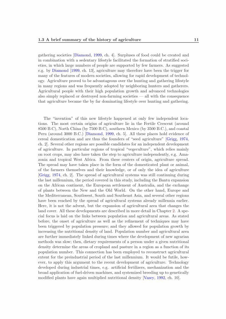
Immanent in the expansion of agriculture was an increasing modification of theEarth’s land surface. Especially seed agriculture needs complete clearing of thenatural vegetation, and vegeculture was often implemented in a system of shiftingcultivation, meaning that forest was burnt down. This modification of the land sur-face must have been particularly strong during the last millennium: Between AD 800and the early 18th century the world’s population tripled to one billion people, whileit had remained at below 220 million for the preceding millennia (Fig. 1.2). The lastmillennium must therefore have been associated with an agricultural expansion atunprecedented pace. This makes it particularly appropriate for studies on preindus-trial human impact — if no significant impact from ALCC can be determined forthis period, an anthropogenic signal is unlikely to be detectable for earlier millennia.
The last millennium is particularly suitable for ALCC-climate studies for two fur-ther reasons: First, ALCC was the dominating anthropogenic perturbation up untilthe 20th century — only after the 1930–50s, CO2 emissions from fossil-fuel com-bustion grew substantially larger than ALCC emissions [Houghton, 2008, Marlandet al., 2008], and prior to the industrialization ALCC was the only anthropogenicdisturbance. The preindustrial period allows an analysis of the ALCC impact un-affected of other human activity. Second, the last millennium represents one of thebest-documented periods of climate change on a multi-century timescale. Climateproxies such as ice core records and tree rings give detailed insight into the evolu-tion of temperature and CO2. Once all known natural and anthropogenic forcingshave been isolated in their effect on climate, their combined impact can be validatedagainst such climate reconstructions.
With its focus on preindustrial ALCC and climate, parts of this work evaluatewith more detailed methods aspects of previous studies. Two challenging hypothesesare the possible early impact of humans on atmospheric CO2, and the possiblecontribution of ALCC to the “Little Ice Age”:
A scientific dispute has been started with the “early anthropogenic hypothesis”by Ruddiman [2003, 2007]. Ruddiman concludes that the rise in atmospheric CO2
reconstructed from ice core data for the last few millennia is anomalous as comparedto what should be expected from its natural evolution in analogy to previous glacialand interglacial cycles. The beginning of the anomalous rise in CO2 coincides withthe beginning of agricultural activity about 8000 years ago. This anomaly, summingto 40 ppm by the end of the preindustrial period, can be explained at least in part byALCC, according to his hypothesis. In addition, temporal variability of global CO2
may be caused by historic events that cause regional abandonments of agriculturalarea, e.g. epidemics and warfare associated with a large reduction in population.The hypothesis extends further to a similarly anomalous rise in CH4, which mayalso be attributable to human action. Subsequent studies by other groups haveinvestigated aspects of this work and come to different conclusions, ranging from asubstantially smaller contribution of human activity to the anomaly than suggested
1.4 The last millennium 13
0
1
2
3
4
5
6
7
-10000 -8000 -6000 -4000 -2000 0 2000
bill
ion
pe
op
le
year
0.0
0.4
0.8
1.2
1.6
800 1000 1200 1400 1600 1800
AsiaEuropeAfricaLatin AmericaNorth AmericaOceania
Figure 1.2— The world’s population 10,000 B.C. to AD 2000. Data from Clark [1967], McEvedy
and Jones [1978].
[Olofsson and Hickler, 2008] to negligible human influence [Joos et al., 2004]. Naturalprocesses have been put forward to explain the evolution of CO2 over the Holoceneand scrutinized the estimate of the natural trend [e.g., Claussen et al., 2005]. Noconsensus, however, has been found. Even if it was not several millennia into thepast that may have been affected by ALCC-induced emissions, it has been notedthat a high CO2 concentration as far back as the early 1800s precludes large-scalefossil-fuel combustion as the only substantial contribution to changes in atmosphericcomposition [e.g., Kammen and Marino, 1993]. The CO2 aspects of this hypothesiswill be reassessed in Chapter 4 of this thesis, with a combination of data and methodsthat goes beyond any of the mentioned studies and allows a novel level of detail inthe analysis.
The beginning of the last millennium is termed the “Medieval Warm Epoch” forat least some regions, like western Europe, which experienced relatively high tem-peratures during that time [Lamb, 1965]. Following the 14th century, a long-termcooling set in on the Northern Hemisphere leading to the so-called “Little Ice Age”[Mann and Bradley, 1999]. Various reconstructions of Northern Hemisphere temper-ature show a considerable range for timing and strength of the cooling, but all agreein a general downward trend between the medieval times and the 16th–19th century[Osborn and Briffa, 2006, Jansen et al., 2007]. In the reconstruction by Mann andBradley [1999], for example, temperatures at the end of the preindustrial periodwere about 0.2 K lower than at the beginning of the millennium. This cooling hasbeen thought to be possibly related to astronomical forcing which may have induceda long-term downward trend in global temperature since the mid-Holocene at anaverage rate of −0.01 to −0.04 K/century [see Berger, 1988, Mann and Bradley,

14 1 INTRODUCTION
1999]. Recent modeling studies, however, suggest that the orbital forcing may in-deed induce noticeable changes in the monthly response, but has only negligibleinfluence on the annual temperature response in the Northern Hemisphere over thelast millennium [Bauer and Claussen, 2006]. Further possible contributions to thecooling may come from century-scale variations in solar irradiance [Mann et al.,1998]. Another hypothesis, however, assumes ALCC as driving force behind theNorthern Hemisphere cooling. In a study on Europe, Goosse et al. [2006] simulatea cooling of 0.4–0.5 K during the past millennium until today due to changes in thephysical properties of the land surface by ALCC. This notion is supported by othermodeling studies that find a Northern Hemisphere cooling of 0.35 K over the pastmillennium [Bauer et al., 2003], 0.25 K AD 1000–1900 [Govindasamy et al., 2001],and global cooling of 0.13–0.25 K [Brovkin et al., 2006]. All of these studies haveapplied ad-hoc approximations of preindustrial ALCC. However, assessing regionaleffects of ALCC for specific time periods needs detailed knowledge concerning theevolution of the climate forcing. Chapters 2, 3, and 5 quantify this forcing and itspossible climatic influence.
1.5 Biosphere-atmosphere interactions and goals of thisstudy
Preliminary remark on the methodology. As will become clear in the follow-ing Chapters, this thesis relies on modeling to assess the effects of ALCC on climateand the carbon cycle. Climate modeling is a valuable tool in particular for theoreti-cal studies, e.g. to assess the climate response to only a subset of climate forcings asdone in this study for ALCC only, or for an estimate of quantities that are not di-rectly observable. In this thesis, the interaction of the biosphere with the other partsof the climate system are simulated using a complex Earth system model: Climateis simulated by a climate model comprising an atmosphere/ocean general circula-tion model (AOGCM), which consists of an atmosphere model (ECHAM5, Roeckneret al. [2003]) and an ocean and sea ice model (MPI-OM, Marsland et al. [2003]).Coupled to the ocean is an ocean biogeochemistry model (HAMOCC5, Wetzel et al.[2005]). Coupled to the atmosphere is a modular land surface scheme (JSBACH,Raddatz et al. [2007]). The human dimension is integrated into the model by pre-scribing changing maps of land cover as boundary condition to the atmosphere.The setup of the model is chosen according to the respective question, e.g., eitherequilibrium or transient studies are chosen, and all or only parts of the four modelcomponents may be included. In some cases, the original model code is adapted orextended to answer a particular question. All interactions of the biosphere with theother components of the climate system that are described in detail in the followingcan be simulated by this Earth system model.
Radiative forcing from albedo changes. The biosphere and atmosphere inter-act via a multitude of mechanisms, which can all be altered by ALCC. Generally,
1.5 Biosphere-atmosphere interactions and goals of this study 15
two groups of mechanisms are distinguished, biogeophysical and biogeochemical ones[Claussen, 2004]. Biogeophysical mechanisms describe the influence on climate bythe modification of the physical properties of the land surface such as albedo, rough-ness, and evapotranspiration. Both morphological and physiological properties ofthe vegetation cover are therefore important for the biosphere-atmosphere fluxes ofenergy, momentum, and substances like water. An immediate impact on the energybalance is induced by albedo changes. Albedo, the “reflectivity” of the land surface,usually increases with ALCC that implies deforestation, due to the higher snow-freealbedo of non-forest vegetation and the snow masking effect of forest [Bonan et al.,1992]. The difference is particularly large during the winter and spring season forthose areas with snow cover, where albedo may change from 0.2 for forest to 0.8on an open field [Robinson and Kukla, 1984]. Only in cases with dark underlyingsoil albedo may decrease, when the vegetation cover is sparser under agriculturaluse. An increase in albedo decreases the absorption of solar radiation and therebyreduces turbulent heat fluxes [Pitman et al., 2004]. A decrease in the latent heatflux may decrease the water vapor content in the boundary layer, while holding backwater in the soil or increasing runoff. A decrease in the sensible heat flux may re-duce the heating of the boundary layer. Both may decrease cloud cover (a potentialnegative feedback on net radiation by decreasing planetary albedo) and convection[Bonan, 2002]. The reduction in absorbed solar radiation and heat fluxes also hasconsequences on surface temperature. Modeling studies suggest that through thesebiogeophysical effects ALCC at mid- and high latitudes induces cooling [e.g., Bonanet al., 1992, Claussen et al., 2001, Bounoua et al., 2002].
A common measure to quantify the biogeophysical implications of ALCC is ra-diative forcing (RF). RF, in W/m2, is a convenient first-order measure of the im-portance of a perturbation in causing climate change. It is defined as the radiativeflux change of the tropopause after the stratospheric temperature has come to aradiative equilibrium, but prior to any feedbacks [e.g., Hansen et al., 1997]. It isconvenient because the RF, ∆F can be related to the change in global mean surfacetemperature, ∆T , in a simple linear equation:
∆T = λ · ∆F . (1.1)
The climate sensitivity parameter λ is usually determined for each model from theequilibrium change of global mean surface temperature in a simulation forced by2·CO2. Typical values of λ lie in the range of 0.5–1.1 K/(W/m2) [Meehl et al., 2007].Two advantages of the RF measure are: (1) It is computationally less expensivethan the full climate response. For greenhouse gases, for example, it implies onlya double-calculation of the radiative transfer scheme in the same climate. (2) RFis less model-dependent than the climate response: Questions like “what are theconsequences of a doubling of CO2?” result in very different answers from differentmodels. The reason for this lies in different parameterizations of important feedbackslike changes in water vapor, cloud properties, sea ice and snow extent. Excludingany feedbacks, the RF implies a smaller uncertainty than the climate response. Ittherefore allows one to more objectively compare perturbations of different nature in

16 1 INTRODUCTION
their climatic importance. The RF measure has been successfully applied to classicclimate perturbations such as well-mixed greenhouse gases and solar variability. Ithas also become the standard tool to compare the importance of ALCC to otherperturbations, despite known shortcomings in this application (see Sec. 3.1). Withrespect to ALCC, RF is used as a predictor of the climate response towards allbiogeophysical effects of ALCC, although it is determined only for the changes insurface albedo.
In Chapter 3 the RF measure is applied to ALCC for the entire last millennium,with the following objectives:
1. To give a measure of the climatic importance of preindustrial ALCC that canbe compared consistently to estimates of the last two to three centuries, forwhich there exist studies.
2. To compare the importance of preindustrial ALCC to concurrent, natural cli-mate perturbations such as volcanic eruptions and solar variability.
These two first items give a first-order answer to the question of whether ALCCcould indeed have significantly altered preindustrial global or hemispheric meantemperature and be responsible for the Northern Hemisphere cooling.
With the help of the high-detail ALCC reconstruction from Chapter 2, new in-sight is gained in the regional distribution of the anthropogenic climate perturbationand the temporal evolution over the preindustrial period. This allows
3. To indicate “hot spots” of the perturbation of the energy balance a millenniumago and their change through history. As mentioned above, the agriculturalcenters shifted regionally with time, which prohibits us to infer the historyfrom the present state.
4. To follow the change of forcing pattern over history and to assess the effectsof historic events on the energy balance.
This chapter has been published in Geophysical Research Letters [Pongratz et al.,2009].
Biogeochemical effects of anthropogenic land cover change. In addition tothe biogeophysical mechanisms, the biosphere interacts with atmosphere and oceanvia various biogeochemical cycles. Biogeochemical mechanisms of ALCC involvethe emissions of methane (CH4) [e.g., Hein et al., 1997], emission of aerosols frombiomass burning and dust [e.g., Andreae and Merlet, 2001], and influence on nutri-ent cycles such as nitrogen, iron, and phosphorus cycles [e.g., Galloway et al., 1995,Denman et al., 2007]. Plants further interact with the carbon cycle via the emissions
1.5 Biosphere-atmosphere interactions and goals of this study 17
of biogenic volatile organic compounds (BVOCs), reactive carbon compounds thataffect aerosol formation and atmospheric chemistry, influencing e.g. ozone concen-tration [Fehsenfeld et al., 1992, Andreae and Crutzen, 1997].
The most important biogeochemical effect, however, through which the biosphereinfluences present climate change, is the altered exchange of CO2 with the atmo-sphere [Denman et al., 2007]. By altering the atmospheric concentration of thegreenhouse gas CO2, ALCC modifies the Earth’s energy balance and thus climate.On the one hand, the CO2 flux from the biosphere to the atmosphere is increasedby ALCC, mostly caused by a loss of terrestrial biomass. About one third of theanthropogenic CO2 emissions over the last 150 years are the direct result of ALCC[Houghton, 2003]. Counteracting the emissions, on the other hand, is an enhanceduptake of CO2 during photosynthesis by both natural and agricultural vegetation.The underlying increase in productivity is presumably caused, among other factors,by CO2 fertilization: Experimental studies of the physiological response of plants toincreased ambient CO2 indicate increased photosynthetic rates and reduced stom-atal conductance. This effect is larger for plants with a C3 photosynthetic pathway(trees and the majority of mid- and high-latitudinal herbaceous plants) than forthose with a C4 photosynthetic pathway (tropical herbaceous plants) [e.g., Bazzaz,1990].
The net effect is that the terrestrial biosphere has turned from a source to asink during the recent decades; quantifications of the individual fluxes have beencited in Sec. 1.1. This quantification is crucial for understanding past and presentclimate change, and for potentially mitigating future changes, but still involves largeuncertainties (see Sec. 4.1). Considering the long lifetime of atmospheric CO2, it isfurther important to cover the long history over which the perturbation of carbonfluxes may have accumulated. Last but not least, it is crucial to take into accountthat the biosphere is just one of three interacting compartments; the coupling ofocean, atmosphere, and biosphere needs to be taken into account to assess theinfluence of ALCC on the global carbon cycle.
In Chapter 4 the effects of ALCC on the carbon cycle are assessed in detail incoupled model simulations, with the following main goals:
1. To assess the historical effects of ALCC on temperature and the carbon cyclein an isolated form, i.e. isolated from other forcings. This requires an idealizedmodeling study, in which only ALCC is allowed to change.
2. To quantify both source and sink terms of carbon: An estimate will be givenfor primary CO2 emissions from ALCC, which are not known in high temporalresolution prior to AD 1850. In addition to carbon emissions, uptake in theocean as well as by biospheric restorage will be quantified spatially for differenteras. This leads to estimates of how much ALCC mitigated its own carbonsignal in different time periods.
3. To determine the beginning of significant human influence on the individual
18 1 INTRODUCTION
carbon pools, including atmospheric CO2. Thus, Ruddiman’s hypothesis ofthe early anthropogenic impact will be assessed. The setup of the simulationsallows such an assessment at unprecedented detail.
4. To determine whether historic events could indeed have been responsible fordrops in CO2 as reconstructed from ice core records, and if not, which processesinhibit a detectable signal. The medieval Black Death in Europe, the Mongolinvasion, and the fall of the Ming Dynasty in China will be assessed.
This chapter has been submitted to Global Biogeochemical Cycles [Pongratz et al.,submitted].
Biogeophysical effects of anthropogenic land cover change. The previouspart focuses on the carbon cycle, but the simulations performed include the biogeo-physical mechanisms in addition to the biogeochemical mechanisms. Temperatureand turbulent heat fluxes may be altered by the increase in albedo, as explainedabove. But further biogeophysical processes are at work in the coupled system:First, ALCC alters roughness length. Surface roughness length is a measure for thedrag force that the land surface exerts on the the lowest layer of the atmosphere;the aerodynamic resistance impeding the transfer of momentum and scalar proper-ties such as heat, water vapor, and CO2 depends inversely on the roughness length.Deforestation usually reduces roughness length, resulting in higher aerodynamic re-sistances and smaller fluxes for otherwise identical conditions [e.g., Bounoua et al.,2002, Pitman et al., 2004]. Second, fluxes of water are also directly influenced byvegetation as it controls the availability of water for evapotranspiration. ALCC al-ters the photosynthetic activity on leaf and canopy level, e.g. by a change of thephotosynthetic pathway between C3 and C4 or a change in phenology and leaf areaindex. Coupled to the photosynthetic activity are the stomatal and canopy con-ductances, which control the transpiration of the plant and canopy. ALCC maytherefore alter the amount of water transpired, and influences thereby soil moisture,runoff, and the partitioning of energy into latent and sensible heat fluxes. Via stom-atal conductance and photosynthesis, the fluxes of carbon and water through theplants are coupled [e.g., Sellers et al., 1992]. As indicated in Sec. 1.1, via reducedevapotranspiration ALCC may lead to a warming counteracting the cooling effectof albedo changes, which may regionally add to a net warming or cooling effect.
In Chapter 5 the climate change from the biogeophysical mechanisms of ALCCis quantified on regional and global scale for the last millennium. The samemethods and data are applied as in Chapter 4; this implies not only an analysis ofthe biogeophysical effects of historical ALCC at unprecedented detail, but it alsoallows a consistent comparison of the strength of biogeophysical and biogeochemicaleffects in their influence on climate and the carbon cycle. This chapter presents

1.5 Biosphere-atmosphere interactions and goals of this study 19
new results for the biogeophysical aspects of historical ALCC, but is also a synopsisof the previous parts of this thesis with the following goals:
1. The strength of the climatic response to biogeophysical mechanisms will becompared to that of biogeochemical mechanisms for past and present, therebyanswering the question whether global mean temperatures have been domi-nated by biogeophysical or biogeochemical effects of ALCC. A spatially explicitanalysis identifies strength and sign of regional contributions to the global sig-nal. The biogeophysical response of the model is analyzed and compared toother models.
2. A substantial influence of ALCC on carbon source and sink terms has beenfound in Chapter 4. Here, the question is answered whether biogeophysicaleffects of ALCC contribute to the disturbance of carbon pools.
3. Two forcings of ALCC have been quantified: RF from albedo changes in Chap-ter 3, and CO2 emissions in Chapter 4. Their counteracting strength is assessedand compared to the temperature responses to biogeophysical and biogeochem-ical mechanisms. The question is answered whether the forcings are a goodindicator for the individual and overall temperature responses.
4. As outlined in Sec. 1.1 ALCC features prominently as tool for climate changemitigation. Considering that different mechanisms are counteracting eachother it is not clear whether ALCC in a specific geographical location re-sults in a cooling or warming contribution to global climate change. The netradiative contribution of ALCC to global climate change will be quantified ina geographically explicit form, indicating whether a local reversion of ALCCcould mitigate climate change.
Parts of this chapter are in preparation for submission to Geophysical Research
Letters.

21
Chapter 2
A Reconstruction of GlobalAgricultural Areas and LandCover for the Last Millennium
Abstract
Humans have substantially modified the Earth’s land cover, especially by transform-ing natural ecosystems to agricultural areas. In preindustrial times, the expansionof agriculture was probably the dominant process by which humankind altered theEarth system, but little is known about its extent, timing, and spatial pattern. Thisstudy presents an approach to reconstruct spatially explicit changes in global agricul-tural areas (cropland and pasture) and the resulting changes in land cover over thelast millennium. The reconstruction is based on published maps of agricultural areasfor the last three centuries. For earlier times, a country-based method is developedthat uses population data as a proxy for agricultural activity. With this approach,the extent of cropland and pasture is consistently estimated since AD 800. Theresulting reconstruction of agricultural areas is combined with a map of potentialvegetation to estimate the resulting historical changes in land cover. Uncertaintiesassociated with this approach, in particular owing to technological progress in agri-culture and uncertainties in population estimates, are quantified. About 5 millionkm2 of natural vegetation are found to be transformed to agriculture between AD800 and 1700, slightly more to cropland (mainly at the expense of forested area)than to pasture (mainly at the expense of natural grasslands). Historical eventssuch as Black Death in Europe lead to considerable dynamics in land cover changeon regional scale. The reconstruction can be used with global climate and ecosystemmodels to assess the impact of human activities on the Earth system in preindustrialtimes.
22 2 MILLENNIUM LAND COVER RECONSTRUCTION
2.1 Introduction
One of the most striking impacts of humankind on its environment is the transfor-mation of natural ecosystems to managed areas. At present, 30–50% of the Earth’sland cover have been substantially modified by human land use, primarily by theexpansion of agriculture [Vitousek et al., 1997]. By 2003, about 15 million km2
of cropland and 34 million km2 of pasture have replaced natural land cover [FAO,2007], providing much of the ecosystem goods and services humanity has becomedependent on. Such large-scale modifications of the land surface can have importantconsequences for the Earth system, most notably through their impact on ecologicalfunctioning, and the biogeophysical and biogeochemical interactions with the atmo-sphere. Significant changes in structure and functioning of ecosystems and a lossof biodiversity have already been attributed to human interference [UNEP, 1995,Haberl et al., 2007]. Energy balance and hydrological cycle are significantly affectedby present-day land use activity [Betts, 2001, Davin et al., 2007], and global carbonand nitrogen cycles have been altered severely [Galloway et al., 1995, Denman et al.,2007]. For example, about 35% of anthropogenic CO2 emissions during the last 150years resulted directly from land use [Houghton, 2003], making it one of the keyagents of anthropogenic climate change. Recognition of land use as a possible wayto mitigate climate change and the increasing concern of the scientific communityabout the availability of natural resources has further brought the consequencesof human-induced land cover change to public awareness [Millennium EcosystemAssessment, 2005, Barker et al., 2007].
Given the growing evidence of the impact anthropogenic land cover change ex-erts on the Earth system, it is not surprising that today much effort is put intoquantifying these changes. In recent years, remote sensing offers a valuable tool formonitoring land cover change [Townshend et al., 1991, Brown de Colstoun et al.,2006]. Historical data of agricultural activity allow rather solid estimates for the last300 years [Ramankutty and Foley, 1999, Klein Goldewijk, 2001]. By contrast, quan-tifications of global land cover change prior to AD 1700 are scarce, although it is wellknown that humans have actively managed and transformed the world’s landscapesalready for millennia [Grigg, 1974]. It is also recognized that these preindustrial landcover changes may have significantly contributed to the variability of atmosphericcomposition observed from ice core records [DeFries et al., 1999, Ruddiman, 2007].Yet, the strength of human impact is still highly controversial [Joos et al., 2004].Much of the dispute is centered around the lack of knowledge concerning extent,timing, and spatial pattern of historical land cover change. Those studies that haveso far accounted for anthropogenic land cover change in preindustrial times in globaland regional Earth system studies used the simplification to either keep land coverfixed prior to the 18th century (e.g. Stendel et al. [2006], Tett et al. [2007]) or tolinearly interpolate between potential vegetation in AD 1000 and the state of landcover of AD 1700 (e.g. Brovkin et al. [1999], Goosse et al. [2006]). Both approaches,however, entirely disregard any detail of human history.
In this study, we present the first detailed reconstruction of global agricultural
2.2 Step 1: Adaptation of agricultural data since AD 1700 23
areas (cropland and pasture) and the resulting changes in land cover over the lastmillennium. Special emphasis is placed on the preindustrial period, as it has notbeen subject of consistent analysis before. In the time period between AD 800 andthe early 18th century, the world’s population tripled [McEvedy and Jones, 1978].As more people required more food and commodities from agriculture and naturalresources, this period must have been associated with agricultural expansion at anunprecedented pace [Grigg, 1974, Richards, 1990]. As reliable data on historical agri-cultural areas is sparse, we develop a simple method for its reconstruction based onpopulation estimates. Agriculture is inherently linked to population [Vasey, 1992],which allows us to use country-based estimates of historical population as proxy foragricultural areas. With this method, the cropland and pasture maps of Ramankuttyand Foley [1999] and Foley et al. [2003] at 0.5 degree resolution for the last 300 yearsare extended back into the past to give consistent estimates of cropland and pasturesince AD 800 on a geographically explicit basis. This “millennium reconstruction”of agricultural areas is combined with a map of potential vegetation to also estimatehistorical changes in land cover.
The reconstruction of agricultural areas is restricted to cropland and pasture.For cropland, the definition of “arable and permanent crops” from the Food andAgricultural Organization (FAO) is adopted, which includes land under temporaryand permanent crops, temporary meadows for mowing or pasture, land under mar-ket and kitchen gardens, and land lying temporarily fallow. The abandoned landresulting from shifting cultivation is not included. For pasture, the FAO category“permanent pasture” is used. It includes all land used permanently for herbaceousforage crops, either cultivated or growing wild.
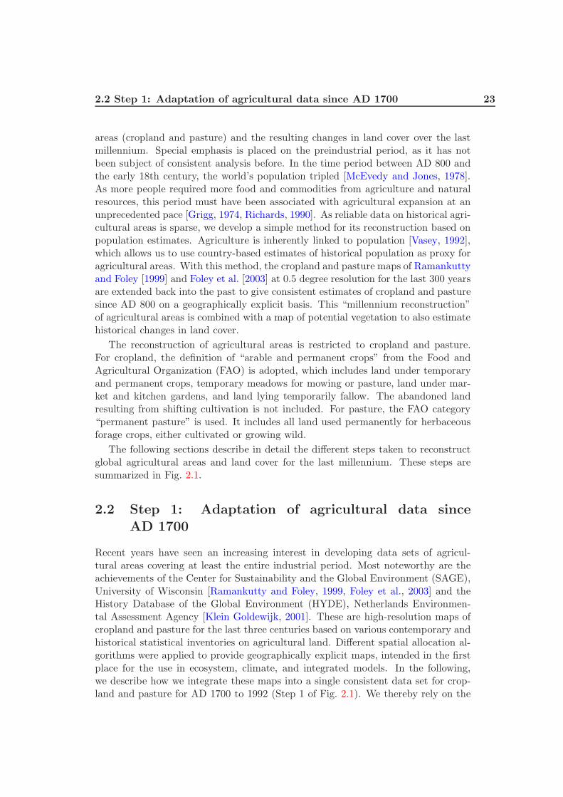
The following sections describe in detail the different steps taken to reconstructglobal agricultural areas and land cover for the last millennium. These steps aresummarized in Fig. 2.1.
2.2 Step 1: Adaptation of agricultural data since
AD 1700
Recent years have seen an increasing interest in developing data sets of agricul-tural areas covering at least the entire industrial period. Most noteworthy are theachievements of the Center for Sustainability and the Global Environment (SAGE),University of Wisconsin [Ramankutty and Foley, 1999, Foley et al., 2003] and theHistory Database of the Global Environment (HYDE), Netherlands Environmen-tal Assessment Agency [Klein Goldewijk, 2001]. These are high-resolution maps ofcropland and pasture for the last three centuries based on various contemporary andhistorical statistical inventories on agricultural land. Different spatial allocation al-gorithms were applied to provide geographically explicit maps, intended in the firstplace for the use in ecosystem, climate, and integrated models. In the following,we describe how we integrate these maps into a single consistent data set for crop-land and pasture for AD 1700 to 1992 (Step 1 of Fig. 2.1). We thereby rely on the
24 2 MILLENNIUM LAND COVER RECONSTRUCTION
SAGE fractional cropland
1700-1992
Revised fractional cropland
1700-1992
Regional sums
from HYDE
pasture
1700-1992
Ste
p 1
: Ag
ricu
ltura
l are
as
AD
17
00
-19
92
Regional
modifications
Regional
modifications
SAGE fractional pasture
1992
Fractional pasture
1700-1992
(Sub-)National population
800-1700
Fractional cropland
800-1700
Ste
p 2
: Ag
ricu
ltura
l
are
as
AD
80
0-1
70
0
1700
Regional modifications
Fractional pasture
800-1700
1700
Fractional potential
vegetation map
SAGE 5min potential
vegetation map
Spatial aggregation
Reclassification
Reconstruction of agricultural areas 800-1992
Land cover reconstruction 800-1992
Ste
p 3
: La
nd
co
ve
r
AD
80
0-1
99
2
Figure 2.1— Scheme for reconstructing agricultural areas and land cover AD 800 to 1992.
Double arrows indicate linear backscaling.
SAGE data where possible as its fractional character supplies additional sub-gridinformation.
2.2.1 Cropland
Ramankutty and Foley [1999] developed a simple algorithm to link present remotesensing data and historical cropland inventories. Inventory data was compiled onthe level of today’s political units (subnational data for some of the largest coun-tries) and is based on data published by the Food and Agricultural Organization(FAOSTAT) for 1961-1992 and a variety of sources for earlier times, most notablyestimates from Houghton and Hackler [1995] and Richards [1990]. We use their timeseries AD 1700 to 1992 of global croplands for the millennium reconstruction, butapply some revisions. First, we replace the West Africa region by the improvedregional data set of Ramankutty [2004], which we extend to previous years using
2.3 Step 2: Reconstruction of agricultural areas AD 800 to 1700 25
population trends [Klein Goldewijk, 2001]. We apply some further corrections ofthe cropland pattern in the 18th and 19th century for specific regions to bettermatch historical evidence. They were necessary in order to provide suitable mapsas starting point for the reconstruction of earlier centuries. In particular, the lackof subnational data in the Former Soviet Union (FSU) led to maintenance of the1992 crop pattern and to significant crop area in Siberia in historical times. We re-distribute total crop area using subnational population data derived from McEvedyand Jones [1978] and United Nations Statistics Division [2006]. In a similar way,the crop pattern of Australia and New Zealand are adjusted to reflect the history ofEuropean immigration (for details see Pongratz et al. [2008a]).
2.2.2 Pasture
For global pastures, where SAGE provides only a single map for 1992, we extend thisdata to a time series AD 1700 to 1992. First, we calculate regional totals of pasturearea for each year from the 1992 areas and rates of change from Klein Goldewijk[2001]. Calculations are performed on country level after 1960 and for the 10 regionsdefined by Houghton et al. [1983] prior to 1960 adapting the same regional break-down as has been used for the temporal information of HYDE. For each year, thepasture totals are then distributed spatially within each country or region. While themethod of Ramankutty and Foley [1999] to extend the 1992 map of cropland backinto the past was to generally maintain the 1992 pattern of cropland throughouttime (i.e. the grid cells within a country keep their cropland fractions in the sameproportion relative to each other, while the total area changes with time), we chosea different method for pasture. The pasture area is thereby distributed around theexisting cropland in a way that not the pattern of pasture, but of total agriculturalarea (cropland plus pasture) is maintained throughout time. The advantage of thismethod is that it allows to take into account the expansion of crop on pasture areathat has been observed in the past [Grigg, 1974]. The modifications applied to thecrop time series concerning Australasia are also applied to the pasture time series.The modifications concerning the FSU are unnecessary as the pasture areas here areconnected to the extensive areas of traditional nomadic pastoralism of Kazakhstanand Mongolia [Kerven et al., 2006].
2.3 Step 2: Reconstruction of agricultural areas AD 800to 1700
Statistical databases built by international organizations and, more recently, remotesensing provide us with data and methods to consistently measure agricultural areasand land cover change of the last decades. Great efforts have been undertaken toextend this data back into the past; most notable with respect to its global coverageis the work by Houghton [1999], who compiled a multitude of regional studies relatedto historical land cover, and the data compilation by Richards [1990], which are basis
26 2 MILLENNIUM LAND COVER RECONSTRUCTION
also of the SAGE and HYDE studies. However, sources which address more thanthe local level become scarce when going back in time and rarely go beyond AD1650. Thus, we search for a proxy for agricultural area for which historical data ismore readily available on global scale.
We therefore utilize in this study the fact that agriculture is inherently linked topopulation. Prior to the 19th century, technology played a minor role in resourceextraction, and transportation was a limiting factor in preindustrial times for tradinglarge quantities of agricultural input and output over long distances [Vasey, 1992].Even if most societies had outgrown individual subsistence farming, autonomy forbasic needs still had to be largely realized on a regional level [Allen, 2000]. It istherefore appropriate to assume that agriculture occurred where people had settled,and the amount of land under human use is likely well correlated to the number ofpeople who had to be nourished. For this reason, we use population estimates asproxy for agricultural areas. Information on historical population numbers are muchmore readily available than on land cover; our main source of population data forAD 800–1700 is the Atlas of World Population History by McEvedy and Jones [1978],with regional modifications for Central and South America based on Clark [1967].McEvedy and Jones provide totals for most of today’s countries from 400 BC toAD 1975 based on a multitude of publications and support their estimates with shortessays stressing among others the role of agriculture. Where only data for largerregions is provided, we break the historical numbers down to country level using theHYDE population density map of AD 1700, assuming that the national proportionswithin a region remain constant. For some regions, sub-national data was used,especially for the FSU and Central and South America. In the latter region, nationalnumbers are broken down to better represent the spatial heterogeneity between thehigh cultures, with a significantly higher population density, and other tribes inpre-Columbian times (for details see Pongratz et al. [2008a]).
Population numbers are then translated for each country into estimates of cropand pasture area. In the absence of further information, it seems inappropriate touse anything more than the simplest assumptions. Thus, our basic assumption isthat in each country the ratio of area used per capita for crop and pasture did notchange prior to AD 1700. This ratio — the inverse of the nutritional density —is calculated for AD 1700 from the earliest agricultural map of the 300-years seriesdescribed in Sec. 2.2 and our population database. Today’s political borders, witha few subnational divisions where necessary, were chosen in order to be consistentwith the scale of Ramankutty and Foley [1999] and to allow for easy comparisonwith today’s statistical data. Using population as proxy for agricultural areas isnot a new approach; it has been suggested e.g. by Ramankutty et al. [2006] andhas been applied to more recent times by Houghton [1999]. Possible errors resultingfrom this method will be discussed in Sec. 2.5.
In order to convert national totals of crop and pasture area to geographically ex-plicit information, we make a second basic assumption: The pattern of agriculturalareas that we observe in each country in AD 1700 (Figs. 2.2 and 2.3) is similar toearlier spatial patterns. The persistence of the agricultural pattern in each coun-
2.3 Step 2: Reconstruction of agricultural areas AD 800 to 1700 27
try through time is a basic assumption in claiming only that the relative intensityof agricultural use within one country does not change between pixels. In otherwords, this generally means that suitable areas are cultivated more intensively thanless suitable ones within a country, independently of total cultivated area. Thesupra-national pattern, however, is reconstructed independently each year from thepopulation-based national estimates of agricultural areas. Within the accuracy ofthe AD 1700 global pattern, the relative importance between countries is therebycorrectly represented in earlier times. While human migrations across political bor-ders are implicitly taken into account by using country-based population data, theshift of settlement and cultivation pattern within the countries of the Americas afterthe European conquest is explicitly corrected for (see below).
The existing time series is scaled back in time, combining the above stated keyassumptions with the agricultural areas and population numbers of AD 1700 onnational level (step 2 of Fig. 2.1): The total area of agriculture of a country —cropland and pasture are each treated separately — is calculated for each yearfrom the agricultural area per capita and historical population. The pattern ofAD 1700 determines the relative fractions of the agricultural area of the pixels withina country. In countries where agricultural area in earlier years exceeds the AD 1700value it may occur that the agricultural fractions of single pixels becomes largerthan 1. For these timesteps the surplus cropland or pasture area is redistributedamong the other pixels relative to their fractions such that the total agriculturalarea of the country is conserved. Since we keep agricultural area per capita constantthroughout time, we call the resulting millennium reconstruction the “persistent”estimate in the following.
For some regions it is well known that agricultural pattern or practices changedseverely over time. With such knowledge we had already modified the originalcrop time series by Ramankutty and Foley; the new patterns of agriculture weintroduced are also propagated back in time when extending the time series toAD 800. For the Former Soviet Union, we continue to provide population data onsubnational level in the same way as in Sec. 2.2. Some more modifications had tobe made in regions where not only pattern but also agricultural methods changedprior to AD 1700. This includes the establishment of agricultural tribes in NewZealand, and the colonization of the Americas. In the latter, European conquestwas extremely effective in fundamentally replacing traditional cultures with the onesof the invaders. The pattern of agriculture we observe in AD 1700 thus alreadyreflects much of the European influence. We implement these historical changes inagricultural pattern by using subnational population data, which allow to representthe change in population pattern after European conquest. We further abandonthe figures for agricultural area per capita derived from the AD 1700 map prior tocolonization, acknowledging that the European agricultural behavior is inherentlydifferent from the native one, and use independent estimates from literature instead.Details can be found in Pongratz et al. [2008a].
28 2 MILLENNIUM LAND COVER RECONSTRUCTION
2.4 Step 3: From agricultural areas to land cover
So far, the reconstruction of a time series of agricultural areas was described, indi-cating area and pattern of global cropland and pasture over the course of the lastmillennium. For many applications involving human impact on natural ecosystemsand the climate, it is essential to know the land surface properties before agricultureemerged or after it ceased. For this purpose, the reconstruction of agricultural areascan be overlaid over maps of natural vegetation. Data source and vegetation typescan be freely chosen according to the application, but an allocation scheme of agri-culture on natural vegetation has to be developed. One possible method is outlinedbelow and uses 11 natural vegetation types as background to the agricultural classes.These are part of the data set published by the World Data Center for Climate andcan be used in addition to the agricultural information.
Step 3 in Fig. 2.1 outlines the transformation of the reconstruction of agriculturalareas into a land cover reconstruction. In this study, we use the 5 min resolutionpotential vegetation classification described by Ramankutty and Foley [1999], whichis consistently derived from the same sources as their agricultural maps. We firstreclassify the 15 existing classes into 11 natural vegetation types on the basis ofthe descriptions of the cover types, which in many cases is straightforward. Mixedclasses are assigned to several types based on bioclimatic criteria [Pongratz et al.,2008a]. The reclassified data set is then aggregated from 5 min to 0.5 degree reso-lution. In a next step, agriculture is introduced into the potential vegetation map.Different methods are used for crop and pasture to determine how much each veg-etation type in each 0.5 degree grid cell is affected by agriculture. For crop, wecompare 5 min resolution crop cover maps (N. Ramankutty, personal communica-tion) for each year with the reclassified 5 min potential vegetation. This comparisonindicates what fraction of each vegetation type in a half degree pixel is lost to crop.Prior to AD 1700, the proportions of area lost to crop between the natural typesare kept constant as far as possible. Only in cases where the crop area assigned to acertain vegetation type exceeds its area, the surplus crop area is proportionally dis-tributed on the other types. For pasture, where no sub-grid information is available,we assume a certain land cover priority. Pasture is first allocated on grass as far aspossible, then on the area of the woody vegetation types. This procedure reflectshuman behavior of minimizing effort: Clearing of forest is generally not performedif sufficient natural grassland is available for grazing [Houghton, 1999, Ramankuttyet al., 2006]. The resulting changes in land cover over the course of the last millen-nium can be found in Tab. 2.1, where the natural vegetation types are aggregatedto 5 more general classes.
Abandoned agricultural area is attributed to the type of natural vegetation indi-cated by the potential vegetation data set. The different structure of this secondaryvegetation compared to primary one, specifically the gradual regrowth of vegetation,needs to be adequately represented when the proposed land cover reconstruction isused to derive land surface properties. Many biosphere models allow for these grad-ual transitions. In such cases errors are limited to abandoned agricultural area
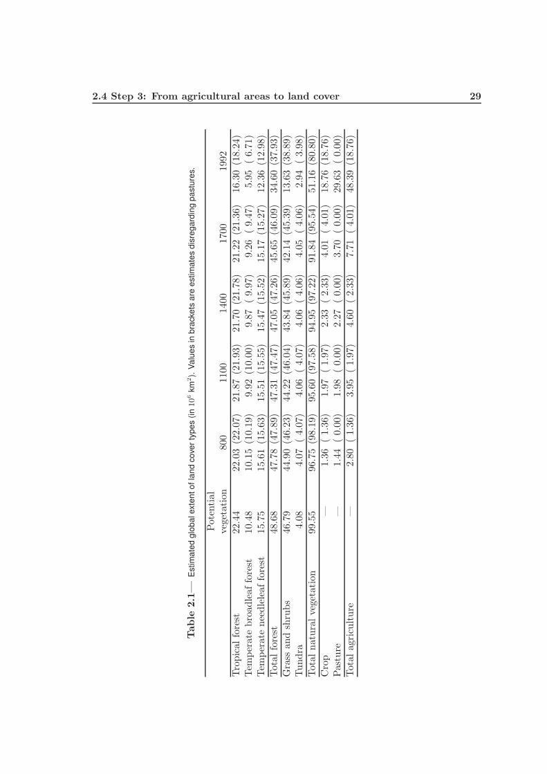
2.4 Step 3: From agricultural areas to land cover 29
Table
2.1
—E
stim
ate
dg
lob
ale
xte
nto
fla
nd
cove
rty
pe
s(i
n106
km
2).
Va
lue
sin
bra
cke
tsa
ree
stim
ate
sd
isre
ga
rdin
gp
astu
res.
Pot
ential
vege
tation
800
1100
1400
1700
1992
Tro
pic
alfo
rest
22.4
422
.03
(22.
07)
21.8
7(2
1.93
)21
.70
(21.
78)
21.2
2(2
1.36
)16
.30
(18.
24)
Tem
per
ate
bro
adle
affo
rest
10.4
810
.15
(10.
19)
9.92
(10.
00)
9.87
(9.
97)
9.26
(9.
47)
5.95
(6.
71)
Tem
per
ate
nee
dle
leaf
fore
st15
.75
15.6
1(1
5.63
)15
.51
(15.
55)
15.4
7(1
5.52
)15
.17
(15.
27)
12.3
6(1
2.98
)
Tot
alfo
rest
48.6
847
.78
(47.
89)
47.3
1(4
7.47
)47
.05
(47.
26)
45.6
5(4
6.09
)34
.60
(37.
93)
Gra
ssan
dsh
rubs
46.7
944
.90
(46.
23)
44.2
2(4
6.04
)43
.84
(45.
89)
42.1
4(4
5.39
)13
.63
(38.
89)
Tundra
4.08
4.07
(4.
07)
4.06
(4.
07)
4.06
(4.
06)
4.05
(4.
06)
2.94
(3.
98)
Tot
alnat
ura
lve
geta
tion
99.5
596
.75
(98.
19)
95.6
0(9
7.58
)94
.95
(97.
22)
91.8
4(9
5.54
)51
.16
(80.
80)
Cro
p—
1.36
(1.
36)
1.97
(1.
97)
2.33
(2.
33)
4.01
(4.
01)
18.7
6(1
8.76
)Pas
ture
—1.
44(
0.00
)1.
98(
0.00
)2.
27(
0.00
)3.
70(
0.00
)29
.63
(0.
00)
Tot
alag
ricu
lture
—2.
80(
1.36
)3.
95(
1.97
)4.
60(
2.33
)7.
71(
4.01
)48
.39
(18.
76)
30 2 MILLENNIUM LAND COVER RECONSTRUCTION
that does not return to potential vegetation, e.g. where forest re-establishment isinhibited through degraded soil conditions.
2.5 Assessing uncertainty and validity
The method developed in this study relies on only few, basic assumptions whenhistorical sources and modern estimates fail to provide the necessary information.The aim is to keep methods, results, and uncertainties at any time straightforwardand comprehensible. In the following, we discuss sources of possible errors and assessuncertainties associated with data and method.
2.5.1 Inclusiveness of the millennium reconstruction
This study focuses on anthropogenic land cover change that permanently changesthe type of vegetation, taking into account the permanent expansion and abandon-ment of cropland and pasture. Two important land use types, however, are notincluded: (1) Wood harvesting is not considered in this study. Our reconstructioncan be combined with wood harvest data once such statistics become available forpreindustrial times, but it should be kept in mind that the clearing of forest fortimber or fuelwood is not an entirely independent land use alongside agriculture. Apart of the area cleared for wood harvest is subsequently used for agriculture, andanother part is quickly regrown in a system of managed forest and does therefore notrepresent a permanent change of the type of vegetation. (2) The long-term fallowarea that results from shifting cultivation is not covered by this study. A sensitivityanalysis [Hurtt et al., 2006] showed that the omission of shifting cultivation may leadto a significant underestimation of secondary land area created by agriculture, butthe very high resolution data needed to resolve such small-scale processes is usuallynot available for large regions. However, shifting cultivation only increases the areaundergoing gross transition, while net transition, as represented by our data set, isunaffected. Similarly, the representation of wood harvest would only alter the area ofundisturbed vegetation, but not the area estimates of cropland and pasture derivedin this study. Therefore, our results for cropland and pasture remain valid withinthe accuracies discussed in the following, as long as no subnational and sub-gridinformation is derived.
2.5.2 Validation of the base data AD 1700 to 1992
Ramankutty and Foley [1998] compared their remote-sensing-based cropland map of1992 to three other estimates and conclude that their data set provides a “reasonablyaccurate and quantitative depiction of croplands across the globe”. The SAGEmaps have also been compared to the HYDE data for cropland in both presentand historical times (for details, see Klein Goldewijk and Ramankutty [2004] andRamankutty et al. [2006]). They are found to be generally consistent with HYDEin representing cropland over the last 300 years. A strong caveat of this comparison
2.5 Assessing uncertainty and validity 31
is the fact that the two data sets are not entirely independent and partially rely onthe same input data. The SAGE time series has further been proven to representcommon knowledge about the evolution of cropland in different parts of the world[Ramankutty and Foley, 1999].
Few independent data sets exist that could be used to validate the pattern ofpasture. It is often impossible to distinguish between pristine grasslands and suchused for grazing (pasture) in observation data, and classification strongly dependson subtleties in definition. When compared to the HYDE data (revised version3.0, K. Klein Goldewijk, personal communication), the present-day pasture extentof Foley et al. [2003] agrees well in Europe, America and Africa, though in thelatter the HYDE data concentrates pasture more strongly in the Maghreb coast andthe Sahel. Some differences exist in the Middle East. Especially the semi-desertand desert of the Arabian peninsula show much higher intensities of pasture in theHYDE data, while the SAGE map is more closely coupled to the maximum possiblevegetation cover. We believe that this is the more appropriate pattern for historicaltimes, where population pressure was low and less suitable areas did not have tobe included into agricultural activity. The interior of the Australia continent is lessintensely used for pasture in the SAGE data, but this discrepancy is unimportant forhistorical times as Aboriginal agricultural activity was very low. The most extensivepasture lands in Mongolia and Tibet are identified in both SAGE and HYDE 3.0,but with a higher intensity in the SAGE data. In our reconstruction, this highintensity reflects back to historical times.
We conclude that the overall pattern of cropland and pasture of Ramankutty andFoley [1998, 1999] and Foley et al. [2003] are in good agreement with other studies.This is an important point, as historical patterns are derived from present day datain both the SAGE approach and our method and errors would propagate to earliertimes. Concerning total agricultural areas, some uncertainty exists not only forpast, but also present times. In absolute numbers, the 1992 Ramankutty and Foleymap used in this study (including the modifications described in Sec. 2.2) shows acropland area of 18.8 ·106 km2, while estimates by Richards [1990] for the year 1980are 15.0 ·106 km2, by Houghton [1999] for the year 1990 are 13.6 ·106 km2, and byKlein Goldewijk [2001] for the year 1990 are 14.7 ·106 km2 (note that all estimatespartially rely on the same input data). The pasture map used in this study showsan area of 29.6 ·106 km2 as opposed to the estimate of Klein Goldewijk [2001] forthe year 1990 of 34.5 ·106 km2. Obviously, notable uncertainties exist despite thegrowing availability of ground- and satellite-based observations and internationalstatistical databases. We cannot assume that data uncertainties are any smallerbetween AD 1700 and 1992 than at present. As this time series is also the base datafor our reconstruction, this uncertainty is passed on to all earlier time steps.
2.5.3 Uncertainty of the population data
Despite the long tradition of demographic research, no outright consensus existsconcerning quantitative estimates of historical population, especially for times earlier
32 2 MILLENNIUM LAND COVER RECONSTRUCTION
than the 18th century. Global numbers differ by up to a factor of two for thefirst millennium AD; regional estimates can be even more disputed. The data setpredominantly used in this study [McEvedy and Jones, 1978] is largely acknowledgedin recent literature and stands out through its consistency and high spatial andtemporal resolution. The uncertainties introduced by the choice of this specificpopulation database are estimated in the following.
The population database of this study is compared to six other historical es-timates (Clark [1967], Biraben [1979], Maddison [2001], and high, mean, and lowestimates by Durand [1977]). For the Americas, we further include the originaldata from McEvedy and Jones [1978] without our modifications. Data for the yearsAD 1000, 1500 and 1700 are used in aggregated form for four regions following Mad-dison [2001] (Tab. A.1). There is good agreement between the studies with respectto Europe and Asia, where estimates differ by less than a factor of 2 even for earlyyears. Not surprisingly, however, large differences exist for Africa and the Americas,where much of the continents was still unexplored by the end of the 17th century.Still in debate, for example, is the number of native Americans prior to Europeanarrival, where estimates range between 14 and 63 million, as well as the rate ofpopulation growth before.
The population dynamics of the temporally highly-resolved data used in thisstudy are superimposed on the alternative estimates. Then, for each year and eachregion the two data sets are chosen that give the highest and lowest changes in pop-ulation relative to their AD 1700 value. This method thus results in an uncertaintyrange around the population estimates used for the millennium reconstruction. Itis important to note that the extreme ranges do not represent consistent time seriesof likely alternative scenarios. Rather, they indicate the entire range of possibleestimates of agricultural areas for a given year, where the outer bounds can only bereached for a certain time period throughout the millennium, if at all. The maxi-mum uncertainty range we assign to the persistent estimate due to uncertainties inpopulation estimates, based on the described approach, for the year AD 800 is 1.1to 1.6 ·106 km2 around the persistent estimate of 1.4 ·106 km2 for crop, and 1.1 to1.7 ·106 km2 around the estimate of 1.4 ·106 km2 for pasture. In relative terms, thelargest underestimation that could occur in AD 800 due to errors in the populationdata used in this study is in the Americas. Here, the high estimate of Durand [1977]does acknowledge that there has been significant decrease in population with Eu-ropean conquest, but believes in steadily high population before that. The largestoverestimation of our study could occur in Africa. Here, Biraben [1979] suggestsmuch stronger population dynamics prior to AD 1700 than all other data sets.
2.5.4 Effects of agrotechnical improvements
A major assumption of our approach in reconstructing historical agricultural areasis that the ratio of agricultural areas per capita did not change prior to AD 1700.Agricultural areas per person is the inverse of nutritional density and corresponds toland (not labor) productivity — per-area yields — in the absence of major dietary
2.5 Assessing uncertainty and validity 33
changes and trade. Dietary changes and trade are considered to be minor drivers ofchanges in agricultural areas in the time period under investigation. Trade, specifi-cally, was largely limited to high-value products such as silk, wool, and spices, unlesswater transport became possible, as costs of transport prior to the 19th century weretoo high to move general foodstuff [Grigg, 1974]. Theory predicts that land produc-tivity increases within a civilization as agrotechnical innovations are continuouslytriggered through population pressure and shortages [Boserup, 1965, Sieferle, 1997],but published data is not sufficiently available for use in a consistent global analysisand is frequently in contradiction to theory [Slicher van Bath, 1963].
Nevertheless, an estimate of the uncertainties of the persistent estimate of themillennium reconstruction is desireable. For this, we recalculate crop area withina maximum range of possible changes in per-capita values of cropland. In thesevalues, we try to not only include agrotechnical progress, but also regression dueto land degradation and socioeconomic disturbances, changes in crop types, andchanges in the fraction of population incorporated in an agricultural system forthose regions where we know that these factors play a non-negligible role. Based onthese factors, we try to give an upper and lower boundary of possible changes in per-capita cropland. Where available, we base our estimates on quantitative data, suchas yield ratios from Slicher van Bath [1963] for European countries and nutritionaldensities cited in Grigg [1974] for East Asian countries. Where quantitative data ismissing, we classify regions as one of three cases based on the information of Grigg[1974] and Vasey [1992]: regions with general decrease in per-capita cropland values(range of 0.7 to 1.7 in AD 800 relative to AD 1700 around the persistent estimate),with no change (0.5–1.5), and with general increase (0.3–1.3) (see Tab. A.2; fordetails see Pongratz et al. [2008a]). With these numbers, the time period underconsideration is characterized as a period where the overall pace of technologicalchange in farming has been “remarkably slow” [Grigg, 1974, p. 50] and most ofthe preindustrial increases in crop and animal production occurred as a result ofincreases in agricultural areas [Ruttan, 2002].
Changes in the per-capita use of pastures have not been assessed for historicaltimes in literature. Here, we generally use the same ranges for pastures as forcropland. Most factors affecting changes in cropland per person will also affect theuse of pasture. Changes in productivity will be less pronounced than for crop, butthe general trend may be similar, since many agrotechnical improvements such asmanuring can also be applied to forage crops and the number of draught animalsper capita is linked to cropland productivity.
The maximum uncertainty range we assign to the persistent estimate due tochanges in per-capita agricultural areas, for the year AD 800, is 0.8 to 2.2 ·106 km2
around the persistent estimate of 1.4 ·106 km2 for crop, and 0.8 to 2.1 ·106 km2
around the estimate of 1.4 ·106 km2 for pasture. Changes in the agricultural sys-tems of the world thus introduce a significantly higher uncertainty in our approachthan the decision for a specific population data set. Except for the Americas, thisstatement also holds true at regional level. This difference can largely be explainedby the fact that population data itself is less uncertain than information on per-
34 2 MILLENNIUM LAND COVER RECONSTRUCTION
capita agricultural area. The reasons for this include a greater administrative in-terest in documenting population throughout history in combination with a muchbetter agreement on the definition of “population” than of “agricultural area” or“yields”. Furthermore, the spatial coverage is higher for population estimates, whichare usually documented at a regional scale. On the other hand, information on theper-capita demand of agricultural area has to be extrapolated from local measure-ments and qualitative descriptions, which was done in a conservative way in thisstudy. For the following analysis of historical land cover change, we combine bothuncertainty factors, per-capita agricultural areas and population, in a way that re-sults in the maximum possible range at every timestep in every part of the world.Joining highest agrotechnical progress with lowest population growth and vice versagive possible, but unlikely estimates of agricultural areas. This range of uncertaintyassigned to the persistent estimate therefore does not indicate a range of equal pref-erence, which would be much smaller. Instead, it is intended to define limits ofpossible errors in the estimates caused by our approach. We did not assign an un-certainty range to the base data AD 1700 to 1992, but it should be kept in mindthat errors in the maps of AD 1700 propagate back in time (Sec. 2.5.2).
2.6 Changes in land cover AD 800–1992
We present our reconstructions in two ways: The full spatial information is depictedin the maps for historical crop and pasture in Figs. 2.2 and 2.3, shown for four timeslices. More information about the temporal evolution of cropland and pasture arepresented in Figs. 2.4 and 2.5. Here, the total areas of the agricultural types and thenatural vegetation types are plotted for 10 world regions. The persistent estimatesare surrounded by the range which was determined from the uncertainties in ourmethod associated with population data as well as changes in per-capita agriculturalareas (see Sec. 2.5). Additionally shown with the natural vegetation types is thepersistent estimate for land cover change due to the expansion of cropland only,disregarding pasture. It is thus possible to separate the impact of changes in croplandon natural vegetation from the impact of changes in pasture.
We can compare the millennium reconstruction against the common knowledgeabout the history of agriculture in order to test its plausibility and interpret ourresults. The map for AD 800 (Fig. 2.2) clearly highlights the regions with thelongest history of agriculture: High intensities of crop cultivation are found in theMediterranean, the Fertile Crescent, and India. Large areas of cropland are alsodeduced for China. In all these regions, the domestication of crops or the spread ofcrops into the region had taken place thousands of years ago [Vasey, 1992]. On theother hand, many parts of the world show little human impact in the map of AD 800.Agriculture had developed early also in the Americas, but intensity remained lowoutside the centers of high cultures until Europeans arrived [Grigg, 1974]. Mostof central Asia was not settled until the 19th century, and the agricultural tribesin Australasia were few and low in numbers [McEvedy and Jones, 1978]. Much
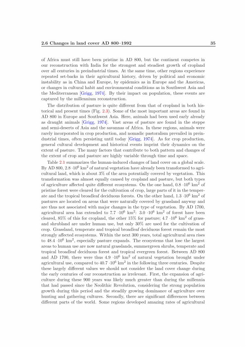
2.6 Changes in land cover AD 800–1992 35
of Africa must still have been pristine in AD 800, but the continent competes inour reconstruction with India for the strongest and steadiest growth of croplandover all centuries in preindustrial times. At the same time, other regions experiencerepeated set-backs in their agricultural history, driven by political and economicinstability as in China and Europe, by epidemics as in Europe and the Americas,or changes in cultural habit and environmental conditions as in Southwest Asia andthe Mediterranean [Grigg, 1974]. By their impact on population, these events arecaptured by the millennium reconstruction.
The distribution of pasture is quite different from that of cropland in both his-torical and present times (Fig. 2.3). Some of the most important areas are found inAD 800 in Europe and Southwest Asia. Here, animals had been used early alreadyas draught animals [Grigg, 1974]. Vast areas of pasture are found in the steppeand semi-deserts of Asia and the savannas of Africa. In these regions, animals wererarely incorporated in crop production, and nomadic pastoralism prevailed in prein-dustrial times, often persisting until today [Grigg, 1974]. As for crop production,general cultural development and historical events imprint their dynamics on theextent of pasture. The many factors that contribute to both pattern and changes ofthe extent of crop and pasture are highly variable through time and space.
Table 2.1 summarizes the human-induced changes of land cover on a global scale.By AD 800, 2.8 ·106 km2 of natural vegetation have already been transformed to agri-cultural land, which is about 3% of the area potentially covered by vegetation. Thistransformation was almost equally caused by cropland and pasture, but both typesof agriculture affected quite different ecosystems. On the one hand, 0.8 ·106 km2 ofpristine forest were cleared for the cultivation of crop, large parts of it in the temper-ate and the tropical broadleaf deciduous forests. On the other hand, 1.3 ·106 km2 ofpastures are located on areas that were naturally covered by grassland anyway andare thus not associated with major changes in the type of vegetation. By AD 1700,agricultural area has extended to 7.7 ·106 km2: 3.0 ·106 km2 of forest have beencleared, 85% of this for cropland, the other 15% for pasture; 4.7 ·106 km2 of grass-and shrubland are under human use, but only 30% are used for the cultivation ofcrop. Grassland, temperate and tropical broadleaf deciduous forest remain the moststrongly affected ecosystems. Within the next 300 years, total agricultural area risesto 48.4 ·106 km2, especially pasture expands. The ecosystems that lose the largestareas to human use are now natural grasslands, summergreen shrubs, temperate andtropical broadleaf deciduous forest and tropical evergreen forest. Between AD 800and AD 1700, there were thus 4.9 ·106 km2 of natural vegetation brought underagricultural use, compared to 40.7 ·106 km2 in the following three centuries. Despitethese largely different values we should not consider the land cover change duringthe early centuries of our reconstruction as irrelevant. First, the expansion of agri-culture during these 900 years was likely much greater than during the millenniathat had passed since the Neolithic Revolution, considering the strong populationgrowth during this period and the steadily growing dominance of agriculture overhunting and gathering cultures. Secondly, there are significant differences betweendifferent parts of the world. Some regions developed amazing rates of agricultural
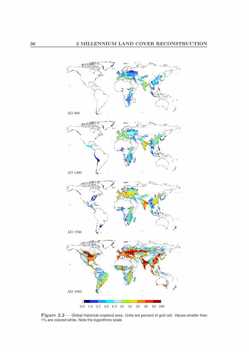
36 2 MILLENNIUM LAND COVER RECONSTRUCTION
AD 800
AD 1400
AD 1700
AD 1992
0.0 1.6 2.5 4.0 6.3 10 16 25 40 63 100
Figure 2.2— Global historical cropland area. Units are percent of grid cell. Values smaller than
1% are colored white. Note the logarithmic scale.

2.6 Changes in land cover AD 800–1992 37
AD 800
AD 1400
AD 1700
AD 1992
0.0 1.6 2.5 4.0 6.3 10 16 25 40 63 100
Figure 2.3— Global historical pasture area. Units are percent of grid cell. Values smaller than
1% are colored white. Note the logarithmic scale.
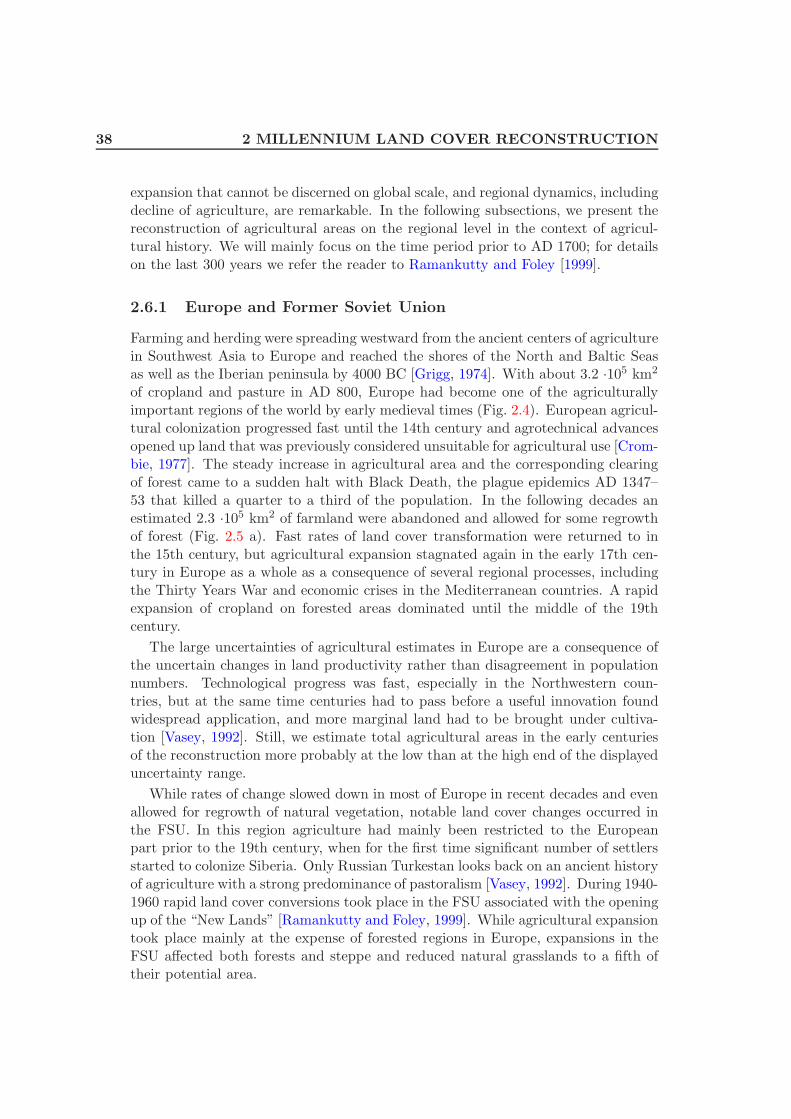
38 2 MILLENNIUM LAND COVER RECONSTRUCTION
expansion that cannot be discerned on global scale, and regional dynamics, includingdecline of agriculture, are remarkable. In the following subsections, we present thereconstruction of agricultural areas on the regional level in the context of agricul-tural history. We will mainly focus on the time period prior to AD 1700; for detailson the last 300 years we refer the reader to Ramankutty and Foley [1999].
2.6.1 Europe and Former Soviet Union
Farming and herding were spreading westward from the ancient centers of agriculturein Southwest Asia to Europe and reached the shores of the North and Baltic Seasas well as the Iberian peninsula by 4000 BC [Grigg, 1974]. With about 3.2 ·105 km2
of cropland and pasture in AD 800, Europe had become one of the agriculturallyimportant regions of the world by early medieval times (Fig. 2.4). European agricul-tural colonization progressed fast until the 14th century and agrotechnical advancesopened up land that was previously considered unsuitable for agricultural use [Crom-bie, 1977]. The steady increase in agricultural area and the corresponding clearingof forest came to a sudden halt with Black Death, the plague epidemics AD 1347–53 that killed a quarter to a third of the population. In the following decades anestimated 2.3 ·105 km2 of farmland were abandoned and allowed for some regrowthof forest (Fig. 2.5 a). Fast rates of land cover transformation were returned to inthe 15th century, but agricultural expansion stagnated again in the early 17th cen-tury in Europe as a whole as a consequence of several regional processes, includingthe Thirty Years War and economic crises in the Mediterranean countries. A rapidexpansion of cropland on forested areas dominated until the middle of the 19thcentury.
The large uncertainties of agricultural estimates in Europe are a consequence ofthe uncertain changes in land productivity rather than disagreement in populationnumbers. Technological progress was fast, especially in the Northwestern coun-tries, but at the same time centuries had to pass before a useful innovation foundwidespread application, and more marginal land had to be brought under cultiva-tion [Vasey, 1992]. Still, we estimate total agricultural areas in the early centuriesof the reconstruction more probably at the low than at the high end of the displayeduncertainty range.
While rates of change slowed down in most of Europe in recent decades and evenallowed for regrowth of natural vegetation, notable land cover changes occurred inthe FSU. In this region agriculture had mainly been restricted to the Europeanpart prior to the 19th century, when for the first time significant number of settlersstarted to colonize Siberia. Only Russian Turkestan looks back on an ancient historyof agriculture with a strong predominance of pastoralism [Vasey, 1992]. During 1940-1960 rapid land cover conversions took place in the FSU associated with the openingup of the “New Lands” [Ramankutty and Foley, 1999]. While agricultural expansiontook place mainly at the expense of forested regions in Europe, expansions in theFSU affected both forests and steppe and reduced natural grasslands to a fifth oftheir potential area.
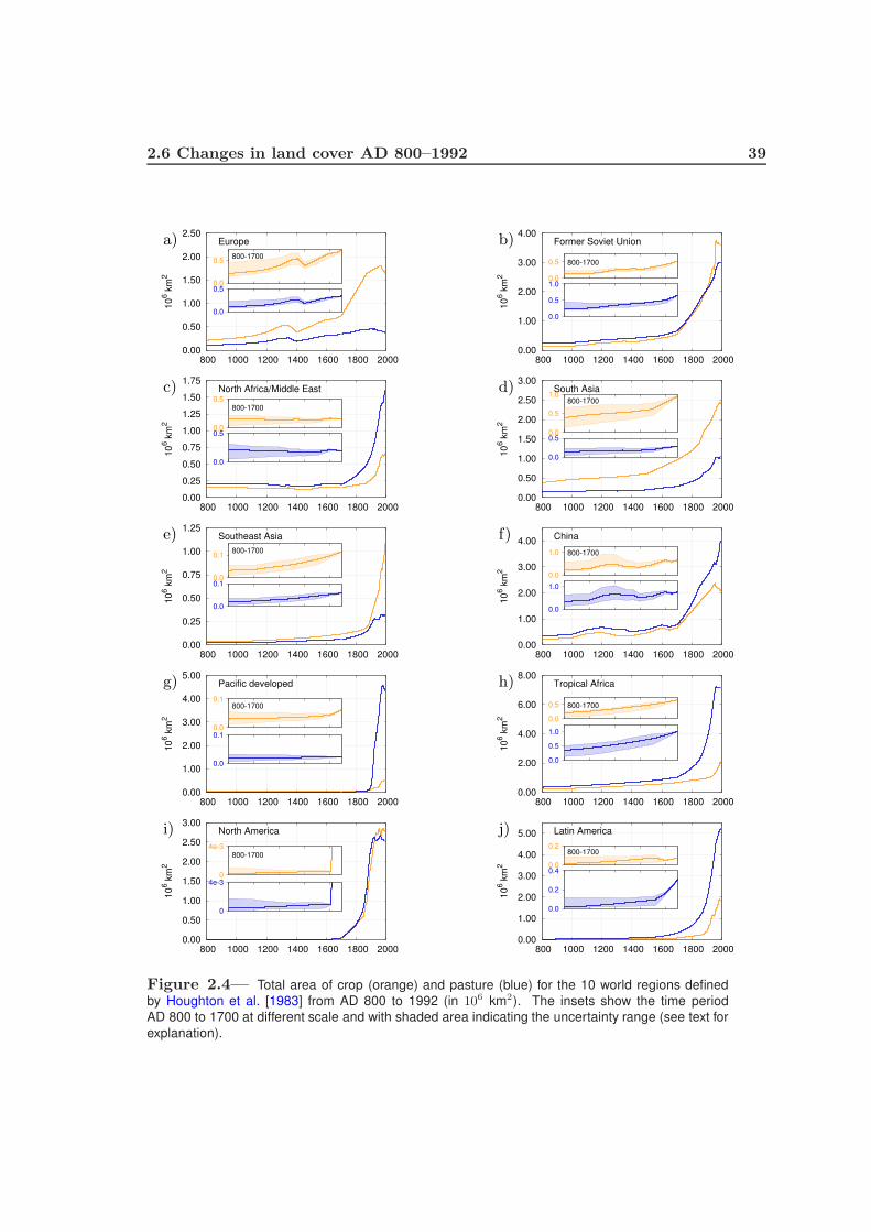
2.6 Changes in land cover AD 800–1992 39
0.00
0.50
1.00
1.50
2.00
2.50
800 1000 1200 1400 1600 1800 2000
10
6 k
m2
Europe
0.0
0.5800-1700
0.0
0.5
a)
0.00
1.00
2.00
3.00
4.00
800 1000 1200 1400 1600 1800 2000
10
6 k
m2
Former Soviet Union
0.0
0.5 800-1700
0.0
0.5
1.0
b)
0.00
0.25
0.50
0.75
1.00
1.25
1.50
1.75
800 1000 1200 1400 1600 1800 2000
10
6 k
m2
North Africa/Middle East
0.0
0.5800-1700
0.0
0.5
c)
0.00
0.50
1.00
1.50
2.00
2.50
3.00
800 1000 1200 1400 1600 1800 20001
06 k
m2
South Asia
0.0
0.5
1.0800-1700
0.0
0.5
d)
0.00
0.25
0.50
0.75
1.00
1.25
800 1000 1200 1400 1600 1800 2000
10
6 k
m2
Southeast Asia
0.0
0.1800-1700
0.0
0.1
e)
0.00
1.00
2.00
3.00
4.00
800 1000 1200 1400 1600 1800 2000
10
6 k
m2
China
0.0
1.0 800-1700
0.0
1.0
f)
0.00
1.00
2.00
3.00
4.00
5.00
800 1000 1200 1400 1600 1800 2000
10
6 k
m2
Pacific developed
0.0
0.1800-1700
0.0
0.1
g)
0.00
2.00
4.00
6.00
8.00
800 1000 1200 1400 1600 1800 2000
10
6 k
m2
Tropical Africa
0.0
0.5 800-1700
0.0
0.5
1.0
h)
0.00
0.50
1.00
1.50
2.00
2.50
3.00
800 1000 1200 1400 1600 1800 2000
10
6 k
m2
North America
0
4e-3800-1700
0
4e-3
i)
0.00
1.00
2.00
3.00
4.00
5.00
800 1000 1200 1400 1600 1800 2000
10
6 k
m2
Latin America
0.0
0.2800-1700
0.0
0.2
0.4
j)
Figure 2.4— Total area of crop (orange) and pasture (blue) for the 10 world regions defined
by Houghton et al. [1983] from AD 800 to 1992 (in 106 km2). The insets show the time period
AD 800 to 1700 at different scale and with shaded area indicating the uncertainty range (see text for
explanation).
40 2 MILLENNIUM LAND COVER RECONSTRUCTION
2.6.2 North Africa/Middle East
In Southwest Asia lies one of the birthplaces of agriculture. Wild cereals were har-vested already in the 10th millennium BC and seed agriculture developed, associatedearly with the use of ploughs and draught animals [Grigg, 1974]. Intensive agricul-ture in AD 800 is restricted, however, to the Mediterranean coast and Anatolia,where climate is more favorable, and to the irrigated fields of Egypt and the Fer-tile Crescent (Figs. 2.2 and 2.3). The latter is the most intensely cultivated regionworld-wide at the beginning of our reconstruction, with crop fractions of up to 50%.This prominent role, however, is lost during the next few centuries, and a multi-tude of reasons led to stagnating agriculture also in the other regions of the MiddleEast and North Africa (Fig. 2.4 c). In Persia and Anatolia, Turkish invasions hadnegative effects on peasant activity, while North Africa was affected by the Bedouininvasion (11th century), the plague (14th century), and the Mediterranean economicrecession (17th century) [McEvedy and Jones, 1978]. In Egypt, all land was alreadyexploited as far as technology allowed. Crop and pasture thus remained at a rela-tively low extent for many centuries until population gradually grew from the 18thcentury onwards. With pastoralism being the dominant form of agriculture, muchnatural grassland was now used for grazing (Fig. 2.5 c). Crop production becamemore important in the 20th century, associated with a steep increase of population,and with it woody vegetation was reduced.
The long history of cultivation in this region most probably degraded land pro-ductivity in many regions, with salinization becoming a common problem in irrigatedareas. Permanent agriculture was frequently given up in favor of nomadism in timesof economic recession and warfare [Grigg, 1974]. Our persistent estimate thus lies atthe higher end of crop estimates, and uncertainties are large for natural and man-aged grassland areas. Errors in the population estimates play a minor role only —though absolute numbers are still subject to dispute, growth rates are rather similarin all literature estimates.
2.6.3 South Asia and Southeast Asia
The Indian subcontinent experienced peasant settlement in the 4th millennium BCin the Indus valley and around the 1st millennium BC in the Ganges valley [Grigg,1974]. By AD 800, South Asia was the major player in global crop production withabout 4.0 ·105 km2 of cultivated land (Fig. 2.4 d). Crop areas grew steadily, thoughat moderate pace first. Population most certainly has been set back several timesthroughout the centuries, but historical evidence is sparse [McEvedy and Jones,1978]. A significant part of the indicated uncertainties must thus be attributedto demographic data. From the 16th to the 19th century agricultural expansionaccelerated, significant amounts of forest were cleared for cropland, and grass andshrubland were used for grazing (Fig. 2.5 d). Under European control and afterindependence, the pattern became more complex with agricultural expansion set offby abandonments in various parts of India [Ramankutty and Foley, 1999].

2.6 Changes in land cover AD 800–1992 41
0.0
0.5
1.0
1.5
2.0
2.5
3.0
3.5
800 1000 1200 1400 1600 1800 2000
10
6 k
m2 Europe
a)
0.0
1.0
2.0
3.0
4.0
5.0
6.0
7.0
8.0
9.0
10.0
800 1000 1200 1400 1600 1800 2000
10
6 k
m2
Former Soviet Unionb)
0.0
0.5
1.0
1.5
2.0
2.5
3.0
800 1000 1200 1400 1600 1800 2000
10
6 k
m2 North Africa/Middle East
c)
0.0
0.5
1.0
1.5
2.0
2.5
3.0
800 1000 1200 1400 1600 1800 20001
06 k
m2
South Asia
d)
0.0
0.5
1.0
1.5
2.0
2.5
3.0
3.5
800 1000 1200 1400 1600 1800 2000
10
6 k
m2 Southeast Asia
e)
0.0
1.0
2.0
3.0
4.0
5.0
6.0
800 1000 1200 1400 1600 1800 2000
10
6 k
m2 China
f)
0.0
1.0
2.0
3.0
4.0
5.0
6.0
7.0
800 1000 1200 1400 1600 1800 2000
10
6 k
m2 Pacific developed
g)
0.0
2.0
4.0
6.0
8.0
10.0
12.0
14.0
800 1000 1200 1400 1600 1800 2000
10
6 k
m2 Tropical Africa
h)
0.0
1.0
2.0
3.0
4.0
5.0
6.0
7.0
8.0
9.0
800 1000 1200 1400 1600 1800 2000
10
6 k
m2
North America
i)
0.0
2.0
4.0
6.0
8.0
10.0
12.0
800 1000 1200 1400 1600 1800 2000
10
6 k
m2
Latin America
j)
Figure 2.5— Total area of natural vegetation: forest (green) and natural grassland, shrubland,
and tundra (blue), for the 10 world regions defined by Houghton et al. [1983] from AD 800 to 1992 (in
106 km2). Shaded area indicates the uncertainty range (see text for explanation). Dashed lines are
land cover change due to cropland only.

42 2 MILLENNIUM LAND COVER RECONSTRUCTION
Compared to the Indian subcontinent, agricultural activity was rather low inSoutheast Asia in AD 800 and remained so for the next thousand years. On theMalay Archipelago peasant population has always been concentrated on the southernislands [Grigg, 1974], a pattern reflected in Figs. 2.2 and 2.3. Much of the increasein cropland area that happened in Southeast Asia (Fig. 2.4 e) must be attributedto the spread of wet rice, which had been introduced from China or India about2000 years ago [Grigg, 1974]. Rice also has a key role in the high expansion rates ofcrop in the mainland countries in the 19th and 20th century. In recent decades, theSoutheast-Asian region has one of the highest deforestation rates globally. Pastureareas are small compared to cropland in Southeast Asia with a total of 3.1·105 km2
in 1992, but some of the highest stocking rates of the world are found in thesecountries [Asner et al., 2004].
2.6.4 China
An independent development of seed agriculture took place in Northern China in the5th and 6th millennia BC including the domestication of pigs, while tropical vegecul-ture was practiced further south [Grigg, 1974]. Based on these traditions, it is notsurprising that Chinese crop area was large by AD 800, estimated at 2.1 ·105 km2.Large-scale migration from the Yellow River south in the preceding centuries hadprobably led to a crop pattern similar to today, covering much of the Eastern part ofthe country. Not reflected in our pattern, however, is the following further concentra-tion of agriculture in the southeastern areas. With it, agricultural methods changednotably, with increasing focus on rice and the introduction of double-cropping. Thepossible range of crop area prior to the 14th century is thus large, and the persistentestimate is at its lower end (Fig. 2.4 f). Population data contributes only marginallyto the uncertainties thanks to meticulous dynastic censi. Two dramatic events in-terrupted the otherwise strong growth of population and agriculture: the countrylost about a third of its population in the course of the Mongol invasions startingin AD 1211, and again about a sixth of its population in the upheavals after thefall of the Ming Dynasty in 1644 [McEvedy and Jones, 1978]. Thereafter, growthwas resumed at unprecedented pace, and half of China’s natural forest cover wastransformed to cropland.
The 3.4 ·105 km2 of pasture in AD 800 is almost exclusively located in Mongo-lia and Tibet, where herding was the traditional form of agriculture well into the20th century. The large uncertainties of the estimates should be seen as tribute tonomenclature — nomadism makes it difficult even today to define permanent pas-tures. The expansion we see is largely at the expense of natural grassland or tundravegetation (Fig. 2.5 f).
2.6.5 Pacific Developed
A clear break occurs in the late 19th century in the developed countries of the Pacific,with very little agricultural area and dynamics over the preceding millennium and

2.6 Changes in land cover AD 800–1992 43
a steep increase of agriculture — mainly pasture — afterwards (Fig. 2.4 g). InJapan, the agricultural area needed per capita in AD 1700 is extraordinarily small,as fish has been a major part of the traditional diet and the main crop, rice, wascultivated with high nutritional density [Grigg, 1974]. We see notable increases inagriculture only after 1870. After 1945, Australia became the driving force of landcover change in the Pacific developed region. Crop expanded in the 19th centuryin Southeast Australia, later in Western Australia, affecting grass as well as woodyecosystems. An additional 4.1 ·106 km2 of pasture exist in 1992 in Australia, makingit the country with the most land area in pasture systems. For a large part naturalgrasslands were used as pastures, but also shrubland with woody vegetation, whichwas not always permanently cleared for herding. The reduction in shrubland seen inFig. 2.5 g for the last century may thus be overestimated when defining pastures asopen grassland. New Zealand shows a similar trend in crop and pasture as Australia,though at much smaller absolute numbers.
2.6.6 Tropical Africa
By 1700 the region south of the Sahel was still largely unexplored outside the coastalregions and population numbers and agricultural habits are still a matter of dispute.Vegeculture must have existed from the 5th millennium BC onwards in West Africaand cereal cultivation developed in the Horn region. The Northern savannas wereagriculturally used by the 3rd or 2nd millennium BC [Grigg, 1974]. The Bantuexpansion is one of the key factors in spreading cereal cultivation, pastoralism andiron technology throughout much of sub-Saharan Africa [Grigg, 1974, Hanotte et al.,2002], and with it the pattern of agriculture may have been subject to some changeespecially in the early centuries of our reconstruction. The uncertainty range sug-gests lower values for cropland and pasture extent to account for the possibility thatBantu culture gradually replaced cultures based on hunting and gathering. Muchof the uncertainty in this part of the world, however, is due to contradictory popu-lation estimates ranging, e.g., between 25 and 50 million for AD 1000 (see auxiliarymaterial Tab. A.1).
In general, we observe a steady increase of agriculture in all countries of tropi-cal Africa, which comprises the most different cultures, some of which are almostexclusively depending on herding while others mix husbandry with significant culti-vation [Vasey, 1992]. Animal husbandry is and has always been a significant sectorof agriculture in this part of the world, and pasture features as the dominant typeof agriculture in West Africa, the Horn and Southwest Africa in the early centuriesof our reconstruction (Fig. 2.3). Grazing focuses on the vast savanna regions andit seems reasonable to assume that their woody fractions are notably affected onlyduring the last two centuries, with the onset of exponential population growth andincreasing pressure on ecosystems. Figure 4 h shows that the expansion of pasturecame to a halt in the 1960s, while croplands further increased. The pattern of crop-land changed to form new centers in South Africa, the Lake Victoria region, andNigeria, though much of today’s crop cover in tropical Africa still remains under low
44 2 MILLENNIUM LAND COVER RECONSTRUCTION
intensity subsistence farming [Ramankutty and Foley, 1999].
2.6.7 The Americas
While there was a lively dispersal of domesticated plants and animals across the OldWorld, the Americas developed their very own forms of agriculture. First evidenceof plant domestication stems from Meso-America and coastal Peru in the 6th and5th millennium BC [Grigg, 1974]. In Central and South America, notable crop-land intensities developed only within the high cultures, while outside these regionslow-intensity swidden cultivation was practiced (Fig. 2.2). Crop areas grew to some0.8 ·105 km2 in our estimates by AD 1500. Pasture at the same time is estimatedto be 0.9 ·105 km2 and located mainly on the grasslands in the Andes, where somepeoples are known to have kept cameloids [Vasey, 1992]. The uncertainty rangearound these estimates, however, is large despite the small total area, owing to thehistorians’ dispute about pre-Columbian population (Sec. 2.5.3). Significant agricul-tural areas must have been abandoned with the reduction of the native populationby European weapons and diseases, seen as a decrease in crop estimates in Fig. 2.4 j.Under European rule started a large-scale transformation of natural vegetation forcrop cultivation as well as for ranching, and agricultural areas were shifted from theWest towards the East coast (Figs. 2.2 and 2.3). Much of the natural grasslands ofthe steppe and savanna is used today for grazing (Vasey [1992], Fig. 2.5 j).
In North America, some clearing of natural vegetation took place in a kind ofswidden system, but wild food remained important [Vasey, 1992]. The spatial pat-tern and the distinct cultures of the different indigenous peoples in North Americaare not resolved by our global reconstruction, which should thus not be applied insmall-scale studies in this part of the world prior to colonization. The new diseasesfollowing first European contact brought population growth to a halt, but NorthAmerica was affected less severely than Central and South America. With the col-onization in the 17th century the European form of agriculture was introduced tothe East Coast and subsequently spread west. Growth rates of agricultural areaare high in the following centuries as a result of both increasing population and thegrowing dominance of agriculture over hunting and gathering. While the crop mapsof Ramankutty and Foley [1999] are based on state-level data from 1850 onwardsand are thus able to display this relocation, our algorithm for historical pasture isbased on national totals. Some of the grassland in the Great Plains and further west,which Fig. 2.3 classifies as pasture in AD 1800, was thus probably still pristine, andpastures were located further east instead. Robust features, after centuries of verylow agricultural activity, are the steep increase of cropland and pasture extent oncontinental scale during the 18th and 19th century with stagnating numbers in the20th century.
2.7 Conclusion 45
2.7 Conclusion
This study has presented a consistent approach to reconstruct global historical areasof cropland and pasture for time periods where agricultural data is scarce. Country-based population estimates have been used as proxy for agricultural activity. Amethod, based on few, basic assumptions, has been developed that allows to con-sistently translate these population data into estimates of extent of cropland andpasture. Its transparency allows to easily identify possible errors in each region, andwe have tried to specify the uncertainties associated with our approach. Data setsfor the highest and lowest possible agricultural estimates have been provided thatcan be used for sensitivity studies in further applications. The reconstruction showsthat global land cover change was small between AD 800 and AD 1700 comparedto industrial times. Compared to previous millennia, however, land cover changeduring the preindustrial time period of the last millennium must have been large,and notable fluctuations and distinct histories of agriculture are revealed on regionalscales.
There are no global data available that could be used to validate our reconstruc-tion. Local studies can be found for specific time periods, but the subnational scaleis not the proper basis for comparison. Except for a few regions, no subnational datawere included in our approach, so that meaningful tests can be performed only at thecountry level or higher. Once independent estimates of historical agricultural extentfrom proxies such as pollen profiles, archeological evidence, and historical recordsbecome available for larger regions, we hope to compare our reconstruction againstthese estimates. The results of the millennium reconstruction are, however, in gen-eral agreement with common knowledge about the history of agriculture, and we areconfident that our approach captures the global pattern of changes in agriculturalareas and gives a sound approximation of the regional dynamics.
In addition to reconstructing historical agricultural areas, estimates of human-induced changes in natural vegetation cover have also been derived. They providea better picture of what types of vegetation were transformed to cropland and topasture. Our estimates show that up to AD 1700 temperate and tropical broadleafdeciduous forests were most severely affected by crop cultivation, while large areasof natural grassland were used as pasture.
The history of agriculture and anthropogenic land cover change is interesting inits own right. Additionally, its knowledge is an essential prerequisite to assess earlyhuman impact on the environment. In combination with ecosystem and climatemodels, geographically explicit data sets like the reconstruction presented in thisstudy can be used to estimate the effects of preindustrial land cover change e.g.on hydrology, nutrient cycles, and regional to global climate. They can therebycontribute to a better understanding of the human role in past changes of the Earthsystem.
A digital version of the millennium reconstruction of global agricultural ar-eas and land cover is available from the World Data Center for Climate (DOI:
46 2 MILLENNIUM LAND COVER RECONSTRUCTION
10.1594/WDCC/RECON LAND COVER 800-1992). Please contact the authorsfor further information.
Acknowledgements
The authors would like to thank Pavel Tarasov and Andreas Dix for their valuablesuggestions on our reconstruction method. We are grateful to Navin Ramankuttyfor providing us with the SAGE 5 min and West Africa crop maps and his usefulcomments on them. We would like to thank Kees Klein Goldewijk for sharing hisexpert knowledge on historical agriculture and providing us with the HYDE 3.0version, and Alberte Bondeau for her valuable suggestions on pasture data.
47
Chapter 3
Radiative Forcing fromAnthropogenic Land CoverChange since AD 800
Abstract
We calculate the radiative forcing (RF) from surface albedo changes over the lastmillennium applying a recently published, population-based reconstruction of an-thropogenic land cover change (ALCC). This study thus allows for the first time toassess anthropogenic effects on climate during the preindustrial era at high spatialand temporal detail. We find that the RF is small throughout the preindustrialperiod on the global scale (negative with a magnitude less than 0.05 W/m2) and notstrong enough to explain the cooling reconstructed from climate proxies betweenAD 1000 and 1900. For the regional scale, however, our results suggest an early an-thropogenic impact on climate: Already in AD 800, the surface energy balance wasaltered by ALCC at a strength comparable to present-day greenhouse gas forcing —e.g. −2.0 W/m2 are derived for parts of India for that time. Several other regionsexhibit a distinct variability of RF as a result of major epidemics and warfare, withRF changes in the order of 0.1 W/m2 within just one century.
3.1 Introduction
Anthropogenic land cover change (ALCC) represents one of the most substantialhuman impacts on the Earth system. The large-scale transformation of naturalecosystems to managed areas alters climate through several pathways: First, bio-geochemical cycles are severely disturbed; e.g. ALCC caused about 35% of theanthropogenic CO2 emissions during the last 150 years [Houghton, 2003]. Second,climate is directly influenced by the modification of the physical properties of theland surface such as albedo, roughness, and evapotranspiration. Modeling studiessuggest that through these biogeophysical effects ALCC at mid- and high latitudes
48 3 RADIATIVE FORCING FROM LAND COVER CHANGE
induces a cooling [e.g. Bonan et al., 1992, Claussen et al., 2001, Bounoua et al.,2002]. This is explained by the increase of albedo associated with deforestation,which is caused by the snow masking effect of forest as well as by the higher snow-free albedo of non-forest vegetation. With the strong hydrological cycle in the tropicsthe reduction of roughness, leaf area, and rooting depth by deforestation reduces theevapotranspiration stronger than in the extra-tropics. The loss of evaporative cool-ing may thus compensate the albedo effect in the tropics so that ALCC can evenlead to a local warming [e.g. Claussen et al., 2001, Bounoua et al., 2002, DeFrieset al., 2002]. On the global scale, the opposing biogeophysical effects of ALCC widelycancel each other, but regional climate is significantly influenced by ALCC and mayeven affect remote areas via teleconnections [e.g. Chase et al., 2000].
While ALCC has been recognized as a key factor for present climate change, itsrole for historical climate is less clear. Concerning biogeophysical effects, most stud-ies suggest a global cooling as a result of the albedo changes from the dominatingmidlatitudinal deforestation. The European ”Medieval Warm Period” as well asthe long-term cooling during the middle of the last millennium may largely be ex-plained by the land cover changes over this period [Govindasamy et al., 2001, Goosseet al., 2006]. Also Brovkin et al. [1999] obtain biogeophysical cooling from historicalALCC, most strongly in the northern mid- and high latitudes. They show that theimpact of historical ALCC on climate is of comparable size as concurrent changesof other climate forcings, e.g. solar irradiance and atmospheric CO2, and is crucialfor reproducing historical climate. From these studies we conclude that historicalALCC may have important impacts on regional and possibly global climate throughits biogeophysical effects on the atmosphere. However, all previous studies coveringthe last millennium are based on ad hoc approximations of historical ALCC. In thisstudy, we use a recently published high-resolution reconstruction of ALCC for thelast millennium to address the climate impact from historical ALCC at high spatialdetail over the course of the history.
For this assessment we apply the radiative forcing (RF) measure, which is calcu-lated as the change in the net shortwave radiation flux at the tropopause after theforcing agent is introduced but prior to any climate feedbacks. In the case of landcover change, the RF is usually determined for the change in surface albedo. Studieshave shown that the RF concept is less well applicable to ALCC than to the classicclimate forcings such as well-mixed greenhouse gases: First, biogeophysical effectsof land cover change other than albedo changes may also impose climate forcings,e.g. changes in evapotranspiration and non-radiative processes [Pielke et al., 2002,Davin et al., 2007]. The albedo effect has, however, been shown to be dominanton global scale [Betts et al., 2007]. Second, the biogeochemical forcing counteractsbiogeophysics, with a similar strength on the global mean [Brovkin et al., 2004],but with much less regional heterogeneity. It is, however, usually treated separatelyfrom the biogeophysics due to its different nature of processes and impacts and isnot considered in this study. Third, the common application of RF to global meanclimate may underestimate the impact of ALCC, as ALCC is a spatially highlyheterogeneous perturbation where regional effects often differ in sign, so that they
3.2 Radiative forcing calculations 49
cancel out on global average despite possibly large regional climate impacts. ALCCthus requires a regionally explicit analysis. Nevertheless, the RF concept and itsapplication to albedo changes remain a standard tool to assess the importance ofALCC for climate [Forster et al., 2007], and has frequently been applied to quantifythe effects of ALCC on climate for the last 300 years [e.g. Myhre and Myhre, 2003,Betts et al., 2007]. By applying this measure to the entire last millennium, ourstudy allows to consistently compare preindustrial effects of ALCC to publicationscovering the industrial period.
3.2 Radiative forcing calculations
The RF calculations are performed with the land surface scheme JSBACH [Raddatzet al., 2007] coupled to the climate model ECHAM5 [Roeckner et al., 2003] at ahorizontal resolution of T63 (equivalent to about 1.8 degree) with 31 vertical levels.Atmospheric greenhouse gas concentrations, sea ice cover, and sea surface tempera-ture are prescribed to present-day conditions. Computation of the surface shortwaveradiation budget includes a spatially-explicit surface albedo calculation for the nearinfrared as well as the visible range. It depends on the albedo of the soil surface[Rechid et al., 2008], snow cover, and the vegetation composition, in particular thealbedo of the canopy and the snow masking of forest. Each grid cell comprises frac-tions of the three agricultural types (crop, C3 pasture, C4 pasture) and 11 naturalvegetation types, each with prescribed canopy albedo and interactive phenology. RFis calculated following the method of Betts et al. [2007] with potential vegetationcover as reference.
Simulations are performed for every hundredth year between AD 800 and 1992,with an additional run for AD 1347, with each simulation comprising 11 years withfixed land cover. Of these, 10 years are used for analysis after one year of spinup.For land cover of the respective years and potential vegetation, spatially aggregatedmaps of the land cover reconstruction by Pongratz et al. [2008b] are used. Thisreconstruction is based on published maps of agricultural areas for the last threecenturies. For earlier times, a country-based method was applied that uses popula-tion data as a proxy for agricultural activity.
3.3 Results
The model simulations yield a global annual mean RF of −0.21 W/m2 for presentvs. potential vegetation cover and of −0.18 and −0.16 W/m2 since AD 1700 and1800, respectively, which compares well to the studies summarized in Forster et al.[2007] and Tab. 3.1. Global annual RF is negative and less than 0.04 W/m2 and0.05 W/m2 in magnitude throughout the preindustrial times AD 800 to 1700 and1800, respectively (Fig. 3.1). Prior to the large-scale deforestation of the tropics,the Northern Hemisphere has always been affected by agricultural expansion morestrongly than the Southern Hemisphere. While the latter experienced a steady
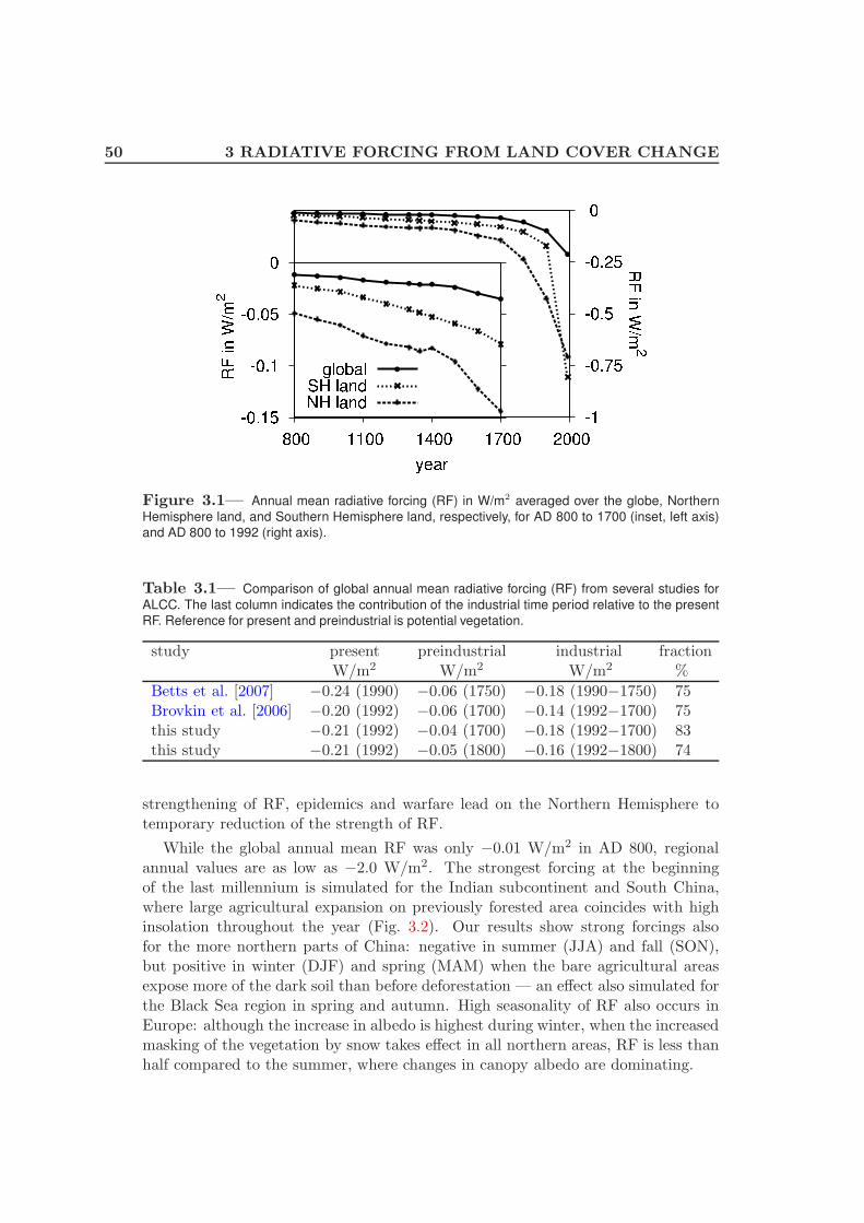
50 3 RADIATIVE FORCING FROM LAND COVER CHANGE
Figure 3.1— Annual mean radiative forcing (RF) in W/m2 averaged over the globe, Northern
Hemisphere land, and Southern Hemisphere land, respectively, for AD 800 to 1700 (inset, left axis)
and AD 800 to 1992 (right axis).
Table 3.1— Comparison of global annual mean radiative forcing (RF) from several studies for
ALCC. The last column indicates the contribution of the industrial time period relative to the present
RF. Reference for present and preindustrial is potential vegetation.
study present preindustrial industrial fractionW/m2 W/m2 W/m2 %
Betts et al. [2007] −0.24 (1990) −0.06 (1750) −0.18 (1990−1750) 75Brovkin et al. [2006] −0.20 (1992) −0.06 (1700) −0.14 (1992−1700) 75this study −0.21 (1992) −0.04 (1700) −0.18 (1992−1700) 83this study −0.21 (1992) −0.05 (1800) −0.16 (1992−1800) 74
strengthening of RF, epidemics and warfare lead on the Northern Hemisphere totemporary reduction of the strength of RF.
While the global annual mean RF was only −0.01 W/m2 in AD 800, regionalannual values are as low as −2.0 W/m2. The strongest forcing at the beginningof the last millennium is simulated for the Indian subcontinent and South China,where large agricultural expansion on previously forested area coincides with highinsolation throughout the year (Fig. 3.2). Our results show strong forcings alsofor the more northern parts of China: negative in summer (JJA) and fall (SON),but positive in winter (DJF) and spring (MAM) when the bare agricultural areasexpose more of the dark soil than before deforestation — an effect also simulated forthe Black Sea region in spring and autumn. High seasonality of RF also occurs inEurope: although the increase in albedo is highest during winter, when the increasedmasking of the vegetation by snow takes effect in all northern areas, RF is less thanhalf compared to the summer, where changes in canopy albedo are dominating.
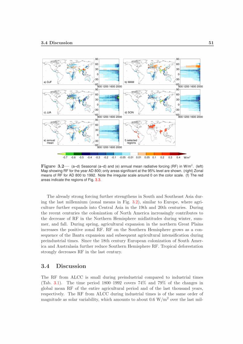
3.4 Discussion 51
a) DJF
90
60
30
0
-30
-60800 1200 1600 2000
b) MAM
90
60
30
0
-30
-60800 1200 1600 2000
c) JJA
90
60
30
0
-30
-60800 1200 1600 2000
d) SON
90
60
30
0
-30
-60800 1200 1600 2000
e) annualmean
90
60
30
0
-30
-60800 1200 1600 2000
f) selectedregions
-0.7 -0.6 -0.5 -0.4 -0.3 -0.2 -0.1 -0.05 -0.01 0.01 0.05 0.1 0.2 0.3 0.4 W/m2
Figure 3.2— (a–d) Seasonal (a–d) and (e) annual mean radiative forcing (RF) in W/m2. (left)
Map showing RF for the year AD 800; only areas significant at the 95% level are shown. (right) Zonal
means of RF for AD 800 to 1992. Note the irregular scale around 0 on the color scale. (f) The red
areas indicate the regions of Fig. 3.3.
The already strong forcing further strengthens in South and Southeast Asia dur-ing the last millennium (zonal means in Fig. 3.2), similar to Europe, where agri-culture further expands into Central Asia in the 19th and 20th centuries. Duringthe recent centuries the colonization of North America increasingly contributes tothe decrease of RF in the Northern Hemisphere midlatitudes during winter, sum-mer, and fall. During spring, agricultural expansion in the northern Great Plainsincreases the positive zonal RF. RF on the Southern Hemisphere grows as a con-sequence of the Bantu expansion and subsequent agricultural intensification duringpreindustrial times. Since the 18th century European colonization of South Amer-ica and Australasia further reduce Southern Hemisphere RF. Tropical deforestationstrongly decreases RF in the last century.
3.4 Discussion
The RF from ALCC is small during preindustrial compared to industrial times(Tab. 3.1). The time period 1800–1992 covers 74% and 79% of the changes inglobal mean RF of the entire agricultural period and of the last thousand years,respectively. The RF from ALCC during industrial times is of the same order ofmagnitude as solar variability, which amounts to about 0.6 W/m2 over the last mil-

52 3 RADIATIVE FORCING FROM LAND COVER CHANGE
lennium, causing temperature variabilities in the order of 0.2 K [Crowley, 2000].The changes of RF from ALCC during the preindustrial times of the last millen-nium are one order of magnitude smaller than solar variability, and two orders incomparison with volcanic forcing, as large eruptions typically cause a RF of sev-eral W/m2 [Crowley, 2000]. ALCC, however, differs from the natural forcings intwo respects: First, ALCC constitutes a rather permanent forcing, unlike volcaniceruptions. By its persistence over centuries even a small forcing as preindustrialALCC may significantly affect the long-term energy balance. This notion has beensupported by previous studies attributing Northern Hemisphere cooling to ALCC[e.g. Govindasamy et al., 2001, Goosse et al., 2006] and will be discussed in thefollowing. Second, ALCC constitutes a highly heterogeneous forcing and opposingeffects in time and space tend to counterbalance on the global and annual mean sothat significant regional effects may be masked. Betts et al. [2007], for example,find a cooling of 1–2 K in winter and spring over northern midlatitude agriculturalregions as a consequence of ALCC-induced albedo changes. In this study, annualmean values as low as −2.0 W/m2 are simulated for South Asia in AD 800, whichare in the same order of magnitude, though opposite in sign, as the greenhouse gasforcing in present times. Despite small mean values of RF, ALCC may thus havealtered regional climate already a thousand years ago. Specific regions further ex-hibit very distinct histories of agricultural development with partly abrupt changesin RF, as will be illustrated later.
The negative RF in the northern midlatitudes during fall, winter, and most no-tably summer must be expected to have a cooling effect in accordance with studies bye.g. Betts et al. [2007]. This albedo change has also been suggested by Govindasamyet al. [2001] as the key player in explaining the Northern Hemisphere cooling of about0.25 K between AD 1000 and 1900 reconstructed from climate proxies [Mann andBradley, 1999]. In our study, the RF of the Northern Hemisphere decreases by0.11 W/m2 during this period, as compared to a RF of 0.28 W/m2 by Govindasamyet al. [2001]. In contrast to their study, our findings thus suggest that ALCC duringthis time period cannot be the major cause for the cooling. A main difference isthat we apply a detailed land cover reconstruction, while Govindasamy et al. [2001]assume present-day land cover for the year 1900 and potential vegetation in AD 1000so that deforestation is significantly overestimated.
Ruddiman [2007] suggests that epidemics such as the bubonic plague in the 14thcentury Europe and the mass mortality in the Americas after European arrival hadlowered atmospheric CO2 concentrations, because agricultural land was abandonedin the course of the many deaths and was regrown by natural vegetation. In Fig. 3.3 aand b we show the RF in these two regions between AD 800 and 1700, indicatingthe effect of the surface albedo changes associated with the two epidemics. Forestregrows on about 0.18 million km2 in Europe and weakens the RF by about onethird or 0.08 W/m2 in the indicated area within just one century. In the region ofthe high cultures of Meso- and South America the RF loses strength from −0.23 to−0.09 W/m2 between AD 1500 and 1600. Similarly, warfare may affect land coverby their impact on population distribution; the Mongol invasion and the upheavals
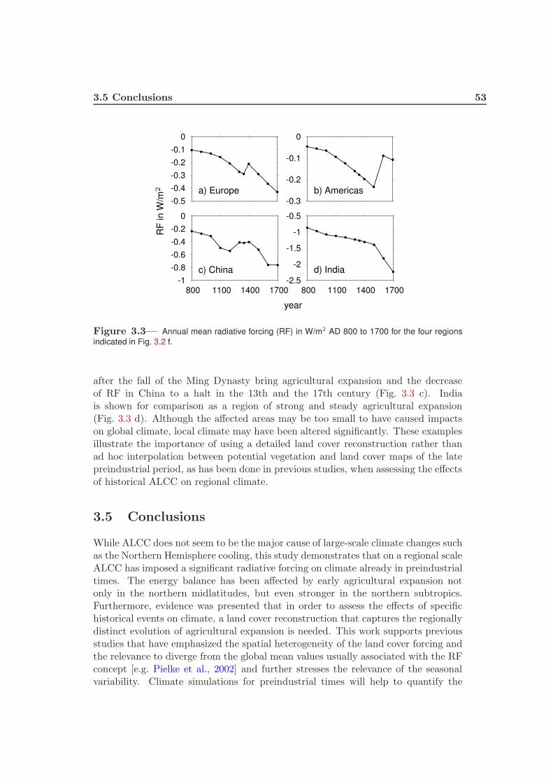
3.5 Conclusions 53
-0.5
-0.4
-0.3
-0.2
-0.1
0
800 1100 1400 1700
a) Europe-0.3
-0.2
-0.1
0
800 1100 1400 1700
b) Americas
-1
-0.8
-0.6
-0.4
-0.2
0
800 1100 1400 1700
c) China-2.5
-2
-1.5
-1
-0.5
800 1100 1400 1700
d) India
year
RF
inW
/m2
Figure 3.3— Annual mean radiative forcing (RF) in W/m2 AD 800 to 1700 for the four regions
indicated in Fig. 3.2 f.
after the fall of the Ming Dynasty bring agricultural expansion and the decreaseof RF in China to a halt in the 13th and the 17th century (Fig. 3.3 c). Indiais shown for comparison as a region of strong and steady agricultural expansion(Fig. 3.3 d). Although the affected areas may be too small to have caused impactson global climate, local climate may have been altered significantly. These examplesillustrate the importance of using a detailed land cover reconstruction rather thanad hoc interpolation between potential vegetation and land cover maps of the latepreindustrial period, as has been done in previous studies, when assessing the effectsof historical ALCC on regional climate.
3.5 Conclusions
While ALCC does not seem to be the major cause of large-scale climate changes suchas the Northern Hemisphere cooling, this study demonstrates that on a regional scaleALCC has imposed a significant radiative forcing on climate already in preindustrialtimes. The energy balance has been affected by early agricultural expansion notonly in the northern midlatitudes, but even stronger in the northern subtropics.Furthermore, evidence was presented that in order to assess the effects of specifichistorical events on climate, a land cover reconstruction that captures the regionallydistinct evolution of agricultural expansion is needed. This work supports previousstudies that have emphasized the spatial heterogeneity of the land cover forcing andthe relevance to diverge from the global mean values usually associated with the RFconcept [e.g. Pielke et al., 2002] and further stresses the relevance of the seasonalvariability. Climate simulations for preindustrial times will help to quantify the

54 3 RADIATIVE FORCING FROM LAND COVER CHANGE
actual climate response to all biogeophysical effects of historical ALCC includingfeedbacks, and transient simulations over the last millennium should be performedto further include the evolution of land cover CO2 emissions and their impact onpreindustrial climate.

55
Chapter 4
Effects of Anthropogenic LandCover Change on the CarbonCycle of the Last Millennium
Abstract
Transient simulations are performed over the entire last millennium with a generalcirculation model that couples the atmosphere, ocean, and the land surface witha closed carbon cycle. This setup applies a high-detail reconstruction of anthro-pogenic land cover change (ALCC) as the only forcing to the climate system withtwo goals: (1) to isolate the effects of ALCC on the carbon cycle and the climateindependently of any other natural and anthropogenic disturbance and (2) to assessthe importance of preindustrial human activities. With ALCC as only forcing, theterrestrial biosphere remains a source of carbon throughout the last millennium,with a net release of 96 Gt C and an increase of atmospheric CO2 by 20 ppm. Thebiosphere-atmosphere coupling thereby leads to a restorage of 37% and 48% of theprimary emissions over the industrial and the preindustrial period, respectively. Dueto the stronger coupling flux over the preindustrial period, only 21% of the 53 GtC preindustrial emissions remain airborne. Despite the low airborne fraction, atmo-spheric CO2 rises above natural variability by late medieval times. This suggeststhat human influence on CO2 began prior to industrialization. Global mean tem-peratures, however, are not significantly altered until the strong population growthin the industrial period. Furthermore, we investigate the effects of historic eventssuch as epidemics and warfare on the carbon budget. We find that only long-lastingevents such as the Mongol invasion lead to carbon sequestration. The reason for thislimited carbon sequestration are indirect emissions from past ALCC that compen-sate carbon uptake in regrowing vegetation for several decades. Drops in ice coreCO2 are thus unlikely to be attributable to human action. Our results indicate thatclimate-carbon cycle studies for present and future centuries, which usually startfrom an equilibrium state around 1850, start from a significantly disturbed state of
56 4 LAND COVER CHANGE AND CARBON CYCLE
the carbon cycle.
4.1 Introduction
The vegetation covering the continents has a decisive influence on the climate.Through the uptake of CO2 from the atmosphere, plants play a central role in theglobal carbon cycle. Furthermore, they influence the exchange of energy, water, andmomentum between the atmosphere and the land surface. Humankind is alteringthese processes by transforming areas of natural vegetation to human use in agricul-ture, forestry, and urbanization (“anthropogenic land cover change”, ALCC). Theanthropogenic disturbance of the natural land cover has started thousands of yearsago with the expansion of agriculture, and possibly earlier with hunters and gath-erers managing woodlands for hunting and traveling. The disturbance has grownto create a human-dominated world today, as 30–50% of the Earth’s land cover aresubstantially modified by human land use — primarily by the expansion of agricul-ture [Vitousek et al., 1997]. The recognition is growing that ALCC has an impacton climate and the carbon cycle and needs thorough investigation to understandits pathways of disturbance, its past and future effects, as well as its potential tomitigate climate change [Barker et al., 2007, Denman et al., 2007]. Consequently,land-use modules including carbon cycling are being developed for many terres-trial biosphere or climate models [e.g., McGuire et al., 2001, Strassmann et al.,2008]. They ideally calculate all fluxes endogenously and coupled to the atmosphereand ocean to allow for, e.g., a closed, interactive carbon cycle including biosphere-atmosphere feedbacks. Eventually, the recommendation was given to supply ALCCas spatially explicit information to the climate projections of the next report of theIntergovernmental Panel on Climate Change [Moss et al., 2008].
The influence of vegetation cover and ALCC on the climate is commonly dividedinto biogeophysical and biogeochemical mechanisms. The first include all modifica-tions of the physical properties of the land surface such as albedo, roughness, andevapotranspiration. Modeling studies suggest that at mid- and high latitudes theincrease of albedo is the dominant biogeophysical process of ALCC. Albedo increasesas a consequence of deforestation — due to the higher snow-free albedo of non-forestvegetation as well as the snow masking effect of forest [Bonan et al., 1992] — andgenerally induces a cooling, possibly enforced by the sea ice-albedo feedback [e.g.,Betts, 2001, Claussen et al., 2001, Bounoua et al., 2002]. In the tropics, the re-duction of evapotranspiration following deforestation leads to a loss of evaporativecooling and counteracts the albedo effect. Tropical deforestation can thus lead toa local warming [e.g., Claussen et al., 2001, Bounoua et al., 2002, DeFries et al.,2002], although its effects on the extra-tropics may be a cooling from the reducedatmospheric content of water vapor acting as a greenhouse gas [e.g., Sitch et al.,2005].
Probably the most important biogeochemical mechanism of ALCC is the influenceon the carbon cycle, and the associated impact on the global CO2 concentration.
4.1 Introduction 57
Altering atmospheric CO2, ALCC modifies the Earth’s energy balance and thusclimate. ALCC constitutes a source of emissions mainly from the loss of terres-trial biomass. About one third of the anthropogenic CO2 emissions over the last150 years are estimated to be the direct consequence of ALCC [Houghton, 2003].Counteracting the emissions is an increased carbon uptake by both natural andagricultural vegetation, the so-called “residual land sink” [Denman et al., 2007]. Itscauses are not well specified and assumed to be, among others, the fertilizing effectof increased atmospheric CO2, nitrogen deposition, recovery from past disturbances,and climate change [Schimel et al., 2001, and references therein]. The net effect isthat the terrestrial biosphere has turned from a source to a sink during the recentdecades, thus mitigating anthropogenic greenhouse gas emissions. All these carbonfluxes, however, are very uncertain. The uncertainty range assigned to estimates ofALCC emissions is about ±70% even for the last — best-documented — decades,and propagates to the carbon sink term [Denman et al., 2007]. Difficulties in quanti-fying and locating ALCC are only one problem beside gaps in process understandingand model differences [McGuire et al., 2001]. Further complexity is added by theinteraction of biogeophysical and biogeochemical effects and the two-way couplingof the carbon cycle and the climate.
Primary emissions by ALCC have first been estimated either by simple book-keeping approaches [Houghton et al., 1983] or by spatially explicit simulations ofcarbon stocks for different time slices by process-oriented models [DeFries et al.,1999, Olofsson and Hickler, 2008]. Primary emissions are now increasingly derivedfrom transient studies, though only for the last three centuries. In these studies,carbon loss, uptake, and the net effect of ALCC on the carbon cycle are simulated.Climate and CO2 fields may either be prescribed in these simulations [McGuireet al., 2001, Jain and Yang, 2005], in which case no feedbacks from ALCC on theclimate are allowed; or they may be calculated interactively. The latter method hasbeen used for past and future ALCC in a range of studies applying Earth systemmodels of intermediate complexity (EMICs) [Gitz and Ciais, 2003, Sitch et al., 2005,Brovkin et al., 2006, Strassmann et al., 2008]. Recently, second-order effects ofALCC were identified, such as the loss of carbon sink capacity by replacing forestswith agricultural land [Gitz and Ciais, 2003]. Several studies have focused only onthe net effect of potential ALCC scenarios and the resulting influence on climate ofthe biogeochemical effects in comparison to the biogeophysical ones [e.g., Claussenet al., 2001, Brovkin et al., 2004].
In the present study, we apply a general circulation model (GCM) for the atmo-sphere and the ocean coupled to a land surface scheme, considering both biogeophys-ical and biogeochemical effects of ALCC. Our model includes a closed carbon cycle(land, ocean, atmosphere) that evolves interactively with the climate. Feedbacksbetween the carbon cycle and the climate are thus included in the simulations.We distinguish between source and sink terms and identify further sub-processesof biosphere-atmosphere carbon exchange. A detailed reconstruction of ALCC isapplied that indicates areas of cropland, pasture, and natural vegetation for eachyear since AD 800 [Pongratz et al., 2008b], which allows us to quantify the effects
58 4 LAND COVER CHANGE AND CARBON CYCLE
of ALCC transiently over history. To our knowledge, the combination of method,data, and the length of the simulated time period makes this study the first to assessthe effects of ALCC on the carbon cycle and the climate in such detail.
We do not try to simulate a realistic climate evolution as influenced by all naturaland anthropogenic forcings, but we try to isolate the impact of ALCC on climateby allowing ALCC as the only forcing to the carbon cycle and climate system.Anthropogenic carbon emissions from fossil-fuel burning and cement production arethe most important driver of CO2 and climate change today, but did not growsignificantly larger than ALCC emissions until the 1930s [Houghton, 2003, Marlandet al., 2008], and played no role in the preindustrial period. For the preindustrialera, our model results can therefore be expected to represent most of the real impactof human activity. The studies by DeFries et al. [1999], Olofsson and Hickler [2008],Ruddiman [2003, 2007] clearly indicate that significant amounts of carbon werealready released in the preindustrial period, but estimates range from 48–320 GtC. The net effect of preindustrial ALCC is even more disputed, ranging from akey climate forcing [Ruddiman, 2007] to a very small one [Joos et al., 2004]. Ithas also been suggested that historic events such as warfare and epidemics alteredatmospheric CO2 via their impact on agricultural extent [Ruddiman, 2007], but athorough investigation has not been undertaken since, until recently, no spatiallyexplicit information on the actual changes of vegetation distribution existed. Ourstudy assesses the effects of historic events over the last millennium and gives newestimates for associated carbon source and sink terms. Including also the carboncycle in the ocean, we can estimate the amount of carbon that remains in theatmosphere and address the question whether an anthropogenic influence on thecarbon cycle, and finally climate, has existed prior to the industrialization.
4.2 Methods
4.2.1 Model
The atmosphere/ocean general circulation model (AOGCM) consists of ECHAM5[Roeckner et al., 2003] at T31 (approximately 4 degree) resolution with 19 verticallevels representing the atmosphere, and MPI-OM [Marsland et al., 2003] at 3 de-gree resolution with 40 vertical levels representing the ocean. The two models arecoupled daily without flux correction. The carbon cycle model comprises the oceanbiogeochemistry model HAMOCC5 [Wetzel et al., 2005] and the modular land sur-face scheme JSBACH [Raddatz et al., 2007]. HAMOCC5 simulates inorganic carbonchemistry as well as phyto- and zooplankton dynamics in dependence of tempera-ture, solar radiation, and nutrients. It also considers the buildup of detritus, itssinking, remineralization, and sedimentation. JSBACH distinguishes 12 plant func-tional types (PFTs), including one crop type, which differ with respect to theirphenology, morphological and photosynthetic parameters. Their fractional coverageof each grid cell is prescribed from maps annually. For each PFT, the storage oforganic carbon on land occurs in five pools: living tissue (“green”), woody material

4.2 Methods 59
(“wood”), and a pool storing sugar and starches (“reserve”) for the vegetation car-bon, and two soil carbon pools with a fast (about 1.5 years) and a slow turnoverrate (about 150 years).
For this study ALCC was implemented in JSBACH as follows: The change in thecover fractions of PFTs is prescribed from the maps described below and linearlyinterpolated from annual changes to a daily timestep. With changes in the coverfractions, carbon is relocated between the pools. The vegetation carbon of PFTswith decreasing area is either directly released to the atmosphere, or relocated tothe two soil pools. Carbon release directly to the atmosphere happens, e.g., whenforest is cleared by fire, and a fraction of 50% of the vegetation carbon is chosenin this study as flux to the atmosphere. The choice of this value is not critical forthe present analysis: The timescale of our study is multi-centennial and thus largerthan the slowest turnover rate of the carbon pools, so that all vegetation carbonlost is eventually transferred to the atmosphere. The amount of ALCC carbon perm2 and day directly released to the atmosphere from the three vegetation pools iscalculated as
F⊲A =∑
i∈ a−
(coldi − cnew
i ) (4.1)
·(fG⊲ACG,i + fW⊲ACW,i + fR⊲ACR,i) ,
where fG⊲A, fW⊲A, and fR⊲A denote the fractions of carbon released to the atmo-sphere due to ALCC for the three vegetation carbon pools (green, wood, and reserve,respectively). cold
i − cnewi denotes the daily change in cover fraction of the i-th PFT
that loses area (a−) due to ALCC, and CG,i, CW,i, and CR,i denote the carbondensities of the three vegetation pools. For the relocation of vegetation carbon tothe two soil pools, the carbon from the green and reserve pools is transferred to thefast soil pool in each grid cell, while the carbon from the wood pool is transferredto the slow soil pool. The long decay time of the slow soil pool implicitly includesthe storage of carbon in long-term human use. The ALCC carbon fluxes to the fastand slow pool are calculated as
F⊲F =∑
i∈ a−
(coldi − cnew
i ) (4.2)
· [(1 − fG⊲A)CG,i + (1 − fR⊲A)CR,i]
F⊲S =∑
i∈ a−
(coldi − cnew
i )(1 − fW⊲A)CW,i . (4.3)
Vegetation carbon is therefore lost from a PFT only due to the decrease of its area,while its carbon densities are unaffected. The carbon lost is then transferred tothe respective soil carbon pools of the expanding PFTs, distributed proportionallyto their new cover fractions, and the PFT carbon densities adjusted accordingly.This scheme describes the temporal evolution of land carbon storage for agriculturalexpansion as well as abandonment consistently.

60 4 LAND COVER CHANGE AND CARBON CYCLE
4.2.2 ALCC data
As ALCC forcing, the reconstruction of global agricultural areas and land cover byPongratz et al. [2008b] is applied. It contains fractional maps of 14 vegetation typesat an annual timestep and a spatial resolution of 0.5 degree. The agricultural typesconsidered are cropland, C3, and C4 pasture. The reconstruction merges publishedmaps of agriculture from AD 1700 to 1992 and a population-based approach toquantify agriculture for each country for the time period AD 800 to 1700. With thisapproach the general expansion of agriculture is captured as well as specific historicevents, such as epidemics and wars, that are likely to have caused abandonment ofagricultural area in certain regions due to their impact on population numbers. Theuncertainty associated with the chosen approach, with respect to the uncertaintyof population data and of agrotechnological development, was assessed in two ad-ditional datasets for AD 800 to 1700, which indicate the upper and lower range ofpossible agricultural extent.
A map of potential vegetation with 11 PFTs was used as background to theagricultural reconstruction with different allocation rules for cropland and pasture.Most previous studies that included pasture interpreted the expansion of pastureas deforestation or reduced all natural vegetation equally, not taking into accountthat in history humans used natural grasslands for pastures rather than clearingforested area [e.g., Houghton, 1999], thus overestimating ALCC. The ALCC recon-struction applied here implemented the preferential allocation of pasture on naturalgrasslands.
ALCC other than caused by the change in agricultural extent, e.g., shifting cul-tivation and wood harvest on areas that are not subsequently used for agriculture,is not taken into account in this study. However, forestry for wood production is ex-pected to have only a small effect on the net carbon balance, as harvest in most casestends to be compensated by regrowth [Houghton, 2003]. The same effect makes thedistinction of agricultural area as either permanent or part of a system of shiftingcultivation less important. In this study, all agriculture is treated as permanent.An extension of the agricultural and land cover maps into the future follows theA1B scenario [Nakicenovic et al., 2000], superimposing changes in agricultural ex-tent from the scenario maps on the ALCC map of 1992, the last map available fromthe ALCC reconstruction.
4.2.3 Simulation protocol
The model is spun up for more than 4000 years under CH4, N2O, solar, orbital, andland cover conditions of the year AD 800 until the carbon pools are in equilibrium.The final atmospheric CO2 concentration is 281 ppm. Three simulations branch offfrom this equilibrium (Tab. 4.1): A 1300-year-long control simulation (named ctrl)keeps all forcings constant at the year AD 800 state, while two transient simulationsrun until the year 2100 applying ALCC as the only forcing (LC). The first appliesthe middle-range (best-guess) ALCC reconstruction with the aim to capture the
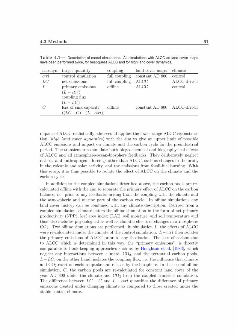
4.2 Methods 61
Table 4.1— Description of model simulations. All simulations with ALCC as land cover maps
have been performed twice, for best-guess ALCC and for high land cover dynamics.
acronym target quantity coupling land cover maps climate
ctrl control simulation full coupling constant AD 800 controlLC net emissions full coupling ALCC ALCC-drivenL primary emissions
(L − ctrl)offline ALCC control
coupling flux(L − LC)
C loss of sink capacity((LC−C)−(L−ctrl))
offline constant AD 800 ALCC-driven
impact of ALCC realistically; the second applies the lower-range ALCC reconstruc-tion (high land cover dynamics) with the aim to give an upper limit of possibleALCC emissions and impact on climate and the carbon cycle for the preindustrialperiod. The transient runs simulate both biogeochemical and biogeophysical effectsof ALCC and all atmosphere-ocean-biosphere feedbacks. They deliberately neglectnatural and anthropogenic forcings other than ALCC, such as changes in the orbit,in the volcanic and solar activity, and the emissions from fossil-fuel burning. Withthis setup, it is thus possible to isolate the effect of ALCC on the climate and thecarbon cycle.
In addition to the coupled simulations described above, the carbon pools are re-calculated offline with the aim to separate the primary effect of ALCC on the carbonbalance, i.e. prior to any feedbacks arising from the coupling with the climate andthe atmospheric and marine part of the carbon cycle. In offline simulations anyland cover history can be combined with any climate description. Derived from acoupled simulation, climate enters the offline simulation in the form of net primaryproductivity (NPP), leaf area index (LAI), soil moisture, and soil temperature andthus also includes physiological as well as climatic effects of changes in atmosphericCO2. Two offline simulations are performed: In simulation L, the effects of ALCCwere re-calculated under the climate of the control simulation. L− ctrl then isolatesthe primary emissions of ALCC prior to any feedbacks. The loss of carbon dueto ALCC which is determined in this way, the “primary emissions”, is directlycomparable to book-keeping approaches such as by Houghton et al. [1983], whichneglect any interactions between climate, CO2, and the terrestrial carbon pools.L−LC, on the other hand, isolates the coupling flux, i.e. the influence that climateand CO2 exert on carbon uptake and release by the biosphere. In the second offlinesimulation, C, the carbon pools are re-calculated for constant land cover of theyear AD 800 under the climate and CO2 from the coupled transient simulation.The difference between LC − C and L − ctrl quantifies the difference of primaryemissions created under changing climate as compared to those created under thestable control climate.

62 4 LAND COVER CHANGE AND CARBON CYCLE
-100
-50
0
50
100
150
200
800 1000 1200 1400 1600 1800 2000
cum
ula
tive c
arb
on f
luxes (
Gt
C)
year
net emissions (ctrl−LC)primary emissions (ctrl−L)direct emissionsindirect emissionscoupling flux (L−LC)
Figure 4.1— Global land-atmosphere carbon fluxes, cumulative since AD 800. Positive values
indicate release to the atmosphere. Thick lines are results for the best-guess ALCC reconstruction,
thin lines for the high land cover dynamics. The shaded areas split up the best-guess primary emis-
sions into direct (light) and indirect (dark) emissions. Simulations ctrl, L, LC as explained in Tab. 4.1.
Values are 10-years running means.
4.3 Primary emissions and carbon cycle feedback
4.3.1 Overview
With ALCC as only forcing, the land biosphere remains a net source of carbonthroughout the last millennium (Fig. 4.1). It loses 96 Gt C between AD 800 and2000 (see Tab. 4.2 for the preindustrial, industrial, and future period). This resultsfrom a loss of vegetation carbon only partly offset by a gain in soil carbon, similaras in previous studies [e.g., Jain and Yang, 2005] (Fig. 4.2, LC − ctrl). Primaryemissions are significantly higher than the net emissions, with 161 Gt C. The differ-ence of 65 Gt C is the consequence of the coupling flux: The primary emissions alterclimate and increase atmospheric CO2 concentration (see Sec. 4.4.1). These changesenhance carbon uptake by the biosphere, in particular via CO2 fertilization. As aconsequence, 40% of the primary emissions over the last millennium are buffered bythe biosphere.
4.3.2 Spatial patterns
The spatial distribution of the primary emissions, the coupling flux and the netemissions are shown separately for the preindustrial (AD 800–1850), the industrial(1850–2000), and the future (2000–2100) period in Fig. 4.3. The maps for the netemissions contrast clearly the regions where agricultural expansion was strong duringthe respective time period and emissions are higher than the terrestrial sink, andthose regions where carbon uptake from the coupling flux is stronger, usually theremaining pristine regions. In the preindustrial period, emissions arise primarily
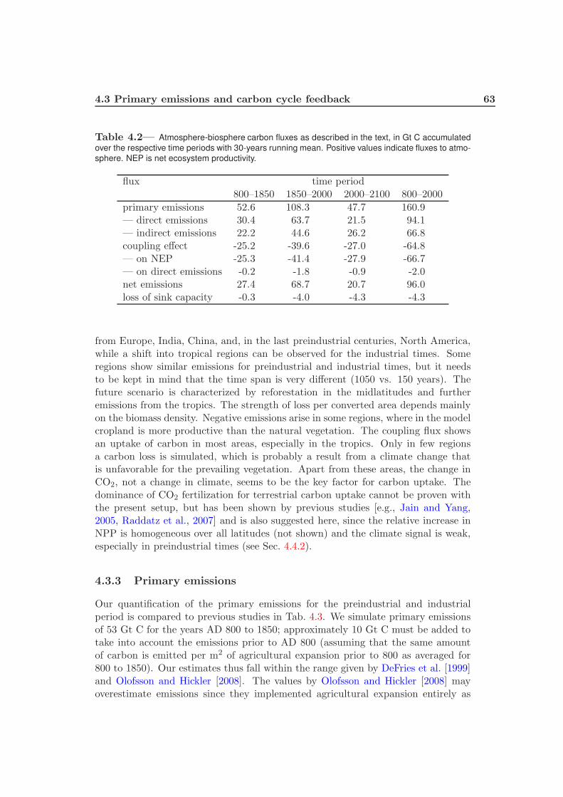
4.3 Primary emissions and carbon cycle feedback 63
Table 4.2— Atmosphere-biosphere carbon fluxes as described in the text, in Gt C accumulated
over the respective time periods with 30-years running mean. Positive values indicate fluxes to atmo-
sphere. NEP is net ecosystem productivity.
flux time period800–1850 1850–2000 2000–2100 800–2000
primary emissions 52.6 108.3 47.7 160.9— direct emissions 30.4 63.7 21.5 94.1— indirect emissions 22.2 44.6 26.2 66.8coupling effect -25.2 -39.6 -27.0 -64.8— on NEP -25.3 -41.4 -27.9 -66.7— on direct emissions -0.2 -1.8 -0.9 -2.0net emissions 27.4 68.7 20.7 96.0loss of sink capacity -0.3 -4.0 -4.3 -4.3
from Europe, India, China, and, in the last preindustrial centuries, North America,while a shift into tropical regions can be observed for the industrial times. Someregions show similar emissions for preindustrial and industrial times, but it needsto be kept in mind that the time span is very different (1050 vs. 150 years). Thefuture scenario is characterized by reforestation in the midlatitudes and furtheremissions from the tropics. The strength of loss per converted area depends mainlyon the biomass density. Negative emissions arise in some regions, where in the modelcropland is more productive than the natural vegetation. The coupling flux showsan uptake of carbon in most areas, especially in the tropics. Only in few regionsa carbon loss is simulated, which is probably a result from a climate change thatis unfavorable for the prevailing vegetation. Apart from these areas, the change inCO2, not a change in climate, seems to be the key factor for carbon uptake. Thedominance of CO2 fertilization for terrestrial carbon uptake cannot be proven withthe present setup, but has been shown by previous studies [e.g., Jain and Yang,2005, Raddatz et al., 2007] and is also suggested here, since the relative increase inNPP is homogeneous over all latitudes (not shown) and the climate signal is weak,especially in preindustrial times (see Sec. 4.4.2).
4.3.3 Primary emissions
Our quantification of the primary emissions for the preindustrial and industrialperiod is compared to previous studies in Tab. 4.3. We simulate primary emissionsof 53 Gt C for the years AD 800 to 1850; approximately 10 Gt C must be added totake into account the emissions prior to AD 800 (assuming that the same amountof carbon is emitted per m2 of agricultural expansion prior to 800 as averaged for800 to 1850). Our estimates thus fall within the range given by DeFries et al. [1999]and Olofsson and Hickler [2008]. The values by Olofsson and Hickler [2008] mayoverestimate emissions since they implemented agricultural expansion entirely as
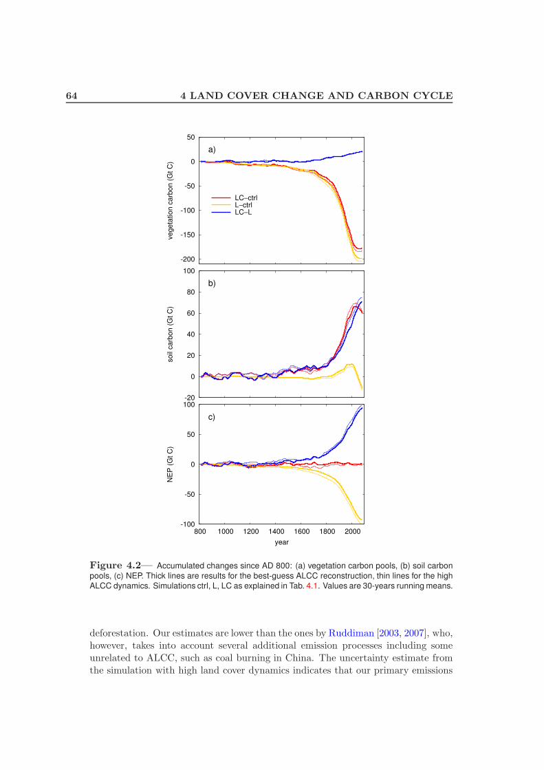
64 4 LAND COVER CHANGE AND CARBON CYCLE
-200
-150
-100
-50
0
50
ve
ge
tatio
n c
arb
on
(G
t C
)
LC−ctrlL−ctrlLC−L
a)
-20
0
20
40
60
80
100
so
il ca
rbo
n (
Gt
C)
b)
-100
-50
0
50
100
800 1000 1200 1400 1600 1800 2000
NE
P (
Gt
C)
year
c)
Figure 4.2— Accumulated changes since AD 800: (a) vegetation carbon pools, (b) soil carbon
pools, (c) NEP. Thick lines are results for the best-guess ALCC reconstruction, thin lines for the high
ALCC dynamics. Simulations ctrl, L, LC as explained in Tab. 4.1. Values are 30-years running means.
deforestation. Our estimates are lower than the ones by Ruddiman [2003, 2007], who,however, takes into account several additional emission processes including someunrelated to ALCC, such as coal burning in China. The uncertainty estimate fromthe simulation with high land cover dynamics indicates that our primary emissions
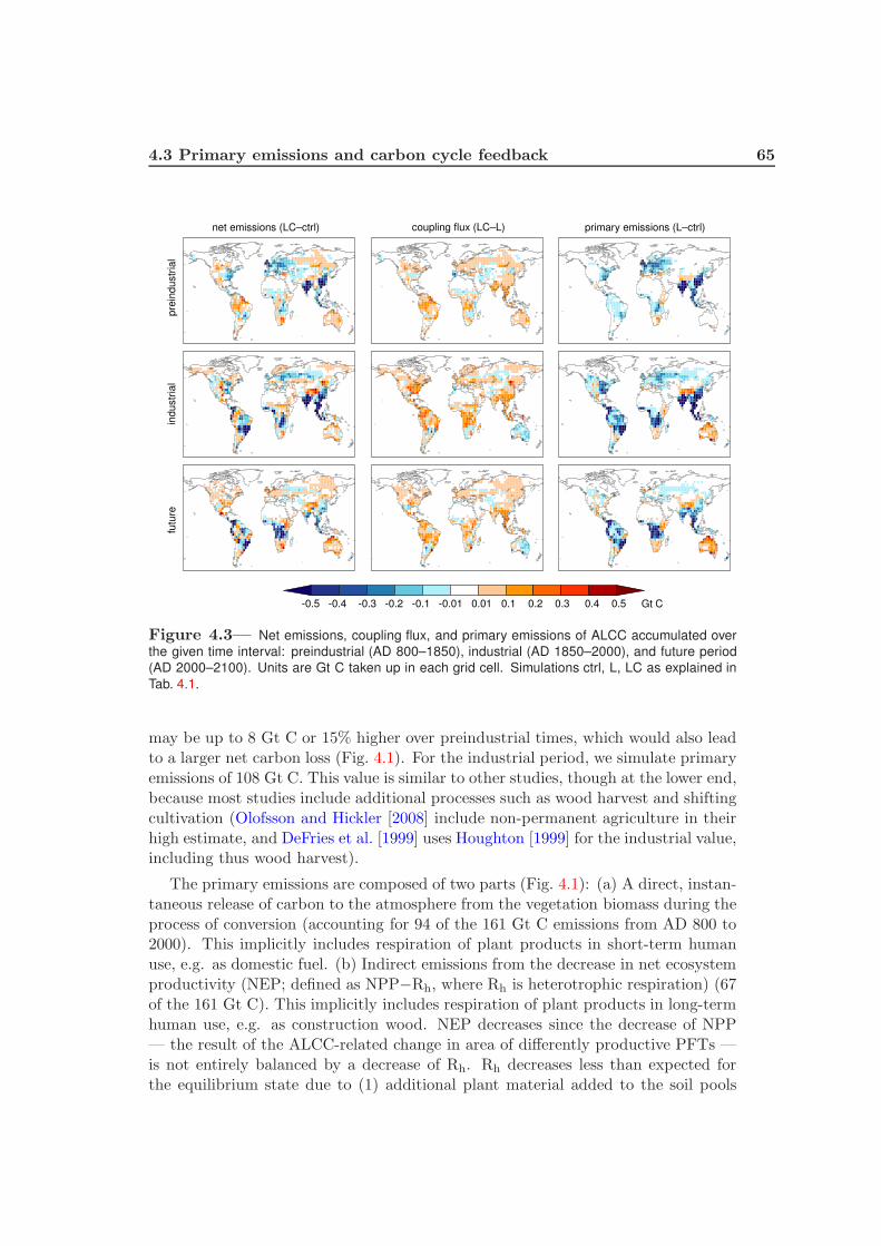
4.3 Primary emissions and carbon cycle feedback 65
-0.5 -0.4 -0.3 -0.2 -0.1 -0.01 0.01 0.1 0.2 0.3 0.4 0.5 Gt C
primary emissions (L–ctrl)coupling flux (LC–L)net emissions (LC–ctrl)
futu
rein
dustr
ial
pre
industr
ial
Figure 4.3— Net emissions, coupling flux, and primary emissions of ALCC accumulated over
the given time interval: preindustrial (AD 800–1850), industrial (AD 1850–2000), and future period
(AD 2000–2100). Units are Gt C taken up in each grid cell. Simulations ctrl, L, LC as explained in
Tab. 4.1.
may be up to 8 Gt C or 15% higher over preindustrial times, which would also leadto a larger net carbon loss (Fig. 4.1). For the industrial period, we simulate primaryemissions of 108 Gt C. This value is similar to other studies, though at the lower end,because most studies include additional processes such as wood harvest and shiftingcultivation (Olofsson and Hickler [2008] include non-permanent agriculture in theirhigh estimate, and DeFries et al. [1999] uses Houghton [1999] for the industrial value,including thus wood harvest).
The primary emissions are composed of two parts (Fig. 4.1): (a) A direct, instan-taneous release of carbon to the atmosphere from the vegetation biomass during theprocess of conversion (accounting for 94 of the 161 Gt C emissions from AD 800 to2000). This implicitly includes respiration of plant products in short-term humanuse, e.g. as domestic fuel. (b) Indirect emissions from the decrease in net ecosystemproductivity (NEP; defined as NPP−Rh, where Rh is heterotrophic respiration) (67of the 161 Gt C). This implicitly includes respiration of plant products in long-termhuman use, e.g. as construction wood. NEP decreases since the decrease of NPP— the result of the ALCC-related change in area of differently productive PFTs —is not entirely balanced by a decrease of Rh. Rh decreases less than expected forthe equilibrium state due to (1) additional plant material added to the soil pools
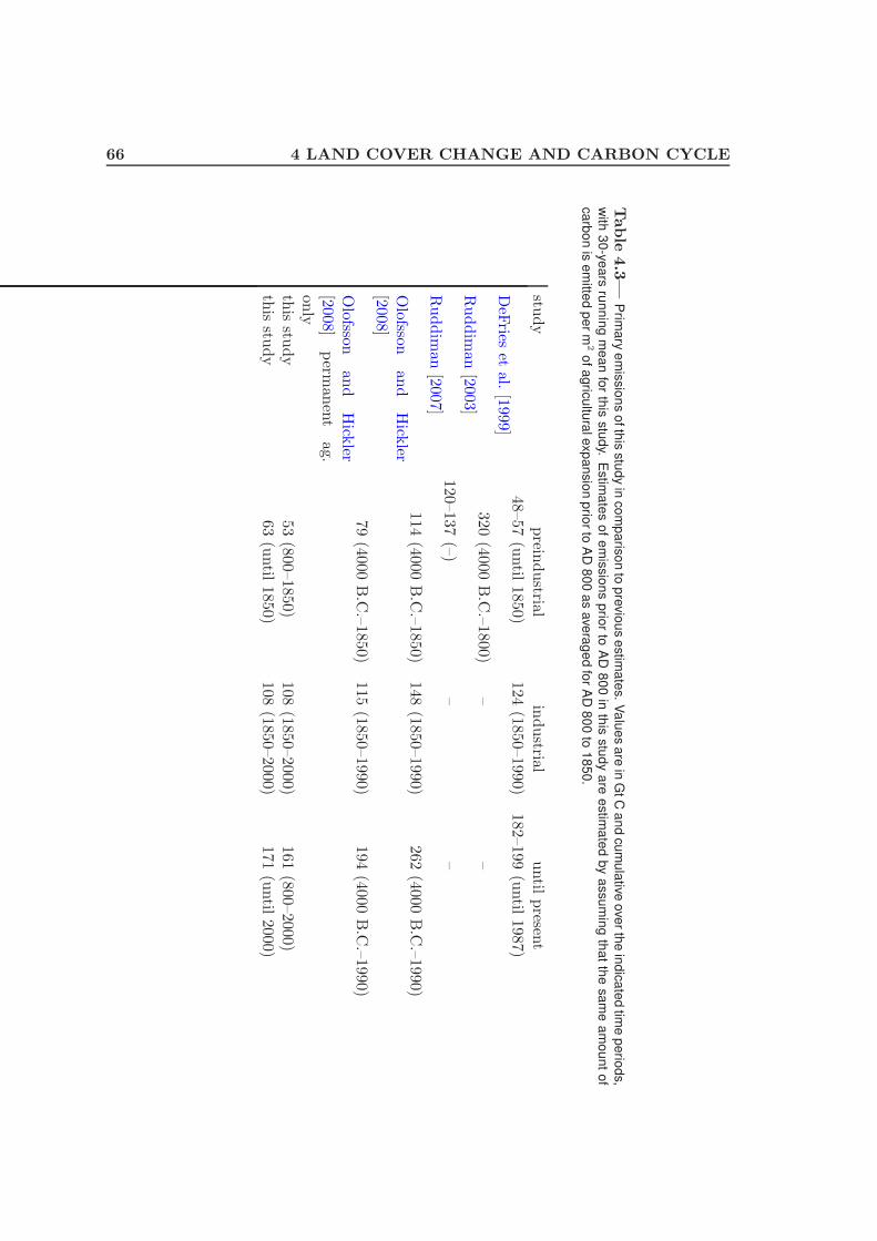
66 4 LAND COVER CHANGE AND CARBON CYCLE
Table
4.3
—P
rima
rye
mis
sio
ns
ofth
isstu
dy
inco
mp
aris
on
top
revio
us
estim
ate
s.
Va
lue
sa
rein
GtC
an
dcu
mu
lative
ove
rth
ein
dic
ate
dtim
ep
erio
ds,
with
30
-ye
ars
run
nin
gm
ea
nfo
rth
isstu
dy.
Estim
ate
so
fe
mis
sio
ns
prio
rto
AD
80
0in
this
stu
dy
are
estim
ate
dby
assu
min
gth
at
the
sa
me
am
ou
nt
of
ca
rbo
nis
em
itted
pe
rm
2o
fa
gric
ultu
rale
xp
an
sio
np
rior
toA
D8
00
as
ave
rag
ed
for
AD
80
0to
18
50
.
study
prein
dustrial
industrial
until
presen
t
DeF
rieset
al.[1999]
48–57(u
ntil
1850)124
(1850–1990)182–199
(until
1987)
Ruddim
an[2003]
320(4000
B.C
.–1800)–
–
Ruddim
an[2007]
120–137(–)
––
Olofsson
and
Hick
ler[2008]
114(4000
B.C
.–1850)148
(1850–1990)262
(4000B
.C.–1990)
Olofsson
and
Hick
ler[2008]
perm
anen
tag.
only
79(4000
B.C
.–1850)115
(1850–1990)194
(4000B
.C.–1990)
this
study
53(800–1850)
108(1850–2000)
161(800–2000)
this
study
63(u
ntil
1850)108
(1850–2000)171
(until
2000)

4.3 Primary emissions and carbon cycle feedback 67
-4
-2
0
2
4
-4 -2 0 2 4
Rh (
Gt C
)
NPP (Gt C)-4 -2 0 2 4
NPP (Gt C)-4 -2 0 2 4
NPP (Gt C)
a) LC–ctrl b) L–ctrl c) LC–L
Figure 4.4— Changes in soil respiration Rh over changes in net primary productivity NPP. Gray
shades indicate the time period: preindustrial (light), industrial (medium), future (dark). Simulations
ctrl, L, LC as explained in Tab. 4.1. Values are 50-years running means.
from the converted natural vegetation and (2) excess soil organic matter from pastconversions, which accumulates due to the time lag of Rh to NPP. The disequilib-rium between NPP and Rh is depicted in Fig. 4.4: Fig. 4.4 a shows the changes inthe transient coupled simulation, where both NPP and Rh increase, but no appar-ent disequilibrium occurs. The change in land cover alone, however, decreases NPPstronger than Rh (Fig. 4.4 b) due to the additional and excess soil organic matter.The disequilibrium vanishes in the future aforestation scenario. The coupled sim-ulation seems to be in balance because the disequilibrium with respect to primaryemissions is balanced by a disequilibrium with respect to the coupling flux: with al-tered climate and increased CO2 but unchanged land cover, NPP increases strongerthan Rh due to the time lag of Rh to NPP (Fig. 4.4 c). The latter disequilibriumhas been called an “intriguing possibility” by Denman et al. [2007] in the context ofa tropical forest sink.
The indirect emissions lead to an increase of soil carbon in the long term (Fig. 4.2),though this only slightly compensates the loss of vegetation carbon. The increasedtransfer of plant material to the soil pools, especially of woody parts with slowdecomposition rates, leads to “committed” future carbon emissions beyond the in-stantaneous ALCC. This committed flux becomes the dominant source of emissionsin the aforestation scenario of the future (Tab. 4.2).
4.3.4 Coupling flux
The quantitative estimates of the coupling flux in this study cannot be compareddirectly to previous studies, as those include changes in CO2 from fossil-fuel burningin addition to ALCC emissions. While those studies assume that present CO2 lies70–100 ppm over the preindustrial level, CO2 in our study rises only by 20 ppm (thusclose to the 18 ppm found by Brovkin et al. [2004] in a comparable EMIC study).In particular due to lower CO2 fertilization the coupling flux in our study is thus
68 4 LAND COVER CHANGE AND CARBON CYCLE
lower than found e.g. by Gitz and Ciais [2003], Denman et al. [2007]. In our study,the coupling flux is even too weak to turn the biosphere into a net carbon sink,indicating that the sink capacity of the biosphere as observed for the last decadescould not be achieved if atmospheric CO2 was not additionally increased by fossil-fuelburning. As described before, the coupling flux leads to carbon uptake because of anincreasing disequilibrium between NPP and heterotrophic respiration (Fig. 4.4 c).The absorbed carbon is primarily stored in the soil carbon pools (Fig. 4.2).
The coupling flux increases NEP stronger, though only marginally, than has beendetermined above as overall strength of the coupling flux from the difference in totalterrestrial carbon. The small counteracting effect is the coupling effect on the directemissions: with the coupling to the altered climate and increased CO2, more carbonis stored in the vegetation than would be under the control climate and unalteredCO2 — and more carbon is thus released in the conversion of vegetation with ALCC.This effect amounts to only 2 Gt C until 2000.
Gitz and Ciais [2003] were the first to quantify the “land-use amplifier effect”(“replaced sinks/sources” in Strassmann et al. [2008]). This denotes the effect thatALCC “acts to diminish the sink capacity of the terrestrial biosphere by decreasingthe residence time of carbon when croplands have replaced forests”. In other words,the additional biosphere sink that arises under rising CO2 is not as large as would beunder natural vegetation, because storage in woody biomass ceases (carbon turnoverrates are thus higher for cropland). Gitz and Ciais [2003] estimate that this effectmay be as high as 125 Gt C over the 21st century for the A2 scenario. Calculationof the land-use amplifier effect in our study that most closely imitates their setupis to determine the loss of NEP for LC − C. For ALCC over the industrial period,this yields 49 Gt C. This cumulative flux, however, is composed of two parts: Onlyone part is the actual loss in additional sink from increased turnover rates that isintended to be quantified. The other part are indirect emissions from past ALCC.By comparing one simulation with static to one with transient land cover, bothunder changing CO2 and climate, Gitz and Ciais [2003] implicitly include in theland-use amplifier effect the indirect emissions. In our simulation, indirect emissionsamount to 45 Gt C, derived from the changes in NEP for L − ctrl (Tab. 4.2). Theindirect emissions have to be subtracted from the 49 Gt C in order to isolate theloss of additional sink capacity, which then amounts to only 4 Gt C. The relativedifference between indirect emissions and loss of sink capacity is certainly not ashigh in the setup by Gitz and Ciais [2003] as here, since their study has a strongerincrease of CO2 by also including fossil-fuel burning, and the underlying ALCC isdifferent. Still, with its analysis of sub-fluxes, our study suggests that a significantfraction of the land-use amplifier effect results from the indirect emissions and thusfrom past ALCC, rather than from the change in current turnover rates.
4.4 Anthropogenic influence on the preindustrial carbon cycle and climate 69
4.4 Anthropogenic influence on the preindustrial car-
bon cycle and climate
During the preindustrial period, a lower fraction of the emissions remains in theatmosphere than during the industrial period (Tab. 4.4): biospheric uptake amountsto 48% of the emissions over the preindustrial period, as compared to only 37% forthe industrial, fossil-fuel-free, period in this study. The difference to the industrialperiod is even greater when a realistic industrial period is considered that includesfossil-fuel burning: then, only 26–34% of the emissions are taken up by the biosphere,because of the additional emissions from fossil-fuel combustion (Tab. 4.4). Thisdifference in strength of biospheric uptake between the industrial and preindustrialperiod is mostly the result of a stronger coupling flux in the latter. The slow andmore linear increase of emissions gives the land biosphere more time for CO2 uptake,and CO2 fertilization is more efficient at low CO2 concentrations. The relativeuptake by the ocean is almost unaffected and remains at around one third.
4.4.1 Anthropogenic contribution to Holocene CO2 increase
As a consequence of the strong buffering of primary emissions by the biosphere andthe low airborne fraction of CO2 in the preindustrial period, the simulations show anonly slow increase of atmospheric carbon content, despite significantly altered carbonpools of the ocean and the land biosphere several centuries earlier already (Fig. 4.5).Atmospheric carbon increases by 11.5 or 13.4 Gt C over the time period 800 to 1850(5 or 6 ppm) for the best-guess ALCC and high land cover dynamics, respectively.When we assume the same airborne fraction prior to AD 800 as for 800 to 1850 andcalculate the change in atmospheric carbon proportionally to agricultural expansion,ALCC prior to 800 would add roughly 2.1 or 1.1 Gt C (1 or 0.5 ppm, best-guessALCC and high land cover dynamics, respectively). If we accounted fully for thenet emissions prior to AD 800, atmospheric CO2 may have risen above naturalvariability prior to AD 800 already. However, especially the ocean uptake mustbe expected to have been even more efficient in the early period of the Holocene,both because uptake by dissolution is higher with lower CO2 release and becausecarbonate compensation gets effective at the millennial timescale [Archer et al.,1997]. It seems thus plausible to neglect these small early net emissions. In thiscase, atmospheric carbon content has not increased beyond natural variability untilthe late medieval times, when net emissions grew larger than the natural variabilityin land-atmosphere CO2 exchange (see Fig. 4.5). This happens rather independentlyof the ALCC scenario, since the largest differences between the scenarios occur onlylater with stronger population growth in the 16th and 17th century.
With an increase of atmospheric CO2 by 5–6 ppm by AD 1850, our estimates ofthe anthropogenic contribution to the Holocene rise in CO2 are similar to the onesby Ruddiman [Ruddiman, 2003, 2007]. Ruddiman suggests in his “early anthro-pogenic hypothesis” that preindustrial ALCC emissions increase CO2 by at least9 ppm — of which about half are resulting from ALCC — and are responsible, via
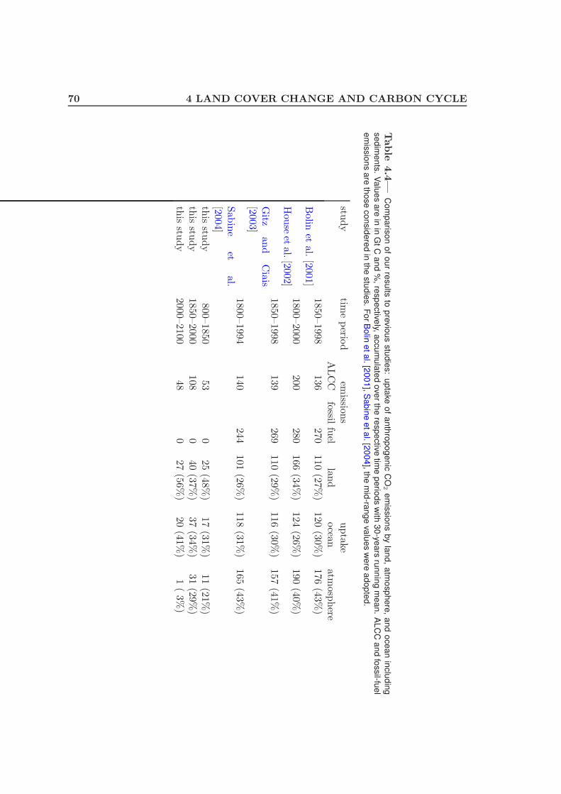
70 4 LAND COVER CHANGE AND CARBON CYCLE
Table
4.4
—C
om
pa
riso
no
fo
ur
resu
ltsto
pre
vio
us
stu
die
s:
up
take
of
an
thro
po
ge
nic
CO
2e
mis
sio
ns
by
lan
d,
atm
osp
he
re,
an
do
ce
an
inclu
din
g
se
dim
en
ts.
Va
lue
sa
rein
inG
tC
an
d%
,re
sp
ective
ly,a
ccu
mu
late
dove
rth
ere
sp
ective
time
pe
riod
sw
ith3
0-y
ea
rsru
nn
ing
me
an
.A
LC
Ca
nd
fossil-fu
el
em
issio
ns
are
tho
se
co
nsid
ere
din
the
stu
die
s.
Fo
rB
olin
eta
l.[2
00
1],
Sa
bin
ee
ta
l.[2
00
4],
the
mid
-ran
ge
valu
es
we
rea
do
pte
d.
study
time
perio
dem
issions
uptake
ALC
Cfossil
fuel
land
ocean
atmosp
here
Bolin
etal.
[2001]1850–
1998136
270110
(27%)
120(30%
)176
(43%)
Hou
seet
al.[2002]
1800–2000
200280
166(34%
)124
(26%)
190(40%
)
Gitz
and
Ciais
[2003]
1850–1998
139269
110(29%
)116
(30%)
157(41%
)
Sab
ine
etal.
[2004]
1800–1994
140244
101(26%
)118
(31%)
165(43%
)
this
study
800–1850
530
25(48%
)17
(31%)
11(21%
)th
isstu
dy
1850–2000
1080
40(37%
)37
(34%)
31(29%
)th
isstu
dy
2000–2100
480
27(56%
)20
(41%)
1(
3%)
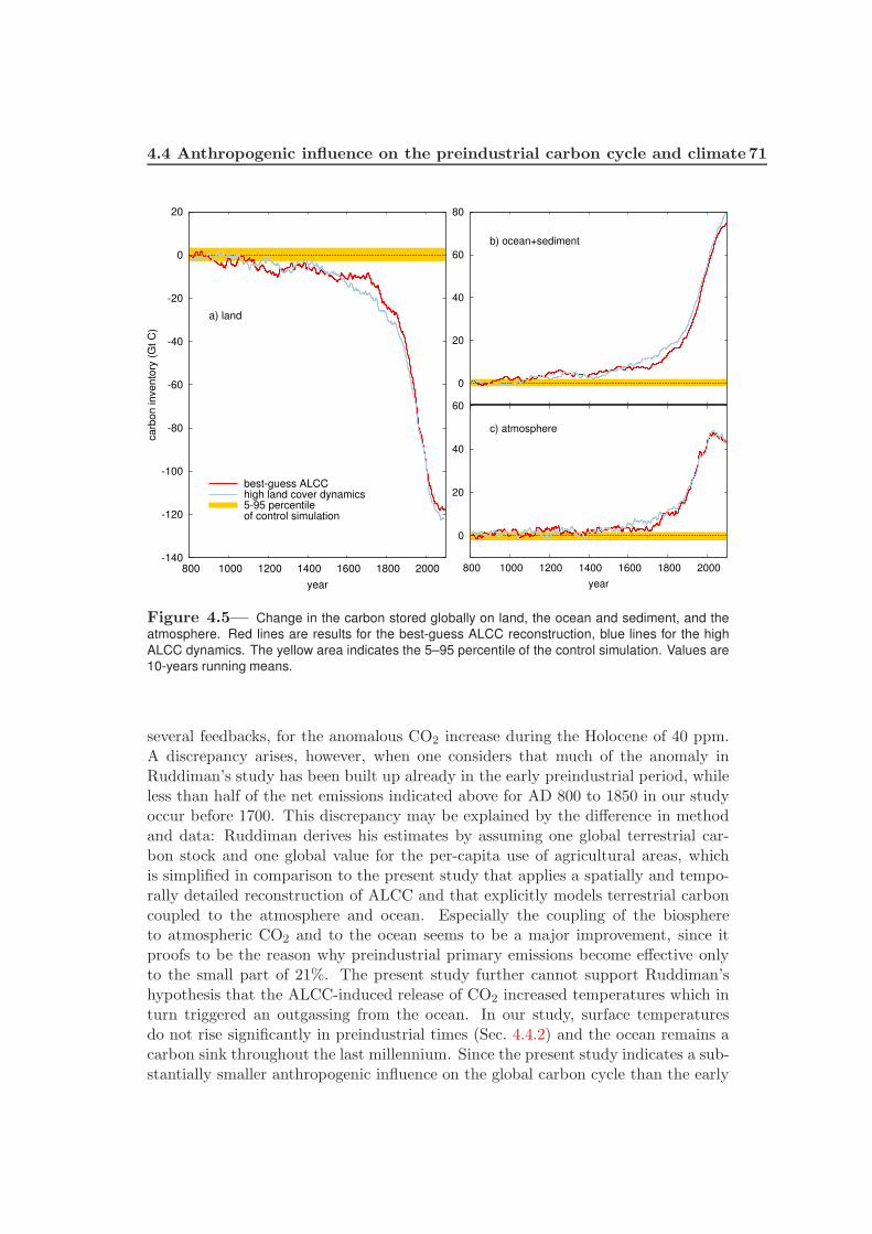
4.4 Anthropogenic influence on the preindustrial carbon cycle and climate 71
-140
-120
-100
-80
-60
-40
-20
0
20
800 1000 1200 1400 1600 1800 2000
carb
on invento
ry (
Gt C
)
year
best-guess ALCChigh land cover dynamics5-95 percentile of control simulation
a) land
0
20
40
60
800 1000 1200 1400 1600 1800 2000
year
c) atmosphere
0
20
40
60
80
800 1000 1200 1400 1600 1800 2000
b) ocean+sediment
Figure 4.5— Change in the carbon stored globally on land, the ocean and sediment, and the
atmosphere. Red lines are results for the best-guess ALCC reconstruction, blue lines for the high
ALCC dynamics. The yellow area indicates the 5–95 percentile of the control simulation. Values are
10-years running means.
several feedbacks, for the anomalous CO2 increase during the Holocene of 40 ppm.A discrepancy arises, however, when one considers that much of the anomaly inRuddiman’s study has been built up already in the early preindustrial period, whileless than half of the net emissions indicated above for AD 800 to 1850 in our studyoccur before 1700. This discrepancy may be explained by the difference in methodand data: Ruddiman derives his estimates by assuming one global terrestrial car-bon stock and one global value for the per-capita use of agricultural areas, whichis simplified in comparison to the present study that applies a spatially and tempo-rally detailed reconstruction of ALCC and that explicitly models terrestrial carboncoupled to the atmosphere and ocean. Especially the coupling of the biosphereto atmospheric CO2 and to the ocean seems to be a major improvement, since itproofs to be the reason why preindustrial primary emissions become effective onlyto the small part of 21%. The present study further cannot support Ruddiman’shypothesis that the ALCC-induced release of CO2 increased temperatures which inturn triggered an outgassing from the ocean. In our study, surface temperaturesdo not rise significantly in preindustrial times (Sec. 4.4.2) and the ocean remains acarbon sink throughout the last millennium. Since the present study indicates a sub-stantially smaller anthropogenic influence on the global carbon cycle than the early

72 4 LAND COVER CHANGE AND CARBON CYCLE
-0.1
0
0.1
0.2
0.3
800 1000 1200 1400 1600 1800 2000
tem
pera
ture
(K
)
year
best-guess ALCChigh land cover dynamics5-95 percentile of control simulation
Figure 4.6— Change in the global mean surface temperature. Red lines are results for the best-
guess ALCC reconstruction, blue lines for the high ALCC dynamics. The yellow area indicates the
5–95 percentile of the control simulation. Values are 30-years running means.
anthropogenic hypothesis, it supports studies that suggested additional reasons liketemporally limited post-glacial vegetation regrowth and carbonate compensation toexplain the CO2 anomalies (see, e.g., Claussen et al. [2005] for a discussion).
4.4.2 Effect of ALCC on global mean temperatures
A significant impact of ALCC on global mean surface temperature does not occuruntil the industrial period, when temperature starts to rise beyond the natural vari-ability (Fig. 4.6). Changes are small not only because of the low airborne fractionof CO2 and thus small greenhouse effect, but also because biogeophysical and bio-geochemical effects are counteracting each other. The anthropogenic influence onglobal mean temperature thus begins even later than on atmospheric CO2.
4.4.3 Epidemics and warfare
In addition to the hypothesis of CO2 rising anomalously during the Holocene, Rud-diman [2007] also suggests that 1–2 ppm of several sudden CO2 drops of up to8 ppm, which are reconstructed from ice core records, can be explained by epi-demics. Epidemics as well as warfare have the potential to change land cover sincenatural vegetation regrows on those agricultural areas that have been abandoned inthe course of the many deaths. Through this, previously released CO2 could againbe sequestered. The land cover reconstruction applied in this study indicates, forexample, a forest regrowth on about 0.18 million km2 as a consequence of the BlackDeath, which arrived in Europe in 1347 and killed about one third of the population[McEvedy and Jones, 1978]. Other such historic events during the last millenniumare the conquest of Middle and South America by the Europeans and both the
4.4 Anthropogenic influence on the preindustrial carbon cycle and climate 73
Mongol invasion in China and the upheavals after the fall of the Ming Dynasty.
Although the conquest of Middle and South America led to a mass mortality byepidemics as well as direct warfare (the ALCC reconstruction used in this studyassumes that 66% of the 40 million people died), this event does not imply largeareas of regrowing vegetation and alters global carbon fluxes only negligibly. Withtotal cumulative emissions of below 0.3 Gt C AD 800 to 1500 this region contributesonly 2% to global emissions; even a sequestration of the entire 0.3 Gt C would becompensated by global emissions within 6 years and could therefore not be detectedin ice core records. The reason for the few regrowing areas is mainly the assumptionof a low per-capita use of agricultural land by the native Americans, but uncertaintiesare high in this region; for details see Pongratz et al. [2008b]. Regrowth happens onlarger areas, however, during the epidemics and warfare in Europe and China.
As explained in Sec. 4.3.3, ALCC does not only imply instantaneous, but alsoindirect future emissions from changes in NEP, which arise due to the imbalanceof the soil carbon pools after ALCC. The strength of the indirect emissions of pastALCC as compared to the carbon sequestered in regrowing vegetation determineswhether farm abandonment turns a region into a carbon sink or not; transientsimulations are essential to capture this process. The Black Death and the 17thcentury upheavals in China, for example, bring emissions from NEP changes to zeroor close to it, but do not lead to negative emissions, i.e. carbon uptake from regrowth(Fig. 4.7). The amount of carbon sequestered in the regrowing vegetation is thusbalanced by the indirect emissions. For the Mongol invasion, on the other hand,NEP increases after two decades and leads to an overall carbon sink. We must thusdistinguish two kinds of events: In weak events indirect emissions from past ALCCkeep a region as carbon source despite declining agricultural area, while in strong,long-lasting events the increase of NEP with vegetation regrowth turns a region intoa carbon sink. In all events, direct emissions vanish of course during the time ofagricultural decline.
Even if a region becomes a carbon sink, the global impact of such historic eventsremains small: even during the Mongol invasion the global emission rates decrease,but do not get negative (Fig. 4.7). Other areas in the world with unperturbedagricultural expansion outdo the regional carbon uptake. This is valid, according toour simulations, even if we take into account the uncertainty of relevant parameterssuch as turnover rates of soil carbon: If we assume as a maximum estimate of carbonuptake that the entire area returns to its state of AD 800 within 100 years (theapproximate time of tree maturing) after the epidemic or war, global emissions overthe following 100 years always compensate the maximum regional regrowth. Fromthis study, it thus seems implausible that regrowth on abandoned agricultural areasfollowing epidemics and warfare, as suggested by Ruddiman [2007], caused the CO2
drops reconstructed from ice core data. Not taken into account so far, however, is theglobal coupling flux, which restores almost half of the primary emissions (Sec. 4.4).It amounts to about 12 Mt C per year averaged over 800 to 1500, and 48 Mt C peryear 1500 to 1700. These values are close to the respective minima in global primaryemissions, so that global carbon sequestration may indeed temporarily occur. The
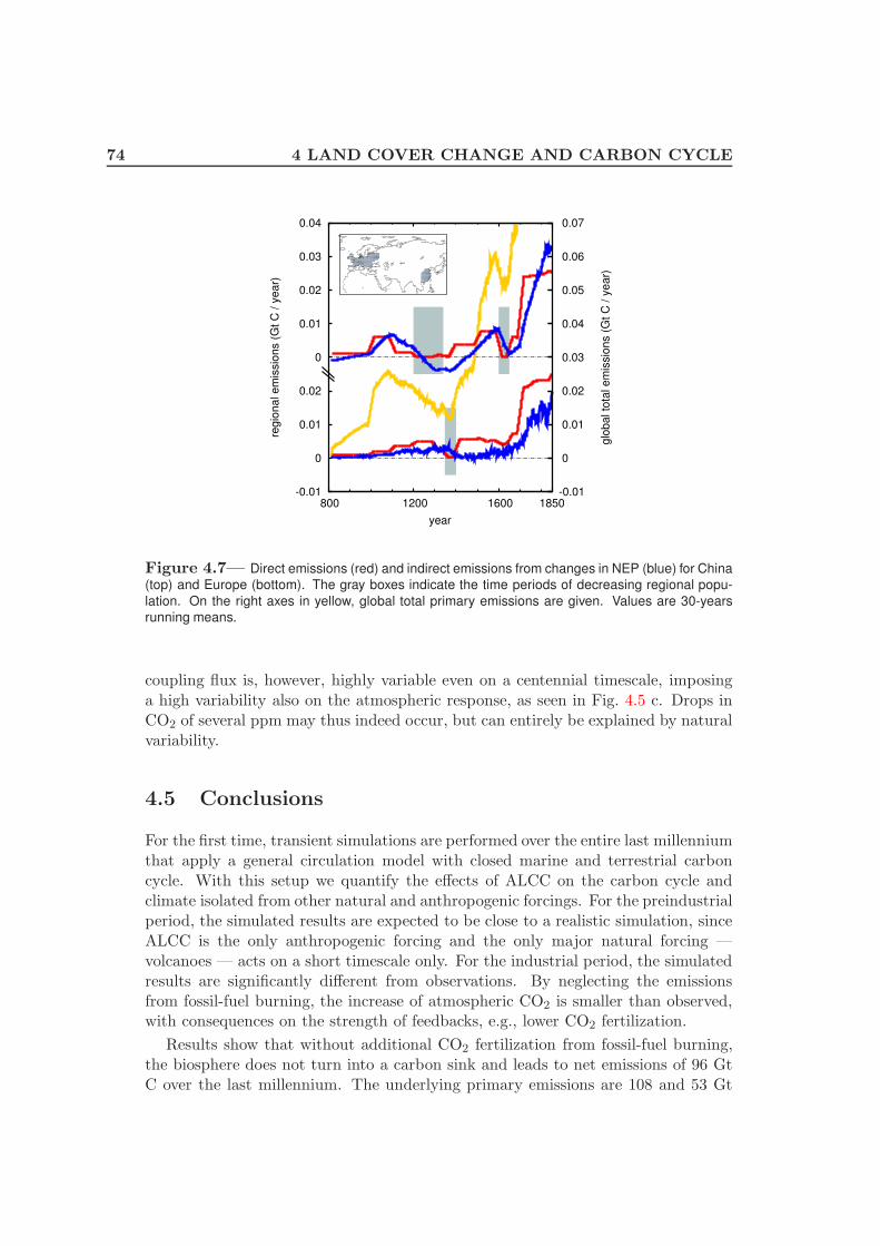
74 4 LAND COVER CHANGE AND CARBON CYCLE
-0.01
0
0.01
0.02
0
0.01
0.02
0.03
0.04
1850 800 1200 1600-0.01
0
0.01
0.02
0.03
0.04
0.05
0.06
0.07
reg
ion
al e
mis
sio
ns (
Gt
C /
ye
ar)
glo
ba
l to
tal e
mis
sio
ns (
Gt
C /
ye
ar)
year
Figure 4.7— Direct emissions (red) and indirect emissions from changes in NEP (blue) for China
(top) and Europe (bottom). The gray boxes indicate the time periods of decreasing regional popu-
lation. On the right axes in yellow, global total primary emissions are given. Values are 30-years
running means.
coupling flux is, however, highly variable even on a centennial timescale, imposinga high variability also on the atmospheric response, as seen in Fig. 4.5 c. Drops inCO2 of several ppm may thus indeed occur, but can entirely be explained by naturalvariability.
4.5 Conclusions
For the first time, transient simulations are performed over the entire last millenniumthat apply a general circulation model with closed marine and terrestrial carboncycle. With this setup we quantify the effects of ALCC on the carbon cycle andclimate isolated from other natural and anthropogenic forcings. For the preindustrialperiod, the simulated results are expected to be close to a realistic simulation, sinceALCC is the only anthropogenic forcing and the only major natural forcing —volcanoes — acts on a short timescale only. For the industrial period, the simulatedresults are significantly different from observations. By neglecting the emissionsfrom fossil-fuel burning, the increase of atmospheric CO2 is smaller than observed,with consequences on the strength of feedbacks, e.g., lower CO2 fertilization.
Results show that without additional CO2 fertilization from fossil-fuel burning,the biosphere does not turn into a carbon sink and leads to net emissions of 96 GtC over the last millennium. The underlying primary emissions are 108 and 53 Gt
4.5 Conclusions 75
C for the industrial and preindustrial period, respectively. We have quantified thefeedback of CO2 emissions on land carbon uptake to be high especially during thepreindustrial era: Here, the biosphere-atmosphere coupling reduces the impact ofALCC by 48%. Together with ocean uptake, only 21% of the emissions remainairborne. This keeps the human impact on atmospheric CO2 small over much of thepreindustrial times, which is in agreement with estimates by Olofsson and Hickler[2008], Strassmann et al. [2008]. However, by late medieval times atmospheric CO2
rises above natural variability. Our study thus suggests that with respect to globalCO2 concentration, the “Anthropocene” began prior to the industrialization.
We also investigated the effects of rapid changes in ALCC as occurred in severalregions over the last millennium due to epidemics and warfare. Indirect emissionsfrom past ALCC can be overcome by carbon storage in regrowing vegetation onlyfor events of long-lasting impact on population numbers. Only then regional carbonuptake occurs. The concurrent agricultural expansion in other regions, however,renders these events ineffective on the global scale. Such events thus cannot be themajor cause for observed drops in global CO2, as had been suggested by previousstudies. It seems more likely that local climate has been altered due to the fastchanges in biogeophysical fluxes [Pongratz et al., 2009].
This study applies an estimate of maximum ALCC to give an upper limit ofpossible human impact with respect to uncertainties in reconstructing land cover.Primary emissions are higher in this case, but the net effect on CO2 and global meantemperature is little altered. The only forcing taken into account is the change inagricultural extent. Other types of ALCC such as deforestation for wood harvest arenot included, but, as explained, are unlikely to have a major impact on our results.The long timescale further reduces the influence of uncertain parameters such as thedecomposition rates of carbon released during ALCC. Largely unknown, however,are preindustrial land management practices in their impact on the carbon cycle.Low-tillage practices, for example, are known to reduce CO2 fluxes from soils [e.g.,Reicosky et al., 1997], but base data to follow changes in management techniquesglobally and through the last millennium does not exist. Since the largest emissionsarise from vegetation carbon and since restorage occurs mainly on natural areas, weexpect our results to be generally robust.
The present study is relevant beyond the historical perspective in several points.First, an analysis of sub-fluxes suggests that a large fraction of the land-use ampli-fier effect results from the indirect emissions and thus from past ALCC, rather thanfrom the change in current turnover rates. Our analysis does not suggest that thereis less importance of including this effect in estimates for future climate change, butit indicates that a second process acts next to the change in turnover rates. Beingindirect emissions, this second process may either be reported as part of the primary(“book-keeping”) emissions, or as part of the land-use amplifier effect, but must notbe double-counted. It further is highly dependent on the assumptions made con-cerning the decay time of soil carbon on a decadal timescale. Model comparison andsensitivity studies should in the future aim at quantifying both processes separatelywith the associated uncertainty ranges.
76 4 LAND COVER CHANGE AND CARBON CYCLE
Second, this study has found an anthropogenic influence on atmospheric CO2 bylate medieval times, and has indicated significant changes in the land and oceancarbon content even earlier. The carbon balance has already for this reason beenconsiderably out of equilibrium for many centuries. Furthermore, one third of theALCC emissions until today have already been released by the end of the preindus-trial era. This early disturbance of the carbon balance does not only imply a legacyof the past by increasing the potential for anthropogenic climate change alreadyprior to industrialization. It also implies that the beginning of the simulation periodusually applied for climate projections may be too late — our results indicate thatclimate-carbon cycle studies for present and future centuries, which usually startfrom an equilibrium state around 1850, start from a significantly disturbed state ofthe carbon cycle, possibly distorting model calibration against the industrial period.
Acknowledgements
We thank Elke Stehfest for her help in extending the agricultural maps into thefuture, and Victor Brovkin and Katharina Six for helpful discussions. The sim-ulations of this study were carried out as part of the “Community Simulationsof the Last Millennium” (http://www.mpimet.mpg.de/en/wissenschaft/working-groups/millennium.html); we would like to thank all participants. We gratefullyacknowledge Reiner Schnur for setting up and performing the simulations. Thesewere carried out at the German Climate Computing Center (DKRZ).
77
Chapter 5
Biogeophysical Contributions tothe Effects of AnthropogenicLand Cover Change
Abstract
The biogeophysical effects of historical anthropogenic land cover change (ALCC) arecompared consistently to the biogeochemical effects on climate. For this, several sim-ulations with a coupled atmosphere/ocean general circulation model are performedtransiently over the last millennium applying ALCC as the only forcing. Biogeo-physical effects are found to exert only a weak influence on global mean temperature(−0.03 K) due to offsetting regional and seasonal effects, and teleconnections. Re-gionally, they may cause significant temperature changes in the 20th century, but notduring the preindustrial era. The rise in CO2 from ALCC emissions (about 20 ppmAD 800 to present) is therefore the driving force of the simulated global warming of0.13–0.15 K. Biogeophysical effects do further not contribute to the global restorageof carbon in the biosphere. The biosphere therefore mitigates ALCC emissions onlyvia its response to increased CO2. The weak climate response to biogeophysicaleffects contrasts with high radiative forcing from surface albedo changes; if radiativeforcing is used as estimate for global mean temperature, temperature change wouldbe overestimated by a factor of 4–5. The dominance of the biogeochemical effectsof ALCC has consequences also for the potential of climate change mitigation: Ifhistorical ALCC were reversed, most regions, including the northern mid- to highlatitudes, would contribute a cooling signal. This study highlights the need for anintegrated assessment of the different pathways of biosphere-atmosphere interactionto determine past and future effects of ALCC.
78 5 BIOGEOPHYSICAL EFFECTS OF LAND COVER CHANGE
5.1 Introduction
Anthropogenic land cover change (ALCC) represents one of the few climate forcingsfor which it is still not known whether they impose a global net cooling or warmingeffect. The analysis of ALCC is complex because it affects biosphere-atmospherefluxes through a multitude of partially counteracting processes. These processesare generally grouped into biogeophysical and biogeochemical mechanisms. Biogeo-physical mechanisms describe the influence on climate by the modification of thephysical properties of the land surface such as albedo, roughness, and evapotranspi-ration. Modeling studies suggest that through these biogeophysical effects, ALCC atmid- and high latitudes induces a cooling [e.g., Bonan et al., 1992, Claussen et al.,2001, Bounoua et al., 2002]. This is explained by the increase of surface albedoassociated with deforestation, which is caused by the snow masking effect of forestas well as by the higher snow-free albedo of non-forest vegetation. The differenceis particularly large during the winter and spring season for areas with snow cover,where albedo may change from 0.2 for forest to 0.8 on an open field [Robinson andKukla, 1984]. With the strong hydrological cycle in the tropics, the reduction ofroughness, leaf area, and rooting depth by deforestation reduces the evapotranspira-tion stronger than in the extra-tropics. Changes in plant physiology may thereforedominate over the albedo effect in the tropics so that ALCC can even lead to alocal warming [e.g., Claussen et al., 2001, Bounoua et al., 2002, DeFries et al., 2002].The loss of evapotranspiration in the tropics may again have a cooling effect on theextra-tropics due to the reduced atmospheric content of water vapor acting as green-house gas [e.g., Ganopolski et al., 2001, Sitch et al., 2005]. On the global scale, theopposing biogeophysical effects of ALCC partially cancel each other, but regionalclimate is significantly influenced by ALCC and may even affect remote areas viateleconnections [e.g., Chase et al., 2000]. Past studies on the biogeophysical effectsof historical ALCC have either performed transient simulations with Earth systemmodels of intermediate complexity (EMICs) [Brovkin et al., 1999, Bertrand et al.,2002, Bauer et al., 2003, Matthews et al., 2003], or equilibrium simulations withgeneral circulation models (GCMs) [Chase et al., 2000, Betts, 2001, Zhao et al.,2001, Bounoua et al., 2002, Davin et al., 2007].
Probably the most important biogeochemical mechanism of ALCC is the influenceon the carbon cycle, and the associated impact on the global CO2 concentration.Altering atmospheric CO2, ALCC modifies the Earth’s energy balance and thusclimate. ALCC constitutes a source of emissions mainly from the loss of terres-trial biomass. About one third of the anthropogenic CO2 emissions over the last150 years are estimated to be the direct consequence of ALCC [Houghton, 2003].Counteracting the emissions is an increased carbon uptake by both natural and agri-cultural vegetation, the so-called “residual land sink” [Denman et al., 2007]. Uptakeof CO2 by the ocean constitutes another sink of ALCC emissions. Coupled simula-tions that isolated the effects of ALCC quantified an increase of atmospheric CO2 ofabout 20 ppm over the last millennium after ocean uptake and biospheric restorage(Brovkin et al. [2004], Chapter 4). While the biogeophysical effects of ALCC have
5.1 Introduction 79
a more regional impact on climate, the altered carbon fluxes are felt globally sinceatmospheric CO2 is well mixed.
The overall picture so far is that with respect to ALCC most studies agree on (1)a global mean cooling from biogeophysical effects with pronounced cooling in thehighly cultivated midlatitudes of Eurasia and counteracting biogeophysical effects inthe tropics, and (2) a global warming from an increased atmospheric CO2 concen-tration. Most studies have just addressed single aspects and do thus not allow forcomplete conclusions. Some studies, however, have contrasted biogeophysical andbiogeochemical effects for certain scenarios: Claussen et al. [2001] have performedsensitivity studies of complete deforestation and afforestation in zonal belts, findingthat tropical deforestation tends to warm the planet due to dominating biogeochem-ical mechanisms, while in mid and high northern latitudes biogeophysical processesof deforestation lead to a global cooling. Betts [2000], Bala et al. [2007] determinedthat there is no gain for climate protection if abandoned agricultural areas in thenorthern midlatitudes are reforested. Studies using EMICs have analyzed both indi-vidually and in combination biogeophysical and biogeochemical effects of historicalALCC: Matthews et al. [2004] for the last 150, and Brovkin et al. [2004] for the last1000 years. It needs to be noted that the latter study did not rely on reconstructedland cover prior to AD 1700, but linearly interpolates between a state of potentialvegetation in the year AD 1000 and AD 1700. Nevertheless, these two publicationsmay be the most complete studies for the actual influence of ALCC on climate:First, they address both mechanism groups consistently with the same data andmethod. Second, they have a long enough history, which is crucial for atmosphericCO2, since primary emissions may accumulate in the atmosphere over time. Thetwo studies agree in (1) an overall cooling caused by biogeophysical mechanisms anda warming caused by biogeochemical mechanisms and (2) a similar magnitude ofboth effects. However, their conclusions concerning the net effect of biogeophysicaland biogeochemical mechanisms are contradicting: While Brovkin et al. [2004] finda net cooling of −0.05 K over the last millennium, Matthews et al. [2004] suggesta net warming of about 0.14 K over the last 150 years. In the present study wetry to give an improved estimate of the strength of the two individual effects anddetermine the sign of the net effect. We go beyond the previous studies in twoimportant aspects: (1) We apply a detailed reconstruction of ALCC over the lastmillennium. The reconstruction includes ALCC due to cropland and pasture withsub-grid information and specific allocation rules for agriculture on the differenttypes of natural vegetation. (2) We couple our land surface scheme to a generalcirculation model (GCM) for the atmosphere and the ocean. This allows a compar-atively high spatial resolution, which is crucial to capture realistically the effects ofsuch a heterogeneous forcing as ALCC. Unlike the two EMIC studies, this modelfurther takes into account natural internal variability, which is important to makestatements concerning the significance of ALCC-induced climate changes in relationto internal climate variability.
80 5 BIOGEOPHYSICAL EFFECTS OF LAND COVER CHANGE
5.2 Model and data
The atmosphere/ocean general circulation model (AOGCM) consists of ECHAM5[Roeckner et al., 2003] at T31 (approximately 4 degree) resolution with 19 verticallevels representing the atmosphere, and MPI-OM [Marsland et al., 2003] at 3 de-gree resolution with 40 vertical levels representing the ocean. The two models arecoupled daily without flux correction. The closed carbon cycle is simulated in theocean biogeochemistry model HAMOCC5 [Wetzel et al., 2005] and the modularland surface scheme JSBACH [Raddatz et al., 2007]. HAMOCC5 simulates inor-ganic carbon chemistry as well as phyto- and zooplankton dynamics in dependenceof temperature, solar radiation, and nutrients. It also considers the buildup of de-tritus, its sinking, remineralization, and sedimentation. JSBACH distinguishes 12plant functional types (PFTs), including one crop type, which differ with respectto their phenology, morphological, and photosynthetic parameters. Their fractionalcoverage of each grid cell is prescribed from maps annually. For each PFT, thestorage of organic carbon on land occurs in five pools: living tissue, woody material,and a pool storing sugar and starches for the vegetation carbon, and two soil car-bon pools with a fast (about 1.5 years) and a slow turnover rate (about 150 years).ALCC alters the pool carbon contents by relocating vegetation carbon to the soiland soil carbon between the PFTs of decreasing and expanding area (Sec. 4.2.1).
For the present study, the model code is changed such that the biogeophysicaleffects of ALCC are isolated: Carbon pools do not experience a change in coverfractions, i.e. there is no ALCC-related relocation of carbon. Furthermore, ALCCconsequences on plant productivity are not allowed, i.e. gross primary productivity,autotrophic, and heterotrophic respiration are calculated as if the PFT distributionremained at the year AD 800. For this, canopy conductances for CO2 and for waterare treated differently: All variables depending on canopy conductance for CO2
are calculated using the land cover map of AD 800, while transpiration, dependingon canopy conductance for water, is calculated as usual on the prescribed ALCCmaps. The prescribed ALCC maps are also used as usual for the calculations ofmorphological and phenological variables such as albedo and roughness length.
As ALCC forcing, the reconstruction of global agricultural areas and land coverby Pongratz et al. [2008b] is applied. It contains fractional maps of 14 vegetationtypes at an annual timestep and a spatial resolution of 0.5 degree. The agriculturaltypes considered are cropland, C3 pasture, and C4 pasture. The reconstructionmerges published maps of agriculture from AD 1700 to 1992 and a population-basedapproach to quantify agriculture for each country for the time period AD 800 to1700. With this approach the general expansion of agriculture is captured as well asspecific historic events, such as epidemics and wars. An extension of the agriculturaland land cover maps into the future follows the A1B scenario [see Nakicenovic et al.,2000], superimposing changes in agricultural extent from the scenario maps on theALCC map of 1992, the last map available from the ALCC reconstruction.
Four simulations branch off from the equilibrium state of the year AD 800 that all
5.3 Climate response to ALCC 81
exclude any changes in greenhouse gases other than the interactively calculated CO2.They further exclude any changes in natural and anthropogenic forcings other thanALCC, i.e. changes in solar, orbital, volcanic forcings, and fossil-fuel-related CO2
emissions are not permitted. With this setup, it is thus possible to isolate the effectof ALCC on climate. Apart from a 1300-year-long control simulation (named ctrl),two transient simulations run until the year 2100 applying ALCC as the only forcing(LC): The first applies the middle-range (best-guess) ALCC reconstruction, the sec-ond applies the lower-range ALCC reconstruction (high land cover dynamics), withthe aims to give a best estimate and an upper limit of possible ALCC effects on thecarbon cycle and related climate change for the preindustrial period. These simula-tions assess the combined biogeochemical and biogeophysical effects of ALCC and allatmosphere-ocean-biosphere feedbacks. A third transient simulation (LCPh) appliesthe middle-range ALCC reconstruction to simulate exclusively the biogeophysicaleffects of ALCC including feedbacks. The difference LCCh = LC − LCPh approxi-mates the climate response to exclusively the biogeochemical effects of ALCC.
In addition to the coupled simulations described above, the carbon pools are re-calculated offline with the aim to separate the primary effect of ALCC on the carbonbalance prior to any feedbacks arising from the coupling with the climate and theatmospheric and marine part of the carbon cycle. In offline simulation L, the effectsof ALCC were re-calculated under the climate of the control simulation. L − ctrlthen isolates the primary CO2 emissions of ALCC prior to any feedbacks. L − LCand L − LCPh, on the other hand, isolates the carbon flux induced by coupling thebiosphere to the atmosphere (“coupling flux”) — under climate and CO2 altered byboth biogeophysical and biogeochemical effects and by biogeophysical effects only,respectively.
The following sections analyze the biogeophysical effects of ALCC as simulatedin our model and compare them to the full influence on climate and the carbon cyclefrom both biogeophysical and biogeochemical effects as described in Chapter 4. Theyfurther give a synopsis of these effects in view of the mitigation potential of ALCC,and revisit the radiative forcing concept introduced in Chapter 3. Some figures thatprovide additional detail on the biogeophysical effects that is less relevant in thecontext of this Chapter will be found in Appendix B.
5.3 Climate response to ALCC
The full or “net” effect of combined biogeophysical and biogeochemical mechanismsof ALCC is a global warming. It becomes significant during the last centuries sim-ulated in this study where ALCC is particularly strong (Fig. 5.1 a). This net effectincludes a small biogeophysical cooling, which, on the global mean, remains mostlywithin the limits of internal variability throughout history and future. When de-termining the biogeochemical response as difference between the net effect and thebiogeophysical response, it leads thus to a warming slightly higher than the neteffect. Averaged over the 20th century, a global and annual mean surface temper-

82 5 BIOGEOPHYSICAL EFFECTS OF LAND COVER CHANGE
-0.1
0
0.1
0.2
0.3
800 1000 1200 1400 1600 1800 2000
tem
pera
ture
(K
)
year
LCLCChLCPh
a) global
-0.4
-0.2
0
0.2
0.4
800 1000 1200 1400 1600 1800 2000
b) Europe
-0.2
0
0.2
800 1000 1200 1400 1600 1800 2000
year
c) Southeast Asia
Figure 5.1— (a) Changes in global mean annual surface temperature from ALCC. LCPh: bio-
geophysical effects. LCCh: biogeochemical effects. LC: net effect. Thick lines are best-guess ALCC,
thin lines are high land cover dynamic. The shaded area indicates the 5–95 percentile of the control
simulation for the net effect. (b–c) Biogeophysical effects for Europe (land area 0–50◦E,40–60◦N)
and Southeast Asia (land area 67–120◦E,10–40◦N). All values are 50-years running mean.
ature change of −0.03 K is found as response for the biogeophysical mechanisms, awarming of 0.15 and 0.13 K for the net effect (for best-guess ALCC and high landcover dynamics, respectively), and a consequent warming of 0.18 and 0.16 K for thebiogeochemical mechanisms (Tab. 5.1). While the entire land area is more stronglyaffected by the biogeochemical warming than the ocean, the biogeophysical coolingis particularly pronounced over the agricultural areas. The table further comparesour findings to the two previous studies that isolated the biogeophysical and biogeo-chemical responses. The net temperature rise found in the present study is close tothe estimate by Matthews et al. [2004], who also found a strongly dominating bio-geochemical response as the present study does. While our biogeochemical responseis close to the estimate by Brovkin et al. [2004] in absolute values, our biogeophysicalresponse is substantially smaller than both previous studies suggested. The next twosections will describe in more detail the two individual model responses and theirspatial patterns.
5.3.1 Biogeophysical mechanisms
The weak global and annual mean response to the biogeophysical mechanisms ofALCC of −0.03 K contrasts sharply with its regional importance. In Europe, NorthAmerica, China, and India annual mean temperature is decreased by 0.3–0.5 K, whilea warming is simulated for smaller regions in the tropics and subtropics (Fig. 5.2 a).The cooling in northern mid- and high latitudes is largely driven by an increase ofsurface albedo (Fig. 5.3, averages over agricultural land). A strong snow-maskingeffect is discernible in the seasonal analysis in App. B.1, leading to cooling of up to0.9 K in Northeast Europe in winter (compared to 1–2 K found e.g. by Betts [2001]).The albedo effect is dominating in the mid- and high latitudes on the annual mean
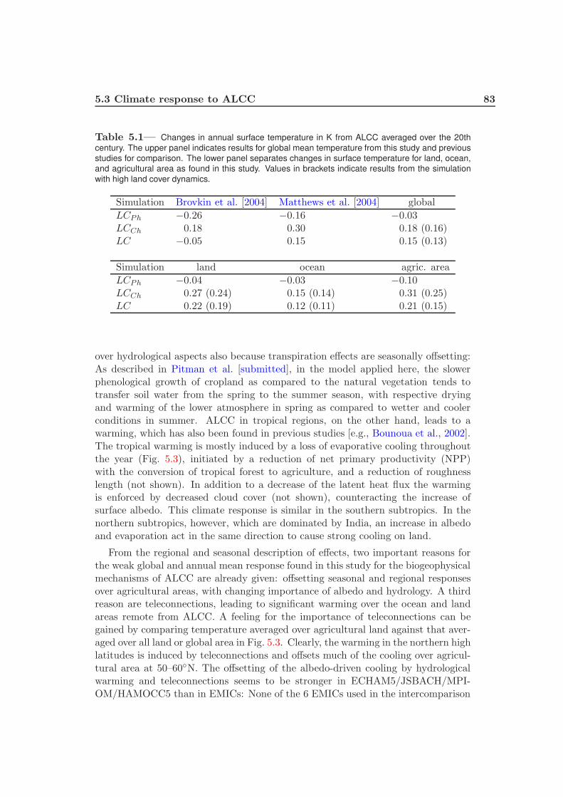
5.3 Climate response to ALCC 83
Table 5.1— Changes in annual surface temperature in K from ALCC averaged over the 20th
century. The upper panel indicates results for global mean temperature from this study and previous
studies for comparison. The lower panel separates changes in surface temperature for land, ocean,
and agricultural area as found in this study. Values in brackets indicate results from the simulation
with high land cover dynamics.
Simulation Brovkin et al. [2004] Matthews et al. [2004] global
LCPh −0.26 −0.16 −0.03LCCh 0.18 0.30 0.18 (0.16)LC −0.05 0.15 0.15 (0.13)
Simulation land ocean agric. area
LCPh −0.04 −0.03 −0.10LCCh 0.27 (0.24) 0.15 (0.14) 0.31 (0.25)LC 0.22 (0.19) 0.12 (0.11) 0.21 (0.15)
over hydrological aspects also because transpiration effects are seasonally offsetting:As described in Pitman et al. [submitted], in the model applied here, the slowerphenological growth of cropland as compared to the natural vegetation tends totransfer soil water from the spring to the summer season, with respective dryingand warming of the lower atmosphere in spring as compared to wetter and coolerconditions in summer. ALCC in tropical regions, on the other hand, leads to awarming, which has also been found in previous studies [e.g., Bounoua et al., 2002].The tropical warming is mostly induced by a loss of evaporative cooling throughoutthe year (Fig. 5.3), initiated by a reduction of net primary productivity (NPP)with the conversion of tropical forest to agriculture, and a reduction of roughnesslength (not shown). In addition to a decrease of the latent heat flux the warmingis enforced by decreased cloud cover (not shown), counteracting the increase ofsurface albedo. This climate response is similar in the southern subtropics. In thenorthern subtropics, however, which are dominated by India, an increase in albedoand evaporation act in the same direction to cause strong cooling on land.
From the regional and seasonal description of effects, two important reasons forthe weak global and annual mean response found in this study for the biogeophysicalmechanisms of ALCC are already given: offsetting seasonal and regional responsesover agricultural areas, with changing importance of albedo and hydrology. A thirdreason are teleconnections, leading to significant warming over the ocean and landareas remote from ALCC. A feeling for the importance of teleconnections can begained by comparing temperature averaged over agricultural land against that aver-aged over all land or global area in Fig. 5.3. Clearly, the warming in the northern highlatitudes is induced by teleconnections and offsets much of the cooling over agricul-tural area at 50–60◦N. The offsetting of the albedo-driven cooling by hydrologicalwarming and teleconnections seems to be stronger in ECHAM5/JSBACH/MPI-OM/HAMOCC5 than in EMICs: None of the 6 EMICs used in the intercomparison
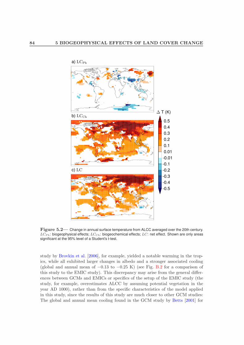
84 5 BIOGEOPHYSICAL EFFECTS OF LAND COVER CHANGE
-0.5
-0.4
-0.3
-0.2
-0.1
-0.01
0.01
0.1
0.2
0.3
0.4
0.5
∆ T (K)
a) LCPh
b) LCCh
c) LC
Figure 5.2— Change in annual surface temperature from ALCC averaged over the 20th century.
LCPh: biogeophysical effects; LCCh: biogeochemical effects; LC: net effect. Shown are only areas
significant at the 95% level of a Student’s t-test.
study by Brovkin et al. [2006], for example, yielded a notable warming in the trop-ics, while all exhibited larger changes in albedo and a stronger associated cooling(global and annual mean of −0.13 to −0.25 K) (see Fig. B.2 for a comparison ofthis study to the EMIC study). This discrepancy may arise from the general differ-ences between GCMs and EMICs or specifics of the setup of the EMIC study (thestudy, for example, overestimates ALCC by assuming potential vegetation in theyear AD 1000), rather than from the specific characteristics of the model appliedin this study, since the results of this study are much closer to other GCM studies:The global and annual mean cooling found in the GCM study by Betts [2001] for
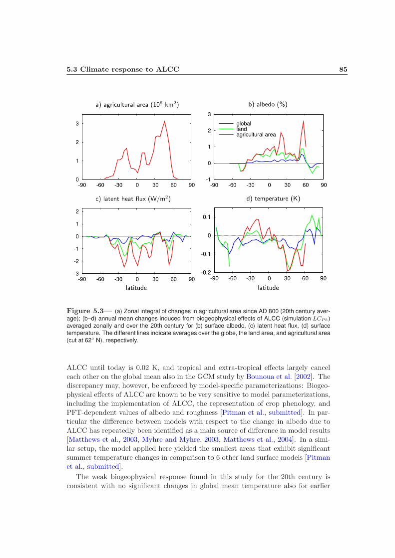
5.3 Climate response to ALCC 85
a) agricultural area (106 km2) b) albedo (%)
c) latent heat flux (W/m2) d) temperature (K)
latitude latitude
0
1
2
3
-90 -60 -30 0 30 60 90-1
0
1
2
3
-90 -60 -30 0 30 60 90
globallandagricultural area
-3
-2
-1
0
1
2
-90 -60 -30 0 30 60 90-0.2
-0.1
0
0.1
-90 -60 -30 0 30 60 90
Figure 5.3— (a) Zonal integral of changes in agricultural area since AD 800 (20th century aver-
age); (b–d) annual mean changes induced from biogeophysical effects of ALCC (simulation LCPh)
averaged zonally and over the 20th century for (b) surface albedo, (c) latent heat flux, (d) surface
temperature. The different lines indicate averages over the globe, the land area, and agricultural area
(cut at 62◦ N), respectively.
ALCC until today is 0.02 K, and tropical and extra-tropical effects largely canceleach other on the global mean also in the GCM study by Bounoua et al. [2002]. Thediscrepancy may, however, be enforced by model-specific parameterizations: Biogeo-physical effects of ALCC are known to be very sensitive to model parameterizations,including the implementation of ALCC, the representation of crop phenology, andPFT-dependent values of albedo and roughness [Pitman et al., submitted]. In par-ticular the difference between models with respect to the change in albedo due toALCC has repeatedly been identified as a main source of difference in model results[Matthews et al., 2003, Myhre and Myhre, 2003, Matthews et al., 2004]. In a simi-lar setup, the model applied here yielded the smallest areas that exhibit significantsummer temperature changes in comparison to 6 other land surface models [Pitmanet al., submitted].
The weak biogeophysical response found in this study for the 20th century isconsistent with no significant changes in global mean temperature also for earlier
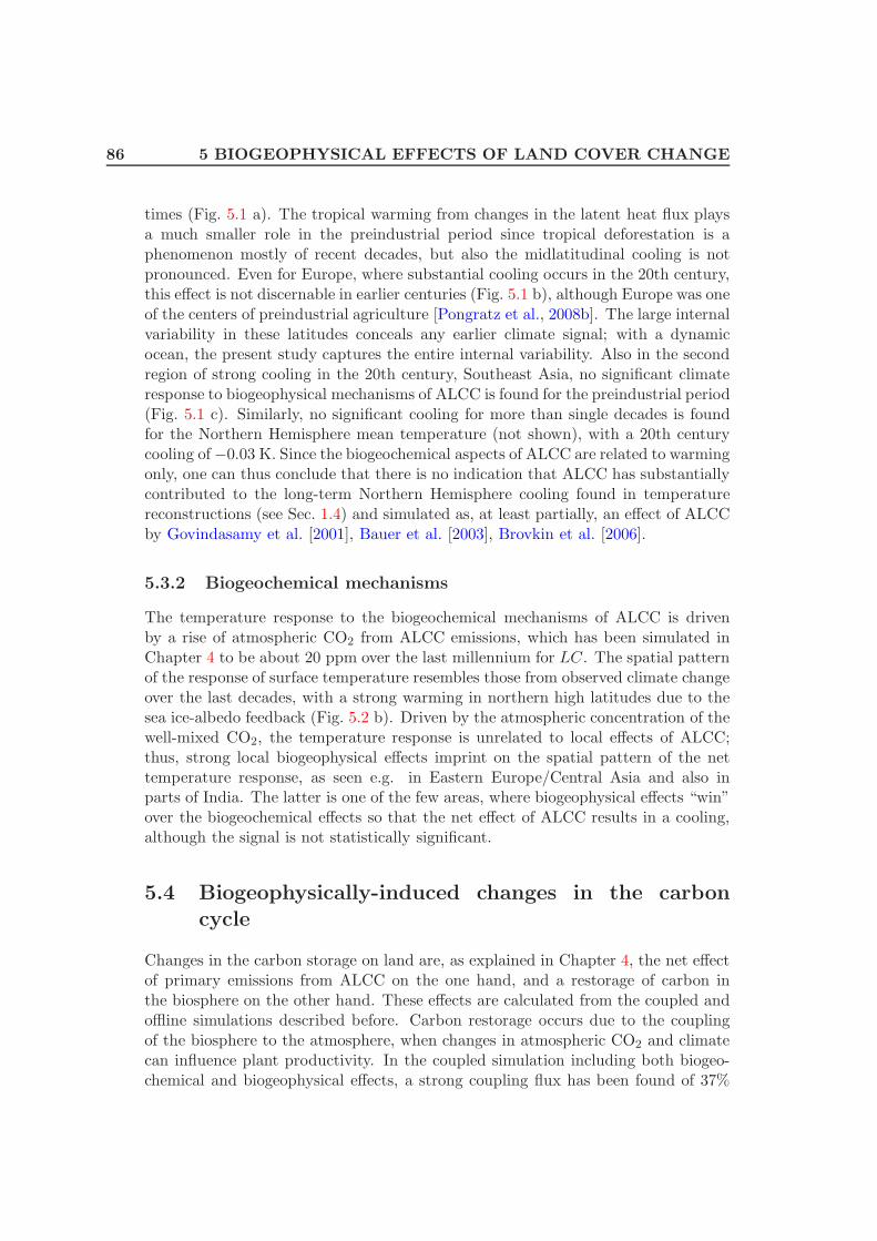
86 5 BIOGEOPHYSICAL EFFECTS OF LAND COVER CHANGE
times (Fig. 5.1 a). The tropical warming from changes in the latent heat flux playsa much smaller role in the preindustrial period since tropical deforestation is aphenomenon mostly of recent decades, but also the midlatitudinal cooling is notpronounced. Even for Europe, where substantial cooling occurs in the 20th century,this effect is not discernable in earlier centuries (Fig. 5.1 b), although Europe was oneof the centers of preindustrial agriculture [Pongratz et al., 2008b]. The large internalvariability in these latitudes conceals any earlier climate signal; with a dynamicocean, the present study captures the entire internal variability. Also in the secondregion of strong cooling in the 20th century, Southeast Asia, no significant climateresponse to biogeophysical mechanisms of ALCC is found for the preindustrial period(Fig. 5.1 c). Similarly, no significant cooling for more than single decades is foundfor the Northern Hemisphere mean temperature (not shown), with a 20th centurycooling of −0.03 K. Since the biogeochemical aspects of ALCC are related to warmingonly, one can thus conclude that there is no indication that ALCC has substantiallycontributed to the long-term Northern Hemisphere cooling found in temperaturereconstructions (see Sec. 1.4) and simulated as, at least partially, an effect of ALCCby Govindasamy et al. [2001], Bauer et al. [2003], Brovkin et al. [2006].
5.3.2 Biogeochemical mechanisms
The temperature response to the biogeochemical mechanisms of ALCC is drivenby a rise of atmospheric CO2 from ALCC emissions, which has been simulated inChapter 4 to be about 20 ppm over the last millennium for LC. The spatial patternof the response of surface temperature resembles those from observed climate changeover the last decades, with a strong warming in northern high latitudes due to thesea ice-albedo feedback (Fig. 5.2 b). Driven by the atmospheric concentration of thewell-mixed CO2, the temperature response is unrelated to local effects of ALCC;thus, strong local biogeophysical effects imprint on the spatial pattern of the nettemperature response, as seen e.g. in Eastern Europe/Central Asia and also inparts of India. The latter is one of the few areas, where biogeophysical effects “win”over the biogeochemical effects so that the net effect of ALCC results in a cooling,although the signal is not statistically significant.
5.4 Biogeophysically-induced changes in the carboncycle
Changes in the carbon storage on land are, as explained in Chapter 4, the net effectof primary emissions from ALCC on the one hand, and a restorage of carbon inthe biosphere on the other hand. These effects are calculated from the coupled andoffline simulations described before. Carbon restorage occurs due to the couplingof the biosphere to the atmosphere, when changes in atmospheric CO2 and climatecan influence plant productivity. In the coupled simulation including both biogeo-chemical and biogeophysical effects, a strong coupling flux has been found of 37%
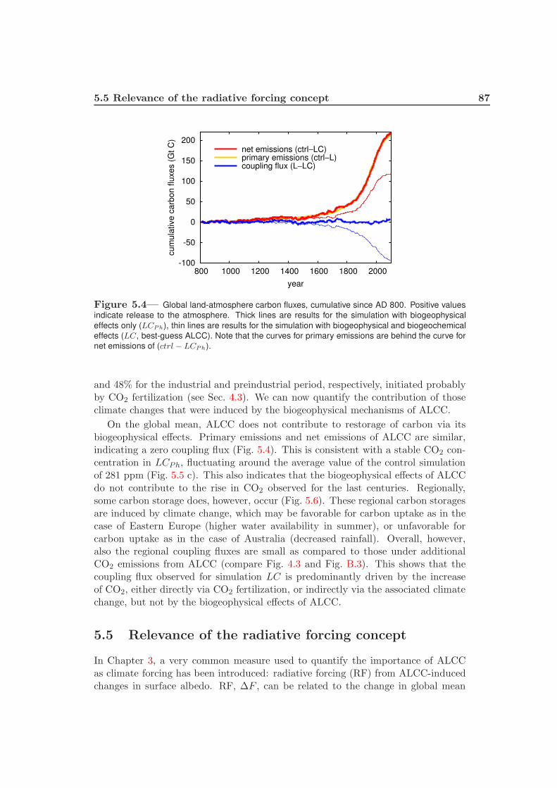
5.5 Relevance of the radiative forcing concept 87
-100
-50
0
50
100
150
200
800 1000 1200 1400 1600 1800 2000
cum
ula
tive c
arb
on f
luxes (
Gt
C)
year
net emissions (ctrl−LC)primary emissions (ctrl−L)coupling flux (L−LC)
Figure 5.4— Global land-atmosphere carbon fluxes, cumulative since AD 800. Positive values
indicate release to the atmosphere. Thick lines are results for the simulation with biogeophysical
effects only (LCPh), thin lines are results for the simulation with biogeophysical and biogeochemical
effects (LC, best-guess ALCC). Note that the curves for primary emissions are behind the curve for
net emissions of (ctrl − LCPh).
and 48% for the industrial and preindustrial period, respectively, initiated probablyby CO2 fertilization (see Sec. 4.3). We can now quantify the contribution of thoseclimate changes that were induced by the biogeophysical mechanisms of ALCC.
On the global mean, ALCC does not contribute to restorage of carbon via itsbiogeophysical effects. Primary emissions and net emissions of ALCC are similar,indicating a zero coupling flux (Fig. 5.4). This is consistent with a stable CO2 con-centration in LCPh, fluctuating around the average value of the control simulationof 281 ppm (Fig. 5.5 c). This also indicates that the biogeophysical effects of ALCCdo not contribute to the rise in CO2 observed for the last centuries. Regionally,some carbon storage does, however, occur (Fig. 5.6). These regional carbon storagesare induced by climate change, which may be favorable for carbon uptake as in thecase of Eastern Europe (higher water availability in summer), or unfavorable forcarbon uptake as in the case of Australia (decreased rainfall). Overall, however,also the regional coupling fluxes are small as compared to those under additionalCO2 emissions from ALCC (compare Fig. 4.3 and Fig. B.3). This shows that thecoupling flux observed for simulation LC is predominantly driven by the increaseof CO2, either directly via CO2 fertilization, or indirectly via the associated climatechange, but not by the biogeophysical effects of ALCC.
5.5 Relevance of the radiative forcing concept
In Chapter 3, a very common measure used to quantify the importance of ALCCas climate forcing has been introduced: radiative forcing (RF) from ALCC-inducedchanges in surface albedo. RF, ∆F , can be related to the change in global mean

88 5 BIOGEOPHYSICAL EFFECTS OF LAND COVER CHANGE
-220
-200
-180
-160
-140
-120
-100
-80
-60
-40
-20
0
20
800 1000 1200 1400 1600 1800 2000
carb
on invento
ry (
Gt C
)
year
LCLCPh5-95 percentile of control simulation
a) land
0
20
40
60
800 1000 1200 1400 1600 1800 2000
year
c) atmosphere
0
20
40
60
80
b) ocean+sediment
Figure 5.5— Change in the carbon stored globally on land, the ocean and sediment, and the at-
mosphere. Red lines are results for simulation LC including both biogeophysical and biogeochemical
effects of ALCC. Blue lines are results for simulation LCPh including only biogeophysical effects. Both
simulations apply the best-guess ALCC reconstruction. The yellow area indicates the 5–95 percentile
of the control simulation. Values are 10-years running means. This figure compares with Fig. 4.5;
note the different scale for (a) land.
surface temperature, ∆T , via the climate sensitivity parameter λ (see Sec. 1.5),
∆T = λ · ∆F . (5.1)
This RF is meant to represent the global mean climate response to biogeophysicaleffects of ALCC and is used as such e.g. in the reports by the IntergovernmentalPanel on Climate Change. In Chapter 4, the CO2 emissions from ALCC and theassociated increase in CO2 have been quantified. Though often subsumed as fossil-fuel-dominated anthropogenic emissions, this is the second important pathway ofdirect ALCC influence on temperature. The RF for ALCC-induced changes in CO2,∆FCO2
, can be estimated via the increase in atmospheric CO2, ∆C, in the two LCsimulations (best-guess ALCC and high land cover dynamics) after uptake by landand ocean, using the relationship [Myhre et al., 1998]
∆FCO2= 5.35 · ln(1 + ∆C/C0) . (5.2)
Here, C0 is the CO2 concentration at the beginning of the simulations.
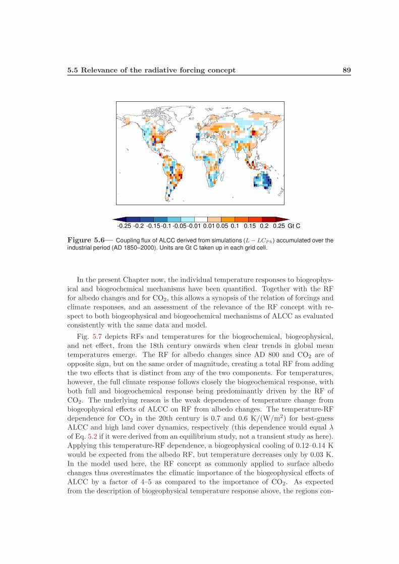
5.5 Relevance of the radiative forcing concept 89
-0.25 -0.2 -0.15-0.1 -0.05-0.01 0.01 0.05 0.1 0.15 0.2 0.25 Gt C
Figure 5.6— Coupling flux of ALCC derived from simulations (L − LCPh) accumulated over the
industrial period (AD 1850–2000). Units are Gt C taken up in each grid cell.
In the present Chapter now, the individual temperature responses to biogeophys-ical and biogeochemical mechanisms have been quantified. Together with the RFfor albedo changes and for CO2, this allows a synopsis of the relation of forcings andclimate responses, and an assessment of the relevance of the RF concept with re-spect to both biogeophysical and biogeochemical mechanisms of ALCC as evaluatedconsistently with the same data and model.
Fig. 5.7 depicts RFs and temperatures for the biogeochemical, biogeophysical,and net effect, from the 18th century onwards when clear trends in global meantemperatures emerge. The RF for albedo changes since AD 800 and CO2 are ofopposite sign, but on the same order of magnitude, creating a total RF from addingthe two effects that is distinct from any of the two components. For temperatures,however, the full climate response follows closely the biogeochemical response, withboth full and biogeochemical response being predominantly driven by the RF ofCO2. The underlying reason is the weak dependence of temperature change frombiogeophysical effects of ALCC on RF from albedo changes. The temperature-RFdependence for CO2 in the 20th century is 0.7 and 0.6 K/(W/m2) for best-guessALCC and high land cover dynamics, respectively (this dependence would equal λof Eq. 5.2 if it were derived from an equilibrium study, not a transient study as here).Applying this temperature-RF dependence, a biogeophysical cooling of 0.12–0.14 Kwould be expected from the albedo RF, but temperature decreases only by 0.03 K.In the model used here, the RF concept as commonly applied to surface albedochanges thus overestimates the climatic importance of the biogeophysical effects ofALCC by a factor of 4–5 as compared to the importance of CO2. As expectedfrom the description of biogeophysical temperature response above, the regions con-
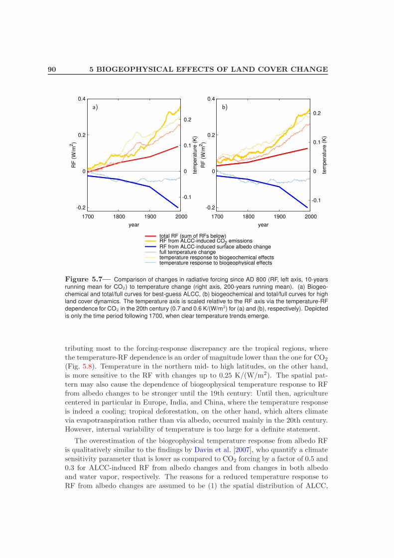
90 5 BIOGEOPHYSICAL EFFECTS OF LAND COVER CHANGE
-0.2
0
0.2
0.4
1700 1800 1900 2000
-0.1
0
0.1
0.2
RF
(W
/m2)
tem
pe
ratu
re (
K)
year
-0.2
0
0.2
0.4
1700 1800 1900 2000
-0.1
0
0.1
0.2
RF
(W
/m2)
tem
pe
ratu
re (
K)
year
total RF (sum of RFs below)RF from ALCC-induced CO2 emissionsRF from ALCC-induced surface albedo changefull temperature changetemperature response to biogeochemical effectstemperature response to biogeophysical effects
a) b)
Figure 5.7— Comparison of changes in radiative forcing since AD 800 (RF, left axis, 10-years
running mean for CO2) to temperature change (right axis, 200-years running mean). (a) Biogeo-
chemical and total/full curves for best-guess ALCC, (b) biogeochemical and total/full curves for high
land cover dynamics. The temperature axis is scaled relative to the RF axis via the temperature-RF
dependence for CO2 in the 20th century (0.7 and 0.6 K/(W/m2) for (a) and (b), respectively). Depicted
is only the time period following 1700, when clear temperature trends emerge.
tributing most to the forcing-response discrepancy are the tropical regions, wherethe temperature-RF dependence is an order of magnitude lower than the one for CO2
(Fig. 5.8). Temperature in the northern mid- to high latitudes, on the other hand,is more sensitive to the RF with changes up to 0.25 K/(W/m2). The spatial pat-tern may also cause the dependence of biogeophysical temperature response to RFfrom albedo changes to be stronger until the 19th century: Until then, agriculturecentered in particular in Europe, India, and China, where the temperature responseis indeed a cooling; tropical deforestation, on the other hand, which alters climatevia evapotranspiration rather than via albedo, occurred mainly in the 20th century.However, internal variability of temperature is too large for a definite statement.
The overestimation of the biogeophysical temperature response from albedo RFis qualitatively similar to the findings by Davin et al. [2007], who quantify a climatesensitivity parameter that is lower as compared to CO2 forcing by a factor of 0.5 and0.3 for ALCC-induced RF from albedo changes and from changes in both albedoand water vapor, respectively. The reasons for a reduced temperature response toRF from albedo changes are assumed to be (1) the spatial distribution of ALCC,
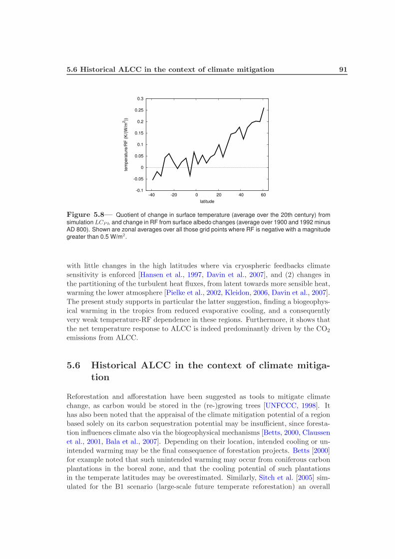
5.6 Historical ALCC in the context of climate mitigation 91
-0.1
-0.05
0
0.05
0.1
0.15
0.2
0.25
0.3
-40 -20 0 20 40 60
tem
pera
ture
/RF
(K
/(W
/m2))
latitude
Figure 5.8— Quotient of change in surface temperature (average over the 20th century) from
simulation LCPh and change in RF from surface albedo changes (average over 1900 and 1992 minus
AD 800). Shown are zonal averages over all those grid points where RF is negative with a magnitude
greater than 0.5 W/m2.
with little changes in the high latitudes where via cryospheric feedbacks climatesensitivity is enforced [Hansen et al., 1997, Davin et al., 2007], and (2) changes inthe partitioning of the turbulent heat fluxes, from latent towards more sensible heat,warming the lower atmosphere [Pielke et al., 2002, Kleidon, 2006, Davin et al., 2007].The present study supports in particular the latter suggestion, finding a biogeophys-ical warming in the tropics from reduced evaporative cooling, and a consequentlyvery weak temperature-RF dependence in these regions. Furthermore, it shows thatthe net temperature response to ALCC is indeed predominantly driven by the CO2
emissions from ALCC.
5.6 Historical ALCC in the context of climate mitiga-tion
Reforestation and afforestation have been suggested as tools to mitigate climatechange, as carbon would be stored in the (re-)growing trees [UNFCCC, 1998]. Ithas also been noted that the appraisal of the climate mitigation potential of a regionbased solely on its carbon sequestration potential may be insufficient, since foresta-tion influences climate also via the biogeophysical mechanisms [Betts, 2000, Claussenet al., 2001, Bala et al., 2007]. Depending on their location, intended cooling or un-intended warming may be the final consequence of forestation projects. Betts [2000]for example noted that such unintended warming may occur from coniferous carbonplantations in the boreal zone, and that the cooling potential of such plantationsin the temperate latitudes may be overestimated. Similarly, Sitch et al. [2005] sim-ulated for the B1 scenario (large-scale future temperate reforestation) an overall
92 5 BIOGEOPHYSICAL EFFECTS OF LAND COVER CHANGE
warming similar to the A2 scenario (large-scale tropical deforestation) due to strongbiogeophysical warming. All mentioned studies except for Betts [2000] performedcoupled simulations, which is problematic in the mitigation context since CO2 emis-sions mix in the atmosphere to give a local temperature signal that is not causedby local, but by global CO2 emissions. All mentioned studies except for Sitch et al.[2005] further performed idealized experiments only in which extreme scenarios ofcomplete deforestation and forestation over certain latitudinal bands were assumed.This theoretical consideration of the overall impact of maximum forestation on cli-mate can be contrasted to the question of the actual overall impact of ALCC untilpresent. For this purpose, the contribution of ALCC at each grid point to globalclimate change is estimated as described in the following 5 paragraphs.
First, the contribution of ALCC at each grid point to global climate change viathe biogeophysical mechanisms is assessed. For this, the change of RF from albedochanges between the years AD 800 and 1992 from Chapter 3 is used (Fig. 5.9 a).Though, as described in Sec. 5.5, RF from albedo changes may not be a good approx-imation of the overall climate response to biogeophysical effects, it is advantageousto use it here: As long as it is not clear whether the model applied in this studyhas a too weak biogeophysical climate response or the other models a too strongone (Sec. 5.3.1), it is more objective to rely on a measure that is similar acrossmodels, which RF from albedo changes is (see Chapter 3). By using this measureas representation of the biogeophysical effects, a conservative, upper estimate of thebiogeophysical effects possibly counteracting RF from CO2 is given.
Second, the contribution of ALCC at each grid point via the biogeochemicalmechanisms is assessed. The method is as follows: Using Eq. 5.2, the primaryemissions from AD 800 until 1992 determined from the simulations L − ctrl (best-guess ALCC) can be translated into the RF from CO2 emissions for each grid point.The grid-point based usage of Eq. 5.2, however, introduces an error: Instead ofcalculating the RF of the global CO2 increase of 20 ppm, the RF is calculated foreach grid point individually and summed to give the global RF. This introduces anerror because RF does not depend linearly on CO2. An error estimate (App. C)shows, however, that the error is below 4% and can therefore be neglected in thisanalysis.
Primary emissions are scaled down to yield the RF as determined from the in-crease in atmospheric CO2 in Sec. 5.5 on the global mean. This is the same assubtracting proportionally to the primary emissions of each grid point the globalocean uptake over history as simulated in LC (best-guess ALCC), and the carbonrestorage on land due to the coupling effect as derived from L − LC. The readershould note that the described method of subtracting terrestrial carbon uptake fromprimary emissions does not duplicate the method of Sec. 4.3, where the coupling fluxhas already been subtracted from primary emissions, but in a spatially explicit formalso for the coupling flux, to yield a map of net emissions. The underlying reasonwhy the map of net emissions cannot be used here is that we need to clearly distin-guish between effects of ALCC that can be attributed to ALCC in a specific locationand those that cannot. Attributable effects are changes in carbon storage that are
5.6 Historical ALCC in the context of climate mitigation 93
caused directly by the local ALCC, and include primary emissions that depend onthe strength and type of ALCC a grid point is undergoing and the carbon therebylost at this grid point. Effects not attributable to ALCC of a specific location includethe coupling flux, which is initiated by primary emissions only via the pathway ofatmospheric CO2; atmospheric CO2, however, is globally well mixed and integratesover the emissions of all grid points, its effects on carbon uptake are therefore de-tached from the local source of CO2. Therefore, the terrestrial carbon uptake due tothe coupling effect needs to be globally summed and subtracted proportionally to thelocal primary emissions, independent of where it actually occurs. This principle alsoapplies to ocean uptake (here, it is obvious that the (ocean) map of carbon uptakecannot sensibly be subtracted from the (land) map of carbon emissions). Since bothocean and terrestrial carbon uptake are carbon sinks that are initiated by ALCC,they need to be taken into account as counteracting the primary emissions in orderto quantify the net effect of ALCC on CO2.
Overall, the estimate derived here for RF from ALCC-induced increase in atmo-spheric CO2 reflects the historical effect of ALCC including the transient history ofcarbon source and sink terms. This more closely simulates the true temporal evolu-tion of ALCC-induced changes in carbon fluxes than previous equilibrium studies.With this method, the individual contribution of each grid point to the global RFfrom CO2 is determined and shown in Fig. 5.9 b.
The map of RF from CO2 emissions until present is added to the map of RFfrom present albedo changes to yield the total RF shown in Fig. 5.9 c. Note that thecontent of this map is quite different from Fig. 5.2 c, which showed the temperaturechange from the coupled simulation: The present approach allows to assess thecontribution of ALCC in an individual grid cell to global climate change. Fig. 5.2 c,on the contrary, shows the net temperature change caused by the biogeochemicaland biogeophysical effects of ALCC, but not as intended in this section as beingattributable to ALCC of a specific location — the biogeophysical effects (Fig. 5.2 a)clearly include teleconnections that are caused by remote, not localized ALCC, andthe biogeochemical effects (Fig. 5.2 b) mainly capture the climate response to theglobally well-mixed CO2.
In Fig. 5.9 c, global mean RF is 0.35 W/m2 for CO2, −0.20 W/m2 for albedo, and0.15 W/m2 total RF (compare Fig. 5.7). Most regions exhibit a positive total RF,indicating that there, the increase of atmospheric CO2 by historical ALCC in a gridpoint has had a larger radiative effect than the increase in surface albedo resultingfrom the same ALCC. These regions include Europe, India, China, and regions withtropical forest. Some regions exhibit a negative total forcing due to either of tworeasons: (1) the increase in albedo induces a larger forcing than CO2 emissions, ason the U.S. West Coast, in Central Asia, the Eastern Amazon, and West Africa; or(2) the increase in albedo and changes in carbon stocks act in the same direction,since ALCC leads to carbon sequestration, as in Australia, South and East Africa,the Pampas, and Mexico. Only in these few regions of negative total forcing maylocal ALCC have had a mitigating effect on global warming in the past.

94 5 BIOGEOPHYSICAL EFFECTS OF LAND COVER CHANGE
-10
-8
-6
-4
-2
-0.1
0.1
2
4
6
8
10
∆ F (W/m2)
a) albedo RF
b) CO2 RF
c) total RF
Figure 5.9— Comparison of radiative forcing (RF), ∆F : (a) RF from ALCC-induced surface
albedo changes AD 800–1992, data as described in Chapter 3; (b) RF from ALCC-induced CO2
emissions AD 800–1992; (c) total RF as sum of (a) and (b).
What does this conversely mean for future mitigation potential? Reversing ALCCof the last millennium would, on a timescale long enough to let the ocean outgas whatit had taken up of ALCC emissions, simply reverse the total RF of Fig. 5.9 c. Thismeans that most regions would have a cooling potential when reversing them to theirvegetation cover of AD 800. In the transient history, however, this may not be themost plausible scenario: On a short timescale and with small changes in atmosphericCO2 ocean uptake would continue at an unchanged rate (approximately 0.2 Gt Cper year over the last 50 years of our simulation). Via the time lag in ocean responsepast ALCC would thereby add on the carbon sequestration potential of reversingALCC. Depending on how long ocean uptake continues, the total RF would become
5.7 Summary and conclusions 95
more negative and might even render those regions effective for climate mitigationwhere past ALCC led to cooling.
It may be appropriate that previous studies have warned that the climate changemitigation potential may be overestimated when we assume future scenarios inwhich, after replacing boreal coniferous forest with crops, agricultural area is againreforested (although currently, only 7% of agricultural expansion or 23% of deforesta-tion affects evergreen coniferous forest, Sec. 2.4). However, the mitigation potentialseems to be less overestimated when we look at the effects of past ALCC, the rever-sion of which is possibly the more realistic scenario as first step for future mitigation.The ALCC over the past has only in few regions lead to a cooling radiative effect.
5.7 Summary and conclusions
This study has isolated the climate response to the biogeophysical effects of ALCCfrom that to the biogeochemical effects. Both responses were simulated in the samecoupled atmosphere/ocean GCM, which allows to compare the responses consis-tently without differences in ALCC implementation and model parameterization.Applying a GCM allows a higher spatial resolution than previous EMIC studies,which is more adequate for a forcing as heterogeneous as ALCC. The setup fur-ther allows to compare signals to natural internal variability. By running the modeltransiently over the last millennium, we could estimate the coupled response, in-cluding feedbacks, to the evolving strength of ALCC over the last millennium. Adisadvantage of this study certainly is the fact that biogeochemical effects are notsimulated independently, but are derived as residual of a fully-coupled simulationand one allowing only biogeophysical mechanisms. Therefore, the effect identified ascontribution from biogeochemical mechanisms may also include possible synergies.However, in an EMIC study determining independently biogeophysical, biogeochem-ical, and full model response, Claussen et al. [2001] found that synergies are muchsmaller than pure contributions, which is also supported by the studies by Brovkinet al. [2004], Matthews et al. [2004]. Hence, one of the three responses may also inour study be approximated as residual of the two others. Considering that the bio-geophysical response of the EMICs differs substantially from GCMs, this remains,however, an open question until more GCM studies have been performed.
This study has found a global temperature change due to biogeophysical effectsthat is small as compared to the temperature response under both biogeophysicaland biogeochemical consequences of ALCC, namely −0.03 K as opposed to 0.13–0.15 K. While in Europe and Southeast Asia some regions show significant cooling inthe 20th century, changes are nowhere significant, as compared to internal variability,during the preindustrial era. Warming from ALCC-induced CO2 emissions is thuslittle dampened by biogeophysical cooling and leads to a significant warming inthe industrial period. The Northern Hemisphere cooling simulated is substantiallysmaller than found in previous studies and unlikely to have driven the long-termcooling leading to the “Little Ice Age”. A similar conclusion has been drawn in

96 5 BIOGEOPHYSICAL EFFECTS OF LAND COVER CHANGE
Chapter 3 based on estimates of RF from albedo changes only, and is confirmedhere by the coupled model response.
The small biogeophysical cooling contradicts high estimates of RF from ALCC-induced albedo changes. This contradiction indicates that RF from albedo changesis not an appropriate measure for the global impact of ALCC on climate, for whichthe concept has been applied [Forster et al., 2007]. The present study thereby sup-ports previous studies [Pielke et al., 2002, Davin et al., 2007], which have pointedout the importance of biogeophysical effects other than albedo. The usage of the“climate efficacy” concept [Hansen et al., 2005] has been proposed as solution. Theclimate efficacy is defined as ratio between the climate sensitivity to a given forcingsuch as ALCC and the climate sensitivity to CO2 and can be introduced as cor-recting factor to the RF-temperature relationship. However, as shown above thetemperature/RF-quotient depends strongly on the location of ALCC; the climateefficacy must therefore be expected to change with time as the spatial distributionof ALCC changes. For ALCC, coupled climate simulations and comparison to otherforcings based on temperature change therefore seem the best tool to assess theclimatic importance.
In addition to biogeophysical effects, the present study has estimated the tem-perature response to ALCC emissions consistently with the same model and data.Both on the global mean and for most regions, the forcing from CO2 emissions isthe driving force behind ALCC-induced temperature change. The dominance of thebiogeochemical effects of ALCC also has consequences for the potential of climatechange mitigation: When returning to a state of natural vegetation, most regions,including the northern mid- to high latitudes, would contribute a cooling signal toclimate change mitigation.
The carbon storage is found to be not affected by ALCC via its biogeophysicalmechanisms on the global scale, and is little affected on the regional scale. Thisindicates that only by CO2 emissions, ALCC alters climate and atmospheric com-position in a way that causes a global feedback on the carbon cycle — this feed-back had been identified as substantially counteracting primary emissions by bio-spheric restorage in Ch. 4. The biogeophysical effects of ALCC on carbon fluxesare, however, dependent on the climate scenario: This study has shown that in a cli-mate altered only by ALCC, the biogeophysical effects induce weak regional carbonsources and sinks, which cancel each other on the global scale. This picture maychange under the currently observed climate state of rising CO2 and global warm-ing: While the albedo changes and their radiative effects are not directly dependingon atmospheric CO2 concentration and temperature, or may become even weakerwith less snow cover, the reduction of evapotranspiration and consequent warmingin the tropics due to ALCC may become stronger. Increasing temperature maytip the respiration-photosynthesis balance of tropical forest in the direction of netemissions [Clark, 2004], especially when associated by a reduction in precipitation[Rodenbeck et al., 2003]. Biogeophysical effects can then be expected to counteractthe biogeochemically-induced coupling flux simulated in this study for the tropicalforest. All these considerations, however, are subject to large uncertainties concern-
5.7 Summary and conclusions 97
ing the complex interplay of temperature and moisture effects on photosynthesis andheterotrophic respiration [Clark, 2004].
This study has given a synopsis of different pathways, via which ALCC influencesclimate, from several perspectives: the influence on climate, the impact on thecarbon cycle, and the forcing-response relationship. It has highlighted the need foran integrated assessment of all terrestrial feedbacks on climate across different scales.Although on the global mean, biogeochemically-induced warming seems to be thedominating effect of historical ALCC, biogeophysical effects are strongly offsettingthis signal on the regional scale. Often, the latter one is more relevant, e.g. whenliving conditions and agricultural productivity are concerned. High spatial detailshould therefore be an emphasis also in future studies. It is crucial to apply theintegrated approach to historical ALCC in order to understand the past evolutionof climate, but also to accurately predict the future evolution and the mitigationpotential of ALCC scenarios.
Acknowledgements
I thank Victor Brovkin for providing me with the data of the EMIC intercomparisonstudy.


99
Chapter 6
Summary and Conclusion
6.1 Summary of methods
This thesis has assessed the influence of anthropogenic land cover change (ALCC)on the carbon cycle and the climate of the last millennium, with a special focus onthe, so far little-studied, preindustrial period. The methodological steps taken bythe author in this study are summarized in the following.
As a first step and prerequisite to the following modeling study, the climateperturbation under investigation has been quantified: Agricultural extent and theresulting changes in natural vegetation have been reconstructed globally with apopulation-based approach, building on published maps for the last 300 years. Re-gional specifics such as changes in cultures were integrated as far they could reason-ably be derived from literature. Uncertainties associated with this approach havebeen quantified using both modern and historical records. The resulting datasetsare being tested and applied in several projects outside this study (e.g., NCAR:Paleoclimate Reconstructions, NASA GISS: Modeling Paleo-Climates, Universityof Oxford: Millennium European Climate, Stanford Graduate School of Business).This dataset has then been applied as only forcing to a comprehensive climate modelto assess several aspects of biosphere-climate interactions in isolated and combinedform: First, the ECHAM5/JSBACH-model has been modified to simulate radiativeforcing (RF) from surface albedo changes. Second, from coupled simulations usingECHAM5/JSBACH/MPI-OM/HAMOCC5 (the simulations were carried out withhelp of the Millennium Group), the coupled climate response has been analyzed, withspecial focus on the carbon cycle. To our knowledge, these are the first transientsimulations over a millennial timescale using a comprehensive climate model thatincludes the closed carbon cycle. Third, this same model setup was applied to isolatethe biogeophysical effects of ALCC (the simulations were carried out with help of theMillennium Group). For this, the biosphere-atmosphere coupling was modified inthe model code. Overall, this study relied on model results from 154 years simulatedat T63 resolution with ECHAM5/JSBACH and 5200 years at T31 resolution withECHAM5/JSBACH/MPI-OM/HAMOCC5 (excluding approximately 4000 years ofmodel spinup).
100 6 SUMMARY AND CONCLUSION
6.2 Main findings concerning the beginning of the An-
thropocene
As explained in Chapters 1, 3, 4, and 5, there is no consensus in the scientificcommunity on whether humankind influenced significantly the climate prior to thelarge-scale burning of fossil-fuels in the industrial era. This study has investigatedthis topic at unprecedented detail with respect to both input datasets and modelsetup. The main findings are:
1. Cropland and pastures have been quantified to have increased from 2.8 (1.3–5.1 ·106 km2)1 to 7.7 ·106 km2 between AD 800 and 1700, causing a deforesta-tion of 2.1 (1.2–2.6 ·106 km2)1 (Chapter 2).
2. Surface albedo change from ALCC imposed a radiative forcing on the preindus-trial energy balance that is, on the global scale, one to two orders of magnitudesmaller than both the concurrent natural forcings and its strength during theindustrial period. It is thus unlikely to be the major driver of climate varia-tions such as the long-term Northern Hemisphere cooling including the “LittleIce Age”. In this respect, the present study contradicts earlier studies likeBrovkin et al. [1999], Govindasamy et al. [2001], Bauer et al. [2003], Goosseet al. [2006] (Chapter 3).
3. On the regional scale, RF estimates suggest a human-induced climate change:In “hot spots” such as India, the energy balance was altered at the samestrength as present-day CO2 forcing (Chapter 3). However, the signal in thecoupled climate including other biogeophysical processes and feedbacks re-mains within natural internal variability over the preindustrial period even inthe hot-spot regions (Chapter 5).
4. This study gives a new, more comprehensive estimate of preindustrial primaryemissions: primary emissions are simulated to amount to 53–61 Gt carbon(C) AD 800–1850 (excluding an estimated 10 Gt C for the earlier millennia)— 33–36% of the ALCC emissions until present (161–169 Gt C) (Chapter 4).This compares to emissions from fossil-fuel combustion of 321 Gt C [Marlandet al., 2008].
5. A high restorage of carbon by the biosphere occurs over the preindustrialperiod due to the coupling to climate and CO2 (48% of the primary emissions),most likely due to CO2 fertilization. As a consequence, the airborne fractionof CO2 amounts to only 21% (Chapter 4).
6. The strong coupling flux keeps the human impact on atmospheric CO2 lowerthan would be expected from the amount of primary emissions alone. Never-theless, the atmospheric CO2 concentration is significantly altered by ALCC
1The uncertainties around the best-guess estimate are compiled from Sec. 2.4 and 2.5. Anyranges given in the following refer to the best-guess and upper estimate of deforestation.
6.3 Main findings beyond the historical aspect 101
prior to industrialization: an increase by 5–6 ppm is simulated for AD 800 to1850 (Chapter 4).
7. With a CO2 increase by 5–6 ppm in this study for AD 800 to 1850, of whichonly about half developed prior to 1700, our estimate of a human impact onatmospheric CO2 is lower than suggested by the “early anthropogenic hypoth-esis” — at least 9 ppm were suggested by [Ruddiman, 2007]. A major advan-tage of the present study, and reason for the lower estimate, is the interactivesimulation of oceanic carbon uptake and carbon restorage in the biosphere(Chapter 4).
8. Unlike previously suggested, historic events are unlikely to have imprinted onCO2 as reconstructed from ice core records. The reasons are (1) indirect emis-sions from past ALCC (inhibiting regional carbon sequestration for all eventsexcept for the long-lasting Mongol invasion) and (2) concurrent emissions fromother parts of the world. Both effects have not been taken into account in pre-vious studies. The internal variability of the model suggests that CO2 drops ofseveral ppm may well be explained by internal variability instead (Chapter 4).
9. Global mean temperature is likely to have not been significantly altered byALCC during the preindustrial period (Chapters 4 and 5).
10. The model study suggests that, historically, warming from biogeochemical ef-fects of ALCC was stronger than cooling from biogeophysical effects concerningglobal mean temperature (Chapter 5).
In summary, the present study suggests that the Anthropocene did indeed beginprior to industrialization as far as atmospheric CO2 is concerned. An anthropogenicclimate change with respect to global mean temperature, on the other hand, cannotbe identified. The smaller amount of preindustrial emissions and the long timescaleover which they were emitted leaves the overall climate impact much smaller thanduring the industrial period, despite a significant disturbance of subsystems (e.g.,terrestrial carbon stocks).
6.3 Main findings beyond the historical aspect
1. An analysis of sub-fluxes suggests that a large fraction of the land-use amplifiereffect results from the indirect emissions and thus from past ALCC, ratherthan from the change in current turnover rates. The change in turnover ratesis not to be considered less important in estimates of future climate change,but it is complimented by a second process. Being indirect emissions, thissecond process may either be reported as part of the primary (“book-keeping”)emissions, or as part of the land-use amplifier effect, but must not be double-counted (Chapter 4).
102 6 SUMMARY AND CONCLUSION
2. There exists a legacy of preindustrial ALCC to the industrial period: Thisstudy has found an anthropogenic influence on atmospheric CO2 by late me-dieval times, and has indicated significant changes in the land and ocean carboncontent even earlier. It has further quantified a small loss of the additionalsink capacity due to ALCC over the preindustrial period. Due to all these fac-tors, the potential for anthropogenic climate change has been increased alreadyprior to industrialization (Chapter 4).
3. As consequence of the previous point, the carbon balance has been considerablyout of equilibrium for many centuries prior to the Industrial Revolution. Thisimplies that the beginning of the simulation period usually applied for climateprojections may be too late: Most climate-carbon cycle studies for presentand future centuries initialize their model from an equilibrium state around1850. However, at that point the carbon cycle was already in a significantlydisturbed state, as the present results indicate. This discrepancy may distortmodel calibration against the industrial period (Chapter 4).
4. There further exists a legacy of any past ALCC beyond its instantaneous ac-tion: This study has shown how indirect emissions continue several decadesbeyond the end of ALCC due to the disequilibrium between NPP and het-erotrophic respiration. This counteracts carbon storage in regrowing vegeta-tion, which has been exemplarily shown for several historic events. It alsoimplies that any mitigation efforts building on reforestation will lead to a car-bon sink only with a certain time lag (Chapter 4).
5. This study has reassessed the radiative forcing (RF) concept. It supportsprevious studies in that RF from surface albedo changes gives an incompleteindication of the full biogeophysical climate response. Going beyond this, thepresent study estimates consistently with the same model and data additionallythe biogeochemical effects on climate, which are found to dominate both theclimate response driven by albedo changes and by all biogeophysical effects(Chapter 5).
6. This study has assessed the mitigation potential of forestation from the histori-cal perspective, by quantifying the local contribution to the global net radiativeforcing from albedo effects and CO2 emissions (Chapter 5). The reversion ofpast ALCC would in most regions, including the mid- to high latitudes, leadto a cooling radiative effect.
6.4 Next steps to be taken
Expanding inclusiveness. This study has assessed ALCC as limited to the trans-formation of natural vegetation to agricultural areas. Other aspects of ALCC to bepossibly included in similar modeling studies are wood harvest, the influence ofshifting cultivation, and the interdependence of humans and fire (usage of fire for
6.4 Next steps to be taken 103
hunting, fire suppression). As described before, these aspects are most likely ofsubordinate influence compared to the ALCC treated in this study. Further ALCCprocesses to be possibly included, beyond the biogeophysical effects on climate andbiosphere-atmosphere exchange of carbon via CO2, are methane (CH4) emissions,impacts on nitrogen and other nutrient cycles, dust and aerosol emissions from opensoils and fires, changes in the hydrological cycle caused by irrigation, and soil erosion,salinization, and desertification.
Many of these missing model processes may be accounted for within the nextyears. However, data availability for the historical period will be a severe obstacle.A strong interaction across the disciplines of archeology, reconstruction of humanactivity via proxies such as pollen or charcoal, history, ecology, and modeling isneeded. In particular the global scale poses a problem: Many of the mechanisms ofhuman interference cannot be isolated from global cycles, so that statements abouthuman influence on a specific region are impossible even if all regional data wereavailable.
Statistical analysis. More rigorous statistics should be applied to detect humaninfluence in regions and times where it is small in comparison to natural internal vari-ability. This is the case, e.g., for the regional effects of biogeophysical mechanismsduring the preindustrial period. This “signal-to-noise” problem may be amplifiedby the fact that the model applied in the present study tends to overestimate ratherthan underestimate internal variability, in particular due to a too strong represen-tation of El Nino/Southern Oscillation (ENSO) [Jungclaus et al., 2006]. Due tothe internal variability in the climate system and its non-linear evolution, the de-tectability of a human fingerprint may further be facilitated by ensemble studies,i.e. several experiments of the same forcing, but with slightly different initial con-ditions. Ensemble studies could be particularly useful for studies on the effect ofhistoric events such as warfare and epidemics. These events alter the anthropogenicforcing on a short timescale, so that the forcing’s effect is more easily concealed bynatural variability than the general trend of agricultural expansion on the millennialtimescale.
Validation of biogeophysical model response. A detailed evaluation of theECHAM5/JSBACH model should indicate how accurately the biogeophysical re-sponse to ALCC is simulated and attribute errors to individual processes. Themodel is currently participating in a model intercomparison study for biogeophysi-cal impacts of ALCC on regional and global climate (“Land-Use and Climate, IDen-tification of robust impacts”, LUCID). Early results of the intercomparison studyhighlight the largely different response of atmosphere-biosphere models to the sameperturbation [Pitman et al., submitted]. A validation against observational data,however, has yet to be performed. As stated above, a validation of historical climateeffects of a perturbation against observational data is not feasible, especially whenthese effects shall be quantified in an isolated form from other forcings, unrelated to
104 6 SUMMARY AND CONCLUSION
real climate. However, databases such as FLUXNET (www.fluxnet.ornl.gov) couldbe used indirectly: By validating the model response for two different land covermaps against measurement stations in close proximity and with comparable envi-ronmental conditions, the change in climate variables from one land cover type toanother, represented as temporal evolution in the model, can be assessed in thespatial domain via observations. We would also like to better understand whichprocesses lead to the different climate responses across models — if it is rather theresponse to changes in surface albedo or to changes in the hydrological cycle. Thetwo effects both act with different signs in individual regions and seasons and mayoften counteract each other. The model responses towards changes in albedo and hy-drological cycle can be separated in a similar setup as it has been used in Chapter 5to split up biogeophysical and biogeochemical mechanisms; stomatal conductancefor CO2 and for water were treated differently in this setup, with the first experienc-ing no ALCC, while the second did. Similarly, stomatal conductance for water couldalso be excluded from experiencing ALCC, so that only albedo changes are allowedto act on climate. This would not only reveal the relative importance of changes inalbedo and hydrology, but also whether radiative forcing from albedo changes wouldat least be a good measure for the climate response to albedo changes.
Comparison against observational data. This study has delivered an impor-tant step towards a more complete understanding of the driving forces behind climatechange: It has quantified and analyzed one of the two dominant anthropogenic forc-ings, ALCC. This has been done over a time period long enough (1) to allow theaccumulation of the forcing (in particular with respect to atmospheric CO2), and (2)to cover different strengths of the forcing and its variability. Therefore, the changingimportance of ALCC in comparison to the other natural and anthropogenic climateforcings can be assessed, most notably to solar variability, orbital forcing, volcaniceruptions, and changes in greenhouse gas concentration from fossil-fuel combustion.Once similar quantifications of these other forcings have been conducted, as isolatedand combined studies, all forcings can be consistently compared against each otherin their importance for long-term climate trends and short-term climate variability,both globally and regionally. Model results for the combination of all known forcingscan eventually be compared against reconstructed climate for the last millenniumto assess the comprehensiveness of our understanding of past and present climatechange.
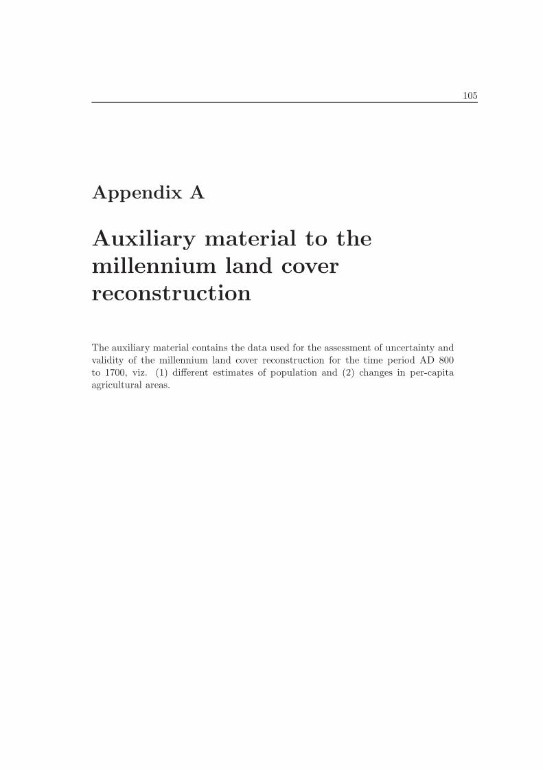
105
Appendix A
Auxiliary material to themillennium land coverreconstruction
The auxiliary material contains the data used for the assessment of uncertainty andvalidity of the millennium land cover reconstruction for the time period AD 800to 1700, viz. (1) different estimates of population and (2) changes in per-capitaagricultural areas.
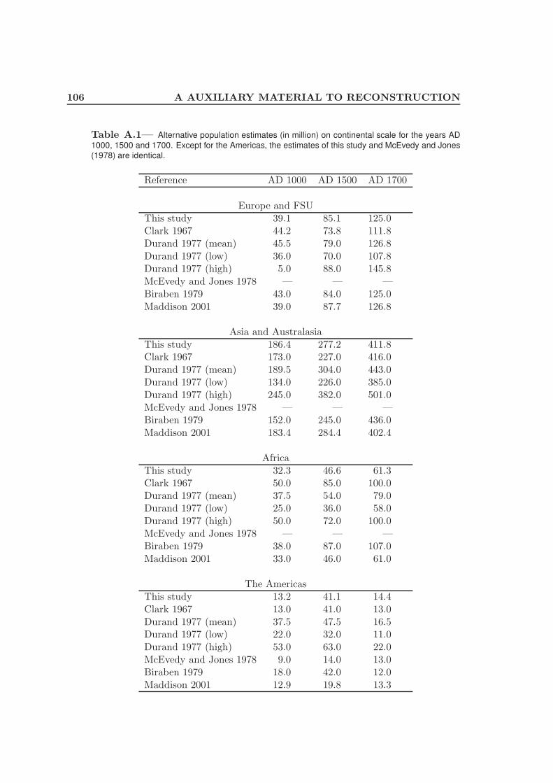
106 A AUXILIARY MATERIAL TO RECONSTRUCTION
Table A.1— Alternative population estimates (in million) on continental scale for the years AD
1000, 1500 and 1700. Except for the Americas, the estimates of this study and McEvedy and Jones
(1978) are identical.
Reference AD 1000 AD 1500 AD 1700
Europe and FSUThis study 39.1 85.1 125.0Clark 1967 44.2 73.8 111.8Durand 1977 (mean) 45.5 79.0 126.8Durand 1977 (low) 36.0 70.0 107.8Durand 1977 (high) 5.0 88.0 145.8McEvedy and Jones 1978 — — —Biraben 1979 43.0 84.0 125.0Maddison 2001 39.0 87.7 126.8
Asia and AustralasiaThis study 186.4 277.2 411.8Clark 1967 173.0 227.0 416.0Durand 1977 (mean) 189.5 304.0 443.0Durand 1977 (low) 134.0 226.0 385.0Durand 1977 (high) 245.0 382.0 501.0McEvedy and Jones 1978 — — —Biraben 1979 152.0 245.0 436.0Maddison 2001 183.4 284.4 402.4
AfricaThis study 32.3 46.6 61.3Clark 1967 50.0 85.0 100.0Durand 1977 (mean) 37.5 54.0 79.0Durand 1977 (low) 25.0 36.0 58.0Durand 1977 (high) 50.0 72.0 100.0McEvedy and Jones 1978 — — —Biraben 1979 38.0 87.0 107.0Maddison 2001 33.0 46.0 61.0
The AmericasThis study 13.2 41.1 14.4Clark 1967 13.0 41.0 13.0Durand 1977 (mean) 37.5 47.5 16.5Durand 1977 (low) 22.0 32.0 11.0Durand 1977 (high) 53.0 63.0 22.0McEvedy and Jones 1978 9.0 14.0 13.0Biraben 1979 18.0 42.0 12.0Maddison 2001 12.9 19.8 13.3
A AUXILIARY MATERIAL TO RECONSTRUCTION 107Table
A.2
—C
ha
ng
es
inp
er-
ca
pita
agri
cu
ltu
rala
rea
:nu
mb
ers
ind
ica
teh
igh
an
dlo
we
stim
ate
so
fch
an
ge
sin
cro
pa
nd
pa
stu
rea
rea
be
twe
en
AD
80
0a
nd
17
00
sh
ow
neve
ry1
00
ye
ars
an
dsca
led
to1
for
AD
17
00
.R
efe
ren
ce
sa
reg
ive
nin
the
ma
ind
ocu
me
nt.
Fo
rth
eA
me
rica
sa
nd
Au
str
ala
sia
,
valu
es
are
line
arl
yin
terp
ola
ted
toth
eo
ne
so
fth
ere
sp
ective
Old
Wo
rld
co
un
try
with
the
be
gin
nin
go
fE
uro
pe
an
se
ttle
me
nt.
Re
gio
nID
sin
the
firs
tlin
e:
1N
ort
hw
est
Eu
rop
e,
2N
ort
h,
Ce
ntr
ala
nd
Ea
st
Eu
rop
e,
3S
ou
thw
est
Me
dite
rra
ne
an
Eu
rop
e,
4E
aste
rnM
ed
ite
rra
ne
an
Eu
rop
ea
nd
So
uth
we
st
Asia
,5
Ch
ina
,Ta
iwa
n,
Ko
rea
,6
Ja
pa
n,
7O
the
rA
sia
,8
Me
dite
rra
ne
an
Afr
ica
,9
Ba
ntu
-in
flu
en
ce
dA
fric
a,
10
Oth
er
Afr
ica
,1
1N
ort
hA
me
rica
,1
2C
en
tra
la
nd
So
uth
Am
eri
ca
,1
3A
ustr
alia
an
dN
ew
Ze
ala
nd
.
Yea
r1
23
45
67
800
2.39
–1.
001.
43–
0.90
1.67
–0.
671.
33–
0.3
33.
65–
1.00
1.10
–0.
641.
50–
0.50
900
2.32
–1.
001.
36–
0.89
1.59
–0.
701.
30–
0.4
13.
33–
1.00
1.08
–0.
671.
44–
0.56
1000
2.23
–1.
001.
28–
0.86
1.52
–0.
741.
26–
0.4
83.
00–
1.00
1.05
–0.
701.
39–
0.61
1100
2.15
–1.
001.
20–
0.85
1.44
–0.
781.
22–
0.5
62.
68–
1.00
1.03
–0.
721.
33–
0.67
1200
1.94
–1.
001.
14–
0.84
1.37
–0.
811.
19–
0.6
32.
36–
1.00
1.00
–0.
751.
28–
0.72
1300
1.50
–1.
001.
08–
0.84
1.30
–0.
851.
15–
0.7
02.
04–
1.00
1.00
–0.
801.
22–
0.78
1400
1.37
–1.
001.
02–
0.85
1.22
–0.
891.
11–
0.7
81.
72–
1.00
1.00
–0.
841.
17–
0.83
1500
1.08
–1.
001.
00–
0.86
1.15
–0.
931.
07–
0.8
51.
35–
1.00
1.00
–0.
891.
11–
0.89
1600
1.00
–1.
001.
00–
0.85
1.07
–0.
961.
04–
0.9
31.
00–
0.98
1.00
–0.
941.
06–
0.94
1700
1.00
–1.
001.
00–
1.00
1.00
–1.
001.
00–
1.0
01.
00–
1.00
1.00
–1.
001.
00–
1.00
Yea
r8
910
1112
13
800
1.33
–0.
331.
00–
0.33
1.67
–0.
671.
50–
0.5
01.
67–
0.67
1.50
–0.
5090
01.
30–
0.41
1.00
–0.
411.
59–
0.70
1.44
–0
.56
1.59
–0.
701.
44–
0.56
1000
1.26
–0.
481.
00–
0.48
1.52
–0.
741.
39–
0.6
11.
52–
0.74
1.39
–0.
6111
001.
22–
0.56
1.00
–0.
561.
44–
0.78
1.33
–0
.67
1.44
–0.
781.
33–
0.67
1200
1.19
–0.
631.
00–
0.63
1.37
–0.
811.
28–
0.7
21.
37–
0.81
1.28
–0.
7213
001.
15–
0.70
1.00
–0.
701.
30–
0.85
1.22
–0
.78
1.30
–0.
851.
22–
0.78
1400
1.11
–0.
781.
00–
0.78
1.22
–0.
891.
17–
0.8
31.
22–
0.89
1.17
–0.
8315
001.
07–
0.85
1.00
–0.
851.
15–
0.93
1.11
–0
.89
1.15
–0.
931.
11–
0.89
1600
1.04
–0.
931.
00–
0.93
1.07
–0.
961.
06–
0.9
41.
07–
0.96
1.06
–0.
9417
001.
00–
1.00
1.00
–1.
001.
00–
1.00
1.00
–1.
001.
00–
1.00
1.00
–1.
00

109
Appendix B
Supplementary figures forbiogeophysical mechanisms
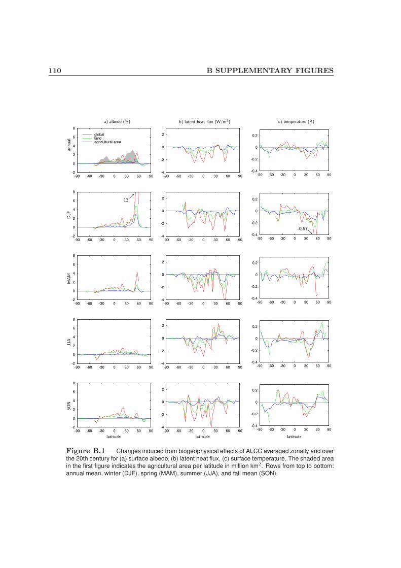
110 B SUPPLEMENTARY FIGURESan
nual
DJF
MAM
JJA
SO
N
a) albedo (%) b) latent heat flux (W/m2) c) temperature (K)
latitude latitude latitude
-2
0
2
4
6
8
-90 -60 -30 0 30 60 90
globallandagricultural area
-4
-2
0
2
-90 -60 -30 0 30 60 90
-0.4
-0.2
0
0.2
-90 -60 -30 0 30 60 90
-2
0
2
4
6
8
-90 -60 -30 0 30 60 90-4
-2
0
2
-90 -60 -30 0 30 60 90
-0.4
-0.2
0
0.2
-90 -60 -30 0 30 60 90
-2
0
2
4
6
8
-90 -60 -30 0 30 60 90-4
-2
0
2
-90 -60 -30 0 30 60 90
-0.4
-0.2
0
0.2
-90 -60 -30 0 30 60 90
-2
0
2
4
6
8
-90 -60 -30 0 30 60 90-4
-2
0
2
-90 -60 -30 0 30 60 90
-0.4
-0.2
0
0.2
-90 -60 -30 0 30 60 90
-2
0
2
4
6
8
-90 -60 -30 0 30 60 90-4
-2
0
2
-90 -60 -30 0 30 60 90
-0.4
-0.2
0
0.2
-90 -60 -30 0 30 60 90
13
-0.57
Figure B.1— Changes induced from biogeophysical effects of ALCC averaged zonally and over
the 20th century for (a) surface albedo, (b) latent heat flux, (c) surface temperature. The shaded area
in the first figure indicates the agricultural area per latitude in million km2. Rows from top to bottom:
annual mean, winter (DJF), spring (MAM), summer (JJA), and fall mean (SON).

B SUPPLEMENTARY FIGURES 111
-30
-25
-20
-15
-10
-5
0
-90 -60 -30 0 30 60 90
fore
st are
a (
% land a
rea)
latitude
-2
0
2
4
6
8
-90 -60 -30 0 30 60 90
alb
edo (
%)
latitude
CLIMBERECBILT-CLIO-VECODEKNMIMITMOBIDICUVICECHAM5/JSBACH
-0.08
-0.04
0
0.04
0.08
0.12
-90 -60 -30 0 30 60 90
eva
po
tra
nsp
ira
tio
n (
mm
/da
y)
latitude
-1.2
-0.8
-0.4
0
0.4
0.8
-90 -60 -30 0 30 60 90
su
rfa
ce
te
mp
era
ture
(K
)
latitude
Figure B.2— Comparison of simulation results with ECHAM5/JSBACH/MPI-OM/HAMOCC5
(ECHAM5/JSBACH in the following) to 6 Earth system models of intermediate complexity (EMICs).
Data for ECHAM5/JSBACH from simulations described in Chapter 5, data for EMICs from Brovkin
et al. [2006]. Shown are annual mean values averaged zonally over land or the globe as indicated.
The variables depicted are changes between the averaged 20th century and the control simulation
for AD 800 for ECHAM5/JSBACH, and changes between the final and initial 10-years average in
a simulation going from AD 1000 with an assumed state of potential natural vegetation to 1992 for
the EMICs. (a) Deforested area in percent of land area (note that if 1992, not 20th century aver-
age values were taken, ECHAM5/JSBACH would have slightly larger deforested area; note further
that EMICs assume potential vegetation for the beginning of their simulation in the year AD 1000,
while ECHAM5/JSBACH starts from a reconstructed land cover map in the year AD 800); (b) sur-
face albedo over land (note that for the EMICs, daily albedo values were averaged over the year
with the same weight, which emphasizes winter conditions. In Chapter 5 and for the orange line for
ECHAM5/JSBACH, albedo is calculated by dividing 100-year sums of reflected and incoming radia-
tion, which follows more closely the definition of climate-relevant albedo.); (c) evapotranspiration over
land (same as latent heat flux except for units); (d) global mean surface temperature.
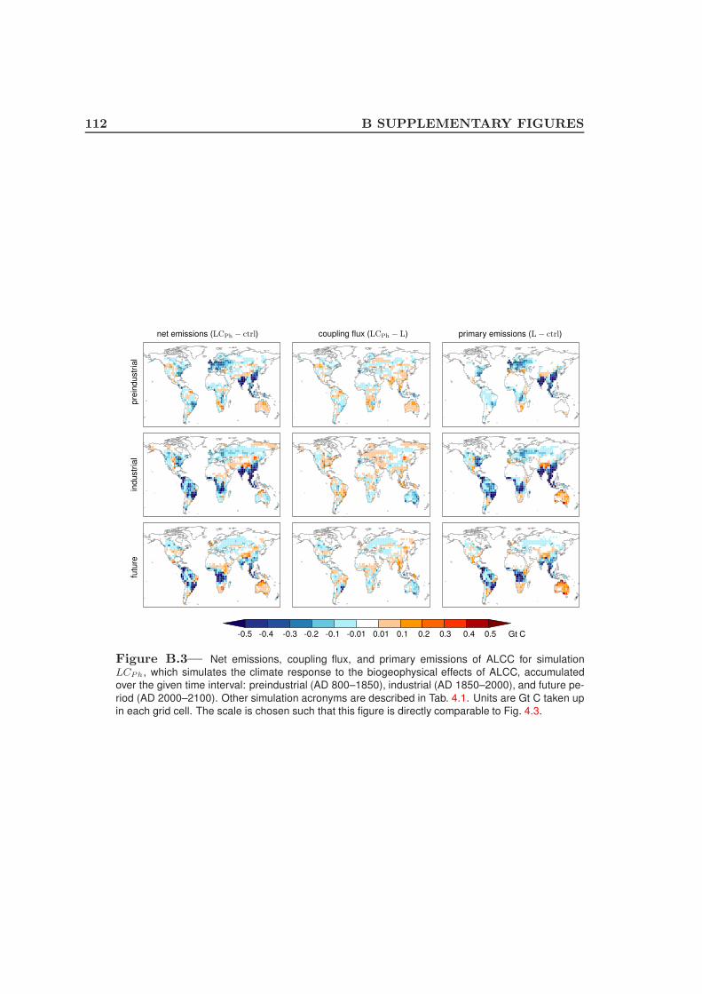
112 B SUPPLEMENTARY FIGURES
-0.5 -0.4 -0.3 -0.2 -0.1 -0.01 0.01 0.1 0.2 0.3 0.4 0.5 Gt C
primary emissions (L − ctrl)coupling flux (LCPh − L)net emissions (LCPh − ctrl)
futu
rein
dustr
ial
pre
industr
ial
Figure B.3— Net emissions, coupling flux, and primary emissions of ALCC for simulation
LCPh, which simulates the climate response to the biogeophysical effects of ALCC, accumulated
over the given time interval: preindustrial (AD 800–1850), industrial (AD 1850–2000), and future pe-
riod (AD 2000–2100). Other simulation acronyms are described in Tab. 4.1. Units are Gt C taken up
in each grid cell. The scale is chosen such that this figure is directly comparable to Fig. 4.3.
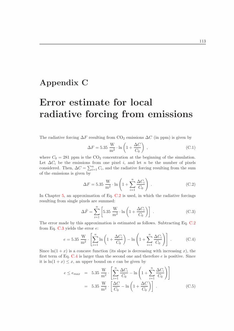
113
Appendix C
Error estimate for localradiative forcing from emissions
The radiative forcing ∆F resulting from CO2 emissions ∆C (in ppm) is given by
∆F = 5.35W
m2· ln
(
1 +∆C
C0
)
, (C.1)
where C0 = 281 ppm is the CO2 concentration at the beginning of the simulation.Let ∆Ci be the emissions from one pixel i, and let n be the number of pixelsconsidered. Then, ∆C =
∑ni=1
Ci, and the radiative forcing resulting from the sumof the emissions is given by
∆F = 5.35W
m2· ln
(
1 +
n∑
i=1
∆Ci
C0
)
. (C.2)
In Chapter 5, an approximation of Eq. C.2 is used, in which the radiative forcingsresulting from single pixels are summed:
∆F =
n∑
i=1
[
5.35W
m2· ln
(
1 +∆Ci
C0
)]
. (C.3)
The error made by this approximation is estimated as follows. Subtracting Eq. C.2from Eq. C.3 yields the error e:
e = 5.35W
m2·
[
n∑
i=1
ln
(
1 +∆Ci
C0
)
− ln
(
1 +n∑
i=1
∆Ci
C0
)]
. (C.4)
Since ln(1 + x) is a concave function (its slope is decreasing with increasing x), thefirst term of Eq. C.4 is larger than the second one and therefore e is positive. Sinceit is ln(1 + x) ≤ x, an upper bound on e can be given by
e ≤ emax = 5.35W
m2·
[
n∑
i=1
∆Ci
C0
− ln
(
1 +
n∑
i=1
∆Ci
C0
)]
= 5.35W
m2·
[
∆C
C0
− ln
(
1 +∆C
C0
)]
. (C.5)

114 C RADIATIVE FORCING ERROR ESTIMATE
0
0.1
0.2
0.3
0 20 40 60 80 100 0
5
10
15
20
em
ax (
W/m
2)
em
ax/∆
F (
%)
∆C (ppm)
emax
emax/∆F
Figure C.1— Maximum error in W/m2 (left axis) and in % (right axis) from the error estimate to
local radiative forcing from CO2 emissions.
Therefore, the error e is smaller than the error resulting from linearly approximatingln(1 + x) by the linear function x. Figure C.1 plots emax and the relative erroremax/∆F for values of ∆C = 0 . . . 100 ppm. The relative maximum error is 4% at∆C = 20 ppm and 17% at 100 ppm, the true error is consequently even smaller.
115
List of Figures
1.1 Map of anthropogenic land cover change until present . . . . . . . . 9
1.2 The world’s population . . . . . . . . . . . . . . . . . . . . . . . . . . 13
2.1 Scheme for reconstructing agricultural areas and land cover . . . . . 24
2.2 Maps of historical cropland . . . . . . . . . . . . . . . . . . . . . . . 36
2.3 Maps of historical pasture . . . . . . . . . . . . . . . . . . . . . . . . 37
2.4 Total area of crop and pasture for world regions AD 800–1992 . . . . 39
2.5 Total area of natural vegetation for world regions AD 800–1992 . . . 41
3.1 Global and hemispherical radiative forcing AD 800–1992 . . . . . . . 50
3.2 Maps for AD 800 and zonal means of radiative forcing AD 800–1992 51
3.3 Changes in radiative forcing during epidemics and warfare . . . . . . 53
4.1 Global land-atmosphere carbon fluxes AD 800–2100 . . . . . . . . . 62
4.2 Changes in vegetation and soil carbon pools and NEP AD 800–2100 64
4.3 Maps of net emissions, primary emissions, and coupling flux . . . . . 65
4.4 Disequilibria of soil respiration vs. NPP . . . . . . . . . . . . . . . . 67
4.5 Carbon inventory for land, ocean, and atmosphere AD 800–2100 . . 71
4.6 Change in global mean temperature AD 800–2100 . . . . . . . . . . 72
4.7 Carbon fluxes during epidemics and warfare . . . . . . . . . . . . . . 74
5.1 Temperature changes from different ALCC mechanisms AD 800–2100 82
5.2 Maps of temperature change for different ALCC mechanisms . . . . 84
5.3 Zonal plots of changes in albedo, latent heat flux, and temperature . 85
5.4 Global land-atmosphere carbon fluxes due to biogeophysical mechanism 87
5.5 Carbon inventory AD 800–2100 for biogeophysical simulation . . . . 88
5.6 Map of coupling flux due to biogeophysical mechanism . . . . . . . . 89
5.7 Comparison of radiative forcings to temperature responses . . . . . . 90
5.8 Zonal plot of temperature/radiative forcing . . . . . . . . . . . . . . 91
5.9 Maps of radiative forcing for albedo, CO2, and total forcing . . . . . 94
B.1 Seasonal zonal plots of changes in albedo, latent heat flux, and tem-perature . . . . . . . . . . . . . . . . . . . . . . . . . . . . . . . . . . 110

116 LIST OF FIGURES
B.2 Comparison with EMICs for biogeophysical effects . . . . . . . . . . 111
B.3 Maps of net emissions, coupling flux, and primary emissions for bio-geophysical simulation . . . . . . . . . . . . . . . . . . . . . . . . . . 112
C.1 Error estimate to local radiative forcing from emissions . . . . . . . . 114

117
List of Tables
2.1 Estimated global extent of land cover types AD 800–1992 . . . . . . 29
3.1 Comparison of (pre-)industrial radiative forcing across studies . . . . 50
4.1 Description of model simulations for carbon studies . . . . . . . . . . 61
4.2 Global atmosphere-biosphere carbon fluxes for different eras . . . . . 63
4.3 Primary emissions from anthropogenic land cover change . . . . . . 66
4.4 Carbon uptake by land, ocean, and atmosphere . . . . . . . . . . . . 70
5.1 Temperature changes in comparison to previous studies . . . . . . . 83
A.1 Alternative population estimates . . . . . . . . . . . . . . . . . . . . 106
A.2 Changes in per-capita agricultural area . . . . . . . . . . . . . . . . . 107

119
Bibliography
R.C. Allen. Economic structure and agricultural productivity in Europe, 1300–1800.European Review of Economic History, 3:1–25, 2000.
M. Andreae and P.J. Crutzen. Atmospheric aerosols: biogeochemical sources androle in atmospheric chemistry. Science, 276(5315):1052–1058, 1997.
M.O. Andreae and P. Merlet. Emission of trace gases and aerosols from biomassburning. Global Biogeochem. Cycles, 15(4):955–966, 2001.
D. Archer, H. Kheshgi, and E. Maier-Reimer. Multiple timescales for neutralizationof fossil fuel CO2. Geophys. Res. Lett., 24(4):405–408, 1997.
G.P. Asner, A.J. Elmore, L.P. Olander, R.E. Martin, and A.T. Harris. Grazingsystems, ecosystem responses, and global change. Ann. Rev. Environ. Resources,29:261–299, 2004.
G. Bala, K. Caldeira, M. Wickett, T.J. Phillips, D.B. Lobell, C. Delire, and A. Mirin.Combined climate and carbon-cycle effects of large-scale deforestation. PNAS, 104(16):6550–6555, 2007.
T. Barker, I. Bashmakov, A. Alharthi, M. Amann, L. Cifuentes, J. Drexhage,M. Duan, O. Edenhofer, B. Flannery, M. Grubb, M. Hoogwijk, F.I. Ibitoye, C.J.Jepma, W.A. Pizer, and K. Yamaji. Mitigation from a cross-sectoral perspective.In B. Metz, O.R. Davidson, P.R. Bosch, R. Dave, and L.A. Meyer, editors, Climate
Change 2007: Mitigation. Contribution of Working Group III to the Fourth As-
sessment Report of the Intergovernmental Panel on Climate Change, pages 619–690. Cambridge University Press, Cambridge, United Kingdom and New York,NY, USA, 2007.
E. Bauer and M. Claussen. Analyzing seasonal temperature trends in forcedclimate simulations of the past millennium. Geophys. Res. Lett., 33:L02702,doi:10.1029/2005GL024593, 2006.
E. Bauer, M. Claussen, and V. Brovkin. Assessing climate forcings of theEarth system for the past millennium. Geophys. Res. Lett., 30(6):1276,doi:10.1029/2002GL016639, 2003.

120 BIBLIOGRAPHY
F.A. Bazzaz. The response of natural ecosystems to the rising global CO2 levels.Annual Rev. Ecol. System., 21:167–196, 1990.
A. Berger. Milankovitch theory and climate. Rev. Geophys., 26:624–657, 1988.
C. Bertrand, M.F. Loutre, M. Crucifix, and A. Berger. Climate of the last millen-nium: a sensitivity study. Tellus, 54A:221–244, 2002.
R.A. Betts. Offset of the potential carbon sink from boreal forestation by decreasesin surface albedo. Nature, 408:187–190, 2000.
R.A. Betts. Biogeophysical impacts of land use on present-day climate: near-surface temperature change and radiative forcing. Atmos. Sci. Lett., 1:doi:10.1006/asle.2001.0023, 2001.
R.A. Betts, P.D. Falloon, K. Klein Goldewijk, and N. Ramankutty. Biogeophysicaleffects of land use on climate: Model simulations of radiative forcing and large-scale temperature change. Agric. For. Meteorol., 142:216–233, 2007.
J.N. Biraben. Essai sur l’evolution du nombre des hommes. Population, 34(1):13–25,1979.
B. Bolin, R. Sukumar, P. Ciais, W. Cramer, P. Jarvis, H. Kheshgi, C.A. Nobre,S. Semenov S, and W. Steffen. Global perspective. In R.T. Watson, I.R. No-ble, B. Bolin, N.H. Ravindranath, D.J. Verardo, and D.J. Dokken, editors, Land
Use, Land-Use Change, and Forestry - A Special Report of the IPCC. CambridgeUniversity Press, Cambridge, United Kingdom and New York, NY, USA, 2001.
G. Bonan. Ecological Climatology, chapter Land use and land-cover change, pages433–469. Cambridge University Press, Cambridge, 2002.
G.B. Bonan, D. Pollard, and S.L. Thompson. Effects of boreal forest vegetation onglobal climate. Nature, 359:716–718, 1992.
E. Boserup. The conditions of agricultural growth. Aldine, Chicago, 1965.
L. Bounoua, R.S. DeFries, G.J. Collatz, P.J. Sellers, and H. Khan. Effects of landcover conversion on surface climate. Climatic Change, 52:29–64, 2002.
V. Brovkin, A. Ganopolski, M. Claussen, C. Kubatzki, and V. Petoukhov. Modellingclimate response to historical land cover change. Glob. Ecol. and Biogeogr., 8:509–517, 1999.
V. Brovkin, S. Sitch, W. von Bloh, M. Claussen, E. Bauer, and W. Cramer. Role ofland cover changes for atmospheric CO2 increase and climate change during thelast 150 years. Global Change Biol., 10:1253–1266, 2004.
BIBLIOGRAPHY 121
V. Brovkin, M. Claussen, E. Driesschaert, T. Fichefet, D. Kicklighter, M.F. Loutre,H.D. Matthews, N. Ramankutty, M. Schaeffer, and A. Sokolov. Biogeophysicaleffects of historical land cover changes simulated by six Earth system models ofintermediate complexity. Clim. Dyn., 26:587–600, 2006.
V. Brovkin, T. Raddatz, C.H. Reick, M. Claussen, and V. Gayler. Global biogeo-physical interactions between forest and climate. Geophys. Res. Lett., submitted.
E.C. Brown de Colstoun, R.S DeFries, and J.R.G. Townshend. Evaluation of ISLSCPInitiative II satellite-based land cover data sets and assessment of progress in landcover data for global modeling. J. Geophys. Res., 111:D22S07, 2006.
T.N. Chase, R.A. Pielke Sr., T.G.F. Kittel, R.R. Nemani, and S.W. Running. Simu-lated impacts of historical land cover changes on global climate in northern winter.Clim. Dyn., 16:93–105, 2000.
C. Clark. Population growth and land use. Macmillan, London, 2nd edition, 1967.
D.A. Clark. Tropical forests and global warming: slowing it down or speeding it up?Front. Ecol. Environ., 2(2):73–80, 2004.
M. Claussen. Does land surface matter in climate and weather? In P. Kabat,M. Claussen, P.A. Dirmeyer, J.H.C. Gasha, L.B. de Guenni, M. Meybeck, R.A.Pielke Sr., C.J. Vorosmarty, R.W.A. Hutjes, and S. Lutkemeier, editors, Vegeta-
tion, Water, Humans and the Climate, pages 5–153. Springer, Berlin, 2004.
M. Claussen, V. Brovkin, and A. Ganopolski. Biogeophysical versus biogeochemicalfeedbacks of large-scale land cover change. Geophys. Res. Lett., 28(6):1011–1014,2001.
M. Claussen, V. Brovkin, R. Calov, A. Ganopolski, and C. Kubatzki. Did humankindprevent a Holocene glaciation? Climatic Change, 69:409–417, 2005.
Commission of the European Communities. Biofuels progress report: Report on the
progress made in the use of biofuels and other renewable fuels in the member states
of the European Union. COM(2006) 845 final, Brussels, 2006.
A.C. Crombie. Von Augustinus bis Galilei. Die Emanzipation der Naturwissenschaft.dtv, Wissenschaftliche Reihe, Munchen, 1977.
T.J. Crowley. Causes of climate change over the past 1000 years. Science, 289:270–277, 2000.
P.J. Crutzen and E.F. Stoermer. The “Anthropocene”. IGBP Newsletter, 41:17–18,2000.
E.L. Davin, N. de Noblet-Ducoudre, and P. Friedlingstein. Impact of land coverchange on surface climate: Relevance of the radiative forcing concept. Geophys.
Res. Lett., 34:L13702, 2007.

122 BIBLIOGRAPHY
R.S. DeFries, C.B. Field, I. Fung, G.J. Collatz, and L. Bounoua. Combining satellitedata and biogeochemical models to estimate global effects of human-induced landcover change on carbon emissions and primary productivity. Global Biogeochem.
Cycles, 13(3):803–815, 1999.
R.S. DeFries, L. Bounoua, and G.J. Collatz. Human modification of the landscapeand surface climate in the next fifty years. Global Change Biol., 8:438–458, 2002.
R.S. DeFries, J.A. Foley, and G.P. Asner. Land-use choices: balancing human needsand ecosystem function. Front. Ecol. Environ., 2(5):249–257, 2004.
K.L. Denman, G. Brasseur, A. Chidthaisong, P. Ciais, P.M. Cox, R.E. Dickinson,D. Hauglustaine, C. Heinze, E. Holland, D. Jacob, U. Lohmann, S. Ramachan-dran, P.L. da Silva Dias, S.C. Wofsy, and X. Zhang. Couplings Between Changesin the Climate System and Biogeochemistry. In S. Solomon, D. Qin, M. Manning,Z. Chen, M. Marquis, K.B. Averyt, M. Tignor, and H.L. Miller, editors, Climate
Change 2007: The Physical Science Basis. Contribution of Working Group I to
the Fourth Assessment Report of the Intergovernmental Panel on Climate Change.Cambridge University Press, Cambridge, United Kingdom and New York, NY,USA, 2007.
J. Diamond. Guns, Germs, and Steel. W. W. Norton & Company, New York,London, 1999.
I. Douglas. Human settlements. In W.B. Meyer and B.L. Turner II, editors, Changes
in Land Use and Land Cover: A Global Perspective, pages 149–170. CambridgeUniversity Press, Cambridge, 1994.
J.D. Durand. Historical estimates of world population: An evaluation. Popul.
Develop. Rev., 3(3):253–296, 1977.
J. Feddema, K. Oleson, G. Bonan, L. Mearns, W. Washington, G. Meehl, and D. Ny-chka. A comparison of a GCM response to historical anthropogenic land coverchange and model sensitivity to uncertainty in present-day land cover representa-tions. Clim. Dyn., 25:581–609, 2005.
F. Fehsenfeld, J. Calvert, R. Fall, P. Goldan, A.B. Guenther, C.N. Hewitt, B. Lamb,S. Liu, M. Trainer, H. Westberg, and P. Zimmermann. Emissions of volatile or-ganic compounds from vegetation and the implications for atmospheric chemistry.Global Biogeochem. Cycles, 6:389–430, 1992.
J.A. Foley, C. Delire, N. Ramankutty, and P. Snyder. Green Surprise? How ter-restrial ecosystems could affect earth’s climate. Front. Ecol. Environ., 1:38–44,2003.
J.A. Foley, R.S. DeFries, G.P. Asner, C. Barford, G. Bonan, S.R. Carpenter, F.S.Chapin, M.T. Coe, G.C. Daily, H.K. Gibbs, J.H. Helkowski, T. Holloway, E.A.
BIBLIOGRAPHY 123
Howard, C.J. Kucharik, C. Monfreda, J.A. Patz, I.C. Prentice, N. Ramankutty,and P.K. Snyder. Global consequences of land use. Science, 309:570–574, 2005.
Food and Agricultural Organization (FAO). FAOSTAT: Land use. FAO Statistics
Division, 2007.
P. Forster, V. Ramaswamy, P. Artaxo, T. Berntsen, R. Betts, D.W. Fahey, J. Hay-wood, J. Lean, D.C. Lowe, G. Myhre, J. Nganga, R. Prinn, G. Raga, M. Schulz,and R. Van Dorland. Changes in atmospheric constituents and in radiative forc-ing. In S. Solomon, D. Qin, M. Manning, Z. Chen, M. Marquis, K.B. Averyt,M. Tignor, and H.L. Miller, editors, Climate Change 2007: The Physical Sci-
ence Basis. Contribution of Working Group I to the Fourth Assessment Report
of the Intergovernmental Panel on Climate Change, pages 129–234. CambridgeUniversity Press, Cambridge, United Kingdom and New York, NY, USA, 2007.
J.N. Galloway, W.H. Schlesinger, H. Levy II, A. Michaels, and J.L. Schnoor. Nitro-gen fixation: Anthropogenic enhancement-environmental response. Global Bio-
geochem. Cycles, 9(2):235–252, 1995.
A. Ganopolski, V. Petoukhov, S. Rahmstorf, V. Brovkin, M. Claussen, A. Eliseev,and C. Kubatzki. CLIMBER-2: a climate system model of intermediate complex-ity. Part II: validation and sensitivity tests. Clim. Dyn., 17:735–751., 2001.
P. Gepts. Crop domestication as a long-term selection experiment. Plant Breeding
Reviews, 24(2):1–43, 2004.
V. Gitz and P. Ciais. Amplifying effects of land-use change on future atmosphericCO2 levels. Global Biogeochem. Cycles, 17(1):doi:10.1029/2002GB001963, 2003.
H. Goosse, O. Arzel, J. Luterbacher, M.E. Mann, H. Renssen, N. Riedwyl, A. Tim-mermann, E. Xoplaki, and H. Wanner. The origin of the European “MedievalWarm Period”. Clim. Past, 2:99–113, 2006.
B. Govindasamy, P.B. Duffy, and K. Caldeira. Land use changes and NorthernHemisphere cooling. Geophys. Res. Lett., 28(2):291–294, 2001.
D.B. Grigg. The agricultural systems of the world - an evolutionary approach. Cam-bridge Geographical Studies. Cambridge University Press, New York, 1974.
H. Haberl, K.H. Erb, F. Krausmann, V. Gaube, A. Bondeau, C. Plutzar, S. Gin-grich, W. Lucht, and M. Fischer-Kowalski. Quantifying and mapping the humanappropriation of net primary production in earth’s terrestrial ecosystems. Proc.
Natl. Acad. Sci., 104(31):12942–12947, 2007.
O. Hanotte, D.G. Bradley, J.W. Ochieng, Y. Verjee, E.W. Hill, and J.E.O. Rege.African pastoralism: genetic imprints of origins and migrations. Science, 296(5566):336–339, 2002.

124 BIBLIOGRAPHY
J. Hansen, M. Sato, and R. Ruedy. Radiative forcing and climate response. J.
Geophys. Res., 102:6831–6864, 1997.
J. Hansen, M. Sato, R. Ruedy, L. Nazarenko, A. Lacis, G.A. Schmidt, G. Russell,I. Aleinov, M. Bauer, S. Bauer, N. Bell, B. Cairns, V. Canuto, M. Chandler,Y. Cheng, A. Del Genio, G. Faluvegi, E. Fleming, A. Friend, T. Hall, C. Jackman,M. Kelley, N.Y. Kiang, D. Koch, J. Lean, J. Lerner, K. Lo, S. Menon, R.L. Miller,P. Minnis, T. Novakov, V. Oinas, Ja. Perlwitz, Ju. Perlwitz, D. Rind, A. Romanou,D. Shindell, P. Stone, S. Sun, N. Tausnev, D. Thresher, B. Wielicki, T. Wong,M. Yao, and S. Zhang. Efficacy of climate forcings. J. Geophys. Res., 110:D18104,2005.
M.C. Hansen, S.V. Stehman, P.V. Potapov, T.R. Loveland, J.R.G. Townshend, R.S.DeFries, K.W. Pittman, B. Arunarwati, F. Stolle, M.K. Steininger, M. Carroll,and C. DiMiceli. Humid tropical forest clearing from 2000 to 2005 quantified byusing multitemporal and multiresolution remotely sensed data. Proc. Natl. Acad.
Sci., 105(27):9439–9444, 2008.
R. Hein, P.J. Crutzen, and M. Heimann. An inverse modeling approach to investigatethe global atmospheric methane cycle. Global Biogeochem. Cycles, 11:43–76, 1997.
R.A. Houghton. The annual net flux of carbon to the atmosphere from changes inland use 1850–1990. Tellus, 51(B):298–313, 1999.
R.A. Houghton. Revised estimates of the annual net flux of carbon to the atmospherefrom changes in land use 1850–2000. Tellus, 55(B):378–390, 2003.
R.A. Houghton. Carbon Flux to the Atmosphere from Land-Use Changes 1850-2005.Carbon Dioxide Information Analysis Center, 2008.
R.A. Houghton and J.L. Hackler. Continental scale estimates of the biotic carbonflux from land cover change: 1850–1980. Technical report, Oak Ridge NationalLaboratory, Oak Ridge, Tennessee, 1995.
R.A. Houghton, J.E. Hobbie, J.M. Melillo, B. Moore, B.J. Peterson, G.R. Shaver,and G.M. Woodwell. Changes in the carbon content of terrestrial biota and soilsbetween 1860 and 1980: A net release of CO2 to the atmosphere. Ecol. Monogr.,53(3):235–262, 1983.
J.I. House, I.C. Prentice, and C. Le Quere. Maximum impacts of future reforestationor deforestation on atmospheric CO2. Global Change Biol., 8:1047–1052, 2002.
G.C. Hurtt, S. Frolking, M.G. Fearon, B. Moore, E. Shevliakova, S. Malyshev, S.W.Pacala, and R.A. Houghton. The underpinning of land-use history: three cen-turies of global gridded land-use transitions, wood-harvest activity, and resultingsecondary lands. Global Change Biol., 12:1208–1229, 2006.
BIBLIOGRAPHY 125
Intergovernmental Panel on Climate Change (IPCC) National Greenhouse Gas In-ventories Programme. Good practice guidance for land use, land-use change andforestry. Institute for Global Environmental Strategies (IGES), Japan, 2003.
A. Jain and X. Yang. Modeling the effects of two different land cover change data setson the carbon stocks of plants and soils in concert with CO2 and climate change.Global Biogeochem. Cycles, 19:GB2015, doi:10.1029/2004GB002349, 2005.
E. Jansen, J. Overpeck, K.R. Briffa, J.-C. Duplessy, F. Joos, V. Masson-Delmotte,D. Olago, B. Otto-Bliesner, W.R. Peltier, S. Rahmstorf, R. Ramesh, D. Raynaud,D. Rind, O. Solomina, R. Villalba, and D. Zhang. Palaeoclimate. In S. Solomon,D. Qin, M. Manning, Z. Chen, M. Marquis, K.B. Averyt, M. Tignor, and H.L.Miller, editors, Climate Change 2007: The Physical Science Basis. Contribution
of Working Group I to the Fourth Assessment Report of the Intergovernmental
Panel on Climate Change, pages 433–497. Cambridge University Press, Cam-bridge, United Kingdom and New York, NY, USA, 2007.
M. Jin, R.E. Dickinson, and D.-L. Zhang. The footprint of urban areas on globalclimate as characterized by MODIS. J. Clim., 18:1551–1565, 2005.
F. Joos, S. Gerber, I.C. Prentice, B.L. Otto-Bliesner, and P.J. Valdes. Transientsimulations of Holocene atmospheric carbon dioxide and terrestrial carbon sincethe Last Glacial Maximum. Global Biogeochem. Cycles, 18:GB2002, 2004.
J.H. Jungclaus, N. Keenlyside, M. Botzet, H. Haak, J.-J. Luo, M. Latif, J. Marotzke,U. Mikolajewicz, and E. Roeckner. Ocean circulation and tropical variability inthe coupled model ECHAM5/MPI-OM. J. Clim., 19:3952–3972, 2006.
D.M. Kammen and B.D. Marino. On the origin and magnitude of pre-industrialanthropogenic CO2 and CH4 emissions. Chemosphere, 26(1–4):69–86, 1993.
C. Kerven, I.I. Alimaev, R. Behnke, G. Davidson, N. Malmakov, A. Smailov, andI. Wright. Fragmenting pastoral mobility: Changing grazing patterns in post-Soviet Kazakhstan. USDA Forest Service Proceedings, 39:99–110, 2006.
A. Kleidon. The climate sensitivity to human appropriation of vegetation produc-tivity and its thermodynamic characterization. Glob. Planet. Change, 54:109–127,2006.
K. Klein Goldewijk. Estimating global land use change over the past 300 years: TheHYDE Database. Global Biogeochem. Cycles, 15(2):417–433, 2001.
K. Klein Goldewijk and N. Ramankutty. Land cover change over the last threecenturies due to human activities: The availability of new global data sets. Geo-
Journal, 61:335–344, 2004.
H.H. Lamb. The early Medieval warm epoch and its sequel. Palaeogeography, Palaeo-
climatology, Palaeoecology, 1:13–37, 1965.
126 BIBLIOGRAPHY
E.F. Lambin, B.L. Turner, H.J. Geist, S.B. Agbola, A. Angelsen, J.W. Bruce, O.T.Coomes, R. Dirzo, G. Fischer, C. Folkei, P.S. George, K. Homewood, J. Imbernon,R. Leemans, X. Li, E.F. Moran, M. Mortimore, P.S. Ramakrishnan, J.F. Richards,H. Skanes, W. Steffen, G.D. Stone, U. Svedin, T.A. Veldkamp, C. Vogel, and J. Xu.The causes of land-use and land-cover change: moving beyond the myths. Global
Environ. Change, 11:261–269, 2001.
A. Maddison. The World Economy: A Millennial Perspective. Development Centreof the Organisation for Economic Co-Operation and Development, Paris, 2001.
M.E. Mann and R.S. Bradley. Northern Hemisphere temperatures during the pastmillennium: inferences, uncertainties, and limitations. Geophys. Res. Lett., 26:759–762, 1999.
M.E. Mann, R.S. Bradley, and M.K. Hughes. Global-scale temperature patterns andclimate forcing over the past six centuries. Nature, 392:779–787, 1998.
G. Marland, B. Andres, and T. Boden. Global CO2 emissions from fossil-fuel burn-
ing, cement manufacture, and gas flaring: 1751-2005. Carbon Dioxide Informa-tion Analysis Center, 2008.
S.J. Marsland, H. Haak, J.H. Jungclaus, M. Latif, and F. Roeske. The Max-Planck-Institute global ocean/sea ice model with orthogonal curvilinear coordi-nates. Ocean Modell, 5:91–127, 2003.
H.D. Matthews, A.J. Weaver, M. Eby, and K.J. Meissner. Radiative forcing ofclimate by historical land cover change. Geophys. Res. Lett., 30(2):1055, 2003.
H.D. Matthews, A.J. Weaver, K.J. Meissner, N.P. Gillett, and M. Eby. Naturaland anthropogenic climate change: incorporating historical land cover change,vegetation dynamics and the global carbon cycle. Clim. Dyn., 22:461–479, 2004.
C. McEvedy and R. Jones. Atlas of World Population History. Penguin Books,Harmondsworth, 1978.
A.D. McGuire, S. Sitch, J.S. Clein, R. Dargaville, G. Esser, J. Foley, M. Heimann,F. Joos, J. Kaplan, D.W. Kicklighter, R.A. Meier, J.M. Melillo, B. Moore II,I.C. Prentice, N. Ramankutty, T. Reichenau, A. Schloss, H. Tian, L.J. Williams,and U. Wittenberg. Carbon balance of the terrestrial biosphere in the twentiethcentury: Analyses of CO2, climate and land use effects with four process-basedecosystem models. Global Biogeochem. Cycles, 15:183–206, 2001.
G.A. Meehl, T.F. Stocker, W.D. Collins, P. Friedlingstein, A.T. Gaye, J.M. Gre-gory, A. Kitoh, R. Knutti, J.M. Murphy, A. Noda, S.C.B. Raper, I.G. Watterson,A.J. Weaver, and Z.-C. Zhao. Global climate projections. In S. Solomon, D. Qin,M. Manning, Z. Chen, M. Marquis, K.B. Averyt, M. Tignor, and H.L. Miller, edi-tors, Climate Change 2007: The Physical Science Basis. Contribution of Working
BIBLIOGRAPHY 127
Group I to the Fourth Assessment Report of the Intergovernmental Panel on Cli-
mate Change, pages 748–845. Cambridge University Press, Cambridge, UnitedKingdom and New York, NY, USA, 2007.
Millennium Ecosystem Assessment. Ecosystems and human well-being: Synthesis.Island Press, Washington, DC, 2005.
R. Moss, M. Babiker, S. Brinkman, E. Calvo, T. Carter, J. Edmonds, I. Elgizouli,S. Emori, L. Erda, K. Hibbard, R. Jones, M. Kainuma, J. Kelleher, J.F. Lamar-que, M. Manning, B. Matthews, J. Meehl, L. Meyer, J. Mitchell, N. Nakicenovic,B. O’Neill, R. Pichs, K. Riahi, S. Rose, P. Runci, R. Stouffer, D. van Vuuren,J. Weyant, T. Wilbanks, J.P. van Ypersele, and M. Zurek. Towards New Scenar-
ios for Analysis of Emissions, Climate Change, Impacts, and Response Strategies.Intergovernmental Panel on Climate Change, Geneva, 2008.
G. Myhre and A. Myhre. Uncertainties in radiative forcing due to surface albedochanges caused by land-use changes. J. Climate, 16:1511–1524, 2003.
G. Myhre, E.J. Highwood, K.P. Shine, and F. Stordal. New estimates of radiativeforcing due to well mixed greenhouse gases. Geophys. Res. Lett., 25(14):2715–2718,1998.
G.J. Nabuurs, O. Masera, K. Andrasko, P. Benitez-Ponce, R. Boer, M. Dutschke,E. Elsiddig, J. Ford-Robertson, P. Frumhoff, T. Karjalainen, O. Krankina, W.A.Kurz, M. Matsumoto, W. Oyhantcabal, N.H. Ravindranath, M.J. Sanz Sanchez,and X. Zhang. Forestry. In B. Metz, O.R. Davidson, P.R. Bosch, R. Dave, andL.A. Meyer, editors, Climate Change 2007: Mitigation. Contribution of Working
Group III to the Fourth Assessment Report of the Intergovernmental Panel on
Climate Change, pages 541–584. Cambridge University Press, Cambridge, UnitedKingdom and New York, NY, USA, 2007.
N. Nakicenovic, J. Alcamo, G. Davis, B. de Vries, J. Fenhann, S. Gaffin,K. Gregory, A. Grubler, T.Y. Jung, T. Kram, E.L. La Rovere, L. Michaelis,S. Mori, T. Morita, W. Pepper, H. Pitcher, L. Price, K. Riahi, A. Roehrl,H.-H. Rogner, A. Sankovski, M. Schlesinger, P. Shukla, S. Smith, R. Swart,S. van Rooijen, N. Victor, and Z. Dadi. Special Report on Emissions Scenar-ios. page http://www.ipcc.ch/ipccreports/sres/emission/index.html. CambridgeUniv. Press, Cambridge, 2000.
J. Olofsson and T. Hickler. Effects of human land-use on the global carbon cycleduring the last 6,000 years. Vegetation History and Archeobotany, 17:605–615,2008.
United Nations Framework Convention on Climate Change (UNFCCC). Kyoto Pro-tocol to the United Nations Framework Convention on Climate Change. 1998.
T.J. Osborn and K.R. Briffa. The spatial extent of 20th-century warmth in thecontext of the past 1200 years. Science, 311:841–844, 2006.
128 BIBLIOGRAPHY
R.A. Pielke, Sr., G. Marland, R.A. Betts, T.N. Chase, J.L. Eastman, J.O. Niles,D.D.S. Niyogi, and S.W. Running. The influence of land-use change and landscapedynamics on the climate system: relevance to climate-change policy beyond theradiative effect of greenhouse gases. Phil. Trans. R. Soc. Lond. A, 360:1705–1719,2002.
A.J. Pitman, H. Dolman, B. Kruijt, R. Valentini, and D. Baldocchi. The climatenear the ground. In P. Kabat, M. Claussen, P.A. Dirmeyer, J.H.C. Gasha, L.B.de Guenni, M. Meybeck, R.A. Pielke Sr., C.J. Vorosmarty, R.W.A. Hutjes, andS. Lutkemeier, editors, Vegetation, Water, Humans and the Climate, pages 9–19.Springer, Berlin, 2004.
A.J. Pitman, N. de Noblet-Ducoudre, F.T. Cruz, E.L. Davin, G.B. Bonan,V. Brovkin, M. Claussen, C. Delire, L. Ganzeveld, V. Gayler, B.J.J.M. van denHurk, P.J. Lawrence, M.K. van der Molen, C. Muller, C.H. Reick, S.I. Senevi-ratne, B.J. Strengers, and A. Voldoire. Land use and climate via the LUCIDintercomparison study: implications for experimental design in AR5. Geophys.
Res. Lett., submitted.
J. Pongratz, C. Reick, T. Raddatz, and M. Claussen. A Global Land Cover Re-
construction AD 800 to 1992 - Technical Description, volume 51 of Reports on
Earth System Science. Max Planck Institute for Meteorology, Hamburg, Germany,2008a.
J. Pongratz, C. Reick, T. Raddatz, and M. Claussen. A reconstruction of globalagricultural areas and land cover for the last millennium. Global Biogeochem.
Cycles, 22(GB3018, doi:10.1029/2007GB003153), 2008b.
J. Pongratz, T. Raddatz, C.H. Reick, M. Esch, and M. Claussen. Radiative forcingfrom anthropogenic land cover change since A.D. 800. Geophys. Res. Lett., 36(L02709, doi:10.1029/2008GL036394), 2009.
J. Pongratz, C.H. Reick, T. Raddatz, and M. Claussen. Effects of anthropogenicland cover change on the carbon cycle of the last millennium. Global Biogeochem.
Cycles, submitted.
T.J. Raddatz, C.H. Reick, W. Knorr, J. Kattge, E. Roeckner, R. Schnur, K.-G.Schnitzler, P. Wetzel, and J. Jungclaus. Will the tropical land biosphere dominatethe climate-carbon cycle feedback during the twenty-first century? Clim. Dyn.,29:565–574, 2007.
N. Ramankutty. Croplands in West Africa: a geographically explicit dataset for usein models. Earth Interactions, 8(23):1–22, 2004.
N. Ramankutty and J.A. Foley. Characterizing patterns of global land use: Ananalysis of global croplands data. Global Biogeochem. Cycles, 12(4):667–685, 1998.
BIBLIOGRAPHY 129
N. Ramankutty and J.A. Foley. Estimating historical changes in global land cover:Croplands from 1700 to 1992. Global Biogeochem. Cycles, 13(4):997–1027, 1999.
N. Ramankutty, L. Graumlich, F. Achard, D. Alves, A. Chhabra, R.S. DeFries, J.A.Foley, H. Geist, R.A. Houghton, K. Klein Goldewijk, E.F. Lambin, A. Millington,K. Rasmussen, R.S. Reid, and B.L. Turner II. Global land-cover change: recentprogress, remaining challenges. In E.F. Lambin and H.J. Geist, editors, Land-Use
and Land-Cover Change. Local processes and Global Impacts, The IGBP Series,pages 9–39, Berlin, 2006. Springer-Verlag.
D. Rechid, T.J. Raddatz, and D. Jacob. Parameterization of snow-free land surfacealbedo as a function of vegetation phenology based on MODIS data and applied inclimate modelling. Theor. Appl. Climatol., DOI 10.1007/s00704-008-0003-y, 2008.
D.C. Reicosky, W.A. Dugas, and H.A. Torbert. Tillage-induced soil carbon dioxideloss from different cropping systems. Soil and Tillage Research, 41(1–2):105–118,1997.
J.F. Richards. Transformations of the global environment: Land transformation.In B.L. Turner, editor, The earth as transformed by human action: global and
regional changes in the biosphere over the past 300 years, pages 163–178, NewYork, 1990. Cambridge University Press.
D.A. Robinson and G. Kukla. Albedo of a dissipating snow cover. J. Appl. Meteor.,23(12):1626–1634, 1984.
C. Rodenbeck, S. Houweling, M. Gloor, and M. Heimann. CO2 flux history 1982–2001 inferred from atmospheric data using a global inversion of atmospheric trans-port. Atmos. Chem. Phys., 3:1919–1964, 2003.
E. Roeckner, G. Bauml, L. Bonaventura, R. Brokopf, M. Esch, M. Giorgetta,S. Hagemann, I. Kirchner, L. Kornblueh, E. Manzini, A. Rhodin, U. Schlese,U. Schulzweida, and A. Tompkins. The atmospheric general circulation model
ECHAM5. Part I: Model description, volume 349. Report, Max Planck Institutefor Meteorology, Hamburg, Germany, 2003.
W. Ruddiman. The anthropogenic greenhouse era began thousands of years ago.Climatic Change, 61:261–293, 2003.
W. Ruddiman. The early anthropogenic hypothesis: Challenges and responses. Rev.
Geophys., 45, RG 4001:37 pp., 2007.
V. Ruttan. Productivity growth in world agriculture: Sources and constraints. J.
Econ. Perspect., 16(4):161–184, 2002.
C.L. Sabine, R.A. Feely, N. Gruber, R.M. Key, K. Lee, J.L. Bullister, R. Wanninkhof,C.S. Wong, D.W.R. Wallace, B. Tilbrook, F.J. Millero, T.-H. Peng, A. Kozyr,T. Ono, and A.F. Rios. The oceanic sink for anthropogenic CO2. Science, 305:367–371, 2004.
130 BIBLIOGRAPHY
D. Schimel, J.I. House, K.A. Hibbard, P. Bousquet, P. Ciais, P. Peylin, B.H.Braswell, M.J. Apps, D. Baker, A. Bondeau, J. Canadell, G. Churkina,W. Cramer, A.S. Denning, C.B. Field, P. Priedlingstein, C. Goodale, M. Heimann,R.A. Houghton, J.M. Melillo, B. Moore III, D. Murdiyarso, I. Noble, S.W.Pacala, I.C. Prentice, M.R. Raupach, P.J. Rayner, R.J. Scholes, W.L. Steffen,and C. Wirth. Recent patterns and mechanisms of carbon exchange by terrestrialecosystems. Nature, 414:169–172, 2001.
T. Searchinger, R. Heimlich, R.A. Houghton, F. Dong, A. Elobeid, J. Fabiosa,S. Tokgoz, D. Hayes, and T.-H. Yu. Use of U.S. croplands for biofuels increasesgreenhouse gases through emissions from land-use change. Science, 319:1238–1240,2008.
P.J. Sellers, J.A. Berry, G.J. Collatz, C.B. Field, and F.G. Hall. Canopy reflectance,photosynthesis, and transpiration. III. A reanalysis using improved leaf modelsand a new canopy integration scheme. Remote Sens. Environ., 42:187–216, 1992.
R.P. Sieferle. Ruckblick auf die Natur. Luchterhand, Munchen, 1997.
S. Sitch, V. Brovkin, W. von Bloh, D. van Vuuren, B. Eickhout, and A. Ganopolski.Impacts of future land cover changes on atmospheric CO2 and climate. Global
Biogeochem. Cycles, 19(GB2013, doi:10.1029/2004GB002311), 2005.
B.H. Slicher van Bath. Yield Ratios, 810-1820. Landbouwhogheschool, AfdelingAgarische Geschiedenis, Wageningen, 1963.
M. Stendel, I.A. Mogensen, and J.H. Christensen. Influence of various forcingson global climate in historical times using a coupled atmosphere-ocean generalcirculation model. Clim. Dyn., 26:1–15, 2006.
K.M. Strassmann, F. Joos, and G. Fischer. Simulating effects of land use changeson carbon fluxes: past contributions to atmospheric CO2 increases and futurecommitments due to losses of terrestrial sink capacity. Tellus, 60B:583–603, 2008.
S.F.B. Tett, R. Betts, T.J. Crowley, J. Gregory, T.C. Johns, A. Jones, T.J. Osborn,E. Ostrom, D.L. Roberts, and M.J. Woodage. The impact of natural and an-thropogenic forcings on climate and hydrology since 1550. Clim. Dyn., 28:3–34,2007.
J. Townshend, C. Justice, W. Li, C. Gurney, and J. McManus. Global land coverclassification by remote sensing: present capabilities and future possibilities. Re-
mote Sens. Environ., 35(2–3):243–255, 1991.
K.E. Trenberth, P.D. Jones, P. Ambenje, R. Bojariu, D. Easterling, A. Klein Tank,D. Parker, F. Rahimzadeh, J.A. Renwick, M. Rusticucci, B. Soden, and P. Zhai.Observations: Surface and atmospheric climate change. In S. Solomon, D. Qin,M. Manning, Z. Chen, M. Marquis, K.B. Averyt, M. Tignor, and H.L. Miller, edi-tors, Climate Change 2007: The Physical Science Basis. Contribution of Working

BIBLIOGRAPHY 131
Group I to the Fourth Assessment Report of the Intergovernmental Panel on Cli-
mate Change, pages 235–336. Cambridge University Press, Cambridge, UnitedKingdom and New York, NY, USA, 2007.
B.L. Turner II, D. Skole, S. Sanderson, G. Fischer, L. Fresco, and R. Leemans. Land-use and land-cover change science/research plan. Number 7 in IHDP Report. 1995.
United Nations Environment Program (UNEP). Global biodiversity assessment.Cambridge University Press, Cambridge, 1995.
United Nations Framework Convention on Climate Change (UNFCCC). Reducingemissions from deforestation in developing countries: approaches to stimulateaction. Report of the Conference of the Parties on its thirteenth session, held inBali from 3 to 15 December 2007, 2007.
United Nations Statistics Division. Population density and urbanization. UN De-
partment of Economic and Social Affairs, 2006.
D.E. Vasey. An ecological history of agriculture: 10,000 B.C. – A.D. 10,000. IowaState University Press, Ames, Iowa, 1992.
P. M. Vitousek, H. A. Mooney, J. Lubchenco, and J. M. Melillo. Human dominationof earth’s ecosystems. Science, 277(5325):494–499, 1997.
P. Wetzel, A. Winguth, and E. Maier-Reimer. Sea-to-air CO2 fluxes from 1948 to2003. Global Biogeochem. Cycles, 19(GB2005):doi:10.1029/2004GB002339, 2005.
K.W. Wirtz and C. Lemmen. A global dynamic model for the Neolithic transition.Clim. Change, 59(3):333–367(35), 2003.
M. Zhao, A.J. Pitman, and T. Chase. The impact of land cover change on theatmospheric circulation. Clim. Dyn., 17(5,6):467–477, 2001.

133
List of Publications
The following publications were submitted during the work on this thesis.
Peer-reviewed publications
• J. Pongratz, C. Reick, T. Raddatz, and M. Claussen. A Global Land Cover
Reconstruction AD 800 to 1992 - Technical Description. Reports on EarthSystem Science, ISSN 1614-1199, vol. 51, 83 pages, 2008.
• J. Pongratz, C. Reick, T. Raddatz, and M. Claussen. A reconstruction
of global agricultural areas and land cover for the last millennium. GlobalBiogeochem. Cycles, vol. 22, GB3018, doi:10.1029/2007GB003153, 2008.
• J. Pongratz, T. Raddatz, C.H. Reick, M. Esch, and M. Claussen. Radiative
forcing from anthropogenic land cover change since A.D. 800. Geophys. Res.Lett., vol. 36, L02709, doi:10.1029/2008GL036394, 2009.
• J. Pongratz and C.H. Reick. Vorindustrielle Landwirtschaft: Klimawandel
ohne Ol und Kohle. To be published in Jahrbuch der Max-Planck-Gesellschaft2009.
• J. Pongratz, C.H. Reick, T. Raddatz, and M. Claussen. Effects of anthro-
pogenic land cover change on the carbon cycle of the last millennium. Sub-mitted to Global Biogeochem. Cycles, 2009.
• K. Hibbard, A. Janetos, D. van Vuuren, J. Pongratz, S. Rose, R. Betts, M.Herold, J. Feddema. Research priorities in land use and land cover change
for the Earth System and Integrated Assessment Modelling. Submitted toInternational Journal of Climatology, 2009.
• E. Rockner, M. Giorgetta, T. Cruger, M. Esch, J. Pongratz. Emission
pathways to climate stabilization simulated in a global climate model. To besubmitted.
134 LIST OF PUBLICATIONS
Conference contributions
• J. Pongratz, C. Reick, T. Raddatz, M. Claussen. Anthropogenic land cover
change in the last millenium — assessing its extent and consequences for cli-
mate. Geophysical Research Abstracts, Vol. 9, 01878, 2007.
• J. Pongratz, C. Reick, T. Raddatz, M. Claussen. A millennium of anthro-
pogenic land cover change and its effects on climate. Eos Trans. AGU, 88(52),Fall Meet. Suppl., Abstract GC54C-01, 2007.
• J. Pongratz, C. Reick, T. Raddatz, M. Claussen. Biogeophysical effects
of anthropogenic land cover change during the last millennium. GeophysicalResearch Abstracts, Vol. 10, EGU2008-A-03996, 2008.
This contribution was awarded the Young Scientists’ Outstanding PosterPaper (YSOPP) Award 2008 by the European Geosciences Union.
• C.H. Reick, T. Raddatz, J. Pongratz, M. Claussen. Reconstructed preindus-
trial landuse change emissions and atmospheric CO2 from icecores are incon-
sistent. Geophysical Research Abstracts, Vol. 10, EGU2008-A-04146, 2008.
• J. Pongratz, T. Raddatz, C.H. Reick, M. Claussen. Effects of pre-industrial
agricultural expansion and epidemics on the climate and the carbon cycle. EosTrans. AGU, 89(53), Fall Meet. Suppl., Abstract U31A-0007, 2008.
• J. Pongratz, C.H. Reick, T. Raddatz, M. Claussen. Preindustrial agriculture
and the carbon cycle - a GCM study on the beginning of the Anthropocene.
Geophysical Research Abstracts, Vol. 11, EGU2009-5697, 2009.
135
Acknowledgements
I would like to thank the many people who supported the creation of this thesis.First and foremost, I thank Christian Reick for being an excellent supervisor. I amgreatly indebted to him for his scientific advice and guidance and the continuoussupport throughout the last years. I extend sincere thanks to Martin Claussen forthe academic supervision of this work, for his time, interest, and fruitful discussions.He initiated the project and gave me the opportunity to work on this interestingtopic. I thank Thomas Raddatz for answering all my questions and sharing hisvisionary ideas. Thanks, Thomas and Christian, for making me understand and likeJSBACH, despite my antipathy to Baroque music.
Many other people contributed to making my time at the MPI pleasurable andproductive: I am very grateful for the technical support I received from VeronikaGayler and Reiner Schnur: Veronika patiently started me out on the modeling frame-work, and Reiner performed the millennium simulations presented in this study.These simulations were overseen by the Millennium Group in Hamburg, and manythanks go to the participants, especially Johann Jungclaus. I thank Victor Brovkinfor helpful discussions and first-hand insight into the world of EMICs. I furtherthank Katharina Six, Erich Roeckner, Andreas Chlond, Monika Esch, Dirk Notz,and Michael Bottinger for scientific and technical advice. At all times, I greatlyenjoyed the friendly, cooperative, and inspiring atmosphere at the institute.
Great organizational backup was provided by Barbara Zinecker. The library andadministration staff as well as the CIS group provided invaluable assistance. I wouldhave returned to pen and paper without CIS.
My PhD work was funded by the International Max Planck Research School onEarth System Modelling. I thank Wolfgang Cramer for being my panel chair. Manythanks go to Antje Weitz and Cornelia Kampmann for their continuous support,both administratively and morally. It has been great to be part of the IMPRS!
The last three years would not have been that much fun without the help andcompany of my fellow PhD students. Special thanks go to Freja Vamborg and JulianeOtto for being supportive and entertaining office mates/neighbors and for Swedishsweets and home-made cookies. Thanks also to all in atmosphere and ocean to getus Geomatikum people out of our ivory tower for regular coffee breaks. And thanksto the WOODSTOCK Development Team for award-winning climate modeling withhammer and saw.
I thank my family for their material and non-material support, including ap-

136 ACKNOWLEDGEMENTS
proximately 150 highly appreciated letters that kept me in touch with my home.Finally, I want to thank Eberhard for his assistance and patience during the lastthree years, and for everything beyond this. Without him, neither the titlepage normy life would be as nice and colorful as they are.

Die gesamten Veröffentlichungen in der Publikationsreihe des MPI-M„Berichte zur Erdsystemforschung“,„Reports on Earth System Science“, ISSN 1614-1199
sind über die Internetseiten des Max-Planck-Instituts für Meteorologie erhältlich:
http://www.mpimet.mpg.de/wissenschaft/publikationen.html

ISSN 1614-1199