Small steps for workers, a giant leap for productivity

Igal Hendel and Yossi Spiegel�

May 11, 2013

ABSTRACT

We document the evolution of productivity in a steel mini mill with �xed

capital, producing an unchanged product with Leontief technology. Despite the

fact that production conditions did not change dramatically, production dou-

bles within the sample period (almost 12 years). We decompose the gains into:

downtime reductions, more rounds of production per time, and more output per

run. After attributing productivity gains to investment and an incentive plan,

we are left with a large unexplained component. Learning by experimentation,

or tweaking, seems to be behind the continual and gradual process of produc-

tivity growth. The �ndings suggest that capacity is not as well de�ned, even in

batch-oriented manufacturing.�Hendel: Northwestern University. Department of Economics, 2001 Sheridan Road, Evanston, IL

60208, e-mail: igal@northwestern.edu. Spiegel: Tel Aviv University, CEPR, and ZEW. Recanati Gradu-

ate School of Business Administration, Tel Aviv University, Ramat Aviv, Tel Aviv, 69978, Israel, email:

spiegel@post.tau.ac.il. We thank Dan Aks for excellent research assistantship, and Liran Einav (the editor),

three annonymous referees, Shane Geenstein, and Allan Collard-Wexler for useful comments. The authors

declare that they have no relevant or material �nancial interests that relate to the research described in this

paper. The �nancial assistance of the BSF (Grant No. 2008159) is gratefully acknowledges.

1

JEL classi�cation numbers: D24, M52

Keywords: productivity, growth, Steel mini mill, investment, incentive, learning-

by-doing

2

Productivity growth and dispersion are of great importance for the understanding trade,

business survival, and economic growth. While recent empirical work (surveyed in Syverson,

2012) has documented substantial heterogeneity across plants, and changes over time (Asker

et al., 2012), there is little agreement about the source of these di¤erences and changes.

The main hurdle to quantifying the evolution of productivity, and its determinants, is the

availability of data, good enough to match the complexity of the measurement challenges.

Griliches (1996) provides a history of the issues faced by the literature since its beginnings.

The challenges range from conceptualizing good managerial practices to properly measuring

inputs and outputs. Firms typically produce a range of products of varying prices, and it is

not obvious how to aggregate them into a single output measure.

In this paper we try to shed some light on the sources and evolution of productivity growth

by looking at a single �rm, for which we have access to very detailed data. We study a steel

melt shop that uses a very traditional, arguably Leontief technology. Despite the absence

of dramatic changes in economic conditions, the melt shop almost doubled its output over

a 12 year period. While studying a single plant limits the take away, the simplicity of the

product avoids many of the common measurement challenges. First, the melt shop produces

a single homogenous product, steel billets, which is a well-de�ned, internationally traded,

commodity. Hence, we are able to cleanly measure output in physical units (as opposed to

revenue or bundles of products). Second, capital is also well de�ned: the melt shop used

the same furnace throughout the sample period, meaning that capital, and thus capacity,

remained �xed. Third, while labor quality and heterogeneity is typically a concern, the melt

shop su¤ered almost no labor turnover, and kept working in three daily eight-hour shift, on

a 24=7 basis, virtually throughout the entire sample period. Fourth, we were granted access

to very detailed production and cost data (even daily input utilization and output for part

3

of sample period) that enable us to decompose the source of the productivity gain in an

unusually detailed way.

Figure 1 shows the monthly average of the daily production of billets in tons over the

sample period.1

200

300

400

500

600

700

Jan­97 Jun­98 Oct­99 Feb­01 Jul­02 Nov­03 Apr­05 Aug­06 Jan­08

Month

Bill

ets 

per d

ay in

 tons

Figure 1: Monthly average of daily production of billets in tons

January 1997 - September 2008

Figure 1 displays several remarkable facts. First, the daily production of billets doubled in

a span of almost 12 years. This is especially striking given that there were no major changes

in production conditions. Second, while the steelmaker improved the furnace (though did not

change its size) and introduced an incentive scheme for its employees, we do not spot jumps

in output commensurate with discrete production enhancements. Third, output growth is

continuous, suggesting that a �ow of small improvements to the production process took

place. It appears as if small improvements, or �tweaks,�might be necessary to exploit the

1We show the monthly average of the daily production level (rather than the monthly production levels)

to eliminate �uctuations in total production levels from one month to another due to month length.

4

potential gains created by new equipment or practices, otherwise jumps would be observed.2

We propose a production function, at the heat level, which suggests a natural output

decomposition. This decomposition shows that output increase, despite not changing the size

of the furnace, through: (i) an increase in plant utilization by cutting the number and length

of shutdowns,3 (ii) an increase in the number of heats per day of operation (�e¤ective day�),

and (iii) an increase in the billets output per heat. We relate the timing of the improvement

in the three components to the timing of the di¤erent innovations (physical and worker

incentives). The goal is to attribute the gains to speci�c changes, and as a by-product to

�gure out what proportion of the overall gain in productivity remains unexplained by these

actions. We �nd that about 15 percent of the increase in production can be attributed to

several capital investments. Capital investments a¤ected production through heats per day

and billets per heat, but seem to have only a very minor e¤ect on plant utilization. Another

18 percent of the increase in production can be imputed to the incentive scheme. The scheme

seems to have had a large positive e¤ect on heats per day, a small e¤ect on billets per heat,

and a large negative e¤ect on plant utilization, though the positive e¤ects outweigh the

negative one. The remaining unexplained growth in production, which cannot be attributed

to observed changes, is quite substantial and amounts to a 3:06 percent annual productivity

2 Indeed, the steelmaker�s management, as well as other experts we talked to, stressed that production

involves many trade-o¤s, which require a lengthy trail and error process and tweaking in order to discover

the optimal way to produce; see Section VII. for some speci�c examples. The notion that �tweaking� exist-

ing technologies can be an important source of economic growth and technological progress is advanced in

Meisenzahl and Mokyr (2012) who stress the importance of �tweakers�to explain the technological leadership

of Britain during the Industrial Revolution.3As mentioned earlier, the melt shop was active on a 24=7 basis throughout the sample period. When the

furnace is not active due to planned or unplanned shut downs, the workers engage in repairs and maintenance

work, so the melt shop is still active even if it is not melting scrap and casting of billets.

5

growth as measured by the evolution of value added.

We do not know what enabled the unexplained productivity growth. Conversations with

management suggest that they believe the productivity gain can be attributed to �learning

through experimentation�or �tweaking the production process.�For instance, experimenting

with the way scrap is fed into the furnace and in the timing of the di¤erent tasks performed.

This form of learning is driven by how prodcution takes place, trying new ways to execute each

step of the production process. Although we do not have direct evidence that tweaking was

behind the observed growth, the many di¤erent stories from the steelmaker�s management

about little improvements that were introduced over time, and the fact that growth was

gradual and continuous, lead us to believe that tweaking is a plausible explanation.

Our �ndings suggest however that experimenting with the production process can expand

capacity substantially, even when physical capital is �xed and the technology is quite tra-

ditional. Capacity seems to be a more stretchable, elastic, yardstick. Moreover, it appears

that microinnovations (Mokyr, 1992) are necessary to fully exploit physical changes. Stan-

dard production function estimation may miss the actual impact of capital improvements,

or other innovations, if such improvements require time consuming experimentation to bear

fruits. Output may be slow to respond to investment, making it di¢ cult to estimate its

impact on production.

I. Related Literature

The process of gradual increase in output despite the lack of investments is referred to in

the literature as the �Horndal e¤ect.�The e¤ect was introduced by Lundberg (1961) who

observed that productivity at the Horndal steel works in Sweden increased by 2 percent per

year on average between 1935 � 1950, despite the lack of signi�cant capital investments.

6

David (1973, 1975) documents a similar e¤ect in a textile mill in Lowell, Massachusetts, from

1835 to 1856.

The experiences at Horndal and Lowell are puzzling and received a lot of attention from

economists. Arrow (1962) argues that the productivity growth at Horndal is due to �learning

from experience�and David (1973, 1975) makes a similar argument about the experience in

Lowell. Later papers however argue that the Horndal e¤ect is due to more complex factors

than simple learning from past experience. Genberg (1992) attributes the Horndal experience

to minor alterations to the capital equipment, the introduction of organizational change, and

increased e¤ort by labor. Lazonick and Brush (1985) argue that the productivity growth at

Lowell was due to social factors and improved management-worker relations, while Bessen

(2003) argues that it was due to a switch to more experienced workers.

In a similar vein, Thompson (2001) claims that a large part of the productivity gains

in shipbuilding during World War II, which were previously attributed to �learning,�were

actually due to massive, unmeasured, capital improvements.4 Tether and Metcalfe (2003)

document a Horndal e¤ect in some of Europe�s most congested airports in 1990�s,5 and

attribute it to learning through ongoing interaction between di¤erent teams that specialize

in speci�c tasks.

Like us, two recent papers also document signi�cant productivity increases in a single

plant. Das et al. (2012) studies the largest rail mill in India between 2000 � 2003, where

average output per shift increased by 28 percent, the number of defects was cut in half,

4Thompson also shows that the quality of ships, as measured by the fracture rate, declined systematically

with labor productivity and production speed. Hence, simply measuring productivity by looking at the number

of ships that were produced overstates the true productivity growth.5For example, Heathrow�s runway capacity grew by 14% during the 1990�s, without changes to runway

system and despite the experts�belief that there was no further scope for expansion.

7

and delays caused by employee errors went down by 43 percent. They attribute over half of

the increase in output to productivity training to avoid employee mistakes and machinery

malfunctioning. Finally, Levitt, List, and Syverson (2012) study an assembly plant of a major

auto producer and �nd that defects per vehicle fall more than 80 percent in the �rst eight

weeks of production. Unlike in our case, gains occur in a matter of weeks.

II. Background and Production Function

Our study and data focus on the production of billets in the melt shop of a vertically inte-

grated steelmaker.6 The melt shop uses a traditional mini mill technology, which has been

in commercial use since the early 1900�s.7 Production at the melt shop begins with layering

processed scrap into a basket according to size and density. The scrap is then charged into

an EAF through a retractable roof. An electric current is then passed through electrodes to

form an arc, which generates heat that starts the melting process. To accelerate the melting

process, oxygen is blown into the scrap, and other Ferro alloys are added to give the molten

steel its required chemical composition. During the heat cycle, which lasts for about an hour,

the retractable roof of the furnace is opened twice more and two additional rounds of scrap

baskets are charged into the EAF. At the end of the heat cycle, the molten steel is poured

into a preheated ladle furnace (LF), where it undergoes metallurgy re�ning treatments for

precision control of chemistry. The molten steel is then moulded into billets in the continu-

ous casting machine (CCM). The billets are then rolled in a rolling mill to produce concrete

6For an excellent overview of the production process in an EAF meltshop, see Jones J. �Electric Arc

Furnace Steelmaking,�American Iron and Steel Institute.7The mini mill technology became widely used only in the 1980�s following the success of Nucor, which

is by now the largest steelmaker in the U.S. For a board overview of the steel industry, see Scherer (1996).

Collard-Wexler and De Loecker (2012) study the productivity gains due to transition to mini mills in the US.

8

reinforcing bars (rebars), which are an important input in the construction industry.

The steelmaker uses the entire production of billets in house to produce rebars; if the

billets production is insu¢ cient, the steelmaker buys additional billets in the market. Steel

scrap, billets, and rebars are all relatively homogenous products, which are traded on world

markets and their prices are quoted on a daily basis in various trade publications.

A. The Production Function

Production functions re�ect the output produced by a given amount of inputs, like labor,

capital, and energy. The textbook description of production functions does not explicitly

state the time period during which output is being produced. But implicitly the production

function refers to a time period during which the inputs are dedicated to production. We

will make explicit reference to time.

As mentioned earlier, production at the melt shop is organized in batches, called heats.

It is thus natural to model the production function at the heat level. Arguably, production

at the heat level involves a Leontief technology, as the output of each heat, measured in tons

of billets per heat, yh, is limited by the scrap and Ferro alloys inputs that are fed into the

EAF, as well as by the EAF�s capacity to melt scrap, the LF�s capacity to process the melted

scrap, and the CCM�s capacity to cast the billets. The production technology can therefore

be represented as:

yh = min faEAF � kEAF ; aLF � kLF ; aCCM � kCCM ; as � sg ; (1)

where s represents the scrap and Ferro alloys inputs, kEAF , kLF , kCCM , represent capital

�or capacity�associated with the EAF, LF, and CCM, and as; aEAF , aLF , aCCM are the

Leontief coe¢ cients.

9

The time it takes to complete a heat clearly depends on energy used (both electric and

chemical), the number of workers, the speed with which they work, how diligent they are

(which is likely to cut on the number and severity of human errors), and their know-how. Let

g(e; l; s; A) denote the time required to complete a heat as a function of energy, e, labor input

l (including the number of workers, their e¤ort, motivation, and diligence), and productivity

(or know-how) in terms of speed of production unaccounted by inputs, A. Then, the number

of heats the �rm can perform during a day is:

h(e; l; s; A) =24

g(e; l; s; A): (2)

Let us denote by U the plant utilization in a given time period (a month or a day

depending on whether we use monthly or daily data), measured by the total number of hours

of plant operation during that period, divided by the number of hours in the same period.

Plant utilization is determined by shutdowns, due to disruptions, repairs, and maintenance.

The three components: plant utilization, U; heats per day, h(e; l; s; A), and billets per

heat, yh; can be combined to de�ne the production function, as usually represented, in terms

of output per inputs during a period of time:

y = F (U; e; l; k; s; A) = U h(e; l; s; A) min fakk; assg ; (3)

where ak represents the vector (aEAF ; aLF ; aCCM ) and k represents the vector (kEAF ; kLF ; kCCM ).

The variable y, which is our measure of output, is the daily average output of billets in tons.

We compute it by diving the monthly output of billets in tons by the number of days during

the month. As mentioned earlier, we use this measure in order to account for the fact that

some months have 31 days and hence have more output than months with 28� 30 days.

The Leontief part of (3) represents the bottlenecks in the production of billets in each

heat, namely, capacity and scrap. The Leontief part is augmented by a function of e and l;

10

which captures the number of heats per day, dictated by the time it takes to complete each

heat. Finally, output increases linearly in utilization, U , as more heats can be accommodated

the more the capital is utilized. Technological progress in output at the heat level is captured

by changes in ak; while progress in the time it takes to complete a heat is captured by A.

The production function suggests that improvements in output come either through (i)

better utilization of capital (the melt shop), (ii) an increase in the number of heats per day,

and (iii) an increase in the output of billets per heat.

While we would like to estimate the production function in (3), both labor and capital

are �xed, aside from some improvements, during our sample. So there is not much scope

for estimating a production function. Instead, we will regress each of the components, plant

utilization, heats per day, and billets per heat, on the main events that took place at the plant,

using the production function in (3) as framework to interpret the di¤erent improvements.

For example, one would expect the incentive scheme to enhance labor in (2), while physical

improvements are likely to enter through (1).

III. Data

The melt shop was acquired by the current owner several years before 1997, the start of

the sample. Interviews with the steelmaker�s CEO indicate that production did not change

much from the acquisition until 1997. During this period, the new management team was

mainly occupied with �guring out how to operate the melt shop e¢ ciently and improving

relationship with the work force (that were strained under the previous management).

We have daily data from May 2001 to August 2009 (though daily data is missing for

June 2001) on production, output, every input utilized, and the time spent on production

and on delays. In what follows, we will study data only until September 2008, the pick of

11

the �nancial crisis. The reason to stop at this point is that the crisis had an impact on the

pro�tability of production: following September 2008, the melt shop chose, for the �rst time

at least since January 1997, to operate at less than full capacity. For January 1997 to April

2001, we only have monthly data on production.

Using the daily data, we de�ne plant utilization as the number of plant hours in a given

day divided by 24. In the monthly sample, plant utilization is computed by dividing the total

number of plant hours in a given month by the total number of hours during the same month.

Our measure of �heats per day�re�ects the number of heats per �e¤ective day of operation�

(i.e., full 24 hours of operation).8 Finally, we compute �billets per heat� by dividing the

output of billets in tons in a given time period (day or a month) by the total number of heats

during that period.9 The next table shows summary statistics of the production data.

8Accordingly, when we use daily data, we compute �heats per day�by dividing the total number of heats

in a given day by the percentage of time during that day that the plant was up and running (the number of

plant hours during that day divided by 24), and when we use monthly data, we compute it by dividing the

total number of heats in a given month by the number of e¤ective days of operation during that month (the

total number of plant hours during the month divided by 24).9 In computing the averages, we eliminated from the computation of billets per day and plant utilization

some months in which the melt shop was shut down for planned renovation. These months include March

1998, March 2002, January 2003, March-April 2005, February 2007, and October-November 2008.

12

Table 1 �Summary statistics: production (all variable are per month)

Obs. Mean S.D. Min Max Dates of Obs.

Plant Hours 140 652:3 84:6 113 728 Jan 1997-Sep 2008

Heats 140 589:3 112:8 107 764 Jan 1997-Sep 2008

Tons of Billets 140 14; 520:8 3; 323:5 2656 20; 345 Jan 1997-Sep 2008

Scrap used in tons 140 16; 530:1 4; 095:2 3067 24; 291 Jan 1997-Sep 2008

Dec 2000 is missing

On average, the melt shop was operating for 652:3 hours a month, which amounts to

27:2 e¤ective days of operation; performed 589:3 heats per month, which amounts to 21:6

heats per e¤ective day; and produced 14; 520:8 tons of billets a month, using 16; 530:1 tons

of scrap. The average ratio between tons of good billets produced and tons of scrap used as

an input (called the �yield rate�) was then 88 percent:10 Scrap accounts for more than a half

of the total cost of billets. The next large cost driver is electricity, which accounts for about

10 percent of total cost. Labor (both regular workers and subcontracted labor) account for

about 8 percent of total cost, and Ferro alloys, and maintenance account for slightly over 4

percent each.

A. Investments

Over the sample period the steelmaker invested about 25 Million USD in the melt shop.

This amounts to about 3 percent of the total value of billets produced over that same period.

While we do not have a complete breakdown of investment, we do know the timing of a

couple of speci�c improvements. It is possible that other improvements were undertaken.

10Most of remaining 12% of scrap used is slag (oxidized impurities), which is sent to a land�ll, and the rest

is dust, which is sold to a cement producer as raw material.

13

Major upgrades require shutting the plant down. Since we have daily data for most of

the sample period, we know when the melt shop was down. We will date all periods during

which the melt shop was not operating, and use them to estimate whether breaks (jumps)

in production are associated with the downtimes.

For the period January 1997 to June 2001, we only have monthly data and hence cannot

identify speci�c downtimes. Still, we can identify seven months (March 1997, September 1997,

March 1998, October 1998, August 1999, February 2000, and September 2000) during which

plant utilization was substantially below the average utilization during the same calendar

year.11 These low levels of utilization might indicate downtimes associated with investments.

Using the daily data from July 2001 onward, we identify the following downtimes. For

some events we also know the speci�c investment that took place:

Table 2 �Production downtimes, July 2001 �September 2008

Period Type of investment

Mar 17-27, 2002 Unknown

Jan 19-26, 2003 Replacing EAF Transformer

Jun 5-7, 2003 Unknown

Apr 19-22, 2004 Unknown

Mar 6-Apr 6, 2005 Replacing LF Transformer

Feb 4-13, 2007 Unknown

11Plant utilization in these seven months was at least 10 percentage points below the average during the

same calendar year. Using the same criterion perfectly identi�es the months during the July 2001-September

2008 period for which we know of major shut downs from the daily data.

14

B. The incentive scheme

In March 2001, the steelmaker introduced a new incentive scheme, meant to boost worker

productivity. The scheme was then gradually adjusted over the next few months and was

�nally instated on June 2001: Since then, the scheme was adjusted twice following major

investments. The scheme is a group incentive program, based on the daily average of tons of

billets per plant hour (i.e., on billets per hour, h(e;l;s;A)24 , times billets per heat, yh). One may

wonder how group incentives, which are not associated with individual performance, and not

even tied to the performance of a speci�c shift (but rather all three shifts working during the

day), can a¤ect performance. This type of incentive schemes is common in mini mills, given

that production involves team�s work.12 Conversations with the melt shop�s management

reveal that the main role of the incentive scheme is not to alleviate moral hazard in the usual

sense, but instead to induce the workers themselves to drive out weak workers who hold the

entire group back.13

Each day in which billets per hour is below some predetermined threshold, Q0, the workers

receive only a base salary. The workers of all three shifts that day receive a bonus for each

12For instance, Boning, Ichniowski, and Shaw (2007) study data on nearly all U.S. rolling mills operaing in

steel mini mills.and �nd that by the end of their sample period, group incentive pay plans were used by 91%

of all rolling mills.13Quote from management: �As the 3 stages of melting - scrap melting, re�nement, casting - are performed

sequentially, there exists a strong downstream dependency among them. There is not so much a problem of

free riding than one of weak links in the chain causing plant performance to deteriorate. We had such cases in

the past and the group itself pushed those week links out - we think because of our e¢ cient incentive scheme.�

Ghemawat (1995) discusses the e¤ect of a similar incentive scheme at Nucor, which is a U.S. mini mill operator

and the largest steelmaker in the U.S. He concludes that the most important e¤ect of the incentive scheme

�seems to have been to create peer pressure for individual workers to exert themselves for the good of the

group.�

15

ton of billets above Q0. The bonus is moderate for output levels between Q0 and Q1, the

slope is w1, and then it becomes steeper between Q1 and Q2, with slope w2. At Q2 the bonus

is maxed out. The incentive scheme is illustrated in the following �gure:

Figure 2: the steelmaker�s incentive plan

The following table summarizes the parameters of the incentive scheme, the changes in

these parameters, and the reasons for the changes. Notice that while the changes in the

incentive scheme were induced by physical improvements, the adoption was lagged by several

months, potentially allowing the separate identi�cation of the impact of each event.

Table 3 �The incentive scheme

Date Q0 Q1 Q2 w1 w2 Event

June 1, 2001 18 20:5 24 20 percent 76 percent New Incentive Model

March 1, 2003 19:75 22:25 25:25 17 percent 78 percent EAF Transformer

July 1, 2005 21:5 24:5 27:7 19 percent 79:8 percent LF Transformer

The actual incentive payments trended upward from around 35 percent of base salary in

2001, when the incentive scheme was just introduced, to around 60 percent towards the end

16

of the sample period in 2008, although, as we show in the Appendix, there is considerable

variability around the trend. In the Appendix we also report the percentage of the time that

production reached the thresholds speci�ed in Table 3. On average, production was above

Q0 about 94 percent of the time, above Q1 about 78 percent of the time, and above Q2,

about 17 percent of the time.

Finally, up to 2004, the melt shop operated the three daily shifts with 85 workers that

were divided into three teams. As there was no reserve team, work load for the workers was

very heavy (almost no vacations, and many overtime hours). Starting from January 2004, the

melt shop hired 18 new workers and introduced a fourth team to serve as backup. Following

this change, the workers were organized in four teams of 26 workers each, rotating to cover

the three daily shifts.14

IV. Output Decomposition

We now look at the di¤erent elements of the output decomposition in (3). The next �gure

shows the monthly averages of plant utilization (actual plant hours divided by the total hours

in a month), heats per e¤ective day (the total number of heats in a given month divided by

the number of e¤ective days of operation during that month), and billets per heat during our

sample period.

14 In order to compensate existing workers for the drop in their overtime hours, the melt shop increased the

hourly tari¤ of all senior workers by 17%.

17

Heat per day

15

20

25

Jan­97

Jun­98

Oct­99

Feb­01

Jul­02 Nov­03

Apr­05

Aug­06

Jan­08

Month

Heat

s pe

r da

y

Billets per heat

22

24

26

28

Jan­97

Jun­98

Oct­99

Feb­01

Jul­02 Nov­03

Apr­05

Aug­06

Jan­08

Month

tons

Plant utilization

50%

55%

60%

65%

70%

75%

80%

85%

90%

95%

100%

Jan­97

Apr­98

Jul­99

Oct­00

Jan­02

Apr­03

Jul­04

Oct­05

Jan­07

Apr­08

Month

Pla

nt u

tiliz

atio

n

Figure 3: Monthly averages of plant utilization (actual plant hours divided by the total hours in a month),

heats per day, and billets per heat, January 1997 - September 2008

Figure 3 shows that plant utilization, which re�ects the percentage of time during a given

month in which the melt shop was up and running, increased gradually over the 1997� 2001

period, from an average of 79:1 percent during 1997�1998, to 89:3 percent during 1999�2001,

and then to 93:4 percent during 2002� 2008. The standard deviation of plant utilization fell

from about 10 percent in 1998 to around 3 percent from 2005 onwards. Interviews with the

steelmaker�s management reveal that the increase in plant utilization between 1997 � 2001

was achieved by reducing the downtimes needed for planned maintenance from one day a

week in 1997 to about 8 hours every two weeks, and by reducing the number and length of

unexpected delays.15 The later was done in part by giving workers more freedom in deciding

15For example, the furnace shell, which is made of steel, is lined with refractories (non-metallic materials

that can sustain high temperatures) to protect the shell from melting. Refractories need to be replaced

periodically and this may cause delays. Moreover, due to wear, corrosion, and fatigue by either external

damage or human error, the equipment in the melt shop has to go through periodic service maintenance

which require downtimes.

18

how to handle problems.16

Figure 3 also shows that the number of heats per e¤ective day rose quite sharply from a

little over 15 heats per day at the beginning of 1997, to around 25 heats per day towards the

end of the sample period. The increase is gradual and steady, but unlike plant utilization, it

is apparent throughout most of the sample.

Finally, Figure 3 shows that billets per heat also rose sharply over the sample period from

about 23 tons per heat, early in the sample, to well over 26 tons per heat by 2008. A gradual

but steady increase is apparent from 2003 to 2008, with a possible jump mid 2005.

To summarize the picture that emerges from Figures 1 and 3, we now regress our measure

of output, Billets per day, and its three components, on a time trend, using monthly data

and allowing for breaks in the trend.

Table 4 �Time trends, January 1997 �September 2008

Monthly data

Dependent Variable Billets per day Plant utilization Heats per day Billets per heat

Coe¤ t-stat Coe¤ t-stat Coe¤ t-stat Coe¤ t-stat

Trend 2:70��� 11:10 0:002��� 14:18 0:07��� 5:61 0:01 1:22

Trend*2001-2003 �0:94� �1:79 �0:003��� �6:22 �0:02 �0:83 0:02� 1:66

Trend*2004-2008 0:17 0:30 0:001 1:07 �0:03� �1:69 0:02�� 2:36

Constant 321:44��� 10:04 0:80��� 115:38 17:59��� 33:75 23:11��� 76:22

R2 0:90 0:61 0:82 0:90

N 128 128 128 128

t-statistics computed using the Newey-West standard errors with 4 lags

16Before the melt shop was acquired by the current owner, management was very centralized and workers

tended to seek the CEO�s advice on how to deal with unexpected problems in the production process.

19

Table 4 shows that all four time series have a signi�cant upward time trend at some point

of the sample. During the January 1997-July 2001 period, the melt shop was producing with

each passing month, 2:70 more tons of billets per day, raised its utilization by 0:2 percent,

and ran 0:07 more heats per day, while billets per each heat were stable. The growth slowed

down somewhat after 2001, mostly because of a slow down in the growth of plant utilization

and heats per day. Interestingly, during the 2004 � 2008 period the overall trend remained

stable; while billets per heat started to grew at a rate of 0:02 per month, heats per day slowed

down.

V. Sources of Productivity Gains

We now relate the evolution of the billets per day output, y, and its three components, U;

h, and yh; to the events described in Sections IIIA and IIIB. The goal is to see which of the

potential investments and labor related changes (establishing the �4th team�and changes in

the incentive scheme) may be responsible for the productivity gains in total output and its

three components.

Table 5 presents results for the period Jan 1997-June 2001, during which we only have

monthly data, while Table 6 shows the sample with daily data, during the period July 2001-

September 2008. The dummy variables associated with each event take the value 0 up to

and including the relevant date, and take the value 1 from the following date onward. For

instance, the dummy Mar 17-27, 2002 takes the value 0 up to and including March 27, 2002,

and takes the value 1 from March 28 onward.17 The Incentive dummy in Table 5 represents

17The only exception is the Mar 6-Apr 6, 2005 dummy: although the melt shop resumed operations on

April 7, 2005, it returned to full capacity only on April 10, 2005. Hence, the dummy takes the value 0 up to

April 9, 2005, and takes the value 1 only from April 10, 2005, onward.

20

the introduction of a new incentive scheme on June 1, 2001, while the Incentive 1 and

Incentive 2 dummies in Table 6 are associated with the two updates of the incentive scheme

on March 1, 2003, and July 1, 2005. The �4th Team�dummy represents the introduction of

a 4th team on January 1, 2004.18

18The data on event months is omitted from the regressions in Table 5 since these months have unusually

low output level (this is indeed how we identfy them). The number of observations is not the same in all

regressions in Table 5, due to some missing observations (e.g., we have more observations on billets per day

than on plant hours or heats). We omitted from the Billets per day, Heats per day, and Billets per heat

regressions in Table 6 observations on days in which no production took place (these days were included in

the plant utilization regression).

21

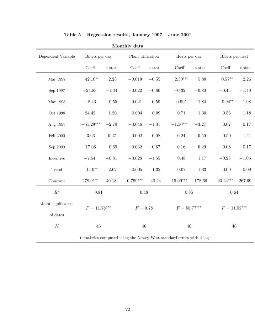
Table 5 �Regression results, January 1997 �June 2001

Monthly data

Dependent Variable Billets per day Plant utilization Heats per day Billets per heat

Coe¤ t-stat Coe¤ t-stat Coe¤ t-stat Coe¤ t-stat

Mar 1997 42:10�� 2:28 �0:019 �0:55 2:30��� 5:89 0:57�� 2:26

Sep 1997 �24:83 �1:34 �0:022 �0:66 �0:32 �0:80 �0:45 �1:49

Mar 1998 �8:43 �0:55 �0:021 �0:59 0:99� 1:84 �0:94�� �1:98

Oct 1998 24:42 1:20 0:004 0:09 0:71 1:30 0:53 1:18

Aug 1999 �51:29��� �2:79 �0:046 �1:31 �1:50��� �3:27 0:07 0:17

Feb 2000 3:63 0:27 �0:002 �0:08 �0:24 �0:50 0:50 1:41

Sep 2000 �17:06 �0:69 �0:032 �0:67 �0:16 �0:29 0:08 0:17

Incentive �7:54 �0:81 �0:028 �1:55 0:48 1:17 �0:28 �1:05

Trend 4:10�� 2:02 0:005 1:32 0:07 1:33 0:00 0:09

Constant 278:9��� 40:18 0:799��� 40:24 15:09��� 178:66 23:24��� 267:69

R2 0:81 0:48 0:85 0:64

Joint signi�cance

of dates

F = 11:78��� F = 0:78 F = 58:77��� F = 11:52���

N 46 46 46 46

t-statistics computed using the Newey-West standard errors with 4 lags

22

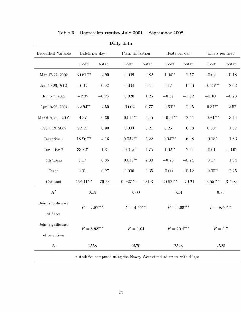
Table 6 �Regression results, July 2001 �September 2008

Daily data

Dependent Variable Billets per day Plant utilization Heats per day Billets per heat

Coe¤ t-stat Coe¤ t-stat Coe¤ t-stat Coe¤ t-stat

Mar 17-27, 2002 30:61��� 2:90 0:009 0:82 1:04�� 2:57 �0:02 �0:18

Jan 19-26, 2003 �6:17 �0:92 0:004 0:41 0:17 0:66 �0:26��� �2:62

Jun 5-7, 2003 �2:39 �0:25 0:020 1:26 �0:37 �1:32 �0:10 �0:73

Apr 19-22, 2004 22:94�� 2:50 �0:004 �0:77 0:60�� 2:05 0:37�� 2:52

Mar 6-Apr 6, 2005 4:37 0:36 0:014�� 2:45 �0:91�� �2:44 0:84��� 3:14

Feb 4-13, 2007 22:45 0:90 0:003 0:21 0:25 0:28 0:33� 1:87

Incentive 1 18:96��� 4:16 �0:032�� �2:22 0:94��� 6:38 0:18� 1:83

Incentive 2 33:82� 1:81 �0:015� �1:75 1:62�� 2:41 �0:01 �0:02

4th Team 3:17 0:35 0:018�� 2:30 �0:20 �0:74 0:17 1:24

Trend 0:01 0:27 0:000 0:35 0:00 �0:12 0:00�� 2:25

Constant 468:41��� 70:73 0:933��� 131:3 20:92��� 79:21 23:55��� 312:84

R2 0:19 0:00 0:14 0:75

Joint signi�cance

of dates

F = 2:87��� F = 4:55��� F = 6:09��� F = 8:46���

Joint signi�cance

of incentives

F = 8:98��� F = 1:04 F = 20:4��� F = 1:7

N 2558 2570 2528 2528

t-statistics computed using the Newey-West standard errors with 4 lags

23

1. Physical investments

Tables 5 and 6 show that some, but not all, of the dummy variables associated with potential

physical investments are signi�cant. For instance, the Mar 1997, Mar 17-27 2002, and Apr

19-22 2004 (the replacement of the EAF transformer) dummies all have a signi�cant positive

e¤ect on billets per day, and all three dummies also have a signi�cant positive e¤ect on heats

per day. In addition, the Mar 1997 and Apr 19-22 2004 dummies also have a signi�cant posi-

tive e¤ect on billets per heat. The Mar 6-Apr 6 2005 (the replacement of the LF transformer)

has a signi�cant positive e¤ect on plant utilization and billets per heat, but a signi�cant neg-

ative e¤ect on heats per day, so overall it does not have a signi�cant e¤ect on Billets per

day.19 Interestingly, the Aug 1999 dummy has a signi�cant negative e¤ect on billets per day

and heats per day. Finally, the F tests shows that combined, the dummies associated with

physical investments had a signi�cant e¤ect in both samples; the only exception is the plant

utilization in Table 5 where the joint e¤ect is not signi�cant.

2. The Incentive scheme

Table 5 shows that the introduction of the incentive scheme in June 2001 had no signi�-

cant e¤ect on output, and if anything, it had a weakly signi�cant negative e¤ect on plant

utilization. One may wonder if this result depends on the fact that the sample in Table 5

ends in June 2001, meaning that we only have one observation (June 2001) on the e¤ect

of the incentive scheme. We therefore rerun the monthly data regressions until the end of

19The negative e¤ect on the Mar 6-Apr 6 2005 dummy on Heats per day seems plausible since an increase in

either kLF or aLF apparently enabled melting more scrap per heat, which is expected to take longer. Indeed,

this event is associated with the main jump in scrap, gas and oxygen per heat (and gas and oxygen per billet)

during the sample, suggesting that more is melted, perhaps for a longer time.

24

2001, so that now we have 7 observations following the introduction of the incentive scheme

(June-December 2001). The results however do not change much and the incentive dummy

remains insigni�cant in all four regression.

By contrast, Table 6 shows that the updates in the incentive scheme had a signi�cant

positive e¤ect on output. This result is mainly due to the increase in heats per day. Indeed, a

main purpose of the incentive scheme is to induce workers to work faster (i.e., induce workers

to �run rather than walk�as management told us), which should boost the number of heats

per day. Interestingly, the updates in the incentive scheme are associated with a decrease in

plant utilization, especially after the �rst update on March 1 2003 (the replacement of the

EAF transformer). It is possible that faster operation leads to more equipment problems

though we do not have direct evidence on that.

3. The 4th team

Table 6 shows that establishing a 4th team in January 2004 had a positive signi�cant e¤ect

on plant utilization, which is reasonable given that the team�s main purpose was to serve as

a backup. The 4th team however does not have a signi�cantly a¤ect billets per day, nor the

other two components of output.

4. Time trend

While Table 4 shows a signi�cant upward time trend in output and its three components,

Tables 5 and 6 show that once we control for the di¤erent events, there is a signi�cant upward

time trend only in the billets per day regression in Table 5 and the billets per heat regression

in Table 6.

25

5. Learning by Doing vs Tweaking

Learning by doing refers to the bene�cial e¤ect of accumulated knowledge on productivity

(Arrow, 1962). Such knowledge is typically modeled as driven by accumulated past output

(e.g., Benkard 2000, Thompson, 2001). We now examine whether productivity gains are in-

deed associated with past accumulated output (irrespective of whether the �rm experimented

with di¤erent production techniques in order to learn how to tweak the production process).

To this end, we de�ne experience �in logs�in period t as the accumulated output up to

period t� 1:

et = log(

t�1X�=1

y� ):

We regress monthly output yt; on et, as well as on all the events reported in Tables 5 and

6. We use monthly data for the entire sample period, since it is unlikely that the melt shop

can learn on a daily basis. Similarly, we de�ne the logged experience of each of the three

components of output (plant utilization, heats per day, and billets per heat) as follows,

ect = log(t�1X�=1

c� ); ct = yh; ht; Ut;

and regress each of the three components, using monthly data on ect , as well as on all the

events.

Tables 7 reports the results of the four regressions in logs, since that is the preferred

speci�cation in the literature, where log experience is used to explain log of output. For the

sake of brevity, we do not report the coe¢ cients on the various events, as we are mainly

interested here in the e¤ect of experience on output and its components (the events are just

used as controls). Since we do not have an experience variable for January 1997, and since

March 1997 is an �event�month with unusually low output level, we start the regression in

April 1997.

26

Table 7 �Regression results on the e¤ect of experience on billets per day and

its decomposition to components

April 1997 - September 2008, Monthly data

Dependent Variable Billets per day Plant utilization Heats per day Billets per heat

Coe¤ t-stat Coe¤ t-stat Coe¤ t-stat Coe¤ t-stat

Experience 0:23 0:47 �0:23 �0:32 0:13 0:31 0:18 0:89

Trend �0:05 �0:08 0:43 0:49 �0:09 �0:17 �0:18 �0:72

Event dummies Yes Yes Yes Yes

R2 0:92 0:63 0:88 0:95

N 126 126 126 126

t-statistics computed using the Newey-West standard errors with 4 lags

Logged experience per se does not help explain the overall growth in the melt shop�s

output, nor the evolution of its three components. When the trend is removed, the coe¢ -

cients of the experience variables become positive, as experience captures the omitted trend:

However, under learning by doing, accumulated experience should explain more than a trend.

Deviations from the trend in experience should be associated with above trend performance.

It does not seem to be the case here.

In sum, the evidence is consistent with the reports from managements, that productivity

gains were the outcome of trail and error, rather than simply a function of accumulated

production.

VI. Decomposing Productivity Gains

We now use the estimated coe¢ cients of the previous regressions to impute the productivity

gains potentially associated with the various events. The coe¢ cient of each dummy represents

27

the gain at the time of the event. By adding all dummies, which we found signi�cantly

di¤erent from 0, we impute all the gains in productivity associated with the events described

in Sections IIIA and IIIB. The remainder, or unexplained, output growth represents the

productivity growth associated with other managerial activities.

The next table presents the change in plant utilization, U , heats per day, h, and billets

per heat, yh, over our sample period.

Table 8 �The change in output components over the sample period:

January 1997 - September 2008, monthly data

y U h yh

Average value Jan 1997 - Dec 1997 320:9 0:7839 17:3 23:60

Average value Jan 2008 - Sep 2008 612:9 0:9603 23:7 26:88

Di¤erence 292 0:1764 6:4 3:28

Di¤erence in percentage terms 91 percent 22:5 percent 37 percent 13:9 percent

Substituting the numbers in Table 8 in (3), we can now decompose the overall increase

in billets per day over the sample period as follows:

(1 + dU)(1 + dh)(1 + dy) = 1:225� 1:37� 1:139 = 1:91: (4)

Let us �rst consider physical investments. The sum of the signi�cant date dummies, those

associated with potential plant shut downs for investments, represent a total decrease of 9:19

tons of billets per day (42:10�51:29) during the �rst period, and an increase of 53:54 tons of

billets per day (30:61 + 22:94) during the second part of the sample. In total then, the date

dummies can explain an increase of 44:36 tons of billets per day, out of the total increase of

292 tons of billets per day. This amounts to 15:2 percent of the total increase.

28

Looking at the di¤erent components in Tables 5 and 6, we see that the physical invest-

ments increased output primarily by increasing heats per day (the signi�cant date dummies

amount to 2:50 heats per day out of the total increase of 6:4) and billets per heat (the signif-

icant date dummies amount to 0:91 billets per heat out of the total increase of 3:28), while

having only a small e¤ect on plant utilization (the signi�cant date dummies amount to 0:014

out of the total increase of 0:1764).

Second, the incentive scheme has a signi�cant e¤ect on billets per day only in Table 6,

where combined, the two incentive dummies are associated with increases of 52:77 tons of

billets per day (18:96+33:82), which amounts to 18:1 percent of the total increase of 292 tons

in billet per day. Table 6 shows that the gains come mostly from the positive e¤ect on heats

per day (the signi�cant incentive dummies amount to 2:55 heats per day out of the total

increase of 6:4). The e¤ect on billets per heat is small (the signi�cant incentive dummies

amount to 0:18 billets per heat out of the total increase of 3:28), while, surprisingly, the e¤ect

on plant utilization is negative (the signi�cant incentive dummies amount to �0:047). Finally,

the 4th team dummy only has a statistically signi�cant e¤ect only on plant utilization.

In total, the explained components amount to 97:13 of daily output growth, which repre-

sent a third of total increase of 292 tons of billets per day during the sample period.20 The

remaining growth of 194:8 tons of billets per day (292� 97:13), which is left unexplained by

the investments and the incentive scheme, represents 66:7 percent of the total growth, and

amounts to annual growth of 4:12 percent ((1 + 194:8=320:9)1=11:67 � 1).20 Interestingly, if we also take into account all the jointly signi�cant dummies (the investment dummies in

the Billets per day, Heats per day, and Billets per heat regressions in Table 5 and all the investments dummies

in Table 6), we either get very similar, or even smaller explained growth, because many of the dummies in

Tables 5 and 6 which are jointly, but not individually, signi�cant, have negative coe¢ cients.

29

Another way to measure productivity, is to look at the evolution of value added instead

of gross output. We de�ne value added, at constant prices, as:

V A = pyy �nXi=1

pixi;

where y represents the output of billets, py is the average price of billets over the sample

period, x1; : : : ; xn is a vector of material and energy inputs, including scrap, electricity, Ferro

alloys, Oxygen, Propane, Lime, electrodes and Carbon, and pi is the average price of input i

over the sample period. We use constant prices in order to ensure that value added re�ects

changes of physical units, as opposed to changes in the relative prices of inputs and output;

for instance, if billet prices increased more than input prices, value added would increase for

reasons which are unrelated to productivity.

Since capital and labor were more or less constant over the sample period (save for the

events), we can think of the growth in V A as a measure of the evolution of capital and labor

productivity. Loosely speaking, TFP can be de�ned as V A=(pkK + pLL), where pkK and

pLL are the values of capital and labor inputs, measured in constant prices. In our case,

both K and L were �xed over the sample period (up to the events), so the evolution of V A

can be interpreted as a proxy for TFP.

Value added increased from 1997 to 2008 by 63:7 percent. In the Appendix, we report the

results of a regression of V A on all the events, using monthly data. The results show that the

events explain only 38:3 percent of the increase in V A. The remaining 61:7 percent remain

unexplained. The unexplained growth in V A amounts to an annual productivity growth of

3:06 percent:

30

VII. Discussion and Conclusions

This study documents the evolution of productivity in a �rm operating in a traditional, ma-

ture, industry. Despite the absence of dramatic changes in the plant itself or the workforce,

output increases gradually and continuously throughout the sample period. While an in-

centive scheme and some investments explain part of the gains in the di¤erent components

of output, we are left with most of the gain unexplained. This gain is also not explained

by cumulative experience, as one would expect based on standard learning by doing model.

Moreover, the gain cannot be explained by R&D as the �rm we study uses standard equip-

ment which cannot be modi�ed by the �rm itself.21

Learning by experimenting, or �tweaking the production process,� is the best explana-

tion we gather from conversations with management. As it turns out, steel production in

mini mills involves numerous trade-o¤s. For instance, using more refractories (non-metallic

materials that line the EAF�s shell and protect it from melting), allows the melt shop to run

more heats before the refractories need to be replaced, but at the same time, it limits the

amount of scrap that can be charged into the EAF, and hence the quantity of billets per heat.

Likewise, using a longer electric arc allows the melt shop to reach higher temperatures inside

the EAF and thereby speeds up the heat cycles, but may damage the refractories and requires

the melt shop to replace them sooner (replacing the refractories requires a downtime). As a

third example, charging more scrap into the EAF, increases the quantity of billets per heat,

but can also raise the probability that the electrodes (that strike the electric arc inside the

EAF) will break, in which case the melting process needs to be stopped until the electrodes

21 In an interview, the steelmaker�s CEO said �in the steel industry you cannot invent anything. You must

use the equipment according to the manufacturer�s speci�cations.�Interestingly, when early on the steelmaker

tried to improve on the way baskets of scrap are charged into the EAF, the experiment has ended in an accident.

31

are replaced. Finding the optimal balance between the various trade-o¤s requires a lengthy

trail and error process that can be very slow, given that there are many variables that may

a¤ect the various trade-o¤s. Moreover, these variables di¤er across melt shops, even if they

are all using the same equipment. The implication is that �learning how to use the melt shop

optimally,� or �tweaking the production process� is a slow process that involves numerous

trade-o¤s and can take a long time.

Beyond their theoretical and empirical relevance, our �ndings imply that learning by

doing is not simply a function of cumulative output and is not guaranteed automatically.

Rather, it is the result of an active experimentation process. Of course, our results re�ect the

learning process at one particular plant, in one particular industry. In this sense, our study

shares the issue of generalizability with most of the rest of the learning-by-doing literature.

Nevertheless, we believe that the �ndings o¤er insights that can be cautiously extended to

other production operations, particularly complex manufacturing processes.

32

References

[1] Arrow, Kenneth J. 1962. �The Economic Implications of Learning By Doing.�Review

of Economic Studies 29: 155-173.

[2] Asker, John, Allan Collard-Wexler, and Jan De Loecker. 2012. �Productiv-

ity Volatility and the Missallocation of Resources in Developing Economies.�

http://pages.stern.nyu.edu/~acollard/Productivity_Volatility_Misallocation.pdf

[3] Bartel, Ann, Richard Freeman, Casey Ichniowski, Morris Kleiner. 2011. �Can a Work-

place Have an Attitude Problem? Workplace E¤ects on Employee Attitudes and Orga-

nizational Performance,�Labour Economics. 18(4): 411�423.

[4] Benkard, Lanier C.. 2000. �Learning and Forgetting: The Dynamics of Aircraft Produc-

tion.�American Economic Review 90(4): 1034-1054.

[5] Bessen, James. 2003. �Technology and Learning by Factory Workers: The Stretch Out

at Lowell, 1842.�The Journal of Economic History. 63(1): 33-64.

[6] Boning, Brent., Casey Ichniowski, and Kathryn Shaw. 2007. �Opportunity Counts:

Teams and the E¤ectiveness of Production Incentives.� Journal of Labor Economics,

25(4): 613-650.

[7] Collard-Wexler, Allan., and Jan De Loecker. 2012. �Reallocation and Technology: Evi-

dence from the U.S. Steel Industry.�Mimeo

[8] Das, Sanghamitra, Kala Krishna, Sergey Lychagin, and Rohini Somanathan. 2012. �Back

on the Rails: Competition and Productivity in State-owned Industry.� Forthcoming,

AEJ Applied.

33

[9] Fisher, Franklin., John J. McGowan and Joen E. Greenwood. 1983. Folded, Spindled

and Mutilated: Economic Analysis and US vs. IBM, Cambridge, Mass.: MIT Press

[10] Genberg, Mats. 1992. �The Horndal E¤ect: Productivity Growth without Capital In-

vestments at Horndalsverken During 1927 and 1952.�Department of Economic History,

University of Uppsala, Sweden.

[11] Ghemawat, Pankaj. 1995. �Competitive Advantage and Internal Organization: Nucor

Revisited,�Journal of Economics & Management Strategy. 3(4): 685-717.

[12] Griliches, Zvi. 1996. �The Discovery of the Residual: A Historical Note.� Journal of

Economic Literature. 34(3): 1324-1330.

[13] Ichniowski, Casey and Kathryn Shaw. 2003. �Beyond Incentive Pay: Insiders�Estimates

of the Value of Complementary Human Resource Management Practices.� Journal of

Economic Perspectives. 17(1): 155-80.

[14] Lazonick, William and Thomas Brush. 1985. �The �Horndal E¤ect�in Early U.S. Man-

ufacturing.�Explorations in Economic History. 22: 53-96.

[15] Levitt, Steven, John List, and Chad Syverson. 2012. �Toward an Understanding of

Learning by Doing: Evidence from an Automobile Assembly Plant.�Mimeo.

[16] Lundberg, Erik. 1961. Produktivitet och Räntabilitet. Stockholm: Norstedt & Saner.

[17] Meisenzahl, Ralf R., and Joel Mokyr. 2012. �The Rate and Direction of Invention in the

British Industrial Revolution: Incentives and Institutions,� In Lerner J. and S. Stern

(Eds.), The Rate and Direction of Inventive Activity Revisited. Chicago: University of

Chicago Press, 443-479.

34

[18] Mokyr, Joel 1990. The lever of Riches: Technological creativity and economic progress,

Oxford University Press.

[19] Scherer, Frederic M. 1996. Industry Structure, Strategy, and Public Policy, Harper

Collins College Publishers.

[20] Syverson, Chad. 2011. �What Determines Productivity?�Journal of Economic Litera-

ture. 49(2): 326�365.

[21] Thompson, Peter. 2001 �How Much Did the Liberty Shipbuilders Learn? New Evidence

for an Old Case Study,�Journal of Political Economy. 109(1): 103-137.

[22] Tether, Bruce. and Stan Metcalfe (2003), �Horndal at Heathrow? Capacity Creation

through Cooperation and System Evolution.� Industrial and Corporate Change. 12(3):

437-476.

35

VIII. Appendix

Work Hours and Wage Premium Total monthly work hours (regular work hours plus

overtime) are presented in the following �gure. We have data on monthly work hours only

for a part of the entire sample period.

0

5000

10000

15000

20000

25000

Jan­01 Jul­01 Feb­02 Sep­02 Mar­03 Oct­03 Apr­04 Nov­04 May­05

Month

Tota

l wor

k ho

urs

Figure A1: Total work hours, January 2001 - July 2005

The �gure shows clearly that monthly work hours remained pretty much constant. It

is interesting to note that during the period covered by the �gure, the output of billets has

increased from an average level of 13; 957 tons per month in 2001 to an average level of 16; 464

tons per month in 2005, which re�ects an increase of 18 percent in output.

The following �gure shows the total wage premium that was paid to workers above their

base salary:

36

10%

20%

30%

40%

50%

60%

70%

80%

Jan­01 May­02 Oct­03 Feb­05 Jul­06 Nov­07

Year

Ince

ntiv

e pa

ymen

t

Figure A2: Wage premium paid to employees, 2001-2008

The �gure shows an upward trend in incentive payments from around 35 percent of base

salary in 2001, when the incentive scheme was just introduced to around 60 percent towards

the end of the sample period in 2008, though there is considerable variability of incentive

payments around the upward trend line. In fact, the standard deviation of incentive payments

around their mean is 64 percent higher in 2005� 2008 than in 2001� 2004.

Another interesting question to ask is how frequently did the workers meet the predeter-

mined thresholds in the incentive scheme? To answer this question, let b denote the average

production of billets in tons per e¤ective plant hour in a given day and recall from Table

3 that the incentive scheme speci�es three thresholds on b: Q0, Q1, Q2. Workers receive a

bonus w1 if Q0 � b � Q1, a bonus w2 if Q1 � b � Q2. The bonus is maxed out at Q2, and

no bonus is paid if b < Q0. In the next �gure we show the distribution of b for each month

from July 2001 to September 2008.22

22Although the incentive scheme starts on June 2001, we do not have daily data on June 2001..

37

0%

10%

20%

30%

40%

50%

60%

70%

80%

90%

100%

Jul­0

1

Nov­01

Mar­02

Jul­0

2

Nov­02

Mar­03

Jul­0

3

Nov­03

Mar­04

Jul­0

4

Nov­04

Mar­05

Jul­0

5

Nov­05

Mar­06

Jul­0

6

Nov­06

Mar­07

Jul­0

7

Nov­07

Mar­08

Jul­0

8

b < Q0 Q0 < b < Q1 Q1 < b < Q2 b > Q2

Figure A3: The distribution of the daily average production of tons of

billets per e¤ective plant hour, b, for each month, July 2001-

September 2008

As the �gure shows, about 60 percent of the time, b was between Q1 and Q2. It exceeded

Q2 about 16 percent of the time (though more frequently in later periods), and fell short of

Q0 only 6 percent of the time. In the next Table we summarize the distribution of b for the

di¤erent time periods (before and after the incentive scheme was revised).

Table A1 �The distribution of b

Dates b < Q0 Q0 � b � Q1 Q1 � b � Q2 b > Q2

July 1, 2001 - March 1, 2003 8:2 percent 16:3 percent 72:7 percent 2:7 percent

March 1, 2003 - July 1, 2005 7:5 percent 17:1 percent 62:5 percent 12:8 percent

July 1, 2005 - September 28, 2008 4:5 percent 14:6 percent 54:0 percent 26:8 percent

July 1, 2001 - September 28, 2008 6:3 percent 15:8 percent 61:1 percent 16:8 percent

38

One can see that over time, b was much more likely to exceed Q2, which the upper

threshold on the incentive scheme: while in the �rst period b was above Q2 in only 2:7

percent of the cases, it was above Q2 in close to 27 percent of the cases in the last part of the

sample. Moreover, cases where b fell short of Q0, which is the lower threshold above which the

workers start getting a bonus, fell from 8:2 percent at the �rst period to 4:5 percent during

the last period of the sample. In general, the distribution in the last period stochastically

dominates the distribution in the second period and the �rst period. This explain why the

total incentive payments trended up as we saw earlier.

6. Pro�tability

One may argue that a possible reason why we see increase in productivity is that the price of

billets and rebars increased dramatically just before the global �nancial crisis in September

2008 and hence, the melt shop found it pro�table to expand output while beforehand it did

not work at full capacity not because it was unable to do that but rather because it did not

�nd it pro�table to do so. Interviews with the steelmaker�s management reveal that was not

the case: the melt shop was trying to operate at full capacity from the day the current owner

acquired the melt shop at least until September 2008, and the only impediment to production

expansion was the e¤ective capacity of the melt shop, which was limited, but kept increasing

over time in the way we document in this paper.

Still, one may wonder if production was pro�table or not. To examine this issue, we com-

pute the direct pro�tability of billet production, de�ned as the international price of billets

as quoted in Metal Bulletin, times the monthly production of billets, net of the variable cost

of billets, including the price of scrap, electricity, Carbon, Lime, Ferro alloys, etc. (directly

pro�tability is in fact similar to the concept of value added except that it is expressed in

39

terms of current rather than constant prices). The computation shows that the direct prof-

itability of billets production was positive until the eruption of the global �nancial crisis at

the end of 2008. This �nding is consistent with the management�s claim that it was had an

incentive to expand output as much as possible. The implication then is that the constraint

on production was technical, rather than a deliberate restraint on output by management.

The puzzle is how did the steelmaker manage to expand output, and given that this was

pro�table all along, why wasn�t it done earlier?

7. Delays

One of the important determinants of productivity are various delays and problems in the

production process. In the following �gure we present some of the delays and problems over

the period August 2001- September 2001. The delays and problem that we report are in

loading the scrap into the EAF (scrap leveling and scrap waiting delays), problems with

electricity and electrodes, problems with the ladle furnace, delays when pouring the molten

steel from the EAF to the ladle furnace (tapping delays), delays due to the need to repair

damages to the refractories which line the EAF�s shell and protect it from melting, and total

delays.

40

Scrap leveling delays

0

5

10

15

20

Aug­01 Aug­02 Aug­03 Aug­04 Aug­05 Aug­06 Aug­07 Aug­08

Month

Min

utes

 per

 day

Scrap waiting  delays

0

5

10

15

20

Aug­01 Aug­02 Aug­03 Aug­04 Aug­05 Aug­06 Aug­07 Aug­08Month

Min

utes

 per

 day

Electrodes change delays

0

5

10

15

20

25

30

35

Aug­01 Aug­02 Aug­03 Aug­04 Aug­05 Aug­06 Aug­07 Aug­08Month

Min

utes

 per

 day

Electricity problems

0

5

10

15

20

25

30

35

40

45

50

Aug­01 Aug­02 Aug­03 Aug­04 Aug­05 Aug­06 Aug­07 Aug­08Month

Min

utes

 per

 day

Laddle problems

0

2

4

6

8

10

Aug­01 Aug­02 Aug­03 Aug­04 Aug­05 Aug­06 Aug­07 Aug­08

Month

Min

utes

 per

 day

Tapping delays

0

10

20

30

40

50

60

70

80

90

100

110

Aug­01 Aug­02 Aug­03 Aug­04 Aug­05 Aug­06 Aug­07 Aug­08

Month

Min

utes

 per

 day

Fettling delays

0

10

20

30

40

Aug­01 Aug­02 Aug­03 Aug­04 Aug­05 Aug­06 Aug­07 Aug­08Month

Min

utes

 per

 day

Total delays

0

50

100

150

200

250

300

Aug­01 Aug­02 Aug­03 Aug­04 Aug­05 Aug­06 Aug­07 Aug­08

Month

Min

utes

 per

 day

Figure A4: Average delays and problems in minutes per day, August

2001-September 2008

The �gure shows that delays due to feeding the scrap into the EAF were cut signi�cantly

in 2004: Electricity problems, Ladle problems, and fetling delays also show a decreasing trend

although these trends seem to be less dramatic than the decrease in scarp related delays. On

the other hand, the need to change electrodes led to increasing delays as production grew

over time, and tapping delays also show an increasing trend with a temporary decrease in

2003�2004. The �nal �gure shows that total delays grew somewhat over time as production

increased.

41

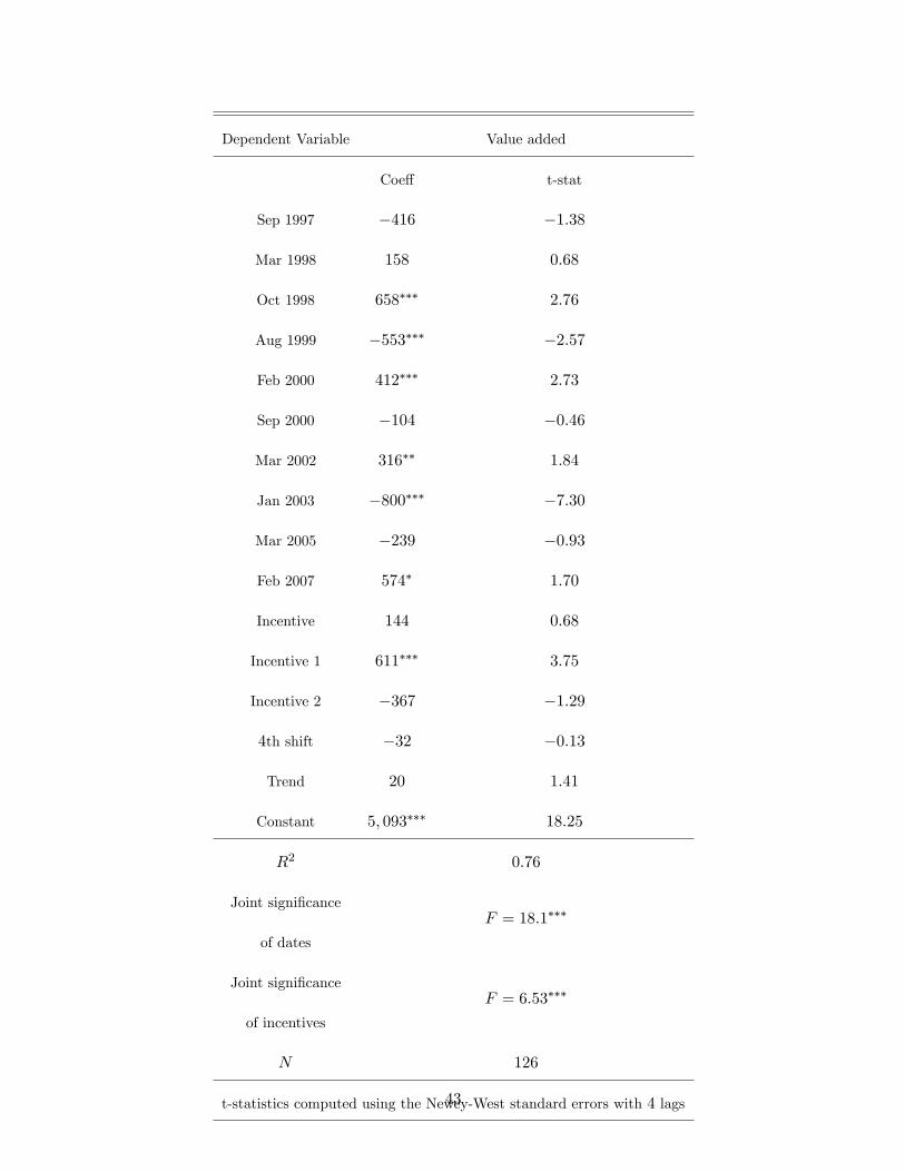
8. Value added

Value added in constant prices is computed for each period by multiplying the quantity of

billets and the quantity of inputs by their respective average prices over the entire sample

period. The price of billets is the international price published in Metal Bulletin (the steel-

maker consumes all billets in its rolling mill and does not sell them on the market). We than

regressed value added on the same dummies that were used in Tables 5 and 6. Due to missing

observations in January 1997 and since March 1997 is an �event�month with an unusually

low output level, the regression starts from April 1997.

Table A2 �Value Added regression, April 1997 �September 2008

Monthly data

42

Dependent Variable Value added

Coe¤ t-stat

Sep 1997 �416 �1:38

Mar 1998 158 0:68

Oct 1998 658��� 2:76

Aug 1999 �553��� �2:57

Feb 2000 412��� 2:73

Sep 2000 �104 �0:46

Mar 2002 316�� 1:84

Jan 2003 �800��� �7:30

Mar 2005 �239 �0:93

Feb 2007 574� 1:70

Incentive 144 0:68

Incentive 1 611��� 3:75

Incentive 2 �367 �1:29

4th shift �32 �0:13

Trend 20 1:41

Constant 5; 093��� 18:25

R2 0:76

Joint signi�cance

of dates

F = 18:1���

Joint signi�cance

of incentives

F = 6:53���

N 126

t-statistics computed using the Newey-West standard errors with 4 lags43

The total increase in value added from 1997 to 2008 was 3; 181, from an average of 4; 992

in 1997 (April till December) to an average of 8; 173 in 2008 (January till September). Since

the sum of the signi�cant date dummies is 606, while the sum of the incentive dummies is 611,

combined, physical investments and incentives explain 38:2 percent of the increase in value

added over the sample period. The remaining 61:7 percent or 1; 964, remain unexplained and

amount to an annual growth rate of 3:06 percent ((1 + 1; 964=4; 992)1=11 � 1).

44