Resonanceofatension legplatformexitedby third...

rsta.royalsocietypublishing.org

ResearchCite this article: Zhou BZ, Wu GX. 2015Resonance of a tension leg platform exited bythird-harmonic force in nonlinear regularwaves. Phil. Trans. R. Soc. A 373: 20140105.http://dx.doi.org/10.1098/rsta.2014.0105

One contribution of 12 to a Theme Issue‘Advances in fluid mechanics for offshoreengineering: a modelling perspective’.

Subject Areas:ocean engineering

Keywords:tension leg platform, third-harmonicresonance, floating body/wave interaction,fully nonlinear theory, higher order boundaryelement method

Author for correspondence:G. X. Wue-mail: [email protected]

†Present address: Department of MechanicalEngineering, University College London,Torrington Place, LondonWC1E 7JE, UK.

Resonance of a tensionleg platform exited bythird-harmonic forcein nonlinear regular wavesB. Z. Zhou and G. X. Wu†

College of Ship Building Engineering, Harbin Engineering University,Harbin 150001, People’s Republic of China

The resonance of a floating tension leg platform(TLP) excited by the third-harmonic force of aregular wave is investigated based on fully nonlineartheory with a higher order boundary element method(BEM). The total wave elevation and the totalvelocity potential are separated into two parts,based on the incoming wave from infinity andthe disturbed potential by the body. A numericalradiation condition is then applied at the far fieldto absorb the disturbed potential without affectingthe incident potential. The BEM mesh on the freesurface is generated only once at the initial timeand the element nodes are rearranged subsequentlywithout changing their connectivity by using a springanalysis method. Through some auxiliary functions,the mutual dependence of fluid/structure motionsis decoupled, which allows the body acceleration tobe obtained without the knowledge of the pressuredistribution. Numerical simulation is carried out forthe interaction of a floating TLP with waves. Thefocus is on the motion principally excited by higherharmonic wave forces. In particular, the resonance ofthe ISSC TLP generated by the third-order force at thetriple wave frequency in regular waves is investigated,together with the tensions of the tendons.

1. IntroductionRinging in the offshore industry usually refers tothe transient response of a platform at frequenciesmuch higher than the dominant component of theincoming wave. It is commonly shown by certain kindsof offshore structures such as tension leg platforms(TLPs) and gravity-based structures (GBSs) and has

2014 The Author(s) Published by the Royal Society. All rights reserved.

on September 8, 2018http://rsta.royalsocietypublishing.org/Downloaded from

http://crossmark.crossref.org/dialog/?doi=10.1098/rsta.2014.0105&domain=pdf&date_stamp=2014-12-15

mailto:[email protected]

http://rsta.royalsocietypublishing.org/

2

rsta.royalsocietypublishing.orgPhil.Trans.R.Soc.A373:20140105

.........................................................

been a major concern to operators and engineers since it was first observed in a model test of theHutton TLP in the North Sea [1]. TLPs are generally designed to keep their natural frequenciesin heave, pitch and roll degrees of freedom, several times above the dominant wave frequency,whereas natural frequencies in surge, sway and yaw degrees of freedom are designed to be lowerthan the dominant wave frequency. A report [2] funded by the UK Health and Safety Executive,addressed the ringing of a typical GBS with multiple-columns, which has its natural frequencywell above the dominant wave frequency. Although TLPs and GBS with this kind of designavoid the linear resonance, ringing becomes important when the range of natural frequencyis several times higher than the dominant wave frequencies. Typically when a transient wavepasses through the platform, the structure will continue to oscillate over a period of time at itshigh natural frequency even when the wave excitation has diminished. This oscillation can bepersistent when the damping level is low. Understanding of such ringing behaviour is importantbecause of the high level of stress generated.

A closely related problem is springing, which usually refers to the resonant response of aplatform in a stochastic sea state, when the stochastic properties of the motion have becomesteady. It is highly relevant to the fatigue analysis of the structure. As the natural frequency ofa TLP or GBS is high, such resonance is unlikely to be excited by the linear force at the dominantfrequency ω of the wave spectrum and it is more likely to be excited by the nonlinear force atnω, n = 2, 3, . . .. It is then evident that both ringing, the transient response, and springing, thesteady response in the stochastic sense, are principally due to the higher harmonic components ofthe nonlinear wave force. Thus in the present work, we will consider the resonant behaviour of aTLP platform excited by the higher harmonic force of a regular wave. Although the regular wavemay not truly reflect the stochastic nature of the real sea state, the results obtained can providesome insight into the ringing and springing behaviours of the platform. In particular, we shall usethe high-order Stokes wave as the incoming wave together with the fully nonlinear analysis. Themain frequency of the Stokes wave may be away from the high natural frequency of the structure,but the higher frequencies in its higher order terms can be close to the natural frequency. However,the significance of the higher modes diminishes gradually in moderately steep waves. As a result,resonant response of a structure typically occurs when its natural frequency is about three to fivetimes the incoming wave frequency, or it is most likely to be excited by the third-order force atthe triple wave frequency.

Extensive effort has been made previously to improve the understanding of the ringing andspringing related to the high-frequency response and to develop numerical tools to improve thedesign. The Norwegian Petroleum Directorate and the UK Health and Safety Executive jointlyfunded a project named ‘Higher order wave load effects on large volume structures’ in 1993 [3],which focused on a series of field observations, experimental models and numerical simulationresearch of TLPs and GBS, and produced some very valuable results. Petrauskas & Liu [4] carriedout two model tests on springing, one measuring springing forces on a vertical cylinder and theother measuring the response of a TLP. Extensive experiments have also been conducted to studythe ringing phenomenon with a circular cylinder in the wave tank [5–7]. Kim et al. [8] and Zou et al.[9] also carried out the experiment with a model of the ISSC TLP to measure the force and thenobtained the response of the platform through equations of motion. In the simulations, while thereis work based on empirical equations [10], most research on higher order loads is based on theperturbation theory up to the third order. Typical examples include that by Faltinsen et al. [11] fora slender cylinder in long waves and that by Malenica & Molin [12] for a cylinder in finite waterdepth. Teng & Kato [13] also calculated the third-order wave load at the triple wave frequency onfixed axisymmetric bodies by monochromatic waves. We may note that the perturbation theory isvalid only for moderate waves. In deep seas, an offshore structure is designed to operate in a veryhostile environment. A more rational approach would be to adopt the fully nonlinear theory.

Much of the work on fully nonlinear wave interactions with three-dimensional structures isbased on a numerical wave tank with a wave maker on one side and an absorbing beach onthe other side. Wu & Hu [14], Wang et al. [15] and Yan & Ma [16] adopted this model withthe finite-element method, while Liu et al. [17], Bai & Eatock Taylor [18] and Yan & Liu [19]



3


.........................................................

d

y z

x

n

SD

SF

SB

y¢

o¢x¢

z¢

o

S• S•

Figure 1. Sketch of coordinate systems and computation domain.

used the model with the boundary element method (BEM). While this numerical tank reflectsexperimental practice well, it has similar problems to a physical tank when modelling the trueocean environment in the open sea, because of the way in which the wave is generated and theside wall effect. Ferrant [20] proposed a model for the open sea, in which the total potential is splitinto the incident potential and the disturbed potential. A model similar to this has been used byFerrant [21], Ferrant et al. [22], Ducrozet et al. [23] and Shao & Faltinsen [24].

In this work, we adopt the technique of Ferrant [20] to split the total potential. It attempts toinvestigate high-frequency resonance during wave interaction with an ISSC TLP by employingthe fully nonlinear time domain numerical model in the open sea developed by Zhou et al. [25].The adopted numerical model is verified by comparing the surge added mass of the TLP with thelinear frequency-domain results, as well as by comparing amplitudes and phases of the first fourharmonic forces on a fixed vertical cylinder with experimental data and other nonlinear numericalresults. Numerical simulations are then carried out by setting the triple wave frequency at/closeto the natural frequency of the TLP in the pitching mode. Comparison with the results for thebody in a single degree of freedom is made to illustrate the coupling effects of the motion indifferent modes. Numerical results for the motions and tensions of the tendons are presented.In addition, a harmonic analysis of the time history of the fully nonlinear results is performed,from which the importance of higher order effects can be identified. Moreover, the effects ofwave frequency on motions in the heave and pitch modes and on the tension of the tendonare analysed.

2. Mathematical model and numerical procedure

(a) Mathematical modelThe problem of wave interaction with a TLP in an open sea with water depth d is sketchedin figure 1. Two right-handed Cartesian coordinate systems are defined. One is a space-fixedcoordinate system oxyz with the oxy plane on the undisturbed free surface and with the z-axisbeing positive upwards. The other is a body-fixed coordinate system o′x′y′z′ with its origin o′placed at the centre of mass of the body. When the body is at its equilibrium position, thesetwo sets of coordinate systems are parallel to each other. The centre of mass is located initiallyat Xc0 in the space-fixed coordinate system, and Xc = Xc0 + ζ subsequently. Here, ζ = (ζ1, ζ2, ζ3)is introduced to denote the translational displacements of the mass centre in the x-, y- andz directions, respectively. The rotation of the body is defined through the usual Euler anglesθ = (α,β, γ ) = (ζ4, ζ5, ζ6) to illustrate the displacements in roll, pitch and yaw, the terms commonlyused in the naval architecture.



4


.........................................................

Based on the assumption that the fluid is ideal and incompressible, and flow is irrotational, thevelocity potential φ(x, y, z, t) can be introduced, which satisfies the Laplace equation in the fluiddomain R

∇2φ = 0. (2.1)

On the instantaneous free water surface SF, the fully nonlinear kinematic and dynamic boundaryconditions can be given in the following Lagrangian form:

DXDt

= ∇φ (2.2)

andDφDt

= −gη + 12∇φ · ∇φ, (2.3)

where g represents the acceleration due to gravity, X = (x, y, z) denotes the position vector of afluid particle on the free surface, η is the elevation of water surface measured from its meanlevel, D/Dt = ∂/∂t + u · ∇ is the total derivative with u being the velocity of the fluid particle. Theboundary condition on the body surface SB is

∂φ

∂n= V · n, (2.4)

where V is the velocity of the body surface, n is the normal of the surface pointing out of the fluiddomain, as shown in figure 1. The body surface velocity can be expanded as

V = U + Ω × rb, (2.5)

where rb = X′ is the position vector in the body-fixed coordinate system, U = (U1, U2, U3) is thetranslational velocity of the centre of mass, Ω = (U4, U5, U6) is the rotational velocity, which canbe linked to the variation of the Euler angles [26].

Similar to Ferrant [20], the total wave elevation and the total velocity potential on the freesurface can be separated arbitrarily into two parts, which can be written as

η(x, y, t) = ηa(x, y, t) + ηb(x, y, t) (2.6)

and

φ(x, y, η(x, y, t), t) = φa(x, y, η(x, y, t), t) + φb(x, y, η(x, y, t), t). (2.7)

The total wave and potential should tend to the incident wave and potential at infinity. This canbe achieved if we let

ηa → 0; φa → 0 r → ∞ (2.8)

and

ηb → ηI; φb → φI r → ∞, (2.9)

where r =√

x2 + y2. Provided equations (2.8) and (2.9) are satisfied, there is no restriction on theirindividual choice. Thus, when the analytical solution is available for ηI and φI, such as the higherorder Stokes waves, they can be the foundation for the choice of (φb, ηb). We write

ηb(x, y, t) = ηI(x, y, t) (2.10)

and

φb(x, y, η(x, y, t), t) = φI(x, y, η(x, y, t), t). (2.11)

We note that the analytical expression for φI is for z ≤ ηI. When z = η in equation (2.11) is beyondthis region, the potential is no longer the originally defined incident potential. In other words,φb strictly speaking is not the incident potential without the body. It has a contribution from thebody due to the change in the wave elevation.



5


.........................................................

Substituting equations (2.6), (2.7), (2.10) and (2.11) into the governing equation and boundaryconditions for φ, we obtain the following governing equation and the free surface boundaryconditions of the boundary value problem for (φa, ηa):

∇2φa = 0 in R, (2.12)

DxDt

= ∂φa

∂x+ ∂φb

∂xon SF, (2.13)

DyDt

= ∂φa

∂y+ ∂φb

∂yon SF, (2.14)

Dηa

Dt= ∂φa

∂z+ ∂φb

∂z− ∂ηb

∂t− ∇φb · ∇ηb − ∇φa · ∇ηb on SF (2.15)

andDφa

Dt= −g(ηb + ηa) − ∂φa

∂t+ 1

2|∇φa|2 − 1

2|∇φb|2 on SF. (2.16)

An artificial damping zone is applied on the outer annulus of a circular computational domain toabsorb the scattered wave. In this study, both φ- and η-type damping terms are added to the freesurface conditions in equations (2.13)–(2.16) [25].

On the body surface SB, the boundary condition for φa is

∂φa

∂n= V · n − ∂φb

∂n. (2.17)

To complete the boundary value problem, the initial conditions on the free surface can be given as

{φa = 0 z = ηb

ηa = 0t = 0. (2.18)

In order to avoid an abrupt start and allow a gradual development of the body motion anddisturbed potential, all the terms involving ηb and φb are multiplied by a modulation function.

In this study, the fifth-order Stokes wave [27] is used as the incoming wave, with the waveamplitude A being defined as half of the wave height or distance between wave peak and trough.Although the fifth-order incident wave does not satisfy the fully nonlinear free surface conditionexactly, it is expected to be a good approximation for the fully nonlinear theory and can provideaccurate results for the resonant behaviour driven principally by the third-harmonic force.

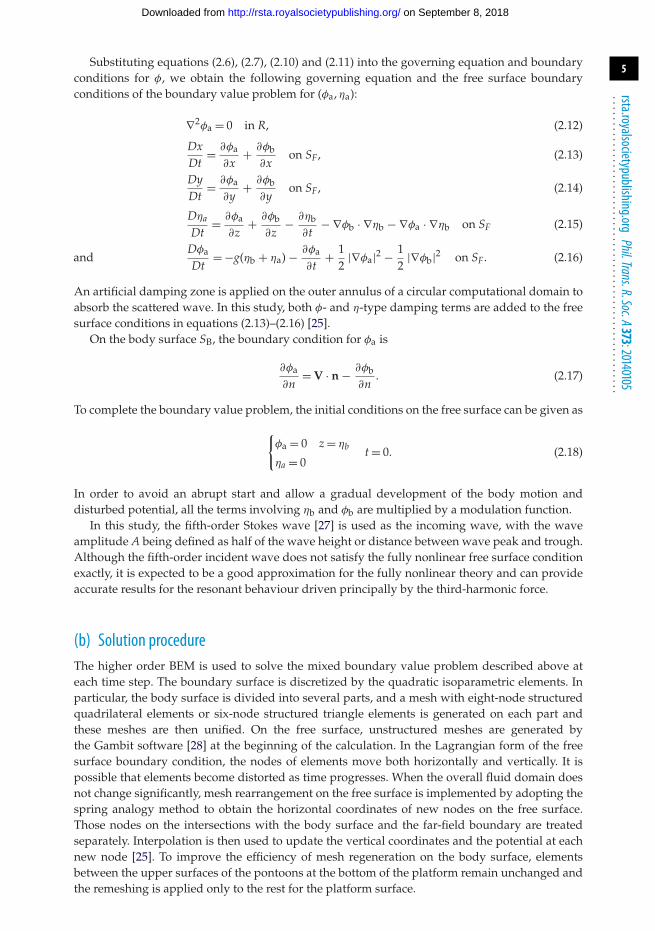
(b) Solution procedureThe higher order BEM is used to solve the mixed boundary value problem described above ateach time step. The boundary surface is discretized by the quadratic isoparametric elements. Inparticular, the body surface is divided into several parts, and a mesh with eight-node structuredquadrilateral elements or six-node structured triangle elements is generated on each part andthese meshes are then unified. On the free surface, unstructured meshes are generated bythe Gambit software [28] at the beginning of the calculation. In the Lagrangian form of the freesurface boundary condition, the nodes of elements move both horizontally and vertically. It ispossible that elements become distorted as time progresses. When the overall fluid domain doesnot change significantly, mesh rearrangement on the free surface is implemented by adopting thespring analogy method to obtain the horizontal coordinates of new nodes on the free surface.Those nodes on the intersections with the body surface and the far-field boundary are treatedseparately. Interpolation is then used to update the vertical coordinates and the potential at eachnew node [25]. To improve the efficiency of mesh regeneration on the body surface, elementsbetween the upper surfaces of the pontoons at the bottom of the platform remain unchanged andthe remeshing is applied only to the rest for the platform surface.



6


.........................................................

(c) Hydrodynamic forces and body motionsThe equation of motions for a rigid body can be written as [26]

[M]U̇ = Fh + Fe (2.19)

and

[I]Ω̇ + Ω × [I]Ω = Nh + Ne, (2.20)

where U and Ω are defined after equation (2.6), and U̇ = [a1, a2, a3]T and Ω̇ = [a4, a5, a6]T indicatethe translational acceleration and the angular acceleration, respectively. [M] and [I] in theequations are mass and rotational inertia matrixes, and Fe = [fe1, fe2, fe3]T and Ne = [fe4, fe5, fe6]T

are the external force and moment about the centre of mass. As the rotational centre is at thecentre of the body mass, there is no coupling between translational and rotational motions onthe left-hand sides of equations (2.19) and (2.20). However, the coupling does exist implicitlyon the right-hand sides. The hydrodynamic force Fh = (f1, f2, f3) and moment Nh = (f4, f5, f6) onthe body can be obtained by integrating the pressure over its wetted surface

fi = −ρ∫∫

SB

(∂φ

∂t+ 1

2|∇φ|2 + gz

)ni ds, (2.21)

where ρ is the fluid density, (n1, n2, n3) = n, and (n4, n5, n6) = rb × n. If the incoming wave is onlyin the x-direction and the body is symmetric about the x–z plane, Ω × [I]Ω = 0,α= 0, γ = 0.

An effective method for dealing with the temporal derivative in the hydrodynamic force is thatproposed by Wu & Eatock Taylor [29]. In this approach, some auxiliary functions ψi(i = 1, . . . , 6)are introduced. These functions satisfy the Laplace equation in the fluid domain, are zero on thefree surface and ∂ψi/∂n = ni on the body surface. Through the use of these functions, the equationof motion can be written as [29]

6∑j=1

(mi,j + ci,j)aj = Qi − mgδi,3 + fei, (2.22)

where

ci,j = ρ

∫∫SB

ψinj ds (2.23)

and

Qi = ρ

∫∫SB

[∇ψi [(U + Ω × rb) · n] · [∇φ − (U + Ω × rb)] + ψi(Ω × U) · n] ds

− ρ

∫∫SB

(gz + ∂φb

∂t+ 1

2|∇φ|2

)ni ds + ρ

∫∫SB

ψi∂(φb)t

∂nni ds

− ρ

∫∫SF

[g(ηa + ηb) + ∂φb

∂t+ 1

2|∇φ|2

]∂ψi

∂nds, (2.24)

where mi,j, mi+3,j+3, i, j = 1, 2, 3 in equation (2.22) correspond, respectively, to Mij of [M] inequation (2.19) and Iij of [I] in equation (2.20), and δi,j = 1(i = j) and δi,j = 0(i �= j). In this way,the acceleration of the body can be obtained directly once the potential has been found withoutknowledge of the pressure. By using these auxiliary functions, the fluid–structure interactionproblem is decoupled, and can be solved more easily.

When the results from the simulations become periodic at t0 with period T, the amplitude ofeach harmonic component of the force F(t) can be obtained by Fourier analysis

f (m) = 2NT × T

∣∣∣∣∣∫ t0+NT×T

t0

F(t)eimωt dt

∣∣∣∣∣ , m = 1, 2, . . . (2.25)

where NT is an integer.



7


.........................................................

86.2

5

x

2 1

43

7.5

16.87

86.25

y(a)

(b)

10.5

67.5

35.0

7.

5

Figure 2. Configuration of the ISSC TLP: (a) plane view and (b) side view (unit: m).

3. The ISSC TLP

(a) Specification of the ISSC TLP prototypeThe ISSC TLP [30] is chosen as the case study. Figure 2 shows the configuration of the structure,which consists of four circular cylindrical columns, four rectangular pontoons and four verticaltendons. One end of each tendon is tied at the centre of the column bottom, and the other endis fixed on the sea bottom. Its geometrical and dynamic data are summarized in table 1. As theincident wave considered here propagates only in the x-direction and the structure is symmetric,it responds only with motions in 3 d.f., namely surge, heave and pitch motions. In this case, thetensions of No. 1 tendon and No. 4 tendon are identical, and those of No. 2 tendon and No. 3tendon are also the same. Thus, only the tensions of No. 1 and No. 2 will be provided.

(b) Forces on the tendonThe tendon is treated as a spring with no mass, and only the effect of the axial stiffness isconsidered. The stiffness of the tension leg system is assumed to be large enough that it keepstendons in the tight state throughout the whole process of the movement. The force on the tendonis calculated as follows according to the location of the tendon:

Fc = k l + T0, (3.1)

where k is the stiffness coefficient of the tendon, l is the variation of the length due to theplatform motions from all modes and T0 is the pre-tension force of the tendon, which satisfies4T0 + mg = FB to guarantee that it is in balance initially, where m is the body mass and FB is thebuoyancy. The direction of Fc from each tendon will be along its line. l is obtained based on allthe translational motions of the platform as well as its rotational motions through the Euler angles.Fc will then lead to forces and moments on the platform in all modes and will be incorporatedinto fei in equation (2.22).

In the space-fixed system, let O1(x1, y1, z1) and O2(x2, y2, z2) be the coordinates of the two endsof the tendon tied at the pontoon and the sea bed, respectively. The latter will be O2(x′

2, y′2, z′

2) inthe body-fixed system. As ζ2 = ζ4 = ζ6 = 0, the variation of the length can be obtained as

l =√

P2 + (Q + l0)2 − l0, (3.2)

whereP = ζ1 ± a(cos ζ5 − 1) − h̄ sin ζ5; Q = ζ3 − (±a) sin ζ5 + h̄(1 − cos ζ5), (3.3)



8


.........................................................

Table 1. Main particulars of the ISSC TLP.

parameter value. . . . . . . . . . . . . . . . . . . . . . . . . . . . . . . . . . . . . . . . . . . . . . . . . . . . . . . . . . . . . . . . . . . . . . . . . . . . . . . . . . . . . . . . . . . . . . . . . . . . . . . . . . . . . . . . . . . . . . . . . . . . . . . . . . . . . . . . . . . . . . . . . . . . . . . . . . . . . . . . . . . . . . . . . . . . . . . . . . . . . . . . . . . . . . . . . . . . . . . . . .

spacing between column centres 86.25 m. . . . . . . . . . . . . . . . . . . . . . . . . . . . . . . . . . . . . . . . . . . . . . . . . . . . . . . . . . . . . . . . . . . . . . . . . . . . . . . . . . . . . . . . . . . . . . . . . . . . . . . . . . . . . . . . . . . . . . . . . . . . . . . . . . . . . . . . . . . . . . . . . . . . . . . . . . . . . . . . . . . . . . . . . . . . . . . . . . . . . . . . . . . . . . . . . . . . . . . . . .

column radius 8.435 m. . . . . . . . . . . . . . . . . . . . . . . . . . . . . . . . . . . . . . . . . . . . . . . . . . . . . . . . . . . . . . . . . . . . . . . . . . . . . . . . . . . . . . . . . . . . . . . . . . . . . . . . . . . . . . . . . . . . . . . . . . . . . . . . . . . . . . . . . . . . . . . . . . . . . . . . . . . . . . . . . . . . . . . . . . . . . . . . . . . . . . . . . . . . . . . . . . . . . . . . . .

total height 67.5 m. . . . . . . . . . . . . . . . . . . . . . . . . . . . . . . . . . . . . . . . . . . . . . . . . . . . . . . . . . . . . . . . . . . . . . . . . . . . . . . . . . . . . . . . . . . . . . . . . . . . . . . . . . . . . . . . . . . . . . . . . . . . . . . . . . . . . . . . . . . . . . . . . . . . . . . . . . . . . . . . . . . . . . . . . . . . . . . . . . . . . . . . . . . . . . . . . . . . . . . . . .

draught 35.0 m. . . . . . . . . . . . . . . . . . . . . . . . . . . . . . . . . . . . . . . . . . . . . . . . . . . . . . . . . . . . . . . . . . . . . . . . . . . . . . . . . . . . . . . . . . . . . . . . . . . . . . . . . . . . . . . . . . . . . . . . . . . . . . . . . . . . . . . . . . . . . . . . . . . . . . . . . . . . . . . . . . . . . . . . . . . . . . . . . . . . . . . . . . . . . . . . . . . . . . . . . .

water depth 450.0 m. . . . . . . . . . . . . . . . . . . . . . . . . . . . . . . . . . . . . . . . . . . . . . . . . . . . . . . . . . . . . . . . . . . . . . . . . . . . . . . . . . . . . . . . . . . . . . . . . . . . . . . . . . . . . . . . . . . . . . . . . . . . . . . . . . . . . . . . . . . . . . . . . . . . . . . . . . . . . . . . . . . . . . . . . . . . . . . . . . . . . . . . . . . . . . . . . . . . . . . . . .

pontoon width 7.5 m. . . . . . . . . . . . . . . . . . . . . . . . . . . . . . . . . . . . . . . . . . . . . . . . . . . . . . . . . . . . . . . . . . . . . . . . . . . . . . . . . . . . . . . . . . . . . . . . . . . . . . . . . . . . . . . . . . . . . . . . . . . . . . . . . . . . . . . . . . . . . . . . . . . . . . . . . . . . . . . . . . . . . . . . . . . . . . . . . . . . . . . . . . . . . . . . . . . . . . . . . .

pontoon height 10.5 m. . . . . . . . . . . . . . . . . . . . . . . . . . . . . . . . . . . . . . . . . . . . . . . . . . . . . . . . . . . . . . . . . . . . . . . . . . . . . . . . . . . . . . . . . . . . . . . . . . . . . . . . . . . . . . . . . . . . . . . . . . . . . . . . . . . . . . . . . . . . . . . . . . . . . . . . . . . . . . . . . . . . . . . . . . . . . . . . . . . . . . . . . . . . . . . . . . . . . . . . . .

displacement 5.455 × 107 kg. . . . . . . . . . . . . . . . . . . . . . . . . . . . . . . . . . . . . . . . . . . . . . . . . . . . . . . . . . . . . . . . . . . . . . . . . . . . . . . . . . . . . . . . . . . . . . . . . . . . . . . . . . . . . . . . . . . . . . . . . . . . . . . . . . . . . . . . . . . . . . . . . . . . . . . . . . . . . . . . . . . . . . . . . . . . . . . . . . . . . . . . . . . . . . . . . . . . . . . . . .

weight 4.05 × 107 kg. . . . . . . . . . . . . . . . . . . . . . . . . . . . . . . . . . . . . . . . . . . . . . . . . . . . . . . . . . . . . . . . . . . . . . . . . . . . . . . . . . . . . . . . . . . . . . . . . . . . . . . . . . . . . . . . . . . . . . . . . . . . . . . . . . . . . . . . . . . . . . . . . . . . . . . . . . . . . . . . . . . . . . . . . . . . . . . . . . . . . . . . . . . . . . . . . . . . . . . . . .

vertical position of mass centre above keel 38.0 m. . . . . . . . . . . . . . . . . . . . . . . . . . . . . . . . . . . . . . . . . . . . . . . . . . . . . . . . . . . . . . . . . . . . . . . . . . . . . . . . . . . . . . . . . . . . . . . . . . . . . . . . . . . . . . . . . . . . . . . . . . . . . . . . . . . . . . . . . . . . . . . . . . . . . . . . . . . . . . . . . . . . . . . . . . . . . . . . . . . . . . . . . . . . . . . . . . . . . . . . . .

vertical position of rotation centre above keel 38.0 m. . . . . . . . . . . . . . . . . . . . . . . . . . . . . . . . . . . . . . . . . . . . . . . . . . . . . . . . . . . . . . . . . . . . . . . . . . . . . . . . . . . . . . . . . . . . . . . . . . . . . . . . . . . . . . . . . . . . . . . . . . . . . . . . . . . . . . . . . . . . . . . . . . . . . . . . . . . . . . . . . . . . . . . . . . . . . . . . . . . . . . . . . . . . . . . . . . . . . . . . . .

roll moment of inertia 8.237 × 1010 kg m2. . . . . . . . . . . . . . . . . . . . . . . . . . . . . . . . . . . . . . . . . . . . . . . . . . . . . . . . . . . . . . . . . . . . . . . . . . . . . . . . . . . . . . . . . . . . . . . . . . . . . . . . . . . . . . . . . . . . . . . . . . . . . . . . . . . . . . . . . . . . . . . . . . . . . . . . . . . . . . . . . . . . . . . . . . . . . . . . . . . . . . . . . . . . . . . . . . . . . . . . . .

pitch moment of inertia 8.237 × 1010 kg m2. . . . . . . . . . . . . . . . . . . . . . . . . . . . . . . . . . . . . . . . . . . . . . . . . . . . . . . . . . . . . . . . . . . . . . . . . . . . . . . . . . . . . . . . . . . . . . . . . . . . . . . . . . . . . . . . . . . . . . . . . . . . . . . . . . . . . . . . . . . . . . . . . . . . . . . . . . . . . . . . . . . . . . . . . . . . . . . . . . . . . . . . . . . . . . . . . . . . . . . . . .

yaw moment of inertia 9.807 × 1010 kg m2. . . . . . . . . . . . . . . . . . . . . . . . . . . . . . . . . . . . . . . . . . . . . . . . . . . . . . . . . . . . . . . . . . . . . . . . . . . . . . . . . . . . . . . . . . . . . . . . . . . . . . . . . . . . . . . . . . . . . . . . . . . . . . . . . . . . . . . . . . . . . . . . . . . . . . . . . . . . . . . . . . . . . . . . . . . . . . . . . . . . . . . . . . . . . . . . . . . . . . . . . .

length of tendon 415.0 m. . . . . . . . . . . . . . . . . . . . . . . . . . . . . . . . . . . . . . . . . . . . . . . . . . . . . . . . . . . . . . . . . . . . . . . . . . . . . . . . . . . . . . . . . . . . . . . . . . . . . . . . . . . . . . . . . . . . . . . . . . . . . . . . . . . . . . . . . . . . . . . . . . . . . . . . . . . . . . . . . . . . . . . . . . . . . . . . . . . . . . . . . . . . . . . . . . . . . . . . . .

vertical stiffness of combined tendons 8.13 × 108 N m−1. . . . . . . . . . . . . . . . . . . . . . . . . . . . . . . . . . . . . . . . . . . . . . . . . . . . . . . . . . . . . . . . . . . . . . . . . . . . . . . . . . . . . . . . . . . . . . . . . . . . . . . . . . . . . . . . . . . . . . . . . . . . . . . . . . . . . . . . . . . . . . . . . . . . . . . . . . . . . . . . . . . . . . . . . . . . . . . . . . . . . . . . . . . . . . . . . . . . . . . . . .

roll and pitch effective stiffness 1.512 × 1012 N m rad−1. . . . . . . . . . . . . . . . . . . . . . . . . . . . . . . . . . . . . . . . . . . . . . . . . . . . . . . . . . . . . . . . . . . . . . . . . . . . . . . . . . . . . . . . . . . . . . . . . . . . . . . . . . . . . . . . . . . . . . . . . . . . . . . . . . . . . . . . . . . . . . . . . . . . . . . . . . . . . . . . . . . . . . . . . . . . . . . . . . . . . . . . . . . . . . . . . . . . . . . . . .

and the ± sign corresponds to tendons one and two, and a and h̄ are the distances from the upperend of the tendon to the centre of mass in the x′- and z′ directions, respectively.

(c) Natural frequencies of the platformThe natural frequencies are calculated according to the un-damped linear equation for free motionin frequency domain, or

6∑j=1

[−ω2

n(mi,j + am(i,j)) + (Ki,j + Ci,j)]ζj = 0, (3.4)

where, mi,j are defined after equation (2.22), am(i,j), Ki,j and Ci,j are coefficients of the added massmatrix, the stiffness matrix due to tendons and the hydrostatic restoring matrix, respectively. Thecoefficients Ki,j of the stiffness matrix of TLP means the force or moment in mode i due to theunit displacement plus the pre-tension force in mode j. In the linear case, the equivalent stiffnessmatrix is obtained when only the first-order terms are retained

[K] =

⎡⎢⎢⎢⎢⎢⎢⎢⎣

4T0/l0 0 0 0 0 00 4T0l0 0 0 0 00 0 4k 0 0 00 4T0h̄/l0 0 4ka2 0 0

−4T0h̄/l0 0 0 0 4ka2 00 0 0 0 0 8T0a2/l0

⎤⎥⎥⎥⎥⎥⎥⎥⎦

.

The hydrostatic restoring coefficients of heave, roll and pitch in matrix [C] are, respectively,C33 = 8.97 × 106N m−1, C44 = 3.165 × 109N m · rad−1 and C55 = 3.165 × 109N m · rad−1. Otherterms in matrix [C] are zero.



9


.........................................................

Table 2. Natural frequencies of the platform.

surge sway heave roll pitch yaw. . . . . . . . . . . . . . . . . . . . . . . . . . . . . . . . . . . . . . . . . . . . . . . . . . . . . . . . . . . . . . . . . . . . . . . . . . . . . . . . . . . . . . . . . . . . . . . . . . . . . . . . . . . . . . . . . . . . . . . . . . . . . . . . . . . . . . . . . . . . . . . . . . . . . . . . . . . . . . . . . . . . . . . . . . . . . . . . . . . . . . . . . . . . . . . . . . . . . . . . . .

ωn (rad s−1) 0.0612 0.0612 3.488 3.401 3.401 0.0764. . . . . . . . . . . . . . . . . . . . . . . . . . . . . . . . . . . . . . . . . . . . . . . . . . . . . . . . . . . . . . . . . . . . . . . . . . . . . . . . . . . . . . . . . . . . . . . . . . . . . . . . . . . . . . . . . . . . . . . . . . . . . . . . . . . . . . . . . . . . . . . . . . . . . . . . . . . . . . . . . . . . . . . . . . . . . . . . . . . . . . . . . . . . . . . . . . . . . . . . . .

ωn√R/g 0.0567 0.0567 3.235 3.154 3.154 0.0708

. . . . . . . . . . . . . . . . . . . . . . . . . . . . . . . . . . . . . . . . . . . . . . . . . . . . . . . . . . . . . . . . . . . . . . . . . . . . . . . . . . . . . . . . . . . . . . . . . . . . . . . . . . . . . . . . . . . . . . . . . . . . . . . . . . . . . . . . . . . . . . . . . . . . . . . . . . . . . . . . . . . . . . . . . . . . . . . . . . . . . . . . . . . . . . . . . . . . . . . . . .

In order to get a non-zero solution of ζj from equation (3.1), the determinant ofcoefficient matrix has to be zero, from which the following four independent equations canbe obtained:

−ω2(m + am(33)) + C33 + K33 = 0, (3.5)

−ω2(m66 + am(66)) + K66 = 0, (3.6)

(−ω2(m + am(11)) + K11)(−ω2(m55 + am(55)) + C55 + K55) + ω2am(15)(−ω2am(51) + K51) = 0 (3.7)

and (−ω2(m + am(22)) + K22)(−ω2(m44 + am(44)) + C44 + K44) + ω2am(24)(−ω2am(42) + K42) = 0.(3.8)

The solutions of these equations are obtained by iteration as am(i,j) are a function of ω. It canbe seen that from equations (3.5) and (3.6), the heave motion and the yaw motion are bothfully independent of other modes and their natural frequencies can be obtained from theseequations, respectively. The surge motion and the pitch motion are coupled, as illustrated inequation (3.7). Two positive roots are 0.0612 and 3.401 rad s−1. If only a single degree of motionis allowed, equations for surge and pitch natural frequencies will be (−ω2(m + am(11)) + K11) = 0and (−ω2(m55 + am(55)) + C55 + K55) = 0, respectively. This gives the natural frequencies of theindependent surge and pitch motions asω′

n1 = 0.0612 rad s−1 andω′n5 = 3.254 rad s−1, respectively.

This indicates that the surge natural frequency is hardly influenced by the pitch motion, whilethe pitch natural frequency becomes slightly larger when the motion is coupled with surge.Similar analysis can be made for sway and roll in equation (3.8). Table 2 lists the solutions ofequations (3.5)–(3.8), where R is the radius of the column. It can be seen from the table that thenatural frequencies in surge, sway and yaw are very small, whereas those in heave, roll and pitchare very large. It ought to point out that the natural frequencies in surge and pitch are from theircoupled motions, and the same applies to sway and roll. For simplicity, they are named as thenatural frequencies for the individual modes.

(d) Damping matrixWhen a system is excited from the rest near its natural frequency, it will take many periodsbefore the motion becomes periodic if the damping of the system is small. Here, a large partof the platform is far below the free surface and its water plane is wall sided. Therefore, thedamping through wave radiation, in heave for example, in the potential theory is relativelysmall. Thus, extensive simulation over many cycles of a periodic wave would be requiredfor the body motion to become periodic. Also the potential theory has ignored the viscousdamping which can be important relative to radiation damping in such a case. Thus, additionaldamping Bi,i is introduced in the calculation based on the empirical equation Bi,i = αimi,i, whereαi = 2di(2π/T0i) is the coefficient and the di is usually chosen empirically. Here, we take d1 =0.6, d3 = 0.01 and d5 = 0.01, which have been chosen as small as possible on the basis that themotions have reached a periodic state after 30 periods through numerical tests. Thus, the dampingcoefficients of surge, heave and pitch in matrix [B] are, respectively, B11 = 3.14 × 106 N · s m−1,B33 = 2.83 × 106 N · s m−1 and B55 = 5.6 × 109 N · m · s rad−1. Other terms in matrix [B] are zero.The damping force, that is, fei = −Bi,iUi, i = 1, . . . , 6, is then added to the external force feiin equation (2.22).



10


.........................................................

0 5 10 15 20 25 30

2

4

6

8

T g/R

a m(1

1)/r

(×10

4)

WAMIT (1012 elements)

Teng and Eatock Taylor's code (630 elements)

Teng and Eatock Taylor's code (1145 elements)

present (630 elements)

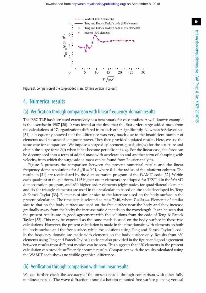
Figure 3. Comparison of the surge added mass. (Online version in colour.)

4. Numerical results

(a) Verification through comparison with linear frequency-domain resultsThe ISSC TLP has been used extensively as a benchmark for case studies. A well-known exampleis the exercise in 1987 [30]. It was found at the time that the first-order surge added mass fromthe calculations of 17 organizations differed from each other significantly. Newman & Sclavounos[31] subsequently showed that the difference was very much due to the insufficient number ofelements used because of computer power. They then provided updated results. Here, we use thesame case for comparison. We impose a surge displacement ζ1 = S1 sin(ωt) for the structure andobtain the surge force F(t) when it has become periodic at t> t0. For the linear case, the force canbe decomposed into a term of added mass with acceleration and another term of damping withvelocity, from which the surge added mass can be found from Fourier analysis.

Figure 3 presents the comparison between the present numerical results and the linearfrequency-domain solutions for S1/R = 0.01, where R is the radius of the platform column. Theresults in [31] are recalculated by the demonstration program of the WAMIT code [32]. Withineach quadrant of the platform, 1145 higher order elements are adopted for TEST14 in the WAMTdemonstration program, and 630 higher order elements (eight nodes for quadrilateral elementsand six for triangle elements) are used in the recalculation based on the code developed by Teng& Eatock Taylor [33]. Elements of similar size to the latter are used on the body surface in thepresent calculation. The time step is selected as t = T/40, where T = 2π/ω. Elements of similarsize to that on the body surface are used on the free surface near the body and they increasegradually away from the body; the increase ratio depends on the wavelength. It can be seen thatthe present results are in good agreement with the solutions from the code of Teng & EatockTaylor [33]. This may be expected as the same mesh is used on the body surface in these twocalculations. However, the present calculation is made in the time domain with elements on boththe body surface and the free surface, while the solutions using Teng and Eatock Taylor’s codein the frequency domain are made with elements on the body surface only. Results from 630elements using Teng and Eatock Taylor’s code are also provided in the figure and good agreementbetween results from different meshes can be seen. This suggests that 630 elements in the presentcalculation can provide sufficiently accurate results. Comparison with the results calculated usingthe WAMIT code shows no visible graphical difference.

(b) Verification through comparison with nonlinear resultsWe can further check the accuracy of the present results through comparison with other fullynonlinear results. The wave diffraction around a bottom-mounted free-surface piercing vertical



11


.........................................................

X

Y

–1.0 –0.5 0 0.5 1.00

0.5

1.0

(a) (b)

Figure 4. The initial meshes on the free surface and the cylinder for Mesh b: (a) free surface and (b) cylinder surface.

6.0

6.2

6.4

6.6

6.8

7.0

0 0.05 0.10 0.15 0.20 0.251.0

1.5

2.0

2.5

(a) analytical experiment Shao and Faltinsen

Ferrant present (5th, Mesh a)

present (5th, Mesh b) present (20th, Mesh b)

(b)

kA

arg

(F(1

) )x

F(1

) /rgA

R2

x

Figure5. Comparisonof thefirst-harmonic horizontal force: (a) amplitudeof the force and (b) phaseof the force. (Online versionin colour.)

circular cylinder with radius of R and water depth of d/R = 20 at wavenumber kR = 0.245 isconsidered. This is the same case which has been studied experimentally by Huseby & Grue[34] and numerically by Ferrant [21] and Shao & Faltinsen [24] using a fully nonlinear theory.

Two different meshes are used in the present calculation. Mesh a has 664 elements and 2209nodes on the full boundary, and Mesh b has 1320 and 4255, respectively. The initial meshes on thefree surface and the cylinder for Mesh b are shown in figure 4. The ratio between the radius of theouter truncated cylinder radius and R is 46 and the radial length of the damping zone is set to beone wavelength. Figures 5–8 show the results for the first-, second-, third- and fourth-harmonicforces, respectively. It can be seen from these figures that the present results from the two meshesare almost graphically identical. To check whether the fifth-order Stokes incident wave is a goodapproximation for the present case, we have run the simulation with Mesh b using the twentieth-order Stokes wave [35], and it makes hardly any visible difference to the results. Comparisonswith the experimental results of Huseby & Grue [34], and fully nonlinear numerical results ofFerrant [21] and Shao & Faltinsen [24] show that they are in fairly good agreement. There is somediscrepancy between all the numerical results and the experimental data in the second-harmonicforces. As commented by Shao & Faltinsen [24], the free second-harmonic waves which originateat the wave maker in the experiment may be the reason.



12


.........................................................

analytical experiment Shao and Faltinsen



0 0.05 0.10 0.15 0.20 0.25kA

(a)

(b)

arg

(F(2

) )x

F(2

) /rgA

R2

x

0

0.3

0.6

0.9

1.2

1

2

3

Figure 6. Comparison of the second-harmonic horizontal force: (a) amplitude of the phase and (b) phase of the force. (Onlineversion in colour.)

analytical experiment Shao and Faltinsen



0 0.05 0.10 0.15 0.20 0.25kA

(a)

(b)

arg

(F(3

) )x

F(3

) /rgA

R2

x

0

0.2

0.4

0.6

0.8

–3

–2

–1

0

1

Figure 7. Comparison of the third-harmonic horizontal force: (a) amplitude of the force and (b) phase of the force. (Onlineversion in colour.)

(c) Analysis of platformmotion near the pitch natural frequencyTo undertake the convergence study for the higher order force on the ISSC platform, we runa simulation for uncoupled pitch motion at A/R = 0.12 and ω

√R/g =ω′

n5√

R/g/3 = 1.006. Thedamping zone starts from a horizontal distance at Ddc = 15R to the centre of the space-fixedsystem and the radial length of the damping zone is set to be one linear wavelength λ= 5.7R.Two different meshes are chosen. There are 1775 elements and 11 395 nodes on the full boundaryin Mesh a, as shown in figure 9, and the number of elements and nodes of Mesh b is 3486 and



13


.........................................................

Shao and Faltinsen

Ferrant

present (5th, Mesh b)

experiment

present (5th, Mesh a)

present (20th, Mesh b)

0 0.05 0.10 0.15 0.20 0.25kA

(a)

(b)

arg

(F(4

) )x

F(4

) /rgA

R2

x

0

0.2

0.4

0.6

0.8

1

2

3

4

5

Figure 8. Comparison of the fourth-harmonic horizontal force: (a) amplitude of the force and (b) phase of the force. (Onlineversion in colour.)

X

Y

–100 0 1000

50

100

150

(a) (b)

Figure 9. The initial meshes on the free surface and the TLP for Mesh a: (a) free surface and (b) TLP surface.

Table 3. Error analysis of first three harmonic pitch amplitudes at different meshes and time steps.

Mesh a Mesh b Mesh a |fia − fib|/fib |fi t1 − fi t2 |/fi t2

( t1 = T/40) ( t1 = T/40) ( t2 = T/80) (%) (%). . . . . . . . . . . . . . . . . . . . . . . . . . . . . . . . . . . . . . . . . . . . . . . . . . . . . . . . . . . . . . . . . . . . . . . . . . . . . . . . . . . . . . . . . . . . . . . . . . . . . . . . . . . . . . . . . . . . . . . . . . . . . . . . . . . . . . . . . . . . . . . . . . . . . . . . . . . . . . . . . . . . . . . . . . . . . . . . . . . . . . . . . . . . . . . . . . . . . . . . . .

ζ(1)5 R/A 0.0002111 0.0002106 0.0002110 0.24 0.05

. . . . . . . . . . . . . . . . . . . . . . . . . . . . . . . . . . . . . . . . . . . . . . . . . . . . . . . . . . . . . . . . . . . . . . . . . . . . . . . . . . . . . . . . . . . . . . . . . . . . . . . . . . . . . . . . . . . . . . . . . . . . . . . . . . . . . . . . . . . . . . . . . . . . . . . . . . . . . . . . . . . . . . . . . . . . . . . . . . . . . . . . . . . . . . . . . . . . . . . . . .

ζ(2)5 R/A 0.00003965 0.00003936 0.00003980 0.74 0.38

. . . . . . . . . . . . . . . . . . . . . . . . . . . . . . . . . . . . . . . . . . . . . . . . . . . . . . . . . . . . . . . . . . . . . . . . . . . . . . . . . . . . . . . . . . . . . . . . . . . . . . . . . . . . . . . . . . . . . . . . . . . . . . . . . . . . . . . . . . . . . . . . . . . . . . . . . . . . . . . . . . . . . . . . . . . . . . . . . . . . . . . . . . . . . . . . . . . . . . . . . .

ζ(3)5 R/A 0.0002738 0.0002628 0.0002756 4.18 0.65

. . . . . . . . . . . . . . . . . . . . . . . . . . . . . . . . . . . . . . . . . . . . . . . . . . . . . . . . . . . . . . . . . . . . . . . . . . . . . . . . . . . . . . . . . . . . . . . . . . . . . . . . . . . . . . . . . . . . . . . . . . . . . . . . . . . . . . . . . . . . . . . . . . . . . . . . . . . . . . . . . . . . . . . . . . . . . . . . . . . . . . . . . . . . . . . . . . . . . . . . . .

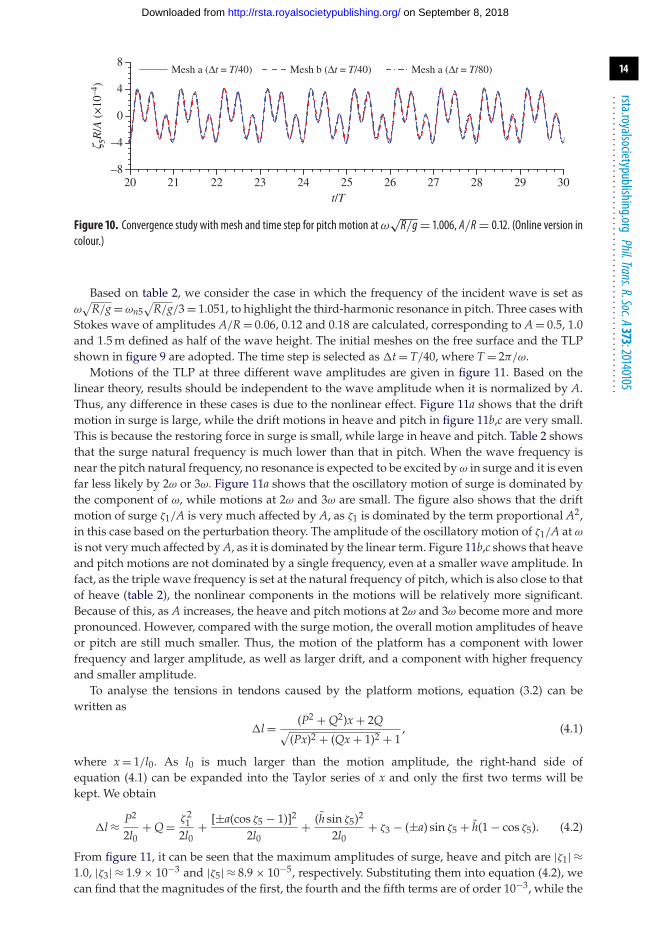
21 993. It can be seen from figure 10 that the curves from two meshes at t = T/40 and those fromMesh a at t = T/40 and for t = T/80 are graphically identical. The error analysis is presented intable 3. |fia − fib|/fib in the table denotes the relative difference of results from two different mesheswith t = T/40. |fi t1 − fi t2 |/fi t2 in the table denotes the relative difference between results fromtwo different time steps with Mesh a. They are less than 5%. This shows that the result with Mesha and time-interval t = T/40 is sufficiently accurate for these results.



14


.........................................................

20 21 22 23 24 25 26 27 28 29 30–8

–4

0

4

8

z 5R/A

(×

10–4

)

t/T

Mesh a (Dt = T/40) Mesh a (Dt = T/80)Mesh b (Dt = T/40)

Figure 10. Convergence study with mesh and time step for pitch motion atω√R/g= 1.006, A/R= 0.12. (Online version in

colour.)

Based on table 2, we consider the case in which the frequency of the incident wave is set asω

√R/g =ωn5

√R/g/3 = 1.051, to highlight the third-harmonic resonance in pitch. Three cases with

Stokes wave of amplitudes A/R = 0.06, 0.12 and 0.18 are calculated, corresponding to A = 0.5, 1.0and 1.5 m defined as half of the wave height. The initial meshes on the free surface and the TLPshown in figure 9 are adopted. The time step is selected as t = T/40, where T = 2π/ω.

Motions of the TLP at three different wave amplitudes are given in figure 11. Based on thelinear theory, results should be independent to the wave amplitude when it is normalized by A.Thus, any difference in these cases is due to the nonlinear effect. Figure 11a shows that the driftmotion in surge is large, while the drift motions in heave and pitch in figure 11b,c are very small.This is because the restoring force in surge is small, while large in heave and pitch. Table 2 showsthat the surge natural frequency is much lower than that in pitch. When the wave frequency isnear the pitch natural frequency, no resonance is expected to be excited by ω in surge and it is evenfar less likely by 2ω or 3ω. Figure 11a shows that the oscillatory motion of surge is dominated bythe component of ω, while motions at 2ω and 3ω are small. The figure also shows that the driftmotion of surge ζ1/A is very much affected by A, as ζ1 is dominated by the term proportional A2,in this case based on the perturbation theory. The amplitude of the oscillatory motion of ζ1/A at ωis not very much affected by A, as it is dominated by the linear term. Figure 11b,c shows that heaveand pitch motions are not dominated by a single frequency, even at a smaller wave amplitude. Infact, as the triple wave frequency is set at the natural frequency of pitch, which is also close to thatof heave (table 2), the nonlinear components in the motions will be relatively more significant.Because of this, as A increases, the heave and pitch motions at 2ω and 3ω become more and morepronounced. However, compared with the surge motion, the overall motion amplitudes of heaveor pitch are still much smaller. Thus, the motion of the platform has a component with lowerfrequency and larger amplitude, as well as larger drift, and a component with higher frequencyand smaller amplitude.

To analyse the tensions in tendons caused by the platform motions, equation (3.2) can bewritten as

l = (P2 + Q2)x + 2Q√(Px)2 + (Qx + 1)2 + 1

, (4.1)

where x = 1/l0. As l0 is much larger than the motion amplitude, the right-hand side ofequation (4.1) can be expanded into the Taylor series of x and only the first two terms will bekept. We obtain

l ≈ P2

2l0+ Q = ζ 2

12l0

+ [±a(cos ζ5 − 1)]2

2l0+ (h̄ sin ζ5)2

2l0+ ζ3 − (±a) sin ζ5 + h̄(1 − cos ζ5). (4.2)

From figure 11, it can be seen that the maximum amplitudes of surge, heave and pitch are |ζ1| ≈1.0, |ζ3| ≈ 1.9 × 10−3 and |ζ5| ≈ 8.9 × 10−5, respectively. Substituting them into equation (4.2), wecan find that the magnitudes of the first, the fourth and the fifth terms are of order 10−3, while the



15


.........................................................

–0.2

0.2

0.6

1.0

1.4(a)

(b)

(c)–3

–2

–1

0

1

0 5 10 15 20 25 35 36 37 38 39 40–6

–3

0

3

6

z 1/A

z 3/A

(×

10–3

)z 5R

/A (

×10

–4)

t/T

A/R = 0.06 A/R = 0.18A/R = 0.12

Figure 11. Motions of the TLP in Stokes wave with ω√R/g= 1.051 at different wave amplitudes: (a) surge, (b) heave and

(c) pitch. (Online version in colour.)

remaining terms are of order 10−7. As a result, equation (4.2) becomes

l ≈ ζ 21

2l0+ ζ3 − (±a)ζ5. (4.3)

The three terms above correspond to the contributions from surge, heave and pitch, respectively,and the tether tension contributions can be denoted as Fc1 = kζ 2

1 /2l0, Fc2 = kζ3 and Fc3 = kaζ5.Equation (4.3) shows that l is proportional to heave and pitch motions linearly. Thus, their

individual contributions to the tensions can be obtained by multiplying the results in figure 11b,cby k, respectively. The dominant term from surge in this particular example is of second order.It has been seen in figure 11a that the surge is dominated by the mean drift and the first-orderoscillatory motions. Thus, it will contribute to the tensions in tendons in terms of a steady force,and oscillatory forces at the wave frequency and the double frequency. Equation (4.3) also showsthat the surge and heave will have the same effect on tendons one and two. The effect of pitchhas the opposite phase in terms of sign. To show the behaviour of the tensions of the tendonsat the higher frequency resonance, figure 12a,b provides the tensions in tendons one and two,respectively, excluding T0, together with individual tension components in figure 13. It can beseen from figure 13 that the heave motion leads to a steady downward force. This is partlycancelled by the steady upward force caused by the surge. Thus, the mean force in the tendonsshown in figure 12a,b is much smaller. The oscillatory components at single, double and triplefrequencies at large wave amplitude are obvious in both figure 12a,b. However, due to differentsigns before the component due to the pitch in equation (4.3), the triple frequency component



16


.........................................................

–1.0

–0.5

0

0.5

1.0

–1.0

–0.5

0

0.5

1.0(b)

0 5 10 15 20 25 35 36 37 38 39 40t/T

(a)

(Fca

ble1

–T0)

/rgA

R2

(Fca

ble2

–T0)

/rgA

R2

A/R = 0.06 A/R = 0.18A/R = 0.12

Figure 12. Tensions of tendons one and two withω√R/g= 1.051 at different wave amplitudes: (a) one and (b) two. (Online

version in colour.)

30 31 32 33 34 35 36 37 38 39 40–1.0

–0.5

0

0.5

1.0 Fc1 Fc2 Fc3

F ci/r

gAR

2

t/T

Figure 13. Tension components due to the different motions atω√R/g= 1.051, A/R= 0.18. (Online version in colour.)

has opposite phase in figure 12a,b, as the pitch motion is at near resonance excited by the triplefrequency component in the wave. We note that the steady drift motion of surge is much largerthan the oscillatory component. This leads to the observation that the oscillatory component ofFc1 = kζ 2

1 /2l0 is dominated by the first-harmonic component and the second one is hardly visiblein figure 13.

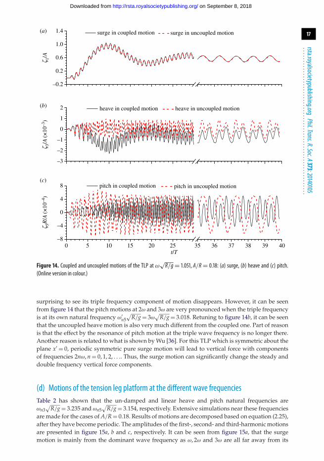
To show the coupling effects, results of coupled motion and uncoupled motion in each modeare compared, where the latter means that only a single degree of motion is allowed. Thecomparison in figure 14a at ω

√R/g = 1.051 and A/R = 0.18 shows that there is little difference

between coupled and uncoupled surge motions. This means that the surge is hardly affectedby the heave and pitch. This is expected as their motions are very small. Figure 14c shows thatthe uncoupled pitch motion is significantly different from the coupled one. In particular, thetriple frequency component becomes far less obvious. The main reason for this is the changeof the natural frequency. As discussed in §3, the coupled pitch natural frequency is ωn5

√R/g =

3.154 which is different from the uncoupled pitch natural frequency ω′n5

√R/g = 3.018. Thus the

uncoupled motion in figure 14c is no longer at triple frequency resonance and it is therefore not



17


.........................................................

–0.2

0.2

0.6

1.0

surge in coupled motion surge in uncoupled motion

heave in coupled motion heave in uncoupled motion

pitch in coupled motion pitch in uncoupled motion

1.4(a)

(b)

(c)

–3

–2

–1

0

1

2

0 5 10 15 20 25 35 36 37 38 39 40–8

–4

0

4

8

z 1/A

z 3/A

(×10

–3)

z 5R/A

(×10

–4)

t/T

Figure 14. Coupled and uncoupled motions of the TLP at ω√R/g= 1.051, A/R= 0.18: (a) surge, (b) heave and (c) pitch.

(Online version in colour.)

surprising to see its triple frequency component of motion disappears. However, it can be seenfrom figure 14 that the pitch motions at 2ω and 3ω are very pronounced when the triple frequencyis at its own natural frequency ω′

n5√

R/g = 3ω√

R/g = 3.018. Retuning to figure 14b, it can be seenthat the uncoupled heave motion is also very much different from the coupled one. Part of reasonis that the effect by the resonance of pitch motion at the triple wave frequency is no longer there.Another reason is related to what is shown by Wu [36]. For this TLP which is symmetric about theplane x′ = 0, periodic symmetric pure surge motion will lead to vertical force with componentsof frequencies 2nω, n = 0, 1, 2, . . .. Thus, the surge motion can significantly change the steady anddouble frequency vertical force components.

(d) Motions of the tension leg platform at the different wave frequenciesTable 2 has shown that the un-damped and linear heave and pitch natural frequencies areωn3

√R/g = 3.235 and ωn5

√R/g = 3.154, respectively. Extensive simulations near these frequencies

are made for the cases of A/R = 0.18. Results of motions are decomposed based on equation (2.25),after they have become periodic. The amplitudes of the first-, second- and third-harmonic motionsare presented in figure 15a, b and c, respectively. It can be seen from figure 15a, that the surgemotion is mainly from the dominant wave frequency as ω, 2ω and 3ω are all far away from its



18


.........................................................

1.00 1.05 1.10 1.150

0.03

0.06

0.09

0.12(a) (b)

0

0.2

0.4

0.6

0.8

1.0

0

1

2

3

4

5

z 1(m) /A

z 3(m) /A

(×10

–3)

z 5(m) R

/A(×

10–4

)

w R/g1.00 1.05 1.10 1.15

w R/g

1.00 1.05 1.10 1.15

w R/g

m = 1 m = 2 m = 3

(c)

Figure 15. Amplitudes of the first-, second- and third-harmonic motions versus wave frequency at A/R= 0.18: (a) surge,(b) heave and (c) pitch. (Online version in colour.)

1.00 1.05 1.10 1.15

0.2

0.4

0.6

00

0.2

0.4

0.6(b)

m = 1 m = 2 m = 3(a)

(Fca

ble1

–T0)

(m) /r

gAR

2

(Fca

ble2

–T0)

(m) /r

gAR

2

w R/g

1.00 1.05 1.10 1.15

w R/g

Figure 16. Amplitudes of the first- and second-harmonic tensions of tendons one and two versus wave frequency atA/R= 0.18: (a) one and (b) two. (Online version in colour.)

natural frequency. It is most interesting to see from figure 15b,c that the maxima of the third-harmonic heave and pitch motions occur at ω

√R/g ≈ 1.081 and ω

√R/g ≈ 1.055, respectively,

which implies the natural frequencies at 3.243 and 3.165, respectively. They are slightly differentfrom the un-damped linear results in table 2. Figure 15b shows that the away from the resonantregion the third-harmonic heave motion amplitude is significantly reduced and it is smaller thanthe first- and second-harmonic ones. Similar results for the pitch can be seen in figure 15c. All theseshow the importance of avoiding the triple wave frequency getting near the natural frequency ofheave or pitch.



19


.........................................................

The amplitudes of the first-, second- and third-harmonic tensions of tendons one and twoare shown in figure 16a,b, respectively. It can be seen from the figures that the variations of thefirst- and second-harmonic tensions of the tendons are smooth, while there are several peaks andtroughs in the third-harmonic ones. From equation (4.3), it can be seen that the third-harmonictensions of the tendons are due to the combined effect of the third-harmonic heave and pitchmotions, as the contribution of the third-harmonic surge motion is negligible. From figure 15b,c,we can see that the natural pitch and heave frequencies are 3 × ω

√R/g ≈ 3 × 1.055 = 3.165 and

3 × ω√

R/g ≈ 3 × 1.081 = 3.243, respectively, which may be slightly different from the undamped

natural frequencies in table 2. At ω√

R/g ≈ 1.055, the maximum amplitude of kaζ (3)5 /ρgAR2 is

about 0.5, while that of kζ (3)3 /ρgAR2 is about 0.05. Thus the contribution to the tensions of

the tendons at this frequency mainly comes from the pitch motion. As a result, the third-harmonic tensions of tendons one and two both show a maximum around ω

√R/g ≈ 1.055. At

ω√

R/g ≈ 1.081, which is related to the heave resonance, the maximum amplitude of kζ (3)3 /ρgAR2

is about 0.19, while that of kaζ (3)5 /ρgAR2 is about 0.14. Thus, the contributions to the tensions

of the tendons from the heave and pitch motions are comparable. This means that the peak inheave does not automatically lead to a peak in the tensions. In fact, due to the combined effectof heave and pitch, the second local peak of the tension occurs at ω

√R/g ≈ 1.078 for tendon

one and ω√

R/g ≈ 1.085 for tendon two, slightly away from the heave resonant frequency atω

√R/g ≈ 1.081. We may also note from figure 16b that there is a local trough at ω

√R/g ≈ 1.074

for tendon two. This is because the amplitudes of kζ (3)3 /ρgAR2 and kaζ (3)

5 /ρgAR2 are comparablebut their phases are almost opposite one another for tendon two, which leads to the partialcancellation in the tension.

5. ConclusionA higher order BEM has been used to investigate the resonance of a floating TLP generatedby the third-harmonic force in nonlinear regular waves. The comparison of the surge addedmass at small amplitude motion, together with the comparison for the higher order forceon a vertical cylinder suggest that the present model provides accurate results. The resonantbehaviour generated by the third-order force at the triple wave frequency is well captured andinvestigated. It becomes more pronounced when the incoming wave amplitude increases as thetriple frequency force is dominated by the term of the cube of the wave amplitude. When thetriple frequency of the incoming wave is close to the higher natural frequency of the platform,its surge motion with its lower natural frequency will have large amplitude at wave frequency,as well as a large drift. Its heave and pitch motions with higher natural frequencies will bedominated by responses at the triple wave frequency, even though the amplitudes may be muchsmaller than that of the surge. The comparison between the results from the coupled motionand the uncoupled motion around this wave frequency shows that the surge motion is hardlyaffected by heave and pitch motions, while heave and pitch motions, as well as the pitch naturalfrequency, are very much affected by the surge. Extensive simulations have been made whenthe triple wave frequency is near the natural frequencies of the heave and pitch. It is noted thatthese natural frequencies are affected by the wave amplitude. The third-harmonic heave and pitchmotion amplitudes are significantly reduced when the triple wave frequency is away from theircorresponding natural frequencies. The effect of the heave and pitch on the tensions of the tendonsis dominated by their linear terms, while the effect of the surge is dominated by the second-orderterm. The different phases of these motions can reinforce the tensions in some tendons whilecause partial cancellation in others. In the design and operation of this type of offshore platform,it is important to avoid the high-frequency resonance and to adjust the phase difference of eachmotion, or to control their adverse effects.

Acknowledgements. The authors have greatly benefited from the most inspiring and helpful discussions withProfs R. Eatock Taylor and J. N. Newman. The valuable contribution from Prof. B. Teng and Dr Y. L. Shao isalso gratefully acknowledged.



20


.........................................................

Funding statement. The authors gratefully acknowledge financial support from the Lloyd’s Register Foundation(LRF) through the joint centre involving University College London, Shanghai Jiaotong University andHarbin Engineering University. The LRF helps to protect life and property by supporting engineering-related education, public engagement and the application of research. This work is also supported by theNational Natural Science Foundation of China (51409066), and the China Postdoctoral Science Foundation(2014M550183).

References1. Mercier JA. 1982 Evolution of tension leg platform technology. In Proc. of 3rd Int. Conf. on the

Behaviour of Offshore Structures, Boston, MA, 2–5 August 1982. Cambridge, MA: MIT.2. Tromans P, Swan C, Masterton S. 2006 Nonlinear potential flow forcing: the ringing of concrete

gravity based structures. Health and Safety Executive Report, UK.3. Report from the Ringing Joint Industry Project. 1993 Higher order wave load effects on large

volume structures. Task2: interpretation of existing measurements - Project Memo. MT51-F93–0100.Marintek Sintef Group, Norway.

4. Petrauskas C, Liu SV. 1987 Springing force response of a tension leg platform. In Offshore TechnologyConf., Houston, TX, 27–30 April 1987, pp. 333–341. Society of Petroleum Engineers.

5. Scolan YM, Le Boulluec M, Chen XB, Deleuil G, Ferrant P, Malenica S, Molin B. 1997 Someresults from numerical and experimental investigations on the high frequency responses of offshorestructures. In Proc. of BOSS’97, Delft, The Netherlands, 7–10 July 1997, pp. 127–142. ElsevierScience & Technology.

6. Chaplin JR, Rainey RCT, Yemm RW. 1997 Ringing of a vertical cylinder in waves. J. Fluid Mech.350, 119–147. (doi:10.1017/S002211209700699X)

7. Stansberg CT, Huse E, Krogstad JR, Lehn E. 1995 Experimental study of non-linear loads onvertical cylinders in steep random waves. In Proc. 5th Int. Offshore and Polar Eng. Conf. Int. Societyof Offshore and Polar Engineers, The Hague, Netherlands, 11–16 June, pp. 75–82. InternationalSociety of Offshore and Polar Engineers.

8. Kim CH, Zhao CT, Zou J, Xu Y. 1997 Springing and ringing due to laboratory-generatedasymmetric waves. Int. J. Offshore Polar. Eng. 7, 30–35.

9. Zou J, Xu Y, Kim CH. 1998 Ringing of ISSC TLP due to laboratory storm seas. Int. J. OffshorePolar. Eng. 8, 81–89.

10. Wang ZM, Kim CH. 2001 Nonlinear response of ISSC TLP in high and steep random waves.In Proc. 11th Int. Offshore and Polar Eng. Conf., Stavanger, Norway, 17–22 June, pp. 440–446.Cupertino, CA: International Society of Offshore and Polar Engineers.

11. Faltinsen ON, Newman JN, Vinje T. 1995 Nonlinear wave loads on a slender vertical cylinder.J. Fluid Mech. 289, 179–198. (doi:10.1017/S0022112095001297)

12. Malenica S, Molin B. 1995 Third-harmonic wave diffraction by a vertical cylinder. J. Fluid Mech.302, 203–229. (doi:10.1017/S0022112095004071)

13. Teng B, Kato S. 2002 Third order wave force on axisymmetric bodies. Ocean Eng. 29, 815–843.(doi:10.1016/S0029-8018(01)00047-6)

14. Wu GX, Hu ZZ. 2004 Simulation of nonlinear interactions between waves and floatingbodies through a finite-element-based numerical tank. Proc. R. Soc. Lond. A 460, 2797–2817.(doi:10.1098/rspa.2004.1302)

15. Wang CZ, Wu GX, Drake KR. 2007 Interactions between fully nonlinear water waves andnon-wall-sided 3D structures. Ocean Eng. 34, 1182–1196. (doi:10.1016/j.oceaneng.2006.07.005)

16. Yan S, Ma QW. 2009 QALE-FEM numerical modelling of non-linear interaction between3D moored floating bodies and steep waves. Int. J. Numer. Methods Eng. 78, 713–756.(doi:10.1002/nme.2505)

17. Liu YM, Xue M, Yue DKP. 2001 Computations of fully nonlinear three dimensional wave–wave and wave–body interactions. Part 2: nonlinear waves and forces on a body. J. Fluid Mech.438, 41–46.

18. Bai W, Eatock Taylor R. 2009 Fully nonlinear simulation of wave interaction with fixed andfloating flares structures. Ocean Eng. 36, 223–236. (doi:10.1016/j.oceaneng.2008.11.003)

19. Yan HM, Liu YM. 2011 An efficient high-order boundary element method for nonlinearwave-wave and wave-body interactions. J. Comput. Phys. 230, 402–424. (doi:10.1016/j.jcp.2010.09.029)

20. Ferrant P. 1997 Simulation of strongly nonlinear wave generation and wave-body interactionsusing a 3-D MEL model. In Proc. 21st Symp. Naval Hydro, Trondheim, Norway, pp. 93–109.


http://dx.doi.org/doi:10.1017/S002211209700699X

http://dx.doi.org/doi:10.1017/S0022112095001297


http://dx.doi.org/doi:10.1016/S0029-8018(01)00047-6

http://dx.doi.org/doi:10.1098/rspa.2004.1302

http://dx.doi.org/doi:10.1016/j.oceaneng.2006.07.005

http://dx.doi.org/doi:10.1002/nme.2505

http://dx.doi.org/doi:10.1016/j.oceaneng.2008.11.003

http://dx.doi.org/doi:10.1016/j.jcp.2010.09.029



21


.........................................................

21. Ferrant P. 1999 Fully nonlinear interactions of long-crested wave packets with a threedimensional body. In Proc. 22nd Symp., Washington, DC, 9–14 August 1998, pp. 403–415.Washington, DC: National Academies Press.

22. Ferrant P, Le Touzé D, Pelletier K. 2003 Nonlinear time-domain models for irregularwave diffraction about offshore structures. Int. J. Numer. Meth. Fluids 43, 1257–1277.(doi:10.1002/fld.506)

23. Ducrozet G, Engsig-Karup AP, Bingham HR, Ferrant P. 2014 A non-linear wavedecomposition model for efficient wave-structure interaction. Part A: formulation, validationsand analysis. J. Comput. Phys. 257, 863–883.

24. Shao YL, Faltinsen OM. 2014 A harmonic polynomial cell (HPC) method for 3D Laplaceequation with application in marine hydrodynamics. J. Comput. Phys. 274, 312–332.(doi:10.1016/j.jcp.2014.06.021)

25. Zhou BZ, Wu GX, Teng B. 2015 Fully nonlinear wave interaction with freely floating non-wall-sided structures. Eng. Anal. Bound. Elem. 50, 117–132. (doi:10.1016/j.enganabound.2014.08.003)

26. Thornton ST, Marion JB. 2003 Classical dynamics of particles and systems, 5th edn, pp. 440–447.Belmont, CA: Thomson Learning Academic Resource Center.

27. Fenton JD. 1985 A fifth order Stokes theory for steady waves. J. Waterway Port Coastal OceanEng. 111, 216–234. (doi:10.1061/(ASCE)0733-950X(1985)111:2(216))

28. Fluent Inc. 2004 Gambit 2.4 tutorial guide. Lebanon, NH: FLUENT User Service. Fluent Inc.29. Wu GX, Eatock Taylor R. 2003 The coupled finite element and boundary element

analysis of nonlinear interactions between waves and bodies. Ocean Eng. 30, 387–400.(doi:10.1016/S0029-8018(02)00037-9)

30. Eatock Taylor R, Jefferys ER. 1986 Variability of hydrodynamic load predictions for a tensionleg platform. Ocean Eng. 13, 449–490. (doi:10.1016/0029-8018(86)90033-8)

31. Newman JN, Sclavounos PD. 1988 The computation of wave loads on large offshorestructures. In Proc. of BOSS’88, Trondheim, Norway, June, pp. 605–622. Trondheim, Norway:Tapir publishers.

32. Wamit Inc. 2013 Wamit user manual v. 7.0. Chestnut Hill, MA: Wamit Inc.33. Teng B, Eatock Taylor R. 1987 New higher-order boundary elements methods for wave

diffraction/radiation. Appl. Ocean Res. 9, 19–30. (doi:10.1016/0141-1187(87)90028-9)34. Huseby M, Grue J. 2000 An experimental investigation of higher-harmonic wave forces on a

vertical cylinder. J. Fluid Mech. 414, 75–103. (doi:10.1017/S0022112000008533)35. Rienecker MM, Fenton JD. 1981 A Fourier approximation method for steady water waves.

J. Fluid Mech. 104, 119–137. (doi:10.1017/S0022112081002851)36. Wu GX. 2000 A note on non-linear hydrodynamic forces on a floating body. Appl. Ocean Res.

22, 315–316. (doi:10.1016/S0141-1187(00)00016-X)


http://dx.doi.org/doi:10.1002/fld.506


http://dx.doi.org/doi:10.1016/j.enganabound.2014.08.003

http://dx.doi.org/doi:10.1061/(ASCE)0733-950X(1985)111:2(216)

http://dx.doi.org/doi:10.1016/S0029-8018(02)00037-9

http://dx.doi.org/doi:10.1016/0029-8018(86)90033-8

http://dx.doi.org/doi:10.1016/0141-1187(87)90028-9



http://dx.doi.org/doi:10.1016/S0141-1187(00)00016-X


Resonanceofatension legplatformexitedby third...

Documents

Transcript of Resonanceofatension legplatformexitedby third...