An applied mathematics perspective on stochastic modelling...

on August 30, 2018http://rsta.royalsocietypublishing.org/Downloaded from

An applied mathematics perspectiveon stochastic modelling for climate

BY ANDREW J. MAJDA1,*, CHRISTIAN FRANZKE

2

AND BOUALEM KHOUIDER3

1Department of Mathematics and Center for Atmosphere-Ocean Science,Courant Institute of Mathematical Sciences, New York University,

New York, 10012 NY, USA2British Antarctic Survey, Natural Environment Research Council,

Cambridge CB3 0ET, UK3Department of Mathematics and Statistics, University of Victoria,

Victoria, BC, Canada V8W 3P4

Systematic strategies from applied mathematics for stochastic modelling in climate arereviewed here. One of the topics discussed is the stochastic modelling of mid-latitudelow-frequency variability through a few teleconnection patterns, including the centralrole and physical mechanisms responsible for multiplicative noise. A new low-dimensional stochastic model is developed here, which mimics key features ofatmospheric general circulation models, to test the fidelity of stochastic mode reductionprocedures. The second topic discussed here is the systematic design of stochastic latticemodels to capture irregular and highly intermittent features that are not resolved by adeterministic parametrization. A recent applied mathematics design principle forstochastic column modelling with intermittency is illustrated in an idealized settingfor deep tropical convection; the practical effect of this stochastic model in both slowingdown convectively coupled waves and increasing their fluctuations is presented here.

Keywords: low-frequency variability; tropical convection; multiplicative noise;intermittency

On

*A

1. Introduction

Stochastic modelling for climate is important for understanding the intrinsicvariability of dominant low-frequency teleconnection patterns in climate, toprovide cheap low-dimensional computational models for the coupled atmosphere–ocean system and to reduce model error in standard deterministic computer modelsfor extended-range prediction through appropriate stochastic noise (Palmer 2001).

The present contribution is a research-expository paper on systematic strategiesfor stochastic climate modelling from the perspective of modern appliedmathematics. In the modern applied mathematics, ‘modus operandi’ rigorousmathematical analysis, qualitative, asymptotic and numerical modelling are all

Phil. Trans. R. Soc. A (2008) 366, 2429–2455

doi:10.1098/rsta.2008.0012

Published online 29 April 2008

e contribution of 12 to a Theme Issue ‘Stochastic physics and climate modelling’.

uthor for correspondence ([email protected]).

2429 This journal is q 2008 The Royal Society

http://rsta.royalsocietypublishing.org/

A. J. Majda et al.2430


blended together in a multidisciplinary fashion to provide systematic guidelines toaddress real-world problems (Majda 2000). For stochastic modelling in climate, themodern applied mathematics tool kit includes stochastic differential equations anddiscontinuous Markov jump processes (Gardiner 1985), systematic asymptoticreduction techniques, nonlinear dynamical systems theory and ideas from bothstatistical physics (Majda & Wang 2006) and mathematical statistics (Kravtsovet al. 2005; Majda et al. 2006a); mathematical rigour provides unambiguousguidelines in idealized models. Another facet of the modern applied mathematicsphilosophy is the development of qualitative models that represent a Platonic idealfor central issues simultaneously in diverse scientific disciplines such as materialscience, biomolecular dynamics and climate science.

In §2, we illustrate and apply this modern applied mathematics philosophy tostochastic modelling of the low-frequency variability of the atmosphere. Thesystematic mathematical theory (Majda et al. 1999, 2001, 2002, 2003, 2006b;collectively referred to as MTV hereafter; Franzke et al. 2005; Franzke & Majda2006) for these problems is briefly reviewed including the central role andphysical mechanisms responsible for multiplicative noise in the low-frequencydynamics. In this context, the Platonic ideal from applied mathematics is thetruncated Burgers–Hopf model (Majda & Timofeyev 2000). A new simplifiedlow-dimensional stochastic model that reproduces key features of atmosphericgeneral circulation models (GCMs) is used there to test the fidelity of stochasticmode reduction techniques. A recent diagnostic statistical test with firmmathematical underpinning for understanding and interpreting the dynamicalsources of the small departures from Gaussianity in low-frequency variables(Franzke et al. 2007) is also developed there.

While §2 deals with applied mathematical modelling through stochasticdifferential equations and §3 is devoted to the systematic development ofstochastic lattice models to capture unresolved features that are highlyintermittent in space and time such as deep convective clouds, cloud cover insubtropical boundary layers, sub-mesoscale eddies in the ocean and mesoscale seaice cover. Here the mathematical tools involve a family of discontinuous Markovjump processes with multi-scale behaviour in space–time called stochastic spin-flip models. The key mathematical development involves systematic strategies tocoarse grain such stochastic spin-flip models to achieve computational efficiencywhile retaining crucial features of the microscale interactions (Katsoulakis &Vlachos 2003; Katsoulakis et al. 2003a,b). The use of such stochastic latticemodels to parametrize key features of tropical convection is briefly reviewed(Majda & Khouider 2002; Khouider et al. 2003). For the coupling of continuummodels like a GCM to a stochastic lattice model as well as in many diverseapplications, an applied mathematics Platonic ideal model has recently beenintroduced and analysed by Katsoulakis et al. (2004, 2005, 2006, 2007; hereafterKMS). This model consists of a system of ordinary differential equations (ODEs)for continuum variables X,

dX

dtZFðX; �sÞ; ð1:1Þ

two-way coupled to a stochastic spin-flip model written abstractly here as

d

dtEf ðsÞZ ELf ðsÞ; ð1:2Þ

Phil. Trans. R. Soc. A (2008)


2431An applied mathematics perspective


where �s denotes the spatial coverage; L is the generator; f is a test function; and E

denotes the expected value. This idealized class of models has been used tosystematically analyse the effects of various coarse-graining procedures onprocesses with intermittency, large-scale bifurcations and microscale phasetransitions (KMS 2004, 2005, 2006, 2007). A concrete example for tropicalconvection in climate is given in §3. A new application of these stochastic latticemodels to capture intermittent features and improve the fidelity of deterministicparametrizations of convection with clear deficiencies is developed in §3. First,the systematic design principles for (1.1) and (1.2) (KMS 2006, 2007) are used tocalibrate a stochastic column model for tropical convection with intermittencyand then the new results are presented on the practical effect of slowing downconvectively coupled waves and increasing their fluctuations through thestochastic lattice models.

2. Systematic low-dimensional stochastic mode reductionand atmospheric low-frequency variability

A remarkable fact of Northern Hemisphere low-frequency variability is that itcan be efficiently described by only a few teleconnection patterns that explainmost of the total variance (e.g. Wallace & Gutzler 1981). These fewteleconnection patterns not only exert a strong influence on regional climateand weather but are also related to climate change (Hurrell 1995). Theseproperties of teleconnection patterns make them an attractive choice as basisfunctions for climate models with a highly reduced number of d.f. Thedevelopment of such reduced climate models involves the solution of twomajor issues: (i) how to properly account for the unresolved modes that are alsoknown as the closure problem, and (ii) how to define a small set of basis functionsthat optimally represent the dynamics of the major teleconnection patterns. Thissection addresses primarily the first issue and presents a rigorous strategy of howto systematically account for the unresolved d.f.

The simplest approach to derive highly truncated models of teleconnectionpatterns is to empirically fit simple stochastic models (e.g. autoregressive modelsand fractionally differenced models) to individual scalar teleconnection indices(Feldstein 2000; Stephenson et al. 2000; Percival et al. 2001). Statistical testsusually cannot distinguish if short- or long-memory models provide the better fit.A more complex approach, which also tries to capture deterministic interactionsbetween different teleconnection patterns, is to linearize the equations of motionaround a climatological mean state. Such models can be determined empiricallyfrom data or by using the linearized equations of motion. These models can beforced either by a random forcing (Branstator 1990; Newman et al. 1997;Whitaker & Sardeshmukh 1998; Zhang & Held 1999) or by an external forcingrepresenting tropical heating (Branstator & Haupt 1998). To ensure stability ofthese linear models, damping is added according to various ad hoc principles.There is a recent survey of such modelling strategies (Delsole 2004).

A more powerful method is to empirically fit nonlinear stochastic models withpossibly multiplicative (state dependent) noise by using the Fokker–Planckequation (Gardiner 1985; Sura 2003; Berner 2005). To reliably estimate the driftand diffusion coefficients in the Fokker–Planck equation is a subtle inverse





problem that requires very long time series, and is further complicated by theneed to retain the leading-order eigenvalue structure of the Fokker–Planckoperator in order to keep the autocorrelation time scales of the original model(Crommelin & Vanden-Eijnden 2006); the fitting procedure in most of the recentwork is the most attractive current regression strategy for low-frequencybehaviour. Recently, Kravtsov et al. (2005) have developed a simplified nonlinearregression strategy that produces very good results for a three-layer quasi-geostrophic model with a realistic climate. However, order 2000 regressioncoefficients need to be fitted in a model with order 1000 state variables to achievethese results. Some inherent limitations of this approach in describing the correctphysics are discussed briefly below in a simplified model.

All the work presented above derives reduced models by regression fitting ofthe resolved modes. Another approach is to take advantage of the basis functionproperty of teleconnection patterns. Schubert (1985), Selten (1995), Achatz &Branstator (1999) and Achatz & Opsteegh (2003a,b) developed low-order modelswith empirical orthogonal functions (EOFs) as basis functions. Truncated EOFmodels experience climate drift due to the neglected interactions with theunresolved modes. Selten (1995) and Achatz & Branstator (1999) parametrizethese neglected interactions by a linear damping, whose strength is determinedempirically. A possibly more powerful tool to represent the dynamics of a systemis principal interaction patterns (PIPs; Hasselmann 1988; Kwasniok 1996, 2004).The calculation of PIPs takes into account the dynamics of the model for whichone tries to find an optimal basis and also often involves ad hoc closure throughlinear damping and an ansatz for nonlinear interactions. Crommelin & Majda(2004) compare different optimal bases. They find that the models based on PIPsare superior to models based on EOFs. On the other hand, they also point outthat the determination of PIPs can show sensitivities regarding the calculationprocedure, at least for some low-order atmospheric dynamical systems withregime transitions. Furthermore, PIPs have two more disadvantages: (i) muchhigher computational cost than EOFs, and (ii) one needs not only data as forEOFs but also the dynamical equations to calculate PIPs. These features canmake PIPs possibly a less attractive basis.

Majda et al. (1999, 2001, 2002, 2003, 2005, 2006a,b) provide a systematic frame-work for how to account for the effect of the fast d.f. on the slow modes incombination with using the dominant teleconnection patterns as basis functions. Incontrast to the empirical fitting procedures applied in the studies discussed above,the stochastic mode reduction strategy put forward in MTV predicts the functionalform of all deterministic and stochastic correction terms and provides a minimalregression fitting procedure of only the fast modes (Franzke et al. 2005; Franzke &Majda 2006). In general, only an estimate for the variance and eddy turnover timefor each fast mode is needed. It has been applied and tested on a wide variety ofsimplified models and examples.

(a ) Overview of the MTV strategy

We illustrate the ideas for stochastic climate modelling by considering thefollowing prototype equation for geophysical flow:

vu

vtZFCLuCBðu; uÞ: ð2:1Þ





The above functional form (2.1) is typical of dry dynamical cores of climatemodels, but the MTV strategy is easily extended to include non-quadraticnonlinearities such as associated with boundary fluxes and moist processes. Instochastic climate modelling, the variable u is decomposed into an orthogonaldecomposition through the variables ~u and u0, which are characterized bystrongly differing time scales (MTV 1999; Majda et al. 2005). The variable ~udenotes a slow low-frequency mode (also referred to as climate mode) of thesystem, which evolves slowly in time compared with the u0 variables (alsoreferred to as fast mode). By decomposing uZ ~uCu 0 in terms of some optimalenergy norm basis, we can write them as

u ZXNiZ1

aiei ZXRiZ1

aiei CXN

jZRC1

bjej ; ð2:2Þ

with ~uZPR

iZ1 aiei and u 0ZPN

jZRC1 bjej , where R is the number of climate

modes; ai denotes the expansion coefficients; and ai and bj are the expansioncoefficients of the slow (fast) modes. The use of the energy norm ensures theconservation of energy by the nonlinear operator (Selten 1995). By properlyprojecting the energy norm basis, derived from the geophysical model, ontoequation (2.1), we get two sets of equations for slow ai and fast bi modes

_aiðt ÞZ 3Hai C

Xj

Laaij ajðt ÞC

1

3

Xj

Labij bjðt ÞC

Xjk

B aaaijk ajðt Þakðt Þ

C2

3

Xjk

B aabijk ajðt Þbkðt ÞC

1

3

Xjk

B abbijk bjðt Þbkðt Þ; ð2:3Þ

_biðt ÞZ 3Hbi C

1

3

Xj

Lbaij ajðt ÞC

1

3

Xj

Lbbij bjðt ÞC

1

3

Xjk

B baaijk ajðt Þakðt Þ

C2

3

Xjk

B babijk ajðt Þbkðt ÞC

1

32

Xjk

B bbbijk bjðt Þbkðt Þ; ð2:4Þ

where the nonlinear operators have been symmetrized, that is, BijkZBikj in (2.3)and (2.4). The upper indices a and b indicate the respective subsets of the fulloperators in (2.1). Here 3 is a small positive parameter that controls theseparation of time scale between the slow and fast modes and measures the ratioof the correlation time of the slowest non-climate mode u0 to the fastest climatemode ~u. In placing the parameter in front of particular terms, we tacitly assumethat they evolve on a faster time scale than the terms involving the climatemodes alone (see MTV (2001) and Franzke et al. (2005) for more details).Ultimately, 3 is set to the value 3Z1 in developing all the final results (MTV2002, 2003), that is, introducing 3 is only a technical step in order to carry outthe MTV mode reduction strategy. Such a use of 3 has been checked on a widevariety of idealized examples where the actual value of 3 ranges from quite smallto order one (MTV 2002, 2003, 2006b; Majda & Timofeyev 2004). FollowingMTV (1999, 2001, 2002, 2003, 2006b) and Franzke et al. (2005), the mode





elimination procedure is based on the assumption that the dynamics of the fastmodes alone in equation (2.4), that is, the dynamical system

_ci ZXjk

Bbbbijk cjck ð2:5Þ

is ergodic and mixing with integrable decay of correlation. In other words, weassume that for almost all initial conditions, and suitable functions f and g, we have

limT/N

1

T

ðT0f ðcðtÞÞ dt Z hf i; ð2:6Þ

where h$i denotes expectation with respect to some appropriate invariantdistribution and

GðsÞZ limT/N

1

T

ðT0gðcðtCsÞ; cðtÞÞ dtK lim

T/N

1

T 2

ðT0

ðT0gðcðtÞ; cðt 0ÞÞ dt dt 0 ð2:7Þ

is an integrable function of s, that is, jÐN0 GðsÞ dsj!N. Furthermore, we assume

that the low-order statistics for the fast modes in (2.5) are Gaussian. Under theabove assumptions, it can be shown in the limit 3/0 (Kurtz 1973; MTV 2001) thatthe dynamics of the slow modes ai in (2.3) can be written as the following Itostochastic equation for the slow modes alone:

daiðtÞZ lB Hai dtC

Xj

Laaij ajðtÞ dtC

Xjk

Baaaijk ajðtÞakðtÞ dt

!

Cl2A

Xj

~Lð2Þij ajðtÞ dtClA

ffiffiffi2

p Xj

sð2Þij dW

ð2Þj

Cl2M

Xj

~Lð3Þij ajðtÞ dtC

Xjkl

~M ijklajðtÞakðtÞalðtÞ dt !

Cl2L

Xj

~Lð1Þij ajðtÞ dt

!ClMlL ~H

ð1Þj dtC

Xjk

~B ijkajðtÞakðtÞ dt !

ClAlF ~Hð2Þj dtC

ffiffiffi2

p Xj

sð1Þij ðaðtÞÞ dW ð1Þ

j ; ð2:8Þ

where the nonlinear noise matrix s(1) satisfies

l2LQð1Þi j ClLlM

Xk

UijkakðtÞCl2M

Xk l

VijklakðtÞalðtÞZXk

sð1Þik ðaðtÞÞsð1Þj k ðaðtÞÞ:

ð2:9Þ

It is guaranteed (MTV 2001) that the operator on the l.h.s. of (2.9) is alwayspositive definite ensuring the existence of the nonlinear noise matrix on the r.h.s. Allcoefficients are defined explicitly in MTV (2001) and Franzke et al. (2005). Acomprehensive mathematical theory of the stochastic mode reduction strategy forgeophysical applications is developed in MTV (2001) with many new mathematicalphenomena in the resulting equations explored there.





To see which of these correction terms play a vital role in the integrations ofthe low-order stochastic model (2.8), we grouped the interaction terms betweenthe slow and fast modes according to their physical origin and set a parameter liin front of the corresponding interaction coefficient (see Franzke et al. 2005;Franzke & Majda 2006 for more details). The bare truncation is indicated by a lBand describes the interaction between the slow modes. The interaction betweenthe triads Babb and Bbab gives rise to additive noise and a linear correction termand arises from the advection of the fast modes by the slow ones; we name thesetriads ‘additive’ triads and set a lA in front of them (MTV 1999, 2001, 2002,2003). The other type of triad interaction is between Baab and Bbaa. Theseinteractions create multiplicative noises and cubic nonlinear correction terms(MTV 1999, 2001, 2002, 2003); we call them ‘multiplicative’ triads hereafter andindicate them by a lM. These triad interactions describe the advection of the slowmodes by the fast modes that induce tendencies in the slow modes. The linearcoupling between the slow and fast modes Lab and Lba gives rise to additive noiseand a linear correction term (MTV 2001; Franzke et al. 2005), which is called theaugmented linearity here and is indicated by a lL. The augmented linearitydescribes the effect of the linear interaction between the fast (slow) modes andthe climatological mean state onto the slow (fast) modes and is the maininteraction captured in the linear stochastic modelling strategy (Delsole 2004).

We set a lF in front of the last remaining interaction term Lbb, the linearcoupling of the fast modes. The quadratic nonlinear corrections, a forcing termand a further multiplicative noise contribution are caused by the interactionbetween the linear coupling terms and the multiplicative triads. Another forcingcorrection term comes from the interaction between additive triads and thelinear coupling of the fast modes.

In ch. 3 of Majda et al. (2005), a simplified three-mode elementary ‘toy climatemodel’ is discussed and the MTV procedure is applied explicitly to that example.The origin of all the terms in (2.8) is developed in a transparent fashion in theseexamples. Once the low-order stochastic model has been developed from the aboveprocedure, one can assess the importance of the various deterministic and stoch-astic processes systematically by varying the coefficients lB, lA, lL, lM and lFsystematically in (2.8) (Franzke et al. 2005) and even develop simple physicallymotivated regression fitting strategies (Franzke & Majda 2006). In interestingrecent work, Sura & Sardeshmukh (2008) have used scalar linear stochastic modelswith multiplicative and additive noise to explain non-Gaussian sea surfacetemperature (SST) variability. If the reduced stochastic models in (2.10) from theMTV procedure are linearized at the climate mean state, they automaticallyproduce vector systems of linear stochastic equations with both multiplicative andadditive noise with the same structure, with clear sources for the underlyingphysical contributions to this equation.

(b ) Idealized models for stochastic mode reduction

The idealized models, where the procedure has been tested, have order 100 d.f.and include those with trivial climates (MTV 2002), periodic orbits or multipleequilibria (MTV 2003) and heteroclinic chaotic orbits coupled to a deterministicbath of modes satisfying the truncated Burgers–Hopf equation (Majda &Timofeyev 2000, 2004). The truncated Burgers–Hopf equation is a toy model





with some remarkable features mimicking behaviour in the real atmosphere; ithas a well-defined equipartition spectrum and a simple scaling theory forcorrelations with the large scales decorrelating more slowly than the small scales,that is, low-frequency variability. Furthermore, these predictions are confirmedwith very high precision by numerical simulations (Majda & Timofeyev 2000;Majda & Wang 2006). The MTV procedure has been validated in these exampleseven when there is little separation of time scales between the slow and fastmodes. In the example of a four-dimensional resonant system with chaoticdynamics coupled to the truncated Burgers system, only one empirical regressionfitting coefficient is used and complex bifurcation diagrams and probabilitydistribution functions (pdfs) in a climate change scenario are reproduced by thefour-dimensional stochastic mode reduction resulting from the MTV procedureapplied to the 104 d.f. deterministic system. An especially stringent recent test isthe application of this procedure to the first few large-scale modes of thetruncated Burgers equations in the turbulent cascade (MTV 2006b).

(c ) A priori stochastic modelling for mountain torque

The ideal barotropic quasi-geostrophic equations with a large-scale zonal meanflow U on a 2p!2p periodic domain (Carnevale & Frederiksen 1987) are given by

vq

vtCVtj$VqCU

vq

vxCb

vj

vxZ 0;

q ZDjCh;

dU

dtZ

1

4p2

ðhvj

vxdx dy;

9>>>>>>>>=>>>>>>>>;

ð2:10Þ

where q is the potential vorticity; U is the large-scale zonal mean flow; j is thestream function; and h is the topography. In (2.10), the mean flow changes in timethrough the topographic stress; this effect is the direct analogue for periodicgeometry of the change in time of angular momentum due to mountain torque inspherical geometry (Frederiksen et al. 1996; Majda & Wang 2006). Here the apriori stochastic modelling strategy (MTV 1999, 2001) is applied to the stochasticmodelling of the topographic stress terms in (2.10) as an analogue for mountaintorque; thus, the variable U is the slow variable while all the modes jk are fastvariables for the MTV procedure.

In this example, the systematic stochastic modelling procedure (MTV 2003)results in the predicted nonlinear reduced equation for U,

dU

dtZKgðUÞU C

g0ðUÞam

C

ffiffiffiffiffiffiffiffiffiffiffiffiffiffi2gðUÞam

s_W ; ð2:11Þ

where g0ðUÞZdg=dU and

gðUÞZ 2Xk

mk2x jHkj2gk

g2k CðUkK kxUÞ2

: ð2:12Þ





Here UkZkxb=jkj2K �Ukx is the Rossby wave frequency Doppler shifted by the

mean flow. Under the additional assumption that jkxU j2/g2kCðUkÞ2, a

standard predicted linear stochastic model for U emerges from (2.11) withgZg(0) from (2.12) and g 0(0)Z0 (MTV 1999, 2001; see Majda et al. (2003) fordefinitions of m and gk). It is shown in MTV (2003) that this nonlinear stochasticequation is superior to the linear one for large amplitude topography, where3y0.7. This is the simplest example with multiplicative noise. Egger (2005) hasused the systematic strategies from MTV (1999, 2003) to improve regressionstrategies for analysing observational data for angular momentum. In Majdaet al. (2006a), the recent systematic regression fitting strategy mentioned earlier(Crommelin & Vanden-Eijnden 2006) is applied to (2.10) and independentlyconfirms the predictions in (2.11) and (2.12).

(d ) Geophysical and climate models

Franzke et al. (2005) put the above systematic stochastic mode reductionstrategy in a form that makes the practical implementation of the MTVprocedure in the complex geophysical models simpler with the same reducedstochastic equations for the fast modes. EOFs in an appropriate metric are usedto distinguish between the slow and fast modes in high-dimensional geophysicalsystems, such as climate models. Even though EOFs do not strictly decomposethe modes according to their autocorrelation time scale, the leading EOFsusually evolve on a slower time scale than the higher EOFs. In the study byFranzke et al. (2005), a T21-truncated barotropic model on the sphere with arealistic climate was used to derive low-order stochastic models based on kineticenergy norm EOFs by the MTV strategy. Low-order models with as little as twoslow modes succeed in capturing the geographical distributions of theclimatological mean field, the variance and the eddy forcing. Furthermore, theenvelope of the autocorrelation functions is captured reasonably well.

Recently, Franzke & Majda (2006) applied the systematic stochastic modereduction strategy to a baroclinic three-layer quasi-geostrophic model on thesphere (Marshall & Molteni 1993), which mimics the climatology of the EuropeanCentre for Medium-Range Weather Forecasts reanalysis data. The low-orderstochastic climate model consists of climate modes as slow modes defined as theleading total energy norm EOFs and the stochastic mode reduction procedurepredicts all forcing, linear, quadratic and cubic correction terms as well as additiveand multiplicative noises; these correction terms and noises account for theinteraction of the climate modes with the neglected non-climate modes and theself-interaction among the non-climate modes. For the three-layer quasi-geostrophic model low-order stochastic models with 10 or less climate modesreproduce the geographical distributions of the standard deviation and eddyforcing well. They underestimate the standard deviations by at most a factor ofapproximately 1.5. Furthermore, they reproduce the autocorrelation functionsreasonably well. A budget analysis shows that both linear and nonlinear correctionterms as well as both additive and multiplicative noises are important. Thephysical intuition behind the noises as derived from the MTV procedure is asfollows: the additive noise stems from the linear interaction between the fast modesand the climatological mean state and the multiplicative noise comes from theadvection of the slow modes by the fast modes. All these deterministic correction





terms and noises (both additive and multiplicative) are predicted by thesystematic stochastic mode reduction strategy, whereas previous studies a prioriapproximate the nonlinear part of the equations by a linear operator and additivenoise. This noise is typically white in time but may be spatially correlated. In otherwords, these studies truncate the dynamics on both the slow and fast modes andadd ad hoc damping in order to stabilize the linear model (Whitaker &Sardeshmukh 1998; Zhang & Held 1999). The systematic MTV approachsummarized briefly above truncates the dynamics only on the fast modes andpredicts the functional form of all necessary nonlinear correction terms and noises;therefore, it also predicts the necessary damping.

The MTV stochastic climate models for this application experience someclimate drift. A minimal empirical MTV model without climate drift can beconstructed through three-parameter regression fitting by downscaling the baretruncation terms and upscaling the two important MTV processes (augmentedlinearity and multiplicative triads). These empirical MTV stochastic climatemodels with minimal regression fitting still capture the geographical distributionof the standard deviation and eddy forcing and the autocorrelation functionsreasonably well, while not experiencing climate drift. This surprising result canbe interpreted as the fact that the climate modes are predominantly driven bythe fast modes and the self-interactions among the slow modes are lessimportant, as can already be seen from the bare truncation models, which donot capture any feature of the actual dynamics. Furthermore, these empiricalMTV stochastic climate models suggest that the bare truncation is probably thecause of the climate drift. Integrations of bare truncation models (without anyMTV correction terms) already produce a big climate drift (Franzke & Majda2006). The MTV mode reduction procedure is able to reduce the climate drift inmost of the slow modes, but is not able to overcome it completely. Previousresults with a variety of simplified models show no climate drift in an MTVframework (MTV 1999, 2001, 2002, 2003; Majda & Timofeyev 2004). This isprobably because these simplified models are constructed in such a way that theyhave an optimal basis that captures the dynamics of the climate modes. Thisgives evidence that total energy norm EOFs are not an adequate dynamical basisin capturing the dynamics of the slow modes. Further details of this applicationcan be found in Franzke & Majda (2006).

(e ) A simple stochastic model with key features of atmosphericlow-frequency variability

In this section, we present a four-mode stochastic climate model of the kindput forward in Majda et al. (2005, ch. 3). This simple stochastic climate model isset -up in such a way that it features many of the important dynamical featuresof comprehensive GCMs but with many fewer d.f. Such simple toy models allowthe efficient exploration of the whole parameter space that is impossible toconduct with GCMs. Thus, we are able to test the predictions of the aboveframework with direct model experiments by switching on and off certain termsrather than relying on diagnostic methods.

While this model is not rigorously derived from a geophysical flow model(e.g. barotropic vorticity equation), it has the same functional form one wouldend up with when deriving a reduced stochastic model from a geophysical model.





Thus, consistent with geophysical flow models, the toy model has a quadraticallynonlinear part that conserves energy, a linear operator and a constant forcing,which in a geophysical model would represent the effects of external forcing suchas solar insulation and sea surface temperature. The linear operator has twocontributions: one is a skew-symmetric part formally similar to the Coriolis effectand topographic Rossby wave propagation. The other is a negative definitesymmetric part formally similar to dissipative processes such as surface drag andradiative damping.

The model is constructed in such a way that there are two modes, denoted byx, that evolve more slowly than the other two modes, y. In the realistic models,there would be very many additional fast modes representing, for example,synoptic weather systems or convection. To mimic their combined effect, weinclude damping and stochastic forcing Kðg=3ÞyCðs=

ffiffi3

pÞ _W in the equations

for y, where W denotes a Wiener process. The motivation for this approximationis that these fast modes are associated with turbulent energy transfers and strongmixing and that we do not require a more detailed description since we are onlyinterested in their effect on the slow modes. The two fast modes carry most of thevariance in this model but as noted earlier, these two modes are surrogates in themodel for the entire bath of fast modes so this is very natural. Note that thisstochastic Ansatz is different from most of the previous studies (e.g. Newmanet al. 1997; Whitaker & Sardeshmukh 1998) that truncated the model on both theresolved and unresolved modes and replaced all nonlinear terms by a stochasticprocess. In this study, only the nonlinear interactions among the fast modes aremodelled by this stochastic Ansatz. The parameter 3 controls the time-scaleseparation between the slow and fast variables. For testing the predictions of thegeneral framework that is derived in the previous section, we will treat the twoslow modes x as the climate modes and the two fast modes as the non-climatemodes y. Therefore, our toy model has the following form:

dx1 Z ððKx2ðL12Ca1x1 Ca2x2ÞCd1x 1CF1ÞCL13y1 Cb123x2y1Þ dt; ð2:13aÞ

dx2 Z ððCx 1ðL21Ca1x 1Ca2x 2ÞCd2x2CF2ÞCL24y2 Cb213x1y1Þ dt; ð2:13bÞ

dy1 Z KL13x 1Cb312x1x2 CF3Kg1

3y1

� �dtC

s1ffiffi3

p dW1; ð2:13cÞ

dy2 Z KL24x2 CF4Kg2

3y2

� �dtC

s2ffiffi3

p dW2: ð2:13dÞ

Note that in this case we use a different scaling in powers of 3 in order to deriveeasily a solution by working directly on the stochastic differential equationinstead of the Fokker–Planck equation as for equation (2.8) (MTV 1999, 2001).To ensure energy conservation of the nonlinear operator, the coefficients have tosatisfy the following relation: b123Cb213Cb312Z0, while the nonlinear baretruncation terms also conserve energy. In this particular set-up, the slow and thefast modes are coupled through two mechanisms: one is a skew-symmetric linearcoupling and the other is nonlinear triad interaction. The nonlinear couplinginvolving bijk produces multiplicative noise in the MTV framework (1999, 2003;see also equation (2.15a)–(2.15d )) so we refer to it as a multiplicative triad. Oneadvantage of the model in (2.13a)–(2.13d ) is that the stochastic mode reduction





as 3/0 is done explicitly through elementary manipulations (MTV 1999, 2001;Majda et al. 2005). The corresponding reduced Ito stochastic differential equation(SDE) for the climate variables alone is given by

dx1ðtÞZðKx2ðtÞðL12Ca1x1ðtÞCa2x2ðtÞÞCd1x1ðtÞCF1Þ dt

C3

g1

ðL13F3KL13L13x 1ðtÞCb123F3x2ðtÞCL13b312x1ðtÞx2ðtÞ

KL13b123x 1ðtÞx2ðtÞCb312b123x1ðtÞx 22ðtÞÞ dt

C31

2

s21

g21

b213b123x1ðtÞ dtffiffi3

p s1

g1

ðL13Cb123x2ðtÞÞ dW1ðtÞ; ð2:14aÞ

dx2ðtÞZðx1ðtÞðL21Ca1x1ðtÞCa2x2ðtÞÞCd2x2ðtÞCF2Þ dt

C3

g2

ðL24F4KL24L24x2ðtÞÞ dtC3

g1

ðKb213L13x21ðtÞ

Cb213b312x21ðtÞx 2ðtÞCb213F3x1ðtÞÞ dtC3

1

2

s21

g21

ðb213b123x2ðtÞ

CL13b213Þ dtCffiffi3

p s1

g1

b213x1ðtÞ dW1ðtÞCffiffi3

p s2

g2

L24 dW2ðtÞ: ð2:14bÞ

Note that coarse-graining time as t/t/3 amounts to setting 3Z1, because by coarse-graining time the factors of 3 disappear (see Majda et al. (2005) for more details).

To evaluate the performance of the reduced dynamics, we calculate theautocorrelation function rðsÞZhx 0ðtCsÞx 0ðtÞi=hx 0ðtÞx 0ðtÞi and the third-order

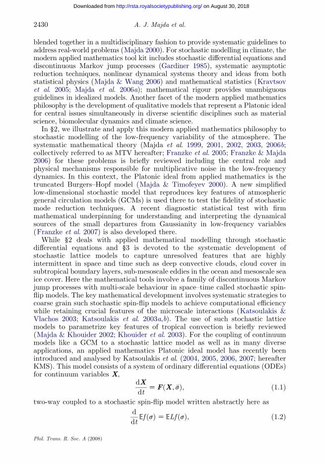
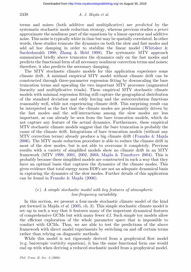
two-time moment KðsÞZhx 02ðtCsÞx 0ðtÞi=hxðtÞ02i3=2, which is a measure ofdeviations from Gaussianity (MTV 2002; Majda et al. 2005). The comparison ofthe reduced model (2.14a) and (2.14b) with the full model (2.13a)–(2.13d ) resultsshows excellent agreement for moderate values of 3Z0.1, 0.5 and still goodagreement for 3Z1.0 (figures 1 and 2). Especially, the non-Gaussian features arereproduced with high accuracy for 3Z0.1 and also 3Z0.5, even though slightlyless well. For large values of 3, the reduced dynamics get the sign of the non-Gaussianity right. All of the reduced models in (2.11)–(2.14a) and (2.14b) cannotbe approximated by the interesting regression strategy of Kravtsov et al. (2005)because there is nonlinear multiplicative noise in (2.13a)–(2.13d ), (2.14a) and(2.14b), nonlinear triad interaction in (2.13a)–(2.13d ) and augmented cubicnonlinearity in (2.14a) and (2.14b). Thus, these regression strategies necessarilyhave large model error in this example.

(f ) A mathematical framework for the mean tendency equationas a dynamical diagnostic

In this section, we provide a general framework to estimate the origin ofnonlinear signatures of planetary wave dynamics and how important the observeddeviations from Gaussianity are for the planetary waves (Franzke et al. 2007).This general framework diagnoses contributions to the mean values of state-dependent tendencies in a low-dimensional subspace of complex geophysicalsystems. The mean phase-space tendencies in some GCMs show distinct nonlinearsignatures in certain planes, which are spanned by its leading EOFs (Selten &Branstator 2004; Branstator & Berner 2005; Franzke et al. 2007) that also show



–1.0

–0.5

0

0.5

1.0(a) (i)

(ii)

(b) (i)

(ii)

(c) (i)

(ii)

auto

corr

elat

ion

func

tion

0 1 2 3 4 5–1.0

–0.5

0

0.5

1.0

time

thir

d-or

der

mom

ent

0 1 2 3 4 5time

0 1 2 3 4 5time

Figure 1. (a–c(i)) Autocorrelation function and (a–c(ii)) third-order moment for different valuesof 3. (a) 3Z1.0, (b) 3Z0.5, and (c) 3Z0.1. Solid lines, full dynamics (2.13a)–(2.13d ) and dashedlines, reduced dynamics (2.14a) and (2.14b).

–1.0

–0.5

0

0.5

1.0

1.5

2.0

2.5

3.0(a) (b)

x2

–1.5 –1.0 – 0.5 0 0.5 1.0 1.5x1 x1

–1.5 –1.0 –0.5 0 0.5 1.0 1.500.10.20.30.40.50.60.70.80.91.0

Figure 2. Joint pdf of the slow modes x 1 and x2 for 3Z0.1. (a) Full dynamics (2.13a)–(2.13d ) and(b) reduced dynamics (2.14a) and (2.14b).



only weak deviations from Gaussianity; mostly in the form of weak skewness andkurtosis and in the case of joint pdfs multiple radial ridges of enhanced density(Franzke & Majda 2006; Berner & Branstator 2007). This mathematicalframework can be applied to complex geophysical systems and reveals how muchthe self-interaction among the modes spanning those planes (climate modes) andhow much the unresolved modes contribute to these mean phase-space tendenciesand also the effect of the observed small deviations from Gaussianity.

To derive the mean tendency equation for the resolved modes, we split thestate vector of a quadratic dynamical system into resolved modes a andunresolved modes b and use conditional mean probability density relations. Notethat while there is a similarity in motivation in decomposing the system into theresolved and unresolved modes compared with the MTV strategy, where the





system is decomposed into the slow and fast modes, the mean tendency equationis more general such that it applies also to systems without time-scale separation.The general formula for the conditional mean tendencies for the dynamics in theresolved variables is derived in Franzke et al. (2007) and is given by

vai

vtja

� �ZFi C

Xj2IR

Lijaj CX

j;k2IR

Bijkajak ; ð2:15aÞ

CXj2IU

Lijhbj jai; ð2:15bÞ

C2X

j2IR;k2IU

Bijkajhbk jai; ð2:15cÞ

CX

j;k2IU

Bijkhbjbkjai: ð2:15dÞ

Note that the r.h.s. of (2.15a) is the bare truncation restricted to interactionsamong the resolved modes, while (2.15b) and (2.15c) involve all of the conditionalmean statistics hbj jai; the terms of (2.15c) are associated with multiplicative triadinteractions (leading to multiplicative noise in an MTV (1999, 2003) frameworkof bj; the terms in (2.15d ) involve all of the conditional interaction statisticshbjbk jai of second moments and include all of the additive triad interactions(leading to additive noise in an MTV framework) of bj and bk. Thus, equation(2.15a)–(2.15d ) provides a general framework to investigate the mean phase-space tendencies, which allows the decomposition into contributions frominteractions among the resolved planetary waves themselves and variouscontributions involving unresolved d.f.

Now we simplify the above conditional mean tendency equation for purelyGaussian EOF modes. The pdfs of EOFs of GCM data are nearly Gaussian(Hsu & Zwiers 2001; Franzke et al. 2005; Franzke &Majda 2006;Majda et al. 2006a;Berner&Branstator 2007) and there aremany geophysicalmodels without dampingand forcing that exactly satisfy these assumptions such as barotropic flow on thesphere with topography (Carnevale & Frederiksen 1987; Salmon 1998; Majda &Wang 2006); thus, it is reasonable as a starting point to assume that the pdf isexactly Gaussian. Thus, in the EOF basis, the pdf factors like

pða; bÞZ PpGi ðaiÞ� �

PpGj ðbjÞ� �

; ð2:16Þ

where pGi ðaiÞ and pGj ðbjÞ are Gaussian distributions with mean zero. Thus, in theGaussian case, the conditional mean tendency equation simplifies to (see Franzkeet al. (2007) for more details)

vai

vtja

� �ZFi C

Xj

Lijaj CXj;k

Bijkajak ð2:17aÞ

CXj

Bijjlj ð2:17bÞ

Note that contributions from (2.15b) and (2.15c), that is, linear coupling andmultiplicative triad interactions, are identically zero.These termsvanishbecause themodes are uncorrelated in theEOFbasis.Thus, in thisGaussian case, the conditionalmean tendency equation recognizes bare truncation (2.15a) and a constant forcing





from additive triad interactions (2.15d ). Since the leading EOFs of GCM data havepdfs with only small, but significant departures from Gaussianity the behaviour in(2.16), (2.17a) and (2.17b) serves as a ‘null hypothesis’ for these deviations fromGaussianity in the climate models.

This general framework predicts that in the case of purely Gaussian modes thenonlinear signatures are stemming from the bare truncation (i.e. the self-interaction among the planetary waves resolved in the low-dimensional plane). InFranzke et al. (2007), these diagnostics were applied to a plane of two low-frequency EOFs in a three-layer climate model with a nonlinear double swirl (seefigure 5a in Franzke et al. 2007); the origin of this double swirl is primarily thethree contributions in (2.15b)–(2.15d ) from the unresolved modes and notnonlinear effects from the bare truncation. The EOFs of the three-layer modelhave small but significant departures from Gaussianity (see figure 9 in Franzkeet al. 2007). Therefore, these deviations account for the contribution of theunresolved onto the resolved modes in the mean phase-space tendencies. Thus,these results show that small deviations from Gaussianity have a substantialimpact on the dynamics of the leading EOFs.

3. Coarse-grained stochastic lattice models for climate:tropical convection

The current practical models for prediction of both weather and climate involveGCMs where the physical equations for these extremely complex flows arediscretized in space and time, and the effects of unresolved processes areparametrized according to various recipes. With the current generation ofsupercomputers, the smallest possible mesh spacings are approximately10–50 km for short-term weather simulations and of order 100 km for short-term climate simulations. There are many important physical processes that areunresolved in such simulations such as the mesoscale sea ice cover, the cloudcover in subtropical boundary layers and deep convective clouds in the tropics.Most of these features are highly intermittent in space and time. An appealingway to represent these unresolved features is through a suitable coarse-grainedstochastic model that simultaneously retains crucial physical features of theinteraction between the unresolved and resolved scales in a GCM. In work from2002 and 2003, two of the authors have developed a new systematic stochasticstrategy (Majda & Khouider 2002; Khouider et al. 2003) to parametrize keyfeatures of deep convection in the tropics involving suitable stochastic spin-flipmodels and also a systematic mathematical strategy to coarse grain suchmicroscopic stochastic models to practical mesoscopic meshes in a computation-ally efficient manner while retaining crucial physical properties of the interaction.

As regards tropical convection, crucial scientific issues involve the fashion inwhich a stochastic model effects the climate mean state and the strength andnature of fluctuations about the climate mean. Here the strategy to develop anew family of coarse-grained stochastic models for tropical deep convection isbriefly reviewed (Majda & Khouider 2002; Khouider et al. 2003) as an illustrativeexample of the potential use of stochastic lattice models. In Khouider et al.(2003), it has been established that in suitable regimes of parameters, the coarse-grained stochastic parametrizations can significantly alter the climatology as well





as increase wave fluctuations about the climatology. This was established inKhouider et al. (2003) in the simplest scenario for tropical climate involving theWalker circulation, the east–west climatological state that arises from localregion of enhanced surface heat flux, mimicking the Indonesian marine continent.Convectively coupled waves in the tropics such as the Madden–Julian oscillationplay an important role in medium-range forecasts, yet the current generation ofcomputer models fails to represent such waves adequately (Lin et al. 2006).Palmer (2001) has emphasized the potential of stochastic parametrization toreduce the model error in a deterministic computer model. Here in an idealizedsetting, we show how to develop a stochastic parametrization to modify andimprove the behaviour of convectively coupled waves in a reasonable prototypeGCM; this is achieved by following a path guided by the systematic designprinciple for the idealized model in (1.1) (KMS 2006, 2007) to build in suitableintermittency effects.

(a ) The microscopic stochastic model for convective inhibition

In a typical GCM, the fluid dynamical and thermodynamical variablesdenoted here by the generic vector u are regarded as known only over a discretehorizontal mesh with ujZuðjDx; tÞ denoting these discrete values. Throughoutthe discussion, one horizontal spatial dimension along the equator in the east–west direction is assumed for simplicity in notation and explanation. Asmentioned above, the typical mesh spacing in a GCM is coarse with Dx rangingfrom 50 to 250 km depending on the time duration of the simulation. Thestochastic variable used to illustrate the approach is convective inhibition (CIN).Observationally, CIN is known to have significant fluctuations on a horizontalspatial scale on the order of a kilometre, the microscopic scale here, with changesin CIN attributed to different mechanisms in the turbulent boundary layer, suchas gust fronts, gravity waves and turbulent fluctuations in equivalent potentialtemperature (Mapes 2000). In Majda & Khouider (2002) and Khouider et al.(2003), it was proposed that all of these different microscopic physicalmechanisms and their interaction that increase and decrease CIN are toocomplex to model in detail in a coarse-mesh GCM parametrization and instead,as in statistical mechanics, should be modelled by a simple order parameter sI,taking only two discrete values,

sI Z 1 at a site if convection is inhibited ða CIN siteÞsI Z 0 at a site if there is potential for deep convection ða PAC siteÞ:

)ð3:1Þ

The value of CIN at a given coarse-mesh point is determined by the averagingof CIN over the microscopic states in the vicinity of the given mesh point, i.e.

�sIð jDx; tÞZ1

Dx

ððjC1=2ÞDx

ðjK1=2ÞDxsIðx; tÞ dx: ð3:2Þ

Note that the mesh size Dx is mesoscopic, that is, between the microscaleO(1 km) and the macroscale O(10 000 km), and that �sI can have any value in therange 0% �sI%1. Discrete sums over microscopic mesh values (of order 1 km)and continuous integrals are used interchangeably for notational convenience(Majda & Khouider 2002).





(b ) The simplest coarse-grained stochastic model

In practical parametrization, it is desirable for computational feasibility toreplace the microscopic dynamics by a process on the coarse mesh, which retainscritical dynamical features of the interaction. Following the general proceduredeveloped and tested in Katsoulakis & Vlachos (2003) and Katsoulakis et al.(2003a,b), the simplest local version of the systematic coarse-grained stochasticprocess is developed in Khouider et al. (2003) and summarized here.

Each coarse cell Dxk, kZ1,., m, of the coarse-grained lattice is divided into qmicroscopic cells, such that Dxkh1/q {1, 2,., q}, kZ1,., m. In the coarse-grained procedure, given the coarse-grained sequence of random variables

htðkÞZX

y2Dxk

sI;tðyÞ; ð3:3Þ

so that the average in (3.2) verifies �sIðjDxÞZhðkÞ=q, for jZk in some sense, themicroscopic dynamics is replaced by a birth/death Markov process defined onthe variables {0, 1,., q} for each k, such that ht(k) evolves according to thefollowing probability law:

Prob fhtCDtðkÞZ nC1jhtðkÞZngZCaðk;nÞDtCoðDtÞProb fhtCDtðkÞZ nK1jhtðkÞZngZCdðk; nÞDtCoðDtÞProb fhtCDtðkÞZ njhtðkÞZngZ 1KðCaðk;nÞCCdðk; nÞÞDtCoðDtÞProb fhtCDtðkÞsn; nK1; nC1jhtðkÞZngZ oðDtÞ:

9>>>>=>>>>;

ð3:4Þ

Here Ca andCd are the coarse-grained adsorption and desorption rates representingthe rates at which CIN sites are being created and destroyed, respectively, withinone coarse-grained cell, that is, the birth/death rates for the Markov process is

Caðk;hÞZ1

tI½qKhðkÞ�;

Cdðk;hÞZ1

tIhðkÞeKb �V ðkÞ;

9>>>=>>>;

ð3:5Þ

where�V ðkÞZ �J ð0; 0ÞðhðkÞK1ÞChext; ð3:6Þ

with the coarse-grained interaction potential within the coarse cell given by�J ð0; 0ÞZ2U0=ðqK1Þ, whereU0 is themean strength of the microscopic interactionpotential J between neighbouring sites (Katsoulakis et al. 2003a,b). The coarse-grained energy content for CIN is given by the coarse-grained Hamiltonian

�HðhÞZ U0

qK1

Xk

hðkÞðhðkÞK1ÞChextXk

hðkÞ; ð3:7Þ

where hext is the external potential that modifies the energy for CIN depending onthe large-scale flow variables. The canonical invariant Gibbs measure for the coarse-grained stochastic process is a product measure given by

Gm;q;bðhÞZ ðZm;q;bÞK1eb�H ðhÞPm;qðdhÞ; ð3:8Þ

where Pm;qðdhÞ is a given explicit/prior distribution (Katsoulakis et al. 2003b). Asshown in Katsoulakis et al. (2003b), the coarse-grained birth/death process abovesatisfies detailed balance with respect to the Gibbs measure in (3.8) as well as a





number of other attractive theoretical features. The simplest coarse-grainedapproximation given above assumes that the effect of the microscopic interactionson the mesoscopic scales occurs within the mesoscopic coarse-mesh scale Dx,otherwise systematic non-local couplings are needed (Katsoulakis et al. 2003b). Theaccuracy of these approximations is tested for diverse examples from materialscience elsewhere (Katsoulakis & Vlachos 2003; Katsoulakis et al. 2003a,b) and forthe instructive idealized coupled models in (1.1) (KMS 2004, 2005, 2006, 2007).

The practical implementation of the coarse-grained birth/death process in(3.3)–(3.6) requires specification of the parameters, tI, U0, q and the externalpotential hextðujÞ as well as the statistical parameter b. The advantages of such astochastic lattice model are as follows:

— retains systematically the energetics of unresolved features through thecoarse-grained Gibb’s measure;

—has minimal computational overhead since there are rapid algorithms forupdating birth–death processes;

— incorporates feedbacks of the resolved modes on the unresolved modes andtheir energetics through an external field; and

— includes dynamical coupling through not only sampling the probabilitydistributions of unresolved variables but also their evolving behaviour in timeis constrained by the large-scale dynamics.

(c ) The model deterministic convective parametrization

A prototype mass flux parametrization with crude vertical resolution(Majda & Shefter 2001; Khouider & Majda 2006b) is used to illustrate thefashion in which the coarse-grained stochastic model for CIN can be coupled to adeterministic convective mass flux parametrization. The prognostic variablesðu; q; qeb; qemÞ are the x -component of the fluid velocity, u, the potentialtemperature in the middle troposphere, q, the equivalent potential temperatures,qeb and qem, measuring the potential temperatures plus moisture content of theboundary layer and middle troposphere, respectively. The vertical structure isdetermined by projection on a first baroclinic heating mode (Majda & Shefter2001; Khouider & Majda 2006b). The dynamic equations for these variables inthe parametrization are given by

vu

vtK ��a

vq

vxZK C 0

D

1

h

ffiffiffiffiffiffiffiffiffiffiffiffiffiffiffiffiu20 Cu2

q !uK

1

tDu;

vq

vtK �a

vu

vxZSKQ0

RKq

tR;

hvqeb

vtZKDðqebK qemÞC Cq

ffiffiffiffiffiffiffiffiffiffiffiffiffiffiffiffiu20Cu2

q� �ðq�ebK qebÞ;

Hvqem

vtZDðqebK qemÞKHQ0

RKHqem

tR;

9>>>>>>>>>>>>>>>=>>>>>>>>>>>>>>>;

ð3:9Þ





while the constants Q 0R and q�

eb are externally imposed and represent theradiative cooling at equilibrium in the upper troposphere and saturationequivalent potential temperature in the boundary layer. The constants h andH measure the depths of the boundary layer and the troposphere above theboundary layer, respectively. The typical values used here are hZ500 m and

HZ16 km, while u0Z2 m sK1 and C 0DZ0:001, corresponding to a momentum

spin up time of approximately 3 days. The explicit values for the other constantsused in (3.9) and elsewhere in this section can be found in Majda & Shefter(2001) and Khouider et al. (2003).

The crucial quantities in the prototype mass flux parametrization are theterms S and D, where S represents the middle troposphere heating due to deepconvection, while D represents the downward mass flux on the boundary layer.The heating term S is given by

S ZMscððCAPEÞCÞ1=2; ð3:10Þ

where M is a fixed constant; sc is the area fraction for deep convective mass flux;and CAPEZRðqebKgqÞ is the convectively available potential energy. Here R isa dimensional constant (Majda & Shefter 2001; Khouider et al. 2003). Thedownward mass flux on the boundary layer D includes the environmentaldowndrafts me and the downward mass flux due to convection mK, which arenon-negative quantities with explicit formulae described elsewhere (Majda &Shefter 2001; Khouider et al. 2003). The notation (X )C denotes the positive partof X. This parametrization respects conservation of vertically integrated moiststatic energy.

The equations (3.9) and (3.10) represent an idealized GCM with crude verticalresolution based on a reasonable design principle for deep convection includingbasic conservation principles. However, like the current generation of GCMs, themodel has major deficiencies as regards convectively coupled waves. First,instabilities for the full model in (3.9) arise only through the nonlinearity fromffiffiffiffiffiffiffiffiffiffiffiffiffiffiffiffiu20Cu2

qand are called the wind-induced surface heat exchange (WISHE)

instability (Majda & Shefter 2001, and references therein). Second, if the bulk

aerodynamic flux coefficients in (3.9),ffiffiffiffiffiffiffiffiffiffiffiffiffiffiffiffiu20Cu2

qare replaced by the constant

value ju0j, that is no WISHE, all waves in the system are stable and nofluctuations emerge in an aquaplanet simulation (Majda & Shefter 2001). Thereis no observational evidence supporting the role of WISHE in driving the large-scale convectively coupled waves in nature (Lin et al. 2006 and referencestherein); here the WISHE term is regarded as a deterministic fix in a GCMparametrization to generate instabilities. The simulation results reported infigure 5a show that in an aquaplanet model above the equator, two regularperiodic convectively coupled waves moving eastward and westward at roughlyequal strength are generated by the idealized GCM. Since GCMs often haveconvectively coupled waves that move too fast and are too regular (Lin et al.2006), the goal here is to see whether the stochastic lattice coupling will slowdown the waves in the deterministic parametrization and simultaneouslyincrease the spatio-temporal fluctuations in those waves. It is important tonote here that there are recent deterministic multicloud models (Khouider &Majda 2006a, 2007, 2008) for convectively coupled waves involving the three cloud





types in observations above the boundary layer, congestus, deep and stratiform,and their heating structure that reproduces key features of the observationalrecord for convectively coupled waves (Lin et al. 2006). The mechanism ofinstability in these models (Khouider & Majda 2006a) is completely differentfrom WISHE that is not active in the multicloud models. For the idealizedsetting of flow above the equator, the multicloud models can produce packets ofconvectively coupled waves moving in one direction at 15–20 m sK1 with theirlow-frequency envelopes moving at 4–7 m sK1 in the opposite direction across thewarm pool in a fashion like the Madden–Julian oscillation (Khouider & Majda2007, 2008).

(d ) Coupling of the stochastic CIN model into the parametrization

The equations (3.9) and (3.10) are regarded here as the prototypedeterministic GCM parametrization when discretized in a standard fashionusing central differences on a coarse mesh Dx with Dx ranging from 50 to 250 km.In the simulations from Khouider et al. (2003), and those presented below,DxZ80 km. The coarse-grained stochastic CIN model is coupled to this basicparametrization. The area fraction for deep convection sc governing the upwardmass flux strength is allowed to vary on the coarse mesh and is given by

scð jDxÞZ 1K�sIðjDxÞ½ �sCc ; ð3:11Þwhere �sI is the average in (3.2) and sCc is a threshold constant and equal to 0.002(Majda & Shefter 2001; Khouider et al. 2003). When the order parameter sIsignifies strong CIN locally so that �sIZ1 the flux of deep convection isdiminished to zero while with PAC locally active �sIZ0, this flux increases to themaximum allowed by the value sCc . To complete the coupling of the stochasticCIN model into the parametrization, the coarse-mesh external potential h extðujÞ,from (3.6) and (3.7), needs to be specified from the coarse-mesh values uj. Thereis no unique choice of the external potential but its form can be dictated bysimple physical reasoning. In Khouider et al. (2003), the plausible physicalassumption is made that when the convective downward mass flux mK decreasesthe energy for CIN decreases. Since the convective downward mass flux resultsfrom the evaporative cooling induced by precipitation falling into dry air, itconstitutes a mechanism that carries negatively buoyant cool and dry air fromthe middle troposphere onto the boundary layer, hence tending to reduce CAPEand deep convection.

Another natural external potential is the boundary-layer equivalent potential,since the flux at the boundary is crucial physically. As such, it yields somewhatstronger and more intermittent fluctuations. Thus, the choice

h extð jDx; tÞZ ~gqebð jDx; tÞ ð3:12Þis used here with ~g a calibration factor. The other parameters in the stochasticlattice model are chosen as tIZ2 hours, bZ1, U0Z1 so that CIN sites arefavoured in the equilibrium Gibbs measure.

(e ) The stochastic single-column model and intermittency

A central issue is how to calibrate the stochastic lattice model to generateintermittent fluctuations with plausible magnitudes as observed in tropical



0 0.2 0.4

βJ0 = 1, γt = 0.1

0.6CIN: Σγ

0.8 1.0

1

2

3

4

Cd/C

a

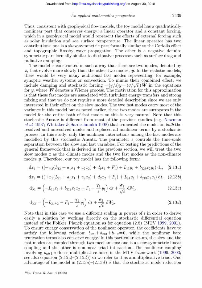
Figure 3. Ratio of the adsorption and desorption rates Cd/Ca for the birth–death stochastic latticemodel with parameters ~gZ0:1, bZU0Z1 and a number of microscopic sites qZ10 (green), qZ100(red) and qZ1000 (blue). Note that a CIN-dominating equilibrium with large CIN values yieldlarge PAC (adsorption) rates. The balanced equilibrium curve Cd/CaZ1 is shown. Arrows indicateoverall tendency of CIN coverage.



convection. A natural design framework is first to achieve such behaviour in thestochastic single-column model given by the following equations:

dq

dtZ ð1K sIÞM

ffiffiffiffiffiffiffiffiffiffiffiffiffiffiffiffiffiffiffiffiffiffiffiffiffiffiffiRðqebKgqÞC

qKQ0

RK1

tRq;

dqebdt

ZK1

tebð1K sIÞ


qðqebK qemÞC

1

teq�ebK qemð Þ;

dqemdt

Z1

temð1K sIÞ


qðqebK qemÞK

1

tRq;

9>>>>>>>>>=>>>>>>>>>;

ð3:13Þ

Here sI is computed from the birth–death stochastic model in (3.3)–(3.6) withthe interaction potential defined through qeb from (3.7) and the definition of hext

in (3.12) above. The different time scales were computed for a radiativeconvective equilibrium consistent with the Jordan tropical sounding and thevalues tebz6 hours, temz8 days, tez8 hours, Q 0

RZ1 K dK1, tRZ50 days andtDZ75 days are used here (Khouider et al. 2003). This is a specific example ofthe prototype models from (1.1) studied extensively in idealized settings (KMS2004, 2005, 2006). As mentioned earlier, the choices bZ1, U0Z1 guarantee thatthe Gibbs measure in (3.8) has a high probability for CIN states; this is a naturalrequirement for deep convection, where the area fraction of deep convection ismuch smaller than the area with positive CAPE. In order to generateintermittency and fluctuations in the stochastic column model, it is very naturalto require that the ratio of the creation rate of PAC sites to the creation rate ofCIN sites, Cd/Ca, becomes large as sIb1 (KMS 2006, 2007). In figure 3, it isshown that this property of the stochastic model is satisfied for the coefficient~gZ0:1 in the external potential in (3.12) with similar behaviour for qZ10,



40.5

41.0

41.5(a)

(b)

(c)

(d )

(e)

68

70

72

74

47.5

48.0

48.5

0

0.5

1.0

0 20 40 60 80 100 120 140 160 180 200

0.05

0.10

time (days)

mas

s fl

ux:

cWc

(m s

–1)

Figure 4. (a–e) Time series of dynamical variables for the stochastic single-column model withtIZ2 hours, ~gZ0:1, bZU0Z1, qZ10. Note the manifestation of strong intermittent bursts beyondthe stochastically generated CIN; especially, in qeb and mass flux scWc hð1KsIÞ

ffiffiffiffiffiffiffiffiffiffiffiffiffiffiffiffiffiffiffiffiffiffiffiffiffiffiRðqebKgq1Þ

p.

The deterministic equilibrium value is represented by the horizontal line on each panel.



100 and 1000. Recall that q is the number of microscopic states in the birth–death process. A time series of the stochastic column model implemented withthese parameters is displayed in figure 4 with qZ10. The strongly intermittentfluctuations in qeb over several degrees Kelvin as well as similar intermittency inthe mass flux is evident. They are consistent with SST variations observed in theIndian Ocean warm pool (e.g. Fasullo & Webster 1999). Also note that thefluctuations in the mid-troposphere potential temperature are much weaker inmagnitude as occurs in the actual tropics, where middle tropospherictemperature anomalies are on the order of 0.1–0.58C (e.g. Wheeler et al. 2000).

(f ) The effects of the stochastic parametrization on convectively coupled waves

All parameters in the stochastic lattice model have been determined throughsystematic design principles in the previous section. Here the results of numericalsimulations of the stochastic model in statistical steady state are reported for



0 5 10 15 20 25 30 35

230

240

250

260

270

280

290

300

110120130140150160170

200190180

(a) (b)

(c)

15 m s–1

X (1000 km)

time

(day

s)

m s

–1

–3.0–2.5–2.0–1.5–1.0–0.500.51.01.52.0

0 5 10 15 20 25 30 35

11 m s–1

X (1000 km)

–3

–2

–1

0

1

2

3

4

X (1000 km)

time

(day

s)

0 5 10 15 20 25 30 35 40

230

240

250

260

270

280

290

300

–1.0–0.8–0.6–0.4–0.200.20.40.60.81.0

8 m s–1

Figure 5. Effect of the birth–death stochastic CIN on large scale convectively coupled waves withthe stochastic parameters bZU0Z1, qZ10. (a) Purely deterministic WISHE waves without thestochastic coupling, (b) effect of stochastic CIN on WISHE waves, (c) intermittent bursts ofconvective episodes with apparent tracks of waves maintained by the stochastic CIN effectsalone—WISHE is OFF. The apparent speed of propagation is shown by the dashed lines. Notethe different time scales in (b) compared with (a,c). Space–time velocity contours are shownas indicated.



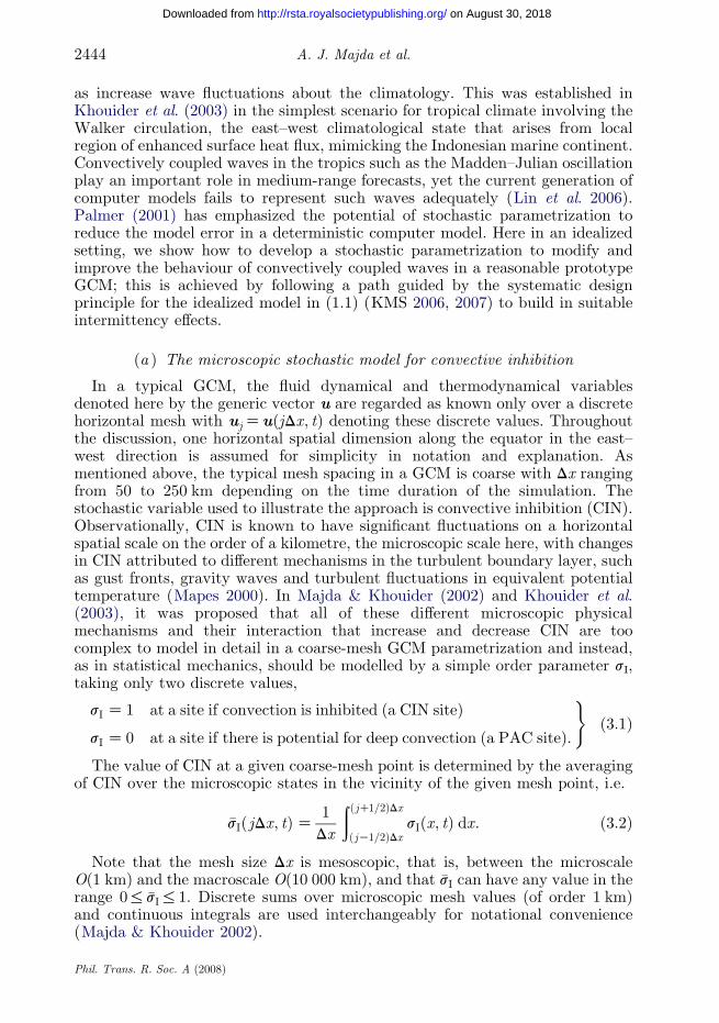
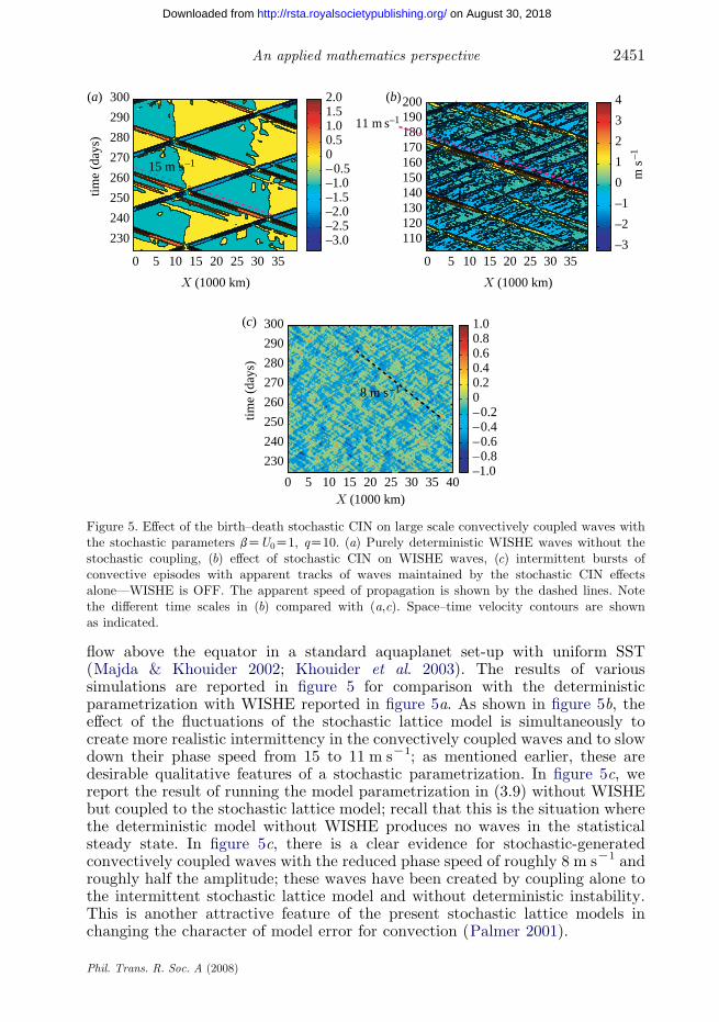
flow above the equator in a standard aquaplanet set-up with uniform SST(Majda & Khouider 2002; Khouider et al. 2003). The results of varioussimulations are reported in figure 5 for comparison with the deterministicparametrization with WISHE reported in figure 5a. As shown in figure 5b, theeffect of the fluctuations of the stochastic lattice model is simultaneously tocreate more realistic intermittency in the convectively coupled waves and to slowdown their phase speed from 15 to 11 m sK1; as mentioned earlier, these aredesirable qualitative features of a stochastic parametrization. In figure 5c, wereport the result of running the model parametrization in (3.9) without WISHEbut coupled to the stochastic lattice model; recall that this is the situation wherethe deterministic model without WISHE produces no waves in the statisticalsteady state. In figure 5c, there is a clear evidence for stochastic-generatedconvectively coupled waves with the reduced phase speed of roughly 8 m sK1 androughly half the amplitude; these waves have been created by coupling alone tothe intermittent stochastic lattice model and without deterministic instability.This is another attractive feature of the present stochastic lattice models inchanging the character of model error for convection (Palmer 2001).





4. Concluding remarks

This paper both reviewed and provided new illustrations and examples ofthe fashion in which modern applied mathematics can provide new perspectivesand systematic design principles for stochastic modelling for climate. Section 2was devoted to systematic stochastic modelling of low-frequency variabilityincluding the quantitative sources for multiplicative noise. A new simplified low-dimensional stochastic model with key features of atmospheric low-frequencyvariability was introduced in §2e in order to test stochastic mode reductionstrategies. A recent diagnostic test with firm mathematical underpinning forexploring the subtle departures from Gaussianity and their sources was discussedin §2f. Section 3 was devoted to developing stochastic lattice models to captureintermittent features and improve the fidelity of deterministic parametrizations.Recent systematic design principles (KMS 2006, 2007) were used to calibrate astochastic column model for tropical convection in §3e; the practical effect ofslowing down convectively coupled waves and increasing their fluctuationsthrough these stochastic lattice models was presented in §3f.

The authors thank their collaborators, Eric Vanden-Eijnden, Ilya Timofeyev, Markos Katsoulakisand Alex Sopasakis, for their explicit and implicit contributions to the work presented here. Theresearch of A.J.M. is partially funded by the National Science Foundation grant no. DMS-0456713,the Office of Naval Research grant no. N00014-05-1-0164 and the Defense Advanced ResearchProject Agency grant no. N00014-07-1-0750. The research of B.K. is partly supported by a grantfrom the National Sciences and Engineering Research Council of Canada.

References

Achatz, U. & Branstator, G. 1999 A two-layer model with empirical linear corrections and reducedorder for studies of internal climate variability. J. Atmos. Sci. 56, 3140–3160. (doi:10.1175/1520-0469(1999)056!3140:ATLMWEO2.0.CO;2)

Achatz, U. & Opsteegh, J. D. 2003a Primitive-equation-based low-order models with seasonalcycle. Part I: model construction. J. Atmos. Sci. 60, 465–477. (doi:10.1175/1520-0469(2003)060!0465:PEBLOMO2.0.CO;2)

Achatz, U. & Opsteegh, J. D. 2003b Primitive-equation-based low-order models with seasonalcycle. Part II: application to complexity and nonlinearity of large-scale atmosphere dynamics.J. Atmos. Sci. 60, 478–490. (doi:10.1175/1520-0469(2003)060!0478:PEBLOMO2.0.CO;2)

Berner, J. 2005 Linking nonlinearity and non-Gaussianity of planetary wave behaviour by theFokker–Planck equation. J. Atmos. Sci. 62, 2098–2117. (doi:10.1175/JAS3468.1)

Berner, J. & Branstator, G. 2007 Linear and nonlinear signatures in the planetary wave dynamics of anAGCM: probability density functions. J. Atmos. Sci. 64, 117–136. (doi:10.1175/JAS3822.1)

Branstator, G. 1990 Low-frequency patterns induced by stationary waves. J. Atmos. Sci. 47,629–648. (doi:10.1175/1520-0469(1990)047!0629:LFPIBSO2.0.CO;2)

Branstator, G. & Berner, J. 2005 Linear and nonlinear signatures in the planetary wave dynamicsof an AGCM: phase space tendencies. J. Atmos. Sci. 62, 1792–1811. (doi:10.1175/JAS3429.1)

Branstator, G. & Haupt, S. E. 1998 An empirical model of barotropic atmospheric dynamicsand its response to tropical forcing. J. Clim. 11, 2645–2667. (doi:10.1175/1520-0442(1998)011!2645:AEMOBAO2.0.CO;2)

Carnevale, G. & Frederiksen, J. S. 1987 Nonlinear stability and statistical mechanics for flow overtopography. J. Fluid Mech. 175, 157–181. (doi:10.1017/S002211208700034X)

Crommelin, D. T. & Majda, A. J. 2004 Strategies for model reduction: comparing differentoptimal bases. J. Atmos. Sci. 61, 2206–2217. (doi:10.1175/1520-0469(2004)061!2206:SFMRCDO2.0.CO;2)


http://dx.doi.org/doi:10.1175/1520-0469(1999)056%3C3140:ATLMWE%3E2.0.CO;2

http://dx.doi.org/doi:10.1175/1520-0469(1999)056%3C3140:ATLMWE%3E2.0.CO;2

http://dx.doi.org/doi:10.1175/1520-0469(2003)060%3C0465:PEBLOM%3E2.0.CO;2



http://dx.doi.org/doi:10.1175/JAS3468.1


http://dx.doi.org/doi:10.1175/1520-0469(1990)047%3C0629:LFPIBS%3E2.0.CO;2


http://dx.doi.org/doi:10.1175/1520-0442(1998)011%3C2645:AEMOBA%3E2.0.CO;2

http://dx.doi.org/doi:10.1175/1520-0442(1998)011%3C2645:AEMOBA%3E2.0.CO;2

http://dx.doi.org/doi:10.1017/S002211208700034X

http://dx.doi.org/doi:10.1175/1520-0469(2004)061%3C2206:SFMRCD%3E2.0.CO;2

http://dx.doi.org/doi:10.1175/1520-0469(2004)061%3C2206:SFMRCD%3E2.0.CO;2




Crommelin, D. T. & Vanden-Eijnden, E. 2006 Reconstruction of diffusion using spectral data from

timeseries. Comm. Math. Sci. 4, 651–668.

Delsole, T. 2004 Stochastic models of quasi-geostrophic turbulence. Surv. Geophys. 25, 107–149.

(doi:10.1023/B:GEOP.0000028164.58516.b2)

Egger, J. 2005 A stochastic model for the angular momentum budget of latitude belts. J. Atmos.

Sci. 62, 2592–2601. (doi:10.1175/JAS3480.1)

Fasullo, J. & Webster, P. 1999 Warm pool SST variability in relation to the surface energy

balance. J. Clim. 12, 1292–1305. (doi:10.1175/1520-0442(1999)012!1292:WPSVIRO2.0.CO;2)

Feldstein, S. B. 2000 The timescale, power spectra, and climate noise properties of teleconnection

patterns. J. Clim. 13, 4430–4440. (doi:10.1175/1520-0442(2000)013!4430:TTPSACO2.0.CO;2)

Franzke, C. & Majda, A. J. 2006 Low-order stochastic mode reduction for a prototype atmospheric

GCM. J. Atmos. Sci. 63, 457–479. (doi:10.1175/JAS3633.1)

Franzke, C., Majda, A. J. & Vanden-Eijnden, E. 2005 Low-order stochastic mode reduction for a

realistic barotropic model climate. J. Atmos. Sci. 62, 1722–1745. (doi:10.1175/JAS3438.1)

Franzke, C., Majda, A. J. & Branstator, G. 2007 The origin of nonlinear signatures of planetary

wave dynamics: mean phase space tendencies and contributions from non-Gaussianity.

J. Atmos. Sci. 64, 3987–4003. (doi:10.1175/2006JAS2221.1)

Frederiksen, J. S., Dix, M. R. & Kepert, S. M. 1996 Systematic energy errors and the tendency

toward canonical equilibrium in atmospheric circulation models. J. Atmos. Sci. 53, 887–904.

(doi:10.1175/1520-0469(1996)053!0887:SEEATTO2.0.CO;2)

Gardiner, C. W. 1985. Handbook of stochastic methods, p. 442, Berlin, Germany: Springer.

Hasselmann, K. 1988 PIPs and POPs: the reduction of complex dynamical systems using principal

interaction and oscillation patterns. J. Geophys. Res. 93, 11 015–11 021. (doi:10.1029/

JD093iD09p11015)

Hsu, C. J. & Zwiers, F. 2001 Climate change in recurrent regimes and modes of northern

hemisphere atmospheric variability. J. Geophys. Res. 106, 20 145–20 159. (doi:10.1029/

2001JD900229)

Hurrell, J. W. 1995 Decadal trends in the north atlantic oscillation: regional temperatures and

precipitation. Science 269, 676–679. (doi:10.1126/science.269.5224.676)

Katsoulakis, M. A. & Vlachos, G. D. 2003 Hierarchical kinetic Monte Carlo simulations for

diffusion of interacting molecules. J. Chem. Phys. 112, 9412–9427. (doi:10.1063/1.1616513)

Katsoulakis, M. A., Majda, A. J. & Vlachos, G. D. 2003a Coarse-grained stochastic processes for

microscopic lattice systems. Proc. Natl Acad. Sci. USA 100, 782–787. (doi:10.1073/pnas.

242741499)

Katsoulakis, M. A., Majda, A. J. & Vlachos, G. D. 2003b Coarse-grained stochastic processes and

Monte Carlo simulations in lattice systems. J. Comp. Phys. 186, 250–278. (doi:10.1016/S0021-

9991(03)00051-2)

Katsoulakis, M. A., Majda, A. J. & Sopasakis, A. 2004 Multiscale coupling in prototype hybrid

deterministic/stochastic systems. Part I: deterministic closures. Comm. Math. Sci. 2, 255–294.

Katsoulakis, M. A., Majda, A. J. & Sopasakis, A. 2005 Multiscale coupling in prototype hybrid

deterministic/stochastic systems. Part II: stochastic closures. Comm. Math. Sci. 3, 453–478.

Katsoulakis, M. A., Majda, A. J. & Sopasakis, A. 2006 Intermittency, metastability, and coarse

graining for coupled deterministic–stochastic lattice systems. Nonlinearity. 19, 1021–1047.

(doi:10.1088/0951-7715/19/5/002)

Katsoulakis, M. A., Majda, A. J. & Sopasakis, A. 2007 Prototype hybrid couplings of macroscopic

deterministic models and microscopic stochastic lattice dynamics. Contemp. Math. 429, 143–187.

Khouider, B. & Majda, A. J. 2006a A simple multicloud parametrization for convectively coupled

tropical waves. Part I: linear analysis. J. Atmos. Sci. 63, 1308–1323. (doi:10.1175/JAS3677.1)

Khouider, B. & Majda, A. J. 2006b Model multicloud parametrizations with crude vertical

structure. Theor. Comp. Fluid Dyn. 20, 351–375. (doi:10.1007/s00162-006-0013-2)

Khouider, B. & Majda, A. J. 2007 A simple multicloud parametrization for convectively coupled

tropical waves. Part II: nonlinear simulations. J. Atmos. Sci. 64, 381–400. (doi:10.1175/JAS3833.1)


http://dx.doi.org/doi:10.1023/B:GEOP.0000028164.58516.b2


http://dx.doi.org/doi:10.1175/1520-0442(1999)012%3C1292:WPSVIR%3E2.0.CO;2

http://dx.doi.org/doi:10.1175/1520-0442(2000)013%3C4430:TTPSAC%3E2.0.CO;2



http://dx.doi.org/doi:10.1175/2006JAS2221.1

http://dx.doi.org/doi:10.1175/1520-0469(1996)053%3C0887:SEEATT%3E2.0.CO;2

http://dx.doi.org/doi:10.1029/JD093iD09p11015

http://dx.doi.org/doi:10.1029/JD093iD09p11015

http://dx.doi.org/doi:10.1029/2001JD900229

http://dx.doi.org/doi:10.1029/2001JD900229

http://dx.doi.org/doi:10.1126/science.269.5224.676

http://dx.doi.org/doi:10.1063/1.1616513

http://dx.doi.org/doi:10.1073/pnas.242741499


http://dx.doi.org/doi:10.1016/S0021-9991(03)00051-2

http://dx.doi.org/doi:10.1016/S0021-9991(03)00051-2

http://dx.doi.org/doi:10.1088/0951-7715/19/5/002


http://dx.doi.org/doi:10.1007/s00162-006-0013-2





Khouider, B. & Majda, A. J. 2008 Multicloud models for tropical convection: enhanced congestus

heating. J. Atmos. Sci. 65, 895–914. (doi:10.1175/2007JAS2408.1)Khouider, B., Majda, A. J. & Katsoulakis, M. 2003 Coarse grained stochastic models for tropical

convection. Proc. Natl Acad. Sci. USA 100, 11 941–11 946. (doi:10.1073/pnas.1634951100)Kravtsov, S., Kondrashov, D. & Ghil, M. 2005 Multi-level regression modeling of nonlinear

processes: derivation and applications to climate variability. J. Clim. 62, 4404–4424. (doi:10.

1175/JCLI3544.1)Kurtz, T. G. 1973 A limit theorem for perturbed operators semigroups with applications to random

evolution. J. Funct. Anal. 12, 55–67. (doi:10.1016/0022-1236(73)90089-X)Kwasniok, F. 1996 The reduction of complex dynamical systems using principal interaction

patterns. Physica D 92, 28–60. (doi:10.1016/0167-2789(95)00280-4)Kwasniok, F. 2004 Empirical low-order models of barotropic flow. J. Atmos. Sci. 61, 235–245.

(doi:10.1175/1520-0469(2004)061!0235:ELMOBFO2.0.CO;2)Lin, J.-L., Kiladis, G. N., Mapes, B. E., Weickmann, K. M., Sperber, K. R., Lin, W., Wheeler, M.,

Roeckner, S. D. & Scinocca, J. F. 2006 Tropical intraseasonal variability in 14 IPCC AR4

climate models. Part 1: convective signals. J. Clim. 19, 2665–2690. (doi:10.1175/JCLI3735.1)Majda, A. J. 2000 Real world turbulence and modern applied mathematics. In Mathematics frontiers

and perspectives (ed. V. Arnold), pp. 137–151. Providence, RI: American Mathematical Society.Majda, A. J. & Khouider, B. 2002 Stochastic and mesoscopic models for tropical convection. Proc.

Natl Acad. Sci. USA 99, 1123–1128. (doi:10.1073/pnas.032663199)Majda,A. J.&Shefter,M. 2001Waves and instabilities formodel tropical convective parametrizations.

J. Atmos. Sci. 58, 896–914. (doi:10.1175/1520-0469(2001)058!0896:WAIFMTO2.0.CO;2)Majda, A. J. & Timofeyev, I. 2000 Remarkable statistical behavior for truncated Burgers-Hopf

dynamics. Proc. Natl Acad. Sci. USA 97, 12 413–12 417. (doi:10.1073/pnas.230433997)Majda, A. J. & Timofeyev, I. 2004 Low dimensional chaotic dynamics versus intrinsic stochastic

chaos: a paradigm model. Physica D 199, 339–368. (doi:10.1016/j.physd.2004.05.012)Majda, A. J. and Wang, X. 2006 Nonlinear dynamics and statistical theories for basic geophysical

flows, p. 600. Cambridge, UK: Cambridge University Press.Majda, A. J., Timofeyev, I. & Vanden-Eijnden, E. 1999 Models for stochastic climate prediction.

Proc. Natl Acad. Sci. USA 96, 14 687–14 691. (doi:10.1073/pnas.96.26.14687)Majda, A. J., Timofeyev, I. & Vanden-Eijnden, E. 2001 A mathematical framework for stochastic

climate models. Commun. Pure Appl. Math. 54, 891–974. (doi:10.1002/cpa.1014)Majda, A. J., Timofeyev, I. & Vanden-Eijnden, E. 2002 A priori tests of a stochastic mode

reduction strategy. Physica D 170, 206–252. (doi:10.1016/S0167-2789(02)00578-X)Majda, A. J., Timofeyev, I. & Vanden-Eijnden, E. 2003 Systematic strategies for stochastic mode

reduction in climate. J. Atmos. Sci. 60, 1705–1722. (doi:10.1175/1520-0469(2003)060!1705:

SSFSMRO2.0.CO;2)Majda, A. J., Abramov, R. & Grote, M. 2005 Information theory and stochastics for multiscale

nonlinear systems. Monograph Series of Center for Research in Mathematics, University ofMontreal, p. 140. Providence, RI: American Mathematical Society.

Majda, A. J., Franzke, C., Fischer, A. & Crommelin, D. T. 2006a Distinct metastable atmosphericregimes despite nearly Gaussian statistics: a paradigm model. Proc. Natl Acad. Sci. USA 103,

8309–8314. (doi:10.1073/pnas.0602641103)Majda, A. J., Timofeyev, I. & Vanden-Eijnden, E. 2006b Stochastic models for selected slow variables

in large deterministic systems. Nonlinearity 19, 769–794. (doi:10.1088/0951-7715/19/4/001)Mapes, B. E. 2000 Convective inhibition, subgridscale triggering energy, and “stratiform

instability” in a toy tropical wave model. J. Atmos. Sci. 57, 1515–1535. (doi:10.1175/1520-

0469(2000)057!1515:CISSTEO2.0.CO;2)Marshall, J. & Molteni, F. 1993 Toward a dynamical understanding of planetary-scale flow regimes.

J. Atmos. Sci. 50, 1792–1818. (doi:10.1175/1520-0469(1993)050!1792:TADUOPO2.0.CO;2)Newman, M., Sardeshmukh, P. D. & Penland, C. 1997 Stochastic forcing of the wintertime

extratropical flow. J. Atmos. Sci. 54, 435–455. (doi:10.1175/1520-0469(1997)054!0435:SFOT-WEO2.0.CO;2)


http://dx.doi.org/doi:10.1175/2007JAS2408.1


http://dx.doi.org/doi:10.1175/JCLI3544.1


http://dx.doi.org/doi:10.1016/0022-1236(73)90089-X

http://dx.doi.org/doi:10.1016/0167-2789(95)00280-4

http://dx.doi.org/doi:10.1175/1520-0469(2004)061%3C0235:ELMOBF%3E2.0.CO;2



http://dx.doi.org/doi:10.1175/1520-0469(2001)058%3C0896:WAIFMT%3E2.0.CO;2


http://dx.doi.org/doi:10.1016/j.physd.2004.05.012

http://dx.doi.org/doi:10.1073/pnas.96.26.14687

http://dx.doi.org/doi:10.1002/cpa.1014

http://dx.doi.org/doi:10.1016/S0167-2789(02)00578-X

http://dx.doi.org/doi:10.1175/1520-0469(2003)060%3C1705:SSFSMR%3E2.0.CO;2

http://dx.doi.org/doi:10.1175/1520-0469(2003)060%3C1705:SSFSMR%3E2.0.CO;2


http://dx.doi.org/doi:10.1088/0951-7715/19/4/001

http://dx.doi.org/doi:10.1175/1520-0469(2000)057%3C1515:CISSTE%3E2.0.CO;2

http://dx.doi.org/doi:10.1175/1520-0469(2000)057%3C1515:CISSTE%3E2.0.CO;2

http://dx.doi.org/doi:10.1175/1520-0469(1993)050%3C1792:TADUOP%3E2.0.CO;2

http://dx.doi.org/doi:10.1175/1520-0469(1997)054%3C0435:SFOTWE%3E2.0.CO;2

http://dx.doi.org/doi:10.1175/1520-0469(1997)054%3C0435:SFOTWE%3E2.0.CO;2




Palmer, T. N. 2001 A nonlinear dynamical perspective on model error: a proposal for non-localstochastic–dynamic parametrizations in weather and climate prediction models. Q. J. R.Meteorol. Soc. 127, 279–304. (doi:10.1002/9j.49712757202)

Percival, D. B., Overland, J. E. & Mofjeld, H. O. 2001 Interpretation of North Pacific variabilityas a short- and long-memory process. J. Clim. 14, 4545–4559. (doi:10.1175/1520-0442(2001)014!4545:IONPVAO2.0.CO;2)

Salmon, R. 1998 Lectures on geophysical fluid dynamics, p. 378. Oxford University Press.Schubert, S. D. 1985 A statistical–dynamical study of empirically determined modes of

atmospheric variability. J. Atmos. Sci. 42, 3–17. (doi:10.1175/1520-0469(1985)042!0003:ASD-SOEO2.0.CO;2)

Selten, F. M. 1995 An efficient description of the dynamics of barotropic flow. J. Atmos. Sci. 52,915–936. (doi:10.1175/1520-0469(1995)052!0915:AEDOTDO2.0.CO;2)

Selten, F. M. & Branstator, G. 2004 Preferred regime transition routes and evidence for anunstable periodic orbit in a baroclinic model. J. Atmos. Sci. 61, 2267–2282. (doi:10.1175/1520-0469(2004)061!2267:PRTRAEO2.0.CO;2)

Stephenson, D. B., Pavan, V. & Bojariu, R. 2000 Is the North Atlantic Oscillation a random walk? Int.J. Climatol. 20, 1–18. (doi:10.1002/(SICI)1097-0088(200001)20:1!1::AID-JOC456O3.0.CO;2-P)

Sura, P. 2003 Stochastic analysis of Southern and Pacific Ocean sea surface winds. J. Atmos. Sci.60, 654–666. (doi:10.1175/1520-0469(2003)060!0654:SAOSAPO2.0.CO;2)

Sura, P. & Sardeshmukh, P. D. 2008 A global view of non-Gaussian SST variability. J. Phys.Ocean 38, 639–647. (doi:10.1175/2007JPO376.1)

Wallace, J. M. & Gutzler, D. S. 1981 Teleconnections in the geopotential height field during theNorthern Hemisphere winter. Mon. Wea. Rev. 109, 784–804. (doi:10.1175/1520-0493(1981)109!0784:TITGHFO2.0.CO;2)

Wheeler, M., Kiladis, G. N. & Webster, P. J. 2000 Large scale dynamical fields associated withconvectively coupled equatorial waves. J. Atmos. Sci. 57, 613–640. (doi:10.1175/1520-0469(2000)057!0613:LSDFAWO2.0.CO;2)

Whitaker, J. S. & Sardeshmukh, P. D. 1998 A linear theory of extratropical synoptic eddy statistics.J. Atmos. Sci. 55, 237–258. (doi:10.1175/1520-0469(1998)055!0237:ALTOESO2.0.CO;2)

Zhang, Y. & Held, I. M. 1999 A linear stochastic model of a GCM’s midlatitude storm tracks.J. Atmos. Sci. 56, 3416–3435. (doi:10.1175/1520-0469(1999)056!3416:ALSMOAO2.0.CO;2)


http://dx.doi.org/doi:10.1002/9j.49712757202

http://dx.doi.org/doi:10.1175/1520-0442(2001)014%3C4545:IONPVA%3E2.0.CO;2

http://dx.doi.org/doi:10.1175/1520-0442(2001)014%3C4545:IONPVA%3E2.0.CO;2

http://dx.doi.org/doi:10.1175/1520-0469(1985)042%3C0003:ASDSOE%3E2.0.CO;2

http://dx.doi.org/doi:10.1175/1520-0469(1985)042%3C0003:ASDSOE%3E2.0.CO;2

http://dx.doi.org/doi:10.1175/1520-0469(1995)052%3C0915:AEDOTD%3E2.0.CO;2

http://dx.doi.org/doi:10.1175/1520-0469(2004)061%3C2267:PRTRAE%3E2.0.CO;2

http://dx.doi.org/doi:10.1175/1520-0469(2004)061%3C2267:PRTRAE%3E2.0.CO;2

http://dx.doi.org/doi:10.1002/(SICI)1097-0088(200001)20:1%3C1::AID-JOC456%3E3.0.CO;2-P

http://dx.doi.org/doi:10.1175/1520-0469(2003)060%3C0654:SAOSAP%3E2.0.CO;2

http://dx.doi.org/doi:10.1175/2007JPO376.1

http://dx.doi.org/doi:10.1175/1520-0493(1981)109%3C0784:TITGHF%3E2.0.CO;2

http://dx.doi.org/doi:10.1175/1520-0493(1981)109%3C0784:TITGHF%3E2.0.CO;2

http://dx.doi.org/doi:10.1175/1520-0469(2000)057%3C0613:LSDFAW%3E2.0.CO;2

http://dx.doi.org/doi:10.1175/1520-0469(2000)057%3C0613:LSDFAW%3E2.0.CO;2

http://dx.doi.org/doi:10.1175/1520-0469(1998)055%3C0237:ALTOES%3E2.0.CO;2

http://dx.doi.org/doi:10.1175/1520-0469(1999)056%3C3416:ALSMOA%3E2.0.CO;2


An applied mathematics perspective on stochastic modelling...

Documents

Transcript of An applied mathematics perspective on stochastic modelling...