Diagnostic of PD in Cables

PD activity → incipient faults in cables. • PDM is best indicator of insulation

degradation being caused by cavities, electrical trees and other such defects, etc • Provides ‘Early Warning’ → insulation fault. • XLPE more susceptible to PD than paper

insulation.

PD in Cables can be caused by

Interfacial tracking in joints – stress cones. Surface discharge at cable termination. Discharge in Bulk XLPE insulation. Joints/splices – termination can sustain >> 100 pC for weeks. Bulk XLPE does sustain ~ 100 pC in hours → BD. Once PD occurs in XLPE insulation, an electrical tree initiates and can progresses very rapidly

On-line PD Testing

Provides quick ‘Look-See’ tests on large number of feeders in a power network → identify → locate. Monitors and evaluate PD levels, cumulative activity and provides trends to compare with other and past data for asset management. Considered the most cost effective diagnostic technique that helps to avoid unplanned outages.

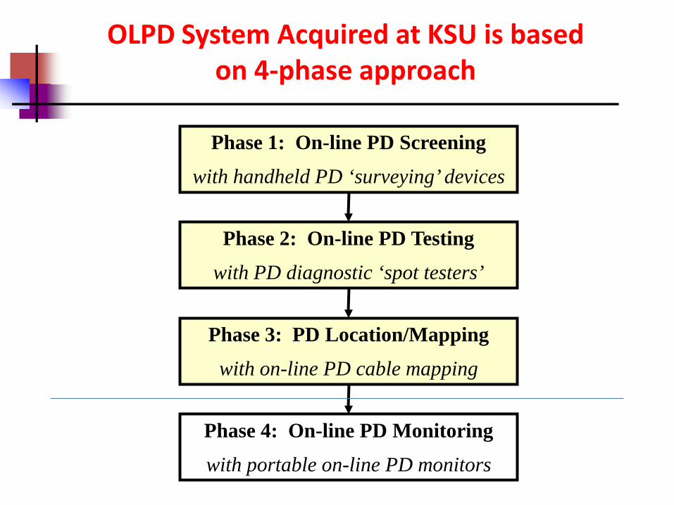
OLPD System Acquired at KSU is based on 4-phase approach

Phase 1: On-line PD Screening

with handheld PD ‘surveying’ devices

Phase 2: On-line PD Testing

with PD diagnostic ‘spot testers’

Phase 3: PD Location/Mapping

with on-line PD cable mapping

Phase 4: On-line PD Monitoring

with portable on-line PD monitors

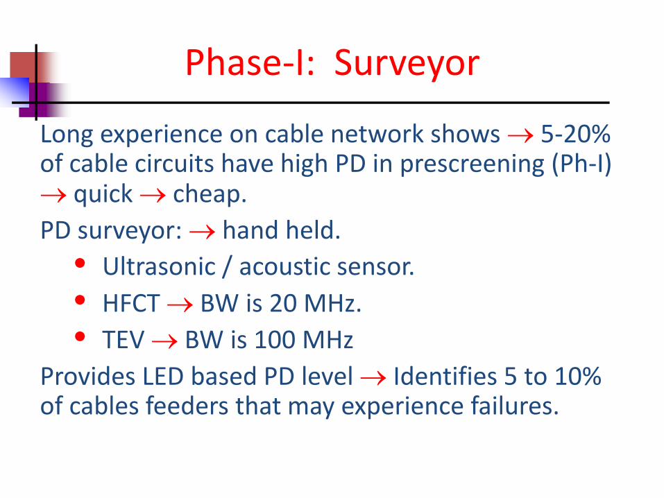
Long experience on cable network shows → 5-20% of cable circuits have high PD in prescreening (Ph-I) → quick → cheap. PD surveyor: → hand held.

• Ultrasonic / acoustic sensor. • HFCT → BW is 20 MHz. • TEV → BW is 100 MHz

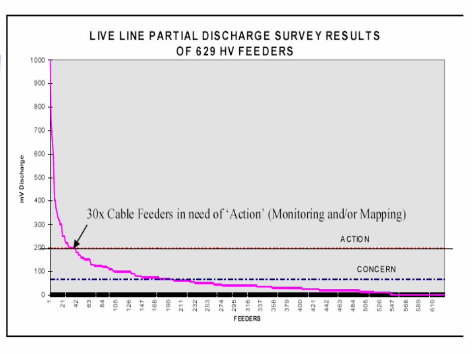
Provides LED based PD level → Identifies 5 to 10% of cables feeders that may experience failures.

Phase-I: Surveyor

Phase-II: ‘Longshot’ – Spot Tester

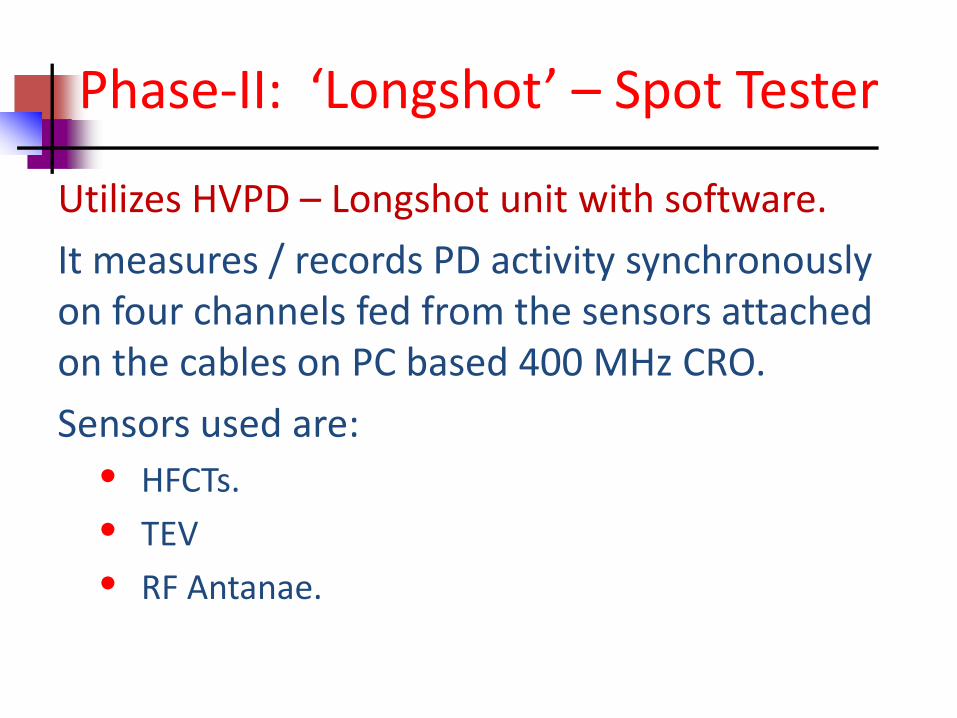
Utilizes HVPD – Longshot unit with software. It measures / records PD activity synchronously on four channels fed from the sensors attached on the cables on PC based 400 MHz CRO. Sensors used are:

• HFCTs. • TEV • RF Antanae.

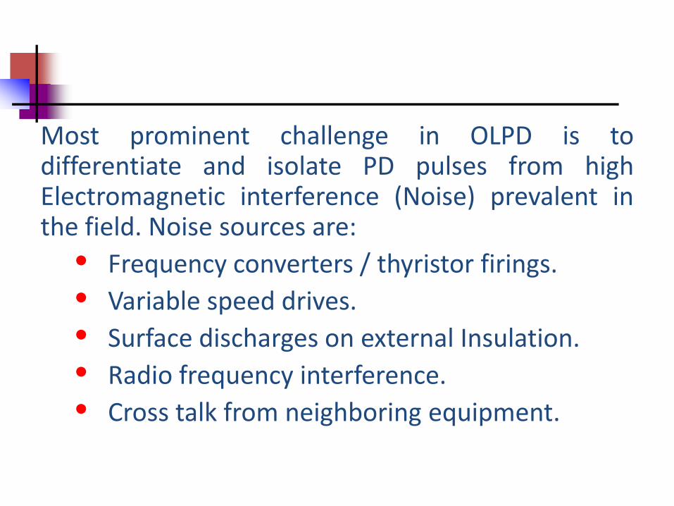
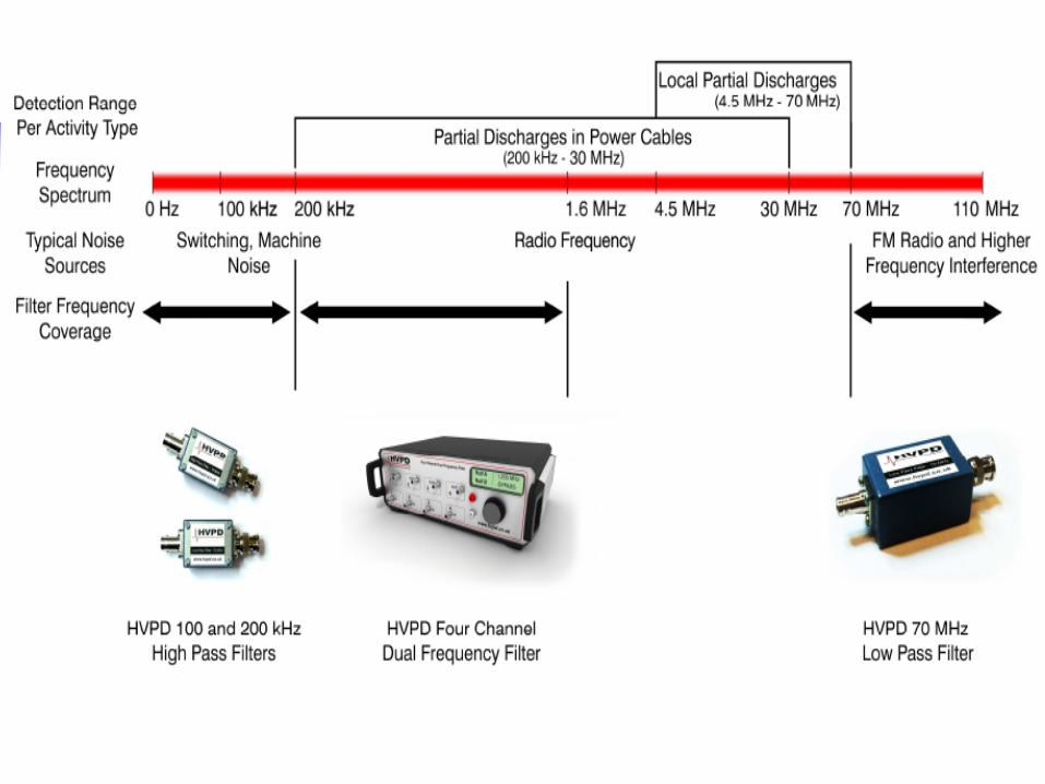
Most prominent challenge in OLPD is to differentiate and isolate PD pulses from high Electromagnetic interference (Noise) prevalent in the field. Noise sources are:

• Frequency converters / thyristor firings. • Variable speed drives. • Surface discharges on external Insulation. • Radio frequency interference. • Cross talk from neighboring equipment.

PD pulses undergo attenuation and dispersion during their travel in the cable and their rise time / fall time values change.

To isolate attenuated PD pulses from the noise pulses, state of the art filtering techniques are required.

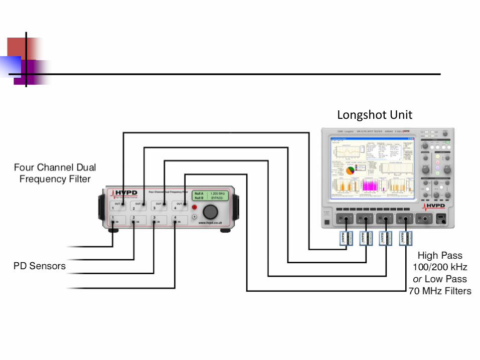
Longshot Unit

Long shot + set of filters, it is possible to: • Differentiate PD signals from noise. • Establish location of PD. • Device based on Windows PC + On board

LAN Port.

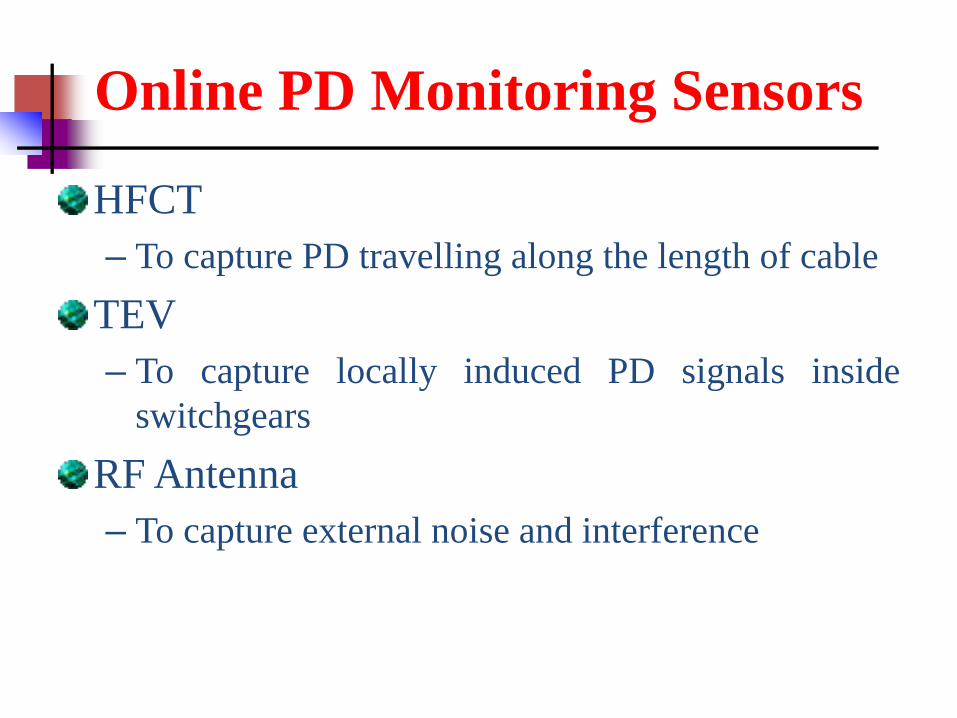
Online PD Monitoring Sensors

HFCT – To capture PD travelling along the length of cable

TEV – To capture locally induced PD signals inside

switchgears RF Antenna – To capture external noise and interference

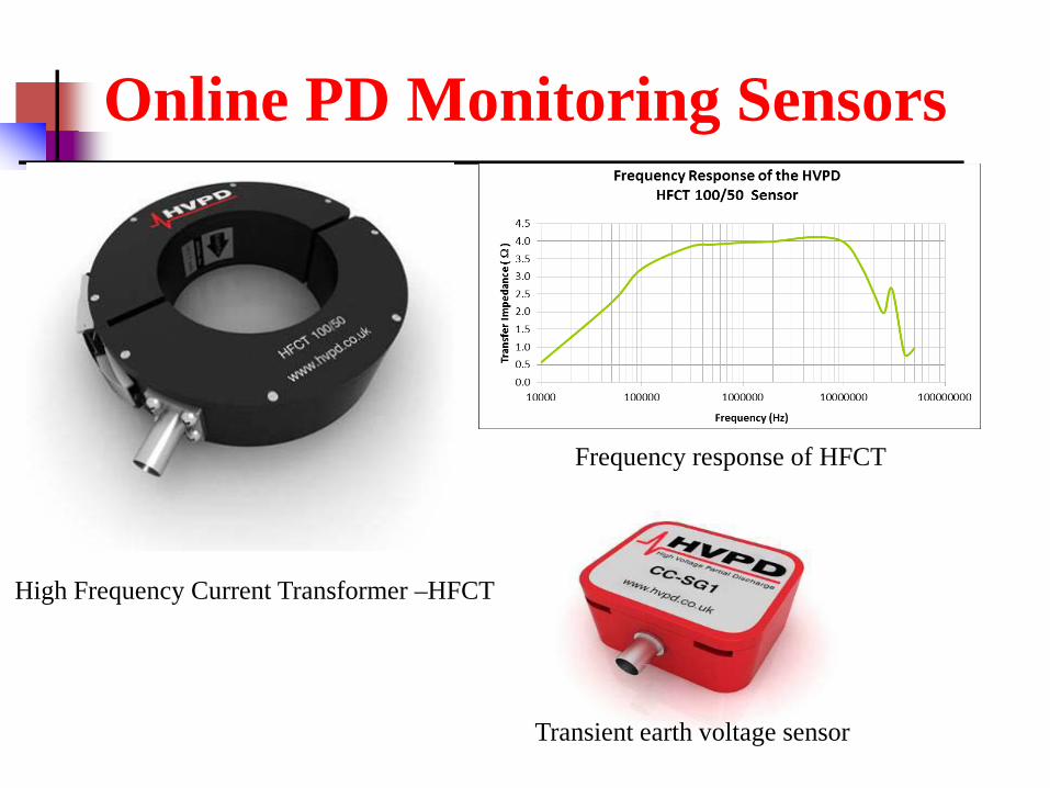
Online PD Monitoring Sensors

High Frequency Current Transformer –HFCT

Frequency response of HFCT

Transient earth voltage sensor

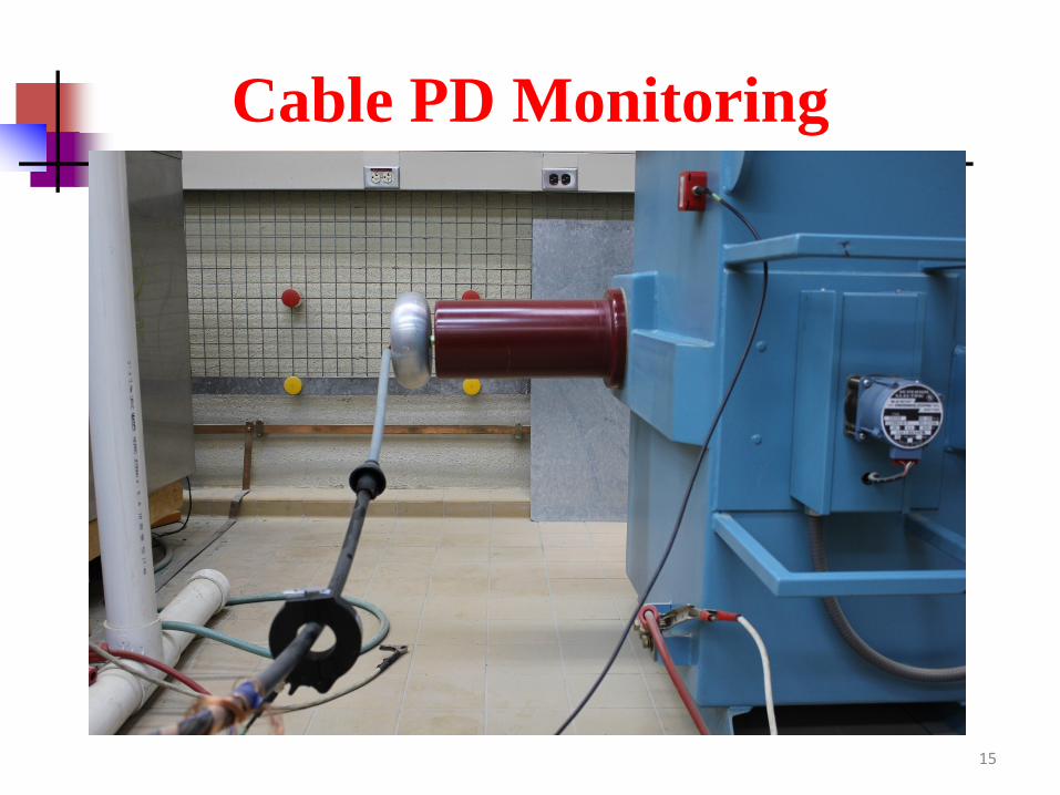
Cable PD Monitoring

15

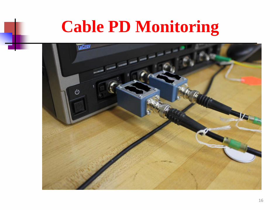
Cable PD Monitoring

16

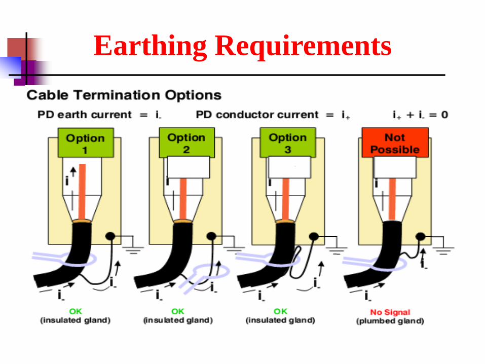
Earthing Requirements

There are two prerequisites for conducting a successful online PD measurements.

There must be independent access to either the earth-strap or the core of the cable at the switchgear/transformer. There must be an insulated gland between the cable earth and the switchgear earth.

Earthing Requirements

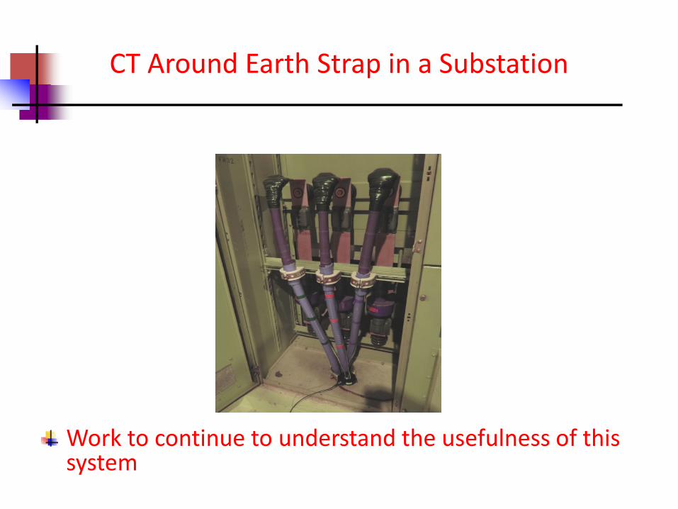
CT Around Earth Strap in a Substation

Work to continue to understand the usefulness of this system

Laboratory Experimental Setup

Long cable with proper terminations One end connected to HV transformer Other end open Toroid is used at the end to relief electric field stress around sharp edges of conductor. HFCT around core or earth TEV near the termination

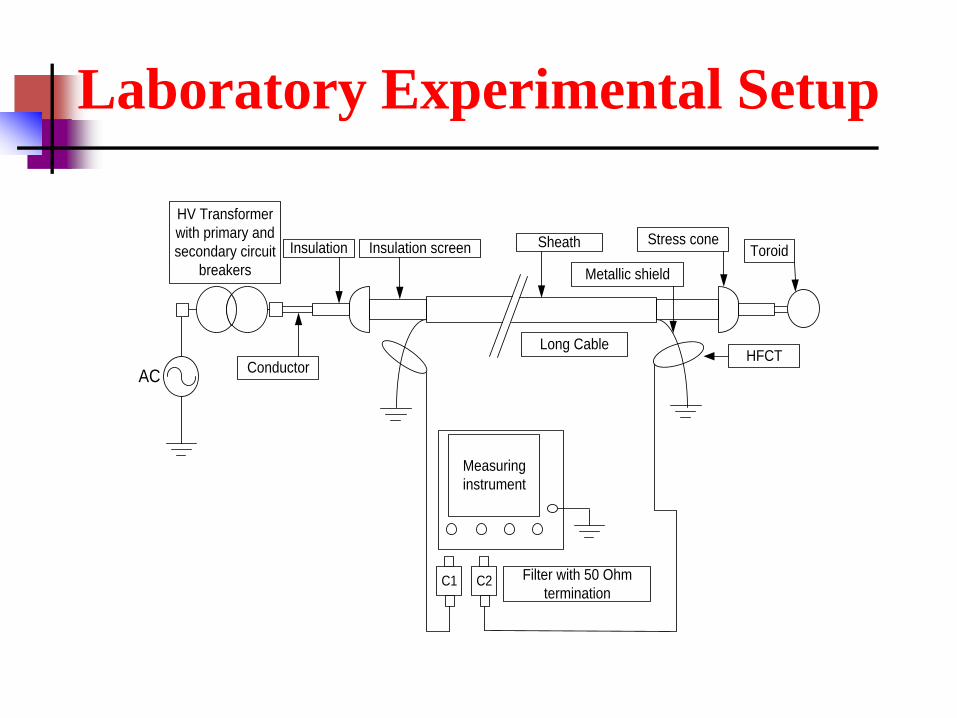
Laboratory Experimental Setup

Long Cable

HV Transformer with primary and secondary circuit

breakers

AC Conductor

Insulation Insulation screen

Metallic shield

Sheath Toroid

Measuring instrument

C1 C2 Filter with 50 Ohm termination

Stress cone

HFCT

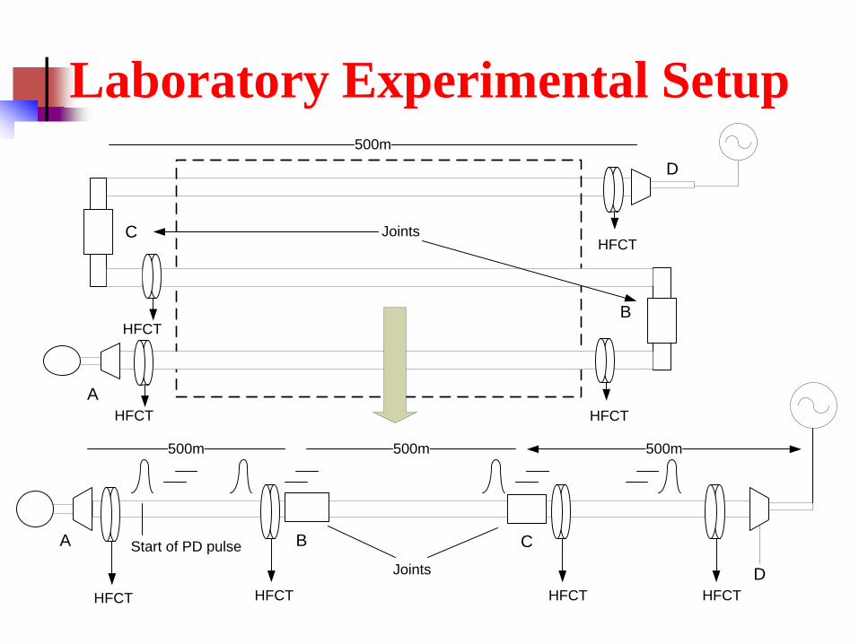
Laboratory Experimental Setup D

C

B

A

HFCT

HFCT

A

HFCTD

HFCT

B C

500m500m500m

JointsStart of PD pulse

500m

Joints

HFCT HFCT

HFCT

HFCT

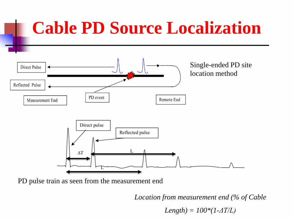
Cable PD Source Localization

Single-ended PD site location method

PD pulse train as seen from the measurement end

Location from measurement end (% of Cable

Length) = 100*(1-ΔT/L)

Cable PD Source Localization

Cable PD Source Localization

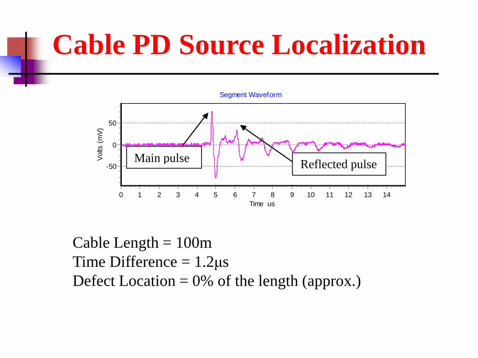
Segment Waveform

Time us14131211109876543210

Volts

(mV)

50

0

-50 Reflected pulse Main pulse

Cable Length = 100m Time Difference = 1.2μs Defect Location = 0% of the length (approx.)

Cable PD Source Localization

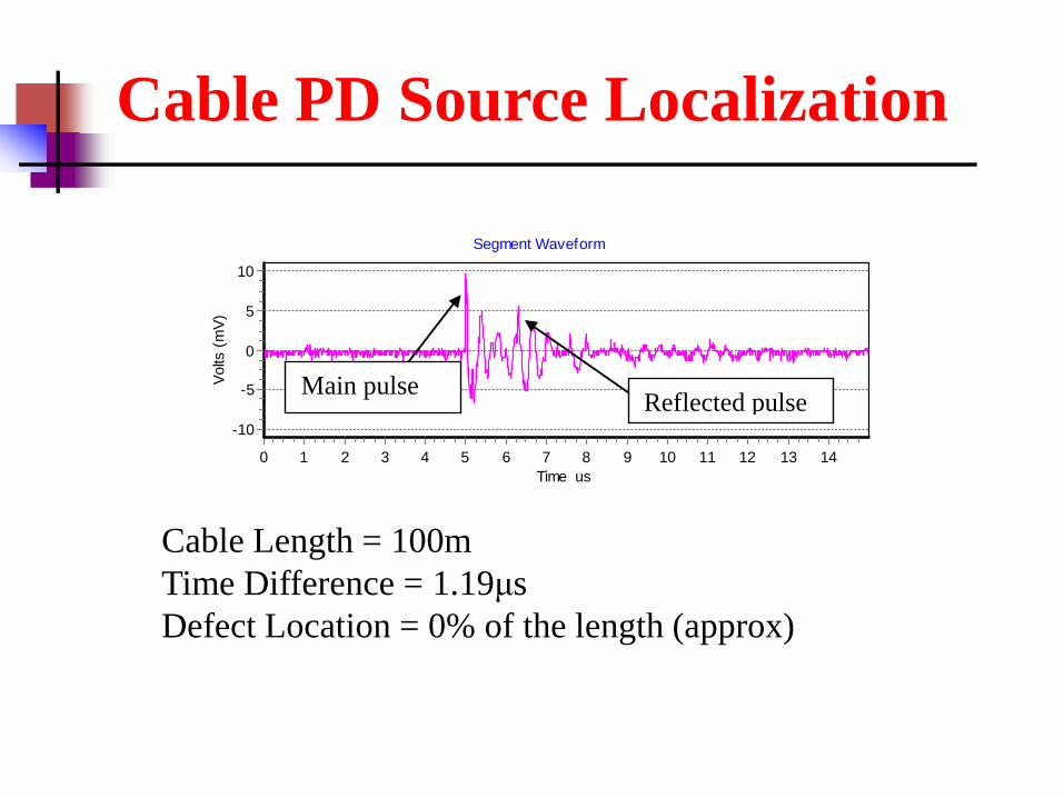
Segment Waveform

Time us14131211109876543210

Volts

(mV)

10

5

0

-5

-10

Main pulse Reflected pulse

Cable Length = 100m Time Difference = 1.19μs Defect Location = 0% of the length (approx)

Cable PD Source Localization

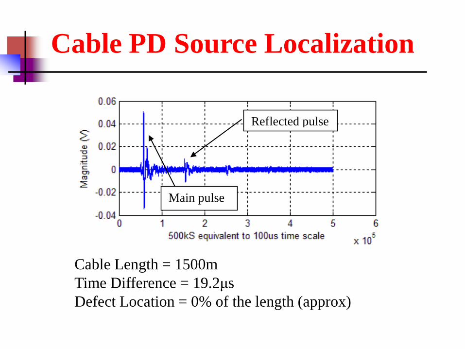
Main pulse

Reflected pulse

Cable Length = 1500m Time Difference = 19.2μs Defect Location = 0% of the length (approx)

Cable PD Source Localization

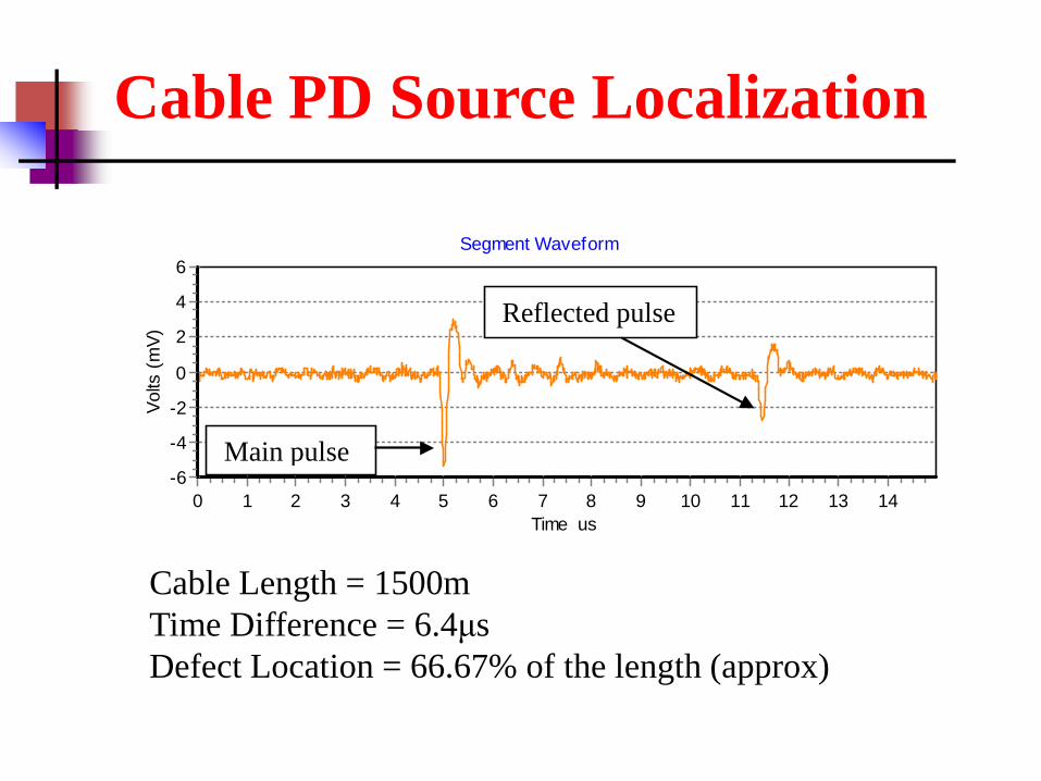
Segment Waveform

Time us14131211109876543210

Volts

(mV)

6

4

2

0

-2

-4

-6Main pulse

Reflected pulse

Cable Length = 1500m Time Difference = 6.4μs Defect Location = 66.67% of the length (approx)

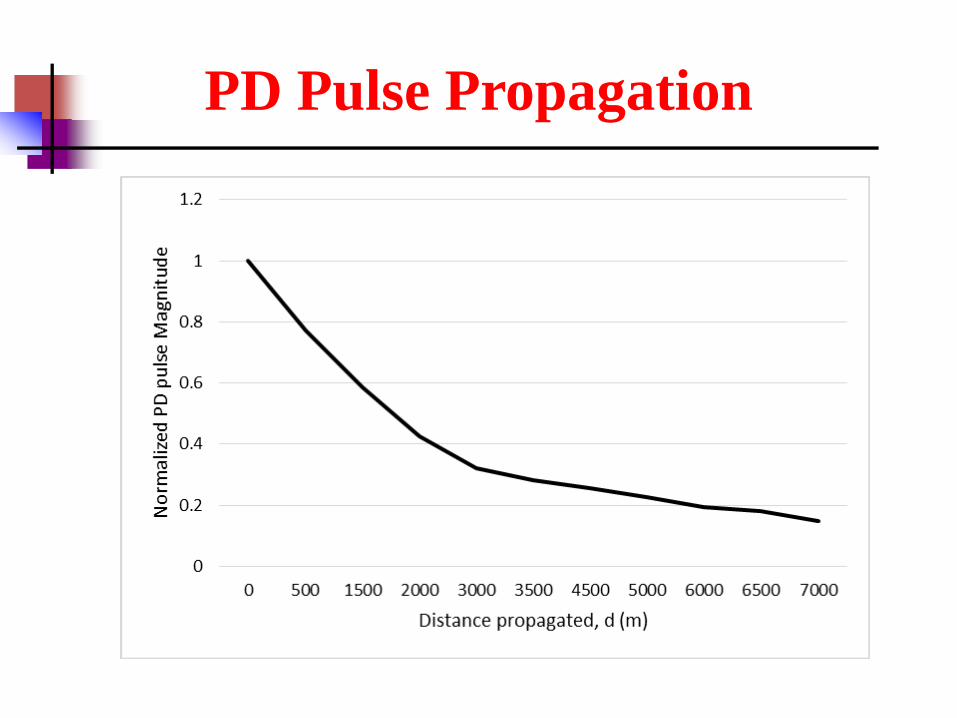
PD Pulse Propagation

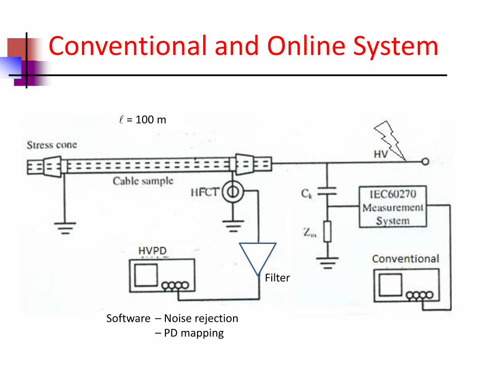
Conventional and Online System

= 100 m

Software – Noise rejection – PD mapping

Filter

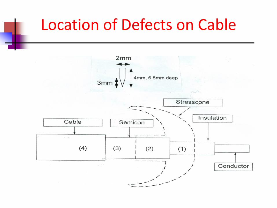
Location of Defects on Cable

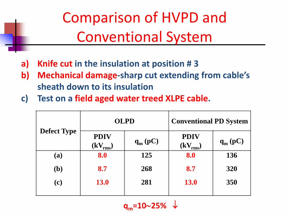
Comparison of HVPD and Conventional System

a) Knife cut in the insulation at position # 3 b) Mechanical damage-sharp cut extending from cable’s

sheath down to its insulation c) Test on a field aged water treed XLPE cable.

Defect Type

OLPD Conventional PD System

PDIV (kVrms)

qm (pC) PDIV (kVrms)

qm (pC)

(a)

(b)

(c)

8.0

8.7

13.0

125

268

281

8.0

8.7

13.0

136

320

350

qm=10∼25% ↓

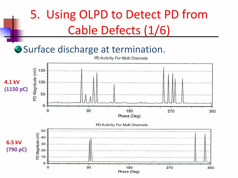
5. Using OLPD to Detect PD from Cable Defects (1/6)

Surface discharge at termination.

4.1 kV (1150 pC)

6.5 kV (790 pC)

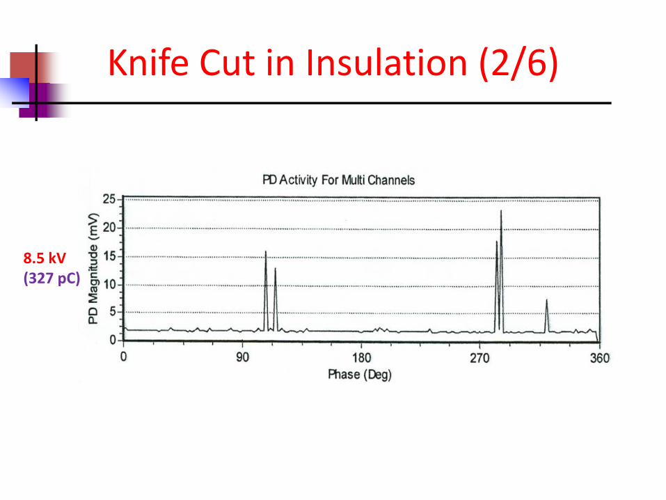
Knife Cut in Insulation (2/6)

8.5 kV (327 pC)

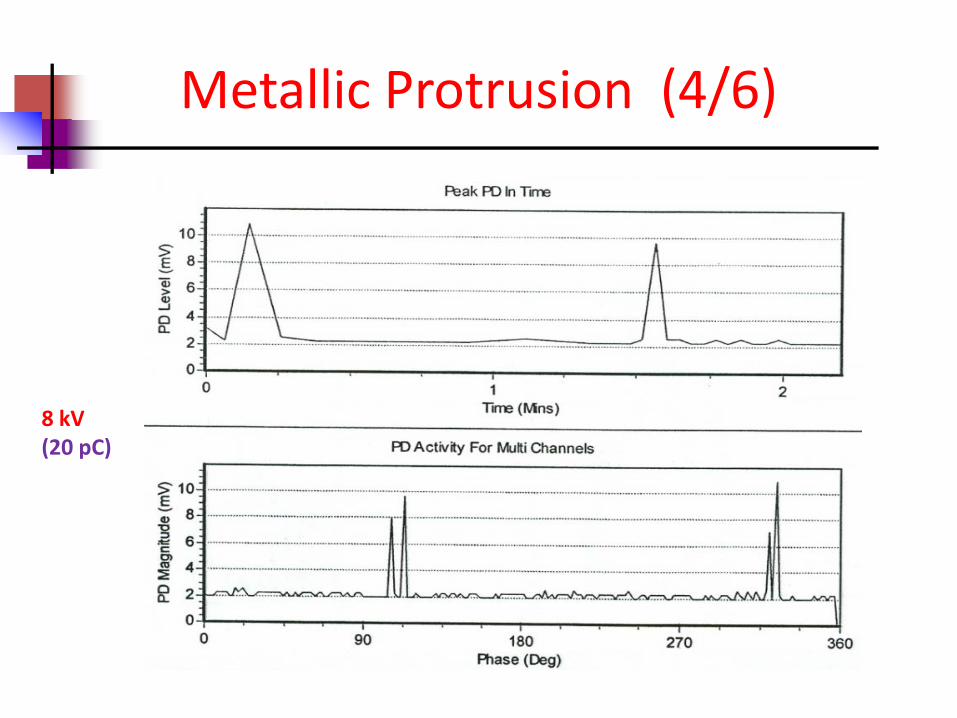
Metallic Protrusion (4/6)

8 kV (20 pC)

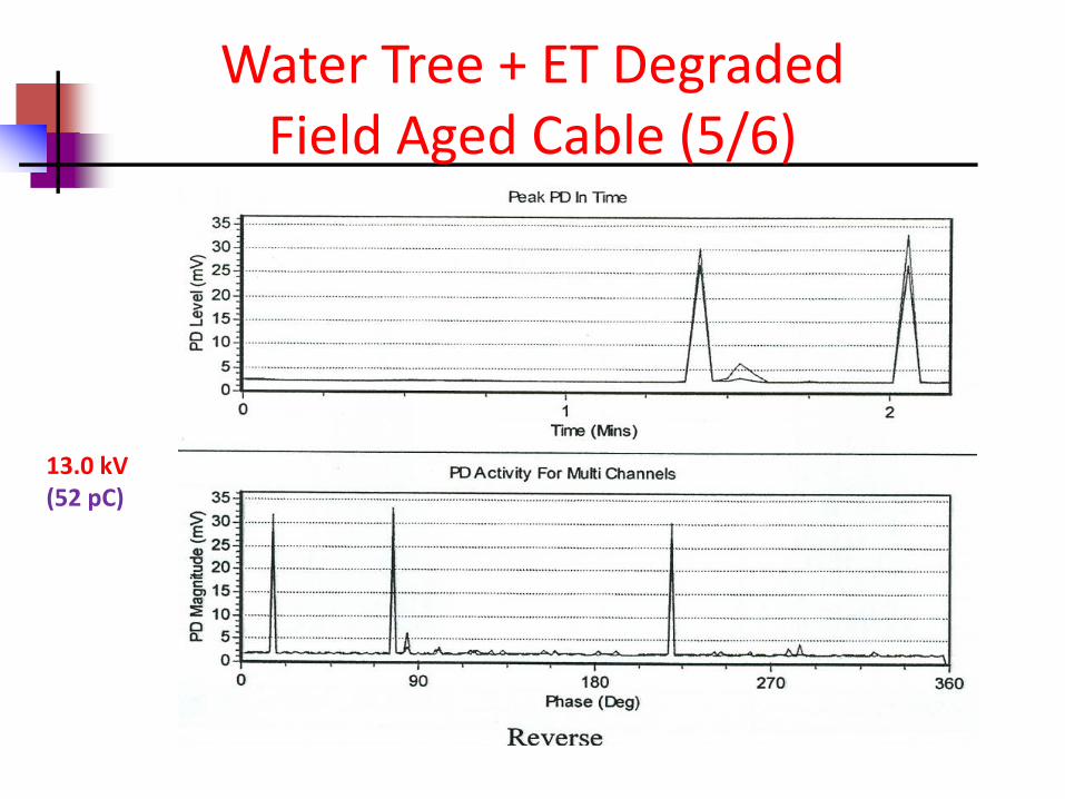
Water Tree + ET Degraded Field Aged Cable (5/6)

13.0 kV (52 pC)

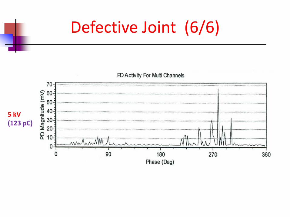
Defective Joint (6/6)

5 kV (123 pC)

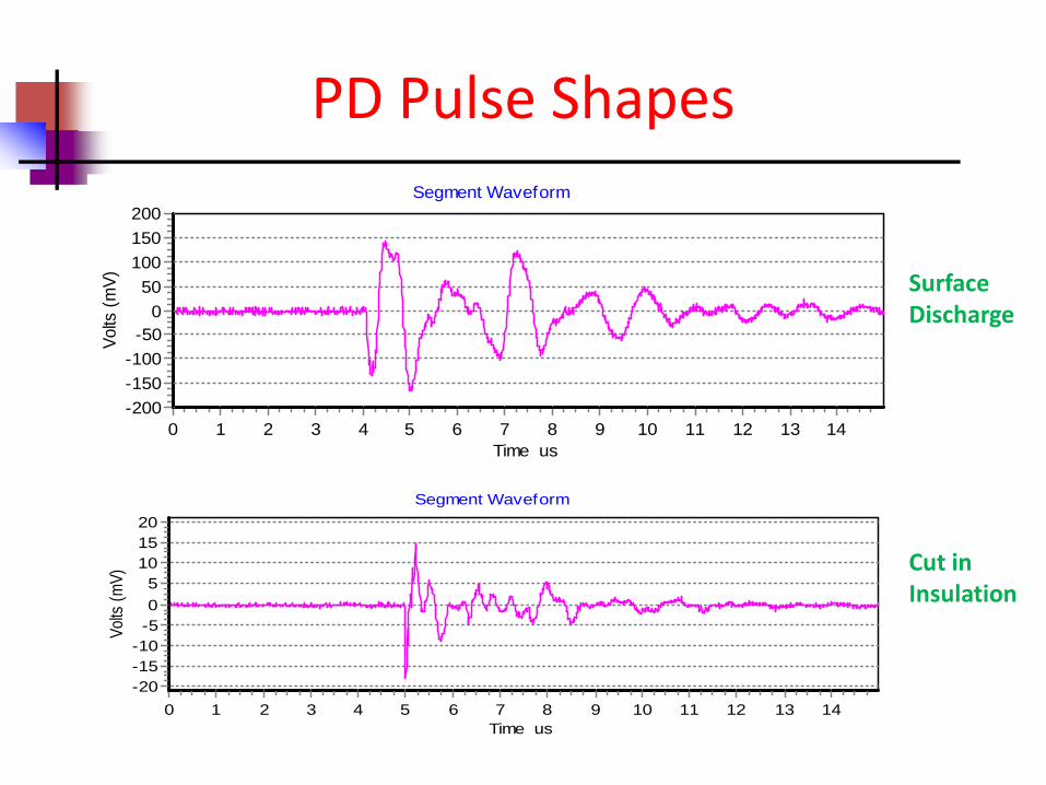
PD Pulse Shapes

Surface Discharge

Segment Waveform

Time us14131211109876543210

Volts

(mV)

200150100

500

-50-100-150-200

Segment Waveform

Time us14131211109876543210

Volts

(mV)

201510

50

-5-10-15-20

Cut in Insulation

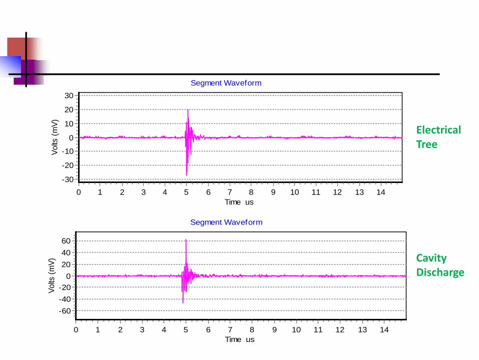
Electrical Tree

Cavity Discharge

Segment Waveform

Time us14131211109876543210

Volts

(mV)

604020

0-20-40-60

Segment Waveform

Time us14131211109876543210

Volts

(mV)

30

20

10

0

-10

-20

-30

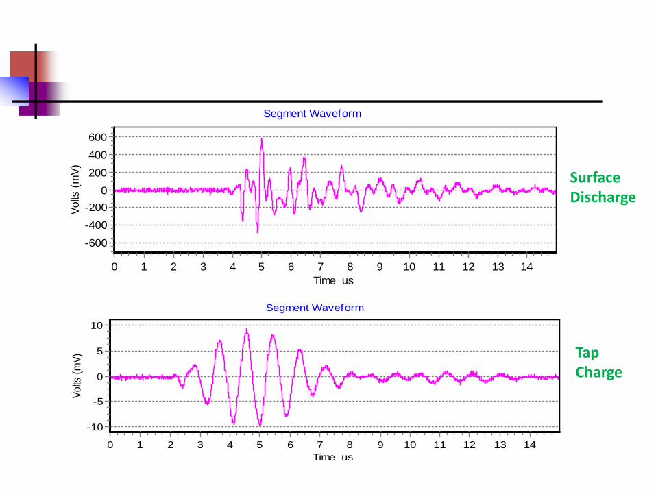
Surface Discharge

Tap Charge

Segment Waveform

Time us14131211109876543210

Volts

(mV)

600400200

0-200-400-600

Segment Waveform

Time us14131211109876543210

Volts

(mV)

10

5

0

-5

-10