on March 7, 2018 Stabilityofsubseapipelines...

rsta.royalsocietypublishing.org

ResearchCite this article: Draper S, An H, Cheng L,White DJ, Griffiths T. 2015 Stability of subseapipelines during large storms. Phil. Trans. R.Soc. A 373: 20140106.http://dx.doi.org/10.1098/rsta.2014.0106

One contribution of 12 to a Theme Issue‘Advances in fluid mechanics for offshoreengineering: a modelling perspective’.

Subject Areas:ocean engineering

Keywords:pipeline stability, scour, offshorehydrodynamics

Author for correspondence:Scott Drapere-mail: [email protected]

Stability of subsea pipelinesduring large stormsScott Draper1,2, Hongwei An2, Liang Cheng2,

David J. White3 and Terry Griffiths4

1Centre for Offshore Foundation Systems, 2School of Civil,Environmental and Mining Engineering, and 3Shell EMI Chair ofOffshore Engineering, University of Western Australia, 35 StirlingHwy, Crawley, Perth, WA 6009, Australia4Wood Group Kenny, Wood Group House, 432 Murray St., Perth,WA 6000, Australia

On-bottom stability design of subsea pipelinestransporting hydrocarbons is important to ensuresafety and reliability but is challenging to achievein the onerous metocean (meteorological andoceanographic) conditions typical of large storms(such as tropical cyclones, hurricanes or typhoons).This challenge is increased by the fact that industrydesign guidelines presently give no guidance onhow to incorporate the potential benefits of seabedmobility, which can lead to lowering and self-burialof the pipeline on a sandy seabed. In this paper,we demonstrate recent advances in experimentalmodelling of pipeline scour and present resultsinvestigating how pipeline stability can changein a large storm. An emphasis is placed on theinitial development of the storm, where scour isinevitable on an erodible bed as the storm velocitiesbuild up to peak conditions. During this initialdevelopment, we compare the rate at which peaknear-bed velocities increase in a large storm (typicallyless than 10−3 m s−2) to the rate at which a pipelinescours and subsequently lowers (which is dependentnot only on the storm velocities, but also on themechanism of lowering and the pipeline properties).We show that the relative magnitude of these ratesinfluences pipeline embedment during a storm andthe stability of the pipeline.

1. IntroductionThe lateral stability of subsea pipelines and cables inlarge storms is an important design requirement for oiland gas developments and is also of importance for data

2014 The Author(s) Published by the Royal Society. All rights reserved.

on May 26, 2018http://rsta.royalsocietypublishing.org/Downloaded from

http://crossmark.crossref.org/dialog/?doi=10.1098/rsta.2014.0106&domain=pdf&date_stamp=2014-12-15

mailto:[email protected]

http://rsta.royalsocietypublishing.org/

2

rsta.royalsocietypublishing.orgPhil.Trans.R.Soc.A373:20140106

.........................................................

communication infrastructure and marine renewable electricity networks. To ensure lateralstability two approaches are commonly employed in practice. Firstly, the pipeline or cable self-weight may be increased (known as primary stabilization) with the addition of, for example,a concrete coating in the case of pipelines. Secondly, additional means of stabilization may beadopted (known as secondary stabilization), which may include trenching, anchoring, placementof mattresses or overweight clamps and/or rock dumping. Presently, each of these approachesare known to provide reliable design solutions, but they come at a cost, with accounts suggestingthat stabilization comprises 30% of the cost of recent pipeline projects [1]. This is a substantialamount given that the total capital cost of pipelines typically exceeds US $4 million per kilometreof pipe [2].

Primary and secondary stabilization solutions are designed on the basis of conventionaldesign approaches, incorporating industry guidelines such as DNV-RP-F109 [3] and industry bestpractices (e.g. [4]). However, it is widely accepted that these design approaches are simplified andmay be overly conservative on a sandy seabed, because they do not account for any variationin pipeline embedment due to scour following the initial placement of the pipeline. This isdespite the fact that the same wave and current velocities that are evaluated to assess pipelinestability will almost always have the potential to mobilize sediment on a sandy seabed well beforethey can mobilize the pipeline [5]. A more correct stability analysis must therefore account forscour of sediment from beneath the pipeline and the potential for pipeline lowering, which willalter pipeline embedment and have a direct impact on hydrodynamic loading and lateral soilresistance. It is noted that previous work has incorporated changes to pipeline embedment intostability analysis (e.g. [6,7]), but this work has focused on changes in embedment due to cyclicloading of the pipeline as opposed to changes in embedment due to scour.

The detailed processes of pipeline scour and lowering have been described at length byFredsøe et al. [8] and Sumer & Fredsøe [9,10]. They are known to commence due to pre-existinggaps under the pipeline or when a scour hole initiates beneath a pipeline due to ‘piping’(e.g. [11,12]) or, for example, due to variations in sediment supply [13]. The scour hole then tendsto expand vertically beneath the pipe in a process known as tunnel erosion, which occurs at arate that is dependent on the near-seabed velocity, the pipeline geometry and the pipeline initialembedment [10,14]. The scour hole will also begin to extend along the pipeline at a rate that isdependent on these same parameters in addition to the three-dimensional geometry of the scourhole and the span shoulders [15–18].

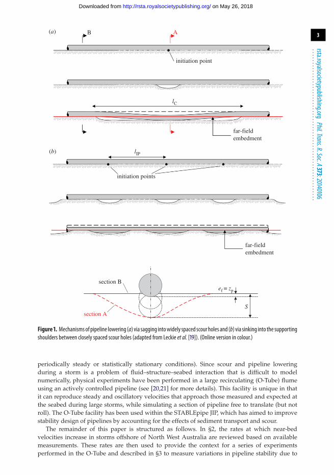
At some point, the scour hole(s) become sufficiently long that lowering of the pipeline occurs.In principle, two mechanisms can cause this lowering (figure 1). Firstly, if scour holes initiate atlocations that are widely spaced along the pipeline (relative to a length lC ∼ (100D × EI/w′)1/4,where D is the pipeline diameter, EI is the bending stiffness of the pipeline and w′ is thesubmerged weight per unit length), the pipeline can ‘sag’ into the hole [8]. Alternatively, if thescour holes are closely spaced (i.e. lIP < lC, where lIP is the spacing between initiation points ofscour along the pipeline), then the pipeline can ‘sink’ into the supporting soil between spanswhen these span shoulders become short [9]. Detailed analysis of pipeline field observations hasidentified both of these lowering mechanisms on the North West Shelf of Australia [19].

Incorporating scour and pipeline lowering into stability design requires that the cumulativeeffects of scour can be estimated for all velocities contributing to sediment mobility prior tothe time at which stability is to be analysed. In a large storm, this therefore requires that scourassociated with the storm velocities leading up to peak conditions is included in the analysis.This type of analysis leads to some general questions. Firstly, does the stability of a pipelineincrease during the initial stages of a storm due to scour? And secondly, if the stability of apipeline increases (continuously or eventually) with scour, can sufficient scour happen duringthe initial development of a storm to ensure stability at the peak? Or, put more simply, how doesthe rate of scour and pipeline lowering compare with the rate at which near-bed current and wavevelocities increase in a typical storm, so as to influence the stability of a pipeline?

The principal aims of this paper are to investigate aspects of these questions by buildingon previous literature that has focused mainly on scour in stationary velocities (i.e. steady,



3


.........................................................

initiation point

initiation points

section B

section A

far-fieldembedment

far-fieldembedment

(a)

(b)

AB

ef = zp

S

lIP

lC

Figure 1. Mechanismsof pipeline lowering (a) via sagging intowidely spaced scour holes and (b) via sinking into the supportingshoulders between closely spaced scour holes (adapted from Leckie et al. [19]). (Online version in colour.)

periodically steady or statistically stationary conditions). Since scour and pipeline loweringduring a storm is a problem of fluid–structure–seabed interaction that is difficult to modelnumerically, physical experiments have been performed in a large recirculating (O-Tube) flumeusing an actively controlled pipeline (see [20,21] for more details). This facility is unique in thatit can reproduce steady and oscillatory velocities that approach those measured and expected atthe seabed during large storms, while simulating a section of pipeline free to translate (but notroll). The O-Tube facility has been used within the STABLEpipe JIP, which has aimed to improvestability design of pipelines by accounting for the effects of sediment transport and scour.

The remainder of this paper is structured as follows. In §2, the rates at which near-bedvelocities increase in storms offshore of North West Australia are reviewed based on availablemeasurements. These rates are then used to provide the context for a series of experimentsperformed in the O-Tube and described in §3 to measure variations in pipeline stability due to



4


.........................................................

scour in the development stage of a storm. Detailed results and analysis of these experiments arepresented for both the mechanisms of sagging and sinking in §§4 and 5, respectively. Discussionof the results is given in §6.

2. Storm developmentIn many offshore locations around the world, extreme environmental loading conditions aredominated by rapidly rotating low-pressure weather systems called cyclones (also calledhurricanes in the North Atlantic and North East Pacific Oceans or typhoons in the North WestPacific Ocean). This is particularly true in North West Australia, where approximately four orfive cyclones occur during November to April each year [22]. These cyclones tend to generate inthe warmer waters of the Arafura and Timor Seas, before travelling a few thousand kilometresin a west to southwest direction over their lifetime [23]. The intensity of a cyclone (which can bedefined in terms of the maximum wind speed at the centre of the storm [24]) and the direction (ortrack) can change continuously during its lifetime.

In intense cyclones (i.e. category 4/5 or 5/5) offshore of North West Australia, significant waveheights can exceed 10–15 m, with the actual height being dependent on the central pressure in thecyclone, the geometry of the cyclone (often defined in terms of the radius to maximum winds)and the forward velocity of the cyclone [25]. In addition to increased waves, currents driven bythe pressure and wind forcing associated with a cyclone can reach values in excess of 2 m s−1

near the water surface [26]. This magnitude is a function of the intensity of the cyclone (throughthe pressure and wind forcing) and the storm track relative to the coastline and the underlyingbathymetry [23,27].

To provide some insight into the development of cyclonic storms, figure 2 reproduces surfacewave measurements and current measurements obtained in approximately 125 m water depth onthe North West Shelf of Australia at the North Rankin A (NRA) gas production platform operatedby Woodside. These measurements have been collated from a limited range of publications (citedin the figure captions). Cyclone storm tracks for each of these storm time series (obtained from[31]) are shown in figure 3 and summary statistics are given in table 1.

Figure 2 indicates that the significant wave heights at NRA tend to increase to a peak stormvalue over a period of approximately 12–36 h. During this period, the significant wave heightincreases continuously with a rate reaching approximately 0.3–1 m h−1 in the 3–6 h before peakconditions (table 1). Adopting linear wave theory, this indicates a rate of increase in the amplitudeof equivalent near-bed wave velocity of between 10−6 m s−2 and 10−5 m s−2 at NRA (whereequivalent near-bed wave velocity has been calculated using the approach outlined in [33];table 1).

The only current measurements in figure 2 are for Cyclone Orson. It can be seen that thesenear-surface currents oscillate prior to the arrival of peak wave conditions due to the semi-diurnaltide, but then accelerate at a maximum rate of around 0.25 m s−1 h−1 (or 6.9 × 10−5 m s−2) closeto peak storm conditions. In the case of Cyclone Orson accelerations of currents closer to the bedare less severe than those near the surface in figure 2. However, across a range of cyclones, theacceleration of near-bed currents is likely to be dependent on the amplification of both barotropicand baroclinic currents, and this makes them difficult to predict.

The ratio of steady current to wave velocity is important in assessing pipeline stability, becauseit has a strong influence on pipeline hydrodynamics and scour (for example, the equilibriumscour depth [10]). Although little comparative data are available, a general increase in the ratio ofcurrent to wave velocities is expected with increasing water depth.

In combination, the measurements in figure 2 and table 1 lead to several observations. Firstly,peak conditions occur after a finite ramp-up time, and so there is always likely to be sometime prior to peak storm conditions when the effects of scour can accumulate. Secondly, theacceleration associated with near-bed velocities for a particular location appears to be dependenton a number of factors, including not only the cyclone intensity but also the storm track. Forinstance, the present measurements show that fast ramp-up rates are experienced at NRA both



5


.........................................................

16(a)

(b)

(c)

(d )

12

8H

s (m

)H

s (m

)H

s (m

)H

s (m

)H

max

(m

)

4

0

1.5

1.0

0.5

0

curr

ent (

ms–1

)

16

12

8

4

0

16

12

8

4

0

16

12

8

4

0

16

12

8

4

00 12 24 36 48

time (h)

60 72 84 96

Figure 2. Time series of wave height and current (thin line only for case (a)) at NRA for five Tropical Cyclones: (a) TC Orson 1989,(b) TC Frank 1995, (c) TC Olivia 1996, (d) TC Tiffany 1998 and (e) TC Vance 1999. Data in (a) from Harper et al. [28], data in (c) fromBuchan et al. [29], data in (b,d,e) from Tron & Buchan [30]. (Online version in colour.)

in large storms (Orson) and in smaller storms (Tiffany) that track differently towards NRAbut at a similar forward speed. Thirdly, using NRA as a reference, the acceleration associatedwith the amplitude of near-bed wave velocity appears to be less than 10−5 m s−2 and theacceleration associated with surface current velocity is of the order of 10−4 m s−2 (note thatin the remainder of the paper the term ‘acceleration’ will be used to refer specifically to therate of increase of the amplitude in wave velocity or maximum combined wave and currentvelocity, not the instantaneous velocity). In an attempt to generalize this third observation, itis clear that accelerations below these values are expected for lower-intensity cyclones, or for



6


.........................................................

112

–12

–14

–16

–18

–20

–22

–24

–26

–28

–12

–14

–16

–18

–20

–22

–24

–26

–28

114 116 118 120 122 124 126 128

112 114 116 118 120 122 124 126 128

Australia

category 1–3

TC Frank TC Orson

TC Olivia

NRA Platform-

TC Tiffany

TC Vance

category 4

category 5

Figure 3. Cyclone tracks corresponding to storm time series given in figure 2. Circles represent location of cyclone every 6 h.(Online version in colour.)

cyclones tracking further from the design location. Conversely, for sites that are in much shallowerwater depth than NRA, the increase in significant wave heights shown in figure 2 could lead tolarger accelerations in wave velocity. However, it is unlikely they these accelerations will exceed10−3 m s−2 at the seabed unless the water depth is extremely shallow (i.e. less than 10 m) andthe rate of increase in wave height is significantly higher than that in figure 2 (i.e. around fivetimes higher than observed for Olivia). In the remainder of this paper, we will therefore adopt10−3 m s−2 as an upper estimate of the likely acceleration associated with significant wave velocityin a large storm. We will also adopt a similar acceleration (with less certainty) for near-bed currentvelocity and maximum combined near-bed wave and current velocity.

3. Experiments performed in O-Tube facilityA series of 12 experiments is reported in this paper. The first nine of these experiments investigatescour leading to the mechanism of sinking and the last three investigate scour leading to themechanism of sagging. The key difference between the sinking and sagging experiments is that inthe former the pipeline is actively load-controlled (using the approach outlined in [20]) to simulatethe self-weight of the pipe while allowing for horizontal and vertical translations. Consequently,it is possible to model the pipeline sinking into the seabed due to scour and to capture stabilitydirectly, by allowing the pipeline to translate due to any hydrodynamic forcing that exceeds theavailable soil resistance. By contrast, for the sagging experiments, the displacement of the pipelineis controlled so as to mimic vertical movement at the middle of a long span section of pipeline as



7


.........................................................

motor

ADV

ADV

camera

camera

Section A-Atop viewA

2000 mm

1000 mm

15 200 mm

1000 mmworking section 0

1000 mm1000 mm

pipe

sand

400

mm

1000

mm

00

A

pipe model

Figure 4. Large O-Tube, indicating location of pipeline and approximate location of camera.

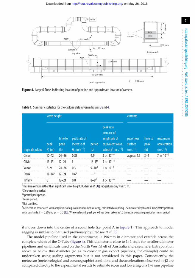
Table 1. Summary statistics for the cyclone data given in figures 3 and 4.

wave height currents

peak rateincrease of

time to peak rate of amplitude of peak near time to maximumpeak peak increase of period equivalent wave surface peak acceleration

tropical cyclone Hs (m) (h) Hs (m h−1) (s) velocityf (m s−2) (m s−1) (h) (m s−2)

Orson 10–12 24–36 0.85 9.1b 3 × 10−6 approx. 1.2 3–6 7 × 10−5. . . . . . . . . . . . . . . . . . . . . . . . . . . . . . . . . . . . . . . . . . . . . . . . . . . . . . . . . . . . . . . . . . . . . . . . . . . . . . . . . . . . . . . . . . . . . . . . . . . . . . . . . . . . . . . . . . . . . . . . . . . . . . . . . . . . . . . . . . . . . . . . . . . . . . . . . . . . . . . . . . . . . . . . . . . . . . . . . . . . . . . . . . . . . . . . . . . . . . . . . .

Olivia 12–13 12–24 1 12–13c 5 × 10−6 — — —. . . . . . . . . . . . . . . . . . . . . . . . . . . . . . . . . . . . . . . . . . . . . . . . . . . . . . . . . . . . . . . . . . . . . . . . . . . . . . . . . . . . . . . . . . . . . . . . . . . . . . . . . . . . . . . . . . . . . . . . . . . . . . . . . . . . . . . . . . . . . . . . . . . . . . . . . . . . . . . . . . . . . . . . . . . . . . . . . . . . . . . . . . . . . . . . . . . . . . . . . .

Vance 8–9 24–36 0.3 9–10d 1 × 10−6 — — —. . . . . . . . . . . . . . . . . . . . . . . . . . . . . . . . . . . . . . . . . . . . . . . . . . . . . . . . . . . . . . . . . . . . . . . . . . . . . . . . . . . . . . . . . . . . . . . . . . . . . . . . . . . . . . . . . . . . . . . . . . . . . . . . . . . . . . . . . . . . . . . . . . . . . . . . . . . . . . . . . . . . . . . . . . . . . . . . . . . . . . . . . . . . . . . . . . . . . . . . . .

Frank 12–14a 12–24 0.6a —e — — — —.. . . . . . . . . . . . . . . . . . . . . . . . . . . . . . . . . . . . . . . . . . . . . . . . . . . . . . . . . . . . . . . . . . . . . . . . . . . . . . . . . . . . . . . . . . . . . . . . . . . . . . . . . . . . . . . . . . . . . . . . . . . . . . . . . . . . . . . . . . . . . . . . . . . . . . . . . . . . . . . . . . . . . . . . . . . . . . . . . . . . . . . . . . . . . . . . . . . . . . . . .

Tiffany 8 12–24 0.8 8–9d 3 × 10−6 — — —. . . . . . . . . . . . . . . . . . . . . . . . . . . . . . . . . . . . . . . . . . . . . . . . . . . . . . . . . . . . . . . . . . . . . . . . . . . . . . . . . . . . . . . . . . . . . . . . . . . . . . . . . . . . . . . . . . . . . . . . . . . . . . . . . . . . . . . . . . . . . . . . . . . . . . . . . . . . . . . . . . . . . . . . . . . . . . . . . . . . . . . . . . . . . . . . . . . . . . . . . .aThis is maximum rather than significant wave height. Buchan et al. [32] suggest peak Hs was 7.3 m.bZero-crossing period.cSpectral peak period.dMean period.eNot specified.fAcceleration associated with amplitude of equivalent near-bed velocity, calculated assuming 125 m water depth and a JONSWAP spectrumwith constants B= 3.29 and γ = 3.3 [33]. Where relevant, peak period has been taken as 1.3 times zero-crossing period or mean period.

it moves down into the centre of a scour hole (i.e. point A in figure 1). This approach to modelsagging is similar to that used previously by Fredsøe et al. [8].

The model pipeline used in the experiments is 196 mm in diameter and extends across thecomplete width of the O-Tube (figure 4). This diameter is close to 1 : 1 scale for smaller-diameterpipelines and umbilicals used on the North West Shelf of Australia and elsewhere. Extrapolationabove or below this diameter (so as to consider gas export pipelines, for example) could beundertaken using scaling arguments but is not considered in this paper. Consequently, themetocean (meteorological and oceanographic) conditions and the accelerations observed in §2 arecompared directly to the experimental results to estimate scour and lowering of a 196 mm pipeline



8


.........................................................

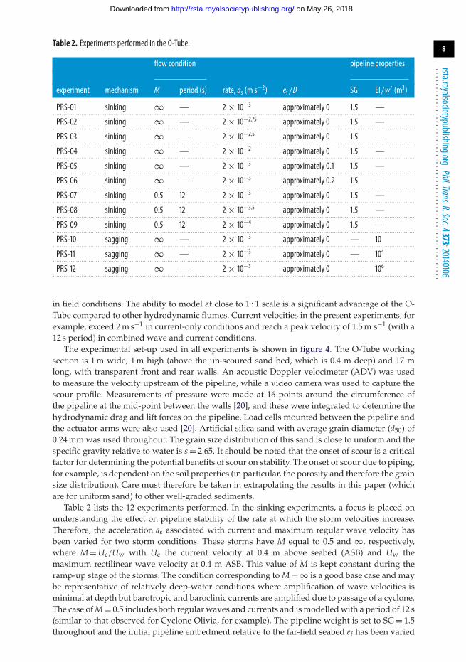
Table 2. Experiments performed in the O-Tube.

flow condition pipeline properties

experiment mechanism M period (s) rate, as (m s−2) ef/D SG EI/w′ (m3)

PRS-01 sinking ∞ — 2 × 10−3 approximately 0 1.5 —. . . . . . . . . . . . . . . . . . . . . . . . . . . . . . . . . . . . . . . . . . . . . . . . . . . . . . . . . . . . . . . . . . . . . . . . . . . . . . . . . . . . . . . . . . . . . . . . . . . . . . . . . . . . . . . . . . . . . . . . . . . . . . . . . . . . . . . . . . . . . . . . . . . . . . . . . . . . . . . . . . . . . . . . . . . . . . . . . . . . . . . . . . . . . . . . . . . . . . . . . .

PRS-02 sinking ∞ — 2 × 10−2.75 approximately 0 1.5 —. . . . . . . . . . . . . . . . . . . . . . . . . . . . . . . . . . . . . . . . . . . . . . . . . . . . . . . . . . . . . . . . . . . . . . . . . . . . . . . . . . . . . . . . . . . . . . . . . . . . . . . . . . . . . . . . . . . . . . . . . . . . . . . . . . . . . . . . . . . . . . . . . . . . . . . . . . . . . . . . . . . . . . . . . . . . . . . . . . . . . . . . . . . . . . . . . . . . . . . . . .

PRS-03 sinking ∞ — 2 × 10−2.5 approximately 0 1.5 —. . . . . . . . . . . . . . . . . . . . . . . . . . . . . . . . . . . . . . . . . . . . . . . . . . . . . . . . . . . . . . . . . . . . . . . . . . . . . . . . . . . . . . . . . . . . . . . . . . . . . . . . . . . . . . . . . . . . . . . . . . . . . . . . . . . . . . . . . . . . . . . . . . . . . . . . . . . . . . . . . . . . . . . . . . . . . . . . . . . . . . . . . . . . . . . . . . . . . . . . . .

PRS-04 sinking ∞ — 2 × 10−2 approximately 0 1.5 —. . . . . . . . . . . . . . . . . . . . . . . . . . . . . . . . . . . . . . . . . . . . . . . . . . . . . . . . . . . . . . . . . . . . . . . . . . . . . . . . . . . . . . . . . . . . . . . . . . . . . . . . . . . . . . . . . . . . . . . . . . . . . . . . . . . . . . . . . . . . . . . . . . . . . . . . . . . . . . . . . . . . . . . . . . . . . . . . . . . . . . . . . . . . . . . . . . . . . . . . . .

PRS-05 sinking ∞ — 2 × 10−3 approximately 0.1 1.5 —. . . . . . . . . . . . . . . . . . . . . . . . . . . . . . . . . . . . . . . . . . . . . . . . . . . . . . . . . . . . . . . . . . . . . . . . . . . . . . . . . . . . . . . . . . . . . . . . . . . . . . . . . . . . . . . . . . . . . . . . . . . . . . . . . . . . . . . . . . . . . . . . . . . . . . . . . . . . . . . . . . . . . . . . . . . . . . . . . . . . . . . . . . . . . . . . . . . . . . . . . .

PRS-06 sinking ∞ — 2 × 10−3 approximately 0.2 1.5 —. . . . . . . . . . . . . . . . . . . . . . . . . . . . . . . . . . . . . . . . . . . . . . . . . . . . . . . . . . . . . . . . . . . . . . . . . . . . . . . . . . . . . . . . . . . . . . . . . . . . . . . . . . . . . . . . . . . . . . . . . . . . . . . . . . . . . . . . . . . . . . . . . . . . . . . . . . . . . . . . . . . . . . . . . . . . . . . . . . . . . . . . . . . . . . . . . . . . . . . . . .

PRS-07 sinking 0.5 12 2 × 10−3 approximately 0 1.5 —. . . . . . . . . . . . . . . . . . . . . . . . . . . . . . . . . . . . . . . . . . . . . . . . . . . . . . . . . . . . . . . . . . . . . . . . . . . . . . . . . . . . . . . . . . . . . . . . . . . . . . . . . . . . . . . . . . . . . . . . . . . . . . . . . . . . . . . . . . . . . . . . . . . . . . . . . . . . . . . . . . . . . . . . . . . . . . . . . . . . . . . . . . . . . . . . . . . . . . . . . .

PRS-08 sinking 0.5 12 2 × 10−3.5 approximately 0 1.5 —. . . . . . . . . . . . . . . . . . . . . . . . . . . . . . . . . . . . . . . . . . . . . . . . . . . . . . . . . . . . . . . . . . . . . . . . . . . . . . . . . . . . . . . . . . . . . . . . . . . . . . . . . . . . . . . . . . . . . . . . . . . . . . . . . . . . . . . . . . . . . . . . . . . . . . . . . . . . . . . . . . . . . . . . . . . . . . . . . . . . . . . . . . . . . . . . . . . . . . . . . .

PRS-09 sinking 0.5 12 2 × 10−4 approximately 0 1.5 —. . . . . . . . . . . . . . . . . . . . . . . . . . . . . . . . . . . . . . . . . . . . . . . . . . . . . . . . . . . . . . . . . . . . . . . . . . . . . . . . . . . . . . . . . . . . . . . . . . . . . . . . . . . . . . . . . . . . . . . . . . . . . . . . . . . . . . . . . . . . . . . . . . . . . . . . . . . . . . . . . . . . . . . . . . . . . . . . . . . . . . . . . . . . . . . . . . . . . . . . . .

PRS-10 sagging ∞ — 2 × 10−3 approximately 0 — 10. . . . . . . . . . . . . . . . . . . . . . . . . . . . . . . . . . . . . . . . . . . . . . . . . . . . . . . . . . . . . . . . . . . . . . . . . . . . . . . . . . . . . . . . . . . . . . . . . . . . . . . . . . . . . . . . . . . . . . . . . . . . . . . . . . . . . . . . . . . . . . . . . . . . . . . . . . . . . . . . . . . . . . . . . . . . . . . . . . . . . . . . . . . . . . . . . . . . . . . . . .



in field conditions. The ability to model at close to 1 : 1 scale is a significant advantage of the O-Tube compared to other hydrodynamic flumes. Current velocities in the present experiments, forexample, exceed 2 m s−1 in current-only conditions and reach a peak velocity of 1.5 m s−1 (with a12 s period) in combined wave and current conditions.

The experimental set-up used in all experiments is shown in figure 4. The O-Tube workingsection is 1 m wide, 1 m high (above the un-scoured sand bed, which is 0.4 m deep) and 17 mlong, with transparent front and rear walls. An acoustic Doppler velocimeter (ADV) was usedto measure the velocity upstream of the pipeline, while a video camera was used to capture thescour profile. Measurements of pressure were made at 16 points around the circumference ofthe pipeline at the mid-point between the walls [20], and these were integrated to determine thehydrodynamic drag and lift forces on the pipeline. Load cells mounted between the pipeline andthe actuator arms were also used [20]. Artificial silica sand with average grain diameter (d50) of0.24 mm was used throughout. The grain size distribution of this sand is close to uniform and thespecific gravity relative to water is s = 2.65. It should be noted that the onset of scour is a criticalfactor for determining the potential benefits of scour on stability. The onset of scour due to piping,for example, is dependent on the soil properties (in particular, the porosity and therefore the grainsize distribution). Care must therefore be taken in extrapolating the results in this paper (whichare for uniform sand) to other well-graded sediments.

Table 2 lists the 12 experiments performed. In the sinking experiments, a focus is placed onunderstanding the effect on pipeline stability of the rate at which the storm velocities increase.Therefore, the acceleration as associated with current and maximum regular wave velocity hasbeen varied for two storm conditions. These storms have M equal to 0.5 and ∞, respectively,where M = Uc/Uw with Uc the current velocity at 0.4 m above seabed (ASB) and Uw themaximum rectilinear wave velocity at 0.4 m ASB. This value of M is kept constant during theramp-up stage of the storms. The condition corresponding to M = ∞ is a good base case and maybe representative of relatively deep-water conditions where amplification of wave velocities isminimal at depth but barotropic and baroclinic currents are amplified due to passage of a cyclone.The case of M = 0.5 includes both regular waves and currents and is modelled with a period of 12 s(similar to that observed for Cyclone Olivia, for example). The pipeline weight is set to SG = 1.5throughout and the initial pipeline embedment relative to the far-field seabed ef has been varied



9


.........................................................

(a) (b)

Figure 5. (a,b) Two snapshots of PRS-04. The pipeline moved laterally before experiencing significant scour. Dashed circleindicates initial location of the pipeline. Full circle identifies pipeline. Current is from the left. (Online version in colour.)

across three values (see figure 1 for definition of ef). Pipeline bending stiffness is not relevant inthe sinking experiments, because it is assumed that scour holes are sufficiently close (as requiredfor sinking) that curvature of the pipeline is minimal.

In the sagging experiments, the only variable that is altered is the simulated pipeline bendingstiffness to submerged weight ratio EI/w′. As will be explained later, this ratio determines thespeed at which the pipeline lowers into the centre of the scour hole. The focus of these experimentsis therefore to investigate the effect on pipeline stability of the rate at which the pipeline lowers.The value of EI/w′ = 104 m3 is typical of 200 mm diameter pipelines on the North West Shelf ofAustralia. The values of 101 m3 and 106 m3 are representative of a relatively ‘flexible’ and a ‘stiff’pipeline, respectively.

In addition to the experiments outlined in table 2, one supplementary experiment wasperformed to better explore sagging. This experiment is explained further in §5.

4. Pipeline sinkingIn experiments PRS-01 to PRS-09, the pipeline was placed on the seabed (at a particularembedment depth) and scour was observed at the edges of the pipeline as the current and wavevelocities increased. Following this, one of two outcomes was observed: (i) the storm velocitiesincreased rapidly and were sufficient to move the pipeline laterally (i.e. the pipeline was unstable)before the pipeline lowered significantly due to scour; or (ii) scour continued to develop andpropagated inwards towards the middle of the pipeline, which then began to sink vertically intothe seabed due to its own weight and remained laterally stable until it was completely buried.

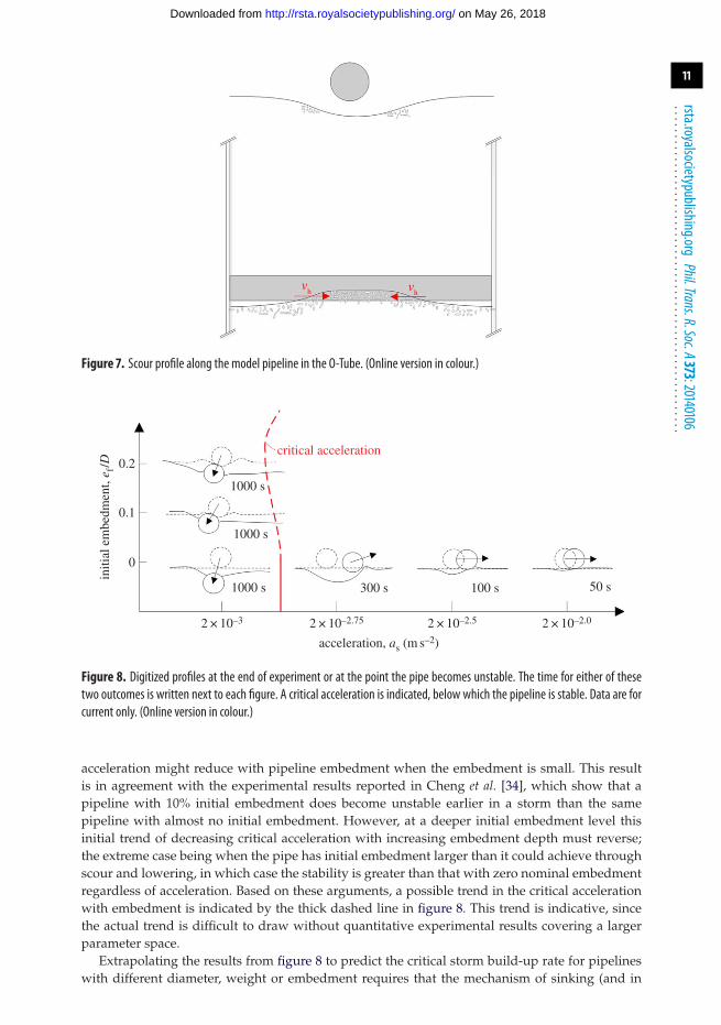
Figure 5 presents two snapshots of experiment PRS-04 consistent with the first of these twooutcomes. This pipeline became unstable after only 50 s of a current increasing from zero atan acceleration of 2 × 10−2 m s−2. Figure 6 presents snapshots for experiment PRS-01, whichmodelled the same pipeline but in a current accelerating at 2 × 10−3 m s−2, equivalent to theupper end of expected accelerations during a cyclone (as discussed in §2). In this experiment,the outcome was of the second type noted above, with the pipeline sinking by more than onediameter. The scour process observed in PRS-01 was similar to that drawn in figure 7, with scourdeveloping first at the sides of the pipeline in the O-Tube and then propagating at some velocityvh towards the middle of the pipeline. This pattern of scour was consistent across all experimentswhere scour development and pipeline lowering had time to occur. Preferential scour initiationat the ends of the pipeline occurred in each of these experiments primarily because of the localgeometry of the seal between the end of the model pipeline and the wall of the flume, whichresulted in a very small reduction in effective pipeline diameter at the walls of the flume.

In combination, the results in figures 5 and 6 demonstrate clearly how the rate at whichthe near-bed velocities increase can have a significant effect on the stability of the pipeline.A summary of the first six experiments in current-only conditions is presented in terms of theinitial and final digitized seabed profiles in figure 8. For an initial far-field embedment of zero, a‘critical’ acceleration exists between 2 × 10−3 and 2 × 10−2.75 m s−2. When the rate is lower than



10


.........................................................

(a) (b)

(e) ( f )

(c) (d )

Figure 6. (a–f ) Six snapshots of PRS-01 showing pipeline sinking into the seabed. Dashed circle indicates initial location of thepipeline. Full circle identifies pipeline. Current is from the left. (Online version in colour.)

this critical value, the pipeline experiences sufficient scour in the initial stages (less than 1 h) of thestorm to bury completely. By contrast, when the rate is higher than this critical value, the pipelinebecomes laterally unstable during the development of the storm.

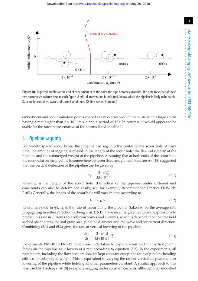
For experiments PRS-05 and PRS-06, the initial embedment of the pipeline was increasedartificially at the start of each experiment by translating the pipeline laterally across the seabedseveral times with amplitude of movement equal to one pipe diameter. This procedure could, forexample, represent the embedment increase due to pipe oscillations during the laying process, orwhen subjected to other cyclic loading (as noted in the Introduction). In both of these experiments,subsequent lowering of the pipeline due to scour was delayed compared with experiment PRS-01,which was conducted at the same acceleration but with no initial embedment. This delay isshown clearly in figure 9, which presents the vertical displacement of the pipeline in time andthe centroid of the pipeline as the pipeline lowers due to scour. The delay indicates that a highervelocity was required to initiate scour at the ends of the pipeline when the pipeline was morehighly embedded. This is consistent with the findings of Sumer et al. [12], who show that thecritical velocity to cause onset of scour due to piping increases with increased embedment.

In the present experiments, the pipeline was found to be stable in both PRS-05 and PRS-06;however, the delay in the onset of scour due to increased embedment suggests that the critical



11


.........................................................

vh v

h

Figure 7. Scour profile along the model pipeline in the O-Tube. (Online version in colour.)

0.2

0.1

2 × 10–3

1000 s 300 s 100 s 50 s

1000 s

1000 s

critical acceleration

2 × 10–2.75

acceleration, as (m s–2)

2 × 10–2.5 2 × 10–2.0

initi

al e

mbe

dmen

t, e f/

D

0

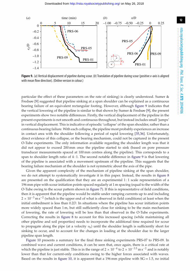
Figure 8. Digitized profiles at the end of experiment or at the point the pipe becomes unstable. The time for either of thesetwo outcomes is written next to each figure. A critical acceleration is indicated, below which the pipeline is stable. Data are forcurrent only. (Online version in colour.)

acceleration might reduce with pipeline embedment when the embedment is small. This resultis in agreement with the experimental results reported in Cheng et al. [34], which show that apipeline with 10% initial embedment does become unstable earlier in a storm than the samepipeline with almost no initial embedment. However, at a deeper initial embedment level thisinitial trend of decreasing critical acceleration with increasing embedment depth must reverse;the extreme case being when the pipe has initial embedment larger than it could achieve throughscour and lowering, in which case the stability is greater than that with zero nominal embedmentregardless of acceleration. Based on these arguments, a possible trend in the critical accelerationwith embedment is indicated by the thick dashed line in figure 8. This trend is indicative, sincethe actual trend is difficult to draw without quantitative experimental results covering a largerparameter space.

Extrapolating the results from figure 8 to predict the critical storm build-up rate for pipelineswith different diameter, weight or embedment requires that the mechanism of sinking (and in



12


.........................................................

0

(a) (b)

5 10 15 200

–0.2

–0.4

–0.6

e f/D

–0.8

–1.0

–1.2

–1.4

PRS-09PRS-01

PRS-01

PRS-05

PRS-05

PRS-06

PRS-09PRS-06x

ef

–1.00 –0.75 –0.50

x/Dtime (min)

–0.25 0 0.25

Figure 9. (a) Vertical displacement of pipeline during scour. (b) Translation of pipeline during scour (positive x-axis is alignedwith mean flow direction). (Online version in colour.)

particular the effect of these parameters on the rate of sinking) is clearly understood. Sumer &Fredsøe [9] suggested that pipeline sinking at a span shoulder can be explained as a continuousbearing failure of an equivalent rectangular footing. However, although figure 9 indicates thatthe vertical lowering of the pipeline is similar to that shown by Sumer & Fredsøe [9], the presentexperiments show two notable differences. Firstly, the vertical displacement of the pipeline in thepresent experiments is not smooth and continuous throughout, but instead includes small ‘jumps’in vertical displacement. This is indicative of episodic ‘collapse’ of the span shoulder, rather than acontinuous bearing failure. With each collapse, the pipeline most probably experiences an increasein contact area with the shoulder following a period of rapid lowering [35,36]. Unfortunately,direct evidence of this collapse, or the bearing mechanism, could not be captured in the presentO-Tube experiments. The only information available regarding the shoulder length was that itdid not appear to exceed 200 mm once the pipeline started to sink (based on pore pressuretransducer measurements spaced at 100 mm centres along the pipeline). This corresponds to aspan to shoulder length ratio of 4 : 1. The second notable difference in figure 9 is that loweringof the pipeline is associated with a movement upstream of the pipeline. This suggests that thebearing failure mechanism at the shoulder is not symmetric about the axis of the pipe.

Given the apparent complexity of the mechanism of pipeline sinking at the span shoulder,we do not attempt to systematically investigate it in this paper. Instead, the results in figure 8are presented on the qualification that they are an experimental 1 : 1 scale representation of a196 mm pipe with scour initiation points spaced regularly at 1 m spacing (equal to the width of theO-Tube owing to the scour pattern shown in figure 7). If this is representative of field conditions,then it is apparent that the pipeline would be stable under ramping currents up to and including2 × 10−3 m s−2 (which is the upper end of what is observed in field conditions) at least when theinitial embedment is less than 0.2D. In situations where the pipeline has scour initiation pointsmore widely spaced than 1 m, but still sufficiently close for sinking to be the main mechanismof lowering, the rate of lowering will be less than that observed in the O-Tube experiments.Correcting the results in figure 8 to account for this increased spacing (while maintaining allother pipeline and soil properties) needs to incorporate the additional time required for scourto propagate along the pipe (at a velocity vh) until the shoulder length is sufficiently short forsinking to occur, and to account for the changes in loading at the shoulder due to the largerpipeline span length.

Figure 10 presents a summary for the final three sinking experiments PRS-07 to PRS-09. Incombined wave and current conditions, it can be seen that, once again, there is a critical rate atwhich the pipeline is just stable. This is in the range of 2 × 10−4 to 2 × 10−3.5 m s−2 and is notablylower than that for current-only conditions owing to the higher forces associated with waves.Based on the results in figure 10, it is apparent that a 196 mm pipeline with SG = 1.5, no initial



13


.........................................................

2 × 10–4

6000 s

0

1000 s 600 s

2 × 10–3.5

acceleration, as (m s–2)

2 × 10–3

critical acceleration

initi

al e

mbe

dmen

t, e f/

D

Figure 10. Digitized profiles at the end of experiment or at the point the pipe becomes unstable. The time for either of thesetwo outcomes is written next to each figure. A critical acceleration is indicated, below which the pipeline is likely to be stable.Data are for combined wave and current conditions. (Online version in colour.)

embedment and scour initiation points spaced at 1 m centres would not be stable in a large stormhaving a rate higher than 2 × 10−4 m s−2 and a period of 12 s. In contrast, it would appear to bestable for the rates representative of the storms listed in table 1.

5. Pipeline saggingFor widely spaced scour holes, the pipeline can sag into the centre of the scour hole. At anytime, the amount of sagging is related to the length of the scour hole, the flexural rigidity of thepipeline and the submerged weight of the pipeline. Assuming that at both ends of the scour holethe constraint on the pipeline is somewhere between fixed and pinned, Fredsøe et al. [8] suggestedthat the vertical deflection of the pipeline can be given by

zp = 3384

w′l4sEI

, (5.1)

where ls is the length of the scour hole. (Deflection of the pipeline under different endconstraints can also be determined easily; see, for example, Recommended Practice DNV-RP-F105.) Generally, the length of the scour hole will vary in time according to

ls = 2vh × t, (5.2)

where, as noted in §4, vh is the rate of scour along the pipeline (taken to be the average ratepropagating in either direction). Cheng et al. [16,17] have recently given empirical expressions topredict this rate in currents and collinear waves and currents, which is dependent on the free fieldseabed shear stress, the soil grain size, pipeline diameter and the wave and/or current direction.Combining (5.1) and (5.2) gives the rate of vertical lowering of the pipeline

dzp

dt= 3

384w′

EIddt

{l4s }. (5.3)

Experiments PRS-10 to PRS-12 have been undertaken to explore scour and the hydrodynamicforces on the pipeline as it lowers at a rate according to equation (5.3). In the experiments, allparameters, including the flow acceleration, are kept constant except the ratio of pipeline bendingstiffness to submerged weight. This is equivalent to varying the rate of vertical displacement orlowering of the pipeline while holding all other parameters constant. A similar approach to thiswas used by Fredsøe et al. [8] to explore sagging under constant currents, although they modelled



14


.........................................................

0 10 20 30

A B C D

40 50 60 70 80 90 100 110 120

0 10 20

(a)

(b)

(c)

(d )

30 40 50 60 70 80 90 100 110 120

0 10 20 30 40 50 60 70 80 90 100 110 120

00

0.20.40.60.8

velo

city

(m

s–1)

1.01.2

1.21.00.80.60.40.2

1.41.21.00.80.60.40.2

0

1.4

0.58

1.06

1.28

1.2

S/D

, zp/

DS/

D, z

p/D

S/D

, zp/

D

1.00.80.60.40.2

0

0

1.4

1.4

10 20 30 40 50 60time (min)

70 80 90 100 110 120

Figure 11. Variation in scour depth and pipeline position with time. (a) PRS-10, (b) PRS-11 and (c) PRS-12. Solid dark line isthe location of the bottom of the pipeline, zp; circles are measured scour hole depth beneath the pipe; and dashed line isprediction from equation (5.6). (Online version in colour.)

a pipeline that dropped at a fixed rate. Using the model pipe in the O-Tube, it is relatively easyto adopt the more appropriate rate due to equation (5.3), which varies in time due to scour alongthe pipeline and the nonlinear relationship between vertical deflection and span length.

Figure 11 presents the experimental results for PRS-10 to PRS-12, giving the calculated verticaldisplacement of the pipeline (worked out using vh from [16] and equation (5.3)) and the scour holedepth as a function of time. The experimental velocity time series is also shown. The point in timewhen the vertical displacement of the pipeline matches the scour hole depth signifies when thepipeline has ‘touched down’ into the scour hole. At this point (identified as a spike in the vertical



15


.........................................................

(a)

(b)

(c)

Figure 12. Variation in scour profile as pipeline sags into scour hole. (a) PRS-10, (b) PRS-11 and (c) PRS-12. Current is from theleft. (Online version in colour.)

force reading via the load cells), no further vertical movement of the pipeline was simulated in theexperiment. In all three experiments, backfilling of the scour hole through sediment depositionthen commenced.

With respect to figure 11, it is clear that the final burial depth differs significantly across theexperiments. The most flexible pipeline drops fastest into the scour hole, but only reaches a depthof 0.58D. In contrast the stiff pipeline drops later and over a longer period of time, leading to afinal depth of 1.28D. Consequently, for the experiments considered herein, the potential changesto stability as a result of sagging are experienced faster for the flexible pipeline, but the extentof lowering and the potential for greater long-term stability are larger for the stiffer pipelineprovided it does not become unstable during the lowering process.

The reason for the difference in final lowered depth across the three experiments is dueto the fact that the vertical position of the pipeline has an effect on scour locally beneath thepipeline. This interaction is clear in figure 12 which presents the scour profile around the pipelineas it moves vertically into the scour hole; as the pipeline drops (but has not yet touched thebottom of the hole), the scour hole increases in depth and the side slopes become steeper andmore symmetric. This increase in scour hole depth does, however, take a finite time to occur.Consequently, the stiffer pipeline, which drops more slowly into the hole and allows sufficienttime for the additional scour to develop, can lower to a greater depth.

In the sinking experiments (discussed in §4), load control of the pipeline allowed stabilityof the pipeline to be observed directly, since translations of the pipeline were permitted duringtesting. By contrast, for the sagging experiments, changes to stability can be partially interpretedthrough the influence of sagging on the hydrodynamic forces experienced by the pipeline. Toexplore this influence, figure 13 presents the lift and drag coefficients for experiments PRS-10 and



16


.........................................................

1.0(a)

(b)

Jensen et al. [37]

Zhao & Cheng [38]

PRS-10

0 0.2 0.4 0.6S/D

CD

CL

0.8 1.0 1.2 1.4

PRS-11

PRS-11

PRS-10

sagging sagging

sagging sagging

0.8

0.6

0.4

0.2

0

–0.2

–0.4

–0.6

–0.8

–1.0

1.8

1.6

1.4

1.2

1.0

0.8

0.6

0.4

0.2

0

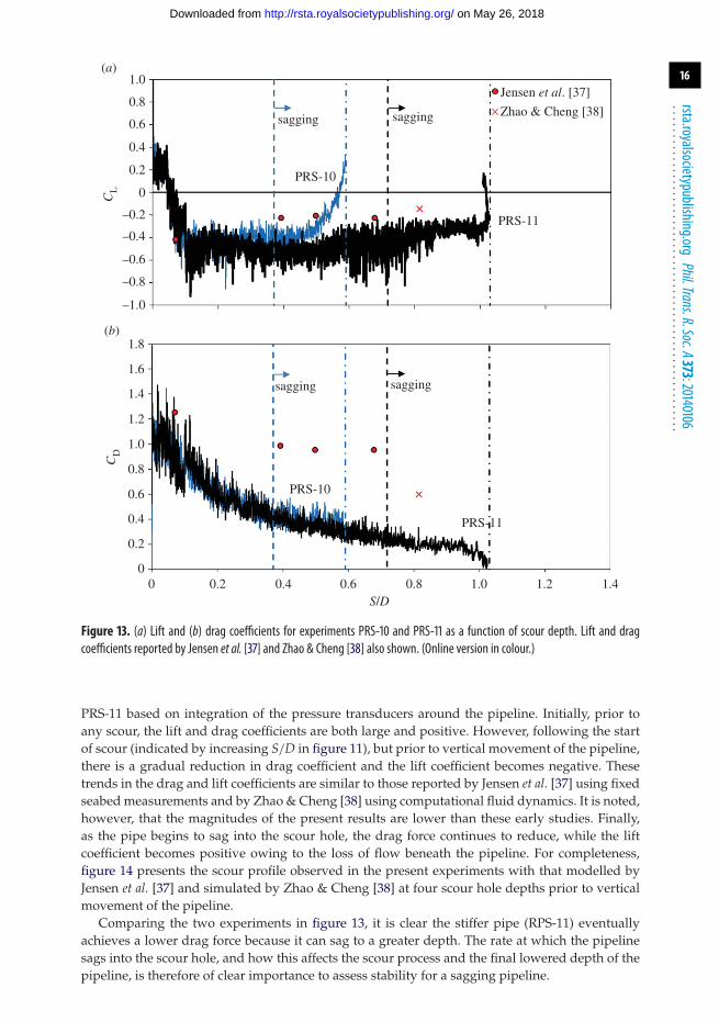
Figure 13. (a) Lift and (b) drag coefficients for experiments PRS-10 and PRS-11 as a function of scour depth. Lift and dragcoefficients reported by Jensen et al. [37] and Zhao & Cheng [38] also shown. (Online version in colour.)

PRS-11 based on integration of the pressure transducers around the pipeline. Initially, prior toany scour, the lift and drag coefficients are both large and positive. However, following the startof scour (indicated by increasing S/D in figure 11), but prior to vertical movement of the pipeline,there is a gradual reduction in drag coefficient and the lift coefficient becomes negative. Thesetrends in the drag and lift coefficients are similar to those reported by Jensen et al. [37] using fixedseabed measurements and by Zhao & Cheng [38] using computational fluid dynamics. It is noted,however, that the magnitudes of the present results are lower than these early studies. Finally,as the pipe begins to sag into the scour hole, the drag force continues to reduce, while the liftcoefficient becomes positive owing to the loss of flow beneath the pipeline. For completeness,figure 14 presents the scour profile observed in the present experiments with that modelled byJensen et al. [37] and simulated by Zhao & Cheng [38] at four scour hole depths prior to verticalmovement of the pipeline.

Comparing the two experiments in figure 13, it is clear the stiffer pipe (RPS-11) eventuallyachieves a lower drag force because it can sag to a greater depth. The rate at which the pipelinesags into the scour hole, and how this affects the scour process and the final lowered depth of thepipeline, is therefore of clear importance to assess stability for a sagging pipeline.



17


.........................................................

(a)

(b)

(c)

(e)

(d )

Figure 14. Profiles during the initial phase of scour (prior to pipeline movement). Dashed lines are digitized profiles fromexperiment PRS-11. Solid lines in (a–d) are from Jensen et al. [37] profiles II–V. Solid line in (e) is from Zhao & Cheng [38].Current is from the left.

To better quantify how the rate at which the pipeline sags alters the scour process, asupplementary experiment was performed in which the pipeline was held fixed above theseabed with a far-field embedment of zero. Scour was then allowed to develop until apparentequilibrium conditions were reached at a steady current velocity. Following this, the pipelinewas then lowered in discrete steps to vertical positions of zp/D = 0.2, 0.33, 0.46, 0.58, 0.71 and0.84. For each position, scour was allowed to develop until the scour depth appeared to reach aconstant value over a period between 1 and 5 min (it should be noted that only this short timeperiod was considered since waiting for longer, as could be appropriate for a pipeline much stifferthan any considered herein, could result eventually in backfill and a reduction in scour depth forlarger zp). Live bed scour was observed at all times. Figure 15 summarizes the results from thissupplementary experiment in terms of the scour hole depth. Each vertical dashed line indicateswhen the pipeline was lowered.

Two quantities are of interest in figure 15: (i) the evolution in apparent equilibrium scour depthSeq and (ii) the rate of scour with vertical movement of the pipeline. The first of these quantitiesclearly increases as the pipe moves downwards. This increase in depth, relative to the depth for



18


.........................................................

1.4

1.2

1.0

0.8

0.6

0.4

0.2

0 20 40 60 80 100

S/D

time (min)120 140 160 180 200

Figure 15. Developmentof scourholedepth for variouspipelinepositionsgivenby zp/D= 0, 0.2, 0.33, 0.46, 0.58, 0.71 and0.84.Measurements are circle markers. Vertical dashed lines separate intervals where the pipeline had a different vertical position.Solid line is fit based on equation (5.4). (Online version in colour.)

zp = 0, is shown to agree very well in figure 16 with the trend suggested by Sumer & Fredsøe[10] based on results from Hansen et al. [39]. To investigate the second quantity, the followingexpression has been fitted to each interval of the data in figure 15:

S(t) = Seq

(1 − exp

(− t − t0

T

)), (5.4)

where T defines a time scale of scour and t0 can be interpreted as an ‘offset’ in time required toensure that (5.4) agrees with the measured scour depth at the start of an interval after the pipelinehas been lowered. The form of (5.4) when t0 = 0 is the same as that introduced by Fredsøe et al. [40]to describe the scour hole development in steady currents for a pipeline with zp = 0. Adequatefitting of (5.4) using the equilibrium scour depths in figure 16 was achieved (figure 15) whenusing a single value of T = 350 s. For the first interval of zp/D = 0, this result is slightly lower thana value of 540 s calculated according to the empirical formula suggested by Fredsøe et al. [40] forthe sediment used in the experiment, the pipe diameter and the flow velocity.

The reasonable fit between (5.4) and the measurements in the supplementary experimentsuggests that the scour development observed in figure 11 might be well predicted for anypipeline vertical position using equation (5.4). Pursuing this approach, the rate of change in scourhole depth for a sagging pipeline may be predicted according to

dS′

dt=

S′eq(z′

p) − S′

T, (5.5)

where S′ = S/D and z′p = zp/D.

Using the vertical pipeline position z′p, equation (5.5) has been used to back-calculate the

changes in scour depth with time in figure 11 according to

S′(t) =∫ t

0

(S′

eq(z′p) − S′

T

)dt, (5.6)

where the equilibrium scour depth has been estimated according to the expression indicated bythe dashed line shown in figure 16:

S′eq = 0.86 exp(0.6z′

p). (5.7)

It should be noted that this expression is likely to have some upper limit of validity for largevalues of z′

p, although we are not able to state this limit based on the experiments presentedherein. The time scale has been assumed to be independent of pipe position, based on the results



19


.........................................................

2.0

1.8

1.6

1.4

1.2

1.0

0.8

0.6

0.4

0.2

0 0.2 0.4 0.6zp/D

S eq/D

Seq

zp

0.8 1.0 1.2

Figure 16. Variation in equilibrium scour depth as a function of pipeline far-field embedment. Line indicates empiricalexpression for themultiplier on equilibrium scour depth without initial embedment (i.e. ef = zp = 0) due to Sumer & Fredsøe[10] based on the results of Hansen et al. [39]. The dashed portion is outside the limits of that tested by Hansen et al.

in the supplementary experiments, and is calculated according to Fredsøe et al. [40] as

T = 0.65D2θ−5/3

50(g(s − 1)d350)1/2

, (5.8)

where g is acceleration due to gravity and θ is the non-dimensional shear stress. The constant 0.86in (5.7) equals the equilibrium scour depth measured in the supplementary experiment for zp = 0and the constant 0.65 in (5.8) is the ratio of time scale (350 s) in the supplementary experiment tothat obtained using the formula given by Fredsøe et al. [40] (540 s). The non-dimensional shearstress has been computed using the measured velocity at 0.4 m ASB assuming a logarithmicvelocity profile and a bed roughness of z0 = d50/12.

Within the limits of the data presented in this paper, it is apparent in figure 11 that equation(5.6) gives reasonable predictions of the scour depth observed in the experiments both prior to anypipeline vertical displacement (i.e. when z′

p ∼ 0) and during vertical displacement of the pipeline.Furthermore, the final lowered depth of the pipeline agrees to within 10–20%.

6. DiscussionIn this paper, we have presented experimental results at approximately 1 : 1 scale using a uniquerecirculating O-Tube flume to assess the stability of a 196 mm pipeline during the developmentstage of a storm. Stability has been assessed directly for the case of a sinking pipeline, whilehydrodynamic forces have been measured to interpret stability for a sagging pipeline. Theexperiments have focused on the rate at which the storm velocities increase (shown herein onlyfor sinking pipelines) and the rate at which the pipeline lowers (shown herein only for saggingpipelines), and the effect that these rates have on stability of a pipeline on a mobile seabed.

Experiments concerning a sinking pipeline have shown that there is a critical flow accelerationthat defines if the pipeline is laterally stable in a storm. For a 196 mm pipe with scourinitiation points spaced at 1 m centres along the pipeline and SG = 1.5, the critical acceleration isbetween 2 × 10−3 and 2 × 10−2.75 m s−2 in currents, and between 2 × 10−4 and 2 × 10−3.5 m s−2 incombined waves and currents (with M = 0.5 and regular wave period of 12 s). These accelerationsmay be similar to those observed offshore of North West Australia, although at NRA the



20


.........................................................

accelerations are likely to have been lower in previous large cyclones. Extrapolation of the criticalacceleration to pipeline diameters, seabed velocities and soil conditions not studied in this paperrequires more detailed understanding of the sinking mechanism. However, it is expected that thecritical acceleration will increase if pipeline SG increases (so that sinking can occur more quickly).Changes in the critical acceleration are also expected when the distance between scour initiationpoints and the initial pipeline embedment are different.

In the case of sagging pipelines, the rate of sagging has been shown to have a direct effecton the final lowered depth, in broad agreement with Fredsøe et al. [8]. For a 196 mm pipelinehaving a bending stiffness to weight ratio of 1 × 104 m3, the final lowered depth can exceed onediameter, which is much greater than the equilibrium scour depth without vertical movement ofthe pipe. Furthermore, across the range of pipe properties investigated, as the pipe stiffness toweight ratio increases, the lowered depth can increase further. Traditional design approaches thatignore scour, and consequently design to increase the weight of the pipeline (through the additionof armour wires, for example) may therefore actually limit long-term stability of the pipelinecontrary to the design intention. For sagging pipelines in steady currents, we have also shown thata simple model of scour, which is applicable as the pipeline lowers, gives good agreement withexperiments in current-only conditions. This provides a valuable tool for estimating the scouredembedment and ultimately the stability in sagging. Future work is required to investigate thismodel over a wider range of soil conditions, flow velocities and pipeline properties.

Collectively, the results in this paper have demonstrated that scour can happen quickly in thedevelopment stage of a storm, leading to significant changes in pipeline embedment in less than1–2 h for the 196 mm pipeline modelled. This time frame is within that observed for the ramp-upperiod of large storms and suggests that it is essential to account for scour of a sandy seabed inlarge storms so as to correctly assess pipeline stability. This means that metocean design criteriaare needed not only for the return period design conditions at the peak of the storm, but also forthe storm time series leading up to the peak conditions so as to achieve a safe, reliable and not tooconservative stability assessment.

Acknowledgements. The authors thank the reviewers for their comments, which have significantly improved themanuscript. The authors also thank Qin Zhang for figure 4.Funding statement. The first author kindly acknowledges the support of the Lloyd’s Register Foundation. Lloyd’sRegister Foundation helps to protect life and property by supporting engineering-related education, publicengagement and the application of research. The fourth author acknowledges the support of Shell Australia.This research is also generously supported through ARC Discovery Grants Program: DP130104535.

References1. Brown NB, Fogliani AG, Thurstan B. 2002 Pipeline lateral stabilisation using strategic anchors.

Proc. Society of Petroleum Engineers (SPE), Melbourne, Australia, SPE 77849.2. Randolph M, Gourvenec S. 2011 Offshore geotechnical engineering. Boca Raton, FL: CRC Press.3. Det Norske Veritas (DNV). 2010 On-bottom stability design of submarine pipelines.

Recommended Practice DNV-RP-F109.4. Tørnes K, Zeitoun H, Cumming G, Willcocks J. 2009 A stability design rationale: A review of

present design approaches. In Proc. 28th Int. Conf. on Ocean, Offshore and Arctic Engineering,ASME, Honolulu, USA, pp. 717–729.

5. Palmer A. 1996 A flaw in the conventional approach to stability design of pipelines. In OffshoreTechnology Conf., Amsterdam, Netherlands.

6. Verley RLP, Sotberg T. 1994 A soil resistance model for pipelines placed on sandy soils.J. Offshore Mech. Arct. Eng. 116, 145–153. (doi:10.1115/1.2920143)

7. Zeitoun HO, Tørnes K, Li J, Wong S, Brevet R, Willcocks J. 2009 Advanced dynamic stabilityanalysis. In Proc. 28th Int. Conf. on Ocean, Offshore and Arctic Engineering, ASME, Honolulu,USA, pp. 661–673.

8. Fredsøe J, Hansen EA, Mao Y, Sumer BM. 1988 Three-dimensional scour below pipelines. Int.J. Offshore Mech. Arct. Eng. 110, 373–379. (doi:10.1115/1.3257075)

9. Sumer BM, Fredsøe J. 1994 Self-burial of pipelines at span shoulders. Int. J. Offshore Polar Eng.4, 30–35.


http://dx.doi.org/doi:10.1115/1.2920143



21


.........................................................

10. Sumer BM, Fredsøe J. 2002 The mechanics of scour in the marine environment. Singapore: WorldScientific.

11. Chiew YM. 1990 Mechanics of local scour around submarine pipelines. J. Hydraulic Eng. 116,515–529. (doi:10.1061/(ASCE)0733-9429(1990)116:4(515))

12. Sumer BM, Truelsen C, Sichmann T, Fredsøe J. 2001 Onset of scour below pipelines and self-burial. Coast. Eng. 42, 313–35. (doi:10.1016/S0378-3839(00)00066-1)

13. Zhang Q, Draper S, Cheng L, An H, Shi H. 2013 Revisiting the mechanics of onset of scourbelow subsea pipelines in steady currents. In Proc. 32nd Int. Conf. on Ocean, Offshore and ArcticEngineering, ASME, Nantes, France.

14. Leeuwenstein W, Bijker EA, Peerbolte EB, Wind HG. 1985 The natural self-burial of submarinepipelines. In Behaviour of Offshore Structures: Proc. 4th Int. Conf. on Behaviour of OffshoreStructures (BOSS ’85), Delft, The Netherlands, 1–5 July 1985, vol. 2, pp. 717–728. Amsterdam,The Netherlands: Elsevier Science.

15. Hansen EA, Staub C, Fredsøe J, Sumer BM. 1991 Time development of scour induced freespans of pipelines. In Proc. 10th Offshore Mechanics and Arctic Engineering Conf., ASME,Stavanger, Norway, vol. 5, pp. 25–31.

16. Cheng L, Yeow K, Zhang Z, Teng B. 2009 Three-dimensional scour below offshore pipelinesin steady currents. Coast. Eng. 56, 577–590. (doi:10.1016/j.coastaleng.2008.12.004)

17. Cheng L, Yeow K, Zhang Z, Teng B. 2014 3D scour below pipelines under waves and combinedwaves and currents. Coast. Eng. 83, 137–149. (doi:10.1016/j.coastaleng.2013.10.006)

18. Wu Y, Chiew YM. 2013 Mechanics of three-dimensional pipeline scour in unidirectionalsteady current. J. Pipeline Syst. Eng. Practice 4, 3–10. (doi:10.1061/(ASCE)PS.1949-1204.0000118)

19. Leckie SHF, Draper S, White DJ, Cheng L. 2014 Lifelong embedment and spanning of apipeline on a mobile seabed. Coast. Eng. In press.

20. An H, Luo C, Cheng L, White D. 2013 A new facility for studying ocean–structure–seabedinteractions: the O-Tube. Coast. Eng. 82, 88–101. (doi:10.1016/j.coastaleng.2013.08.008)

21. Mohr H, Draper S, Cheng L, White D, An A, Zhang Q. 2014 The hydrodynamics of arecirculating (O-Tube) flume. Continental Shelf Research. Submitted.

22. McConochie JD, Stroud SA, Mason LB. 2010 Extreme hurricane design criteria for LNGdevelopments: experience using a long synthetic database. In Offshore Technology Conf.,Houston, TX, USA.

23. Hearn CJ, Holloway PE. 1990 A three-dimensional barotropic model of the responseof the Australian North West Shelf to tropical cyclones. J. Phys. Oceanogr. 20, 60–80.(doi:10.1175/1520-0485(1990)020<0060:ATDBMO>2.0.CO;2)

24. Harper BA. 2002 Tropical cyclone parameter estimation in the Australian region: wind pressurerelationships and related issues for engineering planning and design—a discussion paper. SEA Rep.No. J0106-PR003E.

25. Young IR. 2003 A review of the sea state generated by hurricanes. Mar. Struct. 16, 201–218.(doi:10.1016/S0951-8339(02)00054-0)

26. Jonathan P, Ewans K, Flynn J. 2012 Joint modelling of vertical profiles of large ocean currents.Ocean Eng. 42, 195–204. (doi:10.1016/j.oceaneng.2011.12.010)

27. Zhu S, Imberger J. 1996 Computer-simulated current responses to cyclones on the North WestShelf of Australia. Math. Comput. Model. 24, 93–115. (doi:10.1016/0895-7177(96)00102-1)

28. Harper BA, Mason LB, Bode L. 1993 Tropical Cyclone Orson—a severe test for modeling. InProc. Australasian Conf. on Coastal and Ocean Engineering, Townsville, Queensland, Australia.

29. Buchan SJ, Black PG, Cohen RL. 1999 The impact of Tropical Cyclone Olivia on Australia’sNorthwest Shelf. In Offshore Technology Conf., Houston, TX, USA.

30. Tron SM, Buchan SJ. 2002 Determination of maximum ocean single wave height and itsassociated period. In Proc. Australian Meteorology and Oceanography Society Conf., Melbourne,Australia.

31. Bureau of Meteorology. 2014 See http://www.bom.gov.au/.32. Buchan SJ, Tron SM, Lemm AJ. 2002 Measured tropical cyclone seas. In Proc. 7th Int. Workshop

on Wave Hindcasting and Forecasting, Banff, Alberta, Canada.33. Soulsby RL. 1987 Calculating bottom orbital velocity beneath waves. Coast. Eng. 11, 371–380.

(doi:10.1016/0378-3839(87)90034-2)34. Cheng L, An H, Draper S, Luo H, Brown T, White D. 2014 UWA’s O-Tube facilities: physical

modelling of fluid–structure–seabed interactions. In Proc. Int. Conf. on Physical Modelling inGeotechnics, Perth, Australia.


http://dx.doi.org/doi:10.1061/(ASCE)0733-9429(1990)116:4(515)

http://dx.doi.org/doi:10.1016/S0378-3839(00)00066-1

http://dx.doi.org/doi:10.1016/j.coastaleng.2008.12.004


http://dx.doi.org/doi:10.1061/(ASCE)PS.1949-1204.0000118

http://dx.doi.org/doi:10.1061/(ASCE)PS.1949-1204.0000118


http://dx.doi.org/doi:10.1175/1520-0485(1990)020<0060:ATDBMO>2.0.CO;2

http://dx.doi.org/doi:10.1016/S0951-8339(02)00054-0

http://dx.doi.org/doi:10.1016/j.oceaneng.2011.12.010

http://dx.doi.org/doi:10.1016/0895-7177(96)00102-1

http://www.bom.gov.au/

http://dx.doi.org/doi:10.1016/0378-3839(87)90034-2


22


.........................................................

35. Luo C. 2013 On-bottom stability of submarine pipeline on mobile seabed. PhD thesis,University of Western Australia.

36. Det Norske Veritas (DNV). 2006 Free spanning pipelines. Recommended Practice DNV-RP-F105.

37. Jensen BL, Sumer BM, Jensen HR, Fredsøe J. 1990 Flow around and forces on a pipelinenear a scoured bed in steady current. Trans J. Offshore Mech. Arct. Eng. 112, 206–213.(doi:10.1115/1.2919858)

38. Zhao M, Cheng L. 2008 Numerical modeling of local scour below a piggyback pipeline incurrents. J. Hydraulic Eng. 134, 1452–1463. (doi:10.1061/(ASCE)0733-9429(2008)134:10(1452))

39. Hansen EA, Fredsøe J, Mao Y. 1986 Two dimensional scour below pipelines. In Proc. 5thOffshore Mechanics and Arctic Engineering Conf., ASME, Tokyo, Japan, vol. 3, pp. 670–678.

40. Fredsøe J, Sumer BM, Arnskov M. 1992 Time scale for wave/current scour below pipelines.Int. J. Offshore Polar Eng. 2, 13–17.



http://dx.doi.org/doi:10.1061/(ASCE)0733-9429(2008)134:10(1452)


on March 7, 2018 Stabilityofsubseapipelines...

Documents

Transcript of on March 7, 2018 Stabilityofsubseapipelines...