
Marine cloud brightening - Philosophical Transactions of...
46
Phil. Trans. R. Soc. A (2012) 370, 4217–4262 doi:10.1098/rsta.2012.0086 Marine cloud brightening BY JOHN LATHAM 1,4 ,KEITH BOWER 4 ,TOM CHOULARTON 4 ,HUGH COE 4 , PAUL CONNOLLY 4 ,GARY COOPER 7 ,TIM CRAFT 5 ,JACK FOSTER 7 ,ALAN GADIAN 6, *, LEE GALBRAITH 8 ,HECTOR IACOVIDES 5 ,DAVID JOHNSTON 8 , BRIAN LAUNDER 5 ,BRIAN LESLIE 8 ,JOHN MEYER 8 ,ARMAND NEUKERMANS 8 , BOB ORMOND 8 ,BEN PARKES 6 ,PHILLIP RASCH 3 ,JOHN RUSH 8 ,STEPHEN SALTER 7 ,TOM STEVENSON 7 ,HAILONG WANG 3 ,QIN WANG 8 AND ROB WOOD 2 1 National Centre for Atmospheric Research, Boulder, CO 80301, USA 2 Department of Atmospheric Sciences, University of Washington, Seattle, WA 98105, USA 3 Climate Science, Pacific Northwest National Laboratory, Richland, WA 99352, USA 4 School of Earth and Atmospheric Sciences, University of Manchester, Manchester M13 9PL, UK 5 MACE, University of Manchester, Manchester M13 9PL, UK 6 NCAS, SEE, University of Leeds, Leeds LS2 9JT,UK 7 Department of Engineering, University of Edinburgh, Edinburgh EH9 3JL, UK 8 FICER, CA, USA The idea behind the marine cloud-brightening (MCB) geoengineering technique is that seeding marine stratocumulus clouds with copious quantities of roughly monodisperse sub-micrometre sea water particles might significantly enhance the cloud droplet number concentration, and thereby the cloud albedo and possibly longevity. This would produce a cooling, which general circulation model (GCM) computations suggest could—subject to satisfactory resolution of technical and scientific problems identified herein—have the capacity to balance global warming up to the carbon dioxide-doubling point. We describe herein an account of our recent research on a number of critical issues associated with MCB. This involves (i) GCM studies, which are our primary tools for evaluating globally the effectiveness of MCB, and assessing its climate impacts on rainfall amounts and distribution, and also polar sea-ice cover and thickness; (ii) high-resolution modelling of the effects of seeding on marine stratocumulus, which are required to understand the complex array of interacting processes involved in cloud brightening; (iii) microphysical modelling sensitivity studies, examining the influence of seeding amount, seed- particle salt-mass, air-mass characteristics, updraught speed and other parameters on cloud–albedo change; (iv) sea water spray-production techniques; (v) computational fluid dynamics studies of possible large-scale periodicities in Flettner rotors; and (vi) the planning of a three-stage limited-area field research experiment, with the primary objectives of technology testing and determining to what extent, if any, cloud albedo might be enhanced by seeding marine stratocumulus clouds on a spatial scale of *Author for correspondence ([email protected]). One contribution of 12 to a Discussion Meeting Issue ‘Geoengineering: taking control of our planet’s climate?’. This journal is © 2012 The Royal Society 4217 on June 23, 2018 http://rsta.royalsocietypublishing.org/ Downloaded from
Transcript of Marine cloud brightening - Philosophical Transactions of...
Phil. Trans. R. Soc. A (2012) 370, 4217–4262doi:10.1098/rsta.2012.0086
Marine cloud brighteningBY JOHN LATHAM1,4, KEITH BOWER4, TOM CHOULARTON4, HUGH COE4,PAUL CONNOLLY4, GARY COOPER7, TIM CRAFT5, JACK FOSTER7, ALANGADIAN6,*, LEE GALBRAITH8, HECTOR IACOVIDES5, DAVID JOHNSTON8,
BRIAN LAUNDER5, BRIAN LESLIE8, JOHN MEYER8, ARMAND NEUKERMANS8,BOB ORMOND8, BEN PARKES6, PHILLIP RASCH3, JOHN RUSH8, STEPHEN
SALTER7, TOM STEVENSON7, HAILONG WANG3, QIN WANG8 AND ROB WOOD2
1National Centre for Atmospheric Research, Boulder, CO 80301, USA2Department of Atmospheric Sciences, University of Washington,
Seattle, WA 98105, USA3Climate Science, Pacific Northwest National Laboratory, Richland,
WA 99352, USA4School of Earth and Atmospheric Sciences, University of Manchester,
Manchester M13 9PL, UK5MACE, University of Manchester, Manchester M13 9PL, UK
6NCAS, SEE, University of Leeds, Leeds LS2 9JT,UK7Department of Engineering, University of Edinburgh, Edinburgh EH9 3JL, UK
8FICER, CA, USA
The idea behind the marine cloud-brightening (MCB) geoengineering technique is thatseeding marine stratocumulus clouds with copious quantities of roughly monodispersesub-micrometre sea water particles might significantly enhance the cloud droplet numberconcentration, and thereby the cloud albedo and possibly longevity. This would producea cooling, which general circulation model (GCM) computations suggest could—subjectto satisfactory resolution of technical and scientific problems identified herein—have thecapacity to balance global warming up to the carbon dioxide-doubling point. We describeherein an account of our recent research on a number of critical issues associated withMCB. This involves (i) GCM studies, which are our primary tools for evaluating globallythe effectiveness of MCB, and assessing its climate impacts on rainfall amounts anddistribution, and also polar sea-ice cover and thickness; (ii) high-resolution modelling ofthe effects of seeding on marine stratocumulus, which are required to understand thecomplex array of interacting processes involved in cloud brightening; (iii) microphysicalmodelling sensitivity studies, examining the influence of seeding amount, seed-particle salt-mass, air-mass characteristics, updraught speed and other parameters oncloud–albedo change; (iv) sea water spray-production techniques; (v) computationalfluid dynamics studies of possible large-scale periodicities in Flettner rotors;and (vi) the planning of a three-stage limited-area field research experiment, with theprimary objectives of technology testing and determining to what extent, if any, cloudalbedo might be enhanced by seeding marine stratocumulus clouds on a spatial scale of
*Author for correspondence ([email protected]).
One contribution of 12 to a Discussion Meeting Issue ‘Geoengineering: taking control of our planet’sclimate?’.
This journal is © 2012 The Royal Society4217
on June 23, 2018http://rsta.royalsocietypublishing.org/Downloaded from

4218 J. Latham et al.
around 100 × 100 km. We stress that there would be no justification for deployment ofMCB unless it was clearly established that no significant adverse consequences wouldresult. There would also need to be an international agreement firmly in favour ofsuch action.
Keywords: cloud brightening; geoengineering; albedo; cloud modelling; spray technology;field experiment
1. Introduction
Marine cloud brightening (MCB), one of several solar radiation management(SRM) geoengineering ideas involving the production of a global cooling tocompensate for the warming associated with continuing fossil fuel burning, wasfirst postulated by Latham [1,2]. The ideas, engineering requirements and someclimate impacts associated with MCB have been significantly explored by morerecent studies [3–11].
The basic principle behind the idea is to seed marine stratocumulus cloudswith sea water aerosol generated at or near the ocean surface. These particleswould have sufficiently large salt mass to ensure their activation and subsequentgrowth within the clouds, without being so large as to encourage precipitationformation. Moreover, they would be sufficiently numerous to enhance the clouddroplet number concentration (CDNC) to values substantially higher than thenatural ones, thereby enhancing the cloud albedo [12]. Increasing the CDNCis likely also to affect macrophysical properties such as cloud cover, longevity,liquid water content and thickness, as a consequence of inhibiting precipitationformation [13], and the time scale for the evaporation and sedimentation of clouddroplets. These feedbacks on the cloud properties can result in secondary aerosolindirect effects that are poorly understood and represent a major challenge inthe general problem of understanding and quantifying how aerosols impact theclimate system [14,15].
General circulation model (GCM) simulations suggest that, if the dropletnumber concentration in marine stratocumulus could be increased to severalhundred per cubic centimetre in a significant fraction of the stratocumulus sheets,then—subject to satisfactory resolution of various problems mentioned later—a negative forcing could be produced, sufficient to balance approximately thewarming associated with carbon dioxide doubling, and maintain the polar sea-icecoverage at roughly current values. However, the computations of Rasch et al. [6]indicated that the negative forcing required to hold the Earth’s average surfacetemperature at the current value would be different from that required for averagesea-ice coverage maintenance (which would in fact be different at the two poles).Latham et al. [5] outlined observational studies that give some support for theviability of MCB, but it cannot be regarded as definitive.
Current major problems regarding MCB, which may or may not be capable ofresolution, are
— we do not yet have a spraying system capable of producing sea waterparticles of the size and in the copious quantities required;
— even if we succeeded in producing such a system, we would still needto ensure that it would function satisfactorily at sea for long periods
Phil. Trans. R. Soc. A (2012)
on June 23, 2018http://rsta.royalsocietypublishing.org/Downloaded from

Marine cloud brightening 4219
(we envisage several months) in the face of problems such as bad weather,possible orifice clogging, etc.;
— we need to ascertain whether we could produce sea water cloud-condensation nuclei (CCN) at a sufficient rate, over a wide enough area,for enough of them to enter the marine stratocumulus clouds and beactivated to produce cloud droplets, thereby enhancing the CDNC N andthe associated cloud albedo A sufficiently to produce the required degreeof cooling (the work of Korhonen et al. [9] and Wang et al. [16]—andothers—illustrates how the cloud and sub-cloud characteristics are muchmore complex than assumed in our GCM modelling); and
— if the earlier mentioned problems were satisfactorily resolved, and alimited-area field investigation of MCB demonstrated its quantitativeviability, there would be no case for its deployment unless (i) comprehen-sive examination demonstrated that there would be no unacceptableramifications and (ii) a not yet established international body, representingall countries, concluded—after major investigation of all evidenceavailable—that deployment was needed and safe.
This is not a conventional study. It is essentially a description and assessmentof ‘work in progress’, with an accompanying look ahead to our future studies. Itfocuses attention on all elements of the research we (the authors of this study)have conducted since the publication of our three papers, Salter et al. [4], Lathamet al. [5]—which constituted a review of all work on MCB up to that point—andRasch et al. [6], a fully coupled GCM study that concentrated on the possibility ofmaintaining or restoring, via MCB, global average surface temperature, rainfalland polar sea-ice coverage, to roughly current values. For reasons of space, we donot reproduce herein, except cursorily, results from those studies: we simply referto them. The content of this study embraces both scientific and technologicalwork and covers about six separate topics. It is therefore difficult to provide afully comprehensive analysis of each individual component of our overall researchprogramme—or, indeed, of papers by other authors, on or related to MCB.
A well-recognized crucial question pertaining to all SRM techniques concernsthe unintended, possibly deleterious, consequences that might result from theirdeployment, which should never occur before full international approval is granted(as mentioned earlier), and a fully comprehensive assessment of all ramificationsof deployment have been openly published and debated. A full discussion andanalysis of all possible socio-political impacts of deployment of MCB would befar too lengthy to be incorporated into this study, and should, in any event, beundertaken by experts in that important area, which we are not, and so we confineourselves—except in §6, concerned with field testing of MCB—to underlining thecritical need for such an assessment to be made, and making brief references toit at appropriate points. This study is essentially restricted to the science andtechnology of our work on MCB.
One issue that affects, directly or indirectly, virtually all of the separatecomponents of our MCB research programme concerns the size and numberconcentration of the droplets naturally occurring in all marine stratocumulusclouds that might be candidates for seeding, in all seasons and in all locationsover the globe.
Phil. Trans. R. Soc. A (2012)
on June 23, 2018http://rsta.royalsocietypublishing.org/Downloaded from

4220 J. Latham et al.
The change in cloud albedo resulting from seeding the clouds with sea waterparticles large enough to be activated is roughly proportional to ln(N /N0) [12],where N0 and N are, respectively, the background droplet number concentration(prior to seeding) and the post-seeding value. N0 is therefore a critical parameterin determining the albedo enhancement resulting from seeding; so it is crucial toobtain accurate values of N0, over the oceans. Recent observational work [17,18],based on data from the NASA MODIS satellite instrument and airbornemeasurements in the VOCALS field experiment, are beginning to provide morereliable global distributions of N0 values than have been available hitherto.These findings are illustrated in figure 1. The preferred regions for seedingare those with lower values of N0, which will change with the seasons. Moredetailed descriptions of the choice of seeding regions are presented in our earlierpapers [4–6].
This study is organized as follows: (i) introduction; (ii) GCM modelling ofMCB, with emphasis on rainfall and sea-ice amounts and distributions; (iii)high-resolution cloud modelling; (iv) parcel modelling and its application toour spray technology; (v) spray-production techniques and modelling of Flettnerrotor instabilities by computational fluid dynamics (CFD); (vi) planning of alimited-area field research experiment to test MCB and enhance our fundamentalknowledge of marine stratocumulus clouds; and (vii) discussion.
A rough outline description of the linkages between these somewhat disparatesections is as follows. The GCM computations (§2) provide estimates of thechanges made by prescribed cloud seeding to the values and global distributionsof salient parameters such as cloud albedo, top of atmosphere (TOA) forcing,surface temperature (detailed in Latham et al. [5]; so not duplicated herein),rainfall, sea-ice cover (see Rasch et al. [6]) and sea-ice thickness. These studiesare all based on a much-simplified picture of cloud properties, and do not takeaccount of the complexities of the upward transport into cloud base of somefraction of the sea water aerosol, generated close to the ocean surface. Thehigh-resolution cloud modelling (§3) follows the work of Korhonen et al. [9] andWang et al. [16], which take much more detailed account of these complexities.The parcel modelling (§4) examines the sensitivity of cloud–albedo change tothe numbers and salt masses ms of sea water aerosol entering the clouds, asa function of values of N0, updraught speed and other cloud parameters. Thiswork provides the estimates of the ranges of sea water droplet size that arerequired of the spray system, i.e. values that will produce droplets of salt massesms sufficient to be activated on entry to the clouds, but small enough not topromote unwanted drizzle development. The current stages of the developmentof two types of spray system (electrohydrodynamic spray fabrication and micro-fabrication lithography) are described comprehensively in §5 and in Salteret al. [4], respectively. This earlier work also presents, in detail, the furtherdevelopment of (and case for) utilization of unmanned, wind-powered Flettner-rotor vessels as vehicles from which the sea water particles could be sprayed.Section 5 of this study gives an account of a CFD study of Flettner rotors,designed to help optimize their performance. Section 6 presents an outline of athree-stage, limited-area field research experiment that may be performed at somefuture point if approved (as discussed earlier) and if vindicated by informationavailable after completion of the work described in this paragraph, as well asby the research of others. The geoengineering objective of the field experiment
Phil. Trans. R. Soc. A (2012)
on June 23, 2018http://rsta.royalsocietypublishing.org/Downloaded from

Marine cloud brightening 4221
1.0
0 20 40
annual mean dropletconcentration for warm stratiform clouds (MODIS)
60 80 100 120 140 160 180 200 225 250 300 1000
(cm–3)
cumulative distributionfor warm stratiformclouds over the ocean
(b)
(a)(c)
cum
ulat
ive
frac
tion
0.8
0.6
0.4
0.2
010 100
N0 (cm–3) N0 (cm–3)
1000 0
1
2
dp/d
logN
0dp
/dlo
gN0
3
0
1
2C-130MODIS
3east of 77.5 W (polluted)
west of 77.5 W (pristine)
PDFs for stratocumulus over the SE Pacificduring the VOCALS regional experiment
10 100 10001
Figure 1. (a) Map of MODIS-derived annual mean cloud droplet concentration, N0, for stratiformmarine warm clouds. To be included in the annual mean, the daily warm cloud fraction in1 × 1◦ boxes must exceed 50% to capture primarily marine stratocumulus clouds. (b) Cumulativedistribution of daily 1 × 1◦ droplet number, N0, from MODIS for all ocean points. (c) Acomparison of MODIS and C-130 aircraft-measured cloud droplet concentration estimates fromthe VOCALS regional experiment during October/November 2008 off the Chilean coast [18], forlongitudes 70–77.5◦ W (more polluted) and 77.5–85◦ W (more pristine). There is good agreementbetween in situ and satellite-derived values that lends weight to the use of these data over theglobal oceans.
would be to conduct a quantitative study—for a variety of situations—of theextent to which maritime clouds can be made more reflective by seeding themwith sea water aerosol. The field experiment, probably conducted on a spatialscale of about 100 × 100 km, is not designed to examine any associated climate
Phil. Trans. R. Soc. A (2012)
on June 23, 2018http://rsta.royalsocietypublishing.org/Downloaded from

4222 J. Latham et al.
changes. Section 7 presents a discussion of the recent work on MCB describedin earlier sections, and attempts to define the research questions most in need ofearly resolution.
2. Global climate modelling: precipitation and ice cover
This section describes research conducted using the UK Met Office climatemodel—the Hadley Centre global environmental model (HadGEM1)—to studysome climatological impacts of changing the CCN concentration in definedmaritime oceanic regions that have significant stratocumulus sheets. We presentthe studies of the influence of this seeding on global precipitation and polar sea-ice extent and thickness. In §2a, changes in precipitation resulting from MCBseeding are discussed; in §2b, new results are presented on the MCB impacts onice thickness and ice extent.
The HadGEM1 model used in our current studies is based on version 6.1 of theUK Met Office’s unified model (UM), with an atmospheric resolution of 1.25 ×1.875◦ with 38 vertical levels, an upper lid at 39 km and a coupled ocean modelof variable grid size from 1◦ squares at the poles to one-third of a degree at theEquator and to a depth of 5.3 km, using 40 levels. An emphasis in these models ison the improvement in the stratocumulus cloud mixing parametrizations, and thishas been particularly useful in MCB studies, enabling improved calculations to bemade of cloud droplet effective radius, radiative forcing and liquid water path [19].They have also provided the ability to focus on precipitation, surface temperature,cloud and sea surface temperatures (SSTs), ice fraction and depth [20].
There have been several GCM studies of MCB since the first atmosphere-onlysimulations [5]. HadGAM, an atmosphere-only climate model, has the advantageof an immediate response to greenhouse gas forcing, and can provide an immediatechange in the TOA radiative forcing. It is limited by having no componentof ocean meridional heat flux and circulation. Slab GCMs have the advantagethat short-time-scale thermocline changes are simulated. This can be suitablefor numerical weather prediction purposes, but is of limited value in climatestudies. Fully coupled ocean–atmosphere GCMs include the large-scale oceanicmeridional heat transport, but the long-time-constant ocean circulations providethe challenge of large-scale hysteresis for the climate system. Climate models aretypically used to simulate time scales of decades to centuries. It is necessary toallow for significant spin-up time, permitting slow response processes within theclimate system to fully react to the new environment, with only the later, stableyears used for analysis. Deep ocean circulations and sea-ice changes are examplesof important long-time-coefficient processes. These same climate models are usedto investigate the long-term effects of geoengineering scenarios.
Jones et al. [7,8] investigated the impacts of stratocumulus seeding over threeregions using HadGAM and HadGEM models of the UK Met Office. Theyassumed that, following seeding, the CDNC (n) was maintained at n = 375 cm−3
throughout the seeding regions. Bala et al. [10] and Rasch et al. [6] usedthe National Center for Atmospheric Research’s community climate systemmodel. Rasch et al. [6] investigated the effects of seeding the most susceptible20 per cent, 40 per cent and 70 per cent of marine stratocumulus clouds. Thiswork sets n = 1000 cm−3 and has a changing seeding pattern. Bala et al. [10]
Phil. Trans. R. Soc. A (2012)
on June 23, 2018http://rsta.royalsocietypublishing.org/Downloaded from

Marine cloud brightening 4223
simulated seeding by reducing the effective radius of cloud droplets in allsuitable marine clouds. Results from these four studies show a significantincrease in albedo, equivalent to compensating for an approximate doublingof pre-industrial planetary atmospheric carbon dioxide. For the atmosphere-only HadGAM computations, the equivalent TOA negative forcing is about−3.7 W m−2.
Korhonen et al. [9] used the GLOMAP-bin model, which contains explicitaerosol microphysics in an offline transport mode to estimate the cloud dropnumber response to a wind-speed-dependent emission function. They foundthat if they used spray-droplet production rates similar to those estimated byearlier studies [2,4] the n values resulting from seeding were substantially lessthan 375 cm−3, with concomitant reduced values of negative forcing F beingwell below those emanating from the GCM studies cited earlier. Their studyindicates that higher emission rates would be required to achieve substantialforcing, and that seeding could actually decrease CDNC in some regions. Anotherpossible explanation for the disparity between the F -values obtained by otherworkers and Korhonen et al. [9] is that the values of ambient (pre-seeding)droplet concentration used in the latter study are appreciably higher than thoseused in the GCM computations that are based on the values shown in figure 1.Additionally, H. Korhonen (2011, personal communication) suggests that thevertical velocity field distribution used in their simulations could have beentoo small, and this may be the reason why their background (no seeding)stratocumulus cloud droplet concentrations (N0) are higher than the observations(figure 1) and the GCM fields.
Both classes of global model studies are gross simplifications of the realworld. The former assumes that it is straightforward to change CDNC butallow a response in meteorological features (e.g. boundary layer stability, cloudcover, turbulence) and climate (e.g. surface temperature and precipitation). Thelatter treats aerosol cloud drop formation more accurately but neglects themeteorological and climate response. Each class of study provides useful butincomplete information about this geoengineering strategy.
In our study, three simulations were completed, each for 70 years from 2020to 2090, with the last 20 years analysed: a control run with static carbon dioxidelevels at 2020 levels (440 ppm); a continued global warming simulation (2CO2)based on the control run plus 1 per cent CO2 increase per annum until doublethe pre-industrial level is reached (560 ppm) in 2045 and thereafter held constant;the MCB case, which is the same as the preceding but with droplet numberincreased to n = 375 cm−3 in three regions. These are off the western coastsof California, Peru and Namibia, which Jones et al. [7] highlighted as beingparticularly effective, owing to their propensity for stratocumulus cloud fieldsin our current climatology. These three regions were also seeded in GCM studiesby Latham et al. [5].
(a) Precipitation
There is no doubt that, if any SRM geoengineering technique were deployed,it would produce changes in rainfall patterns and amounts. A crucial questionsurrounding all SRM techniques is whether such deployment would producea reduction in rainfall, in any cultivated regions, which would result in a
Phil. Trans. R. Soc. A (2012)
on June 23, 2018http://rsta.royalsocietypublishing.org/Downloaded from

4224 J. Latham et al.
significant reduction in agricultural yield. If so, this SRM technique shouldbe abandoned, unless some safe way is found of modifying the technique oroperational procedures to redress the situation in this same region.
There have been several published studies of the effect of MCB on globalrainfall ([6–8,10], using the models outlined earlier). Further work, using the samemodel as Jones et al., is described herein. In the important and influential paperby Jones et al. [7], the three-patch seeding procedure described earlier was used,with the imposed CDNC n = 375 cm−3. Their most noteworthy finding was asignificant reduction in precipitation for the whole-averaged Amazon basin. Thisfinding has been confirmed in our recent studies. Rasch et al. [6], on the otherhand, who seeded over significantly larger cloudy areas, ranging from 20 to 70 percent of the total area covered by suitable clouds, found no reduction in rainfallin this region, whereas Bala et al. [10], who seeded all suitable clouds, found asmaller but discernible rainfall reduction over a small fraction of this Amazonianregion. When Jones et al. [8] repeated their earlier studies, except that they didnot seed the Southern Atlantic patch of stratocumulus cloud, they found thatthere was no reduction in rainfall in the Amazonian region.
There is no definitive understanding of the reasons for the variations in resultsdescribed in the preceding paragraph. It seems likely, however, that the locationsand relative amounts of seeding are important factors in governing the rainfallchanges. If this proves to be true, then in principle, if MCB was ever safely capableof functioning in the manner assumed in our GCM computations (please note thevarious caveats regarding MCB made in §1 and in later parts of this study), therewould be some latitude to vary the location of seeding in order—hopefully—toeliminate specified adverse effects. This possible flexibility would be highest in theearly years or decades of a deployment programme, when the fraction of cloudsseeded would be low.
The study of Bala et al. [10] indicates—again, subject to the earlier mentionedcaveats—that MCB seeding sufficient to produce a global cooling that wouldroughly balance the warming resulting from carbon dioxide doubling would causea globally averaged rainfall reduction of 1.3 per cent. However, this study alsoshows a global land-based moistening, with an average increase in precipitationover land of 3.5 per cent. Bala et al. attribute this enhancement of precipitationover land to the flow of moist air from ocean to land, created by the coolingresulting from cloud albedo enhancement.
Precipitation is not well described in climate models. The Climate PredictionCenter Merged Analysis of Precipitation (CMAP) dataset provided by theNational Oceanic and Atmospheric Administration [21] for 1979–2000 wascompared with a 10 year simulation using current static carbon dioxide levels.Figure 2a shows the difference between the precipitation rate in HadGEM1 andthe CMAP dataset. The globally averaged difference in precipitation rates overland is an increase of 0.17 mm per day. The current globally averaged globalprecipitation for the control run (CON) minus the observations (CMAP) is0.44 mm per day, corresponding to figure 2a. The global difference in precipitationfor 2CO2–CON simulations is 0.0035 mm per day (figure 2b) and for the MCB–CON simulation is 0.0068 mm per day (figure 2c). Across most of the northernland masses, the precipitation difference is less than 1 mm per day. However,in some regions, this still results in a doubling of precipitation. In the tropicalregions, the model does not reproduce well measured values downwind of
Phil. Trans. R. Soc. A (2012)
on June 23, 2018http://rsta.royalsocietypublishing.org/Downloaded from

Marine cloud brightening 4225
90 N
(a) (b)
(c)
60 N
30 N
30 S
60 S
90 S180 120 W 60 W
–10 –5 –5 –2.5 –1 –0.5 –0.25 –0.1 0.1 0.25 0.5 1 2.5 5
–5 –2.5 –1 –0.5 –0.25 –0.1 0.1 0.25 0.5 1 2.5 5
–2 –1 –0.5 –0.2 0.2 0.5 1 2 5 10
0 60 E 120 E 180 180 120 W 60 W 0 60 E 120 E 180
180 120 W 60 W 0 60 E 120 E 180
EQ
90 N
60 N
30 N
30 S
60 S
90 S
EQ
90 N
60 N
30 N
30 S
60 S
90 S
EQ
Figure 2. A comparison between model and observed precipitation, and investigation into theimpacts of MCB on model precipitation (mm per day). (a) Comparison of the CMAP precipitationdataset with a current CO2 level simulation in HadGEM1. (b) The effect of increasing carbondioxide from 440 to 560 ppm within the model. (c) The difference between a geoengineeredsimulation, 2CO2 and a control simulation. (Online version in colour.)
particularly the Southeast Asian and South American mountain ranges; this mayalso be consistent with a small increase in precipitation in the stratocumulusregions in the southern hemisphere. Across the globe, the model is the weakestin the presence of steep mountain ranges, on the west of a continental region.The increased precipitation on the upwind steep slopes produces an impact onthe availability of water vapour in the lee of the mountains, and this has beenspecifically discussed earlier for the Amazonian region.
Figure 2b shows the difference between the control case and the 2CO2 case.In the double carbon dioxide atmosphere, there appears to be an increase inprecipitation over the Southeast Asian rainforests and the southern extent ofBrazil, where there is an increase of less that 10 per cent of the original rainfall.Furthermore, India is subject to between 1 and 2.5 mm per day increase. However,this is closer to a 50 per cent increase in regional precipitation. Figure 2c is thecomparison between the MCB and the CON simulations. Figure 2c is similar tofig. 4b in Jones et al. [7], fig. 3b in Rasch et al. [6] and fig. 7 in Bala et al. [10].Although each model has used a different seeding strategy, there is some degreeof overlap. The reduction of precipitation in figure 2c for the whole-averagedAmazon basin is consistent with that of Jones et al. [7,8]. This amounts to anover 50 per cent reduction in precipitation over the most easterly point of South
Phil. Trans. R. Soc. A (2012)
on June 23, 2018http://rsta.royalsocietypublishing.org/Downloaded from

4226 J. Latham et al.
0.20
0.10
0.05
0.01
0.005
0.001
–0.001
–0.005
–0.01
–0.05
–0.10
–0.20
(a) (b)
(c) (d )
Figure 3. A comparison of the north and south polar sea-ice fraction averaged over the summerminimum for the final 20 years of the 70 year simulations. Sea-ice fraction can be interpreted as thefraction of time that ice is present at that location. The northern minimum is taken as September,and the southern minimum is taken as March. (a,b) The difference in north and south polar sea-icefraction between 2CO2 and CON. (c,d) The difference in north and south polar sea-ice fractionbetween MCB and CON. The black contour shows the ice limit in CON. (Online version in colour.)
America. Thus, our results and those of Jones et al. [8] should be treated withcaution in this region. Excess precipitation on the upwind steep slopes of theAndes removes downwind available atmospheric water vapour. This reduction isnot present in Rasch et al. [6], but they seed a much larger portion of the ocean.In the African subcontinent, our results produce a band of increased precipitationover the Sahel, and so, as already mentioned, we need to treat all these resultswith caution. African and Indonesian precipitation increases are also present inRasch et al. [6].
To summarize, one of the most difficult challenges in climate modelling is topredict more accurately global precipitation patterns [20]. Our results contributeto this discussion. They show a small increase in precipitation in the drier regionsof Africa, as indicated in figure 2b,c, with up to 5 mm per day average decreasein the Amazon region in the two scenarios of a 2CO2 and a MCB climate. These
Phil. Trans. R. Soc. A (2012)
on June 23, 2018http://rsta.royalsocietypublishing.org/Downloaded from

Marine cloud brightening 4227
2.00
1.00
0.50
0.10
0.05
0.01
–0.01
–0.05
–0.10
–0.50
–1.00
–2.00
(a) (b)
(c) (d )
Figure 4. A comparison of the north and south polar sea-ice thickness (m) averaged over thesummer minimum for the final 20 years of 70 year simulations. The northern minimum is taken asSeptember, and the southern minimum is taken as March. (a, b) The difference in the north andsouth polar sea-ice thickness between 2CO2 and CON. (c, d) The difference in the north and southpolar sea-ice thickness between MCB and CON. The black contour shows the ice limit in CON.(Online version in colour.)
results from our model simulations indicate that there are changes in precipitationproduced in the seeding cases, but that the variations are within the bounds ofcurrent model precision and uncertainties. Higher resolution and more accuratesimulations are clearly required for future work on this.
(b) Sea-ice extent and thickness
Figures 3 and 4 show the change in the summer minimum sea-ice fraction andsea-ice thickness, respectively. The Arctic ice minimum has been taken to occurin September and the Antarctic minimum in March. Similar to precipitation,sea ice is not well represented in climate models. Winston [22] argues that theice cover is more sensitive than climate models suggest. Even though our resultsare therefore likely to be underestimated, they do show significant changes, andfurther analysis seems merited.
Phil. Trans. R. Soc. A (2012)
on June 23, 2018http://rsta.royalsocietypublishing.org/Downloaded from

4228 J. Latham et al.
Figure 3a,c shows the difference between the 2CO2 and CON simulations andindicates a significant reduction in sea-ice fraction under a doubling of pre-industrial carbon dioxide atmosphere. There is a general and significant lossof sea ice in polar regions under double carbon dioxide levels. In the SouthernHemisphere (figure 3b,d), the reduction in sea ice is non-uniform, with the mostsignificant reduction to be found east of the Antarctic Peninsula. The Arcticice minimum in the double carbon dioxide scenario (figure 3a, 2CO2–CON) isa 76 per cent reduction from the 2020 ice extent, but with seeding switchedon (figure 3b), MCB–CON, the reduction is only 3 per cent. In the SouthernHemisphere (figure 3c,d), the equivalent reductions are 30 per cent and 17 percent, respectively. These relative changes in sea-ice fraction match the SST fields,where, in the Northern Hemisphere, 2CO2 increase over CON is 1.4 K, and theSouthern Hemisphere results in an increase of 0.4 K. In the MCB case, theseincreases are reduced to −0.2 and 0.3 K, respectively.
In contrast to what has been stated earlier, the sea-ice depth increases closeto the North Pole (figure 4a,b), creating a small central region of thicker icein the 2CO2 scenario, and to a much lesser extent in the MCB scenario. Thisincrease in sea-ice thickness in the 2CO2 case corresponds to an increase in northpolar precipitation. In the Southern Ocean, the changes are non-uniform and,in some existing ice regions, there is an increase in the south polar minimasea-ice thickness.
In a 2CO2 atmosphere, there are several major regions where the sea-icethickness is reduced by more than 2 m (figure 4c), and again to a lesser extentin the MCB case (figure 4d). It is therefore likely that the loss of ice may occurat a greater rate than current model predictions—30 per cent (as cited earlier)for the double carbon dioxide scenario, consistent with Winston [22]. With MCBseeding switched on, there remains an increase in sea-ice thickness at the NorthPole, but a marginal change at the South Pole.
In summary, taking both the ice fraction and depth characteristics together,seeding significantly reduces the sea-ice fraction loss during the summer months.The southern minima reduction in sea-ice fraction is smaller than in the NorthernHemisphere. The increase in sea-ice thickness near the pole in the geoengineeredscenario does not alter the albedo of that region. In the Northern HemisphereMCB run, there is an increase in sea-ice fraction to the north of Siberia,which increases the albedo relative to the control. The changes in ice coverfraction are consistent with those of Rasch et al. [6], but the reduction of theSouthern Hemisphere ice fraction is significantly smaller in our calculations. Thesimulations indicate that our seeding with n = 375 cm−3 increases ice extent inthe double carbon dioxide scenario. Results from seeding all the suitable oceanicareas, not presented here, produce a further enhancement of planetary albedoand growth of polar ice cover compared with the control scenario.
3. High-resolution cloud modelling
(a) Why is high-resolution cloud modelling essential for marine cloudbrightening?
Despite considerable improvements over the last decade (especially in forecastmodels, e.g. Abel et al. [23]), marine boundary layer (MBL) clouds remain
Phil. Trans. R. Soc. A (2012)
on June 23, 2018http://rsta.royalsocietypublishing.org/Downloaded from

Marine cloud brightening 4229
poorly represented in global models [24] and as such are a critical bottleneckin improved estimation of climate sensitivity in global models [25]. The difficultyin representing MBL clouds in global models is that many of the processes thatcontrol these clouds (e.g. turbulence, entrainment, heat and moisture transports,and precipitation) are not explicitly resolved owing to poor model resolutions,and, instead, need to be parametrized.
Additional aerosols injected into the MBL modify clouds through aerosolindirect effects that lie at the heart of the cloud-brightening scheme. The firstindirect effect—the increase in cloud top reflectivity to incoming solar radiation—was proposed by Twomey [26]. It describes how the cloud albedo increases owingto an increase in aerosol number in the absence of any macroscale changesin clouds (i.e. changes in cloud cover, thickness, liquid water content, etc.).However, it is now known that a number of changes in the macrophysicalproperties can occur as a result of changes in cloud microphysical properties.Reduction in droplet size as a result of increasing droplet number may suppressprecipitation [13], which may lead to a further enhancement of cloud albedoby increasing boundary layer moisture or a reduction of cloud albedo throughincreasing entrainment of dry free-tropospheric air [27–29]. Recent in situand satellite remote-sensing observations indicated that precipitation in MBLclouds seems to be the rule rather than the exception [30–32]. Changes inprecipitation induced by aerosols can drive mesoscale circulations that determinecloud structures [33–35]. When considering the deployment of cloud brighteningover large tracts of the world’s oceans, it will therefore be essential to betterunderstand how precipitating clouds respond to increases in CCN.
Other secondary effects may occur as a result of cloud microphysical changessuch as changes to the evaporation and condensation rates in cloud [36] andchanges in entrainment driven by reduced sedimentation rates of cloud dropletsnear cloud top [37]. The ultimate cloud albedo response is a result of aninteraction among numerous complex processes (see the review by Stevens &Feingold [15]). All these associated effects and processes make the parametrizationof MBL clouds in global models a real challenge.
High-resolution cloud modelling, including large-eddy simulation (LES; withtens of metres horizontal grid spacing) and cloud-resolving modelling (CRM; withhundreds of metres of horizontal grid spacing), can explicitly resolve processesthat control clouds and aerosol–cloud interactions at different levels of detail,which are essential for the idea of cloud brightening. It provides a useful toolthat can help improve process-level understanding and evaluation of the MCBscheme. It can also provide a necessary and critical test of the efficiency of cloud-brightening strategies.
(b) The current state of high-resolution cloud modelling for marine cloudbrightening
Ship tracks (i.e. bright cloud lines formed around ship-emitted aerosol particlesin the MBL as seen in visible satellite imagery) have served as striking examplesof aerosol effects on brightening MBL clouds and as inadvertent experimentsfor understanding aerosol–cloud processes relevant to MCB. They are brighterthan adjacent clouds owing to more numerous but, on average, smaller clouddroplets and possibly more cloud water. Inspired by the formation and evolution
Phil. Trans. R. Soc. A (2012)
on June 23, 2018http://rsta.royalsocietypublishing.org/Downloaded from

4230 J. Latham et al.
of ship tracks, Rosenfeld et al. [38] proposed to enhance MBL cloud albedo byswitching open-cell marine stratocumulus clouds (i.e. dark cellular regions ringedby bright cloud edges) to closed cells (i.e. bright cloud cells ringed by darkeredges). The two distinct cloud cellular patterns occur very often over oceans buthave very different overall albedo. It has been shown that aerosols can modifythe formation/transition of the two cloud patterns. Therefore, putting the studyof ship tracks in the context of open- and closed-cell MBL clouds is of particularinterest from the perspective of MCB.
LES and CRM have long been devoted to studying MBL clouds and aerosol–cloud interactions. To date, however, only a very few LES and/or CRM studieshave explicitly attempted to simulate the effects of seeding low marine clouds froma moving point source (e.g. ship emission), as proposed by the MCB scheme. Usinghigh-resolution cloud simulations, Wang & Feingold [33] demonstrated that theconcentration of CCN in the boundary layer can help determine whether marinestratocumulus clouds adopt open- or closed-cellular structures, with significantimplications for overall albedo. More relevant to cloud brightening, however, isthat, once the cloud cellular structures are established, they tend to resist changeand do not necessarily follow conventional aerosol indirect effect responses [34,35].The numerical model they used is the weather research and forecasting (WRF)model with a new treatment of aerosol–cloud interactions. Simulations wereperformed over rather large domains (60 × 60 km2 and 60 × 180 km2) with agrid spacing of 300 m (horizontal) and 30 m (vertical). The simulations fall intoa realm between traditional LES and CRM. Nevertheless, useful and realisticresults on cellular cloud formation and resolved aerosol–cloud processes have beenproduced [33,34].
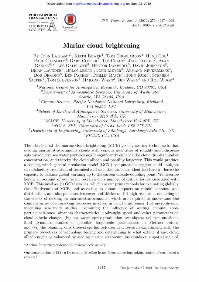
Meteorological conditions and cloud properties measured over the northeastPacific off the coast of California were used to initialize and constrain themodel simulations. In addition, the initial CCN number concentrations canbe varied to modify rain production in the modelled clouds, through whichthe aerosol can determine cloud cellular structures. Additional ship-emittedaerosols can further modify existing clouds. For example, figure 5 shows theimpact of ship emissions on clouds in both clean/precipitating and polluted/non-precipitating environments. An open-cell structure forms in the precipitatingcase. A ship track is clearly visible in the cloud albedo field (figure 5a) for theclean/precipitating case as would be expected even with Twomey’s argument.However, there are subtle changes in the cellular structure along the track fromthe plume head to tail, indicating that the interactions among ship-emitted CCN,clouds and precipitation vary with time. As revealed by Wang & Feingold [34],precipitation is suppressed most in the central section of the track, whereas newand sometimes stronger precipitation develops some distance behind the plumehead, resulting in restoration of the open-cell structure. This, together with theless reflective dark regions close to the lateral boundaries of the ship track,is caused by a mesoscale circulation owing to dynamical feedbacks associatedwith the initial suppression of precipitation along the ship track. Convergentbranches of the local circulation, located in the lower boundary layer over thetrack, pump moisture from the regions adjacent to the track and divergence inclouds helps dilute the ship-emitted CCN. Quantitatively, cloud albedo alongthe ship track was enhanced by 0.08 (averaged over 10 hours; [34]), while thedomain average albedo was only 0.015 higher than that of un-seeded clouds.
Phil. Trans. R. Soc. A (2012)
on June 23, 2018http://rsta.royalsocietypublishing.org/Downloaded from
Marine cloud brightening 4231
60
0 0.2 0.4 0.6 0.8
45
30
15
0
60
45
30
15
00 30 60
x (km)
y (k
m)
y (k
m)
90 120 150 180
(a)
(b)
Figure 5. Snapshots of the cloud albedo field when ships pass through the domain once fromx = 0 to 180 km, about 7 hours after the start of the simulations. The background aerosol numberconcentration varies linearly from a lower bound at x = 0 to an upper bound at x = 180 km; (a)clean case 60–150 mg−1 and (b) the polluted case 210–300 mg−1. Arrows indicate the direction ofmovement of the ships and the band of ship plumes emitted near the surface. Details on the modeland experimental set-up can be found in Wang & Feingold [33,34].
The dark edges (figure 5a) partly cancelled out albedo enhancement along theship track.
Although ship emissions are the same in the polluted/non-precipitating case,the ship track in figure 5b is nearly invisible because the relatively smallenhancement in cloud albedo (an average of 0.02; 4.3% relative to the domainaverage) is masked by the highly reflective cloud background. In addition, thereis no dynamical feedback associated with the interaction between the CCNperturbation and precipitation because the polluted cloud is non-precipitating.When averaged over the entire domain, the albedo enhancement in the pollutedcase becomes even smaller, 0.005.
Formed in a sufficiently polluted environment, closed cells as shown in figure 5bare over two times brighter than open cells in figure 5a. The most ideal outcomeof cloud seeding/brightening would be turning open cells into closed ones, assuggested by Rosenfeld et al. [38]. Can an influx of aerosols close open cells? Thereis no clear and firm answer yet. Numerical experiments conducted by Wang &Feingold [34] suggest that, once the open-cell structure is formed, simply addingmore aerosol particles, even in large quantities, does not necessarily transform itto a closed-cellular structure.
These high-resolution modelling studies suggest that seeding marinestratocumulus clouds, especially those that are precipitating, is morecomplicated than that predicated by the conventional aerosol indirect effects.The albedo response depends on meteorological conditions, background aerosol
Phil. Trans. R. Soc. A (2012)
on June 23, 2018http://rsta.royalsocietypublishing.org/Downloaded from
4232 J. Latham et al.
concentrations and seeding strategy, which together determine the spatialdistribution of injected aerosols and cloud properties, whether the cloudsprecipitate and therefore whether precipitation–suppression feedbacks canoperate. Using the same numerical model (WRF) and similar model settings,Wang et al. [16] describe more details of different meteorological andmicrophysical scenarios in this context, providing implications for experimentalstrategies to adopt in the field.
(c) Future of high-resolution cloud modelling in marine cloud brightening
The inability of global models to adequately represent MBL clouds andthe unresolved complexities of aerosol–cloud–precipitation interactions in suchclouds are major limitations in the assessment of the Earth system responseto future changes in climate, regardless of whether the change was causedinadvertently or was deliberately engineered. Improving our knowledge of suchprocesses should therefore be a major research goal, which relies much on high-resolution cloud modelling (e.g. LES and/or CRM). We suggest that any futureresearch programme on cloud brightening should include a high-resolution cloud-modelling component. More work is necessary to understand how ship trackssuch as those shown earlier form in response to idealized seeding strategiesunder different meteorological conditions and with different aerosol backgroundstates [16]. Beyond this, high-resolution modelling should be used to assessthe interaction of plumes from multiple seeding platforms such as those thatwould be necessary to deploy cloud brightening as a geoengineering scheme,regionally or globally. We currently have little idea on how clouds would respondto multiple aerosol plumes beyond what Wang et al. [16] have shown, and yetfigure 5a and Wang et al. [16] suggest that there are regions where the inducedmesoscale flows in the boundary layer act constructively and other regions wherethey destroy clouds, producing unintended consequences that reduce expectedalbedo response. In their 1 day simulations, Wang et al. [16] found that theinjection strategy is critical in determining the spatial distribution of the injectedaerosols and there is a case-dependent effective timing of injection during thediurnal cycle of marine stratocumulus. Longer time and more comprehensive high-resolution cloud modelling can be used to examine how rapidly induced aerosolperturbations from seeding are removed by coalescence scavenging and dilutionfrom entrainment of free-tropospheric air, providing guidance on the timing andduration of injection. These issues will be particularly pertinent when designingfield experiments to test critical aspects of cloud brightening.
4. Detailed modelling of the effects of sodium chloride spray oncloud–albedo change
The purpose of this section is to explore the range of dry salt masses andconcentrations that are most effective for altering the albedo of MBL clouds.
(a) Explanation of model and set-up of run
We have used a new cloud parcel model with size-resolved or bin microphysicsthat has been developed at Manchester, UK, and is called the aerosol–cloud and
Phil. Trans. R. Soc. A (2012)
on June 23, 2018http://rsta.royalsocietypublishing.org/Downloaded from

Marine cloud brightening 4233
precipitation interactions model (ACPIM) [39]. The work we have carried outhere builds on that previously reported in Bower et al. [3]. In their work, thecomposition of the background aerosol size distributions and that of the addedaerosol particles was prescribed to be sodium chloride. The added particles alsohad a single monomodal size. In this work, the size distributions of the backgroundaerosol distributions are the same as in Bower et al. [3] but are composed ofammonium sulphate to which sodium chloride particles are added in a mode offinite width to replicate more realistically the size distributions of particles thatcan be generated by the spray-production techniques described in §5b. The lowerlimit of added salt particle mass in Bower et al. [3] was 10−18 kg, sufficient to coverthe range of dry particle sizes under consideration by Salter et al. [4]. However,the range of the mass of added salt particles has now been extended to smallersizes, to encompass the size range that can be produced using the Taylor conetechnique (described later), which produces dry salt particles in the mass rangeof approximately from 3 × 10⁻²⁰ to 5 × 10⁻¹⁹ kg. Note that in the atmosphere itis well known that the dry salt particles would take on water and swell to largerphysical sizes as a result of the Raoult effect.
The parcel model version of the ACPIM used here activates aerosols ina sectional way. The ACPIM also uses a more thorough description of thethermodynamics of the aerosol [40] than was present in the NEATCHEM modelused in the Bower et al. study. Three sets of model runs were performed withACPIM; in each set of the runs, the control corresponded to running the modelwith a ‘background’ aerosol size distribution measured in three different airmasses (the ‘clean’, ‘medium’ and ‘dirty’ distributions used in Bower et al. [3]).Clean corresponds to a total number concentration of approximately 10 cm−3;medium approximately 260 cm−3; and dirty approximately 1000 cm−3.
Koehler theory was used to determine the equilibrium vapour pressure ofthe aerosols [40] in the background size distribution of particles (composed of(NH4)2SO4). The initial relative humidity, pressure and temperature in the modelwere set to 95 per cent, 950 hPa and 283.15 K, respectively, and the model wasrun until the parcel was lifted to a total height of 250 m. These conditions aretypical of stratocumulus clouds observed in the southeast Pacific Ocean thathave large spatial coverage (figure 1). Typically, this generated a cloud base(i.e. saturation level) approximately 75 m above the starting level and hence acloud approximately 175 m deep, allowing comparison with the results of Boweret al. [3]. Future work will look at the sensitivity of the addition of aerosols todeeper (i.e. more optically thick) clouds, although (as in the studies of Boweret al. [3]) the trends in albedo differences produced are expected to be similar.These simulations were repeated for different prescribed vertical wind speeds of0.2, 0.5 and 1.0 m s−1 to represent the typical range of updraught speeds found inmarine stratocumulus. Sensitivity tests were then performed investigating theeffect of adding a lognormal mode of aerosol to the background ammoniumsulphate aerosol distributions to simulate the spread in sizes expected fromthe droplet spray technique. The composition of the particles in the addedaerosol mode was NaCl, and their equilibrium vapour pressure was obtained fromKoehler’s theory.
The parameters varied in these tests were the total number of added aerosolparticles, nadd, and their dry salt mass ms. The parameter values used were nadd =0, 30, 300 and 1000 cm−3 and ms = 1 × 10⁻²⁰, 3 × 10⁻²⁰, 7 × 10⁻²⁰, 1 × 10⁻¹⁹,
Phil. Trans. R. Soc. A (2012)
on June 23, 2018http://rsta.royalsocietypublishing.org/Downloaded from

4234 J. Latham et al.
3 × 10⁻¹⁹, 7 × 10⁻¹⁹, 1 × 10⁻¹⁸, 1 × 10⁻¹⁷, 1 × 10⁻¹⁶, 3 × 10⁻¹⁶, 1 × 10⁻¹⁵ kg(or 1.06 × 10⁻², 1.53 × 10⁻², 2.03 × 10⁻², 2.29 × 10⁻², 3.30 × 10⁻², 4.37 × 10−2,4.92 × 10−2, 1.06 × 10⁻¹, 2.29 × 10⁻¹, 3.30 × 10⁻¹, 4.92 × 10⁻¹ mm dry aerosoldiameter, respectively). This range was chosen not necessarily because it spansthe range capable of being produced by the current spray generators (see §6), butbecause we wanted to determine where the main sensitivities lie. Addressing thiswill inform future spray generator development. The added lognormal mode wasspecified to have a median diameter equal to that of the added dry salt particles,that is
d̄ = 3
√6 mspr
. (4.1)
In all cases, the standard deviation of the mode was specified to be 0.25. Theparameter values listed totalled 41 runs per prescribed updraught value, a grandtotal of 369 runs (including runs with w = 1.0 m s−1, which lead to smallerparticles becoming activated; however, the results are essentially similar to thelower updraught cases, so they are not presented here). In principle, each of thespray techniques will probably yield its own unique size distribution of NaClparticles, but it is not clear yet what these are. Preliminary results show somesensitivity to the mode width; so it is intended to further investigate this in orderto inform spray technology engineers as to what tolerance is acceptable vis-à-visthis parameter.
In order to calculate the albedo for the simulation, we first calculated thevolume extinction coefficient, b(z), by integrating the product of the total cross-sectional area of the particles by their scattering efficiency (approximated as2 in this size regime, which is a reasonable approximation—see fig. 9.21 ofJacobson [41]),
b(z) = 2∑
i
Nipd2i
4, (4.2)
where Ni and di are the number concentration and diameter of the particles inbin i, and the sum is over every model size bin and each height level in the model.The solar optical depth, r , is then calculated by integrating the volume extinctionin the vertical,
t =∫
b(z)dz . (4.3)
The approximate broadband albedo, A, is then calculated using the formula (seeequation 24.38 of Seinfeld & Pandis [42])
A = t
t + 7.7. (4.4)
We report the total albedo change in this study that contains contributions fromthe direct effect and indirect effect. The direct effect is small when comparedwith the indirect effect in these calculations, and its magnitude will depend onthe amount of aerosol and the humidity.
Phil. Trans. R. Soc. A (2012)
on June 23, 2018http://rsta.royalsocietypublishing.org/Downloaded from

Marine cloud brightening 4235
100
100
200
300
40050
0
madd (kg)10−20 10−19 10−18 10−17 10−16 10−15
madd (kg)10−20 10−19 10−18 10−17 10−16 10−15
0
200
400
600
800
1000
0
200
400
600
800
1000
1010151520202525
30
30
35
35 40
0
200
400
600
800
1000
dA (
%)
dA (
%)
0
10
20
30
40
100
100
200
30040
050
060
0700800
0
200
400
600
800
1000
1010151520202525
30
30
35
35
40
0
10
20
30
40
(a) (b)
(c) (d)
activated drops, nact (w = 0.2 m s−1) activated drops, nact (w = 0.5 m s−1)
albedo change, dA (w = 0.2 m s−1) albedo change, dA (w = 0.5 m s−1)
n act (
cm−
3 )
n act (
cm−
3 )
n add
(cm
−3 )
n add
(cm
−3 )
Figure 6. Summary plots for the clean air mass. The number of activated drops without the additionof NaCl were 8.8 and 9.8 cm−3 for w = 0.2 and 0.5 m s−1, respectively. (a) A contour of the numberof activated cloud drops when a distribution of NaCl aerosols of different total number and medianmass are added to a rising parcel moving at 0.2 m s−1. The masses added are on the x-axis, whereasthe corresponding number added is on the y-axis. Plus signs denote the different runs used tocalculate the contour plot; (b) same as (a) but for an updraught of 0.5 m s−1; (c) the difference inthe albedo between the control run and the run with the indicated aerosol added (nadd, madd), inunits of per cent, of the clouds resulting from seeding; (d) same as (c) but for 0.5 m s−1. Pleaserefer to initial conditions in text for dry diameters corresponding to added dry particle masses.
(b) Results from model runs
Figure 6 shows results in the case where the background ammonium sulphatesize distribution is taken from that measured in a ‘clean air mass’ [3]. This caserepresents the most pristine conditions we might expect to find in the maritimeboundary layer. Concentrations in the medium case are slightly higher than foundover the southeast Pacific (e.g. during the recent VOCALS experiment). The dirtycase is very polluted. For the clean case, it can be seen (figure 6) that adding NaClparticles of dry mass less than approximately 1 × 10⁻¹⁹ kg results in no changeto the cloud drop number because these particles have too high curvature andtoo low solute mass to be active CCN. Adding particles of dry mass greater thanapproximately 1 × 10⁻¹⁶ kg results in aerosols not activating to form cloud drops(figure 6a,b). However, the added sodium chloride aerosols, while not ‘classically’activating (to form cloud drops), still take on appreciable liquid water, swelling tosizes approaching approximately 10 mm. The result of this is a thick haze havinghigh extinction of solar radiation and hence a high albedo, as can be seen fromfigure 6c,d. The pre-existing ammonium sulphate aerosols have their activation
Phil. Trans. R. Soc. A (2012)
on June 23, 2018http://rsta.royalsocietypublishing.org/Downloaded from

4236 J. Latham et al.
dA(%
)
dA(%
)dA
(%)
dA(%
)
−202
2
4466
8
8
10
10
12
12
14
14
16
16 1820
albedo change, dA, (medium, w = 0.2 m s−1)
0
200
400
600
800
1000
0
5
10
15
20
0
22
44668
8 10
10 12
12 14
1416
1618
20
0
5
10
15
20
−4−2−2
0
0
2
2 4
4 6
68
810
10
12
14
albedo change, dA, (dirty, w = 0.2 m s−1)
10−20 10−19 10−18 10−17 10−16 10−150
200
400
600
800
1000
0
5
10
15
20
−2−2
−2
0
0
2
2
4
4
6
6 810
0
5
10
15
20
(a) (b)
(d)(c)
n add
(cm
−3 )
n add
(cm
−3 )
albedo change, dA, (medium, w = 0.5 m s−1)
albedo change, dA, (dirty, w = 0.5 m s−1)
madd (kg)10−20 10−19 10−18 10−17 10−16 10−15
madd (kg)
Figure 7. Summary plots of the albedo change for the medium and dirty air-mass cases. For themedium case, the number of activated drops without the addition of NaCl were 142 and 179 cm−3
for w = 0.2 and 0.5 m s−1, respectively, whereas for the dirty case these were 358 and 639 cm−3 forw = 0.2 and 0.5 m s−1, respectively. (a) The difference in the albedo between the control and therun with the indicated aerosol (nadd, madd) for the medium case with 0.2 m s−1 updraught; (b) thesame but for 0.5 m s−1; (c, d) the corresponding contours of albedo change for the dirty case.
suppressed. Between 1 × 10⁻¹⁹ and 1 × 10⁻¹⁶ kg dry mass, we are able to alterthe modelled cloud drop concentration very effectively by changing the numberconcentration of added aerosols. Although the addition of NaCl particles of massgreater than 1 × 10⁻¹⁶ kg results in no aerosols being activated as CCN, theswelling of these aerosols still has the desired effect of increasing ‘cloud’ albedo,regardless of whether they are activated. However, adding aerosols of this size orgreater (which are effectively giant CCN) may result in undesirable effects suchas the more efficient production of rain; an effect that will be investigated infuture work). The maximum change in albedo for the clean air mass is around0.4, rising from an albedo of 20 per cent for the control to 60 per cent for thecase in which high concentrations of large NaCl particles have been added.
The pattern of aerosols not strictly being activated but still contributing toalbedo difference was observed in both the medium and dirty cases, so the plotsof cloud drop number are not shown here.
Figure 7a,b shows the model results for the medium loading ammoniumsulphate background air-mass case [3]. Qualitatively, the results are similar tothe cleaner air-mass results except for two key differences: (i) the magnitudeof albedo difference is about a factor of 3 smaller than in the clean case and(ii) for the lower updraught case (w = 0.2 m s−1) adding relatively few large NaCl
Phil. Trans. R. Soc. A (2012)
on June 23, 2018http://rsta.royalsocietypublishing.org/Downloaded from

Marine cloud brightening 4237
particles may actually reduce the albedo of the clouds by a small amount. Thereason for this is that a few large NaCl particles are able to reduce the peaksupersaturation in the rising parcel enough to reduce the number of cloud dropsin the background spectrum that would otherwise activate to form cloud drops,but not enough to suppress activation entirely. This reduction in turn reducesthe extinction of the clouds as there are fewer, larger particles than in the controlcase. Suppressing activation entirely (i.e. when adding many large NaCl particles)results in many large swollen aerosol particles and hence larger extinction, as canbe seen from figure 7a,b. In the absence of seeding, the concentrations of clouddroplets generated in the background in the clean, medium and dirty cases were8.8, 142, 358 cm−3, respectively, for an updraught of 0.2 m s−1, and 9.8, 180 and639 cm−3, respectively, for an updraught of 0.5 m s−1.
Figure 7c,d shows the model results for the case in which there is a highconcentration of background ammonium sulphate aerosol present, correspondingto a ‘dirty air mass’. Qualitatively, the results are much the same as for boththe clean and the medium air mass cases. One difference is that the albedo ofthe clouds is now less susceptible to the inclusion of additional sea salt aerosol.There was little increase in cloud droplet number even when adding particlesapproaching 1 × 10⁻¹⁸ kg in mass, especially for the low-updraught case (notshown here).
In the medium and clean cases, a larger increase in cloud droplet numberwas found for the addition of NaCl aerosol of this or even smaller mass. Thereason for this decreased sensitivity is that, in the dirty case, there are alreadycopious (NH4)2SO4 particles present in the background aerosol to deplete thesupersaturation at cloud base such that the NaCl particles of approximately 1 ×10⁻¹⁸ kg cannot be activated. Similarly, the point at which drops cease to beactivated has also changed. In the previous cases, drops ceased to activate whenNaCl particles of mass approximately 1 × 10⁻¹⁶ kg (or larger) were added. In thiscase, activation of additional drops ceases at a lower threshold sea salt particlemass (typically 7 × 10⁻¹⁷ kg or less). This is because the higher concentration ofbackground aerosol contributes significantly to the reduction in supersaturation inthe rising parcel of air, suppressing further activation. Another notable differenceis that the maximum change in albedo that is achieved is considerably less thanfor the clean case, and slightly less than in the medium case too. More noticeablein this case is a region where a reduction in albedo occurs when adding relativelyfew large-mass NaCl particles.
(c) Conclusions
The modelling suggests the following:
— The enhancement to the albedo is greatest for clean background conditions.This is consistent with previous work by Bower et al. [3].
— In the clean conditions, the albedo of the control case cloud wasapproximately 20 per cent, whereas for the case where many large NaClparticles were added it was approximately 60 per cent. This (factor of 3)difference should be easily observable in a field campaign. In the mediumand dirty cases, these increases in albedo were a factor of 1.6 and 1.3,respectively. This corresponds to albedos in the control runs for the
Phil. Trans. R. Soc. A (2012)
on June 23, 2018http://rsta.royalsocietypublishing.org/Downloaded from

4238 J. Latham et al.
medium and dirty cases of 35 per cent and 45 per cent with the maximumabsolute increases in albedo of 20 per cent and 12 per cent, respectively.The magnitude of these changes will vary slightly with cloud depth(although the trends will be similar), and this will be investigated in futurework.
— The values of the albedo in the control runs are typical of observedstratocumulus clouds and are in the same range as those in the cloudmodelling section (figure 5).
— For both the medium and dirty cases, a reduction in cloud albedo wasfound when adding relatively low concentrations of particles that haveNaCl masses of approximately 1 × 10⁻¹⁶ and greater. This underscoresthe findings by Bower et al. [3] that, for efficient albedo enhancement,the added particles should have masses higher than almost all naturalparticles and be added in significantly greater numbers; however, currenttechnology is unable at present to generate such large particles insignificant concentrations (see §6). Nevertheless, this study has shown thatadding smaller particles of 3 × 10⁻¹⁹ kg (0.033 mm) results in smaller, butstill significant, albedo enhancement. Furthermore, adding particles of saltmass less than 1 × 10⁻¹⁹ kg in the clean and medium cases and less than1 × 10−18 in the dirty case produced little change to the drop number.
— While the most efficient albedo enhancement is achieved by adding largeNaCl particles, it should be noted that such large particles may alsoinitiate rain that is detrimental to cloud brightening as it tends to reducecloud lifetime [13]. This effect needs further investigation both withhigh-resolution models (see §3) and further parcel modelling.
When performing this study, we chose conditions to be relevant to those thatseed aerosols would experience as they rise through a stratocumulus cloud layerin the southeast Pacific Ocean and hence we are limited as to the generality ofour conclusions. We expect that, in general, the results would not be too differentin all marine stratocumulus clouds. However, it is noted that the scheme will notbe as effective in marine stratocumulus clouds that are close to significant sourcesof anthropogenic aerosol.
5. Engineering steps to implement marine cloud brightening
(a) Introduction
Previous sections have considered the science of cloud brightening by increasingthe CCN of marine stratus clouds (by way of a very fine, evaporating spray of seawater microdroplets) and the foreseen impact on global climate. In this section,attention is turned to what are seen as the two major technological challengesthat have a vital bearing on the effectiveness: the time scale for developmentand the overall costs of the scheme. These are, first, how one might generate themist of microdroplets of the desired size and spray-rate needed and, second, whatstrategy should be adopted for delivering the spray; for example, whether frommobile or stationary sources and, if from a mobile source (i.e. a ship), the typeof vessel and the optimum means of propulsion.
Phil. Trans. R. Soc. A (2012)
on June 23, 2018http://rsta.royalsocietypublishing.org/Downloaded from

Marine cloud brightening 4239
In fact, both these aspects were considered, if not entirely resolved, by Salteret al. [4] and this section mainly concentrates on new developments. That paperhad already concluded that sea-level dispersal of an evaporating spray haddecisive advantages over the more direct approach of cloud seeding from aircraftand that, among the several alternative strategies, dedicated sea-going vesselspropelled by Flettner rotors (which facilitated an unmanned operation) were thepreferred technical choice as well as being, by a considerable margin, the cheapestand ‘greenest’ route. The performance of Flettner rotors had not, however, beenexamined for more than 80 years and thus in §5c our first results based on CFDof the dynamic performance of a single rotor are presented. This is preceded, in§5b, by an even more pressing issue—the approach to be used for producing thesalt-water spray.
(b) Electrohydrodynamic spray fabrication
We have explored experimentally a number of ways to produce sea waterdroplets that would be suitable for use in cloud brightening. The criticalrequirement is that their salt mass ms be high enough that they can convertinto cloud droplets at the supersaturation, S , occurring in marine stratocumulusclouds. S depends on updraught speed, and the properties of the air mass. Cloudmodelling (described later) provides values of critical mass for a variety of relevantscenarios. They show that significant droplet formation and associated cloudalbedo increase can occur for ms values down to about 5 × 10⁻²⁰ kg. Hence,the initially sprayed droplets, drying to a quarter of their initial size, shouldminimally be of the order of 150–200 nm diameter. For energy efficiency, it isadvantageous to make the droplets close to this lower acceptable limit, for it isthe number of suitable nuclei formed, not the amount of water sprayed, that isimportant. The smaller the size of the droplets capable of inducing activation, thesmaller the required amount of spray with its associated energy and evaporativeair cooling.
We investigated the performance of standard commercial nozzles that are usedin fogging systems, toroidal vortex-based nozzles, colliding water jets, ultra-high-pressure nozzles (345 MPa) and Rayleigh-mode jet break-up from micromachinedand radiation-track apertures. These experiments will be detailed in anotherpublication, but, so far, none has produced encouraging results.
The best results to date were obtained using Taylor cone-jets [43], drawnfrom porous tips. Upon application of a voltage to a capillary containing afluid, the most interesting of the spraying modes is the cone-jet, i.e. a coneterminating in an emerging jet. The 49.3◦ half-angle cone first described by Tayloris well understood, but the jet description is much more complex, particularly forhigh-conductivity liquids such as sea water. Analysis by De la Mora [44] andGañán-Calvo & Montanero [45] show that a critical radius (ri) exists, defined bythe flow and the dielectric relaxation constant of the fluid. A highly charged jet ofapproximate radius 0.2 ri emerges and breaks up monotonically, similar to thatof an uncharged Rayleigh jet. Each drop is often accompanied by a satellite drophaving a mass a few per cent of that of the parent drop.
Figure 8 shows scanning electron microscope (SEM) images, at differentmagnifications, of salt particles produced by a Taylor cone emanating from aporous tip, collected on a silicon wafer at a 5.4 kV potential, a current of 0.2 mA
Phil. Trans. R. Soc. A (2012)
on June 23, 2018http://rsta.royalsocietypublishing.org/Downloaded from

4240 J. Latham et al.
Figure 8. SEM images of salt particles from salt-water cone-jets at different magnifications.
with a flow of 5.6 nl s−1, using 540 ppm of surfactant. The surfactant lowers theinstability threshold below air breakdown, eliminating the corona discharge thatdestroys the uniformity of the particle distribution. The average size of thesecrystals is of the order of 75–85 nm, having a mass of approximately 10−18 kg,suitable for the intended purpose. The droplets evaporate before they reach thesilicon wafer 2 cm away. This near instantaneous evaporation of the droplets is dueto their emergence from the jet with velocities approaching the speed of sound,and the heating that takes place in the cone itself [46]. These crystals readilyconvert at a supersaturation of 0.5 per cent, achieved by cooling the wafer witha thermoelectric chuck in an enclosed environment.
Although each cone-jet produces a very large number of droplets (of the order of108–109 s−1), scale-up requires 108 jets to reach roughly 1017 nuclei s−1 per sprayer.Small arrays of porous tips work well, but the overall size would be prohibitive.Various efforts have been made to mass produce cone-jet capillaries and associatedextraction plates. Perhaps the most relevant for our purposes is the work of Denget al. [47], who described the micromachining of silicon capillaries and extractionplates, alignment methods and the production of arrays with up to 331 nozzles,producing remarkably uniform spray, with only a few per cent of size deviation.The density of the capillaries exceeds 100 mm−2, suggesting approximately 1 m2
in total for the nozzle array that is technically feasible by tiling.As a low-cost alternative, we have pursued the use of holes in low-dielectric
polymeric materials (PEEK, polyimide, PMP) in place of capillaries. Thisapproach was first outlined by earlier studies [48,49]. This technique lowers powerconsumption, and the fabrication of holes is significantly easier than that ofcapillaries. These holes must have a large aspect ratio in order to avoid interactionbetween adjacent holes. The problem can be overcome by using a dielectricthin film (50–75 mm) attached to a porous block that provides flow impedance,isolation and filtration at the same time. Such arrays may then be made by fastand inexpensive laser drilling systems. To fabricate prototypes we were able tomake use of a Samurai UV marking system (courtesy of DPSS Lasers Inc., SantaClara, CA), capable of drilling 50 000 holes s−1. Hence, the drilling of 100 millionholes is a manageable task, requiring a hole every 100 mm over a total area of 1 m2.
The other requirement [48] is that the water needs to be confined at the rimof each individual hole, or jets will coalesce. To this end, it has been found thatthe dielectric material needs to be made superhydrophobic, i.e. the fluid contact
Phil. Trans. R. Soc. A (2012)
on June 23, 2018http://rsta.royalsocietypublishing.org/Downloaded from

Marine cloud brightening 4241
angle must be in excess of 150◦ [11]. Polyimide films were made superhydrophobicby plasma etching with oxygen, yielding a rough surface, followed by plasmadeposition of a 20 nm fluorocarbon film. The combination gives rise to thedesired surface properties, with water contact angles approaching 160◦. However,the surfactant needed to obtain reliable cone-jet spraying of sea water lowersthe contact angle to values that are unacceptable. Using films made at theStanford Nanofabrication Facility or supplied by commercial sources (Repellix;Integrated Surface Technologies, Inc., Menlo Park, CA), we were unable to finda combination of surfactant and robust surface preparation that satisfies all therequirements.
The surfactant requirement can be eliminated by a number of methods:increased ambient pressure or smaller apertures. If the ambient pressure is raisedslightly (20%), the air breakdown field increases. With slight over-pressurization,corona discharge disappears and there is no need for surfactants. Raising thepressure causes airflow through the extraction apertures and, while the flowthrough each hole is small, an array of 100 million holes demands a substantialamount of power. The flow of air is of course beneficial in helping the passageof the droplets through the extractor holes. Likewise, when the capillary holesare made smaller than 10 mm, the air breakdown field (increasing with decreasingjet radius) is at all times higher than the field over the cone itself; so no airbreakdown occurs here either.
In summary, the fabrication of large arrays of Taylor cones, either by siliconmicromachining or by laser drilling in dielectric sheets, seems quite feasiblealthough no such large arrays have yet been constructed. It is estimated that foran array of 100 million holes, roughly 1 m2 in size, the electrical power requirementwould be less than 100 kW. If airflow is used, then there would be an additionalrequirement of 270 kW for pneumatic power. Because more than 90 per cent ofthe electrical power ends up as droplet kinetic energy, it can probably be partiallyrecovered by reverse induction using a Kelvin generator arrangement.
As a simpler alternative, we are exploring the spraying of sea water at or nearits critical point. In this regime, water has little or no surface tension and a gas-likeviscosity and hence should produce fine dispersions. This has been demonstratedin the pharmaceutical industry with the spraying of supercritical carbon dioxidecontaining dissolved therapeutic compounds. While the distributions resultingfrom this technique are bound to be wider than those from cone-jets, the resultantparticle distribution can on occasion be quite uniform [50]. Results of thisinvestigation will be reported later.
We used the model described in §4 to examine in more detail the conditionsunder which the electrohydrodynamic spraying technique could produce albedochange values of significance (i.e. not less than about 0.06, or 6%). We present intable 1 the change in albedo (for each air mass) that could be achieved by adding1000 cm−3 of NaCl particles of mass within the range currently achievable bythis technique (i.e. up to about 10−19 kg). We present only the 1000 cm−3 resultsbecause our model results showed that this led to the maximum change in albedo.It can be seen that the technique can result in large albedo change in clean airmasses. For the medium-polluted air mass, only particles of salt mass larger thanor equal to approximately 3 × 10⁻¹⁹ kg result in an albedo change that may besignificant for offsetting warming by carbon dioxide, whereas for the dirty airmass all salt masses result in negligible albedo change.
Phil. Trans. R. Soc. A (2012)
on June 23, 2018http://rsta.royalsocietypublishing.org/Downloaded from

4242 J. Latham et al.
Table 1. DA values (in %) achieved in the 0.2 m s−1 updraught case for runs where 1000 particlesof NaCl per cm3 were added in the range 1 × 10⁻²⁰ to 3 × 10⁻¹⁹ kg.
air mass mass (kg) 1 × 10⁻²⁰ 3 × 10⁻²⁰ 7 × 10⁻²⁰ 1 × 10⁻¹⁹ 3 × 10⁻¹⁹
clean 3.9 16 20 25 28medium 9.1 × 10⁻³ 3.8 × 10⁻² 5 × 10⁻¹ 1.4 6.5dirty 1 × 10⁻² 2.3 × 10⁻² 4.7 × 10⁻² 6.5 × 10⁻² 1.8 × 10⁻¹
This highlights that, in very clean clouds, the electrohydrodynamic spraytechnique is feasible. However, in the medium and in the dirty air masses,in particular, we would probably need to produce larger particles of (around1 × 10−18 kg), as suggested by figure 6.
(c) Computational fluid dynamics studies for optimizing the Flettnerpropulsive system
(i) Scene setting
The most direct and probably the most obvious route for supplying theadditional CCN would seem to be by directly seeding the microparticlesfrom aircraft flying below the bases of the marine clouds to be brightened.Our earlier work on MCB [4,5] had firmly concluded, however, that sea-levelinjection of microdroplets of sea water would be as effective while offering majorenvironmental and cost-saving benefits. Among the sea-level options for seedingthe marine clouds, fixed spraying locations from anchored platforms would haveto be too numerous to provide a reasonable coverage of the most suitable regionsand their servicing at sea would be both hazardous and expensive. While thespraying equipment could be installed on regular cargo vessels as they plied theoceans, Salter et al. [4] concluded that it was better to have a vessel—or, rather,fleet of vessels—dedicated to the task of cloud seeding. Given the unusual role thatthese craft had to play, however, it was imperative that the ship’s design be opento possibly radical innovations. The most important of these was the proposalthat the vessel should be propelled not by conventional diesel engine-poweredpropellers nor by sails, but by Flettner rotors.
A Flettner rotor (named after its inventor, Anton Flettner) is a verticallymounted cylinder that may be rotated about its axis by an external power supply.When air flows past it, the cylinder rotation creates a force (the Magnus force)at right angles to the air flow that propels the vessel on which the cylinder ismounted. The rotor thus plays the same role as the sails on a yacht but the thrustlevels attainable are far greater than for a sail of the same area; moreover, thecontrol of such vessels is very much simpler (without the complex rigging of a sailand with far superior manoeuvrability). This latter feature makes vessels poweredby Flettner rotors ideal for unmanned, radio-controlled operation, a measure thatclearly brings enormous savings in costs for it dispenses with the need for a crewand the associated multi-faceted support infrastructure. Moreover, it has beenestimated [4] that the cost of providing the power to spin the rotor is an orderof magnitude less than that required for a screw-driven vessel of comparable size
Phil. Trans. R. Soc. A (2012)
on June 23, 2018http://rsta.royalsocietypublishing.org/Downloaded from

Marine cloud brightening 4243
Figure 9. Artist’s impression of a Flettner rotor ship. Reproduced from Gadian et al. [51]. (Onlineversion in colour.)
sailing at the same speed. The fact that that speed would usually be less than halfthat of a diesel-powered craft in normal operation is immaterial for the purposeof cloud seeding.
An artist’s impression of such a vessel is shown in figure 9. While the originalFlettner vessel that crossed the Atlantic in 1926 was propelled by two purelycylindrical rotors, in the conceptual design of the cloud-seeding craft shown inthe figure, the rotors have a number of discs mounted along their length. In fact,Thom [52] carried out a number of wind-tunnel experiments that suggested thatthe inclusion of such discs markedly improved rotor performance at high spinrates. Inevitably, however, the scope of that experimental exploration was limitedand was certainly not conceived as contributing to the particular requirementsof the cloud-seeding craft. Moreover, nearly 80 years on, as in so many areas,computer simulation (while not replacing the need for experiments) has made itfeasible to explore a wide range of flow conditions and rotor geometries relativelyrapidly and to provide far greater detail than any experiment. Here, therefore,our first results of applying CFD to the Flettner rotor problem are presented.
Phil. Trans. R. Soc. A (2012)
on June 23, 2018http://rsta.royalsocietypublishing.org/Downloaded from

4244 J. Latham et al.
The first major computational study into the behaviour of flow past a rotating(bare) cylinder was undertaken by Mittal & Kumar [53] (hereafter M&K). Whilethat study was limited to laminar flows at a Reynolds number, U∞D/v (5.1),1 of200 (i.e. two or three orders of magnitude below those that would be encounteredin an actual cloud-seeding vessel), their results revealed a potentially worryingfeature with a major bearing on the present research. Over a limited rangeof rotation rates (relative to the wind speed), the flow around the cylinderexperienced large-scale temporal periodicities that produced highly undesirablevariations in drag and lateral forces on the cylinder. If these were present underoperational conditions in the cloud-seeding vessel they would, inter alia, have aseriously adverse effect on the lifetime of the rotor and its support mechanisms.Thus, in the exploratory studies presented later of turbulent flow past the rotorat Reynolds numbers typical of operating conditions, such flow instabilities havebeen a major feature to watch out for.
(ii) Numerical and physical model
Computations have been performed using an in-house CFD solver,STREAM [54], to examine the flow around rotating cylinders with and withoutThom discs. For these tests, the discs have been taken as flat annular platesof diameter twice that of the cylinder, axially spaced, one cylinder diameterapart. (This corresponded with the spacing shown in figure 9, although in Thom’soriginal tests the disc diameter was three times that of the rotor and the axialspacing just half the rotor diameter.) The results presented here have beenobtained using a multi-block, non-orthogonal grid (figure 10) of around 0.75 Mcells, covering a domain extending far enough from the cylinder for boundaryeffects to be negligible, and extending vertically from one disc to the next, asshown in figure 10. A uniform ‘wind’ velocity was specified around the inlet partof the outer boundary and zero-gradient conditions on the outlet. Symmetryconditions were applied along the two boundaries normal to the cylinder, andno-slip conditions, via ‘wall functions’, were applied at the disc and cylindersurfaces. For comparison, simulations were also performed for a bare cylinder(i.e. without discs).
For most of the test cases, the effects of turbulence were represented by aconventional k–3 linear eddy viscosity model with standard log-law-based ‘wallfunctions’ to provide the wall boundary condition. Some runs have, however, beenmade using more advanced stress-transport turbulence models and wall-functiontreatments (summarized, for example, in Craft et al. [55]). Although there aresome modest quantitative differences in results between the different modellingapproaches, cross checks show very similar trends, and because of the two- orthreefold time penalty with the more elaborate model, most results were obtainedwith the simpler eddy viscosity scheme.
(iii) Initial computational results
To validate the procedure, purely laminar flow around a bare rotor for aReynolds number of 200 was examined, corresponding to the case studied byM&K. In agreement with their results, the present computations confirmed that1U∞ is the wind velocity past the rotor of diameter D and n is the kinematic viscosity of the air.
Phil. Trans. R. Soc. A (2012)
on June 23, 2018http://rsta.royalsocietypublishing.org/Downloaded from

Marine cloud brightening 4245
Figure 10. Details of the multi-block, non-orthogonal mesh. (Online version in colour.)
the Karman vortex street, present behind non-rotating cylinders, disappearedfor dimensionless rotation rates, U ≡ uD/(2U∞), greater than 2 (where u is theangular velocity of the cylinder). Moreover, for a narrow band of rotation ratesaround U = 4.4, longer period, large-amplitude oscillations developed, althoughby U = 5 these also disappeared, again broadly in agreement with the M&Kresults. As noted already, a major question in the present context is whether theseinstabilities also arise in turbulent flow at the much higher Reynolds numberscommonly encountered for a Flettner rotor.
The presently predicted results for turbulent flow at Re = 8 × 10⁵ aresummarized in figure 11, which shows the dependency of the rotor’s lift coefficient,CL, on the non-dimensional rotation rate. For zero rotation, the bare cylinderresults display the expected oscillatory pattern associated with the Karmanvortex street. As the rotation is increased, these oscillations disappear, and themagnitude of CL increases steadily. By a rotation rate of U = 5, a lift coefficientof around 12 is predicted. Although rather less than half the corresponding valuefound for laminar flow, this is still sufficiently high to underline the value ofthe Flettner rotor as a propulsive device. A further point to note from thebare cylinder results is that the large-amplitude oscillations seen in the laminarflow calculations around U = 4.4 were not detected in the turbulent case for therotation rates examined. However, as can be seen from figure 11, at rotation ratesabove U = 3, the solution did not exhibit an entirely steady behaviour, indicatingthat there are nevertheless unsteady three-dimensional structures present in theflow, although not in an organized, regularly repeating form.
Turning now to the effects of the Thom discs, the time histories of the liftcoefficient, also included in figure 11, indicate that the mean values of CL are notvery different from those of the bare cylinder. A feature worth noting, however,is that, by including the discs, a much steadier flow field is achieved. For the case
Phil. Trans. R. Soc. A (2012)
on June 23, 2018http://rsta.royalsocietypublishing.org/Downloaded from

4246 J. Latham et al.
0 100 200 300time
0
–5
–10
–15
CL
W = 0
W = 3
W = 5
solid lines: bare cylinder
broken lines: with Thom discs
Figure 11. Predicted temporal evolution of experimental lift coefficient for turbulent flow atRe = 8 × 10⁵ for a range of rotation. (Online version in colour.)
of no rotation, the Karman vortex street is suppressed, and a constant value ofCL (zero) is thus returned. At rotation rates of U = 3 and 5, although there aresome small undulations in the CL time history, these are very minor (and fairlyperiodic) compared with the behaviour of the bare cylinder.
Figure 12 compares the predicted mean lift coefficient, as a function of rotationrate, with and without discs and the very early (but still among the mostcomprehensive) measurements of Reid [56] for a bare cylinder. The experimentaldata for the bare cylinder show a fairly rapid rise in CL as U is increased from 0to around 3, followed by a more moderate rate of increase thereafter. The presentresults broadly reproduce this pattern. The numerical results show values slightlyhigher than the measurements. As noted earlier, the calculations show only minordifferences in average CL values between the cases with and without Thom discs.
Finally, the question of whether large-amplitude periodicities may arise cannotyet be answered definitively. The computations of M&K and our own showthat, in the laminar-flow regime, these instabilities appeared only over a verynarrow range of spin rates. Preliminary turbulent flow studies have suggestedthat such oscillations may also occur [57] again over a narrow range of conditions.Further extensive explorations are required, however, before firm conclusions canbe reached.
(iv) Examples of future work
Readers will recognize that the results shown earlier, while containinginteresting and encouraging pointers, represent just a start on a range of CFDcomparisons that will need to be made. As a first step, the computations need toconsider a complete rotor rather than just the section between one disc and thenext. This will enable the exploration of end effects and the possible variation withheight of the wind velocity to be examined as well as potential interference effects
Phil. Trans. R. Soc. A (2012)
on June 23, 2018http://rsta.royalsocietypublishing.org/Downloaded from
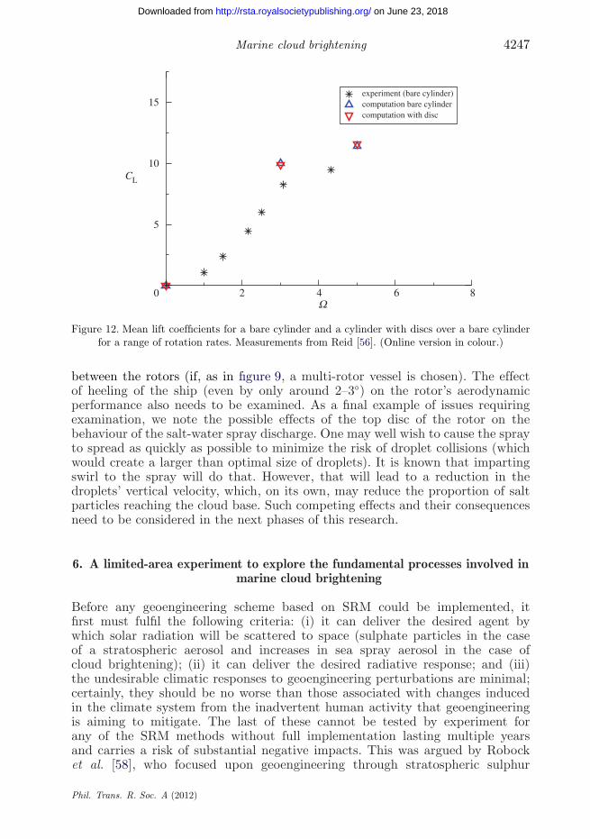
Marine cloud brightening 4247
CL
42 6 8W
0
5
10
15experiment (bare cylinder)computation bare cylindercomputation with disc
Figure 12. Mean lift coefficients for a bare cylinder and a cylinder with discs over a bare cylinderfor a range of rotation rates. Measurements from Reid [56]. (Online version in colour.)
between the rotors (if, as in figure 9, a multi-rotor vessel is chosen). The effectof heeling of the ship (even by only around 2–3◦) on the rotor’s aerodynamicperformance also needs to be examined. As a final example of issues requiringexamination, we note the possible effects of the top disc of the rotor on thebehaviour of the salt-water spray discharge. One may well wish to cause the sprayto spread as quickly as possible to minimize the risk of droplet collisions (whichwould create a larger than optimal size of droplets). It is known that impartingswirl to the spray will do that. However, that will lead to a reduction in thedroplets’ vertical velocity, which, on its own, may reduce the proportion of saltparticles reaching the cloud base. Such competing effects and their consequencesneed to be considered in the next phases of this research.
6. A limited-area experiment to explore the fundamental processes involved inmarine cloud brightening
Before any geoengineering scheme based on SRM could be implemented, itfirst must fulfil the following criteria: (i) it can deliver the desired agent bywhich solar radiation will be scattered to space (sulphate particles in the caseof a stratospheric aerosol and increases in sea spray aerosol in the case ofcloud brightening); (ii) it can deliver the desired radiative response; and (iii)the undesirable climatic responses to geoengineering perturbations are minimal;certainly, they should be no worse than those associated with changes inducedin the climate system from the inadvertent human activity that geoengineeringis aiming to mitigate. The last of these cannot be tested by experiment forany of the SRM methods without full implementation lasting multiple yearsand carries a risk of substantial negative impacts. This was argued by Robocket al. [58], who focused upon geoengineering through stratospheric sulphur
Phil. Trans. R. Soc. A (2012)
on June 23, 2018http://rsta.royalsocietypublishing.org/Downloaded from

4248 J. Latham et al.
injection, currently considered to be one of the most feasible schemes [59]. Robocket al. [58] further argued that it is impossible to fully field test geoengineeringschemes without significant modification to the climate system owing to non-localclimate responses.
While we agree that large-scale field testing of any geoengineering scheme isindeed inseparable from deployment, small-scale field testing will be necessaryto make significant progress in understanding the feasibility of geoengineeringschemes [60]. An attractive aspect of MCB in terms of field testing is that,because aerosol particles in the MBL are extremely short-lived (typically a fewdays) compared with their stratospheric counterparts (1–2 years), perturbationsto the radiative budget from MCB are inherently localized. This is not the casewith stratospheric sulphur injection. This essentially means that it is possible toconduct a useful test of MCB (with minimal climate impacts) over a limited areathat includes testing of TOA radiative responses in addition to the testing ofinjection methodologies and dispersion, etc. This is in contrast to stratosphericsulphur geoengineering, in which case, as Robock et al. [58] correctly argued, itwould be extremely difficult to measure either an effect on the Earth’s radiationbudget or maintenance of the aerosol in the stratosphere using only a smallnumber of injections that might constitute a field test.
The stratospheric sulphur injection scheme has so far been considered one ofthe most viable schemes, not least because previous volcanic eruptions such asPinatubo in 1991 have provided significant data against which model predictionsof the radiative effects of sulphate particles in the stratosphere can be testedand validated [61,62]. Unlike stratospheric aerosols, many of the basic processeslinking tropospheric aerosols, clouds, precipitation and radiation underpinningthe cloud-brightening scheme are rather poorly understood [15]. Given that theinfluence of human activity on such processes has been proposed to make asubstantial contribution to the radiative balance [63,64], it is imperative thatbasic knowledge of aerosol–cloud interactions is improved substantially, regardlessof the viability of cloud brightening as a geoengineering scheme.
Inadvertent human-induced changes to regional aerosol particle burdens havebeen used to investigate these processes in regions of stratocumulus in thepast [65,66], though large natural variability and co-dependency of processes hasto date limited progress towards full understanding. Also, emissions from thestacks of ships have been used to study aerosol–cloud interactions [67], but singleplumes of this type can provide only limited information as plumes are narrowand entrainment and mixing are often dominant. A limited-area field experimentthat provides a substantial and detectable perturbation above the background onspatial scales that are detectable from space could therefore offer a unique way toprobe aerosol–cloud–precipitation interactions, and their influence on radiation.It would also enable new knowledge on aerosol influences on climate to be gained.
An analogy can be drawn between improving knowledge of aerosol–cloudinteractions through a limited-area perturbation experiment and previousexperiments conducted to investigate the control of micronutrients (notablyiron) on the drawdown of carbon by marine biological systems. A number ofexperiments have been conducted, which have deliberately added iron to theocean to improve knowledge of ocean biological carbon cycling. These havesubstantially improved knowledge of nutrient limitation on oceanic primaryproduction, its subsequent control on plankton communities and how this impacts
Phil. Trans. R. Soc. A (2012)
on June 23, 2018http://rsta.royalsocietypublishing.org/Downloaded from

Marine cloud brightening 4249
on cycling of carbon and nitrogen in the world’s oceans [68]. Further fertilizationexperiments to develop knowledge of the fundamental processes are seen as crucialto furthering the understanding of the Earth system and are critical before anyconsideration is given to large-scale deliberate attempts at carbon sequestrationby such means [69]. A major concern is that larger scale experiments may havesignificant impacts on ocean ecosystems. A key point is that a limited-area fieldexperiment to study aerosol–cloud interactions using artificially generated aerosolfrom sea spray can be carried out without any climatically damaging effects as thelifetime of atmospheric aerosol in the MBL is of the order of a few days at most.Such experiments therefore offer a valuable contribution to climate science andshould not be viewed as solely a means of validating the cloud-brightening scheme.
Here, we present an initial framework for the testing and implementation ofsuch experiments. We propose a set of field tests to critically assess the efficacy ofMCB over a limited area. The tests are de minimus with respect to their climateeffects, as we shall discuss later. The tests involve three phases, with increasinglogistical complexity, each of which is designed to test one or more importantcomponents of the cloud-brightening scheme. Each involves the introductionand monitoring of controlled aerosol perturbations from one or more ship-basedseeding platforms up to a limited area of approximately 100 × 100 km2. A suite ofobservational platforms of increasing number and complexity, including aircraft,ships and satellites, will be required to observe the aerosol plume and in the latterexperiments the cloud and albedo responses to the aerosol perturbations. Theseinclude the necessary cloud physical and chemical processes that determine theefficacy of the cloud-brightening scheme and are central to the broader questionsof aerosol–cloud interactions. Multi-scale modelling work will be carried outto simulate/predict the cloud responses. The modelling work will be used todrive quantitative hypothesis testing for the field tests, and will be used to testour understanding of, and ability to simulate, aerosol–cloud interactions on theregional scale.
The proposed experiments are on a similar scale and complexity to thosebeing routinely conducted by the international research community through inter-agency cooperation.2 Such integrated inter-agency collaboration will be necessaryto deliver a limited-area field test of aerosol–cloud–precipitation interactionsgenerated by a sea spray generation system. The field testing would needto be conducted in an open and objective manner, in accordance with theOxford principles of geoengineering governance [70]. Further, they should besufficiently small to not have inadvertent climate impacts, and certainly within aninternationally agreed ‘allowed zone’ [71] to be determined through consultationsbetween high-level international scientific organizations and other potentialstakeholders. We return to this point later.2For example, the variation in the American monsoon system (VAMOS) ocean cloud atmosphereland study (VOCALS) was developed to improve understanding of the southeast Pacific coupledocean–atmosphere–land system on diurnal to inter-annual time scales. A large component ofVOCALS centred around a large-scale regional experiment to investigate the interactions betweenaerosol, cloud and precipitation across a strong pollution gradient in a region dominated by thelargest and most persistent stratocumulus cloud sheet on the planet [18]. The field experimentinvolved the use of five aircraft and two research ships, operating in the region between 70 and80 W at a longitude of around 20S for a period of around four to six weeks and received multi-agencyand multi-national support.
Phil. Trans. R. Soc. A (2012)
on June 23, 2018http://rsta.royalsocietypublishing.org/Downloaded from

4250 J. Latham et al.
The recommended approach is to test any sea spray generation method, itseffect on the cloud system and subsequent radiative impacts through a series offield trials of increasing complexity and expense. The first phase is to establish theability of a full-size spray generation system to deliver sea spray particles of thecorrect size and number in such a way that they become mixed throughoutthe depth of the boundary layer. The second phase would be to use a singlesystem to investigate cloud responses. Because it involves a different suite ofcloud measurement instruments and a more complex array of platforms, phase2 would commence only after the spray system and dispersion has been tested(requirements for success are provided below), and we anticipate that severalattempts at phase 1 will be required to refine the spray generation methodology.The third phase would be to conduct a multi-source limited-area experiment atthe 100 × 100 km2 scale. Such a strategy assesses viability at each stage withoutincurring unnecessary risk or expense.
(a) Field phase 1: injection and dispersion of particles
Technology to create the large number of small particles that can act as CCNon which cloud droplets will form will need to be field tested to ensure thatthe delivery mechanism (here termed injection) can deliver particles in sufficientquantity and of the appropriate size into the MBL, and to study the dispersionof the aerosols throughout the MBL.
The seeding technology should be deployed on a ship or barge platform in amarine region favourable for MCB. Only a single aircraft fitted with state-of-theart aerosol measurement technology would need to be deployed to sample theaerosol plume as a function of the distance downwind of the injection source.
This study does not need to be carried out in the remote ocean boundarylayer and could be located near to the coast for convenience during the earlystages of testing of the engineering system. Studies of diesel-burning commercialshipping indicate that a single source will generate a plume that is typically10 km wide at a distance of 100 km downwind [72]. The aircraft would beused to examine the physical and chemical characteristics of particles (sizedistribution, chemical composition and cloud-forming properties) close to theinjection source and to examine how these particles disperse in the boundarylayer with distance downwind. Tracer technology should be used to unequivocallyidentify the plume and hence record if concentrations of sea salt are undetectablefrom the background. No attempt should be made in phase 1 to study thecloud responses to the aerosol plume. To do so would significantly increase thecomplexity and cost of the experiment and would represent a risk were any givengeneration scheme to fail to deliver the required perturbation. Modelling activitiesin this phase should focus on the examination of the processes associated withthe formation of particles and their modification in the stack, and on aspects ofthe dispersion and mixing of aerosols throughout the boundary layer downwindof the source.
Phase 1 would be considered successful if the aerosol concentrations measuredapproximately 100 km downwind of the spray are sufficient to result in significantincrease in aerosol concentration and enhanced CCN burden. From the parcelmodelling studies described in §4, there is a need to increase the cloud dropletconcentration from background values of perhaps 50–100 cm−3 to values of
Phil. Trans. R. Soc. A (2012)
on June 23, 2018http://rsta.royalsocietypublishing.org/Downloaded from

Marine cloud brightening 4251
200–400 cm−3, which previous estimates suggest requires a sprayer source rateof approximately from 1015 to 1016 particles per second [4,5]. Particles with saltmasses greater than approximately 10−16 kg are optimal for seeding (see §4).Wang et al. [16] used a single source generating 1016 particles to seed a domainof 60 × 120 km2 and obtained significant albedo enhancements in simulations ofnon-precipitating stratocumulus. Measurement of CCN concentrations within anapproximately 10 km wide plume that are consistently several hundred cm−3
would constitute a successful phase 1 trial.
(b) Field phase 2: single source cloud responses
Once the injection and dispersion technology has been tested and the aerosolplume characterized, the next stage is to examine the cloud responses to a singleinjection source. The cloud response to a single source will take the form ofa ship track (albeit a deliberately produced one). Ship tracks are commonlyobserved features in regions of marine stratocumulus [72–75] and are associatedwith small particles emitted from large, commercial, diesel-burning ships [76].There are existing field observations of ship tracks (e.g. the Monterey areaship track experiment in 1994; [77]). Figure 13 shows a schematic of the scaleof such a plume. Ship tracks from commercial ships are typically 300 km inlength and approximately 10 km wide a few hours downwind of the emittingship [77].
Measurement both of the aerosol characteristics below the cloud and of thecloud physical processes should be made with multiple aircraft platforms. Thegoal would be to test the sensitivity of the cloud microphysical properties to theaerosol perturbations in the plume and to contrast these with the surroundingunseeded clouds under a range of conditions. Once again, releasing a tracerfrom the spray generation system would provide a useful identification of theplume position. Combinations of volatile organic carbon compounds with varyingchemical lifetimes can be used to not only identify the plume but also determineits photochemical age, and these can be identified online using modern massspectrometric or online chromatographic methods.
Success in phase 2 tests would require ship tracks that are readily detectableboth as increased cloud droplet concentrations and reduced droplet sizes from theaircraft flying in the cloud layers, and from space using visible and near infraredsatellite imagery. Particular emphasis would be placed upon trying to quantifyand understand the extent to which the liquid water contents in the seeded cloudsremain unchanged in the seeded area, or whether they decrease as some satellitemeasurements appear to indicate [79].
Modelling work would be conducted with both process-scale cloud models(see §§3 and 4) and climate models, to test the observed cloud microphysicaland macrophysical responses. These modelling studies would also be used toquantitatively predict the outcome of introducing multiple injection sources,which is the key task in phase 3 testing.
(c) Field phase 3: multiple source limited-area experiment
In the third phase of the proposed field trials, multiple (between 5 and 10)injection sources (figure 13) would be used to create a line (of order 100 km long)
Phil. Trans. R. Soc. A (2012)
on June 23, 2018http://rsta.royalsocietypublishing.org/Downloaded from

4252 J. Latham et al.
single plume
multiple plumes
meanwind
inse
t in
(a)
200
km
30 km
vertical section across plume
1 km
unperturbedregion
perturbedregion
unperturbedregion
unperturbed region
above-cloud leg
cloud leg
cloud-base leg
subcloud legplume surface-mixed layer
cloud layer
free troposphere
sawtoo
th leg
remote sensing leg
(c)
200 km
50 k
m(a) (b)
Figure 13. Schematic of the proposed phase 2 and 3 field testing to evaluate the cloud responsesto (a) a single-seeded plume; (b,c) multiple-seeded plumes. Examination of ship tracks fromcommercial ships [72] tells us that the plumes spread quasi-linearly with time at a rateof approximately 2 km h−1 [78], which for typical wind speeds of 5–10 m s−1 is a width ofapproximately 6–12 km at a distance of 100 km downwind of the source (a). For phase 3 testing,5–10 ships (six shown in the example here) would be spaced approximately 10 km apart to generatea single plume 50–100 km wide at a distance of 100 km downwind (b). This broad plume and itssurrounding unperturbed cloud would be sampled in the crosswind direction by stacked aircraft asdiscussed in the text (c). (Online version in colour.)
of injection sources approximately perpendicular to the mean wind. The plumesfrom these sources would disperse and would create a single broad perturbed areaextending from the source line several hundred kilometres or more downwind. Atsuch scales, the changes in the cloud-filled boundary layer as a result of the dopingby particles should be detectable from space if the radiative impact is significant.
Phil. Trans. R. Soc. A (2012)
on June 23, 2018http://rsta.royalsocietypublishing.org/Downloaded from

Marine cloud brightening 4253
Multiple observational platforms should be used to study: (i) the aerosolphysical and chemical properties below the cloud inside and outside the seededarea; (ii) the cloud microphysical, structural and dynamical response; and (iii) thecloud albedo response. Measurements should be made at different distancesdownwind of the source line. Aircraft flights at stacked levels below cloud, incloud and above cloud would be complemented by a research ship that wouldcontinuously sample the air at a variety of distances downwind of the sourceline (figure 13c). Control experiments could be performed in two ways: (i) spatialcontrol would involve contrasting the seeded area with the surrounding region and(ii) temporal control would involve temporal modulation of the source strength,perhaps with a 6 hour on–off frequency. The required duration of the entire fieldtest would probably be one to two months, which would permit perhaps 15–20aircraft case studies under different meteorological conditions and under differentbackground aerosol regimes. Sufficient temporal control modulation would beavailable on these time scales to provide adequate constraints for model studies.
The albedo response to the aerosol perturbations would be quantitativelydetermined using a combination of airborne and satellite remote sensing. Oneof the research aircraft would be dedicated to remote-sensing measurement ofthe shortwave and longwave radiation field above the clouds. Perturbationsof several tens of W m−2 are expected, which should be readily detectablecompared with the background control cloud either side of the perturbed region.Process scale and climate modelling should be performed to quantitativelytest the MCB hypothesis. This should involve studies designed to calculatethe expected magnitude of the albedo perturbations as a function of theseeding strength and meteorological conditions and to compare these with theobservations. In addition, the effects of seeding on the cloud dynamical fields andon the precipitation they produce both need to be determined using state-of-the-art cloud physics and aircraft radar/LIDAR remote-sensing measurements.These would be used to examine the effects on precipitation as a function ofdistance downstream of the source. On the basis of ship track studies [72], theradiative effects of the seeding are likely to become indistinguishable from thebackground cloud within 200–300 km downwind of the source, which suggeststhat precipitation impacts are also likely to be confined to within this distancefrom the source.
Passive, inert tracers would also be released from the ships (as is the casein all other phases of the work) to provide a control to examine how theparticle size distributions are modified with distance downstream. Relative fallsin the concentrations of particles with respect to the tracers would provideunprecedented information about the lifetime of the spray particles in the MBL.These would also have the benefit of providing unique data on the cloud topentrainment processes upon which ship track responses are now thought to becritically dependent [27,28].
Phase 3 success would comprise changes in reflected solar radiation withinthe seeded area of several tens of W m−2, because this kind of change wouldbe required in regions of marine stratocumulus to offset the radiative forcingdue to anthropogenic greenhouse gases. An experiment that did not producebrightening in excess of 10 W m−2, given increases in aerosol particles that parcelmodels demonstrate to be sufficient (§4), would be considered unacceptable,because it is almost inconceivable that this could be made to generate brightening
Phil. Trans. R. Soc. A (2012)
on June 23, 2018http://rsta.royalsocietypublishing.org/Downloaded from

4254 J. Latham et al.
of sufficient magnitude even if scaled up to all marine areas. Results thatdeliver changes greatly in excess of 100 W m−2 would be termed successfulbecause in this case the seeding could be scaled back to produce results of thedesired magnitude.
(d) Location
Because MCB is aimed at brightening marine stratocumulus clouds, it wouldbe natural to pursue an experiment in a region that frequently experiences thistype of cloud. Further, because the increase in albedo owing to the additionof a quantity of additional CCN is greatest for regions with low backgroundconcentrations [80,81], it would make most sense to conduct our proposed MCBtest in one of the quasi-permanent sheets of marine stratocumulus, and sufficientlyfar from continental pollution influences that the radiative susceptibility ishigh. The northeastern or southeastern subtropical Pacific Ocean would beexcellent choices. In addition, the field tests should be conducted sufficientlyfar upstream of landmasses so that the aerosol loading is able to return tonormal background values by the time the advected air masses reach landfall.The larger Pacific Ocean basin would perhaps be more appropriate in thisregard, although with typical aerosol lifetimes in the boundary layer of 1–2days, either the Atlantic or the Pacific Basins would be suitable withoutdue concern.
(e) Climatic impacts of marine cloud-brightening field testing
To ensure that the climatic effects of our proposed MCB field experimentsare negligible, we argue here that they will satisfy two important andstringent criteria:
(i) The experiments do not cause detectable climatic responses inside oroutside the region defined to be part of the experiment.
(ii) The experiment does not cause damage to the ecosystem.
We argue that detectable climatic responses of repeated MCB would requirethe SST to be lowered by several tenths of a Kelvin over the 100 × 100 km2
area. Phase 3 has the greatest potential impact. The proposed experiment wouldbe conducted over a period of perhaps two months (to ensure a sufficientnumber of flights). To allow sufficient time for aerosols to disperse and toimpact the low clouds and the radiation field, for each of the 15–20 flights,the spray generation system would need to be operated for perhaps a 6–12hour period. The mean perturbations to the TOA solar radiation needed inregions of marine stratocumulus to produce a sufficient global response to counteranthropogenic greenhouse gas warming is of the order of 20–40 W m−2 (seefig. 3 in Latham et al. [5]). Because solar radiation is zero at night, daytimemean values of 40–80 W m−2 are needed. Atmospheric absorption changes andlongwave perturbations are expected to be small, and so, in a two-month period,the mean perturbation to the surface net radiation budget from 20 instanceslasting 12 hours during daylight would be approximately 10 W m−2. For an oceanicmixed layer depth of 50 m, which is typical in regions of subtropical marinestratocumulus [82], a net radiative perturbation of this magnitude would lead to a
Phil. Trans. R. Soc. A (2012)
on June 23, 2018http://rsta.royalsocietypublishing.org/Downloaded from
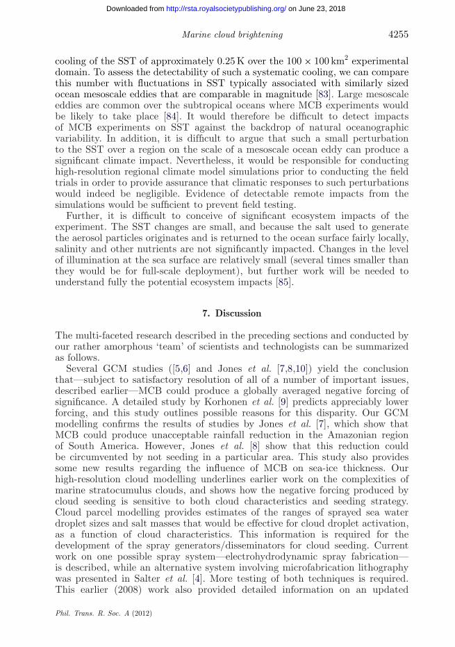
Marine cloud brightening 4255
cooling of the SST of approximately 0.25 K over the 100 × 100 km2 experimentaldomain. To assess the detectability of such a systematic cooling, we can comparethis number with fluctuations in SST typically associated with similarly sizedocean mesoscale eddies that are comparable in magnitude [83]. Large mesoscaleeddies are common over the subtropical oceans where MCB experiments wouldbe likely to take place [84]. It would therefore be difficult to detect impactsof MCB experiments on SST against the backdrop of natural oceanographicvariability. In addition, it is difficult to argue that such a small perturbationto the SST over a region on the scale of a mesoscale ocean eddy can produce asignificant climate impact. Nevertheless, it would be responsible for conductinghigh-resolution regional climate model simulations prior to conducting the fieldtrials in order to provide assurance that climatic responses to such perturbationswould indeed be negligible. Evidence of detectable remote impacts from thesimulations would be sufficient to prevent field testing.
Further, it is difficult to conceive of significant ecosystem impacts of theexperiment. The SST changes are small, and because the salt used to generatethe aerosol particles originates and is returned to the ocean surface fairly locally,salinity and other nutrients are not significantly impacted. Changes in the levelof illumination at the sea surface are relatively small (several times smaller thanthey would be for full-scale deployment), but further work will be needed tounderstand fully the potential ecosystem impacts [85].
7. Discussion
The multi-faceted research described in the preceding sections and conducted byour rather amorphous ‘team’ of scientists and technologists can be summarizedas follows.
Several GCM studies ([5,6] and Jones et al. [7,8,10]) yield the conclusionthat—subject to satisfactory resolution of all of a number of important issues,described earlier—MCB could produce a globally averaged negative forcing ofsignificance. A detailed study by Korhonen et al. [9] predicts appreciably lowerforcing, and this study outlines possible reasons for this disparity. Our GCMmodelling confirms the results of studies by Jones et al. [7], which show thatMCB could produce unacceptable rainfall reduction in the Amazonian regionof South America. However, Jones et al. [8] show that this reduction couldbe circumvented by not seeding in a particular area. This study also providessome new results regarding the influence of MCB on sea-ice thickness. Ourhigh-resolution cloud modelling underlines earlier work on the complexities ofmarine stratocumulus clouds, and shows how the negative forcing produced bycloud seeding is sensitive to both cloud characteristics and seeding strategy.Cloud parcel modelling provides estimates of the ranges of sprayed sea waterdroplet sizes and salt masses that would be effective for cloud droplet activation,as a function of cloud characteristics. This information is required for thedevelopment of the spray generators/disseminators for cloud seeding. Currentwork on one possible spray system—electrohydrodynamic spray fabrication—is described, while an alternative system involving microfabrication lithographywas presented in Salter et al. [4]. More testing of both techniques is required.This earlier (2008) work also provided detailed information on an updated
Phil. Trans. R. Soc. A (2012)
on June 23, 2018http://rsta.royalsocietypublishing.org/Downloaded from

4256 J. Latham et al.
version of unmanned, satellite-guided, wind-powered Flettner-rotor vessels, whichcould be the vehicles from which the spray droplets would be disseminated,if MCB was ever to be deployed. Here, we present CFD studies of possibleinstabilities in Flettner rotors. Finally, we summarize current thinking regardinga possible three-stage quantitative field study of MCB, designed to determinewhether cloud seeding with sea water aerosol can increase cloud albedo, and,if so, to what degree and under what circumstances. This study—which weenvisage would be performed on a spatial scale of about 100 × 100 km2, andis not designed to examine possible effects on climate—should also yield usefulfundamental information on these climatologically important clouds. As alreadystated, deployment of MCB should never occur unless approved by the relevantinternational authority, and shown, via intensive modelling studies, to have nolikelihood of significant adverse consequences.
It is unclear whether deployment of the MCB geoengineering technique wouldbe warranted, even if the climate-change problem reached such a drastic stagethat some form of intervention was deemed to be required. GCM modellingby three independent groups, using three different models [6,7,10], indicatesthat, if it functioned as assumed in the modelling, it could—roughly—stabilizethe Earth’s average surface temperature and maintain current levels of polarsea-ice cover at approximately current values for some decades, at least upto the carbon dioxide-doubling point, where the required negative forcing forfull compensation is approximately −3.7 W m−2. The computations of Korhonenet al. [9], discussed in §2, yield significantly lower values of negative forcing. Thisdisparity may result from the usage of appreciably different values of natural(no-seeding) CDNCs, N0 (see §§1 and 2) or possibly the vertical velocity fieldvalues used in their simulations were too small. In practice, it may be possibleto reconcile these disparate results by increasing the dissemination rate of seawater aerosol assumed in the Korhonen study—which we believe would be feasibletechnologically. However, as discussed in §4, marine stratocumulus clouds aremuch more complex than has been implicitly assumed in this modelling, andconsiderably more fundamental research into these clouds is required before wecan establish whether our assumptions are justified to an acceptable degree. Also,we have not yet established—for all situations of interest—quantitative values forthe fraction of spray droplets generated at or near the ocean surface that enterthe bases of the clouds above. Nor have we succeeded to date in developing a seawater spray-production system that meets our requirements as to droplet size andspray rate. Finally, we have not yet thoroughly examined the (possibly adverse)ramifications of deployment of the technique. No case for deployment would existunless it was established that all such deleterious effects of significance couldbe remedied. We need constantly to keep in mind that, while some areas maybenefit from MCB geoengineering, there may well be regions where the responseis significantly detrimental. If so, and if this situation could not be corrected,deployment of MCB would not be justified.
Two advantages of MCB, in principle, are that (i) the sprays could be switchedoff immediately, with essentially all of the sea water droplets returning to theocean within a few days, and (ii) because, for some decades, not all suitable cloudswould need to be seeded in order to produce sufficient negative forcing to balancethe carbon dioxide increase, there exists, in principle, flexibility to confine theseeding to selected cloudy areas which produce no adverse consequences or reduce
Phil. Trans. R. Soc. A (2012)
on June 23, 2018http://rsta.royalsocietypublishing.org/Downloaded from
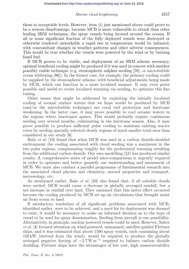
Marine cloud brightening 4257
them to acceptable levels. However, item (i) just mentioned above could prove tobe a serious disadvantage, because MCB is more vulnerable to attack than otherleading SRM techniques, the spray vessels being located around the oceans. Ifall or some significant fraction of the fully deployed vessels were destroyed orotherwise rendered unworkable a rapid rise in temperature would be initiated,with concomitant changes in weather patterns and other adverse consequences.This would be true whether the vessels were powered by the wind or by burningfossil fuel.
If MCB proves to be viable, and deployment of an SRM scheme necessary,optimal beneficial cooling might be produced if it was used in concert with anotherpossibly viable technique (e.g. stratospheric sulphur seeding [59], or microbubbleocean whitening [86]). In the former case, for example, the primary cooling couldbe supplied by the stratospheric scheme, with beneficial adjustments being madeby MCB, which can function in a more localized manner. It may even provepossible and useful to create localized warming via seeding, to optimize this finetuning.
Other issues that might be addressed by exploiting the initially localizedcooling of oceanic surface waters that we hope would be produced by MCB(and/or the microbubble technique) are coral reef protection and hurricaneweakening. In the latter case, it may prove possible to cool oceanic waters inthe regions where hurricanes spawn. This would probably require continuousseeding over several months, culminating in the hurricane season. Also, it mayprove possible to produce sufficient polar cooling to maintain existing sea-icecover by seeding specially selected cloudy regions of much smaller total area thanconsidered in our study [6].
Bala et al. [10] found that when MCB was used in a carbon dioxide-doubledenvironment the cooling associated with cloud seeding was a maximum in thetwo polar regions, compensating roughly for the preferential warming resultingfrom the additional carbon dioxide. Our own modelling (§2) has produced similarresults. A comprehensive series of model inter-comparisons is urgently requiredin order to optimize and better quantify our understanding and assessment ofMCB. We must also conduct a parallel programme of fundamental research intothe associated cloud physics and chemistry, aerosol properties and transport,meteorology, etc.
As mentioned earlier, Bala et al. [10] also found that, if all suitable cloudswere seeded, MCB would cause a decrease in globally averaged rainfall, but anet increase in rainfall over land. They surmised that this latter effect occurredbecause the cooling produced by MCB set up air circulations that brought moistair from ocean to land.
If satisfactory resolution of all significant problems associated with MCB,identified earlier, were to be achieved, and a need for its deployment was deemedto exist, it would be necessary to make an informed decision as to the type ofvessel to be used for spray dissemination. Seeding from aircraft is one possibility.Alternatively, in principle, nuclear-powered vessels could be used. However, Salteret al. [4] focused attention on wind-powered, unmanned, satellite-guided Flettnerships, and it was estimated that about 1500 spray vessels, each consuming about150 kW (derived from the wind), would be required to produce the globallyaveraged negative forcing of −3.7 W m−2 required to balance carbon dioxidedoubling. Flettner ships have the advantages of low cost, high manoeuvrability
Phil. Trans. R. Soc. A (2012)
on June 23, 2018http://rsta.royalsocietypublishing.org/Downloaded from

4258 J. Latham et al.
and low carbon footprint. A conventionally, powered ship might consume about1 MW; so, for both types of vessel, the ratio of the rate of planetary radiativeloss to required operational power is very large (in the range from 105 to 107). Itfollows that considerations of energy efficiency, desirable though that is, shouldnot dictate the selection of type of spray vessel. Latham et al. [5] pointed out thatthe main reason that this ratio is so high for MCB is that Nature provides theenergy required for the increase of surface area of newly activated cloud dropletsby four or five orders of magnitude as they ascend to cloud top and reflect sunlight.
The earlier mentioned arguments are based on the assumption that currentGCM modelling is reasonably accurate. However, if it transpires that estimatedalbedo change/droplet flux ratio values are seriously inflated because, forexample, of significant overestimation of the fraction of disseminated sea waterparticles that rise into the clouds, this issue would need to be reassessed. Otherfactors then to consider include the levels of pollution produced by spray vesselsand the energy they consume. It is also to be noted that, during the decadesleading to carbon dioxide doubling, the amount of negative forcing required ofMCB would be correspondingly less, as would the emissions (which would bevery low for wind-powered Flettner vessels). Definitive statements on these issuesmust wait on further research, on all fronts covered in this article.
We are grateful for the detailed and extremely helpful comments provided by the two reviewersof this study. We are deeply appreciative of the important role played by Kelly Wanser in thedevelopment of our research activity. We are grateful to Graham Feingold for helpful comments.We are grateful for the use of NERC, NCAS, HECToR supercomputer resources. Support forelements of this research was provided by the Fund for Innovative Climate and Energy Research,FICER, at the University of Calgary. This does not constitute endorsement of deployment inany form of cloud albedo modification by the funding agency. Part of this work was performedat the Stanford Nanofabrication Facility, supported by National Science Foundation grant no.ECS-9731293.
References
1 Latham, J. 1990 Control of global warming? Nature 347, 339–340. (doi:10.1038/347339b0)2 Latham, J. 2002 Amelioration of global warming by controlled enhancement of the albedo
and longevity of low-level maritime clouds. Atmos. Sci. Lett. 3, 52–58. (doi:10.1006/asle.2002.0099)
3 Bower, K., Choularton, T., Latham, J., Sahraei, J. & Salter, S. 2006 Computational assessmentof a proposed technique for global warming mitigation via albedo enhancement of marinestratocumulus clouds. Atmos. Res. 82, 328–336. (doi:10.1016/j.atmosres.2005.11.013)
4 Salter, S., Sortino, G. & Latham, J. 2008 Sea-going hardware for the cloud albedo method ofreversing global warming. Phil. Trans. R. Soc. A 366, 3989–4006. (doi:10.1098/rsta.2008.0136)
5 Latham, J., Rasch, P., Chen, C.-C., Kettles, L., Gadian, A., Gettelman, A., Morrison, H., Bower,K. & Choularton, T. 2008 Global temperature stabilization via controlled albedo enhancementof low-level maritime clouds. Phil. Trans. R. Soc. A 366, 3969–3987. (doi:10.1098/rsta.2008.0137)
6 Rasch, P., Latham, J. & Chen, C.-C. 2009 Geoengineering by cloud seeding: influence on seaice and climate system. Environ. Res. Lett, 4, 045112. (doi:10.1088/1748-9326/4/4/045112)
7 Jones, A., Hayward, J. & Boucher, O. 2009 Climate impacts of geoengineering marinestratocumulus clouds. J. Geophys. Res. 114, D10106. (doi:10.1029/2008JD011450)
8 Jones, A., Hayward, J. & Boucher, O. 2011 A comparison of the climate impacts ofgeoengineering by stratospheric SO2 injection and by brightening of marine stratocumulusclouds. Atmos. Sci. Lett. 12, 176–183. (doi:10.1002/asl.291)
Phil. Trans. R. Soc. A (2012)
on June 23, 2018http://rsta.royalsocietypublishing.org/Downloaded from

Marine cloud brightening 4259
9 Korhonen, H., Carslaw, K. S. & Romakkaniemi, S. 2010 Enhancement of marine cloud albedovia controlled sea spray injections: a global model study of the influence of emission rates,microphysics and transport. Atmos. Chem. Phys. Discuss. 10, 735–761. (doi:10.5194/acpd-10-735-2010)
10 Bala, G., Caldreia, K., Nemani, R., Cao, L., Ban-Weiss, G. & Shin, H.-J. 2010 Albedoenhancement of marine cloud to counteract global warming: impacts on the hydrological cycle.Clim. Dyn. 37, 915–931. (doi:10.1007/s00382-010-0868-1)
11 Byun, D., Lee, Y., Tran, S. B. Q., Nugyen, V. D., Lee, S., Kim, S., Inamdar, N., Park, B. &Bau, H. 2008 Electrospray on super hydrophobic nozzles treated with argon and oxygen plasma.Appl. Phys. Lett. 92, 093507. (doi:10.1063/1.2840725)
12 Twomey, S. 1977 Influence of pollution on the short-wave albedo of clouds. J. Atmos. Sci. 34,1149–1152. (doi:10.1175/1520-0469(1977)034<1149:TIOPOT>2.0.CO;2)
13 Albrecht, B. 1989 Aerosols, cloud microphysics, and fractional cloudiness. Science 245,1227–1230. (doi:10.1126/science.245.4923.1227)
14 Lohmann, U. & Feichter, J. 2005 Global indirect aerosol effects: a review. Atmos. Chem. Phys.5, 715–737. (doi:10.5194/acp-5-715-2005)
15 Stevens, B. & Feingold, G. 2009 Untangling aerosol effects on clouds and precipitation in abuffered system. Nature 461, 607–613. (doi:10.1038/nature08281)
16 Wang, H., Rasch, P. & Feingold, G. 2011 Manipulating marine stratocumulus cloudamount and albedo: a process-modelling study of aerosol-cloud-precipitation interactionsin response to injection of cloud condensation nuclei. Atmos. Chem. Phys. 11, 4237–4239.(doi:10.5194/acp-11-4237-2011)
17 Bennartz, R. 2007 Global assessment of marine boundary layer cloud droplet numberconcentration from satellite. J. Geophys. Res. Atmos. 112(D2), D02201. (doi:10.1029/2006JD007547)
18 Wood, R. et al. 2011 The VAMOS Ocean-Cloud-Atmosphere-Land Study Regional Experiment(VOCALS-REx): goals, platforms, and field operations. Atmos. Chem. Phys. 11, 627–654.(doi:10.5194/acp-11-627-2011)
19 Martin, G. M., Ringer, M. A., Pope, V. D., Jones, A., Dearden, C. & Hinton, T. J. 2006The physical properties of the atmosphere in the new Hadley centre global environmentalmodel (HadGEM1). I. Model description and global climatology. J. Clim. 19, 1274–1301.(doi:10.1175/JCLI3636.1)
20 Randall, D. A. et al. 2007 Climate models and their evaluation. In Climate Change 2007: Thephysical science basis. Contribution of Working Group I to the Fourth Assessment Report ofthe Intergovernmental Panel on Climate Change (eds S. Solomon, D. Qin, M. Manning, Z.Chen, M. Marquis, K. B. Averyt, M. Tignor & H. L. Miller). Cambridge, UK: CambridgeUniversity Press.
21 Xie, P. & Arkin, P.A. 1997 Global precipitation: a 17-year monthly analysis based on gaugeobservations, satellite estimates, and numerical model outputs. Bull. Am. Meteor. Soc. 78,2539–2558. (doi:10.1175/1520-0477(1997)078<2539:GPAYMA>2.0.CO;2)
22 Winston, M. 2011 Do climate models underestimate the sensitivity of northern hemisphere seaice cover? J. Clim. 24, 3924–3934. (doi:10.1175/2011JCLI4146.1)
23 Abel, S. J., Walters, D. N. & Allen, G. 2010 Evaluation of stratocumulus cloud prediction inthe Met Office forecast model during VOCALS-Rex. Atmos. Chem. Phys. Discuss. 10, 16 797–16 835. (doi:10.5194/acpd-10-16797-2010)
24 Wyant, M. C. et al. 2010 The PreVOCA experiment: modeling the lower troposphere in thesoutheast Pacific. Atmos. Chem. Phys. 10, 4453–5010. (doi:10.5194/acp-10–4757–2010)
25 Bony, S. & Dufresne, J.-L. 2005 Marine boundary layer clouds at the heart of tropicalcloud feedback uncertainties in climate models. Geophys. Res. Lett. 32, L20806. (doi:10.1029/2005GL023851)
26 Twomey, S. 1974 Pollution and the planetary albedo. Atmos. Environ. 8, 1251–1256.(doi:10.1016/0004-6981(74)90004-3)
27 Ackerman, A. S., Kirkpatrick, M. P., Stevens, D. E. & Toon, O. B. 2004 The impact ofhumidity above stratiform clouds on indirect aerosol climate forcing. Nature 432, 1014–1017.(doi:10.1038/nature03174)
Phil. Trans. R. Soc. A (2012)
on June 23, 2018http://rsta.royalsocietypublishing.org/Downloaded from

4260 J. Latham et al.
28 Wood, R. 2007 Cancellation of aerosol indirect effects in marine stratocumulus through cloudthinning. J. Atmos. Sci. 64, 2657–2669. (doi:10.1175/jas3942.1)
29 Ackerman, A. S. et al. 2009 Large-eddy simulations of a drizzling, stratocumulus-topped marineboundary layer. Mon. Weather Rev. 137, 1083–1110. (doi:10.1175/2008MWR2582.1)
30 Leon, D. C., Wang, Z. & Liu, D. 2008 Climatology of drizzle in marine boundary layer cloudsbased on 1 year of data from cloudsat and cloud–aerosol lidar and infrared pathfinder satelliteobservations (CALIPSO). J. Geophys. Res. 113, D00A14. (doi:10.1029/2008JD009835)
31 Kubar, T.L., Hartmann, D. L. & Wood, R. 2009 Understanding the importance of microphysicsand macrophysics for warm rain in marine low clouds. I. Satellite observations. J. Atmos. Sci.66, 2953–2972. (doi:10.1175/2009JAS3071.1)
32 Bretherton, C. S., Wood, R., George, R. C., Leon, D., Allen, G. & Zheng, X. 2010Southeast Pacific stratocumulus clouds, precipitation and boundary layer structure sampledalong 20 S during VOCALS-REx. Atmos. Chem. Phys. Discuss. 10, 15 921–15 962.(doi:10.5194/acpd-10-15921-2010)
33 Wang, H. & Feingold, G. 2009 Modelling open cellular structures and drizzle in marinestratocumulus. I. Impact of drizzle on the formation and evolution of open cells. J. Atmos.Sci. 66, 3237–3256. (doi:10.1175/2009JAS3022.1)
34 Wang, H. & Feingold, G. 2009 Modelling open cellular structures and drizzle in marinestratocumulus. II. The microphysics and dynamics of the boundary region between open andclosed cells. J. Atmos. Sci. 66, 3257–3275. (doi:10.1175/2009JAS3120.1)
35 Feingold, G., Koren, I., Wang, H., Xue, H. & Brewer, W. A. 2010 Precipitation-generatedoscillations in open cellular cloud fields. Nature 466, 849–852. (doi:10.1038/nature09314)
36 Wang, S. P., Wang, Q. & Feingold, G. 2003 Turbulence, condensation, and liquid watertransport in numerically simulated nonprecipitating stratocumulus clouds. J. Atmos. Sci. 60,262–278. (doi:10.1175/1520-0469(2003)060<0262:TCALWT>2.0.CO;2)
37 Bretherton, C. S., Blossey, P. N. & Uchida, J. 2007 Cloud droplet sedimentation, entrainmentefficiency, and subtropical stratocumulus albedo. Geophys. Res. Lett. 34, L03813. (doi:10.1029/2006GL027648)
38 Rosenfeld, D., Kaufman, Y. J. & Koren, I. 2006 Switching cloud cover and dynamical regimesfrom open to closed Benard cells in response to the suppression of precipitation by aerosols.Atmos. Chem. Phys. 6, 2503–2511. (doi:10.5194/acp-6-2503-2006)
39 Connolly, P., Möhler, O., Field, P. R., Saathoff, H., Burgess, R., Choularton, T. & Gallagher,M. 2009 Studies of heterogeneous freezing by three different desert dust samples. Atmos. Chem.Phys. 9, 2805–2824. (doi:10.5194/acp-9-2805-2009)
40 Topping, D., McFiggans, G. B. & Coe, H. 2005 A curved multi-component aerosolhygroscopicity model framework. I. Inorganic compounds. Atmos. Chem. Phys. 5, 1205–1222.(doi:10.5194/acp-5-1205-2005)
41 Jacobson, M. 2005 Fundamentals of atmospheric modelling, 2nd edn. New York, NY: CambridgeUniversity Press.
42 Seinfeld, J. & Pandis, S. 2006 Atmospheric chemistry and physics: from air pollution to climatechange, 2nd edn. Hoboken, NJ: Wiley-Blackwell.
43 Taylor, G. 1964 Disintegration of water drops in an electric field. Proc. R. Soc. Lond. A 280,383–397. (doi:10.1098/rspa.1964.0151)
44 De la Mora, J. F. 2007 The fluid dynamics of Taylor cones. Annu. Rev. Fluid Mech. 39, 217–243.(doi:10.1146/annurev.fluid.39.050905.110159)
45 Gañán-Calvo, A. M. & Montanero, J. M. 2009 Revision of capillary cone-jet physics:electrospray and flow focusing. Phys. Rev. E 79, 066305. (doi:10.1103/PhysRevE.79.066305)Publisher’s note in Phys. Rev. E 2009 79, 069905. (doi:10.1103/PhysRevE.79.069905)
46 Crowley, J. M. 1977 Role of Joule heating in the electrostatic spraying of liquids. J. Appl. Phys.48, 145–147. (doi:10.1063/1.323299)
47 Deng, W., Waits, C. M., Morgan, B. & Gomez, A. 2009 Compact multiplexing of monodisperseelectrosprays. J. Aerosol Sci. 40, 907–918. (doi:10.1016/j.jaerosci.2009.07.002)
48 Lozano, P., Martínez-Sánchez, M. & Lopez-Urdiales, J. M. 2004 Electrospray emissionfrom non-wetting flat dielectric surfaces. J. Colloid Interface Sci. 276, 392–399.(doi:10.1016/j.jcis.2004.04.017)
Phil. Trans. R. Soc. A (2012)
on June 23, 2018http://rsta.royalsocietypublishing.org/Downloaded from

Marine cloud brightening 4261
49 Bocanegra, R., Galán, D., Márquez, M., Loscertales, I. G. & Barrero, A. 2005 Multipleelectrosprays emitted from an array of holes. J. Aerosol Sci. 36, 1387–1399. (doi:10.1016/j.jaerosci.2005.04.003)
50 Reverchon, E. & Spada, A. 2004 Crystalline micro-particles of controlled size produced bysuper-critical atomization. Ind. Eng. Chem. Res. 43, 1460–1465. (doi:10.1021/ie034111t)
51 Gadian, A., Blyth, A., Latham, J., Salter, S. & Stevens, L. 2009 Whitening theclouds. Planet Earth Online, 14 December 2009. See http://planetearth.nerc.ac.uk/features/story.aspx?id=584.
52 Thom, A. 1934 On the effects of discs on the air forces on a rotating cylinder. AeronauticalResearch Committee Report and Memoranda issue 1623. London, UK: HM Stationery Office.
53 Mittal, S. and Kumar, B. 2003 Flow past a rotating cylinder. J. Fluid Mech. 476, 302–334.(doi:10.1017/S0022112002002938)
54 Lien, F.-S. & Leschziner, M. A. 1994 A general non-orthogonal finite-volume algorithm forturbulent flow at all speeds incorporating second-moment closure. Part 1. Numerical implemen-tation. Comp. Meth. Appl. Mech. Eng. 114, 123–148. (doi:10.1016/0045-7825(94)90165-1)
55 Craft, T. J., Gerasimov, A. V., Iacovides, H. & Launder, B. E. 2004 The negatively buoyantwall jet: the performance of options in RANS modelling. Int. J. Heat Fluid Flow 25, 809–823.(doi:10.1016/j.ijheatfluidflow.2004.05.003)
56 Reid, E. G. 1924 Tests of rotating cylinders. National Advisory Committee TechnicalNote no. 209. Langley Memorial Aeronautical Laboratory, Hampto, VA. Seehttp://naca.central.cranfield.ac.uk/reports/1924/naca-tn-209.pdf.
57 Craft, T. J., Iacovides, H. & Launder, B. E. 2010 Computational modelling of Flettner rotorperformance with and without Thom discs. In Proc. 8th Int. ERCOFTAC Symp. on EngineeringTurbulence Modelling and Measurements, ETMM8, Marseilles, France, 8–10 June 2010,pp. 152–157.
58 Robock, A., Bunzl, M., Kravitz, B., Georgiy, L. & Stenchikov, G. L. 2010 A test forgeoengineering? Science 327, 530–531. (doi: 10.1126/science.1186237)
59 Crutzen, P. J. 2006 Albedo enhancement by stratospheric sulfur injections: a contribution toresolve a policy dilemma. Clim. Change 77, 211–219. (doi:10.1007/s10584-006-9101-y)
60 Royal Society 2009 Geoengineering the climate: science, governance and uncertainty. SciencePolicy Report 10/09. London, UK: Royal Society.
61 Minnis, P., Harrison, E. F., Stowe, L. L., Gibson, G. G., Denn, F. M., Doelling, D. R. &Smith Jr, W. L. 1993 Radiative climate forcing by the Mount Pinatubo eruption. Science 259,1411–1415. (doi:10.1126/science.259.5100.1411)
62 McCormick, M. P., Thomason, L. W. & Trepte, C. R. 1995 Atmospheric effects of the MtPinatubo eruption. Nature 373, 399–404. (doi:10.1038/373399a0)
63 IPCC. 2007 Climate Change 2007: The physical science basis. Contribution of Working Group Ito the Fourth Assessment Report of the Intergovernmental Panel on Climate Change (edsS. Solomon, D. Qin, M. Manning, Z. Chen, M. Marquis, K. B. Averyt, M. Tignor & H. L.Miller). Cambridge, UK: Cambridge University Press.
64 Isaksen, I. S. A. et al. 2009 Atmospheric composition change: climate–chemistry interactions.Atmos. Environ. 43, 5138–5192. (doi:10.1016/j.atmosenv.2009.08.003)
65 Johnson, D. W. et al. 2000 Observations of the evolution of the aerosol, cloud and boundary-layer characteristics during the 1st ACE-2 Lagrangian experiment. Tellus B 52, 348–374.(doi:10.1034/j.1600-0889.2000.00087.x)
66 Stevens, B. et al. 2003 Dynamics and chemistry of marine stratocumulus: DYCOMS II. Bull.Am. Meteorol. Soc. 84, 579–593. (doi:10.1175/BAMS-84-5-579)
67 Russell, L. M. et al. 1999 Aerosol dynamics in ship tracks. J. Geophys. Res. 104, 31 077–31 095.68 Boyd, P. W. et al. 2007 Mesoscale iron enrichment experiments 1993–2005: synthesis and future
directions. Science 315, 612–617. (doi:10.1126/science.1131669)69 Lampitt, R. S. et al. 2008 Ocean fertilization: a potential means of geoengineering? Phil. Trans.
R. Soc. A 366, 3919–3945. (doi:10.1098/rsta.2008.0139)70 Rayner 2010 The regulation of geoengineering. See http://www.sbs.ox.ac.uk/centres/insis/
news/Pages/regulation-geoengineering.aspx.
Phil. Trans. R. Soc. A (2012)
on June 23, 2018http://rsta.royalsocietypublishing.org/Downloaded from

4262 J. Latham et al.
71 Morgan, G. & Ricke, K. 2010 Cooling the earth through solar radiation management. Geneva,Switzerland: International Risk Governance Council.
72 Durkee, P. A., Chartier, R. E., Brown, A., Trehubenko, E. J., Rogerson, S. D., Skupniewicz,C., Nielsen, K. E., Platnick, S. & King, M. D. 2000 Composite ship track characteristics.J. Atmos. Sci. 57, 2543–2553. (doi:10.1175/1520-0469(2000)057<2542:CSTC>2.0.CO;2)
73 Conover, J. H. 1966 Anomalous cloud lines. J. Atmos. Sci. 23, 778–785. (doi:10.1175/1520-0469(1966)023<0778:ACL>2.0.CO;2)
74 Coakley Jr, J. A., Bernstein, R. L. & Durkee, P. A. 1987 Effect of ship-stack effluents on cloudreflectivity. Science 237, 1020–1022. (doi:10.1126/science.237.4818.1020)
75 Coakley, J. A. et al. 2000 The appearance and disappearance of ship tracks on large spatialscales. J. Atmos. Sci. 57, 2765–2778. (doi:10.1175/1520-0469(2000)057<2765:TAADOS>2.0.CO;2)
76 Hobbs, P. V. et al. 2000 Emissions from ships with respect to their effects on clouds. J. Atmos.Sci., 57, 2570–2590. (doi:10.1175/1520-0469(2000)057<2570:EFSWRT>2.0.CO;2)
77 Durkee, P. A., Noone, K. J. & Bluth, R. T. 2000 The Monterey area ship track experiment.J. Atmos. Sci. 57, 2523–2541. (doi:10.1175/1520-0469(2000)057<2523:TMASTE>2.0.CO;2)
78 Heffter, J. L. 1965 The variation of horizontal diffusion parameters with time for travelperiods of one hour or longer. J. Appl. Meteor. 4, 153–156. (doi:10.1175/1520-0450(1965)004<0153:TVOHDP>2.0.CO;2)
79 Coakley, J. A. & Walsh, C. D. 2002 Limits to the aerosol indirect radiative effect derivedfrom observations of ship tracks. J. Atmos. Sci. 59, 668–680. (doi:10.1175/1520-0469(2002)059<0668:LTTAIR>2.0.CO;2)
80 Platnick, S. & Twomey, S. 1994 Determining the susceptibility of cloud albedo to changes indroplet concentration with the advanced very high resolution radiometer. J. Appl. Meteorol.33, 334–347. (doi:10.1175/1520-0450(1994)033<0334:DTSOCA>2.0.CO;2)
81 Oreopoulos, L. & Platnick, S. 2008 Radiative susceptibility of cloudy atmospheres to dropletnumber perturbations. II. Global analysis from MODIS. J. Geophys. Res. 113, D14S21.(doi:10.1029/2007JD009655)
82 de Boyer Montégut, C., Madec, G., Fischer, A. S., Lazar, A. & Iudicone, D. 2004 Mixed layerdepth over the global ocean: An examination of profile data and a profile-based climatology.J. Geophys. Res. 109, C12003. (doi:10.1029/2004JC002378)
83 Chaigneau, A., Le Texier, M., Eldin, G., Grados, C. & Pizarro, O. 2011 Vertical structure ofmesoscale eddies in the eastern South Pacific Ocean: a composite analysis from altimetry andArgo profiling floats. J. Geophys. Res. 116, C11025. (doi:10.1029/2011JC007134)
84 Chelton, D. B., Schlax, M. G., Samelson, R. M. & de Szoeke, R. A. 2007 Global observationsof large oceanic eddies. Geophys. Res. Lett. 34, L15606. (doi:10.1029/2007GL030812)
85 Russell, L. M. et al. 2012 Ecosystem impacts of geoengineering: a review for developing a scienceplan. Ambio 41, 350–369. (doi:10.1007/s13280-012-0258-5)
86 Seitz, R. 2011 Bright water: hydrosols, water conservation and climate change. Climatic Change105, 365–381.
Phil. Trans. R. Soc. A (2012)
on June 23, 2018http://rsta.royalsocietypublishing.org/Downloaded from