rsta.royalsocietypublishing.org

ReviewCite this article: Schlamminger S, Pixley RE,Nolting F, Schurr J, Straumann U. 2014Reflections on a measurement of thegravitational constant using a beam balanceand 13 tons of mercury. Phil. Trans. R. Soc. A372: 20140027.http://dx.doi.org/10.1098/rsta.2014.0027

One contribution of 13 to a Theo MurphyMeeting Issue ‘The Newtonian constant ofgravitation, a constant too difficult tomeasure?’

Subject Areas:mechanics

Keywords:gravitational constant, mass comparator,mercury

Author for correspondence:S. Schlammingere-mail: stephan.schlamminger@nist.gov

Reflections on a measurementof the gravitational constantusing a beam balance and 13tons of mercuryS. Schlamminger1, R. E. Pixley2, F. Nolting3, J. Schurr4

and U. Straumann2

1National Institute of Standards and Technology, Gaithersburg,MD 20899, USA2Physik-Institut der Universität Zürich, 8057 Zürich, Switzerland3Paul Scherrer Institut, 5232 Villigen, Switzerland4Physikalisch Technische Bundesanstalt, 38116 Braunschweig,Germany

In 2006, a final result of a measurement of the gravi-tational constant G performed by researchers at theUniversity of Zürich, Switzerland, was published. Avalue of G = 6.674252(122) × 10−11 m3 kg−1 s−2 wasobtained after an experimental effort that lastedover one decade. Here, we briefly summarizethe measurement and discuss the strengths andweaknesses of this approach.

1. IntroductionThe existence of the Zürich G experiment is due to anarticle published in 1986 by Fischbach et al. [1] analysingold data collected by von Eötvös et al. [2] to test theuniversality of free fall. A deviation was found in theintermediate-range (about 200 m) coupling, giving rise tothe so-called fifth force. The existence of such a fifth forceat the strength conjectured in [1] was quickly found to bein error [3]. However, the article by Fischbach et al. starteda renaissance of gravity experiments at universitiesworldwide. Walter Kündig at the University of Zürich,Switzerland, started an experiment aimed at measuringthe gravitational attraction between water in a storagelake (Gigerwald Lake) and two masses suspended froma balance [4]. The experiment was conducted in twodifferent configurations. First, the test masses (TMs) werevertically separated by 63 m, and later by 104 m. Themagnitude of the gravitational attraction was measured

2014 The Author(s) Published by the Royal Society. All rights reserved.

on August 12, 2018http://rsta.royalsocietypublishing.org/Downloaded from

2

rsta.royalsocietypublishing.orgPhil.Trans.R.Soc.A372:20140027

.........................................................

as the water level varied seasonally over the course of several years. As a result of the experiment,two measurements of G for an interaction range of 88 m and 112 m were obtained with relativestandard uncertainties of 1 × 10−3 and 7 × 10−4, respectively [5]. The results were consistentwith each other and consistent with the value of G from laboratory determinations. Even today,20 years after this experiment, its results place the most stringent limit on a possible violationof the inverse square law at distances ranging from 10 to 100 m. The largest contribution tothe uncertainty of each result came from the ambiguous mass distribution of the lake. It wasunclear how far the lake water penetrated the shore, which is composed mostly of scree. It wasimmediately recognized that one could use the same method for a precise determination of thegravitational constant if only one had a better defined lake.

From this line of thinking, the concept of measuring G in the laboratory was conceived and thedesign of the experiment started in 1994. Conceptually, the experiment is similar to the Gigerwaldexperiment with one difference: the ‘lake’ was confined to two well-characterized stainless-steelvessels each holding 500 litres of liquid. In a first experiment, water was used; later, the water wasreplaced with mercury, yielding a much larger signal.

The Zürich big G experiment ended officially in 2006, when a final report [6] on the experimentwas published. The relevant details of the experiment have been summarized in the final report,two theses [7,8] and several shorter reports [9–14].

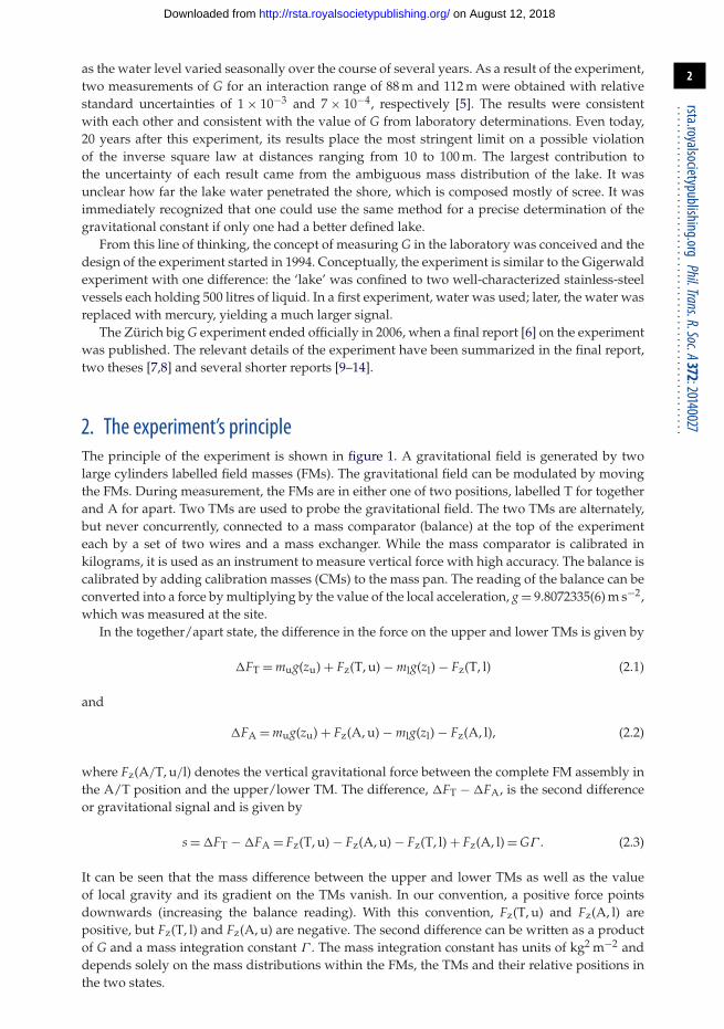
2. The experiment’s principleThe principle of the experiment is shown in figure 1. A gravitational field is generated by twolarge cylinders labelled field masses (FMs). The gravitational field can be modulated by movingthe FMs. During measurement, the FMs are in either one of two positions, labelled T for togetherand A for apart. Two TMs are used to probe the gravitational field. The two TMs are alternately,but never concurrently, connected to a mass comparator (balance) at the top of the experimenteach by a set of two wires and a mass exchanger. While the mass comparator is calibrated inkilograms, it is used as an instrument to measure vertical force with high accuracy. The balance iscalibrated by adding calibration masses (CMs) to the mass pan. The reading of the balance can beconverted into a force by multiplying by the value of the local acceleration, g = 9.8072335(6) m s−2,which was measured at the site.

In the together/apart state, the difference in the force on the upper and lower TMs is given by

�FT = mug(zu) + Fz(T, u) − mlg(zl) − Fz(T, l) (2.1)

and

�FA = mug(zu) + Fz(A, u) − mlg(zl) − Fz(A, l), (2.2)

where Fz(A/T, u/l) denotes the vertical gravitational force between the complete FM assembly inthe A/T position and the upper/lower TM. The difference, �FT − �FA, is the second differenceor gravitational signal and is given by

s = �FT − �FA = Fz(T, u) − Fz(A, u) − Fz(T, l) + Fz(A, l) = GΓ . (2.3)

It can be seen that the mass difference between the upper and lower TMs as well as the valueof local gravity and its gradient on the TMs vanish. In our convention, a positive force pointsdownwards (increasing the balance reading). With this convention, Fz(T, u) and Fz(A, l) arepositive, but Fz(T, l) and Fz(A, u) are negative. The second difference can be written as a productof G and a mass integration constant Γ . The mass integration constant has units of kg2 m−2 anddepends solely on the mass distributions within the FMs, the TMs and their relative positions inthe two states.

on August 12, 2018http://rsta.royalsocietypublishing.org/Downloaded from

3

rsta.royalsocietypublishing.orgPhil.Trans.R.Soc.A372:20140027

.........................................................1 m

2.3

m

field masses

upper test mass

lower test mass

wires

mass exchanger

balance

position T position A

–2 × 10–6 2 × 10–6

gz (N kg–1)

–2 × 10–6 2 × 10–6

gz (N kg–1)

Figure 1. Principle of the Zürich G experiment. Either of the two TMs is suspended from the balance. The FMs are either inposition T (together) or in position A (apart) as shown on the left and right side of the figure, respectively. The graphs to theside of the FMs show the vertical part of the gravitational field generated by the FMs along the symmetry axis at the centre ofthe hollow cylinders. A downward force corresponds to a positive sign. (Online version in colour.)

The size of the gravitational signal s/g ≈ 785 µg was determined with an accuracy of 14.3 ngusing a modified commercial mass comparator (Mettler Toledo AT10061). Off the shelf, thistype of mass comparator is used at national metrology institutes to compare 1 kg weights witheach other using the substitution method. The mass comparator is essentially a sophisticatedbeam balance, where a large fraction of the load on the mass pan is compensated by a fixedcounter mass. Only a small part of the gravitational force on the mass pan is compensated byan electromagnetic actuator consisting of a stationary permanent magnet system and a currentcarrying coil attached to the balance beam. The current in the coil is controlled such that thebeam remains in a constant position. The coil current is precisely measured and converted intokilograms. This value is shown on the display and can be transferred to a computer. Typically,the dynamic range of such a comparator is 24 g around 1000 g with a resolution of 100 ng. Thecomparator used in the present experiment was modified in two ways: first, the mass comparatorwas made vacuum compatible by stripping it of all plastic parts and separating the electronicsfrom the weighing cell. The electronics outside the vacuum vessel were connected to the balancevia vacuum feedthroughs. Second, the dynamic range was reduced to 4 g, thereby decreasingthe resolution to 16.7 ng by simply reducing the number of turns of the coil by a factor of six.Hence, for the same applied current to the coil, the force was reduced by a factor of six. As thecoil current was measured with the same electronics, the mass resolution decreased by a factorof six. An additional decrease to 12.5 ng was achieved by modifying the software in the balancecontroller.

1Certain commercial equipment, instruments or materials are identified in this paper in order to specify the experimentalprocedure adequately. Such identification is not intended to imply recommendation or endorsement by the National Instituteof Standards and Technology, nor is it intended to imply that the materials or equipment identified are necessarily the bestavailable for the purpose.

on August 12, 2018http://rsta.royalsocietypublishing.org/Downloaded from

4

rsta.royalsocietypublishing.orgPhil.Trans.R.Soc.A372:20140027

.........................................................

14

15

16

13

12111098

2

3

4567

1

(a)

(b)

(c)

1 m

flange

crimp tube

vacuum tube

vessel

window

100 mm

compensationvessel

bottomplate drain

700

mm

90 mm70 mm59 mm45 mm

55 mm

77m

m

25 mm

25 mm

top plate

casing

welds

10 mm

Δ 100 mm

Δ 290 mm

Δ 1046 mm

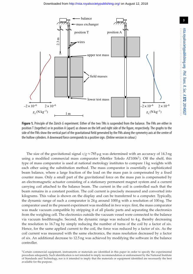
Figure 2. (a) A side view of the experiment. 1= measuring room enclosure, 2= thermally insulated chamber, 3=balance, 4= concrete walls of the pit, 5= granite plate, 6= steel girder, 7= vacuum pumps, 8= gear drive,9= motor, 10= working platform, 11= spindle, 12= steel girder of the main support, 13= upper TM, 14= FMs,15= lower TM and 16= vacuum tube. (b) A cross-sectional view of the lower TM in the vacuum tube. (c) A drawing of one ofthe vessels holding the liquid mercury.

The FMs are cylindrical vessels made from stainless steel, each with an inner volume of500 litres. Figure 2c shows a drawing of one vessel. Each vessel was filled with 6760 kg of mercury.A liquid was used to ensure a homogeneous density and mercury was chosen because of itshigh density of 13.54 g cm−3. The gravitational signal produced by the liquid is proportionalto its density. Therefore, the gravitational signal due to the mercury is 13.5 times larger thanthat of water. However, as the contribution of the stainless-steel vessels needs to be taken intoaccount, the mercury-filled vessels produce only 4.1 times the signal of the water-filled vessels.The vessels contribute about 60 µg to the signal, which is about 7.6% of the signal obtained withthe mercury-filled vessels, but 55% of the signal obtained with water-filled vessels.

The vessels were evacuated prior to filling them with mercury to avoid trapping air. Themercury was delivered in 395 flasks, each weighing about 36.5 kg (34.5 kg mercury and 2 kgdue to the steel flask). Each flask was weighed before and after its content was transferredto one of the two vessels using an evacuated transfer system. This painstakingly careful workled to a relative standard uncertainty of the mercury mass of 1.8 × 10−6 and 2.2 × 10−6 for theupper and lower vessels, respectively. The mercury for this experiment was leased, i.e. after theexperiment was dismantled in December 2002, the mercury was sent back to the supplier inSpain.

on August 12, 2018http://rsta.royalsocietypublishing.org/Downloaded from

5

rsta.royalsocietypublishing.orgPhil.Trans.R.Soc.A372:20140027

.........................................................

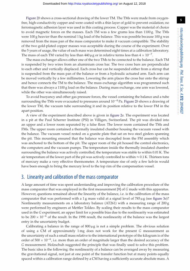
Figure 2b shows a cross-sectional drawing of the lower TM. The TMs were made from oxygen-free, high-conductivity copper and were coated with a thin layer of gold to prevent oxidation; noferromagnetic adhesion layer was used in this coating process. Copper was the material of choiceto avoid magnetic forces on the masses. Each TM was a few grams less than 1100 g. The TMswere 100 g heavier than the nominal 1 kg load of the balance. This was possible because 100 g wasremoved from the mass pan of the mass comparator to make it vacuum compatible. The stabilityof the two gold-plated copper masses was acceptable during the course of the experiment. Overthe 5 years of usage, the value of each mass was determined eight times at a calibration laboratory.The mass of each TM varied by less than 440 µg or in relative terms less than 4 × 10−7.

The mass exchanger allows either one of the two TMs to be connected to the balance. Each TMis suspended by two wires from an aluminium cross bar. The two cross bars are perpendicularto each other and vertically displaced. Each cross bar can be suspended either from a stirrup thatis suspended from the mass pan of the balance or from a hydraulic actuated arm. Each arm canbe moved vertically by a few millimetres. Lowering the arm places the cross bar onto the stirrupand hence connects the TM to the balance. The mass exchange algorithm was programmed suchthat there was always a 1100 g load on the balance. During mass exchange, one arm was lowered,while the other was simultaneously raised.

To avoid buoyancy and other gas pressure forces, the vessel containing the balance and a tubesurrounding the TMs were evacuated to pressures around 10−4 Pa. Figure 2b shows a drawing ofthe lower TM, the vacuum tube surrounding it and its position relative to the lower FM in theapart position.

A view of the experiment described above is given in figure 2a. The experiment was locatedin a pit at the Paul Scherrer Institute (PSI) in Villigen, Switzerland. The pit was divided intoan upper and a lower room separated by a false floor. The lower room contained the TMs andFMs. The upper room contained a thermally insulated chamber housing the vacuum vessel withthe balance. The vacuum vessel rested on a granite plate that sat on two steel girders spanningthe pit. This mounting ensured that the balance was decoupled from the FM assembly whichwas anchored to the bottom of the pit. The upper room of the pit housed the control electronics,the computers and the vacuum pumps. The temperature inside the thermally insulated chambersurrounding the balance was actively controlled; the temperature was stable to within 0.01 K. Theair temperature of the lower part of the pit was actively controlled to within ≈ 0.1 K. Thirteen tonsof mercury make a very effective thermometer. A temperature rise of only a few kelvin wouldhave been enough to bring the mercury level to the top rim of the compensation vessel.

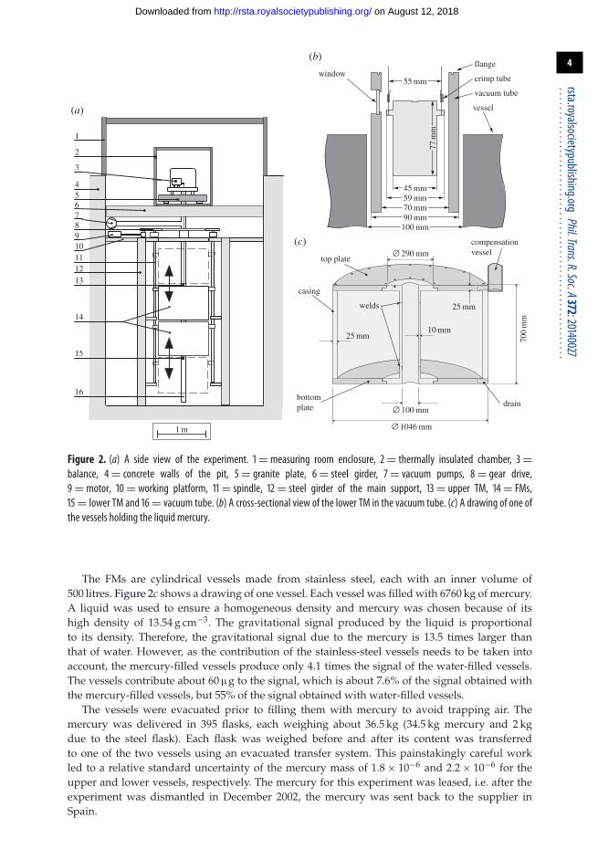
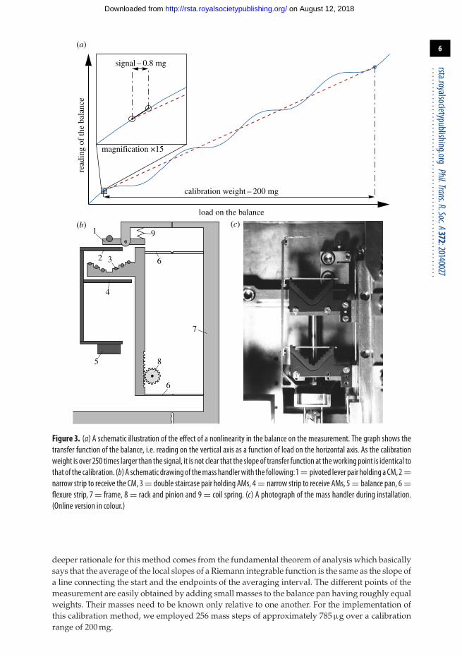
3. Linearity and calibration of the mass comparatorA large amount of time was spent understanding and improving the calibration procedure of themass comparator that was employed in the first measurement [9] of G made with this apparatus.However, questions remained about the linearity of the balance, i.e. is the calibration of the masscomparator that was performed with a 1 g mass valid at a signal level of 785 µg (see figure 3a)?Nonlinearity measurements on a laboratory balance (AT261) with a measuring range of 200 gwere performed by engineers at Mettler Toldeo. By scaling their results to the mass comparatorused in the G experiment, an upper limit for a possible bias due to the nonlinearity was estimatedto be 200 × 10−6 of the result. In the 1998 result, the nonlinearity of the balance was the largestentry in the uncertainty budget.

Calibrating a balance in the range of 800 µg is not a simple problem. The obvious solutionof using a CM of approximately 1 mg does not work for the present G measurement asthe uncertainty of such a small mass relative to the international prototype of the kilogram is of theorder of 500 × 10−6, i.e. more than an order of magnitude larger than the desired accuracy of theG measurement. Holzschuh suggested the principle that was finally used to solve this problem.The basic idea is the following: the nonlinearity of a balance can be averaged away by measuringthe gravitational signal, not just at one point of the transfer function but at many points equallyspaced within a calibration range defined by a CM having a sufficiently accurate absolute mass. A

on August 12, 2018http://rsta.royalsocietypublishing.org/Downloaded from

6

rsta.royalsocietypublishing.orgPhil.Trans.R.Soc.A372:20140027

.........................................................

load on the balance

read

ing

of th

e ba

lanc

e

calibration weight – 200 mg

magnification ×15

signal – 0.8 mg

(a)

(b) (c)1

32 6

7

4

5 8

6

9

Figure 3. (a) A schematic illustration of the effect of a nonlinearity in the balance on the measurement. The graph shows thetransfer function of the balance, i.e. reading on the vertical axis as a function of load on the horizontal axis. As the calibrationweight is over 250 times larger than the signal, it is not clear that the slope of transfer function at theworking point is identical tothat of the calibration. (b) A schematic drawingof themass handlerwith the following: 1= pivoted lever pair holding a CM, 2=narrow strip to receive the CM, 3= double staircase pair holding AMs, 4= narrow strip to receive AMs, 5= balance pan, 6=flexure strip, 7= frame, 8= rack and pinion and 9= coil spring. (c) A photograph of the mass handler during installation.(Online version in colour.)

deeper rationale for this method comes from the fundamental theorem of analysis which basicallysays that the average of the local slopes of a Riemann integrable function is the same as the slope ofa line connecting the start and the endpoints of the averaging interval. The different points of themeasurement are easily obtained by adding small masses to the balance pan having roughly equalweights. Their masses need to be known only relative to one another. For the implementation ofthis calibration method, we employed 256 mass steps of approximately 785 µg over a calibrationrange of 200 mg.

on August 12, 2018http://rsta.royalsocietypublishing.org/Downloaded from

7

rsta.royalsocietypublishing.orgPhil.Trans.R.Soc.A372:20140027

.........................................................

Although the basic principle of this method is based on equal mass steps over a calibrationrange, it is difficult to make small masses with exactly equal mass. In addition, it was notalways possible to make all mass steps due to malfunction of the auxiliary mass (AM) handler. Asomewhat more general analysis method was developed to overcome these problems. For thispurpose, a series of Legendre polynomials with an arbitrary highest order Lmax was chosen.Hence, the calibrated reading of the balance f (u) as a function of the mass u on the mass pancan be written as

f (u) =Lmax∑�=0

a�P�(ξ ), (3.1)

where P� is a Legendre polynomial of order � and ξ = 2u/umax − 1. Two constraints, f (0) = 0 andf (C) = C, reduce the number of degrees of freedom from Lmax + 1 to Lmax − 1, where C is the sumof the two CMs. Thus, the values of a0 and a1 are given by

a0 = C2

−Lmax∑

even �=2

a� and a1 = C2

−Lmax∑

odd �=3

a�. (3.2)

The remaining Lmax − 1 parameters a�, and the size of the signal s/g, were obtained by minimizing

χ2 =N∑

n=1

[f(un + s/g

) − f (un) − yn]2

σ−2n ,

where yn is the calibrated reading obtained with offset un, and σn is the statistical standarddeviation of the reading. The minimization of χ2 is straightforward. As s/g is the only nonlinearparameter, a one-parameter search for a minimum is all that is required. The a� parameters arelinear and can be solved by a trivial matrix inversion. The number of parameters required for areasonable fit can be determined from the value of χ2.

The small masses used for shifting the measuring point are referred to as AMs. Two sets ofAMs were employed. One set (AM-1) contained 16 masses with an average value of 783 µg anda standard deviation of 1.5 µg. The other set (AM-2) contained 16 masses with an average massof 16 times 783 µg and a standard deviation of 2.3 µg. With combinations of these two sets ofmasses, it is possible to have 256 approximately equal mass steps in the calibration interval from0 to 200 mg. The masses of AM-1 and AM-2 were made from stainless-steel wire with a diameterof 0.1 mm and 0.3 mm, respectively.

The device for loading the masses on the balance is shown in figure 3b. Initially, each set ofmasses rests on one of the two separately controlled double staircases bracketing a narrow metalstrip attached to the balance pan. The steps are 2 mm high and 2 mm wide. They are arranged inthe form of a ‘V’. The vertical position of each staircase is controlled by a rack and pinion devicedriven by a stepper motor. Lowering the staircase places alternately a mass from the right side ofthe ‘V’ and then one from the left side on the balance pan. This keeps the off-centre loading of thebalance pan small.

Very little nonlinearity was observed. The value of s/g obtained from the χ2 minimizationabove changed from 784.8994 µg for a linear transfer function, i.e. Lmax = 1, to a value of784.9005 µg for 59 ≤ Lmax ≤ 66. For the final published result, the latter value was used, yieldinga value for G that is only 1.4 × 10−6 larger than the value we would have obtained with nocorrection. The numbers above are a reflection of the good design of the balance and provideincreased confidence in the measurement result, because the value of G is independent of thesubtleties of the data analysis. In the end, it was worth tracking down this problem and puttingthe spectre of nonlinearity in this experiment to rest, once and for all.

The mass handler also doubles as a device to place either of two CMs on the balance pan. Eachrested on a spring-loaded double lever. By raising each staircase, one of the CMs is placed on thebalance pan. Each CM had a nominal value of 100 mg and was made from stainless-steel wire.

The CMs were calibrated at the Swiss Federal Institute of Metrology (METAS) before andafter each measurement campaign. In total, three measurement campaigns were performed.

on August 12, 2018http://rsta.royalsocietypublishing.org/Downloaded from

8

rsta.royalsocietypublishing.orgPhil.Trans.R.Soc.A372:20140027

.........................................................

Unfortunately in the last two campaigns, problems with the mass handler rendered the dataunsuitable for a G determination. Hence, only data from the first campaign were used todetermine the final value of G.

Water adsorption on the CMs is a concern. The three calibrations made by METAS wereperformed in air, i.e. with a ubiquitous water film on the steel wires. In the experiment, however,the weight under a vacuum was important. To experimentally investigate this effect, wires withtwo different diameters, 0.96 mm and 0.5 mm, were used to make the CMs. Hence, the surface areaof the CM with the thinner wire was almost twice that of the thicker wire. It was found that theweight difference of the two CMs under a vacuum was consistent with their difference measuredby METAS in air. Hence, no sorption effect could be detected. We placed an upper limit on thesorption effect using sorption coefficients from the literature [15]. As the vacuum environmentsare difficult to compare, a generous relative standard uncertainty of 100% was assigned to thesevalues.

Employing two calibration masses instead of only one made the calibration process morerobust. The mass difference between the CMs determined in the first and second calibrationsmade by METAS changed by 1.0 ± 0.5 µg, i.e. 5 ± 2.5 × 10−6 of their combined weight. Theirweight difference under a vacuum was found to be consistent with the first METAS calibration. Asin the second and third measurements under a vacuum, the CM weight difference was consistentwith the second and third METAS calibration, only one viable hypothesis could explain theseobservations: one wire lost a small dust particle or even a part of the wire itself during transferfrom the measurement at PSI to the calibration measurement at METAS. Note that the wire thatlost the particle was the thicker wire that had jagged edges from being cut by a wire cutter. Basedon this hypothesis, we used the values obtained by METAS during the first calibration to analyseour data.

From these measurements, we are confident that our result for G is based on an SI traceablecalibration of the measured gravitational signal. In the end, a relative standard uncertainty of7.3 × 10−6 was assigned to calibration and nonlinearity. We acknowledge that the observed masschange of 1 µg in one of the CMs was not desirable. However, after careful review of themass differences obtained in air and under a vacuum, we have found the only possibleexplanation. The nonlinearity of the balance has a small effect on the result and was certainlynot as large as the conservative uncertainty given in 1998.

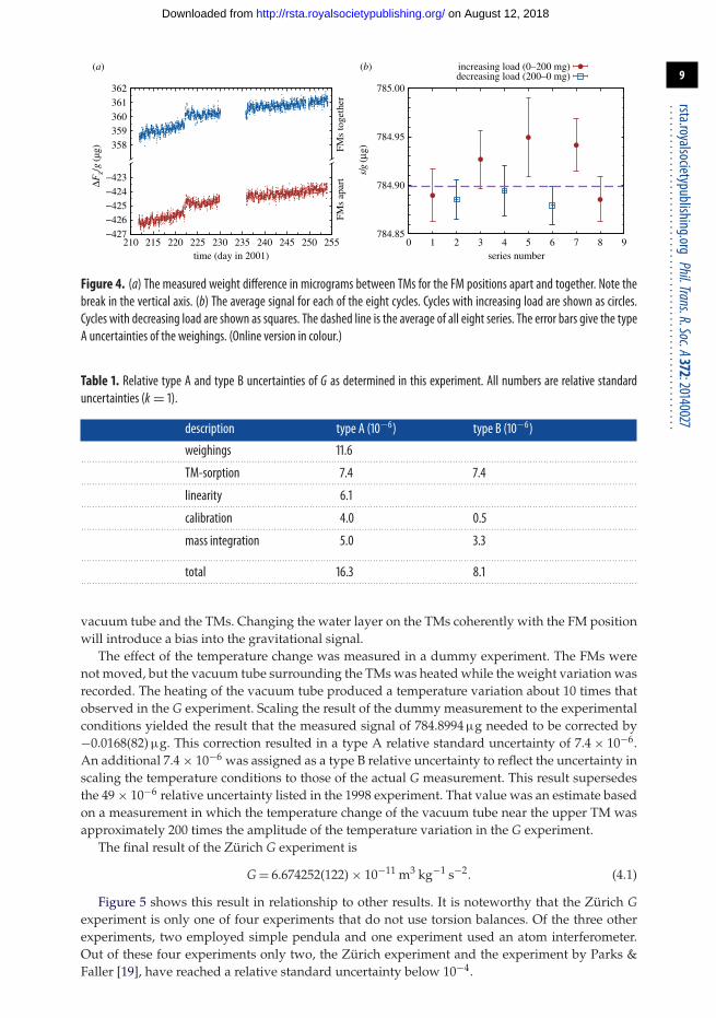
4. Measurements and resultThe data used in the final G result were measured during 44 days in the late summer of 2001.Figure 4 shows the measured weight difference between the two TMs for the two FM positions.One can see a balance drift and other disturbances, e.g. a jump on day 222 most likely caused byloss or gain of a dust particle. However, all these effects are common mode, i.e. they cancel in thesecond difference.

The data shown in figure 4 consist of eight nearly complete cycles. A cycle is a measurement ofG with all 256 possible load values that can be achieved with the two sets of AMs, two TMs andthe apart and together positions of the FMs. There are 2304 individual weighings in one completecycle. The load was applied in either an increasing (from 0 to 200 mg) or a decreasing (from 200to 0 mg) fashion. Of the eight cycles, five were taken in increasing order. The measured value ofthe gravitational signal is shown in figure 4b.

The uncertainty budget is shown in table 1. The largest contribution is from the statisticalscatter of the weighing data contributing a relative uncertainty of 11.6 × 10−6. The next largesteffect is water sorption on the TMs. Combining type A and type B uncertainties in this categoryyields a relative uncertainty of 10.5 × 10−6. This effect is due to a different air flow around thevacuum tube for the FMs in position A and T. Hence, the temperature of the vacuum tube changesslightly: about 0.04 K and 0.01 K for the regions around the upper and lower TMs, respectively.This temperature change will result in a redistribution of the adsorbed water layers on the

on August 12, 2018http://rsta.royalsocietypublishing.org/Downloaded from

9

rsta.royalsocietypublishing.orgPhil.Trans.R.Soc.A372:20140027

.........................................................

358359360361362

(a) (b)

FMs

toge

ther

DFz/

g(µ

g)

−427−426−425−424−423

210 215 220 225 230 235 240 245 250 255

FMs

apar

t

time (day in 2001)

784.85

784.90

784.95

785.00

0 1 2 3 4 5 6 7 8 9

s/g

(mg)

series number

increasing load (0–200 mg)decreasing load (200–0 mg)

Figure 4. (a) The measured weight difference in micrograms between TMs for the FM positions apart and together. Note thebreak in the vertical axis. (b) The average signal for each of the eight cycles. Cycles with increasing load are shown as circles.Cycles with decreasing load are shown as squares. The dashed line is the average of all eight series. The error bars give the typeA uncertainties of the weighings. (Online version in colour.)

Table 1. Relative type A and type B uncertainties of G as determined in this experiment. All numbers are relative standarduncertainties (k = 1).

description type A (10−6) type B (10−6)

weighings 11.6. . . . . . . . . . . . . . . . . . . . . . . . . . . . . . . . . . . . . . . . . . . . . . . . . . . . . . . . . . . . . . . . . . . . . . . . . . . . . . . . . . . . . . . . . . . . . . . . . . . . . . . . . . . . . . . . . . . . . . . . . . . . . . . . . . . . . . . . . . . . . . . . . . . . . . . . . . . . . . . . . . . . . . . . . . . . . . . . . . . . . . . . . . . . . . . . . . . . . . . . . .

TM-sorption 7.4 7.4. . . . . . . . . . . . . . . . . . . . . . . . . . . . . . . . . . . . . . . . . . . . . . . . . . . . . . . . . . . . . . . . . . . . . . . . . . . . . . . . . . . . . . . . . . . . . . . . . . . . . . . . . . . . . . . . . . . . . . . . . . . . . . . . . . . . . . . . . . . . . . . . . . . . . . . . . . . . . . . . . . . . . . . . . . . . . . . . . . . . . . . . . . . . . . . . . . . . . . . . . .

linearity 6.1. . . . . . . . . . . . . . . . . . . . . . . . . . . . . . . . . . . . . . . . . . . . . . . . . . . . . . . . . . . . . . . . . . . . . . . . . . . . . . . . . . . . . . . . . . . . . . . . . . . . . . . . . . . . . . . . . . . . . . . . . . . . . . . . . . . . . . . . . . . . . . . . . . . . . . . . . . . . . . . . . . . . . . . . . . . . . . . . . . . . . . . . . . . . . . . . . . . . . . . . . .

calibration 4.0 0.5. . . . . . . . . . . . . . . . . . . . . . . . . . . . . . . . . . . . . . . . . . . . . . . . . . . . . . . . . . . . . . . . . . . . . . . . . . . . . . . . . . . . . . . . . . . . . . . . . . . . . . . . . . . . . . . . . . . . . . . . . . . . . . . . . . . . . . . . . . . . . . . . . . . . . . . . . . . . . . . . . . . . . . . . . . . . . . . . . . . . . . . . . . . . . . . . . . . . . . . . . .

mass integration 5.0 3.3. . . . . . . . . . . . . . . . . . . . . . . . . . . . . . . . . . . . . . . . . . . . . . . . . . . . . . . . . . . . . . . . . . . . . . . . . . . . . . . . . . . . . . . . . . . . . . . . . . . . . . . . . . . . . . . . . . . . . . . . . . . . . . . . . . . . . . . . . . . . . . . . . . . . . . . . . . . . . . . . . . . . . . . . . . . . . . . . . . . . . . . . . . . . . . . . . . . . . . . . . .

total 16.3 8.1. . . . . . . . . . . . . . . . . . . . . . . . . . . . . . . . . . . . . . . . . . . . . . . . . . . . . . . . . . . . . . . . . . . . . . . . . . . . . . . . . . . . . . . . . . . . . . . . . . . . . . . . . . . . . . . . . . . . . . . . . . . . . . . . . . . . . . . . . . . . . . . . . . . . . . . . . . . . . . . . . . . . . . . . . . . . . . . . . . . . . . . . . . . . . . . . . . . . . . . . . .

vacuum tube and the TMs. Changing the water layer on the TMs coherently with the FM positionwill introduce a bias into the gravitational signal.

The effect of the temperature change was measured in a dummy experiment. The FMs werenot moved, but the vacuum tube surrounding the TMs was heated while the weight variation wasrecorded. The heating of the vacuum tube produced a temperature variation about 10 times thatobserved in the G experiment. Scaling the result of the dummy measurement to the experimentalconditions yielded the result that the measured signal of 784.8994 µg needed to be corrected by−0.0168(82) µg. This correction resulted in a type A relative standard uncertainty of 7.4 × 10−6.An additional 7.4 × 10−6 was assigned as a type B relative uncertainty to reflect the uncertainty inscaling the temperature conditions to those of the actual G measurement. This result supersedesthe 49 × 10−6 relative uncertainty listed in the 1998 experiment. That value was an estimate basedon a measurement in which the temperature change of the vacuum tube near the upper TM wasapproximately 200 times the amplitude of the temperature variation in the G experiment.

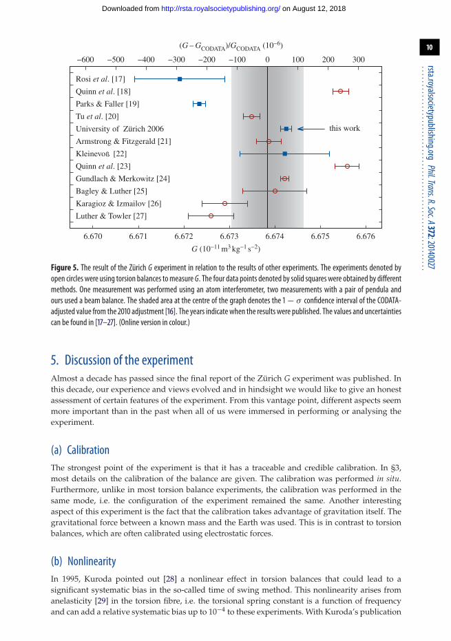
The final result of the Zürich G experiment is

G = 6.674252(122) × 10−11 m3 kg−1 s−2. (4.1)

Figure 5 shows this result in relationship to other results. It is noteworthy that the Zürich Gexperiment is only one of four experiments that do not use torsion balances. Of the three otherexperiments, two employed simple pendula and one experiment used an atom interferometer.Out of these four experiments only two, the Zürich experiment and the experiment by Parks &Faller [19], have reached a relative standard uncertainty below 10−4.

on August 12, 2018http://rsta.royalsocietypublishing.org/Downloaded from

10

rsta.royalsocietypublishing.orgPhil.Trans.R.Soc.A372:20140027

.........................................................

this work

−600 −500 −400 −300 −200 −100 0 100 200 300

(G – GCODATA)/GCODATA (10−6)

6.670 6.671 6.672 6.673 6.674 6.675 6.676

G (10−11 m3 kg−1 s−2)

Karagioz & Izmailov [26]

Luther & Towler [27]

Bagley & Luther [25]

Gundlach & Merkowitz [24]

Quinn et al. [23]

Armstrong & Fitzgerald [21]

University of Zürich 2006

Tu et al. [20]

Parks & Faller [19]

Quinn et al. [18]

Rosi et al. [17]

Kleinevo [22]

Figure 5. The result of the Zürich G experiment in relation to the results of other experiments. The experiments denoted byopen circles were using torsion balances tomeasure G. The four data points denoted by solid squares were obtained by differentmethods. One measurement was performed using an atom interferometer, two measurements with a pair of pendula andours used a beam balance. The shaded area at the centre of the graph denotes the 1 − σ confidence interval of the CODATA-adjusted value from the 2010 adjustment [16]. The years indicate when the results were published. The values and uncertaintiescan be found in [17–27]. (Online version in colour.)

5. Discussion of the experimentAlmost a decade has passed since the final report of the Zürich G experiment was published. Inthis decade, our experience and views evolved and in hindsight we would like to give an honestassessment of certain features of the experiment. From this vantage point, different aspects seemmore important than in the past when all of us were immersed in performing or analysing theexperiment.

(a) CalibrationThe strongest point of the experiment is that it has a traceable and credible calibration. In §3,most details on the calibration of the balance are given. The calibration was performed in situ.Furthermore, unlike in most torsion balance experiments, the calibration was performed in thesame mode, i.e. the configuration of the experiment remained the same. Another interestingaspect of this experiment is the fact that the calibration takes advantage of gravitation itself. Thegravitational force between a known mass and the Earth was used. This is in contrast to torsionbalances, which are often calibrated using electrostatic forces.

(b) NonlinearityIn 1995, Kuroda pointed out [28] a nonlinear effect in torsion balances that could lead to asignificant systematic bias in the so-called time of swing method. This nonlinearity arises fromanelasticity [29] in the torsion fibre, i.e. the torsional spring constant is a function of frequencyand can add a relative systematic bias up to 10−4 to these experiments. With Kuroda’s publication

on August 12, 2018http://rsta.royalsocietypublishing.org/Downloaded from

11

rsta.royalsocietypublishing.orgPhil.Trans.R.Soc.A372:20140027

.........................................................

nonlinearity became a prime concern in experiments determining the gravitational constant.Unfortunately, most of the effort is spent on anelasticity of torsion fibre. This is certainly animportant, but not the only, source of nonlinearity.

Nonlinearity can occur in any instrument. Linearity of an experimental apparatus shouldnever be taken for granted. After obtaining a first result with the Zürich G experiment in 1998,the experimenters were unable to ascertain the linearity of the mass comparator and a generousrelative uncertainty of 200 × 10−6 was assigned to it.

Subsequently, the nonlinearity was investigated; see §3. The result showed a remarkably smallcontribution due to nonlinearity of the mass comparator. The relative standard uncertainty due tononlinearity was only 6.1 × 10−6. Although the nonlinearity of the balance was not a large effectin our experiment, it was a good investment of time and effort to know this for certain.

(c) Large gravitational signalThe gravitational signal in this experiment is large, i.e. the second difference corresponds to7.7 µN. For comparison with the torsion–pendulum measurements of [18,24], the correspondinggravitational forces are approximately 0.3 µN and 1.5 × 10−4 µN, respectively. Thus, the forcesproducing the signals in these two measurements are a factor of 25 and 50 000 times smaller thanthat of the Zürich experiment.

Having a large gravitational force acting on the TMs reduces the relative size of parasitic forcesthat arise due to surface potentials, gas pressure forces and other disturbances.

(d) Symmetry and geometryThe experiment has beautiful symmetry. This symmetry is one of the key points enabling theprecision that the experiment finally achieved. The centre of mass of the FMs remains at one point.The FMs are supported by three spindles that have a right-hand thread on the upper part and aleft-hand thread on the lower part. Thus, as one FM moves down, it pushes the other field massup. Other than friction, no mechanical work is performed in moving from position A to positionT. Therefore, a relatively small motor was used to move the FMs. As an example, to overcome thepotential energy of raising one FM in the 5 min that it takes to change from position A to T, 180 Wof power would be required.

Besides motor power versus temperature, the symmetric set-up has another advantage: thesystem does not tilt. The support structure that connects the FM assembly to the ground of theexperiment has to take up the same force and torques independent of the FM position.

The gravitational field on-axis of a hollow cylinder centred at the origin with inner diameterR1, outer diameter R2, height 2B and density ρ is given by

V(1) = gz(0, 0, z) = 2πρG(r+2 − r−

2 + r−1 − r+

1 ) with r±1,2 =

√R2

1,2 + (z ± B)2. (5.1)

The potential off-axis can be found easily by using a Taylor expansion of gz(r, 0, z) for small r.Assuming azimuthal symmetry will yield non-zero coefficients only for even exponents of r.

From the above equation, it can be seen that the vertical component of the gravitational fieldnear the end of the hollow cylinder (r = 0, z ≈ B) has the shape of a saddle surface, i.e. it hasa maximum along the axial direction and a minimum in the radial direction. As the TMs arelocated at the saddle points, the accuracy required to measure their position can be achieved withonly moderate effort. The vertical and horizontal positions of both TMs relative to the FMs wereobtained with an accuracy of about 0.1 mm in the horizontal direction and 0.035 mm in the verticaldirection. The measurements were performed using surveyors’ tools: a theodolite for horizontalpositions and a levelling instrument for vertical positions.

While we only had to measure the positions of the TMs with moderate precision, the massdistribution of the inner parts of the vessels had to be known with high accuracy. Hence, theseparts were machined with tight tolerances and measured on a coordinate measuring machine

on August 12, 2018http://rsta.royalsocietypublishing.org/Downloaded from

12

rsta.royalsocietypublishing.orgPhil.Trans.R.Soc.A372:20140027

.........................................................

(CMM) with small uncertainties. For example, the central bores of the hollow cylinders werehoned to achieve the required standard uncertainty of 1 µm on the inner diameter.

The uncertainties of the dimensions of the TMs, of the dimensions of the FMs, and of theirrelative positions sum up to relative standard uncertainty in the final result of 4.95 × 10−6. Thisnumber includes the mercury density and mass via the constraint fit (see §5f ). This uncertaintyis part of the 5.0 × 10−6 listed under type A and mass integration. The remainder is due touncertainties in the mass measurements of the steel components of the vessels.

(e) Vertical systemFrom an objective viewpoint, measuring parallel to the direction of local gravity seems ill-conceived. One has to measure the minuscule gravitational signal (785 µg) on top of a largebackground (1 kg). The ratio of background to signal is 1.3 × 106. As the sensitivity of theexperiment is 10−5 times the signal, the ratio of sensitivity to background is 1.3 × 1011. This isa really large ratio for a mechanical experiment. From these numbers, it is obvious that a verticalexperiment needs a much higher ratio of sensitivity to background than a horizontal experiment.This is one of the reasons why several attempts in this geometry achieved uncertainties of 10−3

or larger [30,31].Two factors mediate this disadvantage in the Zürich G experiment: first, the mass comparator

is constructed such that a large fraction of the applied force is balanced by a built-in counter massand only a small part of the force (4 × 10−3) has to be produced by an electromagnetic actuator.Second, state-of-the-art mass comparators have a fantastic sensitivity. The commercial version ofthe AT1006 has a relative resolution of 10−10.

(f) Liquid field massesThe experiment employs two liquid FMs, i.e. 90% of the gravitational signal is contributed byliquid mercury and only about 10% by both vessels. A liquid minimizes density inhomogeneitiesat the expense of requiring a vessel that can hold the liquid. Indeed, the uncertainty in thedensity inhomogeneity of the mercury was only a small contribution to the total uncertaintyof the experiment. The absolute value of the density of mercury was determined at thePhysikalisch Technischen Bundesanstalt in Germany with a relative uncertainty of 3 × 10−6. Fromthis measurement, the known temperature, thermal expansion and isothermal compressibilitya density profile of the mercury in the vessels could be calculated. Modelling the vessels forthe mass integration was cumbersome. Both vessels were broken up into 1200 objects, withpositive and negative density. Simple rotational shapes with rectangular, triangular or circularcross sections were used. Negative density was employed to take away from previously modelledspace. This was used, for example, for bolt holes and O-ring grooves.

While mercury had a known density gradient due to its compressibility, density variationsin the stainless steel used to manufacture the vessels were unknown. This was especiallyproblematic for the parts that were close to the TMs. A density variation in these parts couldhave affected the result of the experiment. In order to investigate this, the inner pieces of thevessels were cut into rings after the experiment ended (three rings near the top and three near thebottom of each central tube). The density of each ring was determined by weighing each ring andmeasuring its dimensions with a CMM. With this method, a standard uncertainty of 0.001 g cm−3

was achieved. The average density of the rings was 7.908 g cm−3. The largest variation of thedensity was only 0.1%, which had only a negligible effect on the mass-integration constant.

Another interesting issue arose from deformation after loading the vessels with mercury.The four main parts used to assemble each vessel were carefully measured on a CMM. However,the load and hydrostatic pressure deformed the vessels. To take this into account, the shapesof the top and bottom of the full vessels were measured with a laser tracker (LT). From theCMM and LT measurements combined with equations describing the bending of thin cylindricalshells [32], the final shape of the vessels could be determined.

on August 12, 2018http://rsta.royalsocietypublishing.org/Downloaded from

13

rsta.royalsocietypublishing.orgPhil.Trans.R.Soc.A372:20140027

.........................................................

The liquid FMs had one, originally not anticipated, advantage: as the geometrical dimensionsof one mercury volume (inner radius r, outer radius R and height h), the mass of the mercurym and the density of the mercury were known, one could set up a system of equations with aconstraint on the volume, mass and density. By using a least-squares adjustment of χ2 given by

χ2 =(

r − r0

σr

)2+

(R − R0

σR

)2+

(h − h0

σh

)2+

(m − m0

σm

)2+

(ρ − ρ0

σρ

)2(5.2)

the uncertainties on the four parameters can be substantially improved. Here, the quantities witha subscript denote measured values or their standard uncertainties and those without a subscriptrefer to the adjusted values. This procedure introduces correlations between the adjustedparameters, but this is a small price to pay compared with the improvement in uncertainty: byusing the constraint, the uncertainty component caused by the geometric uncertainties in the massintegration could be reduced by a factor of 7.

6. SummaryFrom 1994 to 2006, seven scientists worked on the Zürich G experiment with various degrees ofoverlap. Their combined work resulted in the value G = 6.674252(122) × 10−11 m3 kg−1 s−2. Therelative standard uncertainty of the measurement is 18 × 10−6. In recent history, this experimentis only one of two that have not used a torsion balance and have produced a result with a relativeuncertainty smaller than 100 × 10−6.

Torsion balances are very sensitive instruments and are well adapted to the measurementof small forces such as gravitational forces. However, calibrating a torsion balance is difficultand error-prone [33]. Furthermore, nonlinearities can be a significant effect in measurementsusing torsion balances [28]. Although the calibration of a beam balance is simple and robust,the gravitational signal has to be measured in the presence of a very large background due to theweight of the TM. However, as we have demonstrated, it is possible to obtain a relative statisticalaccuracy of several parts in 106 with this method.

Considering the differences and difficulties of the various approaches, only more data willfinally help to resolve the debate concerning the true value of G. We hope to see many differentexperimental approaches in the future and we encourage the researchers to invest in a credibleand traceable calibration scheme.

References1. Fischbach E, Sudarksy D, Szafer A, Talmadge C, Aronson SH. 1986 Reanalysis of the Eötvös

experiment. Phys. Rev. Lett. 56, 3–6. (doi:10.1103/PhysRevLett.56.3)2. von Eötvös R, Pekár D, Fekete E. 1922 Beiträge zum Gesetze der Proportionalität von Trägheit

und Gravität. Ann. Phys. 373, 11–66. (doi:10.1002/andp.19223730903)3. Stubbs CW, Adelberger EG, Raab FJ, Gundlach JH, Heckel BR, McMurry KD, Swanson HE,

Watanabe R. 1987 Search for an intermediate-range interaction. Phys. Rev. Lett. 58, 1070–1073.(doi:10.1103/PhysRevLett.58.1070)

4. Cornaz A, Hubler B, Kündig W. 1994 Determination of the gravitational constant atan effective interaction distance of 112 m. Phys. Rev. Lett. 72, 1152–1155. (doi:10.1103/PhysRevLett.72.1152)

5. Hubler B, Cornaz A, Kündig W. 1995 Determination of the gravitational constant with alake experiment: new constraints for non-Newtonian gravity. Phys. Rev. D 51, 4005–4016.(doi:10.1103/PhysRevD.51.4005)

6. Schlamminger St, Holzschuh E, Kündig W, Nolting F, Pixley RE, Schurr J, Straumann U.2006 Measurement of Newton’s gravitational constant. Phys. Rev. D 74, 082001. (doi:10.1103/PhysRevD.74.082001)

7. Nolting F. 1998 Determination of the gravitational constant by means of a beam balance:design, construction and first results. PhD thesis, University of Zürich, Zürich, Switzerland.

8. Schlamminger S. 2002 Determination of the gravitational constant using a beam balance. PhDthesis, University of Zürich, Zürich, Switzerland.

on August 12, 2018http://rsta.royalsocietypublishing.org/Downloaded from

14

rsta.royalsocietypublishing.orgPhil.Trans.R.Soc.A372:20140027

.........................................................

9. Schurr J, Nolting F, Kündig W. 1998 Gravitational constant measured by means of a beambalance. Phys. Rev. Lett. 80, 1142–1145. (doi:10.1103/PhysRevLett.80.1142)

10. Schurr J, Nolting F, Kündig W. 1998 Measurement of the gravitational constant G by means ofa beam balance. Phys. Lett. A 248, 295–308. (doi:10.1016/S0375-9601(98)00699-9)

11. Nolting F, Schurr J, Kündig W. 1999 Determination of G by means of a beam balance. IEEETrans. Instrum. Meas. 48, 245–248. (doi:10.1109/19.769574)

12. Nolting F, Schurr J, Schlamminger St, Kündig W. 1999 A value for G from beam-balanceexperiments. Meas. Sci. Technol. 10, 487–491. (doi:10.1088/0957-0233/10/6/312)

13. Nolting F, Schurr J, Schlamminger St, Kündig W. 2000 Determination of the gravitationalconstant G by means of a beam balance. EuroPhys. News 31, 25–27. (doi:10.1051/epn:2000406)

14. Schlamminger St, Holzschuh E, Kündig W. 2002 Determination of the gravitational constantwith a beam balance. Phys. Rev. Lett. 89, 161102. (doi:10.1103/PhysRevLett.89.161102)

15. Schwartz R. 1994 Precision determination of adsorption layers on stainless steel massstandards by mass comparison and ellipsometry: Part 2: sorption phenomena in vacuumMetrologia 31, 129–136. (doi:10.1088/0026-1394/31/2/005)

16. Mohr PJ, Taylor BN, Newell DB. 2012 CODATA recommended values of the fundamentalphysical constants: 2010. Rev. Mod. Phys. 84, 1527–1605. (doi:10.1103/RevModPhys.84.1527)

17. Rosi G, Sorrentino F, Cacciapuoti L, Prevedelli M, Tino GM. 2014 Precision measurementof the Newtonian gravitational constant using cold atoms. Nature 510, 518–521.(doi:10.1038/nature13433)

18. Quinn T, Parks H, Speake C, Davis R. 2013 Improved determination of G using two methods.Phys. Rev. Lett. 111, 101102. (doi:10.1103/PhysRevLett.111.101102)

19. Parks HV, Faller JE. 2010 Simple pendulum determination of the gravitational constant. Phys.Rev. Lett. 105, 110801. (doi:10.1103/PhysRevLett.105.110801)

20. Tu L-C, Li Q, Wang Q-L, Shao C-G, Yang S-Q, Liu L-X, Liu Q, Luo J. 2010 New determinationof the gravitational constant G with time-of-swing method. Phys. Rev. D 82, 022001.(doi:10.1103/PhysRevD.82.022001)

21. Armstrong TR, Fitzgerald MP. 2003 New measurements of G using the measurementstandards laboratory torsion balance Phys. Rev. Lett. 91, 201101. (doi:10.1103/PhysRevLett.91.201101)

22. Kleinevoß U. 2002 Bestimmung der Newtonschen Gravitationskonstanten G. PhD thesis,University of Wuppertal, Wuppertal, Germany.

23. Quinn TJ, Speake CC, Richman SJ, Davis RS, Picard A. 2001 A new determination of G usingtwo methods. Phys. Rev. Lett. 87, 111101. (doi:10.1103/PhysRevLett.87.111101)

24. Gundlach JH, Merkowitz SM. 2000 Measurement of Newton’s constant using atorsion balance with angular acceleration feedback. Phys. Rev. Lett. 85, 2869–2872.(doi:10.1103/PhysRevLett.85.2869)

25. Bagley CH, Luther GG. 1997 Preliminary results of a determination of the Newtonianconstant of gravitation: a test of the Kuroda hypothesis. Phys. Rev. Lett. 78, 3047–3050.(doi:10.1103/PhysRevLett.78.3047)

26. Karagioz OV, Izmailov VP. 1996 Measurement of the gravitational constant with a torsionbalance. Meas. Tech. 39, 979–987. (doi:10.1007/BF02377461)

27. Luther GG, Towler WR. 1982 Redetermination of the Newtonian gravitational constant G.Phys. Rev. Lett. 48, 121–123. (doi:10.1103/PhysRevLett.48.121)

28. Kuroda K. 1995 Does the time-of-swing method give a correct value of the Newtoniangravitational constant? Phys. Rev. Lett. 75, 2796–2798. (doi:10.1103/PhysRevLett.75.2796)

29. Speake CC, Quinn TJ, Davis RS, Richman SJ. 1999 Experiment and theory in anelasticity. Meas.Sci. Technol. 10, 430–434. (doi:10.1088/0957-0233/10/6/303)

30. Schwarz JP, Robertson DS, Niebauer TM, Faller JE. 1999 A new determination of theNewtonian constant of gravity using the free fall method. Meas. Sci. Technol. 10, 478–486.(doi:10.1088/0957-0233/10/6/311)

31. Lamporesi G, Bertoldi A, Cacciapuoti L, Prevedelli M, Tino GM. 2008 Determination of theNewtonian gravitational constant using atom interferometry. Phys. Rev. Lett. 100, 050801.(doi:10.1103/PhysRevLett.100.050801)

32. Timoshenko SP, Woinowsky-Krieger S. 1987 Theory of plates and shells. New York, NY:McGraw-Hill.

33. Michaelis W, Melcher J, Haars H. 2004 Supplementary investigations to PTB’s evaluation ofG. Metrologia 41, L29–L32. (doi:10.1088/0026-1394/41/6/L01)

on August 12, 2018http://rsta.royalsocietypublishing.org/Downloaded from