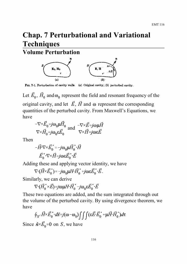
EMT 116

Chap. 7 Perturbational and VariationalTechniquesVolume Perturbation

Let , and represent the field and resonant frequency of the

original cavity, and let , and represent the correspondingquantities of the perturbed cavity. From Maxwell’s Equations, wehave

and

Then

Adding these and applying vector identity, we have.

Similarly, we can derive

These two equations are added, and the sum integrated through outthe volume of the perturbed cavity. By using divergence theorem, wehave

Since on , we have

116

EMT 117

and.

Therefore,

For small perturbation, approximate the cavity fields by , , then

.

We have

where and are time-average electric and magneticenergies originally contained in and is the total energy storedin the original cavity.

It is evident from the preceding equations that an inwardperturbation will raise the resonant frequency if it is made at apoint of large , and will lower the resonant frequency if it ismade at a point of large . It is also evident that the greatestchanges in resonant frequency will occur when the perturbationis at a position of maximum and zero , or vice versa.

117

EMT 118

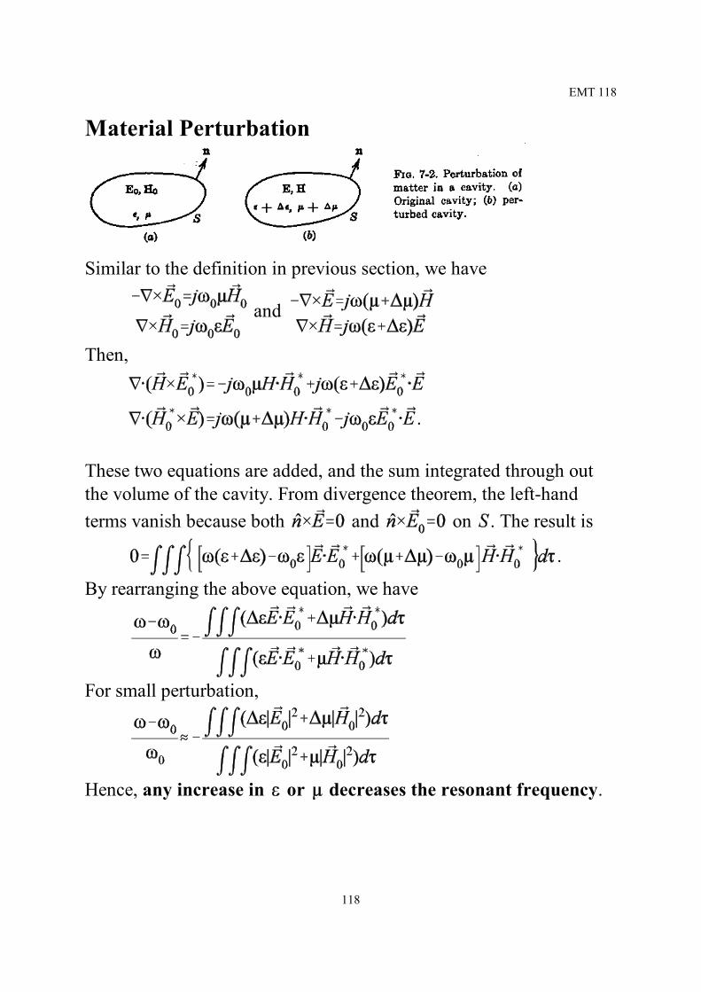
Material Perturbation

Similar to the definition in previous section, we have

and

Then,

.

These two equations are added, and the sum integrated through outthe volume of the cavity. From divergence theorem, the left-handterms vanish because both and on . The result is

.

By rearranging the above equation, we have

For small perturbation,

Hence, any increase in or decreases the resonant frequency.

118

EMT 119

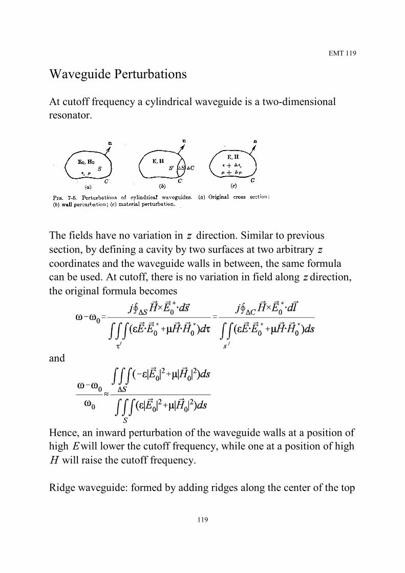
Waveguide Perturbations

At cutoff frequency a cylindrical waveguide is a two-dimensionalresonator.

The fields have no variation in direction. Similar to previoussection, by defining a cavity by two surfaces at two arbitrary coordinates and the waveguide walls in between, the same formulacan be used. At cutoff, there is no variation in field along direction,the original formula becomes

and

Hence, an inward perturbation of the waveguide walls at a position ofhigh will lower the cutoff frequency, while one at a position of high

will raise the cutoff frequency.

Ridge waveguide: formed by adding ridges along the center of the top

119

EMT 120

and bottom walls of a rectangular waveguide.

120

EMT 121

Such ridges will lower the cutoff frequency of the dominant modeand will raise the cutoff frequency of the next higher mode. Hence, agreater range of single-mode operation can be obtained.

Similarly, for material perturbation

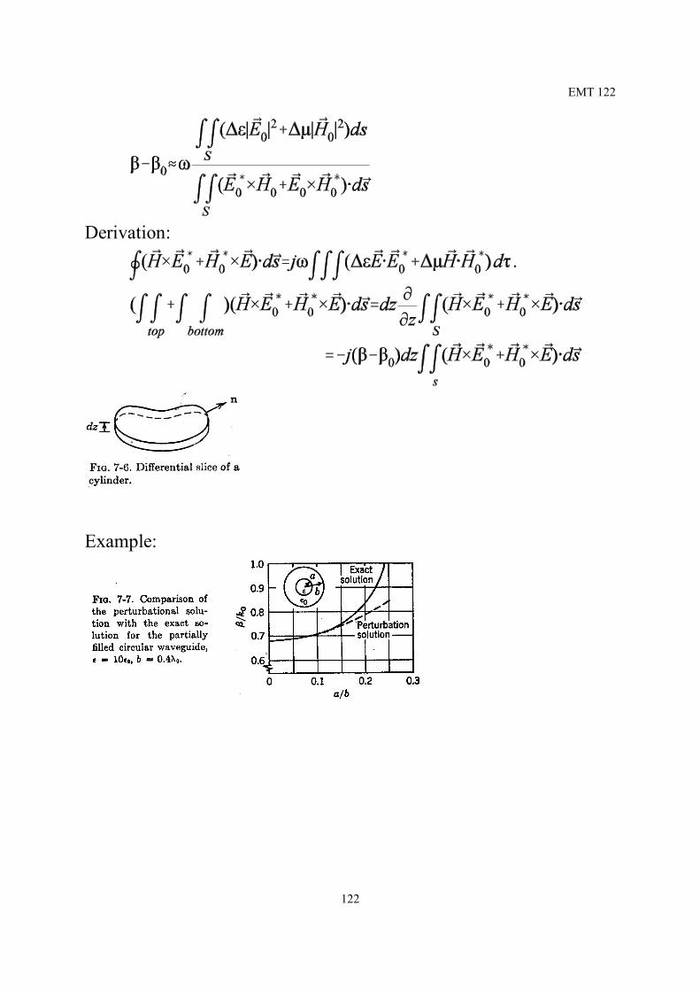
For propagation constant, it can be derived that

121

EMT 122

Derivation:.

Example:

122

EMT 123

Stationary Formulas for Cavities

In a cavity formed by a perfect conductor enclosing a dielectric, thewave equations are

,

By integrating the above equations with and respectively, wehave

(1)

These equations are useful for approximating by assuming fielddistributions in a cavity because of their “stationary” character. Let

where is the true field, is a small arbitrary parameter. Then, wehave

(2)

where we show as a function of for fixed . The Maclaurinexpansion of is

A formula is said to be stationary if the first derivative is zero. Thatis,

To prove the above is true for Eq. (2), let represent the

123

EMT 124

numerator of Eq. (2), then

By vector identity,

.

The last term vanishes, because on . Similarly,

Therefore,

The derivative of the denominator of Eq. (2) is

We then obtain

The above equation vanishes if on , that is on .Hence, Eq. (1) is a stationary formula for the resonant frequency ifthe tangential components of the trial vanish on the cavity wall.

Eq. (1) can be put into a more symmetrical form by applying identity

.

The last term vanishes because on . Eq. (1) becomes

124

EMT 125

Adding a term to the above equation,

(3)

Eq. (3) is the same as previous equation since on . Thedifference is Eq. (3) is stationary even when on .

Similar procedure shows that the formula in Eq. (1) is stationary if

on . Similarly,

(4)

is stationary. however, no boundary conditions on are required.

Example: The dominate mode of a circular cavity is the , theexact resonant frequency and field distributions are

125

EMT 126

Let

Eq. (4) gives . This is 16% higher. Let

which is chosen to satisfy on . This gives ,

only 0.2% in error.

If field formula is used, choose

which satisfy on . This gives , 1.8% in error.

Note: the true first resonant frequency is the absolute minimum.Consider the following equation:

Let , where are the resonant mode fields. Then,

The Ritz Procedure

126

EMT 127

A further advantage of the variational formulation is that one canchoose the best approximation to a stationary quantity obtainablefrom a given class of trial fields. For instance, if we let

,then

The minimum condition becomes

.

This, we can find the best to approximate .

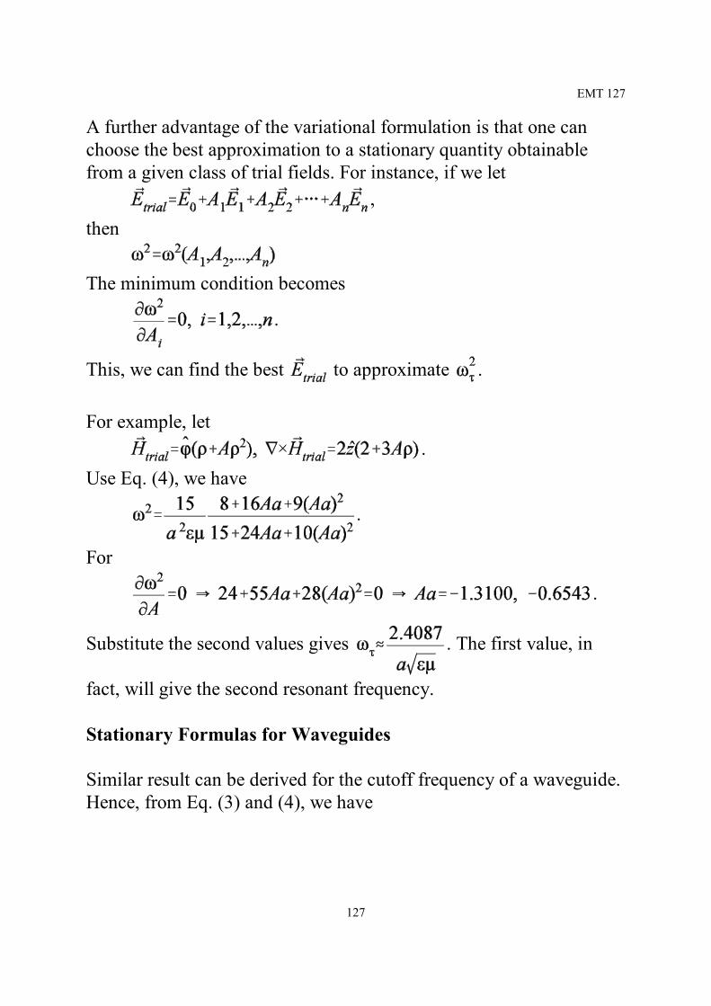
For example, let.

Use Eq. (4), we have

.

For

.

Substitute the second values gives . The first value, in

fact, will give the second resonant frequency.

Stationary Formulas for Waveguides

Similar result can be derived for the cutoff frequency of a waveguide.Hence, from Eq. (3) and (4), we have

127

EMT 128

Example: a partially filled rectangularwaveguide. Let the trial field be the first mode ofan empty waveguide,

.

The result is

For the case and , we have

128

EMT 129

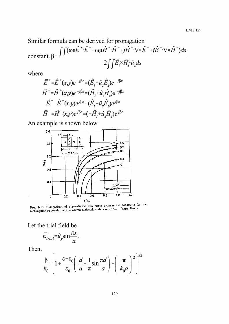
Similar formula can be derived for propagation

constant.

where

An example is shown below

Let the trial field be

.

Then,

129

EMT 130

The Reaction ConceptA general procedure for establishing stationary formulas can beobtained, using the concept of reaction. That is the reaction of field on source is

In general , is stationary if the following condition holds(1)

where and are the correct sources.

Let

then

Using Eq. (1), we have

.Therefore,

.

Example: determining resonant frequencies. The true field atresonance is a source-free field; so the reaction of any field with thetrue source is zero. Then, for self-reactance, we have

(2)

is a stationary formula.

Let be the trial field, then

130

EMT 131

and

on if a boundary is specified. Using the self-reactance formula, wehave

The above equation reduces to the stationary formula of resonancefrequencies in previous section.

Previously, we prove that Eq. (1) is stationary to and , not thefrequency . Let

For a fixed the reaction is a function of both and . SinceEq. (2) must be satisfied always, the first variation of Eq. (2) must bezero, that is

The second term is zero from the proof of Eq. (1), therefore, the firstterm must be zero. Since the coefficient of the first term is not ingeneral zero; so

.Thus, the first variation of vanished. Therefore, it is stationary to

.

Let

131

EMT 132

Then, for .

Therefore,

Example: cylindrical cavity.Let

Then,

132

EMT 133

Stationary Formulas of Impedance

Self Impedance:

Mutual Impedance:

Example:

133

EMT 134

Example: self impedance

Let the trial current be

Enforcing the value of and that satisfy the stationary condition,we have

Solving for and , we have

Therefore,

Rearranging, we have

Since on the antenna surface except at the feed, we have

for any where is the input voltage and is the current at theinput. Therefore,

Assume

134

EMT 135

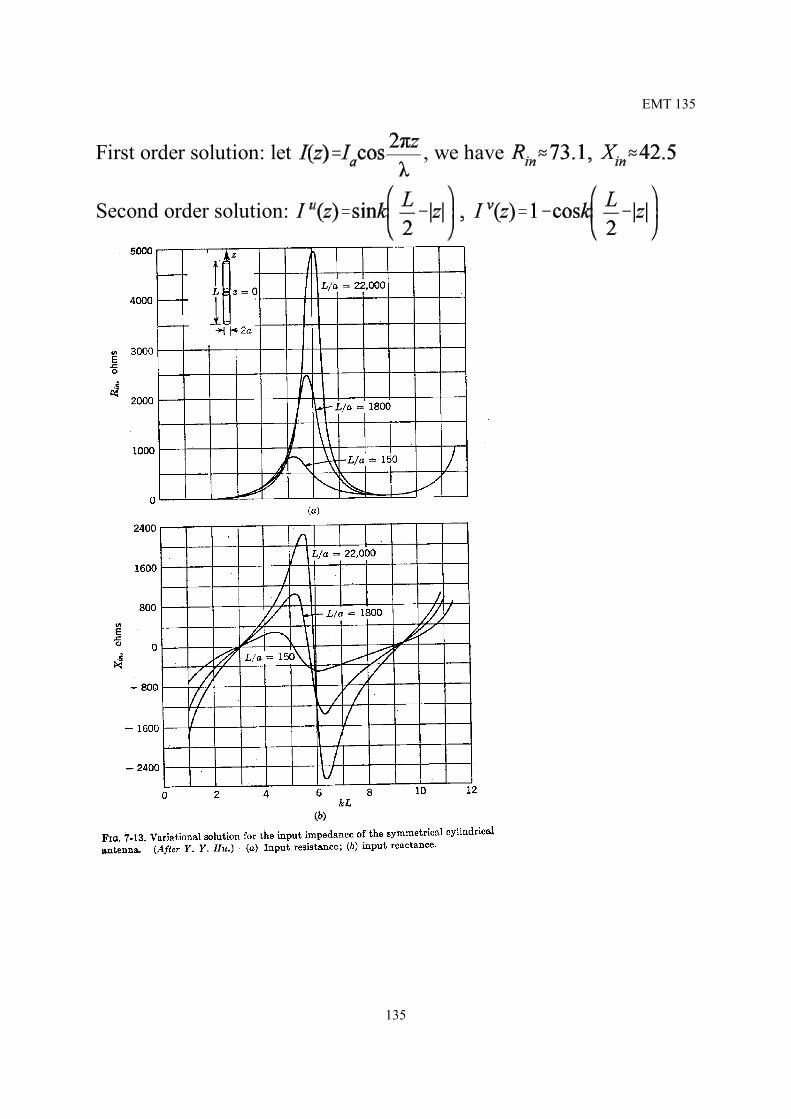
First order solution: let , we have

Second order solution:

135

EMT 136

Stationary Formulas for Scattering

Scattering by a PECAssume , then the following is a stationary formula foreffective area.

Example:

136

EMT 137

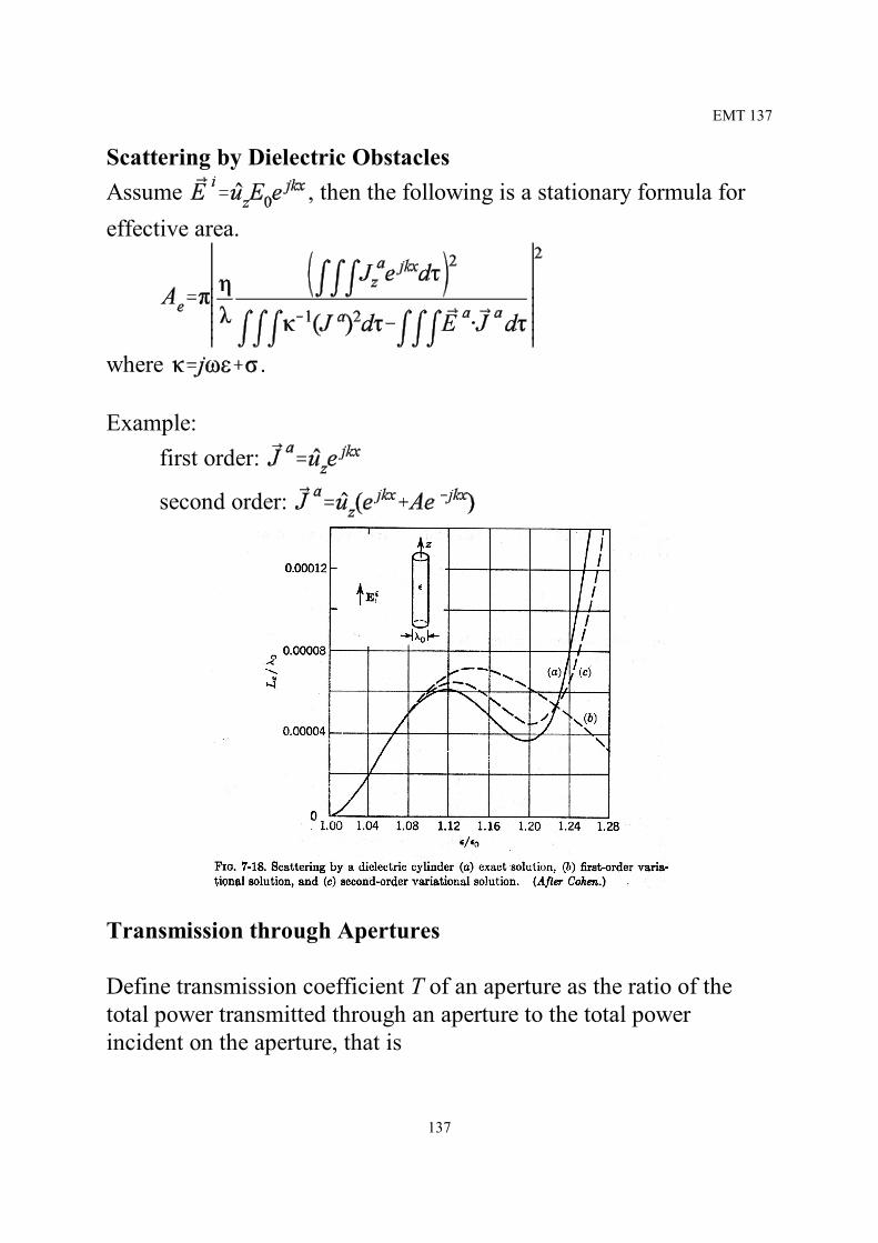
Scattering by Dielectric ObstaclesAssume , then the following is a stationary formula foreffective area.

where .

Example: first order:

second order:

Transmission through Apertures

Define transmission coefficient T of an aperture as the ratio of thetotal power transmitted through an aperture to the total powerincident on the aperture, that is

137

EMT 138

.

Then, the following is a stationary formula for T.

If and is the area of the aperture.

Example: . Let .

138

EMT 139

Chap. 8 Microwave Networks

Introduce mode functions , , mode voltages andmode currents according toTM:

TE:

We can choose forTM:

TE:

Also all modes are normalized according to

Then, the characteristic impedance is

139

EMT 140

These is also the wave impedance. Also and will satisfytransmission-line equations

The power transmitted is

Since

Then for

TE: TM:

140

EMT 141

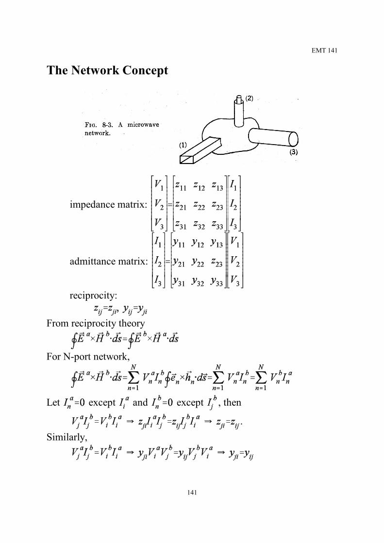
The Network Concept

impedance matrix:

admittance matrix:

reciprocity:

From reciprocity theory

For N-port network,

Let except and except , then

.Similarly,

141

EMT 142

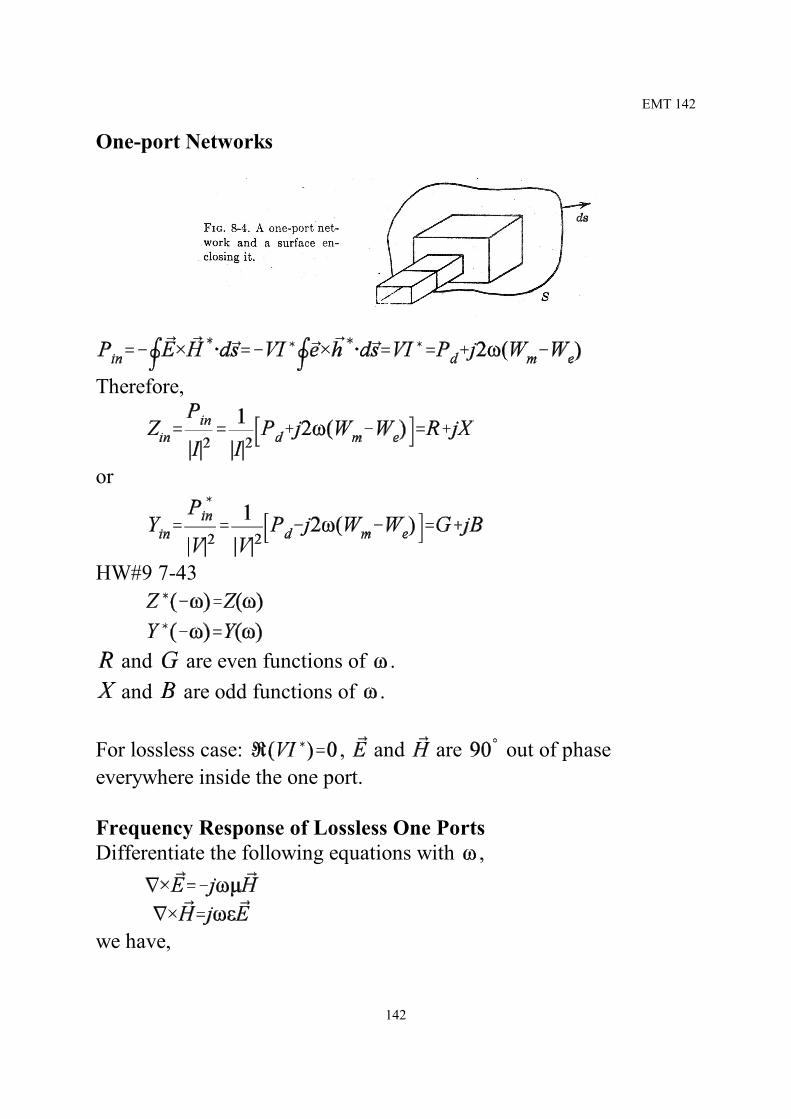
One-port Networks

Therefore,

or

HW#9 7-43

and are even functions of . and are odd functions of .

For lossless case: , and are out of phaseeverywhere inside the one port.

Frequency Response of Lossless One PortsDifferentiate the following equations with ,

we have,

142

EMT 143

Multiply the first equations with and the conjugate of previousequation, and subtract, we have

Similarly,

Subtracting the above two equations, we have

.

By divergence theorem,

.

Apply the above equation to a one-port device, then

Since

,

then,

143

EMT 144

Hence,

This means the slope of and are always positive.Also

Therefore,

Also, expand or at resonant frequency , then

.

Since , has simple zero at and has a simple

pole at . Vice versa.

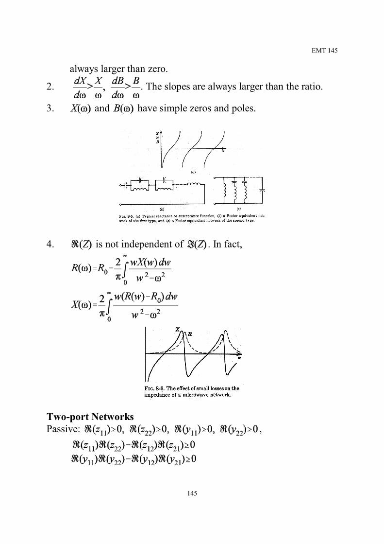
1. . The slope of functions and are

144

EMT 145

always larger than zero.

2. . The slopes are always larger than the ratio.

3. and have simple zeros and poles.

4. is not independent of . In fact,

Two-port NetworksPassive: ,

145

EMT 146

Transmission matrix

T-matrix to S-matrix conversition.

S-matrix to T-matrix conversion

146

EMT 147

Cascading of T-matrix

Modal Expansions in Cavities

Sourceless,

: mode patterns, form a complete set.: mode frequency.

Boundary conditions: (PEC boundaries).

Normalization: which imply

.

Suppose a source exist at frequency , then

Therefore,.

Expand by , then

147

EMT 148

Substitute to previous equation,

Integrate with , then

and,

.

For magnetic source , by duality, we have

Example: a coaxial probe in a cavityAssume:1. The probe current with input current , then2. The equivalent magnetic source on the aperture is negligible.3. Mode fields are chosen to be real.Then,

(pure imaginary if lossless)

where .

148

EMT 149

Low loss, high Q:

then near ,

where is the reactance due to other modes.

Note: the dissipation in modes not near resonance is neglected.

Comparing to the input impedance of an equivalent parallel RLCcircuit,

we have,

Example: rectangular cavity

149

EMT 150

Then,

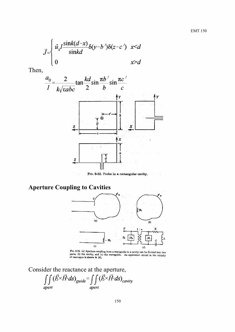
Aperture Coupling to Cavities

Consider the reactance at the aperture,

150

EMT 151

The left hand side lead to

where: mode voltage.: mode characteristic admittance.

: admittance seen by the dominant mode (assume is thedominant mode)Then,

and

For the cavity part,

then,

where.

In the vicinity of a resonant frequency, say , the losses can betaken into account as previous section, therefore

151

EMT 152

In the bracket:1. The first term: the susceptance due to all non-resonant modes.2. The second term: the resonant mode effect.

3.

where is an arbitrary reference voltage, .

Comparing to a series RLC circuit,

we have,

.

Example:Let the field at the aperture be

.

Then, .

Choose . Then, .

The first mode,

Then,

152