Development of Real-time Closed-loop Control Algorithms ... · Development of Real-time Closed-loop...

i

Development of Real-time Closed-loop

Control Algorithms for Grid-scale Battery

Energy Storage Systems

Prepared for the

U.S. Department of Energy

Office of Electricity Delivery and Energy Reliability

Under Cooperative Agreement No. DE-EE0003507

Hawai‘i Energy Sustainability Program

Subtask 3.2: Energy Storage Systems

Submitted by

Hawai‘i Natural Energy Institute

School of Ocean and Earth Science and Technology

University of Hawai‘i

August 2014

ii

Acknowledgement: This material is based upon work supported by the United States

Department of Energy under Cooperative Agreement Number DE-EE0003507.

Disclaimer: This report was prepared as an account of work sponsored by an agency of the

United States Government. Neither the United States Government nor any agency thereof, nor

any of their employees, makes any warranty, express or implied, or assumes any legal liability

or responsibility for the accuracy, completeness, or usefulness of any information, apparatus,

product, or process disclosed, or represents that its use would not infringe privately owned

rights. Reference here in to any specific commercial product, process, or service by tradename,

trademark, manufacturer, or otherwise does not necessarily constitute or imply its

endorsement, recommendation, or favoring by the United States Government or any agency

thereof. The views and opinions of authors expressed herein do not necessarily state or reflect

those of the United States Government or any agency thereof.

iii

Table of Contents

1. Executive Summary ................................................................................................... v

2. Introduction .............................................................................................................. 7

3. ALTI‐ESS Hardware Description ................................................................................. 9

3.1. Overview of HMI and Displays ............................................................................ 15

3.2. Overview of Alarms and Fault Codes ................................................................... 17

3.3. Overview of Control Modes ................................................................................ 18

4. BESS Integration with Utility Grid ............................................................................ 18

4.1. Power One‐Line Diagram .................................................................................... 18

4.2. Signal One‐Line Diagram ..................................................................................... 19

5. Instrumentation ...................................................................................................... 20

6. Data Handling ......................................................................................................... 23

6.1. Communications ................................................................................................. 23

6.2. Data Storage ....................................................................................................... 24

6.3. Data Access ......................................................................................................... 27

7. Algorithm Development Process ............................................................................. 28

7.1. Requirements and Functional Specification Step ................................................. 29

7.2. Architecture and HMI Step .................................................................................. 30

7.3. Simulation Models Step ...................................................................................... 30

7.4. Simulation Results Step ...................................................................................... 30

7.5. Laboratory ATP Step ........................................................................................... 30

7.6. Laboratory ATP Results Step ............................................................................... 31

7.7. Site ATP Step ...................................................................................................... 31

7.8. Site ATP Results Step .......................................................................................... 31

8. Overview of Closed‐loop Control System ................................................................ 31

8.1. Frequency Regulation Algorithm ......................................................................... 32

8.2. Wind Smoothing Algorithm ................................................................................. 32

iv

9. Functional Requirements and Specifications ........................................................... 33

9.1. Frequency Regulation Algorithm Requirements .................................................. 34

9.2. Wind Smoothing Algorithm Requirements .......................................................... 35

10. Architecture of Control Algorithms ....................................................................... 37

10.1. Description of Frequency Regulation Algorithm ................................................ 37

10.2. Description of Wind Smoothing Algorithm ........................................................ 41

11. Simulation and Modeling ...................................................................................... 42

11.1. Frequency Regulation Algorithm ....................................................................... 42

11.2. Wind Smoothing Algorithm ............................................................................... 46

12. Results of Laboratory Simulations ......................................................................... 47

12.1. Frequency Regulation Algorithm Simulation Results ......................................... 48

12.2. Wind Smoothing Algorithm Simulation Results ................................................. 56

13. Conclusion ............................................................................................................ 62

v

1. Executive Summary This report presents the technical work completed under Subtask 3.2, text Item 3.2.2 Control Algorithms conducted under Award Number DE‐EE0003507, Hawaii Energy Sustainability Program (HESP). This effort was funded by the U.S. Department of Energy (DOE), Office of Energy Efficiency and Renewable Energy (EERE), with administration by the National Energy Technology Laboratory (NETL), to the Hawaii Natural Energy Institute (HNEI), School of Ocean and Earth Science and Technology, University of Hawaii at Manoa. The scope of this technical report is to describe the development of the control algorithms and to present simulation results from the two control algorithms. Electricity costs in Hawaii are the highest in the nation due to our small isolated grids and use of oil for over 70% of our power generation. As a result, several islands are experiencing high‐penetrations of wind and photovoltaic systems (PV). On the Hawaii Electric Light Company (HELCO) grid on the Island of Hawaii, wind and distributed PV systems now account for approximately 15% and 3% respectively of total electricity generation. The consequences of utilizing such high‐penetration levels of renewable resources are prominent. Intermittent resources cause grid‐wide imbalances between generation and load, which in‐turn, limit the installation of additional renewable resources. The overall intent of Subtask 3.2 Item 3.2.2) is to support development of control algorithms for evaluation of grid‐connected testing of a Battery Energy Storage System (BESS) to provide grid support. Specifically, control algorithms for both frequency regulation and wind smoothing were developed for assessment of a relatively small, but fast‐acting 1 MW/250 kW‐Hr lithium‐ion (Li‐ion) BESS on the Hawaii Island grid system. During the period between July, 2010 and October, 2012 with separate funding from an Office of Naval Research (ONR) grant the battery was manufactured, tested, and delivered to the Hawi Wind Farm site on the north shore of the Island of Hawaii. The battery was re‐assembled and connected to the HELCO electric grid in November, 2012. Preliminary testing of the battery and balance of system components started in December, 2012. Commissioning, acceptance testing, and analysis of the performance of the BESS with the two control algorithms started in January, 2013. During January to December, 2012 with funding from this DOE grant, the two real‐time control algorithms were developed and installed under technical oversight by, and assistance from HNEI. Using power from the BESS, the frequency regulation algorithm attempts to balance instantaneous grid‐wide mismatches between generation and load within 100 milliseconds (ms), and the wind smoothing algorithm attempts to mitigate strong variations in wind power within 200 milliseconds (ms).

vi

The effect of the frequency regulation algorithm was to typically reduce grid frequency variability by 30% to 40%. The wind smoothing algorithm had the effect of noticeably smoothing the raw wind power and the BESS power. The preliminary results presented in this report support the conclusions drawn from previous simulations. A robust research plan is being developed under separate ONR funding to further the analysis and validation of the BESS, grid, and algorithm performance. Data will be collected and analyzed over the next two years.

7

2. Introduction Under contract to HNEI in 2009 GE Energy Consulting Group ran a Power Systems Analysis Software (PSLF) model of the electric grid on the Island of Hawaii using data from a previous year’s significant frequency down ramp event. Results indicated that a relatively small, 1 megawatt (MW), fast‐acting energy storage system, under the control of a frequency regulation algorithm, could significantly reduce the severity of grid frequency events, essentially reducing grid frequency variability. The results of that simulation are presented in Figure 1. The Blue trace is a plot of the grid frequency data showing the significant wind fluctuation event on May 23, 2007. Note the steep downward ramp event at ~1750 seconds corresponding to a sudden drop in wind power. The Black trace is the result of running the simulation with 1 MW of fast‐acting storage available to the grid for a limited timeframe of 60 seconds. Note the results indicate that a significant reduction in frequency variability is achievable with a small amount of storage for 60 seconds. The Red trace is the result of running the simulation again with 1 MW of storage available continuously. The result is a modest improvement over the performance of the 60 seconds of storage scenario.

Figure 1: Simulation Results from PSLF Model for Significant Wind Event on May 23, 2007

As a result of the promise shown by the simulations, in 2010, HNEI secured funding from ONR to evaluate a grid‐scale BESS which included funding from DOE to support development of real‐time control algorithms. In 2011, HNEI assembled a public‐private partnership to experimentally validate the reduction in grid frequency variability predicted in the simulations. In 2012, the development of a frequency regulation

8

algorithm and a wind smoothing algorithm was initiated. By the end of 2012, the algorithms were installed in the BESS control system. In 1Q 2013 the performance of the algorithms was ready to be assessed at the Hawi Renewable Development LLC (HRD) wind farm (Research Site). The members of the public‐private partnership team are illustrated in Figure 2. A 1 MW/250 kilowatt‐hour (kW‐hr) BESS was manufactured by Altairnano and Parker Hamlin (brand name “ALTI‐ESS”). The HNEI‐led team simulated, designed, and embedded the two control algorithms into the BESS control system. The control system was manufactured by Altairnano and their subcontractors SCADA Solutions and Integrated Dynamics Inc.

Figure 2: Public‐Private Partnership Assembled to Develop and Deploy the Two Control Algorithms

The Island of Hawaii is supplied by the local utility, HELCO. The grid has a daily peak load of approximately 180 MW which occurs between 6pm and 9pm and a minimum load of approximately 80 MW which occurs around 3am. Renewable resources such as wind power, hydro power, distributed photovoltaic systems, and geothermal sources generate 49% of the power on the HELCO grid [IRP 2013]. The Altairnano lithium‐ion ALTI‐ESS was selected as the electrochemistry for this validation project because of its improvement in cycle‐life, recharge time, depth of discharge, and fast‐response power delivery over traditional lithium systems for power‐dependent applications. The ALTI‐ESS was combined with standard utility Balance of Plant equipment which included an Altairnano Battery Management System (BMS) and a real‐time closed‐loop control system (CCS).

9

The scope of this technical report is to describe the development of the two control algorithms and to present the simulation results.

3. ALTI‐ESS Hardware Description The ALTI‐ESS was designed for interconnection to electrical power systems as defined by ANSI C84.1‐2006. It is compliant with the IEEE 1547‐2003 Standard for Interconnecting Distributed Resources with Electric Power Systems when in the discharge mode and the IEEE 519 Standard when in standby or charging modes. The design supports the ALTI‐ESS being stored or operated in the following external ambient site conditions without damaging the system or components when operated properly.

Operating temperature: ‐20 °C to 50 °C

Non‐operating temperature: ‐40 ° to 55 °C

Relative humidity: 0 to 100% condensing

Operating altitude: To 1,000 m above Mean Sea Level without de‐rating

Designed to seismic zone 4 criterion

Designed to Category 3 hurricane (130 mph) criterion

Coastal Environment Corrosion Protection o Premium Power Module Coating system designed for coastal

environments o Stainless Power Control System (PCS) enclosure

The system is comprised of two separate components, a Power Module (PM) and a Power Control System (PCS). The PM is housed in a 53‐ft container and was manufactured by Altairnano ( Figure 3).

10

Figure 3: Power Module (PM) enclosure mounted on trailer prior to shipment to Hawaii

The PM container houses the following subsystems and components:

48‐Line Replaceable Units (LRU), cell‐group components

Battery Management System (BMS) computer

Site Dispatch Controller (SDC computer)

Wiring harnesses

Copper busing

Direct Current (DC) disconnect

Fusing on DC output to the PCS equipment

Knife switches to separate each row of batteries from the battery system

HVAC (heating, ventilation, and air conditioning) temperature set point controllable by BMS

Rack structure and lift mechanism

Ground fault detection system

Fire suppression system The BMS provides the necessary firmware and hardware to control and monitor the 1 MW/250 kW‐hr BESS. The BMS provides an indication of the State‐of‐Charge (SOC), provision to conduct State‐of‐Health (SOH) tests through the Human Machine Interface (HMI), and PM protective features to prevent abuse of the battery. The protective features include:

Prevents over‐charging of the individual cells above 2.8 Volts DC through over voltage detection and PCS shutdown;

Prevents over‐discharging of the individual cells below 1.9 Volts through under voltage detection and PCS shutdown; and

11

Prevents thermal damage of the battery pack through over temperature of the battery pack

The BMS provides climate control, fire detection and suppression, and control and monitoring of the ALTI‐ESS.

The Climate Control system consists of the following components and features:

Two HVAC units

Externally mounted condenser units (designed for coastal environment)

10 kW electric heat in each AC unit

Precision cooling, non‐condensing humidity control

Remote set‐point control capability

Shutdown when fire suppression system discharges The Fire Detection and Suppression system consists of the following components and features:

Compliant with NFPA 12 code

2 Smoke detectors and Heat detectors

Manual pull stations

Master control unit

Key operated arming control box

Central dispersion

Maintenance “by‐pass” valve

Exterior access to carbon dioxide (CO2) bottles for ease of service

Alarms for discharge, trouble and maintenance

HVAC shutdown when discharge occurs The PM has 48 LRUs. Figure 4 shows a single LRU prior to encapsulation and Figure 5 is an interior view of the PM. Each LRU contains four modules and each module contains two cell groups. Each cell group consists of seven Lithium‐ion Titanate 50 ampere – hours (Ahr) cells which represents a cell group capacity of 350 Ahr. The total number of cells in combinations of parallel and series strings is 2,688.

12

Figure 4: Internal view of the Line Replaceable Unit prior to encapsulation

Figure 5: Internal view of the PM. The 1 MW/250 kW‐hr ALTI‐ESS contains 384 “Cell Groups”

or 2688 individual 2.3 Volt (V) 50 Ahr “Cells”

The PCS ( Figure 6), contains a four‐quadrant Inverter, power electronics, and the protection and control system all housed in a “NEMA 4X” Stainless Steel container designed to safely and efficiently interconnect the PCS and PM to the grid. The SDC controls both of these components through two HMI software applications.

13

Figure 6: Power Conversion System Enclosure at Altairnano’s Manufacturing Facility prior to

shipment to Hawaii

The SDC coordinates the charging and discharging of the 1 MW/250 kW‐hr PM to source or sink the desired amount of real or reactive power at the Point of Common Connection (PCC). The SDC has a controller and a PC‐based HMI. The HMI provides an operator console for manual or automatic operation and for maintenance and diagnostic support of the ALTI‐ESS. Figure 7 shows a photograph of the SDC taken during the development stage showing its location in the PM enclosure.

14

Figure 7: Photograph, Courtesy of Altairnano, of the Site Dispatch Controller (SDC)

The SDC includes the following subsystems and components, and capabilities.

Programmable Logic Controller (PLC)

IEEE 1547 Compliance

Read and relay Automated Generation Control (AGC) signal

Provides power commands for the PCS system

Computes the real and reactive power commands for the PCS system

Supports manual‐mode operation

Relay “readiness” signals from the Grid Protection Equipment to the PCS

Commands the PCS Grid Protection breakers to open or close

Programmable to incorporate various modes of operation

System response time from command < 300 millisecond (ms) To ensure the safe and factory specified operation of the ALTI‐ESS the SDC monitors the status and operation of the ALTI‐ESS and provides alarms, automated shutdowns or lockouts when the ALTI‐ESS operational conditions are nearing and/or exceeding preset thresholds of battery voltage and temperature.

15

The PCS includes power electronics and control and communications systems necessary to interface to the PM and the electric grid. When the ALTI‐ESS is connected to the grid at the PCC utilizing Balance of Plant equipment such as breakers, fuses, visible disconnect switches, and step up transformer, the system is renamed and is referred to as the BESS which is an IEEE defined acronym. Control of the BESS is accomplished through the SDC. Compliance with IEEE 1547 is accomplished through robust inverter controls and the use of a Grid Protection Unit (GPU).

3.1. Overview of HMI and Displays

The ALTI‐ESS design includes two HMI screens for local and remote users to interface with the ALTI‐ESS for maintenance, monitoring, and control of the SDC. The PM HMI is located inside the PM and the PCS HMI is located inside the PCS. The PM HMI is a personal computer (PC) that runs the site HMI and PCS HMI software systems. The PM HMI controls the flow of power between the BESS and the electric grid while the PM HMI monitors and controls overall system status, site parameters, and reports fault information for the BESS system. The home screen for the PM HMI is shown in Figure 8. A user identification and password are required to log onto the system. Once logged on, an operator can utilize the buttons on the right hand side of the figure to configure, monitor, control, and trouble shoot the BESS.

Figure 8: Screen Shot of the Home Screen for the Power Module HMI The following BESS information is available thru the PM HMI screen:

16

Battery Pack Summary Information

Cell Group information

Fault Information

HVAC information

Diagnostic information

Configuration and LMU Setup

Current Sensor Calibration

Input voltage, phase‐to‐phase

Input current

Input frequency

State of Charge Indication

Output voltage, phase‐to‐phase and phase‐to‐neutral

Output current

Output frequency

Output kilovolt‐ampere reactive power (KVAr)

Elapsed time meter to indicate hours of operation

Phase‐to‐phase voltage, and phase‐to‐neutral voltage

Output kW, kVAr and power factor

Output kW‐hr DC bus voltage

The Battery Pack Summary Information screen is shown in Figure 9. The screen displays information about the PM such as PM status, faults, operating modes, and summaries of Battery Pack information such as battery SOC, voltage, temperature, active conditions, and faults.

17

Figure 9: Screen Shot of Battery Pack HMI Screen (Part of PM HMI)

3.2. Overview of Alarms and Fault Codes

The BESS provides local audible alarms, and utilizing internet or RTU connections, remote alarms of the following conditions.

Input AC power source failure

Input protective device open

Output protective device open

Overload

Overload shutdown

DC over voltage

Low battery

Battery discharge

Battery protective device open

Equipment over temperature

Inverter off

Inverter fault

Emergency off

Critical load on static bypass

Inverter output over voltage

Inverter output under voltage

Inverter output over frequency

Inverter output under frequency In addition the BESS can be programmed to page and/or email customer supplied pagers or email accounts of the alarm conditions.

18

3.3. Overview of Control Modes

The BESS design includes a capability to operate the system in one of three modes; Automatic Generation Control (AGC), Manual, or CCS. In AGC operation mode, the BESS receives a power command from a remotely located control system. AGC commands arrive every four seconds, and the system responds to them by calculating power commands that result in delivery of either real or reactive power to the grid or removing real or reactive power from the grid, as requested within four seconds. This mode of operation is used in grid frequency regulation applications, where the power command comes from a Grid Control Authority. In Manual operation, a user at an operator’s workstation can command the BESS to receive power from the grid or deliver power to the grid. The BESS responds to the operators commands, except when power commands are issued that would drive the BESS out of its allowed operating ranges, such as overcharge, undercharge, or over temperature. All of the standard diagnostics and designed‐in protections are active. In CCS operation mode, the SDC will calculate power commands in real‐time based upon external frequency and wind power measurements. This is the control mode that was developed for this project. Subsequent sections of this report will describe the CCS architecture, the measurement instrumentation, the algorithms, and a preliminary assessment of the performance of the CCS.

4. BESS Integration with Utility Grid Applicable standards are the IEEE 1547‐2003 Standard for Interconnecting Distributed Resources with Electric Power Systems when the energy storage system is in the discharge mode and the IEEE 519 Standard when the energy storage system is in standby or charging modes. These standards were utilized to grid‐connect the ALTI‐ESS, Balance of Plant equipment, wind farm, and nearby Waimea substation at the PCC. The team, funded under a separate grant from ONR, developed the signal and power one‐line diagrams presented in sections 4.1 and 4.2 to guide the implementation and support the permitting process with the County. The signal and power one‐line diagrams are presented in section 4.1 and 4.2.

4.1. Power One‐Line Diagram

The Power One‐Line Diagram is shown in Figure 10. The bottom left hand side of the drawing shown in Figure 10 labeled Power Module Enclosure Boundary shows the battery pack and the control unit plus the SDC. Also shown is the Shark 200 meter and corresponding Current Transformer (CT). The Shark 200 meter is connected to a 480 V/480 V 100 kVA isolation transformer through a circuit breaker to the step‐up transformer and the Low Voltage Disconnect Switch (LVDS). The Shark meter is utilized to determine the amount of Aux power, in kW, consumed by the BESS.

19

Figure 10: Power One‐Line Diagram for the BESS at the Research Site

The middle left hand side of the drawing shown in Figure 10 labeled the Power Control System Enclosure Boundary shows the inverter and the connection to the LVDS. The output side of the LVDS is connected to the 1 MVA 480 V/35.4k V step‐up transformer which is connected through a 40 A fuse to the customer lockable group operated 600 A disconnect switch. The output side of the 40 A fuse is the PCC. The upper right hand side of the drawing shown in Figure 10 shows the connection of the wind farm to the PCC through a lockable group operated 600 A disconnect switch. The HELCO substation at Waimea is connected at the PCC to the wind farm and BESS through the 600 A lockable group operated 600 A disconnect switch.

4.2. Signal One‐Line Diagram

The Signal One‐Line‐Diagram is shown in Figure 11. The lower left hand side of the drawing shown in Figure 11 labeled the Power Module Enclosure Boundary shows the media converter, fiber optic, and Ethernet connections to the SDC and BMS subsystems and balance of system components.

20

Figure 11: Signal One‐Line Diagram for the BESS at the Research Site

The upper left hand side of the drawing shown in Figure 11 labeled the Power Control System Enclosure Boundary shows the 1 MW battery pack and inverter and the hard wired connections to the AC breaker and the PCS Master Controller along with the fiber optic interconnections to the grid monitoring and protection subsystems. The BESS utilizes a combination of two meters, the SEL‐735P and SEL‐700GT, to provide over and under frequency protection and over and under voltage protection. The upper right hand side of the drawing shown in Figure 11 labeled HELCO Control Room Boundary shows the RTU and HRD router plus the required communication links between HELCO, the HRD wind farm, and the BESS.

5. Instrumentation The instruments selected for the project are manufactured by Schweitzer Engineering Laboratory and Electro Industries. The SEL 735P Power Quality Meter and the Shark 200 Data Logging Power Meter are shown in Figure 12.

21

Figure 12: Photographs, Courtesy of Schweitzer Engineering Laboratories and Electro Industries, of (Left) a SEL 735P Power Quality Meter and (Right) a Shark 200 Data Logging

Power Meter

The type of measurements and accuracies of each measurement supporting the Frequency Regulation and Wind Smoothing algorithms are shown in Table 1.

Table 1: Required Measurements and Accuracy of each Measurement

At the PCC, the Totalizer meter (SEL‐735P) is utilized to collect frequency, voltage, and current measurements of the grid at a sample rate of 10 Hz for real‐time control of the algorithm and at a sample rate of 5 Hz to store the data in the Cloud Server data base.

22

The power meter in the PM (SEL‐735P) is utilized to sample real and reactive power at a sample rate of 5 Hz. Battery pack temperature is derived from a temperature measurement at a sample rate of 1 minute for each ½ LRU (2‐modules). The location of the instrumentation necessary to acquire the data needed to run the Frequency Regulation algorithm is shown in Figure 13. Each meter is connected to the electric grid through a CT and Potential Transformer (PT).

Figure 13: Locations of Battery, Wind, and Totalizer Meters Providing Input Signals for the

Frequency Regulation Algorithm

The location and type of instrumentation necessary to acquire the data are shown in Figure 14. Each meter is connected to the electric grid through a CT and PT.

23

Figure 14: Locations of Wind and Totalizer Meters Providing Input Signals for the Wind

Smoothing Algorithm

6. Data Handling The SDC is connected to the Internet over encrypted connections for data logging, real‐time monitoring, maintenance and operations support, and to support remote and secure queries of the data stored in the Cloud Server data base.

6.1. Communications

The Communications architecture is illustrated in Figure 15. The green trace is a fiber optic loop to connect the SDC located in the PM to the ALTI‐ESS router and SEL‐735P meter located in the HELCO control room. The HELCO control room is co‐located with the HRD control room. The ALTI‐ESS router is connected to the HRD router (upstream device) for access to the Internet. Both routers are configured to allow outgoing TCP connections over port 7777 (tunneled RDF protocol), outgoing TCP port 80 (HTTP), and UDP port 123 (NTP). The upstream HRD router is configured to prevent unauthorized connections to the ALTI‐ESS router on port 502 from the Internet.

24

Figure 15: Communications Architecture and Internet Access Point

The BESS requires a minimum rate of 33 kbps of the available Internet bandwidth to support the data logging requirements. Firewall settings for the ALTI‐ESS router allow incoming port 502 connections (i.e., Modbus TCP), and have closed all other incoming TCP/IP and UDP/IP ports. The router will allow outgoing TCP/IP connections.

6.2. Data Storage The SDC stores the data listed in Table 2 from the Wind Farm meter (SEL‐735P) over Modbus TCP to the Cloud Server maintained by Altairnano. Measurements of the data shown in the table are available to authorized and authenticated users through a web‐based interface requiring a user ID and password.

25

Table 2: Wind Farm Meter (SEL 735P) Data. Sample Rate: 200 ms. Bandwidth Required (Modbus TCP): 8 kbps. Latency Required: ping delay of 3 ms (typical), and 20 ms (worse case).

Database Entry Description UnitsApp.Wind.Current Wind farm current AApp.Wind.Frequency Grid frequency HzApp.Wind.P_Total Real wind power kWApp.Wind.PhaseA_Current Current (Phase A) AApp.Wind.PhaseAB_Voltage Voltage (Phase A-B) VApp.Wind.PhaseB_Current Current (Phase B) AApp.Wind.PhaseBC_Voltage Voltage (Phase B-C) VApp.Wind.PhaseC_Current Current (Phase C) AApp.Wind.PhaseCA_Voltage Voltage (Phase C-A) VApp.Wind.Q_Total Reactive power kVArApp.Wind.Voltage Wind farm voltage V

The communication medium between the SDC and the Wind Farm meter is a fiber optic cable running from the pole‐mounted Totalizer meter to the PM. The SDC stores the data listed in Table 3. Measurements of real and reactive power plus f, V, and i of the 3‐phase HELCO electric grid are available to authorized and authenticated users through a web‐based interface requiring a user ID and password. Table 3: Totalizer Meter (SEL 735P) Data. Sample Rate: 200 ms. Bandwidth Required (Modbus

TCP): 8 kbps. Latency Required: ping delay of 3 ms (typical), and 20 ms (worse case).

Database Entry Description UnitsApp.Totalizer.Frequency Grid frequency HzApp.Totalizer.P_Total Real power kWApp.Totalizer.Q_Total Reactive power kVARApp.Totalizer.Voltage Voltage V

The communication medium between the SDC and the BESS power meter (housed in the HELCO control room) is an Ethernet cable running to a copper to fiber converter. The SDC stores the data listed in Table 4. Measurement data sets are available to authorized and authenticated users through a web‐based interface requiring a user ID and password.

26

Table 4: BESS Meter (SEL 735P) Data. Sample Rate: 200 ms. Bandwidth Required (Modbus TCP): 8 kbps. Latency Required: ping delay of 3 ms (typical), and 20 ms (worse case).

Database Entry Discription Units

PCC.Frequency Grid frequency HzPCC.KVARH_From_Grid Reactive power absorbed kVAr-hrPCC.KVARH_Net Net reactive power kVAr-hrPCC.KVARH_To_Grid Reactive power delivered kVAr-hrPCC.KWH_From_Grid Real power absorbed kWhPCC.KWH_Net Net real power kWhPCC.KWH_To_Grid Real power delivered kWhPCC.P_Total BESS real power kWPCC.PhaseA_Current Phase A current APCC.PhaseAB_Voltage Phase A-B voltage VPCC.PhaseAN_Voltage Phase A-N voltage VPCC.PhaseB_Current Phase B current APCC.PhaseBC_Voltage Phase B-C voltage VPCC.PhaseBN_Voltage Phase B-N voltage VPCC.PhaseC_Current Phase C current APCC.PhaseCA_Voltage Phase C-A voltage VPCC.PhaseCN_Voltage Phase C-N voltage VPCC.Power_Factor Power factor n/aPCC.Q_Total BESS reactive power kVArPCC.V_Unbalance Unbalance %PCC.Voltage Voltage V

Several PM measurements are acquired by a SEL‐735P meter located in the PCS. These measurements are listed in Table 5.

27

Table 5: PCS Meter (SEL 735P) Data. Sample Rate: 200 ms. Bandwidth Required (Modbus TCP): 8 kbps. Latency Required: ping delay of 3 ms (typical), and 20 ms (worse case).

Database Entry Description UnitsChannel[1].PM.Amp_Hours_Charging Amp Hours Charging AhChannel[1].PM.Amp_Hours_Discharging Amp Hours Dis-charging AhChannel[1].PM.APP_Commanded_Charge_Current_Limit BMS Current Charge Limit AmpsChannel[1].PM.APP_Commanded_Discharge_Current_Limit BMS Current Dis-charge Limit AmpsChannel[1].PM.BMS_P_Charge_Limit_Mgmt BMS Power Limit kWChannel[1].PM.CORE_pack_curr_avg Average Current ampsChannel[1].PM.CORE_pack_power_kw Available Power kWChannel[1].PM.CORE_pack_SOC_pct State of Charge %Channel[1].PM.CORE_pack_volt Pack Voltage voltsChannel[1].PM.CORE_Tmax Maximum Temperature (2-Module) degCChannel[1].PM.CORE_Tmin Minimum Temperature (2-Module) degCChannel[1].PM.CORE_Vmax Maximum Voltage (Cell Group) voltsChannel[1].PM.CORE_Vmin Minimum Voltage (Cell Group) voltsChannel[1].PM.HVAC_Actual_Air_Humidity_Unit1 Humidity Reported by HVAC 1 %Channel[1].PM.HVAC_Actual_Air_Humidity_Unit2 Humidity Reported by HVAC 2 %Channel[1].PM.HVAC_Actual_Air_Temperature_Unit1 Air Temperature Reported by HVAC 1 degCChannel[1].PM.HVAC_Actual_Air_Temperature_Unit2 Air Temperature Reported by HVAC 2 degCChannel[1].PM.HVAC_Temperature_Setpoint_Final_Unit1 Temperature Setpoint for HVAC 1 degCChannel[1].PM.HVAC_Temperature_Setpoint_Final_Unit2 Temperature Setpoint for HVAC 2 degCChannel[1].PM.Lifetime_Amp_Hours_Charging Cumulative Amp Hour Charging AhChannel[1].PM.Lifetime_Amp_Hours_Discharging Cumulative Amp Hours Dis-charging AhModule Temperatures (96 Measurments) Temperatures Deg CCell-group Voltages (384 Measurements) Voltages volts

The SDC sends BESS status information to HELCO and receives status and control information from HELCO utilizing the RTU as listed in Table 6.

Table 6: HELCO RTU Status and Control Signals

Device HELCO RTUItem Requirement Data: HELCO RTU => SDC Remote.Allowed_Op_Mode_Remote (dry contact) Data: SDC => HELCO RTU PCC.P_Total (analog)

PCC.Q_Total (analog) Site.GPU.Grid_State (dry contact) Site.GPU.Summary_Trip (dry contact) Site.Channel[0].AC_Sec_Breaker_State (dry contact) Remote.Alarm (dry contact)

The analog inputs to the RTU were configured with 5 k termination resistors for +/‐1 mA inputs. The status points were internally wetted at 24 VDC. The control outputs to the RTU are KUP‐11 type, Form C rated at 10 A and 24 VDC.

6.3. Data Access Figure 16 shows the data flow from the ALTI‐ESS router on site through the HRD router over encrypted connections to the Cloud Server. Also shown are the data flows from the Cloud Server to authorized and authenticated users.

28

Figure 16: Diagram of the Data Access Process

The lower right hand side of the illustration shows how UH researchers access the data from the Cloud Server through an encrypted connection. The bottom center side of the illustration shows how Altairnano’s engineers accessed the BESS during site acceptance testing and then again after installation and commissioning to support operations and maintenances issues and to provide tech support on an as needed basis.

7. Algorithm Development Process Two real‐time control algorithms were designed, modeled, implemented (coded), tested, and deployed following the Algorithm Development Process illustrated as a flow chart in Figure 17.

The development process included defining the control objectives, then developing a series of design documents for the Frequency Regulation and Wind Smoothing algorithms starting with the Requirements and Functional Specifications document and ending with the results from executing the Site Acceptance Test Plan (ATP).

Requirements and Functional Specification

Architecture and HMI

Simulation and Modeling

Simulation Results

Laboratory ATP

Laboratory ATP Results

Site ATP

Site ATP Results

29

Figure 17: Flow Chart of Algorithm Development Process

Figure 18: Flow Chart of Algorithm Development Process

30

7.1. Requirements and Functional Specification Step

The Requirements and Functional Specifications (RFS) Step in the process developed the control objectives and developed the functional requirements to satisfy the overall control objectives of the project as an input into the design of the Architecture and HMI. The RFS document defined the acceptance criteria for the CCS control operation mode, with the control objective being used to quantify how well the CCS satisfied the control objective. Additionally, any performance limitations of the ALTI‐ESS were identified and restrictions such as execution rate and type of measurement signals were included to execute the algorithm. Completion and acceptance of the RFS is an input into the Architecture and HMI step. Refer to [1] and [2].

7.2. Architecture and HMI Step

The Architecture and HMI Step in the process refined the control architecture, designed the block diagram or flowcharts used to describe each algorithm, identified the system definition parameters, tuning parameters, specified the low‐pass filter parameters, detailed the computational requirements, real‐time performance metrics, and developed the laboratory (bench testing) ATP which included the acceptance criteria and metrics. This step included identifying any modifications to existing screens or development of new user screens for the HMI. Completion and acceptance of the design of the Architecture and HMI is an input into the Simulation Models Step. Refer to [3] and [4].

7.3. Simulation Models Step

The Simulation Models Step in the process developed the simulated laboratory environment concept. A variety of grid models1 were used to study various possible outcomes. This step also defined the architecture of the field‐ready controller hardware and software used in the simulated laboratory environment to test the algorithm as a closed‐loop control system. Completion of the design of the Simulation Models is an input into the Simulation Results Step. Refer to [5] and [6].

7.4. Simulation Results Step

The Simulation Results Step in the process analyzed the results of the simulations and quantified how well the algorithm satisfied the metrics for the control objective. The metrics, developed in the Architecture and HMI step, were used to assess the overall stability and performance of the algorithm and determine if the algorithm was ready to be tested using the laboratory ATP. Completion and acceptance of the Simulation Results is an input into the Laboratory ATP Step. Refer to [5] and [6].

7.5. Laboratory ATP Step The Laboratory ATP Step in the process included developing the ATP, and defining the acceptance criteria to assess the readiness of the control algorithms to be implemented

1 Two key grid models are discussed in this document.

31

(coded) and embedded into the SDC. The ATP included field‐ready controller hardware and software running in a simulated laboratory environment to test the logic and stability of the control algorithms. Completion of the design of the Laboratory ATP is an input into the Laboratory ATP Results Step. Refer to [7] and [8].

7.6. Laboratory ATP Results Step The ATP Results Step in the process verified that the control algorithm implementation satisfied the intent of the control objectives and achieved similar or identical results compared to the simulation. Pass / fail criteria were used to assess the readiness of the control algorithms to be installed in the SDC at the Research Site. Completion and acceptance of the Laboratory ATP Results is an input into the Site ATP Step. Refer to [9] and [10].

7.7. Site ATP Step The Site ATP Step in the process developed the ATP and defined the pass / fail criteria to determine the performance and assess the readiness of the control algorithms to be deployed. The ATP included an assessment of how well the control algorithms met the control objectives and verified that no erroneous power commands were issued by the system. Completion and acceptance of the design of the Site ATP is an input into the Site ATP Results Step.

7.8. Site ATP Results Step The Site ATP Results Step in the process verified that the CCS with either the Frequency Regulation algorithm (responding to changes in frequency of the grid) or the Wind Smoothing algorithm (responding to changes in wind farm output power) met the control objectives given the performance metrics identified in Section 0. Completion and acceptance of the results of the site ATP meant the BESS could be left unattended and with one of the two control algorithms running in the CCS operation mode. Refer to [11] and [12].

8. Overview of Closed‐loop Control System The block diagram of the CCS architecture is shown in Figure 19, it identifies two control algorithms: (1) a frequency regulation algorithm and (2) a wind smoothing algorithm. Key inputs from the SDC and inputs from the HELCO grid, along with power command outputs are included in the block diagram. A description of each algorithm is presented in sections 8.1 and 8.2.

32

Figure 19: Two Real‐time Control Algorithms

8.1. Frequency Regulation Algorithm

A simplified block diagram of the frequency regulation algorithm is shown in Figure 20. The measurement input for the algorithm is grid frequency measured by the BESS SEL‐735P. The estimated SoC is a dynamic input to the algorithm provided by the BMS. Several user‐adjustable input parameters are also inputs to the algorithm.

Figure 20: Simplified Block Diagram for the Frequency Regulation Algorithm.

As shown in the figure, the output power command is a combination of SoC management and an ideal power command based on grid frequency measurements.

8.2. Wind Smoothing Algorithm

A simplified block diagram for the wind smoothing algorithm is shown in Figure 21. The measurement input for the wind smoothing algorithm is wind power measured at the

33

Wind SEL‐735P. The estimated SoC is a dynamic input into the algorithm. Several user‐adjustable input parameters are also inputs to the algorithm.

Figure 21: Simplified Block Diagram for the Wind Smoothing Algorithm

As shown in the figure, the output power command is a combination of SoC management and an ideal power command based on wind power measurements.

9. Functional Requirements and Specifications This section summarizes the functional requirements and specifications for the two algorithms and the corresponding control objectives. The Frequency Regulation and Wind Smoothing algorithms have several common requirements, which include access to the Internet, utility grade power quality meters, measurement sampling rates, measurement resolution, bandwidth, secure data storage, and data access. The control objectives are used to quantify the performance of both algorithms. The control objectives were used during the algorithm development phase to compare alternative control structures, and to assess the performance that can reasonably be expected once the algorithm is deployed. The PCS and PM place limits on the amount of real and reactive power that can be instantaneously delivered by or absorbed by the BESS. The instantaneous real power upper limit is +1.0 MW, and the instantaneous real power lower limit is ‐1.0 MW. Similarly, reactive power (VAr) is limited to +/‐ 1.0 MVAr. The BESS has a limited energy storage capacity. At a 1.0 MW charge / discharge rate, the battery can store up to 250 kW‐hr of energy. As the battery nears full charge state, the allowable charge power limit is reduced, and as the battery nears the fully discharged state, the allowable discharge power limit is reduced. Battery capacity degrades more rapidly when it is operated at high cell temperature for prolonged periods of time. Therefore, there is a tradeoff between operating temperature and cycle life. In order to prevent the battery from running too hot and thereby reducing cycle life, a thermal derating system is included in the BMS. Thermal derating involves making the charge and discharge power limits a function of

temperature. When maximum cell temperature exceeds 52 C, the charge and

34

discharge power limits drop to 500 kW, and once the maximum temperature drops

below 51 C, the power limits return to their normal level of 1.0 MW. The time that is required by the SDC to compute a power command is 100 ms or less. The CCS design must provide acceptable performance (see Section 9) even if the delay is longer than the design limit of 100 ms. The BESS delivers real power that is close to, but not equal to the real power command. The accuracy is assumed to be a multiplier. The actual power delivered is between 90% and 110% of the power command. The realized power command will not exceed ±1.0 MW.

9.1. Frequency Regulation Algorithm Requirements

The requirements and functional specifications document defines the acceptance criteria for the CCS implementation (Section 9), with a control objective used to quantify how well the CCS addressed the frequency regulation problem. The control objective is based on frequency variability. Variability is defined as a root‐mean‐squared (RMS) value of a time series. To evaluate variability at different timescales, the calculation shown in Figure 22 was used.

High Pass Filter• Timescale seconds,• Cutoff = (1/) radians/s

MeasuredGridFrequency

CalculateRMS

Figure 22: Calculation of RMS at various timescales

In this calculation, the time series for grid frequency is fed into a 4th order Butterworth high pass filter with a cutoff frequency of:

1c

Equation 1

In Equation 1, is the timescale limit. The RMS value is computed for the output of the

filter. This calculation can be repeated at different values of to obtain a curve of variability at different timescales. The control objective is shown as a black line in Figure 23.

35

Figure 23: Control Objective (Black Line).

The figure shows that the continental US grid meets the specified control objective, while the two samples from the Island of Hawaii grid do not. The objective of the frequency regulation algorithm is to reduce grid frequency variability (across all of the time scales shown) below the control objective (Black Line).

9.2. Wind Smoothing Algorithm Requirements

The requirements for the wind smoothing CCS include the following:

Minimum data acquisition rate: One sample every 200 ms

Maximum time to calculate power command : 180 ms or less

Maximum rate of missed power commands: One (1) non‐computed response per hour

9.2.1. Energy Management

The CCS manages the PM so that the SOC does not exceed 95% or drop below 5% more than an aggregated value of 10 minutes per week during continuous operation using tuned parameters. This will be verified by the BMS by summing the number of seconds the battery SOC exceeds 95% and a second sum to measure the number of seconds the battery SOC is below 5%. The final CCS will store daily totals for the sums. As the simulations will not normally cover a one week interval, the fractional time out of compliance will be compared to the fraction 1/1440.

36

9.2.2. Initialization The CCS will be fully initialized within five minutes of activation. For steady‐state wind conditions in which the wind power is at maximum capacity, the power commands will be zero +/‐1 kW within the initialization period until a change in wind power occurs.

9.2.3. Shutdown In the event of a shutdown for any cause except system failure, the most recent power commands will be used as a starting point and will be attenuated to zero (from a discharge or charge power command value) at a rate of 500 kW per minute.

9.2.4. Control Objective The performance metric for the wind smoothing algorithm is based on a Power Purchase Agreement (PPA) between the wind farm owners and HELCO. Details of the performance metric follow:

the power output may not change by more than 1 MW in any two second interval,

more than 2 MW in any one minute interval, and

more than 0.3 MW average two second change over any one minute period

The effectiveness of the wind smoothing algorithm can be measured as a decrease in the standard deviation in the PPA metrics. The wind smoothing control objectives are:

PPA1 (One Minute Deviation):

A: The CCS will be designed so that the number of PPA1 exceptions will be zero. B: The CCS will be designed to reduce the standard deviation of the one minute PPA kernel dataset by 10% or more when compared against the same dataset without wind smoothing. This will be confirmed over the entire validation period and will be based on the one minute deviations.

PPA2 (Two Second Deviation):

A: The CCS will be designed so that the number of PPA2 exceptions will not exceed the number of exceptions encountered in the unsmoothed data (data without wind smoothing) for any 24‐hour period. Any exceptions detected in the smoothed data set must be less severe than those in the unsmoothed data set.

37

B: The CCS will be designed to decrease the standard deviation in the two second PPA kernel dataset by 5% or more when compared against the same dataset without wind smoothing when the standard deviation of the unsmoothed data exceeds 500 kW. This will be confirmed over the entire validation period and will be based on the two second deviations.

PPA3 (One Minute Average of Two Second Deviations):

A: The CCS will be designed so that the number of PPA3 exceptions will be zero. B: The CCS will be designed to reduce the standard deviation of the one minute average two second delta PPA kernel dataset by 5% or more when compared against the same dataset without wind smoothing when the standard deviation of the unsmoothed data exceeds 150 kW. This will be measured over the entire validation period and will use the one minute average of the two second deviations.

10. Architecture of Control Algorithms This section presents the detailed block diagrams and mathematics for the two control algorithms.

10.1. Description of Frequency Regulation Algorithm

The block diagram of the Frequency Regulation algorithm is shown in Figure 24. It has four components; frequency response, disturbance feed‐forward, battery SoC management, and power limit enforcement. The first three components are additive, and the last component, power limit enforcement, is applied to the sum of the first three. There are two frequency input measurements labeled Freq 1 and Freq 2. The algorithm can use a combination of the two, or if one of the measurements is not available, it can operate based on a single frequency measurement. Preliminary performance testing during installation in December, 2012 determined that the final implementation of the frequency algorithm at HRD wind farm would have the disturbance feed‐forward component and the Freq 2 measurement set to inactive.

38

Figure 24: Block Diagram of Frequency Regulation Algorithm

There are three primary processing chains operating in parallel in Figure 24: (1) Primary Frequency Response, (2) Disturbance Feed‐forward, and (3) Battery SOC Management. The following list details the functionality of each:

Primary Frequency Response

o The upper left side of the block diagram in Figure 24 shows a rate limiter identified as Rate Limit #1 and Rate Limit #2 to reject any outliers in the input frequency measurements. The default value for the rate limit is 1.0 Hz/sec for both frequency measurements.

o The rate limiters feed frequency measurements into a sensor fusion block. This block outputs a weighted average of the two measurements.

o The sensor fusion output is fed into two processing chains. The bottom chain is an optional derivative feed‐back term that simulates the inertia

39

of a generator. This functional chain has been disabled by HNEI as the fast response of the BESS is its most desirable feature.

o The top chain following the sensor fusion output is the core of the primary frequency response algorithm. The sensor‐fused frequency measurements are passed through a low pass filter, then a gain curve that computes a power command given a frequency deviation from 60.0 Hz.

Disturbance Feed‐forward

o The input to this chain is the wind power. A rate limiter is used to reject outliers. The rate limit is 2.0 MW/sec.

o The output of the rate limiter is fed into a low pass "noise" filter so that only strong wind features are processed.

o A smoothing filter (lead‐lag, by design) produces the final power command correction based on strong wind power fluctuations.

Battery SOC Management

o The calculated SoC is the input to this processing chain. o A user selectable "nominal SoC" is subtracted from the measurement. o A user selectable gain is applied to this value, and becomes the SoC

component of the power command.

Overall (Summation and Limit) o All power command components are summed o This summation is then limited to ±1.0 MW o The final power command is issued to the inverter system.

10.1.1. Re‐usable Low‐pass Filter

The low‐pass filter is a discrete time equivalent Butterworth low‐pass filter that is defined by the discrete‐time transfer function:

211

1

zBzA

BA

Equation 2

where A and B are constants computed as follows, using 22 , and Ts = sample

period = 100 ms:

F_Tau

10

Equation 3

40

20 1 sT

Equation 4 sTer 0

Equation 5

cos2 rA

Equation 6 2rB

Equation 7

NOTE: The value of F_Tau is restricted to 2*Ts or higher. Following the sensor fusion logic is a frequency noise filter (slope) and Watts / Hz curve (gain) which are two key parameters that control the aggressiveness of the response of the algorithm. The Watts / Hz curve is a lookup table with frequency as an input and power (kW) as an output. The configuration parameters used to calculate the breakpoints for the curve satisfy the relations:

F_Bkpt4_HzF_Bkpt3_Hz

F_Bkpt3_HzF_Ref

F_RefF_Bkpt2_Hz

F_Bkpt2_HzF_Bkpt1_Hz

Equation 8

The Watts / Hz cure is shown in Figure 25. The vertical axis is power in kW and the horizontal axis is frequency in Hz. F_Ref is the reference frequency of 60 Hz.

(P1x, P1y)

(P4x, P4y)

(P2x, P2y)

Hz

kW

F_Ref

(P3x, P3y)

Slope = F_DBatt

Figure 25: Plot of Frequency‐Watt Curve

41

The output from the limit enforcement function (middle right hand side of diagram in figure 23) is the battery power command that is calculated based upon the result of a change in input frequency as measured by Freq 1 and the battery SoC.

10.2. Description of Wind Smoothing Algorithm

The block diagram of the Wind Smoothing algorithm is shown in Figure 26. There is one power input measurement labeled Pwind (lower left hand side of diagram in Figure 26). Fs is the sampling frequency. There is a SoC management component that calculates PBias which is used drive the SoC towards a nominal value. The wind‐based power command, Pcmd[i], is calculated using proportional, integral, and derivative (PID) gain parameters (kp, kj, and kd). This is shown on the right hand side of diagram in Figure 26.

Figure 26: Block Diagram of Wind Smoothing Algorithm

The algorithm calculates a control response (BatCmdkW) to bring the net power produced from the wind farm and the BESS (OutkW) to a less volatile output than would be produced by the wind farm alone (RawkW). The algorithm calculates a control setpoint (SP). The SP is fed to a modified Proportional Integral Derivative (PID) control loop that calculates a control response for the BESS to supply real‐power to or absorb real‐power from the grid. The PID gain parameters are adjustable from 0‐100%. SP is the sum of the desired wind farm output (TargetkW) and calculated BESS power bias (BatBiaskW). The BatBiaskW is used to maintain the battery SOC at a user defined level. The SP is an ideal net output of the wind farm plus BESS that incorporates a bias

42

to maintain a desired SOC. The difference between SP and OutkW is that the SP is a desired output while OutkW is the actual output of the wind farm plus the BESS. The modified PID loop examines the difference between the wind farm power (RawkW) and the SP and produces a response that (combined with RawkW) will move OutkW towards the SP. The result of the modified PID loop (UFCorkW) is smoothed to avoid abrupt changes to the power output command.

11. Simulation and Modeling Modeling and simulation was utilized to develop and verify the designs, and to predict the performance of the Frequency Regulation and Wind Smoothing algorithms before moving to implementation (coding) and deployment. The simulation exercised the algorithm’s logic and demonstrated the potential effects on the grid for a modified common model of frequency dynamics with parameters selected to approximate the HELCO electric grid. The results of the simulation and modeling indicated that the designs were ready to be implemented (coded) and tested in a laboratory environment. Overview of the models and simulations for the two control algorithms is presented in the sections 11.1 and 11.2.

11.1. Frequency Regulation Algorithm

The conceptual overview of the simulation shown in Figure 27 was used to assess the performance of the Frequency Regulation algorithm. The simulation included three models one for each of the three primary subsystems, from right to left: (1) Grid Frequency Dynamics, (2) ALTI‐ESS Performance, and (3) Closed‐loop Control. The three models are presented in the following paragraphs. The simulation used two disturbance inputs: (1) system load and (2) HRD wind farm power shown in Figure 27. In the simulation these disturbances affected system frequency.

43

Grid FrequencyDynamics

ALTI-ESSPerformance

ClosedLoop Control

DisturbanceInputs

Grid Frequency

HRD Wind Farm Power (MW)

System Load (MW)

Figure 27: Conceptual Overview of Simulation

The control algorithm responded per the control objectives to these disturbances to bring frequency back to the 60 Hz reference. Grid Frequency Dynamics Model

The Grid Frequency Dynamics model is shown in Figure 28.

Figure 28: Modified Model of Conventional Model of Grid Frequency Dynamics

The model in Figure 28 shows a single generator which is representative of all of the conventional generation on the HELCO electrical grid. The generator speed governor response time was assumed to be a combination of a 1st order IIR filter followed by a pure delay, having the following transfer function:

44

1_

genTaus

e Tgens

The model was used to form a dynamic transfer function from load to grid frequency. Telemetry data sets provided by HELCO were used to determine the model parameters. The system load, total generation, and HRD wind farm power were included in the data sets, along with grid frequency. The initial parameters are listed in Table 7.

Table 7: Model parameters for Island of Hawaii grid

Parameter Grid Model #1 Grid Model #2 Units

M 1.5 1.6 MW per Hz/sec

D 26.7 10.0 MW per Hz

Kp 3.3 4.0 MW per Hz

Ki 0.72 0.5 MW/sec per Hz

Tgen 0.4 5.0 Sec

Tau_gen 0.4 5.0 Sec

Gen_10pct_ramp_tm 900 900 Sec

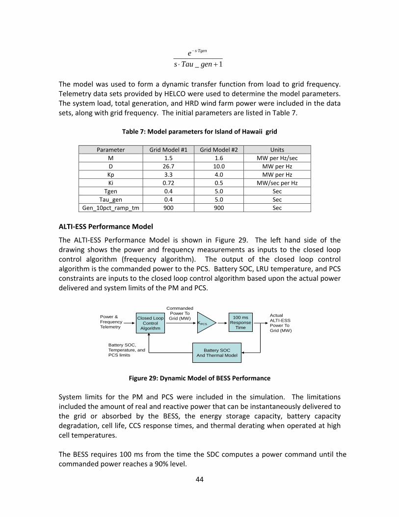
ALTI‐ESS Performance Model

The ALTI‐ESS Performance Model is shown in Figure 29. The left hand side of the drawing shows the power and frequency measurements as inputs to the closed loop control algorithm (frequency algorithm). The output of the closed loop control algorithm is the commanded power to the PCS. Battery SOC, LRU temperature, and PCS constraints are inputs to the closed loop control algorithm based upon the actual power delivered and system limits of the PM and PCS.

Closed LoopControl

AlgorithmKPCS

100 msResponse

Time

ActualALTI-ESSPower ToGrid (MW)

Battery SOCAnd Thermal Model

CommandedPower ToGrid (MW)Power &

FrequencyTelemetry

Battery SOC,Temperature, andPCS limits

Figure 29: Dynamic Model of BESS Performance

System limits for the PM and PCS were included in the simulation. The limitations included the amount of real and reactive power that can be instantaneously delivered to the grid or absorbed by the BESS, the energy storage capacity, battery capacity degradation, cell life, CCS response times, and thermal derating when operated at high cell temperatures. The BESS requires 100 ms from the time the SDC computes a power command until the commanded power reaches a 90% level.

45

Closed‐loop Control Algorithm Model

The Frequency Regulation Algorithm shown in Figure 24 consisted of four terms; frequency response, disturbance feed‐forward, battery SoC management, and power limit enforcement. The simulation determined the default values for the parameters. The results obtained from preliminary testing were used to further refine the default values. Key default parameters and their effects included the gain of the watts / Hz curve and the cut off frequency of the filter. The performance of the Frequency Regulation algorithm was assessed based upon the algorithm’s response to four disturbance inputs, two HELCO telemetry data sets, and Grid Model #1 and Grid Model #2. The parameters for Grid Model #1 and Grid Model #2 are listed in Table 8.

Table 8: Model Parameters for Grid Model #1 and Grid Model #2

Parameter Grid Model #1 Grid Model #2 Units

M 1.5 1.6 MW per Hz/sec

D 26.7 10.0 MW per Hz

Kp 3.3 4.0 MW per Hz

Ki 0.72 0.5 MW/sec per Hz

Tgen 0.4 5.0 Sec

Tau_gen 0.4 5.0 Sec

Gen_10pct_ramp_tm 900 900 Sec

The disturbance scenarios included: (1) Small Load Step Transient Response, (2) HRD Wind farm Step Transient Response, (3) Major Loss of Generation Transient Response, and (4) Steady State Variability. Each disturbance scenario is described in the following paragraphs. Transient Response Small Load Step disturbance scenario involved simulating the algorithm’s response to a 1 MW step increase in system load, while the HRD wind farm output was held constant. The performance metrics for this disturbance scenario include the maximum frequency excursion and the frequency recovery time. Transient Response HRD Wind Farm Step disturbance scenario involved simulating a 1 MW step reduction in power output from the HRD Wind Farm while system load was held constant. The performance metrics for this disturbance scenario include the maximum frequency excursion and the frequency recovery time. Transient Response Major Loss of Generation disturbance scenario involved simulating sudden loss of 10 MW of generation, while system load and HRD wind farm output were held constant. The performance metrics for this disturbance scenario included the maximum frequency excursion and the frequency recovery time.

46

Steady State Variability disturbance scenario involves driving the simulation using actual telemetry from the HELCO grid for system load and HRD wind farm output. The performance metric for this disturbance scenario is the control objective defined in Section 9.1. HELCO Telemetry Data sets included system load, total generation, HRD wind farm power, and system frequency. The telemetry data sets did not have any large‐scale loss of generation events. Instead, an artificially large value of 900 seconds was chosen to ensure the simulation would show behavior of the grid when the BESS is nearly depleted.

11.2. Wind Smoothing Algorithm

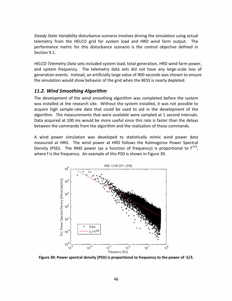
The development of the wind smoothing algorithm was completed before the system was installed at the research site. Without the system installed, it was not possible to acquire high sample‐rate data that could be used to aid in the development of the algorithm. The measurements that were available were sampled at 1 second intervals. Data acquired at 100 ms would be more useful since this rate is faster than the delays between the commands from the algorithm and the realization of those commands. A wind power simulation was developed to statistically mimic wind power data measured at HRD. The wind power at HRD follows the Kolmogorov Power Spectral Density (PSD). The RMS power (as a function of frequency) is proportional to f‐5/3, where f is the frequency. An example of this PSD is shown in Figure 30.

Figure 30: Power spectral density (PSD) is proportional to frequency to the power of ‐5/3.

47

The wind power simulation produces a realization of simulated data with a PSD that follows this Kolmogorov pattern while maintaining a mean value similar to what is typically found in the data. Simulated data sets typically run at a sampling rate of 10 Hz for a period of 24 hours. The first step in the simulation is to fit the Kolmogorov function to a target data set (real data at 1 Hz). A constant, when multiplied by f‐5/3, fits the target data. A re‐sampling technique was used to achieve the variation in power at various

frequencies. For example, to develop a realization of samples at 7 Hz, six Gaussian distributed samples are generated using a pseudo‐random number generator. These samples are interpolated to 864,000 samples (one day at 10 Hz) using a cubic spline interpolation algorithm. The mean of this set will be the inverse of the number of frequency points generated times the mean of the real data being modeled (after normalizing the component). The standard deviation is equal to the RMS power (divided

by the square‐root of the frequency) at 7 Hz. Using the re‐sampled data, the simulations show that the algorithm does succeed in smoothing the aggregate power produced by the HRD wind farm and BESS. Overall, the algorithm can eliminate PPA exceptions that would have occurred without the BESS. One of the features included in the algorithm (correction smoothing) did not add to the effectiveness and actually seems to have adverse effects. Also, certain combinations of the PID parameters can result in undesired results. Other PID parameter combinations result in less definitive conclusions. While a PID proportional gain of less than 50 seems to be ineffective, PID proportional gains between 50 and 100 are effective. Using a PID adder term that is too large (relative to the PID proportional gain) results in an effective 100% proportional response in a short time period.

12. Results of Laboratory Simulations

Section 12.1 presents the results of the acceptance tests for the laboratory simulations of the Frequency Regulation algorithm. The scenarios were used to verify the degree of compliance of the algorithm to the requirements and functional specifications. The following tests were conducted and the results presented in Section 12.1.

Transient response for a small load step

Transient response for a small HRD wind farm step

Transient response for a major loss of generation

Steady state variability Section 12.2 presents the results of the acceptance tests for the laboratory simulations of the Wind Smoothing algorithm. The scenarios were used to verify the degree of compliance of the algorithm to the requirements and functional specifications. The following tests were conducted and the results presented in Section 12.2.

48

Turn on

Turn off

Shut‐down in response to a loss of communication with battery power meter

Response to a low initial SOC

Response to a high initial SOC

Wind Disturbance Accuracy

12.1. Frequency Regulation Algorithm Simulation Results

The responses expressed in Recovery Times of the Frequency Regulation Algorithm to the three transient response test scenarios identified in Section 11 are listed in Table 9. The worst‐case frequency excursions in these scenarios are listed in Table 10. Recovery Time is defined as the time from beginning of the transient event until frequency reaches and remains above 59.985 Hz. OFF refers to the algorithm being set to inactive and ON refers to the algorithm being set to active.

Table 9: Recovery Time for Three Transient Response Test Scenarios

Grid Model #1 Grid Model #2

Closed Loop Control OFF ON OFF ON

Small Load Step 50 sec 6 sec 80 sec 60 sec

Wind Farm Step 50 sec 3 sec 80 sec 20 sec

Major Loss of Generation 860 sec 950 sec 900 sec 1000 sec

The results presented in the table indicate that Grid Model #1 produced better results in terms of shorter recovery times from the three input disturbances than the results for Grid Model #2. It can also be observed that the recover times with the frequency regulation algorithm set to active (ON) were shorter than the recover times with the frequency regulation algorithm set to in active (OFF). This was not true for the Major Loss of Generation test.

Table 10: Frequency Excursion for Three Transient Response Test Scenarios



Small Load Step 59.96 Hz 59.96 Hz 59.90 Hz 59.90 Hz

Wind Farm Step 59.96 Hz 59.96 Hz 59.90 Hz 59.90 Hz

Major Loss of Generation 59.63 Hz 59.63 Hz 59.00 Hz 59.01 Hz

The results presented in the table suggest that the results for Grid Model #1 and Grid Model #2 were essentially identical for all three input disturbances.

49

The steady state variability in frequency, RMS measurement in Hz at various timescales, is presented in Table 11. The test scenarios selected for the simulation included 1 sec, 3 sec, 10 sec, 100 sec, and 1000 sec timescales.

Table 11: Summary of Steady State Variability for Five Timescales



1 sec timescale 0.003 Hz 0.003 Hz 0.006 Hz 0.006 Hz





The results presented in the table suggest that the Steady State Variability with Grid Model #1 was in all but one case equal to or better with the frequency regulation algorithm set to active (ON) rather than set to inactive (OFF). Steady state variability with Grid Model #2 was worse for the 3 sec timescale and approximately equal to or better than for 1 sec, 10 sec, 100 sec, and 1000 sec timescales with the frequency regulation algorithm set to active (ON) rather than set to inactive (OFF). The 3 sec disturbance was noticeably worse. The figures that follow show the details of the results of the simulation for the three disturbance input test scenarios. In those figures the acronym PFR means Primary Frequency Regulation and the acronym DFF means Disturbance Feed Forward component of the Frequency Regulation Algorithm. In the final configuration of the Frequency Regulation algorithm the DFF component was set to inactive (OFF).

50

12.1.1. Small Load Step Transient Response Test Scenario Results

Figure 31: Small Load Step Transient Response Results ‐ Grid Model #1 (left figure) Grid Model #2 (right figure)

In Figure 31, the Blue trace is the results (transient response) from the simulation with the Frequency Regulation algorithm set to inactive (OFF) for a small load step. The Red trace is the results from the simulation with the Frequency Regulation algorithm set to active (ON) for a small load step. Note the oscillations and the time required to dampen the oscillations. The results observed in the figures suggest that Grid Model #2 recovers to 60 Hz in less than 400 sec while Grid Model #1 is slightly more than 400 sec for the small load step.

51

12.1.2. Wind Farm Step Transient Response Test Scenario Results

Figure 32: Wind Farm Step Transient Response ‐ Grid Model #1 (left figure) Grid Model #1 Detail (right figure)

In Figure 32, the Blue trace is the result (transient response using Grid Model #1) from the simulation with the Frequency Regulation algorithm set to inactive (OFF) for the wind farm step. The Red trace is with the Frequency Regulation algorithm set to active (ON). The right figure is a detailed view of the time starting at 0 sec and ending at 200 sec showing that the algorithm doesn’t oscillate above and below 60 Hz.

52

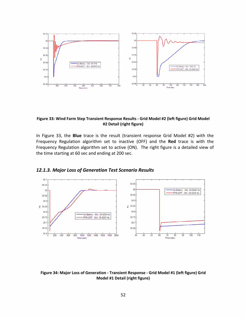
Figure 33: Wind Farm Step Transient Response Results ‐ Grid Model #2 (left figure) Grid Model #2 Detail (right figure)

In Figure 33, the Blue trace is the result (transient response Grid Model #2) with the Frequency Regulation algorithm set to inactive (OFF) and the Red trace is with the Frequency Regulation algorithm set to active (ON). The right figure is a detailed view of the time starting at 60 sec and ending at 200 sec.

12.1.3. Major Loss of Generation Test Scenario Results

Figure 34: Major Loss of Generation ‐ Transient Response ‐ Grid Model #1 (left figure) Grid Model #1 Detail (right figure)

53

In Figure 34, the Blue trace is the result (transient response Grid Model #1) with the Frequency Regulation algorithm set to inactive (OFF). The Red trace is the result (transient response) with the Frequency Regulation algorithm set to active (ON). The right figure is a detailed view of the time starting at 60 sec and ending at 120 sec. Note the frequency doesn’t recover to 60 Hz until approximately t = 1000 sec.

Figure 35: Major Loss of Generation Transient Response Results ‐ Grid Model #2 (left figure) Grid Model #2 Detail (right figure)

In Figure 35, the Blue trace is the result (transient response using Grid Model #2) with the Frequency Regulation algorithm set to inactive (OFF) and the Red trace is with the Frequency Regulation algorithm set to active (ON). The right figure is a detailed view of the time starting at 60 sec and ending at 190 sec. Note the frequency doesn’t recover to 60 Hz until approximately t = 1000 sec.

12.1.4. Steady State Steady State Variability in frequency and the RMS measurement in Hz at various timescales are presented in Table 12. The test scenarios selected for the simulation included 1 sec, 3 sec, 10 sec, 100 sec, and 1000 sec.

Table 12: Summary of Steady State Variability Results for Five (5) Timescales

54








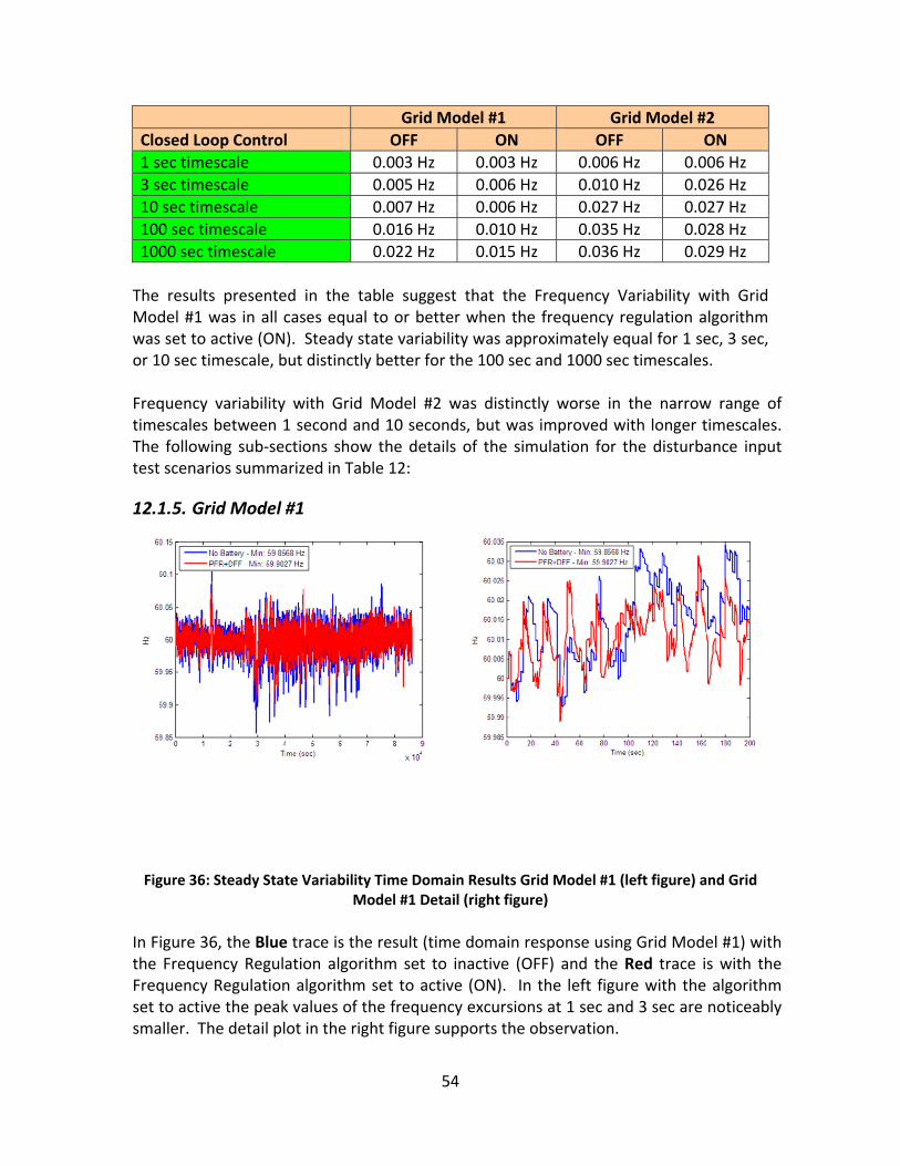
The results presented in the table suggest that the Frequency Variability with Grid Model #1 was in all cases equal to or better when the frequency regulation algorithm was set to active (ON). Steady state variability was approximately equal for 1 sec, 3 sec, or 10 sec timescale, but distinctly better for the 100 sec and 1000 sec timescales. Frequency variability with Grid Model #2 was distinctly worse in the narrow range of timescales between 1 second and 10 seconds, but was improved with longer timescales. The following sub‐sections show the details of the simulation for the disturbance input test scenarios summarized in Table 12:

12.1.5. Grid Model #1

Figure 36: Steady State Variability Time Domain Results Grid Model #1 (left figure) and Grid Model #1 Detail (right figure)

In Figure 36, the Blue trace is the result (time domain response using Grid Model #1) with the Frequency Regulation algorithm set to inactive (OFF) and the Red trace is with the Frequency Regulation algorithm set to active (ON). In the left figure with the algorithm set to active the peak values of the frequency excursions at 1 sec and 3 sec are noticeably smaller. The detail plot in the right figure supports the observation.

55

Figure 37: Stead State Variability Results for Five Timescales ‐ Grid Model #1

In Figure 37, the Blue trace is the RMS with the Frequency Regulation algorithm set to inactive (OFF) and the Black trace is with the Frequency Regulation algorithm set to active (ON). The thicker, solid Black trace is the control target. In this scenario the control target is mostly above the desired RMS.

12.1.6. Grid Model #2

Figure 38: Steady State Variability Time Domain Results ‐ Grid Model #2 (left figure) and Grid Model #2 Detail (right figure)

56

In Figure 38, the Blue trace is the result (time domain response using Grid Model #2) with the Frequency Regulation algorithm set to inactive (OFF) and the Red trace is with the Frequency Regulation algorithm set to active (ON).

Figure 39: Steady State Variability for Five Timescales ‐ Grid Model #2 (left figure) and Grid Model #2 Detail (right figure)

In Figure 39, the Blue trace is the RMS measurement with the Frequency Regulation algorithm set to inactive (OFF) and the Black trace is with the Frequency Regulation algorithm set to active (ON). The thicker, solid Black trace is the control target. In this scenario the control target is mostly below the desired RMS.

12.2. Wind Smoothing Algorithm Simulation Results

Figure 40 is a simplified model of the algorithm used for the simulations. The model has two control inputs and one raw wind power (in kW) disturbance input. The SOC reference is a configurable parameter and is selectable using the PM HMI. The Actual Battery SOC refers to the SOC value provided by the BMS and is based upon the open circuit voltage of each cell group. During the tests, the term OFF refers to the algorithm being set to inactive and the term ON refers to the algorithm being set to active.

57

Figure 40: Overview of Wind Smoothing Algorithm

Figure 41 shows the simulation test results for the wind smoothing algorithm with time constants of 20 seconds (Green), 60 seconds (Blue), and 90 seconds (Grey). The red trace is the raw wind power. The vertical axis is wind farm power in kW.

Figure 41: Smoothing of 20 (green), 60 (blue), and 90 (grey) seconds (2 Hour Span)

Even at this 2‐hour time scale, it is apparent that the strongest fluctuations occur when the algorithm is not running (Red trace).

58

Figure 42 shows an expansion at the 15‐minute time scale. It is notable that time constants of 60 and 90 seconds greatly outperform the 20 second value.

Figure 42: Smoothing of 20 (green), 60 (blue), and 90 (grey) seconds (15 Minute Span)

Figure 43 is a plot of the results of the simulations using the cycling (Turn On / Turn Off) test protocol. From the PM HMI the Wind Smoothing control strategy was selected and the algorithm set to active. The duration of the test was 200 seconds. The vertical axis is wind power in kW. The upper Red trace in the figure shows the maximum power that can be sourced and the corresponding ramp rate limits. The lower Red shows the maximum power that can be synced and the corresponding ramp rate limits. The Blue trace is a plot of the commanded power level during the test.

59

Figure 43: Turn On / Turn Off Simulation Acceptance Test Results

Figure 44 is a plot of the results of the simulation for a Loss of Communication with the PM meter. Utilizing the HMI the wind smoothing control strategy (algorithm) was set to active (ON). The test scenario simulated the loss of communication with the PM meter which caused the CCS to issue a 0.00 kW power command. Under this condition, the CCS would not be receiving frequency, voltage, power, and current data from the PM meter to run the algorithm until restoration of communications. With no input data the BESS was taken off line until communication was restored. The algorithm responded per the requirements and functional specifications. The duration of the test was 240 seconds.

Figure 44: Response to a Loss of Communication with PM SEL 735P

Figure 45 is a plot of the results of the simulation for a Loss and Restoration of Communication with the Totalizer SEL 735P meter. The test scenario simulated the loss of communication with the Totalizer meter which caused the CCS to continue normal operation. The algorithm responded per the requirements and functional specifications. The duration of the test was 170 seconds.

60

Figure 45: Response to a Loss and Restoration of Communication with Totalizer SEL 735P

Figure 46 is a plot of the results of the simulation of a Loss of Communication with the Wind Power meter. Utilizing the HMI, the wind smoothing control strategy (algorithm) was set to active (ON). The test scenario simulated the loss of communication with the Wind Power meter which caused the CCS to ramp the output power to 0kW over a predetermined amount of time and held at that value until communication with the Wind Power meter was restored. The duration of the test was 200 seconds. The algorithm responded per the requirements and functional specifications.

Figure 46: Response to a Loss of Communication with Wind Power SEL 735P

Figure 47 is a plot of the results of the simulation of a Low Initial SOC test. Utilizing the HMI the wind smoothing control strategy (algorithm) was set to active and the output power level was held constant starting with a 20% SOC. The duration of the test was 75 minutes. The test scenario results reached a steady state value of 48% in 60 minutes. The algorithm responded per the requirements and functional specifications.

61

Figure 47: Response to a Low Initial SOC

Figure 48 is a plot of the results of the High Initial SOC acceptance test. Utilizing the HMI the wind smoothing control strategy (algorithm) was set to active and the output power level was held constant starting with an 80% SOC. The duration of the test was 68 minutes. The test scenario results reached a steady state value of 50.5% in 41 minutes. The algorithm responded per the requirements and functional specifications.

Figure 48: Response to a HIGH Initial SOC

Figure 49 is a plot of the results of the simulation of the Wind Disturbance Accuracy test. The simulation used wind farm data sets. The initial test failed to meet the stated requirement of 98% of the time the difference between the power command and the power correction will be less than 20 kW.

62

Figure 49: Response to a HIGH Initial SOC

The root cause was determined and corrective action taken. The simulations were not rerun and verification was left to the formal acceptance testing at the Research site.

13. Conclusion This report presented the technical work completed under Subtask 3.2, text Item 3.2.2 "Control Algorithms", conducted under Award Number DE‐EE0003507, Hawaii Energy Sustainability Program (HESP). The scope of Subtask 3.2 (Item 3.2.2), included investigating the effectiveness of real‐time control algorithms to control a relatively small, but fast‐acting BESS to reduce undesirable effects of high‐penetrations of renewable resources onto the electric grid by responding to grid frequency, or by responding to fluctuations in wind power generated at Hawi on the north shore of the Island of Hawaii . During the period between July, 2010 and October, 2012, with funding under an ONR grant, the fast‐acting ALTI‐ESS was manufactured, tested, and delivered to the Hawi Wind Farm research site. The ALTI‐ESS was unpacked, re‐assembled, and grid‐connected to the HELCO electric grid in November, 2012. During the period between January, 2012 and November, 2012, HNEI (with funding from this DOE grant) provided technical oversight and assistance to a team, made up of both public and private entities, to develop and integrate the frequency regulation and wind smoothing algorithms needed to control the BESS. In December, 2012 preliminary testing of the two control algorithms verified that with either control algorithm set to active that no erroneous power commands were issued by the SDC.

63

Commissioning and final acceptance testing of the BESS with the two control algorithms started in January, 2013. The preliminary results of the analysis of the Frequency Regulation algorithm presented in Figure 50 started in March, 2013.

Figure 50: Preliminary Results of Frequency Regulation Algorithm

The vertical axis of the top plot in the figure is BESS power in kW. The vertical axis of the middle plot in the figure is HELCO grid frequency in Hz. The vertical axis for the bottom plot is wind power in MW. The horizontal axis is time of day for both plots. The test started at 4:00:00 PM and ended at 7:20:00 PM. The test was divided into five 40 minute periods; each period included 20 minutes with the algorithm set to active (ON) and 20 minutes with the algorithm set to inactive (OFF). In both plots, the Black trace indicates the BESS was inactive, and the Red trace indicates the BESS was active. Note the qualitative results (effect of algorithm) shown in the bottom plot. The variability in the red portions of the plot for each period is noticeable smaller compared to the black portions of the plot for all five periods. The typical reduction in grid frequency variability is between 30% and 40%.

64

Wind smoothing analysis presented in Figure 51 started in Aril, 2013. The figure consists of four plots of the performance of the Wind Smoothing algorithm using data from April, 2013.

Figure 51: Preliminary Results of Wind Smoothing Algorithm

The vertical axis in all four plots in the figure is power in kW. The horizontal axis is time in minutes. The test started at 8:00:00 AM and ended 600 minutes later. The plot at the top of the figure shows the raw wind power (Black trace) and smoothed wind power (Red Trace) meaning the sum of the raw wind power and the BESS power. Note the qualitative results (effect of algorithm) shown in the figure. The red trace is noticeable smoother and lacks the sharp features when compared to the black trace. The preliminary results presented here support the conclusions drawn from the original simulations. A robust research plan is being developed under ONR funding to complete the analysis and validation of the BESS, grid, and algorithm performance. Data will be collected and analyzed over the next two years.

65

Works Cited [1] K. Musser, "Closed Loop Control Algorithm Requirements and Functional

Specification: Frequency Regulation". Rev 5, 13‐August, 2012. [2] H. Logan, "Closed Loop Control Algorithm Requirements and Functional

Specification: Wind Smoothing". Rev 5, 10‐August, 2012. [3] K. Musser, "Closed Loop Control Algorithm System Architecture and HMI Report:

Frequency Regulation". 31‐August, 2012. [4] H. Logan, "Closed Loop Control Algorithm System Architecture and HMI Report:

Wind Smoothing". Rev 11, 18‐August, 2012. [5] K. Musser, "Closed Loop Control Algorithm Simulation Results Report: Frequency

Regulation". Rev 3, 25‐September, 2013. [6] H. Logan, "Closed Loop Control Algorithm Simulation Results Report: Wind

Smoothing". Rev 8, 28‐December, 2012. [7] K. Musser, "Closed Loop Control Algorithm Lab Acceptance Test Plan: Frequency

Regulation". Rev 6, 6‐August, 2013. [8] K. Musser, "Closed Loop Control Algorithm Lab Acceptance Test Plan: Wind

Smoothing". Rev 2, 6‐August, 2013. [9] K. Musser, "Closed Loop Control Algorithm Lab Acceptance Test Results:

Frequency Regulation". Rev 1, 1‐March, 2013. [10] K. Musser, "Closed Loop Control Algorithm Lab Acceptance Test Results: Wind

Smoothing". Rev 6, 15‐April, 2013. [11] K. Musser, "Closed Loop Control Algorithm Site Acceptance Test Results:

Frequency Regulation". Rev 3, 19‐February, 2013. [12] K. Musser, "Closed Loop Control Algorithm Site Acceptance Test Results: Wind

Smoothing". Rev 1, 15‐April, 2013.

Development of Real-time Closed-loop Control Algorithms ... · Development of Real-time Closed-loop...

Documents

Transcript of Development of Real-time Closed-loop Control Algorithms ... · Development of Real-time Closed-loop...