Anyons in dimensions and the deformed Calogero …420111/FULLTEXT02.pdf · Anyons in (1+1)...
98
Anyons in (1 + 1) dimensions and the deformed Calogero-Sutherland model Farrokh Atai Master of Science Thesis Department of Theoretical Physics Royal Institute of Technology Stockholm 2011
Transcript of Anyons in dimensions and the deformed Calogero …420111/FULLTEXT02.pdf · Anyons in (1+1)...
Anyons in (1 + 1) dimensions andthe deformed Calogero-Sutherland
model
Farrokh Atai
Master of Science Thesis
Department of Theoretical PhysicsRoyal Institute of Technology
Stockholm 2011


Master of Science Thesis
Anyons in (1 + 1) dimensions and thedeformed Calogero-Sutherland model
Farrokh Atai
Mathematical Physics, Department of Theoretical PhysicsRoyal Institute of Technology, SE-106 91 Stockholm, Sweden
Stockholm, Sweden 2011

Typeset in LATEX
Examensarbete inom amnet fysik for avlaggande av civilingenjorsexamen
Graduation thesis on the subject Physics for the degree of Master of Science inEngineering
TRITA-FYS 2011:16ISSN 0280-316XISRN KTH/FYS/--11:16--SE
c© Farrokh Atai, May 2011Printed in Sweden by Universitetsservice US AB, Stockholm 2011

Abstract
This thesis deals with a conformal field theoretical treatment of abelian anyons in(1+1)-dimensions and their relation to the integrable Calogero-Sutherland models.We generalize previous work relating anyons to the Calogero-Sutherland model byshowing that the correlation function of the anyon field operators corresponds tothe eigenfunctions of the deformed Calogero-Sutherland model. Our results suggesta physical application of the deformed Calogero-Sutherland model in the contextof the fractional quantum Hall effect (FQHE).
A key aspect for this work is the introduction of the dual anyon field operators,which obey a natural generalization of the canonical anti-commutation relation.
Key words: FQHE, Anyons, Integrable many-body system,Deformed Calogero-Sutherland model
Sammanfattning
Denna avhandling behandlar abelska anyoner, med hjalp av konform faltteori, i(1 + 1)-dimensioner och deras relation till de fullt losbara Calogero-Sutherlandmodellerna. Vi visar att anyon faltoperatorernas korrelationsfunktion motsvararegenfunktionerna av den deformerade Calogero-Sutherland modellen, vilket ar engeneralisering av tidigare arbete kring anyonernas relation till Calogero-Sutherlandmodellen. Vara resultat tyder pa en fysisk tillampning av den deformerade Calogero-Sutherland modellen i samband med den fraktionerade kvanthalleffekten (FQHE).
En viktig aspekt for detta arbete ar inforandet av dual anyon operatorn, somuppfyller en naturlig generalisering av den kanoniska anti-kommuteringsrelation.
iii

iv

Contents
Abstract . . . . . . . . . . . . . . . . . . . . . . . . . . . . . . . . . . . . iiiSammanfattning . . . . . . . . . . . . . . . . . . . . . . . . . . . . . . . iii
Contents v
Introduction ix
Summary of results xiii
1 Preliminaries 11.1 Introductory explanations . . . . . . . . . . . . . . . . . . . . . . . 1
1.1.1 Second quantization maps . . . . . . . . . . . . . . . . . . . 21.2 Normal ordering . . . . . . . . . . . . . . . . . . . . . . . . . . . . 5
1.2.1 Fermion normal-ordering . . . . . . . . . . . . . . . . . . . 51.2.2 Boson normal-ordering . . . . . . . . . . . . . . . . . . . . . 6
1.3 Many-body operators . . . . . . . . . . . . . . . . . . . . . . . . . 61.3.1 Operators of interest . . . . . . . . . . . . . . . . . . . . . . 61.3.2 Formal field operators . . . . . . . . . . . . . . . . . . . . . 71.3.3 Operator regularization . . . . . . . . . . . . . . . . . . . . 8
1.4 Formal distributions . . . . . . . . . . . . . . . . . . . . . . . . . . 81.4.1 Preliminaries . . . . . . . . . . . . . . . . . . . . . . . . . . 91.4.2 Formal delta-function . . . . . . . . . . . . . . . . . . . . . 9
1.5 Baker-Campbell-Hausdorff formulas . . . . . . . . . . . . . . . . . 11
2 Anyons in (1 + 1) dimensions 132.1 Boson-fermion correspondence . . . . . . . . . . . . . . . . . . . . . 132.2 Boson-anyon correspondence . . . . . . . . . . . . . . . . . . . . . 152.3 Dual anyon operators . . . . . . . . . . . . . . . . . . . . . . . . . 17
3 Anyons and the CS model 213.1 The Calogero-Sutherland type model . . . . . . . . . . . . . . . . . 21
3.1.1 The CS model . . . . . . . . . . . . . . . . . . . . . . . . . 223.1.2 Relation to the Laughlin state . . . . . . . . . . . . . . . . 22
v

vi Contents
3.1.3 The deformed Calogero-Sutherland model . . . . . . . . . . 233.2 The Hν,s operators . . . . . . . . . . . . . . . . . . . . . . . . . . . 24
3.2.1 Construction of the anyon differential operators . . . . . . . 243.2.2 The duality of species ν and −1/ν . . . . . . . . . . . . . . 263.2.3 The groundstate eigenvector . . . . . . . . . . . . . . . . . . 28
3.3 Anyons relation to the CS model . . . . . . . . . . . . . . . . . . . 29
4 Anyons and the dCS model 334.1 Anyons and the dCS differential operator . . . . . . . . . . . . . . 334.2 Anyons and the dCS eigenfunctions . . . . . . . . . . . . . . . . . . 34
5 Conclusions 37
Acknowledgements 39
A Summary of notations 41
B Boson normal-ordering relations 43B.1 Normal-ordering products of Q’s and R’s . . . . . . . . . . . . . . 43B.2 Normal-ordering products of anyon operators of arbitrary number 44
B.2.1 Product with the same species. Proof of Lemma 2.3.4 . . . 44B.2.2 Products of different species. Proof of Lemma 2.3.5 . . . . 47
C Fock space equality 49C.1 Boson completeness . . . . . . . . . . . . . . . . . . . . . . . . . . 49
D The W -current 53D.1 The W1+∞ algebra . . . . . . . . . . . . . . . . . . . . . . . . . . . 53D.2 The Sugawara construction . . . . . . . . . . . . . . . . . . . . . . 56D.3 The anyon W -current . . . . . . . . . . . . . . . . . . . . . . . . . 57
D.3.1 Construction of the W ν,s operator . . . . . . . . . . . . . . 58D.3.2 The W ν,s relations . . . . . . . . . . . . . . . . . . . . . . . 59
E Additional proofs 63E.1 Proofs for Chapter 1 . . . . . . . . . . . . . . . . . . . . . . . . . . 63
E.1.1 Proof of Proposition 1.4.4 . . . . . . . . . . . . . . . . . . . 63E.1.2 Proof of Lemma 1.5.1 . . . . . . . . . . . . . . . . . . . . . 64
E.2 Proofs for Chapter 2 . . . . . . . . . . . . . . . . . . . . . . . . . . 64E.2.1 Proof of Proposition 2.1.2 . . . . . . . . . . . . . . . . . . . 64E.2.2 Proof of Lemma 2.2.4 . . . . . . . . . . . . . . . . . . . . . 65E.2.3 Proof of Proposition 2.3.2 . . . . . . . . . . . . . . . . . . . 65
E.3 Proofs for Chapter 3 . . . . . . . . . . . . . . . . . . . . . . . . . . 66E.3.1 Proof of Lemma 3.2.4 . . . . . . . . . . . . . . . . . . . . . 66E.3.2 Proof of Lemma 3.3.2 . . . . . . . . . . . . . . . . . . . . . 67E.3.3 Proof of Lemma 3.3.3 . . . . . . . . . . . . . . . . . . . . . 68

Contents vii
E.3.4 Proof of Corollary 3.3.6 . . . . . . . . . . . . . . . . . . . . 69E.4 Proofs for Chapter 4 . . . . . . . . . . . . . . . . . . . . . . . . . . 70
E.4.1 Proof of Theorem 4.1.2 . . . . . . . . . . . . . . . . . . . . 70E.4.2 Proof of Theorem 4.2.1 . . . . . . . . . . . . . . . . . . . . 74E.4.3 Proof of Corollary 4.2.2 . . . . . . . . . . . . . . . . . . . . 74
Bibliography 77

viii

Introduction
“ The motivation for a physicist to study 1-dimensional problems is bestillustrated by the story of the man who, returning home late at nightafter an alcoholic evening, was scanning the ground for his key undera lamppost; he knew, to be sure, that he had dropped it somewhereelse, but only under the lamppost was there enough light to conduct aproper search.” -F. Calogero [1]
Much has changed since this statement was published in 1970. One dimensionalsystems are, today, a reality for those dealing with experimental condensed matterphysics and have produced some very interesting physical results, such as carbonnanotubes.
The 1-dimensional problems of particular interest are those described by ex-actly solvable models (integrable systems). Integrable systems play an importantrole as they provide an exact solutions that offers insight into properties whichmight not be gotten from approximations. Integrable models are also used asknown solutions from which physicist start using approximative methods, such asperturbation theory. Integrable models are, therefore, essential as they provide atheoretical basis for our physical reality or, at least, act as a starting points forknown unknowns. In this thesis certain integrable models play an important role,namely the original Calogero-Sutherland (CS) model [2] [3] and the generalization ofthe Calogero-Sutherland model known as the deformed Calogero-Sutherland (dCS)model [4] [5] [6].
A motivation for this work is the fractional quantum Hall effect (FQHE) dis-covered in 1982 by Tsui et al. [7]. The FQHE corresponds to plateaus in the Hallconductivity of two-dimensional electron systems subject to very low temperaturesand extremely high magnetic fields. For the integer QHE the plateau region isquantized into positive integer, νfill, which is commonly referred to as the fillingfactor,1 multiples of the inverse von Klitzing constant (R−1
K = (h/e2)−1) and isexplained as the manifestation of a single particle phenomena (see e.g. [8] and thereferences therein).
1In the bulk of the thesis the parameter ν will represent the statistical parameter of the anyonsand should not be confused with the filling factor νfill.
ix

x Introduction
In the FQHE the quantum number νfill can take the value of a positive rationalnumber instead of a positive integer. This was observed only in samples withhigh mobility and it was concluded that the effect must be related to the electron-electron interaction, rather than being a single electron phenomena. A successfulapproximation for the groundstate wavefunction was done by R. Laughlin in 1983[9], which corresponded to a filling factor of one over a odd positive integer (νfill =1/ (2m+ 1)). The wavefunction described a circular droplet of condensed two-dimensional electron gas into an incompressible liquid known as a quantum Hall(QH) liquid. The Laughlin wavefunction also incorporated that each electron hasprecisely 2m pinned magnetic vortices attached to it. Simulations done by Laughlin,in the same paper, showed that the wavefunction corresponded to the observationsof Tsui et al. for νfill = 1/3.
A similar treatment was made by Haldane and Halperin (HH) [10] [11] for fillingfractions not explained by the Laughlin wavefunction as the superposition of quasi-particles and quasi-holes creating ”daughter” states from the existing ”parent”states, starting from the Laughlin νfill = 1/3 state, put on a spherical surface witha magnetic monopole at origo.
An alternative approach was given by Jain [12] for the νfill = p/(2mp ± 1)plateaus, where m and p are positive integers, by the construction of compositefermions, i.e. fermions bound to a flux tube, and explained the FQHE as a man-ifestation of the integer QHE with composite fermions. The method presented byJain had the advantage of being simpler than the HH approach, while simultane-ously predicting the stability of filling factors and thereby new fractions that werebound to appear. The method does not explain all the observed QH fractions as itpredicts fractions with odd denominators only.
Topological field theory (the celebrated Chern-Simons theory [13]) indicatesthat the low-energy excitations of the boundary states play a crucial role in theFQHE [14] [15]. By restricting the Laughlin wavefunction to the boundary, theCalogero-Sutherland groundstate is obtained with a shift in the center of mass(CoM) energy (c.f. Section 3.1.2). It was later discovered that the particles wherequasi-particles exhibiting not just bosonic and fermionic statistics, but a new typeof particle statistics which interpolates between bosonic and fermionic [16]. Thequasi-particles were named anyons [17],2 since they can gain any phase shift duringexchange. It is known that there is a direct connection between the Calogero-Sutherland type models and anyons in 1+1 dimensions [18] [19] and the FQHE [20].A recent renewed high level of interest in this topic is sparked by the existence ofnon-abelian anyonic, topological states found in the QH states at νfill = 5/2, whichcan be used in the creation of topological quantum computers [21].
This thesis is a generalization of the work by E. Langmann and A. Carey [19],which introduced the anyon field operators using the boson-fermion correspondencein (1 + 1)-dimensions (references on earlier work in this direction are discussedin [19]). They also showed the explicit construction of an self-adjoint anyonic
2Not to be confused with anions.

xi
operator Hν,3 corresponding to the second quantization of the Calogero-SutherlandHamiltonian (c.f. Section 3.2). This thesis will continue by introducing a newtype of anyonic field operator, corresponding to an dual anyon. Further on, onecan show that the correlation functions of these operators, combined with previousanyon operators, correspond to solutions of the dCS model. We will also showthat the self-adjoint operator Hν,3, introduced in [19], will give the dCS differentialoperator when acting upon a vector created by the many-body anyon and dualanyon field operators. This allows to naturally interpret the Hν,3 operator as thesecond quantization of the dCS differential operator.
Outline of thesis
At first, an informal summary of the results is provided, avoiding the technicalitiesof the main text.
Chapter 1 will introduce the basic concepts and the mathematical objects usedin this thesis and their relations. It is recommended that readers unfamiliar withthe subject skim through Chapter 1 briefly before reading the rest.
In Chapter 2, the boson-fermion correspondence will be discussed and extendedin order to construct anyon field operators in (1 + 1)-dimensions. Finally, the dualanyon field operator is introduced, and we show that the anyon and dual anyon fieldoperators obey a generalization of the canonical anti-commutation relation (CAR),and that they have other interesting algebraic relations.
Chapter 3 gives a brief introduction to the Calogero-Sutherland (CS) and thedeformed Calogero-Sutherland (dCS) models. We then explicitly show the con-struction of a self-adjoint operator corresponding to the second quantization of thedCS differential operator and its relation to the anyon operators. We also showthat the expectation value of these operators give the CS Hamiltonian and the CSgroundstate wavefunction (up to a constant factor and a center of mass (CoM)shift).
In Chapter 4 a new eigenvector of the second quantized dCS differential opera-tor will be constructed by using the anyon and dual anyon field operators. Thenwe show that the expectation value of the Hν,3 operator and this new eigenvectorcorresponds to the dCS differential operator and the deformed groundstate eigen-function, up to a constant and a CoM shift. Using this result, a general methodfor constructing eigenfunctions of the dCS differential operator is obtained.
Throughout the thesis, all proofs that require mathematical calculations are putinto appendices B-E. Appendix A contains a summery of the most common nota-tions used throughout this thesis.

xii

Summary of results
In this Section a brief and compact summary is given that does not include thetechnicalities of the main text of this thesis. The result of the summary is obtainedfrom the results in the main text for the formal distributions in a suitable distribu-tional sense. See Appendix A for details on the notations used.
Summary
The Calogero-Sutherland model is a quantum mechanical model describing N ∈ Nindistinguishable particles on a circle with circumference L > 0, which we denoteby SL, via a translationally invariant, inverse quadratic potential. The Calogero-Sutherland model is defined by the Hamiltonian
HN := −N∑k=1
∂2
∂x2k
+ 2λ (λ− 1)∑k′<k
V (xk − xk′) (1)
where
V (r) :=π2
L2
1
sin2(πL (r)
)and xk ∈ SL is such that xk > xk′ for all k > k′.
The CS model has the groundstate (GS) wavefunction
ψ0(x) :=∏k′<k
(sin(πL
(xk − xk′)))λ
(2)
where ψ0(x) ∈ L2(SNL ) for λ ≥ − 12 , and corresponds to an eigenvalue of
E0 :=π2λ2N
(N2 − 1
)3L2
The CS model has exact eigenfunctions of the form
Ψn(x) = Pn,λ(w)ψ0(x)
where Pn,λ(w) are polynomials which are invariant under permutations of particle
coordinates, labeled by partitions n := (n1, n2, . . . , nN ) ∈ NN , and wk := e2πL ixk .
xiii

xiv Summary of results
The deformed Calogero-Sutherland (dCS) model is defined by the differentialoperator
HN,M := −N∑k=1
∂2
∂x2k
+ λ
M∑j=1
∂2
∂y2j
+ 2 (1− λ)
N∑k=1
M∑j=1
V (xk − yj)
+ 2λ (λ− 1)∑k′<k
V (xk − xk′) +2 (λ− 1)
λ
∑j′<j
V (yj − yj′) (3)
where yj ∈ SL for all j = 1, 2, . . . ,M such that yj > yj′ for j > j′, and xk 6= yj forall j, k.
The dCS differential operator has exact eigenfunctions which are similar to theexact eigenfunctions of the CS Hamiltonian. The eigenfunction corresponding toψ0(x) is denoted by ψ0(y,x), which we refer to as the deformed groundstate (dGS)eigenfunction, and is defined as
ψ0(y,x) :=∏k′<k
sinλ(πL
(xk − xk′))∏j′<j
sin1λ
(πL
(yj − yj′)) N∏k=1
M∏j=1
1
sin(πL (xk − yj)
)The eigenvalue of the dCS differential operator corresponding to ψ0(y,x) is
E0 :=π2
3L2
(Nλ−M) (Nλ− λ−M) (Nλ+ λ−M)−M(λ2 − 1
)λ
Abelian anyons are quantum particles which are characterized by their particleexchange relation where they can obtain any phase shift. Anyon quantum fieldoperators would be characterized by the relation
φ1(x)φ2(y) = e±iϑφ2(y)φ1(x) for x ≶ y, x, y ∈ SL , x 6= y
with a phase ϑ ∈ R. Thus the anyons become bosonic if ϑ = 2πn or fermionic ifϑ = π (2n+ 1) where n ∈ Z.
Starting from the boson-fermion correspondence in (1 + 1) dimensions, there isa generalization which allows us to construct field operators satisfying the exchangerelation for abelian anyons [19]. The formal anyon field operators are denoted byφν(x), where ν is the statistical parameter3 of the anyon field operators, and obey4
φν(x) = φ−ν(x)∗
φν(x)φν′(y) = e−iπνν
′sgn(x−y)φν′(y)φν(x) , x 6= y, x, y ∈ SL
where πνν′ ∈ R. Our construction of the anyon field operators require that thestatistical parameter of the anyon field operator is an integer times an arbitrary
3The statistical parameter ν is not the filling factor for the fractional quantum Hall effect.4We will denote complex conjugation and Hermitian conjugate by ∗

xv
constant ν0 ∈ R \ 0 (c.f. Section 2.2).
By generalizing the construction of the fermion W -algebra to anyons, we con-struct an operator valued generating function for the anyon differential operators(c.f. Appendix D.3) and thereby construct the anyon differential operators up tosecond order and their relations (c.f. Section 3.2).
The second quantization of the dCS differential operator is denoted by Hν,3(given by Eq. (3.20)) and is a self-adjoint operator obeying the highest weightcondition
Hν,3Ω = 0 , ∀ νwhere Ω denotes the vacuum vector in the Fock space F (c.f. Section 1.1).
The anyon field operators and the Hν,3 operator obey the commutation relation[Hν,3, φν(x)
]Ω = − ∂2
∂x2φν(x)Ω
The commutation relation holds for all ν as long as the Hν,3 operator and anyonfield operator have the same statistical parameter.
The zeroth order anyon differential operator is denoted by Hν,1 and obeys
Hν,1Ω = 0[Hν,1, φ±ν(x)
]= ±φ±ν(x)
The Hν,3 operator can be interpreted as the charge operator for anyons withstatistical parameter ν.
Let Φν(x) denote the product of N ∈ N anyon field operators, i.e.
Φν(x) := φν(x1)φν(x2) · · ·φν(xN )
where x := (x1, x2, . . . , xN ) ∈ SNL is such that xk > xk′ for all k > k′.The Hν,3 operator and the many-body anyon field operator Φν(x) obey the
commutation relation[Hν,3,Φν(x)
]Ω =
(−
N∑k=1
∂2
∂x2k
+ 2ν2(ν2 − 1
) ∑k′<k
V (xk − xk′)
)Φν(x)Ω (4)
Comparing Eq. (4) to Eq. (1), we see that the commutation relation yields theCS Hamiltonian for λ = ν2. The Hν,3 operator can therefore be interpreted as thesecond quantization of the CS Hamiltonian.
Let η be an eigenvector of the Hν,3 operator, belonging to a dense, invariantdomain, with eigenvalue E . Then the function Fη(x), defined as
Fη(x) := 〈η,Φν(x)Ω〉
is an eigenfunction of the CS Hamiltonian with eigenvalue E , since⟨η,Hν,3Φν(x)Ω
⟩= HN 〈η,Φν(x)Ω〉
We show in Section 3.3 that there exist a eigenvector ηCS, which corresponds tothe GS wavefunction of the CS model, up to a constant and with a center of mass

xvi Summary of results
(CoM) shift (c.f. Corollary 3.3.6).
We introduce φ−1ν (y) (c.f. Eq. (2.19)) and postulate that the φ−
1ν operator
corresponds to the dual anyon field operator to an anyon field operator with sta-tistical parameter ν. The dual anyon field operator is a well-defined field operatorif and only if 1
νν0∈ Z, where ν0 is the same constant used in the construction of
the anyon field operators. The anyon and the dual anyon field operators obey (c.f.Eqs. (2.20) and (2.22))
φν(x), φ−1ν (y)
= Lδ(x− y)φ(ν− 1
ν )(x)
where δ(x) is the Dirac delta and the factor of L is due to the fact that the anyonoperators are dimensionless.
The second quantization of the CS Hamiltonian has an interesting duality forthe operators with statistical parameter ν and −1/ν given by
Hν,3 = −ν2H− 1ν ,3 +
π
3L2
(ν4 − 1
)ν2
H− 1ν ,1
So it is possible to create eigenvectors of the Hν,3 operator by using the dual anyonoperator.
These two relations support the notion that the dual operator for an anyon fieldoperator φν has to be φ−
1ν rather than the conjugate φ−ν .
Let ϕν(y,x) denote the product of M ∈ N dual anyon field operators and N ∈ Nanyon field operators, i.e.
ϕν(y,x) := Φ−1ν (y)Φν(x)
where y := (y1, y2, . . . , yM ) ∈ SML is such that yj > yj′ for all j > j′ and xk 6= yjfor all k, j.
The operator ϕν(y,x) and the Hν,3 operator obey the commutation relation(c.f. Theorem 4.1.2)
[Hν,3, ϕν(y,x)
]Ω =
(HN,M +
π2
3L2
ν4 − 1
ν2M
)ϕν(y,x)Ω (5)
where HN,M is the dCS differential operator for λ = ν2.Equation (5) allows the construction of eigenfunctions of the dCS differential
operator (c.f. Theorem 4.2.1), which is as follows.Let η be an eigenvector of the Hν,3 operator, with eigenvalue E , and belong to
an dense, invariant domain. Then there exists a function Fη(y,x) defined as
Fη(y,x) := 〈η, ϕν(y,x)Ω〉

xvii
which5 is an eigenfunction of the dCS differential operator with eigenvalue
HN,M Fη(y,x) =
(E − π2
3L2
ν4 − 1
ν2M
)Fη(y,x)
Creating η vector corresponding to the exact solutions of the dCS model isoutside the scope of this thesis. We restrict ourselves to the simplest possibleeigenvector, η0, for now.
The Fock space inner product of a vector created by the ϕν(y,x) field operatorand the η0 vector is denoted by
〈η0, ϕν(y,x)Ω〉 = F0(y,x)
where F0(y,x) is given by (c.f. Section 4.2 or Corollary 4.2.2)
F0(y,x) := κ ψ0(y,x) e−iπ(Nν2−M)
Lν2
(ν2
N∑k=1
xk−M∑j=1
yj
)
where
ψ0(y,x) :=∏j′<j
sin1ν2
(πL
(yj − yj′)) ∏k′<k
sinν2(πL
(xk − xk′)) N∏k=1
M∏j=1
1
sin(πL (xk − yj)
)and κ ∈ C is a constant. The correlation function equals the dGS eigenfunction ofthe dCS differential operator, up to a constant and a CoM shift, for λ = ν2. Weshow that this is indeed the case where the eigenvalue corresponds to the eigenvalueof the dGS eigenfunction with a CoM shift contribution (c.f. Section 4.2).
5It is assumed that the η vector is not orthogonal to the vector created by the many-bodyoperator ϕν(y, z).

xviii

Chapter 1
Preliminaries
There are several important notations that have to be explained before getting intothe subject. In this Chapter, we introduce the general concepts used throughoutthis work and their relations. Section 1.4 is on formal distributions and followsChapter 2 of [22], while the rest follows Refs. [19] and [23].
1.1 Introductory explanations
We denote H as the 1-particle Hilbert space, where H is given as the direct sum oftwo infinite dimensional subspaces, i.e.
H := H+ ⊕H−
where H± = P±H and P± are projection operators, obeying
P 2± = P ∗± = P± , P+ + P− = I
where I is the identity operator. We also denote the Hilbert space inner productas ( , )H : H×H → C.
The fermion Fock space is defined as
F(H) :=
∞⊕n=0
S−H⊗n (1.1)
where S− is the anti-symmetrizing operator and H⊗n is the n-fold tensor productof H with S−H⊗0 := C. As a shorthand, we use F to denote the fermion Fockspace F(H).
1

2 Chapter 1. Preliminaries
Let enn∈Z be an orthonormal basis in H such that
P−en =
en , if n < 0
0 , otherwise
We define a representation of the fermion field algebra1 ψ∗n := ψ∗(en) andψn := (ψ∗n)
∗obeying the canonical anti-commutation relations (CAR)
ψn , ψm = ψ∗n , ψ∗m = 0
ψn , ψ∗m = δn,m (1.2)
where , is the anti-commutator bracket (c.f. Appendix A).We consider the quasi-free representation of the fermion field algebra associated
with our Hilbert space H and where the negative states are filled, i.e.
ψnΩ = ψ∗−n−1Ω = 0 , for all n ≥ 0
where we denote the vacuum vector in the Fock space as Ω ∈ F .It is, sometimes, preferential to use a basis independent characterization of the
fermion operators. Let f ∈ H and define ψ∗(f) :=∑n∈Z
fnψ∗n, ψ(f) := (ψ∗(f))
∗,
and where fn := (f, en)H. Equation (1.2) implies
ψ(f), ψ(g) = ψ∗(f), ψ∗(g) = 0
ψ(f), ψ∗(g) = (f, g)H I ∀ f, g ∈ H
where the scalar product (f, g)H is linear in g.
1.1.1 Second quantization maps
Definition 1.1.1. An operator A is Hilbert-Schmidt (HS) if and only if
TrH(A∗A) <∞
where TrH is the Hilbert space trace.
The set of all HS operators is denoted as B2(H). For any operator A on H,there is a decomposition given by
A =
(A++ A+−A−+ A−−
)Aεε′ := PεAPε′ , ε, ε
′ = ±
Definition 1.1.2. An operator U on H is said to obey the Hilbert-Schmidt condi-tion if U±∓ ∈ B2(H).
1Note that ∗ is used to represent both complex conjugation and Hilbert space adjoint through-out this work.

1.1. Introductory explanations 3
Let U denote the set of all unitary operators on H that obey the HS condition.For any U ∈ U , there is an unitary operator2 on the Fock space F denoted by Γ(U)and defined, up to a phase, by
Γ(U)ψ∗(f)Γ(U)∗ = ψ∗(Uf) , ∀ U ∈ U , f ∈ H
Γ(U)∗ = Γ(U∗)
This implies that
Γ(U1)Γ(U2) = σ(U1, U2)Γ(U1U2) for all U1, U2 ∈ U (1.3)
where σ is a non-trivial3 U(1)-valued two-cocycle associated with U , such that theproduct in Eq. (1.3) is associative.
Let g denote the set of all bounded operators acting on the Hilbert space H, andsatisfying the HS condition. For an operator A ∈ g, define dΓ(A) as the quasi-free2nd quantized operator obeying the following conditions
[dΓ(A), ψ∗(f)] = ψ∗(Af) ,∀ f ∈ H
〈dΓ(A)〉 = 0
where 〈 〉 denotes the vacuum expectation value (c.f. Appendix A). Since A →dΓ(A) is linear, there is a natural extension to linear combinations of operators.So for A = A1 + iA2 ∈ g, we have dΓ(A) = dΓ(A1 + iA2) = dΓ(A1) + idΓ(A2).Although A is a bounded operator, the operator dΓ(A) is unbounded in general,and therefore needs to be defined on a dense subspace D ⊂ H [23]. The treatmentof the operator dΓ(A) can also be extended to certain unbounded operators A [24].
It is also known that
[dΓ(A) , dΓ(B)] := dΓ([A,B]) + iS(A,B) (1.4)
where [ , ] denotes the commutator (c.f. Appendix A). The term iS(A,B) isreferred to as the Schwinger term in the physics literature. Our use of the quasi-freerepresentation (c.f. Section 1.1) requires us to normal-order the second quantizationmap, dΓ(A), and the Schwinger term arises due to the normal-ordering (this willbe discussed in Section 1.2.1). The Schwinger term is given by4
iS(A,B) :=∑n∈Z
(en, P−AP+BP−en)H − (en, P−BP+AP−en)H (1.5)
2Also known as an ”implementer”3Such that there is no transformation Uj → Uj such that Γ(U) → b(U)Γ(U), where b(U) is a
U(1)-valued function, which gives σ(U1,U2) = 1. The two-cocycle is non-trivial only if H+ andH− both are infinite dimensional.
4This is just one of the possible ways to calculate the Schwinger term. Another way is givenin Ref. [19]
4 Chapter 1. Preliminaries
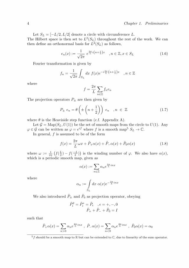
Let SL = [−L/2, L/2] denote a circle with circumference L.The Hilbert space is then set to L2(SL) throughout the rest of the work. We canthen define an orthonormal basis for L2(SL) as follows,
en(x) :=1√2π
e2πL i(n+ 1
2 )x , n ∈ Z, x ∈ SL (1.6)
Fourier transformation is given by
fn =1√2π
∫SL
dx f(x)e−i2πL (n+ 1
2 )x , n ∈ Z
where
f =2π
L
∑n∈Z
fnen
The projection operators P± are then given by
P± en = θ
(±(n+
1
2
))en , n ∈ Z (1.7)
where θ is the Heaviside step function (c.f. Appendix A).Let G = Map(SL, U(1)) be the set of smooth maps from the circle to U(1). Any
ϕ ∈ G can be written as ϕ = eif where f is a smooth map5 SL → C.In general, f is assumed to be of the form
f(x) =2π
Lωx+ P+α(x) + P−α(x) + P0α(x) (1.8)
where ω := 12π
(f(L2 )− f(−L2 )
)is the winding number of ϕ. We also have α(x),
which is a periodic smooth map, given as
α(x) :=∑n∈Z
αne2πL inx
where
αn :=
∫SL
dx α(x)e−2πL inx
We also introduced P± and P0 as projection operator, obeying
P 2ε = P ∗ε = Pε , ε = +,−, 0
P+ + P− + P0 = I
such that
P+α(x) =∑n>0
αne2πL inx , P−α(x) =
∑n<0
αne2πL inx , P0α(x) = α0
5f should be a smooth map to R but can be extended to C, due to linearity of the sum operator.

1.2. Normal ordering 5
For all ϕ ∈ G, we haveΓ(ϕ) = eidΓ(f)
where[dΓ(f1), dΓ(f2)] = iS(f1, f2)
The 2-cocycle becomes
σ(U(f1), U(f2)) = e−iS(f1,f2)/2
by using Eq. (1.32).The choice of phase for the implementer is such that⟨
Γ(eif )⟩
= 0 if ω 6= 0
1.2 Normal ordering
An important mathematical result used for calculations in many-body systems, isthe boson-fermion correspondence (bosonization) in (1 + 1)-dimensions. Normalordering is then required in order to compensate for the infinites that arise fromusing the quasi-free representation. An important aspect of normal-ordering isthat all normal-ordered operator products are well-behaved and have a well-definedoperator product expansion.
1.2.1 Fermion normal-ordering
A fermion normal-ordered operator has a groundstate represented by the vacuumvector Ω, which gives that the vacuum expectation value (VEV) of a fermionnormal-ordered product is always zero. We include the definition of fermion normal-ordering only for bilinear forms of the fermion creation and annihilation operators.
We denote a fermion normal-ordered operator by : : and define the sum operatoras
dΓ(A) ≡ :
∑n,m∈Z
(A)n,m ψ∗nψm
:=∑n,m∈Z
(A)n,m : ψ∗n ψm : (1.9)
where (A)n,m := (en, Aem)H are the matrix element of the operator A. The fermionnormal-ordered form of the bilinear fermion creation and annihilation operators isgiven by
: ψ∗nψm :=
−ψmψ∗n , if n = m < 0
ψ∗nψm , otherwise= ψ∗nψm − θ
(−n− 1
2
)δn,m (1.10)
for all n,m ∈ Z. So in the special case where the operator A is the identity operatorI (where (I)n,m = δn,m), Eq. (1.9) becomes∑
n∈Z: ψ∗nψn : =
∞∑n=0
ψ∗nψn − ψ−n−1ψ∗−n−1 (1.11)

6 Chapter 1. Preliminaries
Equations (1.9) and (1.10), together with
: ψnψm : = ψnψm
: ψ∗nψ∗m : = ψ∗nψ
∗m
for all n,m ∈ Z, define fermion normal-ordering for bilinear forms .
1.2.2 Boson normal-ordering
Boson normal-ordering of operators is denoted by ∗∗∗∗ and is defined by
∗∗R
ωe
∑n∈Z
cnρn∗∗ = ∗∗e
∑n∈Z
cnρnRω∗∗ = e
∑n<0
cnρne
12 c0ρ0Rωe
12 c0ρ0e
∑n>0
cnρn
∗∗AB
∗∗ = ∗∗ (∗∗A
∗∗) (∗∗B
∗∗)∗∗
where ω ∈ Z, A,B are some operators, cn are constants, and the operators R andρn are introduced in Section 1.3. Boson normal-ordering will be used in order toremove divergences from the operators Γ(ϕ), introduced in the previous Section.Note that a boson normal-ordered product of operators is not necessarily a fermionnormal-ordered product, since a boson normal-ordered operator could have a non-zero VEV. Examples of boson normal-ordering are also found in Appendix B andthroughout this work.
1.3 Many-body operators
1.3.1 Operators of interest
Let sn, n ∈ Z, denote the shift operator such that snem = em−n,m ∈ Z. Thematrix elements of the shift operator are given by (sn)n′,m = δn′,m−n, so that themany-body equivalent becomes
ρn := dΓ(sn) =∑m∈Z
: ψ∗m−nψm : (1.12)
The operators ρn, for n 6= 0, are commonly referred to as the oscillation operators,and obey
ρnΩ = 0 ,∀ n ≥ 0 (1.13)
ρ∗n = ρ−n
The oscillation operators obeys the commutation relation
[ρn, ρm] = nδn,−m , ∀n,m ∈ Z (1.14)
Since [sn, sm] = 0, the commutation relation is non-trivial only due to theSchwinger term (see Appendix D.1 for details and proofs). Due to their commuta-tion relation, the oscillation operators can be interpreted as bosonic operators.6
6One can create bosonic operators by rescaling the shift operators by 1/√n, see Eq. (C.2).

1.3. Many-body operators 7
A special case of the oscillation operators is the self-adjoint operator Q definedas
Q := ρ0 = dΓ(I) (1.15)
This operator counts the number of particles minus the number of holes (Q =Nparticles − Nholes) and is equal to the operator in Eq. (1.11). The particles havea positive charge7 1 and the holes have charge −1. So the operator Q representa measurement of the total charge of the system. By definition, the charge of thevacuum is zero. Inserting n = 0 in equation (1.14) gives
[Q, ρm] = 0 ∀ m ∈ Z (1.16)
Thus ρn does not change the total particle number of the system.One other important operator is the ”ladder operators”, defined as
R := Γ(s−1) (1.17)
which, as one can prove, obeys
R−wρnRw = ρn + δn,0 wI , ∀ n,w ∈ Z (1.18)
The unitary operator R raises the total particle number by exactly one, somethingthat no bosonic operator can do due to Eq. (1.16). These operators, commonlyknown as the Klein factors, fills the upper-most empty state of the system, whilethe inverse (Hermitian conjugate) would empty the upper-most filled state.
The precise mathematical construction of the ladder operators are outside thescope of this thesis. For more detail and explicit construction of the Klein factorssee [25]. Due to their properties, the Klein operators are only well defined whenraised to a power which is an integer.
1.3.2 Formal field operators
The fermion field operators are defined as
ψ∗(x) :=1√L
∑n∈Z
ψ∗n e−i 2πL (n+ 1
2 )x , ψ(x) :=1√L
∑n∈Z
ψn ei 2πL (n+ 1
2 )x
in position space, x ∈ SL. They obey the formal CAR.
ψ(x), ψ(y) = ψ∗(x), ψ∗(y) = 0
ψ∗(x), ψ(y) = δ(x− y)
for all x, y ∈ SL and where δ(x) is the Dirac delta-function.
7The charge unit is set to 1 throughout this work

8 Chapter 1. Preliminaries
In position space, the oscillation operator are given by
ρ(x) :=1
L
∑n∈Z
ρnei 2πL nx , x ∈ SL (1.19)
and obey
ρ(x)∗ = ρ(x)
[ρ(x), ρ(y)] =1
2πi∂xδ(x− y) = − 1
2πi∂yδ(x− y) (1.20)
where ∂x := ∂∂x .
By using Eq. (1.12), the operator in Eq. (1.19) can be expressed as
ρ(x) = :ψ∗(x)ψ(x) : (1.21)
and is therefore interpreted as the fermion density operator.
1.3.3 Operator regularization
Note that the formal field operators presented in Section 1.3.2 are operator valueddistributions and should be treated carefully. One way to do that would be to”smear” out the operators with a well defined test-function in order to have a welldefined operator on F .
Another useful method to deal with this problem is to include a regularizationin the Fourier transformation, e.g.
ρε(x) :=∑n∈Z
ρn e2πL inxe−
2πL |n|ε
which is a well defined operator for ε > 0. Taking the limit ε ↓ 0 would then yield theoperator-valued distributions again. This technique simplifies the operator productexpansions (OPE) as it also removes short-distance divergences. This method will,however, only be used in Appendix D.2.
1.4 Formal distributions
In Section 1.3.3 it was made clear that one should be careful when dealing withoperator-valued distributions. But the regularization introduced, while makingthings more well-defined, will complicate some of the calculations in Chapters 3and 4, by adding terms that vanish when taking the limits (ε ↓ 0).
So for this work, the regularization term will be changed from e−ε|n| to e εn,ε > 0. At first, this seems like an ill-advised choice since the sum over positiveintegers, for the real space representation, will grow exponentially. It will not alterthe calculations as all operators and OPE’s will be applied to the vacuum from
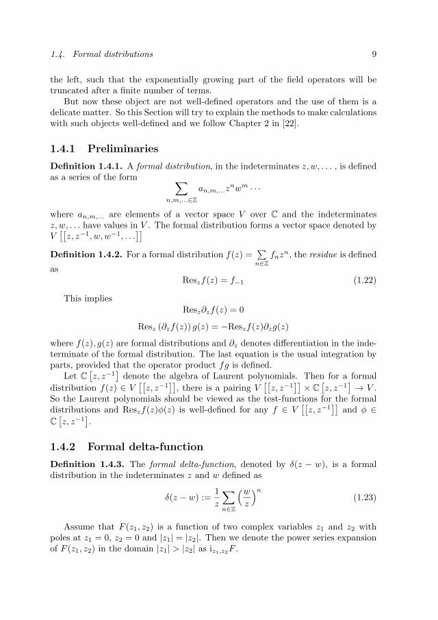
1.4. Formal distributions 9
the left, such that the exponentially growing part of the field operators will betruncated after a finite number of terms.
But now these object are not well-defined operators and the use of them is adelicate matter. So this Section will try to explain the methods to make calculationswith such objects well-defined and we follow Chapter 2 in [22].
1.4.1 Preliminaries
Definition 1.4.1. A formal distribution, in the indeterminates z, w, . . . , is definedas a series of the form ∑
n,m,...∈Zan,m,...z
nwm · · ·
where an,m,... are elements of a vector space V over C and the indeterminatesz, w, . . . have values in V . The formal distribution forms a vector space denoted byV[[z, z−1, w, w−1, . . .
]]Definition 1.4.2. For a formal distribution f(z) =
∑n∈Z
fnzn, the residue is defined
asReszf(z) = f−1 (1.22)
This impliesResz∂zf(z) = 0
Resz (∂zf(z)) g(z) = −Reszf(z)∂zg(z)
where f(z), g(z) are formal distributions and ∂z denotes differentiation in the inde-terminate of the formal distribution. The last equation is the usual integration byparts, provided that the operator product fg is defined.
Let C[z, z−1
]denote the algebra of Laurent polynomials. Then for a formal
distribution f(z) ∈ V[[z, z−1
]], there is a pairing V
[[z, z−1
]]× C
[z, z−1
]→ V .
So the Laurent polynomials should be viewed as the test-functions for the formaldistributions and Reszf(z)φ(z) is well-defined for any f ∈ V
[[z, z−1
]]and φ ∈
C[z, z−1
].
1.4.2 Formal delta-function
Definition 1.4.3. The formal delta-function, denoted by δ(z − w), is a formaldistribution in the indeterminates z and w defined as
δ(z − w) :=1
z
∑n∈Z
(wz
)n(1.23)
Assume that F (z1, z2) is a function of two complex variables z1 and z2 withpoles at z1 = 0, z2 = 0 and |z1| = |z2|. Then we denote the power series expansionof F (z1, z2) in the domain |z1| > |z2| as iz1,z2F .

10 Chapter 1. Preliminaries
The formal delta-function can expanded into different domains as
δ(z − w) = iz,w1
(z − w)− iw,z
1
(z − w)(1.24)
where
iz,w1
z − w=
1
z
∞∑n=0
(wz
)niw,z
1
z − w= −1
z
−∞∑n=−1
(wz
)n
So for all j ∈ N0, we have
∂(j)w δ(z − w) := iz,w
1
(z − w)j+1− iw,z
1
(z − w)j+1
(1.25)
where A(j) := Aj/j! for any operator A.
There are also some important properties of the formal delta-function that areuseful later on.
Proposition 1.4.4. 1. For any formal distribution f(z) ∈ V[[z, z−1
]]Reszf(z)δ(z − w) = f(w) (1.26)
and the product f(z)δ(z − w) is well-defined.
2.
f(z)δ(z − w) = f(w)δ(z − w) (1.27)
3.
δ(z − w) = δ(w − z) (1.28)
4. For all j ∈ N0
∂(j)z δ(z − w) = (−1)j∂(j)
w δ(z − w) (1.29)
Proof. See Appendix E.1.1

1.5. Baker-Campbell-Hausdorff formulas 11
We define the formal sign function as
sign(z − w) := − iπ
ln
(z
|z|
)− ln
(w
|w|
)+
∑n∈Z\0
1
n
( zw
)n (1.30)
which satisfies
sign(z − w) = −sign(w − z)2πi
Lz∂zsign(z − w) =
2z
Lδ(z − w)
For indeterminates z ∝ ei 2πL y and w ∝ ei 2πL x, x, y ∈ SL, of a formal distribution,the integral over the variable y can be changed to∫
SL
dy
L(·) =
∮γ
dz
2πi
1
z(·) = Resz
1
z(·)
So the formal distribution zLδ(z −w) is the equivalence of the Dirac delta function
on the circle SL since8
∫SL
dy
Lzδ(z − w) =
∮γ
dz
2πi
1
zzδ(z − w) = Reszδ(z − w) =
∫SL
dy δ(y − x)
Most of the calculations done using formal distributions where checked by usingthe regularized operators (c.f. Section 1.3.3). There were no relevant deviation.Interested readers are encouraged to check for themselves.
1.5 Baker-Campbell-Hausdorff formulas
For the convenience of the reader, we collect various Baker-Campbell-Hausdorff(BCH) type formulas that will be used repeatedly.
Let A and B be two arbitrary operators and h(A) some function of A.
Lemma 1.5.1. For C := [A,B] satisfying [A,C] = [B,C] = 0, the following holds
1.
e−BAeB = A+ C
which gives that [A, eB
]= C eB (1.31)
8There is an abuse of notation as both the formal delta function and the Dirac delta aresymbolized by a δ.

12 Chapter 1. Preliminaries
2.e−Bh(A)eB = h(A+ C) (1.32)
3.eAeB = eC/2eA+B = eCeBeA (1.33)
Proof. See Appendix E.1.2
Lemma 1.5.2. For any operators A and B satisfying [A,B] = CB and [A,C] =[B,C] = 0, then h(A)B = Bh(A+ C).
Proof. Taylor expanding h(A) and using that AnB = B(A + C)n since AB =B(A+ C).
The special case of h(A) = eA is an important relation for this work, and gives
eAB = BeA+C
BeA = eA−CB (1.34)

Chapter 2
Anyons in (1 + 1) dimensions
Abelian anyons are defined by their exchange relation where they obtain any phaseshift.
Abelian anyon quantum field operators should therefore satisfy the relation
φ1(x)φ2(y) = eiϑsgn(x−y)φ2(y)φ1(x) , x 6= y, x, y ∈ SL, and ϑ ∈ R (2.1)
where ”sgn” is the sign function. It is clear from the relation above that, if ϑ is aneven multiplet of π, the anyons become bosons, while if ϑ is an odd integer times π,the anyons exhibit fermionic properties. As mentioned in the introduction, there isa interesting relation between anyons and the FQHE which serves as a motivationfor this work.
This Chapter will give a brief introduction to the boson-fermion correspondencein (1 + 1) dimensions and the extension which allow us to construct (1 + 1) dimen-sional1 anyon field operators. Then continue by introducing the corresponding dualanyon field operator and show some very interesting properties.
2.1 Boson-fermion correspondence
In (1 + 1) dimensions, there exist relations between fermions and bosons. One ofthese relations was given by Eq. (1.21). Another is the following.
1Normally when talking about anyons, they are referring to the quasi-particles in (2 + 1)dimensions. We therefore stress that the anyon operators that we are using are in (1+1) dimensionsonly.
13

14 Chapter 2. Anyons in (1 + 1) dimensions
Lemma 2.1.1. All vectors in the fermion Fock space F can be represented as linearcombinations of
B(mn∞n=1 , ω) =
∞∏n=1
1√mn!
(ρ−n√n
)mnRωΩ ,mn ∈ N0, ω ∈ Z,
∑n
mn <∞
(2.2)or of
F (mk, nk∞k=0) =
∞∏k=0
(ψ∗k)mk (ψ−k−1)
nkΩ ,mk, nk ∈ 0, 1 ,∑k
mk + nk <∞
(2.3)Both form a complete orthonormal basis that can be used to span the entire Fockspace.
Proof. See Appendix C.1.
Lemma 2.1.1 allows every operator in the fermion Fock space F to be expressedin terms of the Klein factors and oscillation operators.
The indeterminates of the formal distributions, w and z, that are used through-out this work are defined as
w := e2πL ixe
2πL ε (2.4)
z := e2πL iye
2πL ε′
(2.5)
where x, y ∈ SL and ε, ε′ are constants greater than zero.
Proposition 2.1.2. The fermion operators can be written as
ψ(z) :=1√LeiπLyQR−1ei
πLyQe
∑n<0
1nρnz
n
e
∑n>0
1nρnz
n
ψ∗(z) :=1√Le−i
πLyQRe−i
πLyQe
−∑n<0
1nρnz
n
e−∑n>0
1nρnz
n
(2.6)
Proof. See Appendix E.2.1
The normalization factor 1√L
ensures that the operators obey the formal CAR
and that they have the correct dimensions.Introducing the regularized map from the circle to the real axis fz(s−1) ∈
Map(SL,C), where s−1 is the shift operator for n = −1, as
fz(s−1) := −i ln
(s−1
|s−1|
)+ i ln
(z
|z|
)+ α−z (s−1) + α+
z (s−1) (2.7)
where α± ∈ C∞(SL,C) is a smooth map from the circle onto the complex plane,defined as
α±z (s−1) := ±i∞∑n=1
1
n
(z±n
)s±n (2.8)
such that P±ρ(z) = − iLz∂zdΓ(α±z ), for ρ(z) := 1
L
∑n∈Z
ρnzn.

2.2. Boson-anyon correspondence 15
It is proven in [19] that the maps fz and α±z obey
1) iS(α+z , α
−w) = iα−z (w) (2.9)
2) iS(fz, fw) = −iS(fw, fz) = ifw(z) (2.10)
Proposition 2.1.2 and Eqs. (2.7)-(2.10) and gives
ψ(z) =1√L∗∗Γ(e−ifz )∗∗
ψ∗(z) =1√L∗∗Γ(eifz )∗∗
ψ∗(w)ψ(z) = e−iπ sign(w−z)ψ(z)ψ∗(w) , w 6= z (2.11)
where the sign function is given by
sign(w − z) =1
πfz(w) (2.12)
Using equation (2.11) yields2 the formal CAR. For greater details, see [26] or [27].
2.2 Boson-anyon correspondence
The unitary operators ∗∗Γ(eif )∗∗ can be extended as ∗∗Γ(eif )∗∗ → ∗∗Γ(eimf )∗∗. These
operators are commonly known as vertex operators and obey the exchange relation
∗∗Γ(eim1fw)∗∗
∗∗Γ(eim2fz )∗∗ = eiπm1m2 sign(w−z) ∗
∗Γ(eim2fz )∗∗∗∗Γ(eim1fw)∗∗
which is fermionic if m1m2 is an odd integer and bosonic if m1m2 is even. Thetransformation is only well-defined iff m1,m2 ∈ Z, due to the restrictions fromthe Klein factors on the vertex operators. This does not meet the requirement forabelian anyons, where m1m2 should be any real number.
It can be shown that the 2-cocycle of Eq. (1.8) is invariant under rescalingsuch3 as ω → ω
λ , P0α(x) → λP0α(x) for all λ 6= 0 [19]. We introduce the rescaling
parameter ν0(∈ R \ 0) and transform f such that
fz(s−1)→ fz(s−1) := − i
ν0ln (s−1) + iν0 ln
(z
|z|
)+ α+
z (s−1) + α−z (s−1) (2.13)
obeying
iS(fw, fz) = iS(fw, fz) = iπ sign(w − z)2It is actually the vacuum expectation value, of the anti-commutation, that yields the CAR3ω is the winding number (c.f. Eq. (1.8)) and not to be confused with an indeterminate of a
formal distribution
16 Chapter 2. Anyons in (1 + 1) dimensions
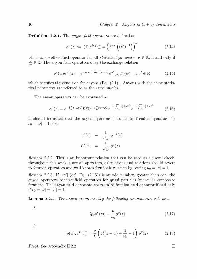
Definition 2.2.1. The anyon field operators are defined as
φν(z) := ∗∗Γ(eiνfz )∗∗ =
(φ−ν
((z∗)
−1))∗
(2.14)
which is a well-defined operator for all statistical parameter ν ∈ R, if and only ifνν0∈ Z. The anyon field operators obey the exchange relation
φν(w)φν′(z) = e−iπνν
′ sign(w−z)φν′(z)φν(w) , νν′ ∈ R (2.15)
which satisfies the condition for anyons (Eq. (2.1)). Anyons with the same statis-tical parameter are referred to as the same species.
The anyon operators can be expressed as
φν(z) = e−iπLνν0yQR
νν0 e−i
πLνν0yQe
−ν∑n<0
1nρnz
n
e−ν
∑n>0
1nρnz
n
(2.16)
It should be noted that the anyon operators become the fermion operators forν0 = |ν| = 1, i.e.
ψ(z) =1√Lφ−1(z)
ψ∗(z) =1√Lφ1(z)
Remark 2.2.2. This is an important relation that can be used as a useful check,throughout this work, since all operators, calculations and relations should revertto fermion operators and well known fermionic relation by setting ν0 = |ν| = 1.
Remark 2.2.3. If |νν′| (c.f. Eq. (2.15)) is an odd number, greater than one, theanyon operators become field operators for quasi particles known as compositefermions. The anyon field operators are rescaled fermion field operator if and onlyif ν0 = |ν| = |ν′| = 1.
Lemma 2.2.4. The anyon operators obey the following commutation relations
1.
[Q,φν(z)] =ν
ν0φν(z) (2.17)
2.
[ρ(w), φν(z)] =ν
L
(zδ(z − w) +
1
ν0− 1
)φν(z) (2.18)
Proof. See Appendix E.2.2

2.3. Dual anyon operators 17
2.3 Dual anyon operators
The result collected in the previous Section are well known (c.f. [19]). This Sectionwill introduce the corresponding dual anyon field operator and its relation to theanyon field operators.
Postulate 2.3.1. The operators φ−1ν , ν ∈ R \ 0, correspond to the dual anyon
field operator of species ν and is defined as
φ−1ν (z) := ∗
∗Γ(e−iν fz )∗∗ = ei
πLν0ν yQR−
1νν0 ei
πLν0ν yQe
1ν
∑n<0
1nρnz
n
e1ν
∑n>0
1nρnz
n
(2.19)
and is a well-defined operator iff 1νν0∈ Z. The dual anyon field operators satisfy
the exchange relation for abelian anyon operators, with a phase shift of ϑ = πνν′ ∈ R
(c.f. Eq. (2.1)).
It is later shown that there is a natural extension between the anyon secondorder differential operator of species ν and −1/ν (c.f. Section 3.2.2) and thatvectors created by using anyon and dual anyon operators are eigenvectors of theseoperators with different eigenvalues (c.f. Section 4.1).
Proposition 2.3.2. The anyon and dual anyon operators obey the CARφν(w), φ−
1ν (z)
= zδ(z − w) ∗∗φ
ν(w)φ−1ν (z)∗∗ (2.20)
for all ν.
Proof. See Appendix E.2.3
This is very similar to the anti-commutation relation that the bosonized fermionfield operators obey.
Remark 2.3.3. Proposition 1.4.4 2 yields
δ(z − w)∗∗φν(w)φ−
1ν (z)∗∗ = δ(z − w)∗∗φ
ν(z)φ−1ν (z)∗∗ = δ(z − w)φ(ν− 1
ν )(z) (2.21)
which gives φν(w), φ−
1ν (z)
= zδ(z − w)φ(ν− 1
ν )(z) (2.22)
It is natural to prescribe the conjugate of the anyon field operators (φ−ν) as thecorresponding dual anyon operators. This prescription does not satisfy the relationfor a dual particle. Comparing Eq. (2.20) with the relation between the anyonoperator and its conjugate, which obeys a non-canonical commutation relations for
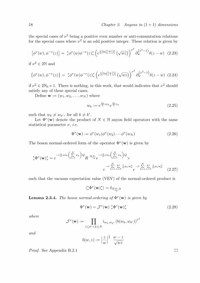
18 Chapter 2. Anyons in (1 + 1) dimensions
the special cases of ν2 being a positive even number or anti-commutation relationsfor the special cases where ν2 is an odd positive integer. These relation is given by
[φν(w), φ−ν(z)
]= ∗∗φν(w)φ−ν(z)∗∗
(e
12 |ln(|wz |)| (√wz))ν2
∂(ν2−1)w δ(z − w) (2.23)
if ν2 ∈ 2N and
φν(w), φ−ν(z)
= ∗∗φν(w)φ−ν(z)∗∗
(e
12 |ln(|wz |)| (√wz))ν2
∂(ν2−1)w δ(z − w) (2.24)
if ν2 ∈ 2N0 + 1. There is nothing, in this work, that would indicates that ν2 shouldsatisfy any of these special cases.
Define w := (w1, w2, . . . , wN ) where
wk := e2πL ixke
2πL εk (2.25)
such that wk 6= wk′ , for all k 6= k′.Let Φν(w) denote the product of N ∈ N anyon field operators with the same
statistical parameter ν, i.e.
Φν(w) := φν(w1)φν(w2) · · ·φν(wN ) (2.26)
The boson normal-ordered form of the operator Φν(w) is given by
∗∗Φ
ν(w)∗∗ = e−i πLνν0
(N∑k=1
xk
)QR N ν
ν0 e−i πLνν0
(N∑k=1
xk
)Q×
e−ν
N∑k=1
∑n<0
1nρnw
nk
e−ν
N∑k=1
∑n>0
1nρnw
nk
(2.27)
such that the vacuum expectation value (VEV) of the normal-ordered product is
〈∗∗Φν(w)∗∗〉 = δN νν0,0
Lemma 2.3.4. The boson normal-ordering of Φν(w) is given by
Φν(w) = J ν(w) ∗∗Φν(w)∗∗ (2.28)
whereJ ν(w) :=
∏1≤k′<k≤N
iwk,wk′ (b(wk, wk′))ν2
and
b(w, z) :=∣∣∣ zw
∣∣∣ 12 w − z√wz
Proof. See Appendix B.2.1

2.3. Dual anyon operators 19
Let Φ(wk, νkNk=1) denote the product of N (∈ N) anyon field operators of dif-ferent species, i.e.
Φ(wk, νkNk=1) := φν1(w1)φν2(w2) · · ·φνN (wN )
where νkν0∈ Z ∀k and wk 6= wk′ for all k 6= k′. The boson normal-ordered form of
the operator Φ(wk, νkNk=1) is given by
∗∗Φ(wk, νkNk=1)∗∗ = e
−i πLν0(N∑k=1
νkxk
)QR
1ν0
N∑k=1
νke−i πLν0
(N∑k=1
νkxk
)Q×
e−
N∑k=1
∑n<0
νkn ρnw
nk
e−
N∑k=1
∑n>0
νkn ρnw
nk
such that the VEV becomes⟨∗∗Φ(wk, νkNk=1)∗∗
⟩= δ
1ν0
N∑k=1
νk,0
Lemma 2.3.5. Boson normal-ordering the operator Φ(wk, νkNk=1) gives
Φ(wk, νkNk=1) = I(wk, νkNk=1) ∗∗Φ(wk, νkNk=1)∗∗ (2.29)
whereI(wk, νkNk=1) :=
∏1≤k<k′≤N
iwk′ ,wk (b(wk′ , wk))νkνk′
and b(wk′ , wk) is defined in Lemma 2.3.4.
Proof. See Appendix B.2.2
Define z := (z1, z2, . . . , zM ) where
zj := e2πL iyje
2πL ε′j (2.30)
such that zj 6= zj′ for all j 6= j′ and zj 6= wk ∀j, k.Let ϕν(z,w) denote the product of M ∈ N dual anyon operators and N ∈ N
anyon operators, i.e.ϕν(z,w) := Φ−
1ν (z)Φν(w) (2.31)
where Φν(w) is the same as in Eq. (2.26). The boson normal-ordered form of theoperator ϕν(z,w) is given by
∗∗ϕ
ν(z,w)∗∗ =
e−i πLν0
(νN∑k=1
xk− 1ν
M∑j=1
yj
)Q
RNνν0−M 1
νν0 e−i πLν0
(νN∑k=1
xk− 1ν
M∑j=1
yj
)Q
× e−∑n<0
1nρn
(νN∑k=1
wnk− 1ν
M∑j=1
znj
)e−∑n>0
1nρn
(νN∑k=1
wnk− 1ν
M∑j=1
znj
)
such that the VEV is〈∗∗ϕν(z,w)∗∗〉 = δN ν
ν0−M 1
νν0,0

20 Chapter 2. Anyons in (1 + 1) dimensions
Lemma 2.3.6. Boson normal-ordering the operator ϕν(z,w) yields
ϕν(z,w) = J− 1ν (z)J ν(w)
M∏j=1
N∏k=1
iwk,zj1
b(wk, zj)∗∗ϕ
ν(z,w)∗∗ (2.32)
Proof. This comes from boson normal-ordering the two different operators Φν(w)
and Φ−1ν (z) separately by using Lemma 2.3.4. Then use Lemma 2.3.5 for the special
case of two boson normal-ordered operators.
Remark 2.3.7. If the operator product was instead given byϕν(z,w) := Φν(w)Φ−
1ν (z) the boson normal-ordering of the field operator would
be given by
ϕν(z,w) = J− 1ν (z)J ν(w)
N∏k=1
M∏j=1
izj ,wk1
b(zj , wk)∗∗ϕ
ν(z,w)∗∗
where ∗∗ϕν(z,w)∗∗ = ∗∗ϕ
ν(z,w)∗∗.

Chapter 3
Anyons and the CS model
The first part of this Chapter will give a short description of the integrable Calogero-Sutherland (CS) models expressed in terms of the indeterminates of formal distri-butions. We will then show that the Laughlin wavefunction reduces to the CSgroundstate, up to a constant factor and with a center of mass (CoM) shift, whenrestricted to the boundaries of a circular quantum Hall droplet. We will also givea brief introduction to a generalization of the CS model which is referred to as thedeformed Calogero-Sutherland (dCS) model [4] [5].
In the second part of this Chapter we will introduce a self-adjoint operator Hν,3by generalizing the construction of the fermion W -algebra for anyon field operators.This operator Hν,3 was previously constructed in [19] using a somewhat differentmethod. We will also show some interesting relations of the Hν,3 operator.
In the final Section we show that the expectation value of the Hν,3 operator andthe product of N ∈ N anyon field operators yields the CS groundstate, with a CoMshift, and the CS Hamiltonian.
3.1 The Calogero-Sutherland type model
The CS model describes an N -body system on a circle of length L interacting witha translationally invariant centrifugal (inverse quadratic) potential. The model wasfirst proposed by F. Calogero in [2] which also included a harmonic (quadratic)potential and fully solved for the three-body case in [28] and for arbitrary N in [1].The model was extended to translationally invariant systems by B. Sutherlandin [3], and solved fully in [29]. The CS model was originally expressed in terms ofvariables on the circle SL, we find it convenient to re-express them in this Sectionin terms of the indeterminates of a formal distribution, wk and zj (c.f. Eqs. (2.25)and (2.30)).
21

22 Chapter 3. Anyons and the CS model
3.1.1 The CS model
The Calogero-Sutherland model is a quantum many-body model of N(∈ N) indis-tinguishable particles interacting via a translationally invariant two-body potential.The model has the groundstate (GS) wavefunction
ψ0(w) =∏k′<k
(1
2i
wk − wk′√wkwk′
)λ(3.1)
where w = (w1, . . . , wN ) such that wk 6= wk′ for all k 6= k′. The GS wavefunctioncorresponds to the CS Hamiltonian defined as
HN :=4π2
L2
N∑k=1
(wk∂wk)2
+ g4π2
L2
∑k′<k
V (wk, wk′) (3.2)
with the two-body potential
V (wk, wk′) := − wkwk′
(wk − wk′)2 (3.3)
and the coupling constant g = 2λ (λ− 1), with the constraint g > − 14 in order to
avoid an energy spectrum that is unbounded from below. The GS wavefunctioncorresponds to an eigenvalue of
E0 =π2λ2N
(N2 − 1
)3L2
(3.4)
The CS Hamiltonian has exact eigenfunctions of the form
Ψn(w) = Pn,λ(w)ψ0(w) (3.5)
with n = (n1, n2, . . . , nN ) ∈ NN , and Pn,λ(w) are symmetric1 polynomials.The model describes fermions for λ an odd integer and hard sphere bosons when
λ is an even integer. The special case of λ = 1 would give a model describing Nfree fermions on a circle with periodic boundary conditions.
When λ is any real number, the GS wavefunction gains a phase shift of e±iπλ
during particle position exchange.
3.1.2 Relation to the Laughlin state
The Laughlin state [9] is given by2
Ψ(m; z1, . . . , zN ) = e−
N∑l=1
|zl|2 ∏l<l′
(zl′ − zl)2m+1
, m ∈ N0 (3.6)
1w.r.t. particle position permutation2The magnetic length lB is set to 1

3.1. The Calogero-Sutherland type model 23
where3 2m + 1 corresponds to one over the filling factor and zl := 12 (Xl + iYl)
is a dimensionless complex number representing the position of the l-th electron,(Xl, Yl), in the 2-dimensional quantum Hall (QH) droplet.
The low energy degrees of freedom of a QH liquid are at the boundary, due tothe incompressibility of the QH liquid. For electrons at the edge of a circular QHdroplet with radius r we have
zl =1
2reiϑl , ϑl ∈ S2π
Inserting this ansatz into the Laughlin state yields
Ψ(m;ϑ1, . . . , ϑN ) = e− 1
4 r2N∑l=1
1 ∏l<l′
(r2
)2m+1 (eiϑl′ − eiϑl
)2m+1
= (ir)N(2m+1)N−1
2 e−14 r
2N∏l<l′
ei(2m+1)ϑl′+ϑl
2
(sin
(ϑl′ − ϑl
2
))2m+1
(3.7)
Comparing Eqs. (3.7) and (3.1) (or rather Eq. (2)) shows that the Laughlinwavefunction for the electrons at the edge of the QH droplet corresponds to theCS groundstate, up to a constant4 and a CoM shift, for L = 2π and λ = 2m + 1.This suggests that the CS groundstate wavefunction describes the edge degrees offreedom of a QH liquid.
3.1.3 The deformed Calogero-Sutherland model
The deformed Calogero-Sutherland (dCS) model is defined by the differential op-erator
HN,M :=4π2
L2
N∑k=1
(wk∂wk )2 − 4π2
L2λ
M∑j=1
(zj∂zj
)2+
4π2
L22 (λ− 1)
1
λ
∑j′<j
V (zj , zj′) + λ∑k′<k
V (wk, wk′)
+
4π2
L22 (1− λ)
M∑j=1
N∑k=1
V (wk, zj) (3.8)
where the two-body potential is given by Eq. (3.3).
3Note that the zl used in Laughlin’s wavefunction are not indeterminates of formal distribu-tions.
4Note that none of the wavefunction have been normalized

24 Chapter 3. Anyons and the CS model
The dCS model has exact eigenfunctions similar to Eq. (3.5), with ψ0 replacedby ψ0(z,w) , which we refer to as the deformed groundstate (dGS) eigenfunction,defined as
ψ0(z,w) :=∏j′<j
(1
2i
zj − zj′√zjzj′
)λ−1 ∏k′<k
(1
2i
wk − wk′√wkwk′
)λ M∏j=1
N∏k=1
(1
2i
wk − zj√wkzj
)−1
(3.9)which corresponds to an eigenvalue
E0 :=π2
3L2
(Nλ−M) (Nλ− λ−M) (Nλ+ λ−M)−M(λ2 − 1
)λ
(3.10)
of the dCS differential operator.
Remark 3.1.1. Due to the sign in front of the z-derivatives, the differential operatorsHN,M cannot represent a physical system for λ > 0 and the dGS eigenfunction isnot square integrable. So the dCS model, unlike the original CS model, cannot beconsidered as a quantum mechanical model.
3.2 The Hν,s operators
As shown in Appendix D.1, there exists fermion operators such that
[W s, ψ(∗)(w)
]=
(2π
L
)s−1
(w∂w)s−1
ψ(∗)(w)
which can also be expressed in terms of the fermion density operators (c.f. AppendixD.2)
Since the anyon field operators are a generalization of the fermion field operatorsthere should exist a generalization of the fermion W s operators. It turns out thatthis is not as simple since there arises a need for correction terms for higher orderderivatives. We construct the generalization of the W s operators for s = 1, 2, 3,which was introduced in [19], using a different method.
3.2.1 Construction of the anyon differential operators
It is not trivial to construct the second quantization of the anyon differential oper-ators. The first additional terms manifests for the second derivative (c.f. AppendixD.3.2). We restrict ourselves to the s ≤ 3 operators (higher order derivatives areinteresting but outside the scope of this thesis).
There exists a generalization of the fermion W s operators for anyons with sta-tistical parameter ν and is denoted by W ν,s.

3.2. The Hν,s operators 25
Lemma 3.2.1. The W ν,s operators, for s = 1, 2, obey
[W ν,s, φν(w)] = ν2−s(
2π
L
)s−1
(w∂w)s−1
φν(w) s = 1, 2 (3.11)
For s > 2 operators additional terms arise.
Proof. see Appendix D.3.2
For the first two cases, s = 1, 2, it is a minor challenge to construct the desiredoperators for the anyon field operators.
Lemma 3.2.2. The Hν,s, s = 1, 2, operators are defined as
Hν,s :=1
ν2−sWν,s (3.12)
and obey
Hν,sΩ = 0 (3.13)
[Hν,s, φν(w)] =
(2π
Lw∂w
)s−1
φν(w) (3.14)
for all ν.
Proof. This can be seen from Eq. (3.11) in Lemma 3.2.3 and Section D.3.
It is natural to interpret the Hν,1 operator as the charge operator for anyonswith statistical parameter ν. Equations (3.11) and (D.26) gives that the first orderdifferential operator is not actually dependent on the statistical parameter ν (onlyν0), but is will still be written as Hν,2 in order to have a unified notation.
The operator of interest is for s = 3.
Lemma 3.2.3. The W ν,3 operator and the anyon field operator obey
[W ν,3, φν(w)
]=
1
ν
4π2
L2(w∂w)
2φν(w)
− 4π2
L
(ν2 − 1
) ∗∗ (w∂wρ(w))φν(w)∗∗ +
π2(ν2 − 1
) (ν2 − 2
)3νL2
φν(w) (3.15)
Proof. see Appendix D.3.2
There are two terms that need to be eliminated. This is partially done by theintroduction of the C operator.
26 Chapter 3. Anyons and the CS model
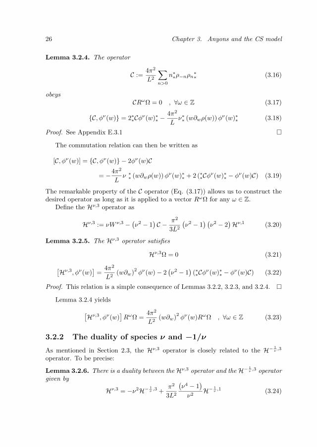
Lemma 3.2.4. The operator
C :=4π2
L2
∑n>0
n∗∗ρ−nρn∗∗ (3.16)
obeysCRωΩ = 0 , ∀ω ∈ Z (3.17)
C, φν(w) = 2∗∗Cφν(w)∗∗ −4π2
Lν∗∗ (w∂wρ(w))φν(w)∗∗ (3.18)
Proof. See Appendix E.3.1
The commutation relation can then be written as
[C, φν(w)] = C, φν(w) − 2φν(w)C
= −4π2
Lν ∗∗ (w∂wρ(w))φν(w)∗∗ + 2 (∗∗Cφν(w)∗∗ − φν(w)C) (3.19)
The remarkable property of the C operator (Eq. (3.17)) allows us to construct thedesired operator as long as it is applied to a vector RωΩ for any ω ∈ Z.
Define the Hν,3 operator as
Hν,3 := νW ν,3 −(ν2 − 1
)C − π2
3L2
(ν2 − 1
) (ν2 − 2
)Hν,1 (3.20)
Lemma 3.2.5. The Hν,3 operator satisfies
Hν,3Ω = 0 (3.21)
[Hν,3, φν(w)
]=
4π2
L2(w∂w)
2φν(w)− 2
(ν2 − 1
)(∗∗Cφν(w)∗∗ − φν(w)C) (3.22)
Proof. This relation is a simple consequence of Lemmas 3.2.2, 3.2.3, and 3.2.4.
Lemma 3.2.4 yields[Hν,3, φν(w)
]RωΩ =
4π2
L2(w∂w)
2φν(w)RωΩ , ∀ω ∈ Z (3.23)
3.2.2 The duality of species ν and −1/ν
As mentioned in Section 2.3, the Hν,3 operator is closely related to the H− 1ν ,3
operator. To be precise:
Lemma 3.2.6. There is a duality between the Hν,3 operator and the H− 1ν ,3 operator
given by
Hν,3 = −ν2H− 1ν ,3 +
π2
3L2
(ν4 − 1
)ν2
H− 1ν ,1 (3.24)
3.2. The Hν,s operators 27
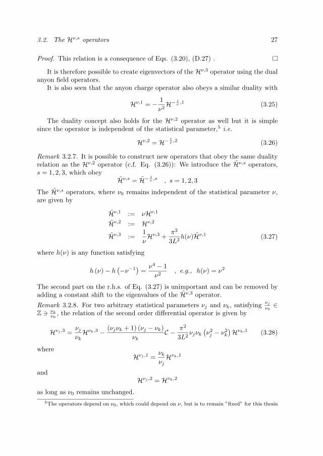
Proof. This relation is a consequence of Eqs. (3.20), (D.27) .
It is therefore possible to create eigenvectors of the Hν,3 operator using the dualanyon field operators.
It is also seen that the anyon charge operator also obeys a similar duality with
Hν,1 = − 1
ν2H− 1
ν ,1 (3.25)
The duality concept also holds for the Hν,2 operator as well but it is simplesince the operator is independent of the statistical parameter,5 i.e.
Hν,2 = H− 1ν ,2 (3.26)
Remark 3.2.7. It is possible to construct new operators that obey the same dualityrelation as the Hν,2 operator (c.f. Eq. (3.26)): We introduce the Hν,s operators,s = 1, 2, 3, which obey
Hν,s = H− 1ν ,s , s = 1, 2, 3
The Hν,s operators, where ν0 remains independent of the statistical parameter ν,are given by
Hν,1 := νHν,1
Hν,2 := Hν,2
Hν,3 :=1
νHν,3 +
π2
3L2h(ν)Hν,1 (3.27)
where h(ν) is any function satisfying
h (ν)− h(−ν−1
)=ν4 − 1
ν2, e.g., h(ν) = ν2
The second part on the r.h.s. of Eq. (3.27) is unimportant and can be removed byadding a constant shift to the eigenvalues of the Hν,3 operator.
Remark 3.2.8. For two arbitrary statistical parameters νj and νk, satisfyingνjν0∈
Z 3 νkν0
, the relation of the second order differential operator is given by
Hνj ,3 =νjνkHνk,3 − (νjνk + 1) (νj − νk)
νkC − π2
3L2νjνk
(ν2j − ν2
k
)Hνk,1 (3.28)
whereHνj ,1 =
νkνjHνk,1
andHνj ,2 = Hνk,2
as long as ν0 remains unchanged.
5The operators depend on ν0, which could depend on ν, but is to remain ”fixed” for this thesis

28 Chapter 3. Anyons and the CS model
Remark 3.2.9. The Hν,3 operator in Eq. (3.27) with h(ν) = ν2 has an interestingrelation for two arbitrary statistical parameters νj , νk, defined as in Remark 3.2.8,given by
Hνj ,3 = Hνk,3 +(νkνj + 1) (νk − νj)
νjνkC
3.2.3 The groundstate eigenvector
It is later shown that there exists certain eigenvectors of the Hν,3 operator that areof particular interest for the CS or dCS models (c.f. Corollary 3.3.5 or Theorem4.2.1). The construction and implementation of all of these eigenvectors is outsidethe scope of this thesis, and we restrict ourselves to only the simplest eigenvectors.
Lemma 3.2.10. The vector
η0 := RωHΩ , ωH ∈ Z (3.29)
is an eigenvector of the Hν,3 operator and corresponds to an eigenvalue of Hν,3,
Hν,3η0 = E0η0 , E0 :=π2
3L2
(4νν3
0ω3H − ν3ν0ωH
)(3.30)
Proof. Using Eqs. (3.20) and (3.17) gives that the C operator vanishes when appliedto a vector such as η0 for all ωH ∈ Z. Using Eq. (D.27) for the W ν,3 operator andthe fact that the W s commute with the Klein factors and annihilate the vacuumimplies that only the charge operator remain. Thus, Eq. (3.30) can be rewritten as
Hν,3η0 = ν
(4π2ν3
0
3L2Q3 +
π2ν0
(2− 3ν2
)3L2ν2
Q
)η0 +
π2ν0
3L2ν
(ν2 − 1
) (ν2 − 2
)Qη0
whereQη0 = ωHη0
which gives Eq. (3.30).
The parameter ωH is determined such that
〈η0,Ψ〉 6= 0 (3.31)
where Ψ ∈ F is an eigenvector of the Hν,3 operator. The relation given by Eq.(3.31) will be seen in Sections 3.3 and 4.1 where Ψ will correspond to an vectorcreated by using the anyon and dual anyon field operators.
The two cases that are of interest for this thesis are the vectors ηCS and ηdCS
defined as
ηCS := R
(N νν0
)Ω , N ∈ N (3.32)
ηdCS := R
(N νν0−M 1
νν0
)Ω , N,M ∈ N (3.33)
where ηCS and ηdCS corresponds to the CS and dCS model respectively. We referto these eigenvectors as the groundstate eigenvectors and the reason will becomeclear in Corollary 3.3.6 and Corollary 4.2.2.

3.3. Anyons relation to the CS model 29
See [19] for the construction of an η eigenvector corresponding to the exacteigenfunctions of the CS model.
Using Eq. (3.32) for the groundstate eigenvalue in Eq. (3.30) does not givethe exact groundstate eigenvalue of the CS model (c.f. Eq. (3.4)). This is due toa CoM shift that arises from using the groundstate vectors as will be seen moreclearly in Sections 3.3 and 4.2.
3.3 Anyons relation to the CS model
Definition 3.3.1. Let A and B be two arbitrary operators where B = N ∗∗B∗∗. The∗ - operation is defined as
A ∗B := N ∗∗AB∗∗For this Section, we define Φν(w) as the product of N anyon operator with the
same statistical parameter ν, i.e.
Φν(w) := φν(w1) · · ·φν(wN )
with w = (w1, . . . , wN ) where wk 6= wk′ for all k 6= k′ and such that 1 < |w1| <|w2| < . . . < |wN | <∞
Lemma 3.3.2. The operators Φν(w) and W ν,3 obey the commutation relation
ν[W ν,3,Φν(w)
]=
4π2
L2
N∑k=1
(wk∂wk)2
Φν(w)
− 4π2
Lν(ν2 − 1
) N∑k=1
(wk∂wkρ(wk)) ∗ Φν(w)
− 4π2
L22ν2
(ν2 − 1
) ∑k′<k
wkwk′
(wk − wk′)2 Φν(w)
+π2
3L2
(ν2 − 1
) (ν2 − 2
)NΦν(w) (3.34)
This relation hold for all ν.
Proof. See Appendix E.3.2
Lemma 3.3.3. The C operator, defined in Lemma 3.2.4, and the operator Φν(w)obey the anti-commutation relation
C,Φν(w) = 2C ∗ Φν(w)− 4π2
L2ν
N∑k=1
(wk∂wkρ(wk)) ∗ Φν(w) (3.35)
Proof. See Appendix E.3.3

30 Chapter 3. Anyons and the CS model
Proposition 3.3.4. The Hν,3 operator and the N -body anyon operator Φν(w) obeythe commutation relation
[Hν,3,Φν(w)
]=
4π2
L2
N∑k=1
(wk∂wk)2
Φν(w)
− 4π2
L22ν2
(ν2 − 1
) ∑k′<k
wkwk′
(wk − wk′)2 Φν(w)
− 2(ν2 − 1
)(C ∗ Φν(w)− Φν(w)C) (3.36)
Proof. This can be obtained by using Lemmas 3.3.2 and 3.3.3 and that[Hν,1,Φν(w)
]= NΦν(w).
The last two terms in Eq. (3.36) vanish if applied to a vector RωΩ, ω ∈ Z, dueto the property of the C operator (c.f. Lemma 3.2.4), i.e.
[Hν,3,Φν(w)
]RωΩ =
4π2
L2
N∑k=1
(wk∂wk)2
Φν(w)RωΩ
− 4π2
L22ν2
(ν2 − 1
) ∑k′<k
wkwk′
(wk − wk′)2 Φν(w)RωΩ (3.37)
Comparing Eqs. (3.2) and (3.37) gives that[Hν,3,Φν(w)
]RωΩ = HNΦν(w)RωΩ
where HN is the CS Hamiltonian with coupling constant g = 2ν2(ν2 − 1
).
Corollary 3.3.5. Let η be an eigenvector of the Hν,3 operator belonging to a dense,invariant domain and satisfying
Hν,3η = Eη
Then the following function
Fη(w) := 〈η,Φν(w)Ω〉
is an eigenfunction of the CS Hamiltonian, given in Eq. (3.2) for λ = ν2, witheigenvalue E.
Proof. This is a simple consequence of Eq. (3.21) and Proposition 3.3.4.
Corollary 3.3.6. The function F0(w), defined as
F0(w) := 〈ηCS,Φν(w)Ω〉 = J ν(w)e
−i πLν2N
N∑k=1
xk(3.38)
where J ν(w) is given in Lemma 2.3.4, is an eigenfunction of the CS Hamiltonian.The correlation function F0(w) corresponds to the GS wavefunction of the CS model

3.3. Anyons relation to the CS model 31
for λ = ν2, up to a constant factor and with a CoM shift, with eigenvalue ECS givenby
ECS =π2
3L2
(4N3ν4 −Nν4
)= E0 +
π2
L2ν4N3 (3.39)
where E0 is the CS groundstate energy given by Eq. (3.4) for λ = ν2.The additionalterm on the r.h.s. of Eq. (3.39) is exactly the contribution from the CoM shift inF0(w).
Proof. See Appendix E.3.4.

32

Chapter 4
Anyons and the dCS model
In this Chapter we show the relation of the anyon field operators and the dual anyonfield operators to the deformed Calogero-Sutherland (dCS) model by generalizingthe computations in Section 3.3.
Section 4.1 will show that the commutator of theHν,3 operator with M ∈ N dualanyon field operator and N ∈ N anyon field operators yields the dCS differentialoperator.
In Section 4.2 a general method for constructing eigenfunctions to the dCSdifferential operator is introduced. Using this method, it will be shown that theexpectation value of a vector created by using the anyon and dual anyon fieldoperators with the ηdCS vector (c.f. Eq. (3.33)) yields the deformed groundstate(dGS) eigenfunction of the dCS differential operator.
4.1 Anyons and the dCS differential operator
Define ϕν(z,w) as the product of M dual anyon field operators and N anyon fieldoperators, i.e.
ϕν(z,w) := Φ−1ν (z)Φν(w)
where z := (z1, . . . , zM ) such that 1 < |z1| < . . . < |zM | < ∞, w := (w1, . . . , wN )such that 1 < |w1| < . . . < |wN | <∞, and |wk| > max(|zj |) for all k.
Remark 4.1.1. This added requirement depends on the positioning of the many-body operators. For a product ϕν(z,w) := Φν(w)Φ−
1ν (z) the added constraint
would have been |zj | > max(|wk|) for all j.
33

34 Chapter 4. Anyons and the dCS model
Theorem 4.1.2. The Hν,3 operator and the operator ϕν(z,w) obey the commuta-tion relation
[Hν,3, ϕν(z,w)
]=
4π2
L2
N∑k=1
(wk∂wk)2ϕν(z,w)− 4π2
L2ν2
M∑j=1
(zj∂zj
)2ϕν(z,w)
− 4π2
L22(ν2 − 1
)ν2∑k′<k
wkwk′
(wk − wk′)2 ϕν(z,w) +1
ν2
∑j′<j
zjzj′
(zj − zj′)2 ϕν(z,w)
− 4π2
L22(1− ν2
) N∑k=1
M∑j=1
wkzj
(wk − zj)2 ϕν(z,w) +π2
3L2
(ν4 − 1
)ν2
M ϕν(z,w)
− 2(ν2 − 1
)(C ∗ ϕν(z,w)− ϕν(z,w)C) (4.1)
Proof. See Appendix E.4.1.
The last two terms in Eq (4.1) vanish if the commutation is applied to a vectorRωΩ, for any ω ∈ Z. This gives that
[Hν,3, ϕν(z,w)
]RωΩ =
4π2
L2
N∑k=1
(wk∂wk)2 − 4π2
L2ν2
M∑j=1
(zj∂zj
)2−4π2
L22ν2
(ν2 − 1
) ∑k′<k
wkwk′
(wk − wk′)2 −4π2
L2
2
ν2
(ν2 − 1
)∑j′<j
zjzj′
(zj − zj′)2
−4π2
L22(1− ν2
) N∑k=1
M∑j=1
wkzj
(wk − zj)2 +π2
3L2
(ν4 − 1
)ν2
M
ϕν(z,w)RωΩ (4.2)
Comparing Eqs. (3.8) and (4.2) gives
[Hν,3, ϕν(z,w)
]RωΩ =
(HN,M +
π2
3L2
(ν4 − 1
)ν2
M
)ϕν(z,w)RωΩ (4.3)
where HN,M is the dCS differential operator given in Eq (3.8) for λ = ν2.
4.2 Anyons and the dCS eigenfunctions
Theorem 4.1.2 allows us to construct eigenfunctions of the dCS differential operator.

4.2. Anyons and the dCS eigenfunctions 35
Theorem 4.2.1. Let η be an eigenvector of the Hν,3 operators, belonging to adense, invariant domain, and satisfying
Hν,3η = E η
Then the function Fη(z,w) defined as
Fη(z,w) := 〈η, ϕν(z,w)Ω〉
which is well-defined and non-trivial, is an eigenfunction of the dCS differentialoperator with eigenvalue
E − π2
3L2
ν4 − 1
ν2M
Proof. See Appendix E.4.2
The construction of the exact solutions to the dCS model is outside the scopeof this thesis. We restrict ourselves to the simplest eigenvector ηdCS and constructthe deformed groundstate (dGS) eigenfunction.
Corollary 4.2.2. The function F0(z,w), defined as
F0(z,w) := 〈ηdCS, ϕν(z,w)Ω〉
where
〈ηdCS, ϕν(z,w)Ω〉 =
J− 1ν (z)J ν(w)e
−i πLν−2(Nν2−M)
(ν2
N∑k=1
xk−M∑j=1
yj
)N∏k=1
M∏j=1
√∣∣∣∣wkzj∣∣∣∣ √zjwkwk − zj
(4.4)
is en eigenfunction of the dCS differential operator. The correlation function F0(z,w)corresponds to the dGS eigenfunction, up to a constant factor and a CoM shift, since
HN,M F0(z,w) =
(E0 +
π2
L2
(Nν2 −M
)3ν2
)F0(z,w) (4.5)
where E0 is given by Eq (3.10), for λ = ν2, and the added term in Eq. (4.5) isexactly the contribution from the CoM shift in F0(z,w).
Proof. See Appendix E.4.3

36

Chapter 5
Conclusions
We have generalized the results in [19] to the deformed Calogero-Sutherland model.We have shown that there exists a duality between anyons with statistical pa-
rameter ν and − 1ν and that they obey a natural generalization of the formal canon-
ical anti-commutation relation. We have also shown that this duality exists forthe Hν,3 operator. This would suggest that the corresponding dual operator foran anyon with statistical parameter ν is an anyon field operator with statisticalparameter − 1
ν rather than the Hermitian conjugate. We would like to stress thatit is not possible to conclude which of the field operators that correspond to thequasi-particle or quasi-hole field operators based on our work. This question is leftopen for further inquiry.
We have also shown that the expectation value of a vector created by usinganyon and dual anyon field operators and the Hν,3 operator corresponds to the de-formed Calogero-Sutherland (dCS) differential operator and deformed groundstate(dGS) eigenfunction when using one of the simplest eigenvectors of the secondquantized CS Hamiltonian. It should, therefore, be possible to construct the exacteigenfunctions of the dCS model by using an η vector similar to the one proposedin [19] for the exact solutions to the CS model.
While the dCS model is a most natural generalization of the CS model from amathematical point of view, it does not allow for a simple quantum mechanics in-terpretation. The dCS differential operator cannot directly be called a Hamiltoniansince the sign in front of the y differentiation would suggest that the dual particleshave a mass of − 1
2ν2 (in natural units). The ”Hamiltonian” would correspond toparticles with negative mass for ν2 > 0, which is unphysical.
The second difficulty lies with the dGS eigenfunction. The eigenfunction of thedCS differential operator is not square integrable for any value of ν and thus doesnot have the same norm as a wavefunction.
Our work suggests that the function F0 can be interpreted as the N anyon andM dual anyon correlation function. The interpretation of the correlation function
37

38 Chapter 5. Conclusions
is outside the scope of this thesis and warrants further investigation. There existsno physical application of the dCS model up to now, as far as we know.
The only restriction on the statistical parameter ν of anyon field operator wasthat there exists a constant ν0 such that the statistical parameter is an integertimes ν0. With the introduction of the dual anyon field operator we also get thatthe statistical parameter ν should be one over an integer when multiplied with thesame constant ν0, i.e.
ν
ν0= p ∈ Z and
1
νν0= q ∈ Z
Combining these two requirements result in
ν2 =p
q∈ Q and
1
ν20
= qp ∈ Z
Sections 3.1.2 and 3.3 shows that correlation function of N anyon field opera-tors yields the Laughlin wavefunction at the boundary of a circular quantum Halldroplet, up to a constant and a CoM shift, which corresponds to a filling factorof one over ν2 which could have any value. The dual anyon operators restrict thevalues of ν2 to only rational numbers. This indicates that the dual anyons are alsoneeded in order to construct a full theoretical formalism of the fractional quantumHall effect (FQHE).
We hope that this provides a starting point of a physical interpretation of thedCS model in the context of the FQHE.
Acknowledgements
I would like to thank my supervisor Prof. Edwin Langmann for giving me thechance to work on this very interesting project and for his guidance and support.My sincerest gratitude to Jonas de Woul for helping me with the introduction tobosonization, explaining some of the advanced mathematics needed for this project,and helping me with LATEX. I would also like to thank Martin Sundin for helpingme with some of the advanced mathematics. Many thanks to the rest of the Math-ematical Physics group and the Theoretical Physics department for the interestingconversations during lunches and Friday afternoon coffee.
39

40

Appendix A
Summary of notations
• The fundamental constants are set to1 ~ = c = e = 1 through the work.
• N denotes the set of all natural numbers (positive integers).N := 1, 2, 3, . . ..
• N0 denotes the set of all natural numbers including zero.N0 := 0, 1, 2, 3 . . ..
• Z denotes the set of all integers.Z := . . . ,−2,−1, 0, 1, 2, . . ..
• SL denotes a circle of length L.
• δn,m is the Kronecker delta defined as δn,m =
1 , if n = m
0 , otherwise
• θ(x) is the Heaviside step function defined as θ(x) =
1 , if x > 0
0 , if x < 0and
not specified for x = 0.
• sgn(x) is the sign function defined as sgn(x) =
+1 , if x > 0
−1 , if x < 0and not
specified for x = 0.
• [ , ] is the commutation brackets defined as [A,B] = AB −BA.
• , is the anti-commutation brackets defined as A,B = AB +BA.
• ( , )H denotes the Hilbert space inner product ( , )H : H×H → C.
1~ is Planck constant divided by 2π, c is the speed of light and e is the elementary charge.
41

42 Appendix A. Summary of notations
• TrH denotes the trace of our Hilbert space defined asTrH(A) :=
∑n∈Z
(en, Aen)H for any operator A.
• 〈. . .〉 denotes the vacuum expectation value defined as 〈A〉 = 〈Ω, AΩ〉 for anyoperator A.
• ψ(∗)n is the fermion annihilation (creation) operator, obeying the CAR.
• dΓ is the fermion normal-ordered, 2’nd quantization operator defined as inEq. (1.9).
• Q is the charge operator, defined as in Eq. (1.15).
• ρn , for n 6= 0, are the oscillation operator and are defined as in Eq. (1.12).
• R±1 are the Klein factors, which change the particle number of the systemby ±1.
• ε ↓ 0 denotes the limit limε→0+
.
• : . . . : denotes fermion normal-ordering of the operator, or operator product,”. . .” defined in Section 1.2.1.
• ∗∗ . . .∗∗ denotes boson normal-ordering of the operator, or operator product”. . .” as described in Section 1.2.2.
• δ(z − w) is the formal delta function given by Eq. (1.23).
• sign(z − w) is the formal sign function given by Eq. (1.30).
• w is an indeterminate of a formal distribution given by Eq. (2.4)
• wk, where k = 1, . . . , N , are indeterminates of a formal distribution, suchthat wk 6= wk′ for all k 6= k′
• z is an indeterminate of a formal distribution given by Eq. (2.5)
• zj , where j = 1, . . . ,M , are indeterminates of a formal distribution, such thatzj 6= zj′ for all j 6= j′
• φν denotes the anyon operator of species ν defined as in Eq. (2.16).
• φ− 1ν denotes the dual anyon operator of species ν, defined as in Eq. (2.19).
• The product notation∏l′<l
is short for∏
1≤l′<l≤max(l)
=∏max(l)−1l′=1
∏max(l)l=l′+1 =∏max(l)
l=2
∏l−1l′=1, where l′, l = 1, 2, . . . ,max(l).
• The sum notation∑l′<l
is short for∑max(l)−1l′=1
∑max(l)l=l′+1 =
∑max(l)l=2
∑l−1l′=1, where
l′, l = 1, 2, . . . ,max(l).
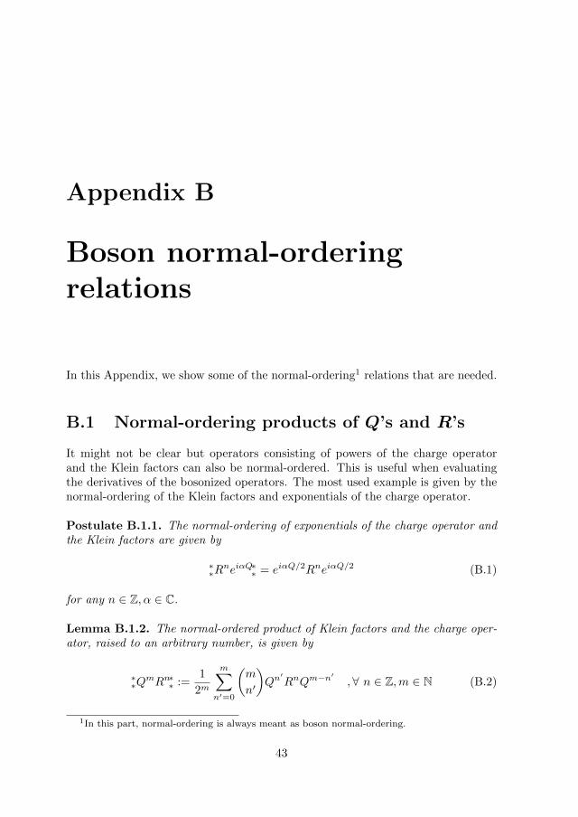
Appendix B
Boson normal-orderingrelations
In this Appendix, we show some of the normal-ordering1 relations that are needed.
B.1 Normal-ordering products of Q’s and R’s
It might not be clear but operators consisting of powers of the charge operatorand the Klein factors can also be normal-ordered. This is useful when evaluatingthe derivatives of the bosonized operators. The most used example is given by thenormal-ordering of the Klein factors and exponentials of the charge operator.
Postulate B.1.1. The normal-ordering of exponentials of the charge operator andthe Klein factors are given by
∗∗R
neiαQ∗∗ = eiαQ/2RneiαQ/2 (B.1)
for any n ∈ Z, α ∈ C.
Lemma B.1.2. The normal-ordered product of Klein factors and the charge oper-ator, raised to an arbitrary number, is given by
∗∗Q
mRn∗∗ :=1
2m
m∑n′=0
(m
n′
)Qn′RnQm−n
′,∀ n ∈ Z,m ∈ N (B.2)
1In this part, normal-ordering is always meant as boson normal-ordering.
43

44 Appendix B. Boson normal-ordering relations
Proof. Taking equation (B.1) and Taylor expanding with regard to α around 0 givesthat
∗∗R
n + iαQRn − α2
2Q2Rn − iα3
6Q3Rn +O(α4)∗∗ =(
1 + iα
2Q− α2
8Q2 − iα3
48Q3
)Rn(
1 + iα
2Q− α2
8Q2 − iα3
48Q3
)+O(α4)
(B.3)
which yields
∗∗QR
n∗∗ =
1
2(QRn +RnQ)
∗∗Q
2Rn∗∗ =1
4
(RnQ2 + 2QRnQ+Q2Rn
)∗∗Q
3Rn∗∗ =1
8
(RnQ3 + 3QRnQ2 + 3Q2RnQ+Q3Rn
)Generalizing the results for Q to the power of an arbitrary number gives equation(B.2).
B.2 Normal-ordering products of anyonoperators of arbitrary number
The products of N anyon operators has a very interesting correlation functionwhich corresponds to the ground-state of the Calogero-Sutherland (CS) model (c.f.Section 3.1.1). This is most easily seen if the product is normal-ordered. There arealso similar result for a multi-species product of anyon field operators.
We define w = (w1, w2, . . . , wN ) such that wk 6= wk′ ∀k 6= k′ and wk is givenby Eq. (2.25).
B.2.1 Product with the same species. Proof of Lemma 2.3.4
The proof is given by first normal-ordering the products of 2 and 3 anyon operatorsand then generalizing to a product of N operators.
2 anyon operators
The product of two anyon field operators can be written as
φν(w1)φν(w2) =(e−i
πLνν0x1QR
νν0 e−i
πLνν0x1Qe−i
πLνν0x2QR
νν0 e−i
πLνν0x2Q
)(1)×(
e−ν
∑n<0
1nρnw
n1
e−ν
∑n>0
1nρnw
n1
e−ν
∑m<0
1mρmw
m2
e−ν
∑m>0
1mρmw
m2
)(2)
(B.4)

B.2. Normal-ordering products of anyon operators of arbitrary number 45
Since the two parts of Eq. (B.4)((. . .)(1) and (. . .)(2)
)commute, they can be
normal-ordered separately. Normal-ordering the first part by using Eq. (1.34)gives
(. . .)(1) = e−iπLν
2(x1−x2)∗∗ (. . .)(1)
∗∗
where∗∗ (. . .)(1)
∗∗ = e−i
πLνν0(x1+x2)QR 2 νν0 e−i
πLνν0(x1+x2)Q
The second part can be normal-ordered by using equations (1.14) and (1.32), whichgives that
(. . .)(2) = e
[−ν
∑n>0
1nρnw
n1 ,−ν
∑m<0
1mρmw
m2
]∗∗ (. . .)(2)
∗∗
where
∗∗ (. . .)(2)
∗∗ = e
−ν∑n<0
1nρnw
n1
e−ν
∑m<0
1mρmw
m2
e−ν
∑n>0
1nρnw
n1
e−ν
∑m>0
1mρmw
m2
Summarizing the results gives that
φν(w1)φν(w2) = ∗∗φν(w1)φν(w2)∗∗ e
i πLν2(x2−x1)e
−ν2 ∑n>0
1nw
n1w−n2
= ∗∗φν(w1)φν(w2)∗∗ iw2,w1
∣∣∣∣w1
w2
∣∣∣∣ ν2
2(w1 − w2√w1w2
)ν2
So the final result becomes
φν(w1)φν(w2) = J ν(w1, w2)∗∗φν(w1)φν(w2)∗∗ (B.5)
where J ν is defined in Lemma 2.3.4.
Product of 3 anyon operators
Using equation (B.5) the product 3 anyon field operators can be written as
φν(w1)φν(w2)φν(w3) = J ν(w1, w2)∗∗φν(w1)φν(w2)∗∗φ
ν(w3) (B.6)
where
∗∗φν(w1)φν(w2)∗∗φ
ν(w3) =(e−i
πLνν0(x1+x2)QR 2 νν0 e−i
πLνν0(x1+x2)Q
×e−i πLνν0x3QRνν0 e−i
πLνν0x3Q
)(1)×(
e−ν
∑n<0
1nρn(wn1 +wn2 )
e−ν
∑n>0
1nρn(wn1 +wn2 )
e−ν
∑m<0
1mρmw
m3
e−ν
∑m>0
1mρmw
m3
)(2)
The two parts are again treated separately giving
(. . .)(1) = e−iπLν
2(x1+x2)eiπL 2ν2x3∗
∗ (. . .)(1)∗∗

46 Appendix B. Boson normal-ordering relations
(. . .)(2) = e
[−ν
∑n>0
1nρn(wn1 +wn2 ),−ν
∑m<0
1mρmw
m3
]∗∗ (. . .)(2)
∗∗
where∗∗ (. . .)(1)
∗∗ = e−i
πLνν0(x1+x2+x3)QR 3 νν0 e−i
πLνν0(x1+x2+x3)Q
∗∗ (. . .)(2)
∗∗ = e
−ν∑n<0
1nρn(wn1 +wn2 +wn3 )
e−ν
∑n>0
1nρn(wn1 +wn2 +wn3 )
Inserting the equations into Eq. (B.6) gives
φν(w1)φν(w2)φν(w3) = ∗∗φν(w1)φν(w2)φν(w3)∗∗ ×
J ν(w1, w2)e−iπLν
2(x1+x2−2x3)e−ν2 ∑
n>0
1n (wn1w
−n3 +wn2w
−n3 )
where
e−iπLν
2(x1+x2−2x3)e−ν2 ∑
n>0
1n (wn1w
−n3 +wn2w
−n3 )
=
(e−i
πLν
2(x1−x3)e−ν2 ∑
n>0
1nw
n1w−n3
)(e−i
πLν
2(x2−x3)e−ν2 ∑
n>0
1nw
n2w−n3
)
=
iw3,w1
∣∣∣∣w1
w3
∣∣∣∣ ν2
2(w3 − w1√w3w1
)ν2iw3,w2
∣∣∣∣w2
w3
∣∣∣∣ ν2
2(w3 − w2√w3w2
)ν2
which gives that
J ν(w1, w2)e−iπLν
2(x1+x2−2x3)e−ν2 ∑
n>0
1n (wn1w
−n3 +wn2w
−n3 )
= J ν(w1, w2, w3)
Summarizing the result yields
φν(w1)φν(w2)φν(w3) = J ν(w1, w2, w3)∗∗φν(w1)φν(w2)φν(w3)∗∗ (B.7)
where
∗∗φν(w1)φν(w2)φν(w3)∗∗ = e−i
πLνν0(x1+x2+x3)QR 3 νν0 e−i
πLνν0(x1+x2+x3)Q×
e−ν
∑n<0
1nρn(wn1 +wn2 +wn3 )
e−ν
∑n>0
1nρn(wn1 +wn2 +wn3 )
Product of N anyon operators
Generalizing the result for any N(∈ N). Equation (2.26) can be re-written as
Φν(w) = J ν(wkN−1k=1 )∗∗Φ
ν(wkN−1k=1 )∗∗ φ
ν(wN ) (B.8)

B.2. Normal-ordering products of anyon operators of arbitrary number 47
where
∗∗Φ
ν(wkN−1k=1 )∗∗ φ
ν(wN ) =e−i πLνν0(N−1∑k=1
xk
)Q
R (N−1) νν0 e−i πLνν0
(N−1∑k=1
xk
)Q
e−iπLνν0xNQR
νν0 e−i
πLνν0xNQ
(1)
×
e−ν N−1∑k=1
∑n<0
1nρnw
nk
e−ν
N−1∑k=1
∑n>0
1nρnw
nk
e−ν
∑m<0
1mρmw
mN
e−ν
∑m>0
1mρmw
mN
(2)
(B.9)
Using
(. . .)(1) = e−i πLν
2
(N−1∑k=1
xk
)eiπLν
2(N−1)xN ∗∗ (. . .)(1)
∗∗
(. . .)(2) = e
[−ν
N−1∑k=1
∑n>0
1nρnw
nk ,−ν
∑m<0
1mρmw
mN
]∗∗ (. . .)(2)
∗∗
gives that
∗∗Φ
ν(wkN−1k=1 )∗∗ φ
ν(wN ) =
N−1∏k′=1
iwN ,wk′
(∣∣∣∣wk′wN
∣∣∣∣ 12 wN − wk′√wNwk′
)ν2 ∗∗Φν(w)∗∗
where ∗∗Φν(w)∗∗ is defined in Eq. (2.27). This proves Lemma 2.3.4 since
J ν(wkN−1k=1 )
N−1∏k′=1
iwN ,wk′
(∣∣∣∣wk′wN
∣∣∣∣ 12 wN − wk′√wNwk′
)ν2
= ∏1≤k′<k≤N−1
iwk,wk′
(∣∣∣∣wk′wk
∣∣∣∣ 12 wk − wk′√wk′wk
)ν2N−1∏k′=1
iwN ,wk′
(∣∣∣∣wk′wN
∣∣∣∣ 12 wN − wk′√wNwk′
)ν2
= J ν(w)
B.2.2 Products of different species. Proof of Lemma 2.3.5
The treatment in Section B.2.1 can also be used to normal-order products of anyonfield operators with individual statistical parameters νk, where νk/ν0 ∈ Z ∀k.
The proof for Lemma 2.3.5 is very similar to the proof for Lemma 2.3.4, exceptchanging the statistic parameter to individual ones. It should not be necessary toprove it entirely. The method for a product of two anyon field operator, with differ-ent statistical parameters, is useful for calculating other relations, e.g. calculating(anti-)commutation relations, so it will be shown explicitly.

48 Appendix B. Boson normal-ordering relations
Normal-ordering a product of two anyon operators with differentspecies
The product is given by
φν1(w1)φν2(w2) =(e−i
πLν0ν1x1QR
ν1ν0 e−i
πLν0ν1x1Qe−i
πLν0ν2x2QR
ν2ν0 e−i
πLν0ν2x2Q
)(1)
×(e−ν1
∑n<0
1nρnw
n1
e−ν1
∑n>0
1nρnw
n1
e−ν2
∑m<0
1mρmw
m2
e−ν2
∑m>0
1mρmw
m2
)(2)
(B.10)
Normal-ordering the parts separately by
(. . .)(1) = e−iπLν1ν2x1ei
πLν1ν2x2∗
∗ (. . .)(1)∗∗
(. . .)(2) = e
[−ν1
∑n>0
1nρnw
n1 ,−ν2
∑m<0
1mρmw
m2
]∗∗ (. . .)(2)
∗∗
which gives that
φν1(w1)φν2(w2) = ∗∗φν1(w1)φν2(w2)∗∗
(e−i
πL (x1−x2)e
−∑n>0
1nw
n1w−n2
)ν1ν2= ∗∗φ
ν1(w1)φν2(w2)∗∗ iw2,w1
(∣∣∣∣w1
w2
∣∣∣∣ 12 w1 − w2√w1w2
)ν1ν2where
∗∗φν1(w1)φν2(w2)∗∗ = e−i
πLν0(ν1x1+ν2x2)QR
ν1+ν2ν0 e−i
πLν0(ν1x1+ν2x2)Q×
e−∑n<0
1nρn(ν1w
n1 +ν2w
n2 )e−∑n>0
1nρn(ν1w
n1 +ν2w
n2 )
such that〈∗∗φν1(w1)φν2(w2)∗∗〉 = δ ν1+ν2
ν0,0

Appendix C
Fock space equality
C.1 Boson completeness
As stated in Lemma 2.1.1, the basis vectors of the fermion Fock space F can berepresented in terms of the boson operators and the Klein factors. The Fock spacesspanned by the basis vectors
B(mn∞n=1 , ω) =
∞∏n=1
(a†n)mn
√mn!
RωΩ
or (C.1)
F (mk, nk∞k=0) =
∞∏k=0
(ψ∗k)mk (ψ−k−1)
nkΩ
where
a†n :=ρ−n√n
(C.2)
mn ∈ N0, mk, nk ∈ 0, 1, under the requirement that∑nmn <∞,∑
k
mk + nk <∞, are equal.
Since the boson operators can be expressed in terms of the fermion operators(c.f. (1.12)), the Fock space spanned by the bosonic vectors B(mn∞n=n , ω) is atleast a subspace of the fermion Fock space spanned by the vectors in equation (2.3).In order to show that the two Fock spaces are isomorphic, one can calculate thepartition function Z. The partition function are equal if every state in the Fockspace spanned by the F (mk, nk∞k=0) also occurs in the Fock space spanned by thebasis B(mn∞n=1 , ω).
49
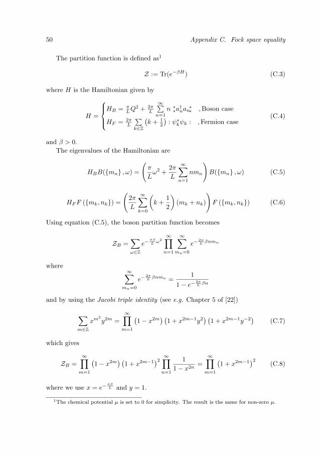
50 Appendix C. Fock space equality
The partition function is defined as1
Z := Tr(e−βH) (C.3)
where H is the Hamiltonian given by
H =
HB = π
LQ2 + 2π
L
∞∑n=1
n ∗∗a†nan∗∗ ,Boson case
HF = 2πL
∑k∈Z
(k + 1
2
): ψ∗kψk : ,Fermion case
(C.4)
and β > 0.
The eigenvalues of the Hamiltonian are
HBB(mn , ω) =
(π
Lω2 +
2π
L
∞∑n=1
nmn
)B(mn , ω) (C.5)
HFF (mk, nk) =
(2π
L
∞∑k=0
(k +
1
2
)(mk + nk)
)F (mk, nk) (C.6)
Using equation (C.5), the boson partition function becomes
ZB =∑ω∈Z
e−πβL ω2
∞∏n=1
∞∑mn=0
e−2πL βnmn
where∞∑
mn=0
e−2πL βnmn =
1
1− e− 2πL βn
and by using the Jacobi triple identity (see e.g. Chapter 5 of [22])
∑m∈Z
xm2
y2m =
∞∏m=1
(1− x2m
) (1 + x2m−1y2
) (1 + x2m−1y−2
)(C.7)
which gives
ZB =
∞∏m=1
(1− x2m
) (1 + x2m−1
)2 ∞∏n=1
1
1− x2n=
∞∏m=1
(1 + x2m−1
)2(C.8)
where we use x = e−πβL and y = 1.
1The chemical potential µ is set to 0 for simplicity. The result is the same for non-zero µ.

C.1. Boson completeness 51
Using Eq. (C.6), the fermion partition function becomes
ZF =
∞∏k=0
1∑mk,nk=0
e−2πβL (k+ 1
2 )(mk+nk) (C.9)
using
1∑mk,nk=0
e−2πβL (k+ 1
2 )(mk+nk) = 1 + 2e−2πβL (k+ 1
2 ) + e−2 2πβL (k+ 1
2 )
=(
1 + e−2πβL (k+1/2)
)2
=(1 + x2k+1
)2and
∞∏k=0
(1 + x2k+1
)2=
∞∏n′=1
(1 + x2(n′−1)+1
)2
=
∞∏n′=1
(1 + x2n′−1
)2
, n′ = k + 1
Inserting these relations into Eq. (C.9) and comparing to Eq. (C.8) shows that
ZF =
∞∏n′=1
(1 + x2n′−1
)2
= ZB

52

Appendix D
The W -current
D.1 The W1+∞ algebra
Definewsn := e−i
πLnxps−1e−i
πLnx , n ∈ Z , s ∈ N (D.1)
where x ∈ SL and p := −i ∂∂x . We can construct an operator valued generatingfunction (OVGF) by
wn(a) :=
∞∑s=1
(ia)s−1
(s− 1)!wsn = e−i
πLnxeiape−i
πLnx = e−i
πLnae−i
2πL nxeiap (D.2)
where a is a free parameter and equation (1.32) was used to obtain the final result.The W1+∞ algebra, which is the W∞ algebra with a central extension, is then
generated by the OVGFWn(a) := dΓ(wn(a)) (D.3)
satisfyingWn(a)Ω = 0 ∀n ≥ 0
The representation of the W1+∞ algebra is given by
[Wn(a),Wm(b)] = dΓ ([wn(a), wm(b)]) + c · iS(wn(a), wm(b)) (D.4)
where c is the central element satisfying
[Wn, c] = 0 c∗ = c
Using Eq. (1.5), the Schwinger term is given by
iS(wn(a), wm(b)) =∑k∈Z
((ek, P−wn(a)P+wm(b)P−ek)
− (ek, P−wm(b)P+wn(a)P−ek)) (D.5)
53

54 Appendix D. The W -current
where ek = ek(x) is the basis vector in L2(SL), defined as in Eq. (1.6), and obeythe following relations
P±ek = θ
(±(k +
1
2
))ek
e−i2πL nxek = ek−n
eiapek(x) = ek(x+ a) = e2πL i(k+ 1
2 )aek(x)
for all k ∈ Z and where θ(x) is the Heaviside step function (c.f. Appendix A).This gives that
P+wm(b)P−ek
=
θ(−k − 1
2 )θ(k −m+ 12 )ei
2πL (k−m2 + 1
2 )bek−m , if m < 0
0 , otherwise
Similarly P−wn(a)ek−m is only non-zero if n ≥ −m > 0. Using that the basisvectors are orthonormal, i.e. (ek, ek−n−m) = δn+m,0, yields∑
k∈Z(ek, P−wn(a)P+wm(b)P−ek)
=
−1∑
k=−nei
2πL (k+n
2 + 12 )·(a+b)δn,−m , if m < 0
0 , otherwise
=
δn,−m ·sin ( πLn(a+b))sin ( πL (a+b))
, if m < 0
0 otherwise
Similar treatment is done for the second part of Eq. (D.5) which yields∑k∈Z
(ek, P−wm(b)P+wn(a)P−ek)
=
−1∑
k=−mei
2πL (k+m
2 + 12 )·(a+b)δm,−n , if m > 0
0 , otherwise
=
−δm,−nsin( πLn(a+b))sin( πL (a+b))
, if m > 0
0 , otherwise
Combining these results gives
iS(wn(a), wm(b)) = δn,−msin(πLn(a+ b)
)sin(πL (a+ b)
) ,∀n,m ∈ Z (D.6)

D.1. The W1+∞ algebra 55
By using equation (1.32), it is fairly straightforward to compute the commuta-tion relation of the generating function
wn(a)wm(b) = e−iπLnae−i
2πL nxeiape−i
πLmbe−i
2πL mxeibp
= e−iπL (am−bn)wn+m(a+ b)
and
wm(b)wn(a) = e−iπLmbe−i
2πL mxeibpe−i
πLnae−i
2πL nxeiap
= eiπL (am−bn)wn+m(a+ b)
which yields
[wn(a), wm(b)] = 2i sin(πL
(bn− am))wn+m(a+ b)
Collecting the results yields that
[Wn(a),Wm(b)] = 2i sin(πL
(bn− am))Wn+m(a+ b) + c · δn,−m
sin(πLn(a+ b)
)sin(πL (a+ b)
)(D.7)
whereWn+m(a+ b) := dΓ (wn+m(a+ b))
Of particular interest are the oscillation operators and the generators of theVirasoro algebra, which are contained in the OVGF for c = 1.
The oscillation operator can be written as
ρn := dΓ(w1n) = lim
a↓0Wn(a) (D.8)
which gives that
[ρn, ρm] = lima↓0
limb↓0
[Wn(a),Wm(b)] = nδn,−m (D.9)
DefineLn := dΓ(w2
n) = lima↓0
(−i∂aWn(a)) (D.10)
which satisfies
[Ln, Lm] = lima,b↓0−∂a∂b [Wn(a),Wm(b)] = (n−m)Ln+m + δn,−m
n3 − n12
(D.11)
Eq. (D.11) is known as the Virasoro algebra and the operator Ln are then thegenerators of the Virasoro algebra.
Note that the Hamiltonian in (1 + 1) dimensions is given by H = L0 and Eq.(D.7) can be used to calculate the several important commutation relations.

56 Appendix D. The W -current
D.2 The Sugawara construction
In this Section, the real space representation of the operators contained in Eq. (D.3)are constructed for s ≤ 3.
Consider the point-split product of regularized fermion field operators, expressedin terms of bosonic operators as
ψ∗ε (x)ψε(x− a) =1
Le−i
πLxQRe−i
πLxQei
πL (x−a)QR−1ei
πL (x−a)Q
e−∑n<0
1nρne
i 2πLnxe−
2πL|n|ε
e−∑n<0
1nρne
i 2πLnxe−
2πL|n|ε
×
× e∑m<0
1mρme
i 2πLm(x−a)e−
2πL|m|ε
e
∑m>0
1mρme
i 2πLm(x−a)e−
2πL|m|ε
(D.12)
Making the point-split product into a boson normal-ordered form, by using theBCH formulas (equations (1.33) and (1.34)), yields
ψ∗ε (x)ψε(x− a) = eiπLae
∑n>0
1n e
i 2πLnae−
4πL|n|ε∗∗ψ∗ε (x)ψε(x− a)∗∗
where
∗∗ψ∗ε (x)ψε(x− a)∗∗ =
1
Lei
2πL aQe
∑n<0
1nρne
i 2πLnxe−
2πL|n|ε
(e−i
2πLna−1
)e
∑n>0
1nρne
i 2πLnxe−
2πL|n|ε
(e−i
2πLna−1
)
It is now possible to fermion normal-ordered the point-split product. Using
〈∗∗ψ∗ε (x)ψε(x− a)∗∗〉 =1
L
gives
:ψ∗ε (x)ψε(x− a) : = eiπLae
∑n>0
1n e
i 2πLnae−
4πL|n|ε (
∗∗ψ∗ε (x)ψε(x− a)∗∗ −
I
L
)=
eiπLa
1− ei 2πL (a+2iε)
(∗∗ψ∗ε (x)ψε(x− a)∗∗ −
I
L
)(D.13)
Since a fermion normal-ordered product is a well defined operator product, it ispossible to remove the regularization parameter, i.e. taking ε ↓ 0
:ψ∗(x)ψ(x− a) : =eiπLa
1− ei 2πL a
(∗∗ψ∗(x)ψ(x− a)∗∗ −
I
L
)(D.14)

D.3. The anyon W -current 57
Taylor expanding the r.h.s. of Eq. (D.14) gives that1
:ψ∗(x)ψ(x− a) : = ρ(x)− ia(π∗∗ρ(x)2∗
∗ +1
2i∗∗∂xρ(x)∗∗
)− a2
2
(4π2
3∗∗ρ(x)3∗
∗ −1
3∗∗∂
2xρ(x)∗∗ − 2πi∗∗ρ(x)∂xρ(x)∗∗ −
π2
6L2ρ(x)
)+O(a3) (D.15)
higher order terms are neglected since they are of little interest for this thesis.The fermion normal-ordered point-split product can also be written as
:ψ∗(x)ψ(x− a) : = :ψ∗(x)e−iapψ(x) : = :ψ∗(x)
( ∞∑n=0
(−ia)n
n!pn
)ψ(x) : (D.16)
Equations (D.15) and (D.16) gives
:ψ∗(x)ψ(x) : = ρ(x) (D.17)
Equation (D.17) gives exactly the same relation as equation (1.21). This relationis commonly referred to as the Kronig identity in the literatures.
The relation of interest (c.f. Eq. (C.4)) is
:ψ∗(x) p ψ(x) : = π∗∗ρ(x)2∗∗ +
1
2∗∗p ρ(x)∗∗ (D.18)
The l.h.s. of Eq. (D.18) is the position space representation for the generators ofthe Virasoro algebra. And
:ψ∗(x) p2 ψ(x) : =4π2
3∗∗ρ(x)3∗
∗ +1
3∗∗p
2ρ(x)∗∗ + 2π∗∗ρ(x) p ρ(x)∗∗ −π2
6L2ρ(x)
D.3 The anyon W -current
We defineWν(z; a) := Cν(a) : φν(zei
2πL a)φ−ν(z) : (D.19)
where Cν(a) is a normalization constant which plays an important role for higherorder corrections, as will be seen. Rewriting Eq. (D.19) in the bosonized form gives
Wν(z; a) =
N ν(a)
(e−i
2πL νν0aQe
−ν∑n<0
1nρnz
n(ei
2πLna−1
)e−ν
∑n>0
1nρnz
n(ei
2πLna−1
)− I
)(D.20)
where
N ν(a) :=i
2Lν2 cosν2(πaL
)tan
(πaL
) (D.21)
1Differentiation is a linear operation and therefore preserves normal-ordering

58 Appendix D. The W -current
The operator valued generating function for the anyon currents can then bedefined as
Wν(a) :=
∞∑s=1
(−ia)s−1
νs−2
(s− 1)!W ν,s = LResz
1
zWν(z; a) (D.22)
Lemma D.3.1. The operator Wν(a) is well defined on a dense subspace of F andleaves it invariant. The highest weight condition
Wν(a)Ω = 0 ∀ν ∈ R \ 0 ,∀a ∈ R
applies to the W ν,s operators as well by extension of Eq. (D.22).
Proof. See Ref. [19]
Using these generating functions, it is possible to calculate the analog of thefermion W -algebra for the anyons by calculating the commutation relation betweenthe generating function and an anyon operator (see Section D.3.2).
D.3.1 Construction of the W ν,s operator
Define
ρ(z) := ρ(z)− 1− ν0
LQ
with which we obtain (c.f. Eqs. (D.19) and (2.14))(e−i
2πL νν0aQe
−ν∑n<0
1nρnz
n(ei
2πLna−1
)e−ν
∑n>0
1nρnz
n(ei
2πLna−1
)− I
)
= exp
(−2πiν
∞∑k=1
ak
k!
(2πi
Lz∂z
)k−1
ρ(z)
)Introducing the operator ρ(z) defined as
ρ(z) :=1
L
∑n 6=0
ρnzn (D.23)
which is constructed such that it commutes with the Klein factors. We also definethe self-adjoint W s, s ∈ N, operators as
W s :=Ls−1
sResz
1
z∗∗ (ρ(z))
s ∗∗ (D.24)
which also commute with the Klein factors. The W s operators obey
W sRωΩ = 0 , ∀s ∈ N, ∀ω ∈ Z
These operators will serve as a more convenient way of expressing the otheroperators.

D.3. The anyon W -current 59
The fermion density operator can be written as
ρ(z) = ρ(z) +1
LQ
which gives that
ρ(z) = ρ(z) +ν0
LQ
The W ν,s operators, which are a formal power series of Wν(y; a), can then beexpressed as
W ν,1 = ν0Q (D.25)
W ν,2 =π
L
(2W 2 + ν2
0Q2)
(D.26)
W ν,3 =4π2
L2W 3 +
8π2ν0
L2QW 2 +
4π2ν30
3L2Q3 +
π2ν0
(2− 3ν2
)3ν2L2
Q (D.27)
Remark D.3.2. In the W ν,3 power series, there is a term − 4π2
νL∗∗ρ(z) z∂z ρ(z)∗∗ and it
is not obvious right away that this term vanishes. Upon integration and taking thelimit, that particular term becomes
∑n 6=0
n ∗∗ρ−nρn∗∗ =
∑n<0
nρnρ−n +∑n>0
nρ−nρn =∑n>0
nρ−nρn − nρ−nρn = 0 regardless of the vector it is applied to.
D.3.2 The W ν,s relations
The commutation relation between the generating function (Eq. (D.22)) and ananyon operator of the same species is given by taking equations (D.20) and (2.16)
[Wν(a), φν(w)] = L Resz [Wν(z; a), φν(w)] (D.28)
Boson normal-ordering each term of the commutation separately, using the tech-niques in Appendix B, gives that
Wν(z; a)φν(w) = ∗∗Wν(z; a)φν(w)∗∗e−i πLν
2ae−ν2
∞∑n=1
1n z
nw−n(ei
2πLna−1
)
and
φν(w)Wν(z; a) = ∗∗Wν(z; a)φν(w)∗∗ei πLν
2aeν2−∞∑n=−1
1n z
nw−n(ei
2πLna−1
)
The normalization constant of ∗∗W(z; a)φν(a)∗∗ expanded as a formal power seriesin terms of a would give N ν(a) ∝ 1
a + O(a). Since the relation of interest are up

60 Appendix D. The W -current
to the second power of a, it is only necessary to expand the exponent to the thirdpower. This gives that∑
n
1
n
( zw
)n (ei
2πL na − 1
)≈ 2πia
L
∑n
( zw
)n+
1
2
(2πia
L
)2∑n
n( zw
)n+
1
6
(2πia
L
)3∑n
n2( zw
)n+O(a4)
Using ∑n
n( zw
)n= z∂z
∑n
( zw
)n∑n
n2( zw
)n=(z∂z + z2∂2
z
)∑n
( zw
)nand Eqs. (1.24), (1.25) gives
[Wν(z; a), φν(w)] = ∗∗Γ(eiνF )∗∗(c0 + a · c1 + a2 · c2 +O(a3)
)(D.29)
where
Γ(eiνF ) := ∗∗Wν(z; a)φν(w)∗∗/N ν(a)
= e−iπLνν0(x+a)QR
νν0 e−i
πLνν0(x+a)Q×
e−ν
∑n<0
1nρn
(zn(e2πLina−1
)+wn
)e−ν
∑n>0
1nρn
(zn(e2πLina−1
)+wn
)(D.30)
andc0 :=
z
Lδ(z − w) (D.31)
c1 := − iπzL2
(ν2 − 1
)∂z (zδ(z − w)) (D.32)
c2 := −π2(ν2 − 1
) (ν2 − 2
)6L3
z(2∂2zz
2δ(z − w)− 2∂zzδ(z − w) + δ(z − w))
(D.33)Expanding the operator part of Eq. (D.28) gives that
1
ν
[W ν,1, φν(w)
]= LResz
1
zc0∗∗Γ(eiνF )∗∗
∣∣∣a=0
(D.34)
i[W ν,2, φν(w)
]= LResz
1
z
(c0(∂a∗∗Γ(eiνF )∗∗
) ∣∣∣a=0
+ c1∗∗Γ(eiνF )∗∗
∣∣∣a=0
)(D.35)
−[νW ν,3, φν(w)
]= LResz
1
z
(c0(∂2a∗∗Γ(eiνF )∗∗
) ∣∣∣a=0
+2c1(∂a∗∗Γ(eiνF )∗∗
) ∣∣∣a=0
+ 2c2∗∗Γ(eiνF )∗∗
∣∣∣a=0
)(D.36)

D.3. The anyon W -current 61
The short distance limit and derivatives of the operator part of Eq. (D.30) isgiven by
∗∗Γ(eiνF )∗∗
∣∣∣a=0
= φν(w)
∂a∗∗Γ(eiνF )∗∗ = −iν2π∗∗
(ρ(ze
2πL ia) +
ν0 − 1
LQ
)Γ(eiνF )∗∗
which gives that
(∂a∗∗Γ(eiνF )∗∗
) ∣∣∣a=0
= −2πiν∗∗
(ρ(z) +
ν0 − 1
LQ
)φν(w)∗∗
and
∂2a∗∗Γ(eiνF )∗∗ = −4π2ν2∗
∗
(ρ(ze
2πL ia) +
ν0 − 1
LQ
)2
Γ(eiνF )∗∗
− 2πiν∗∗ρ′(ze
2πL ia)Γ(eiνF )∗∗
where ρ′(ze2πL ia) = ∂aρ(ze
2πL ia) = 2π
L iz∂zρ(ze2πL ia). Which gives
(∂2a∗∗Γ(eiνF )∗∗
) ∣∣∣a=0
= −4π2ν2∗∗
(ρ(z) +
ν0 − 1
LQ
)2
φν(w)∗∗
+4π2
Lν∗∗ (z∂zρ(z))φν(w)∗∗
Lemma B.1.2 is used in order to obtain the results.Using Proposition 1.4.4 and partial integration gives
1
ν
[W ν,1, φν(w)
]= φν(w) (D.37)
i[W ν,2, φν(w)
]= −2πiν∗∗
(ρ(w) +
ν0 − 1
LQ
)φν(w)∗∗ =
2πi
Lw∂wφ
ν(w) (D.38)
where the second part of the integration, in Eq. (D.35), cancels out when doingpartial integration.
The sought after commutation relation is
−[νW ν,3, φν(w)
]=(
−4π2ν2∗∗
(ρ(w) +
ν0 − 1
LQ
)2
φν(w)∗∗ +4π2
Lν∗∗ (w∂wρ(w))φν(w)∗∗
)
+4π2
Lν(ν2 − 1
) ∗∗ (w∂wρ(w))φν(w)∗∗ −
π2(ν2 − 1
) (ν2 − 2
)3L2
φν(w)

62 Appendix D. The W -current
which can be re-written as
[νW ν,3, φν(w)
]=
4π2
L2(w∂w)
2φν(w)− 4π2
Lν(ν2 − 1
) ∗∗ (w∂wρ(w))φν(w)∗∗
+π2(ν2 − 1
) (ν2 − 2
)3L2
φν(w) (D.39)
Summarizing the results gives that
[W ν,s, φν ] = ν2−si1−s∂s−1
∂xs−1φν(w) , s = 1, 2
But for higher order terms there is a need for correction terms in order to obtain asimilar result.
Note that these relation hold as long as the operators and the anyon field oper-ator have the same statistical parameter ν.

Appendix E
Additional proofs
E.1 Proofs for Chapter 1
E.1.1 Proof of Proposition 1.4.4
Proof. 1. Let f(z) =∑n∈Z
fnzn±q, q ∈ Z be any formal distribution. Then
Reszf(z)δ(z − w) =∑n,m∈Z
fnwmReszz
n−m−1±q =∑n∈Z
fnwn±q = f(w)
2. 2 follows from 1.
3.
δ(z − w) =∑n∈Z
z−n−1wn =∑n∈Z
z−nwn−1 =∑n∈Z
znw−n−1 = δ(w − z)
4. Using
δ(z − w) =∑n∈Z
z−n−1wn =∑n∈Z
z−nwn+1
it is clear that Proposition 1.4.4 4 holds.
63

64 Appendix E. Additional proofs
E.1.2 Proof of Lemma 1.5.1
Proof. 1. Create an operator-valued function T (s) = e−sBAesB . Then
dTds
= e−sB (−B) ·AesB + e−sBAesBB = e−sB [A,B] esB = C
and all higher order derivatives vanish since [B,C] = 0. Taylor expandingT (s) gives
T (s) =
∞∑n=0
sn
n!
(dnTdsn
∣∣∣s=0
)= T (0) + s [A,B]
Taking the limits s = 1 yields Eq. (1.31). This relation implies[A, eB
]= AeB − eBA = eB
(e−BAeB −A
)= eBC
2. The relation is given by the Taylor expansion of f(A) and using (1.31)
3. Create a new operator-valued function Y(s) := esAesB , where
dYds
= esAAesB + esAesBB = Y(s) (A+B + sC)
which gives that
Y(s) = es(A+B)es2C/2
and taking the limit s = 1 yields Eq. (1.33). The final part is obtained byusing Eq. (1.32) in the special case of f(A) = eA.
E.2 Proofs for Chapter 2
E.2.1 Proof of Proposition 2.1.2
Proof. The density operator was the following commutation relation with thefermion field operators, which can be checked by using Eq. (1.21) and the CAR,[
ρ(w), ψ(∗)(z)]
= −(+)
z
Lδ(z − w)ψ(∗)(z)
where ρ(w) := 1L
∑n∈Z
ρnwn ∈ V
[[w,w−1
]]. A comparison of the commutation
relation to equations (1.20) and (1.31), would suggest that
ψ(∗)(z) ∝ exp
+(−)L
z∫dz′
1
z′ρ(z′)

E.2. Proofs for Chapter 2 65
The commutation relation between the charge operator and the fermion fieldoperators is given by [
Q,ψ(∗)(x)]
= −(+)ψ
(∗)(x)
Since it is known that the charge operator does not commute with the Klein factors,the commutation relation would suggest that ψ ∝ R−1, ψ∗ ∝ R.
The fermion operators could then be written as
ψ(z) ∝ R−1 exp
L z∫dz′
1
z′ρ(z′)
ψ∗(z) ∝ R exp
−L z∫dz′
1
z′ρ(z′)
E.2.2 Proof of Lemma 2.2.4
Proof. 1. Equation (2.17) is seen by comparing equations (1.18) and (2.16) withLemma 1.5.2.
2. The fermion density operator can be split into two parts such as ρ(w) =ρ(w) + Q
L where ρ, given by equation (D.23), is such that it commutes withthe Klein factors. Using Eq. (1.31) gives that
[ρ(w), φν(z)] =
([P−ρ(w),−ν
∑m>0
ρmmzm
]
+
[P+ρ(w),−ν
∑m<0
ρmmzm
])φν(z)
which gives
[ρ(w), φν(z)] =ν
L(zδ(z − w)− 1)φν(z)
E.2.3 Proof of Proposition 2.3.2
Proof. Boson normal-ordering the products yields1
φν(w)φ−1ν (z) = e−
12 ln|wz |
√w
ze
∑n>0
1nw
nz−n∗∗φν(w)φ−
1ν (z)∗∗
= iz,w e−12 ln|wz |√zw 1
z − w∗∗φν(w)φ−
1ν (z)∗∗
1For more details see Appendix B

66 Appendix E. Additional proofs
and
φ−1ν (z)φν(w) = e
12 ln|wz |
√z
we
∑n>0
1nw−nzn ∗
∗φ− 1ν (z)φν(w)∗∗
= −iw,ze12 ln|wz |√zw 1
z − w∗∗φ− 1ν (z)φν(w)∗∗
where
iz,w ln∣∣∣wz
∣∣∣ < 0
iw,z ln∣∣∣wz
∣∣∣ > 0
and∗∗φν(w)φ−
1ν (z)∗∗ = ∗∗φ
− 1ν (z)φν(w)∗∗
So the anti-commutation relation becomesφν(w), φ−
1ν (z)
= e
12 |ln|wz ||√zw
(iz,w
1
z − w− iw,z
1
z − w
)∗∗φν(w)φ−
1ν (z)∗∗
= e12 |ln|wz ||√zw δ(z − w) ∗∗φ
ν(w)φ−1ν (z)∗∗ = zδ(z − w) ∗∗φ
ν(w)φ−1ν (z)∗∗ (E.1)
where Proposition 1.4.4 2 is used in order to obtain the final result.
E.3 Proofs for Chapter 3
E.3.1 Proof of Lemma 3.2.4
Proof. Using Eqs. (2.16), (1.31) and that the C operator commutes with the chargeoperators and the Klein factors yields that
Cφν(w) =4π2
L2
∑n>0
nρ−nφν(w)ρn +
4π2
L2
∑n>0
nρ−n
[ρn,−ν
∑m<0
1
mρmw
m
]φν(w)
= ∗∗Cφν(w)∗∗ +
4π2
L2ν∑n>0
nρ−nw−nφν(w)
and
φν(w)C =4π2
L2
∑n>0
nρ−nφν(w)ρn +
4π2
L2
∑n>0
nφν(w)
[−ν
∑m>0
1
mρmw
m, ρ−n
]ρn
= ∗∗φν(w)C∗∗ −
4π2
L2νφν(w)
∑n>0
nρnwn
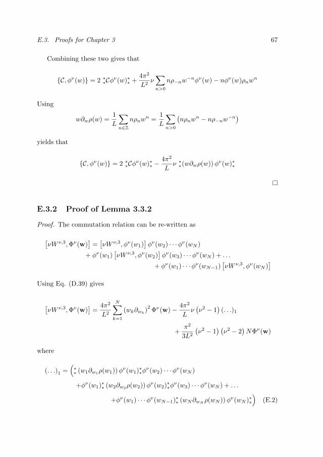
E.3. Proofs for Chapter 3 67
Combining these two gives that
C, φν(w) = 2 ∗∗Cφν(w)∗∗ +4π2
L2ν∑n>0
nρ−nw−nφν(w)− nφν(w)ρnw
n
Using
w∂wρ(w) =1
L
∑n∈Z
nρnwn =
1
L
∑n>0
(nρnw
n − nρ−nw−n)
yields that
C, φν(w) = 2 ∗∗Cφν(w)∗∗ −4π2
Lν ∗∗(w∂wρ(w))φν(w)∗∗
E.3.2 Proof of Lemma 3.3.2
Proof. The commutation relation can be re-written as
[νW ν,3,Φν(w)
]=[νW ν,3, φν(w1)
]φν(w2) · · ·φν(wN )
+ φν(w1)[νW ν,3, φν(w2)
]φν(w3) · · ·φν(wN ) + . . .
+ φν(w1) · · ·φν(wN−1)[νW ν,3, φν(wN )
]Using Eq. (D.39) gives
[νW ν,3,Φν(w)
]=
4π2
L2
N∑k=1
(wk∂wk)2
Φν(w)− 4π2
Lν(ν2 − 1
)(. . .)1
+π2
3L2
(ν2 − 1
) (ν2 − 2
)NΦν(w)
where
(. . .)1 =(∗∗ (w1∂w1
ρ(w1))φν(w1)∗∗φν(w2) · · ·φν(wN )
+φν(w1)∗∗ (w2∂w2ρ(w2))φν(w2)∗∗φ
ν(w3) · · ·φν(wN ) + . . .
+φν(w1) · · ·φν(wN−1)∗∗ (wN∂wNρ(wN ))φν(wN )∗∗
)(E.2)

68 Appendix E. Additional proofs
Eq. (E.2) expressed in terms of the oscillation operators is
(. . .)1 =1
L
∑n<0
nρnwn1 Φν(w) +
1
Lφν(w1)
∑n>0
nwn1 ρnφν(w2) · · ·φν(wN )
+1
Lφν(w1)
∑n<0
nρnwn2φ
ν(w2)φν(w3) · · ·φν(wN )
+1
Lφν(w1)φν(w2)
∑n>0
nρnwn2φ
ν(w3) · · ·φν(wN ) + . . .
+ φν(w1) · · ·φν(wN−1)∑n<0
nρnwnNφ
ν(wN ) + Φν(w)∑n>0
nρnwnN
Using Eq. (1.31) gives
(. . .)1 =
N∑k=1
(wk∂wkρ(wk)) ∗ Φν(w)
+
(1
L
N−1∑k′=1
N∑k=k′+1
∑n>0
nwnk′
[ρn,−ν
∑m<0
1
mρmw
mk
])Φν(w)
+
1
L
N∑k′=2
k′−1∑k=1
∑n<0
nwnk′
[−ν
∑m>0
1
mρmw
mk , ρn
]Φν(w)
which becomes
(. . .)1 =N∑k=1
(wk∂wkρ(wk)) ∗ Φν(w) +2ν
L
∑k′<k
wkwk′
(wk − wk′)2 Φν(w)
Collecting the results yields Eq. (3.34).
E.3.3 Proof of Lemma 3.3.3
Proof.
Remark E.3.1. The definition of boson normal-ordering and the definition of theC operator, given in Eq. (3.16) implies that that the anti-commutation relation ofthe C operator and the many-body anyon field operator Φν(w) is equivalent to theanti-commutation relation of the C operator and the boson normal-ordered form ofthe many-body anyon field operator, given in Eq. (2.27), due to Lemma 2.3.4.

E.3. Proofs for Chapter 3 69
Using Eq. (1.31) gives that
C∗∗Φν(w)∗∗ = C ∗ ∗∗Φν(w)∗∗ +4π2
L2
∑n>0
nρ−n
[ρn,−ν
N∑k=1
∑m<0
1
mρmw
mk
]· ∗∗Φν(w)∗∗
= C ∗ ∗∗Φν(w)∗∗ −4π2
L2ν
N∑k=1
∑m<0
mρmwmk∗∗Φ
ν(w)∗∗ (E.3)
where C ∗ ∗∗Φν(w)∗∗ = ∗∗CΦν(w)∗∗ and
∗∗Φ
ν(w)∗∗C = C ∗ ∗∗Φν(w)∗∗ + ∗∗Φν(w)∗∗ ·
4π2
L2
∑n>0
n
[−ν
N∑k=1
∑m>0
1
mρmw
mk , ρ−n
]ρn
= C ∗ ∗∗Φν(w)∗∗ − ∗∗Φν(w)∗∗ ·4π2
L2ν
N∑k=1
∑m>0
mρmwmk (E.4)
Combining Eqs. (E.3) and (E.4) gives that
C, ∗∗Φν(w)∗∗ = 2C ∗ ∗∗Φν(w)∗∗
− 4π2
L2ν
N∑k=1
∑m<0
mρmwmk∗∗Φ
ν(w)∗∗ − ∗∗Φν(w)∗∗ ·4π2
L2ν
N∑k=1
∑m>0
mρmwmk
= 2C ∗ ∗∗Φν(w)∗∗ −4π2
L2ν
N∑k=1
(wk∂wkρ(wk)) ∗ ∗∗Φν(w)∗∗
E.3.4 Proof of Corollary 3.3.6
Proof. Using Lemma 2.3.4 the correlation function can be rewritten as
F0(w) := 〈ηCS,Φν(w)Ω〉 = J ν(w) 〈ηCS,
∗∗Φ
ν(w)∗∗Ω〉
where
〈ηCS,∗∗Φ
ν(w)∗∗Ω〉 =⟨R−N
νν0 e−i πLνν0
N∑k=1
xkQRN
νν0 e−i πLνν0
N∑k=1
xkQe−ν
N∑k=1
∑n<0
1nρnw
nk
e−ν
N∑k=1
∑n>0
1nρnw
nk
⟩
=
⟨R−N
νν0 e−i πLνν0
N∑k=1
xkQRN
νν0
⟩= e−i πLν
2NN∑k=1
xk
This result is obtained since the oscillation operator ρn commutes with the chargeoperator and the Klein factors for n 6= 0 and by using Eq. (1.13).

70 Appendix E. Additional proofs
Comparing F0(w) and the GS wavefunction of the CS model (Eq. (3.1)) showsthat the correlation function F0(w) can be written as
F0(w) = cψ0(w)g(w)
where c ∈ C is a constant and
g(w) = e−i πLν
2NN∑k=1
xk=
N∏k=1
(wk|wk|
)−Nν22
So the CS Hamiltonian (c.f. Eq. (3.2)) acting on the correlation function F0(w)gives
HNF0(w) = c (HNψ0(w)) g(w)
+8π2
L2c
N∑k′=1
(wk′∂wk′ψ0(w)
) (wk′∂wk′ g(w)
)+
4π2
L2cψ0(w)
N∑k′=1
(wk′∂wk′
)2g(w) (E.5)
whereHNψ0(w) = E0ψ0(w)
N∑k′=1
(wk′∂wk′ψ0(w)
)wk′∂wk′ N∏k=1
(wk|wk|
)−Nν22
= 0
andN∑k′=1
(wk′∂wk′
)2g(w) = g(w)
ν4N2
4
N∑k′=1
1 = g(w)N3ν4
4
which gives that
HNF0(w) = E0F0(w) +4π2
L2
N3ν4
4F0(w) = ECSF0(w)
E.4 Proofs for Chapter 4
E.4.1 Proof of Theorem 4.1.2
Proof. The commutation can be re-written as[Hν,3, ϕν(z,w)
]=[Hν,3,Φ− 1
ν (z)Φν(w)]
=[Hν,3,Φ− 1
ν (z)]
Φν(w) + Φ−1ν (z)
[Hν,3,Φν(w)
](E.6)

E.4. Proofs for Chapter 4 71
Proposition 3.3.4 gives that
Φ−1ν (z)
[Hν,3,Φν(w)
]= Φ−
1ν (z)
(4π2
L2
N∑k=1
(wk∂wk)2Φν(w)
−4π2
L22ν2
(ν2 − 1
) ∑k′<k
wkwk′
(wk − wk′)2 Φν(w)
−2(ν2 − 1
)(C ∗ Φν(w)− Φν(w)C)
)which yields
Φ−1ν (z)
[Hν,3,Φν(w)
]=
4π2
L2
N∑k=1
(wk∂wk)2ϕν(z,w)
− 4π2
L2
∑k′<k
wkwk′
(wk − wk′)2 ϕν(z,w)
− 2(ν2 − 1
) (Φ−
1ν (z) (C ∗ Φν(w))− ϕν(z,w)C
)By using Lemma 3.2.6, the first commutation in Eq. (E.6) becomes
[Hν,3,Φ− 1
ν (z)]
Φν(w) = −ν2[H− 1
ν ,3,Φ−1ν (z)
]Φν(w)
+4π2
L2
(ν4 − 1
)ν2
[H− 1
ν ,1,Φ−1ν (z)
]Φν(w)
where [H− 1
ν ,1,Φ−1ν (z)
]= MΦ−
1ν (z)
and
[H− 1
ν ,3,Φ−1ν (z)
]=
4π2
L2
M∑j=1
(zj∂zj
)2Φ−
1ν (z)
− 4π2
L2
2
ν2
(1
ν2− 1
)∑j′<j
zjzj′
(zj − zj′)2 Φ−1ν (z)
− 2
(1
ν2− 1
)(C ∗ Φ−
1ν (z)− Φ−
1ν (z)C
)

72 Appendix E. Additional proofs
by using Proposition 3.3.4. This gives that
− ν2[H− 1
ν ,3,Φ−1ν (z)
]Φν(w) = −4π2
L2ν2
M∑j=1
(zj∂zj
)2ϕν(z,w)
− 4π2
L2
2
ν2
(ν2 − 1
)∑j′<j
zjzj′
(zj − zj′)2 ϕν(z,w)
− 2(ν2 − 1
) ((C ∗ Φ−
1ν (z)
)Φν(w)− Φ−
1ν (z)CΦν(w)
)Combing the results, so far, yields
[Hν,3, ϕν(z,w)
]=
4π2
L2
N∑k=1
(wk∂wk)2ϕν(z,w)− 4π2
L2ν2
M∑j=1
(zj∂zj
)2ϕν(z,w)
− 4π2
L2
(ν2 − 1
)2ν2∑k′<k
wkwk′
(wk − wk′)2 +2
ν2
∑j′<j
zjzj′
(zj − zj′)2
ϕν(z,w)
+4π2
L2M
(ν4 − 1
)ν2
ϕν(z,w)
− 2(ν2 − 1
) ((C ∗ Φ−
1ν (z)
)Φν(w) + Φ−
1ν (z) (C ∗ Φν(w))
−Φ−1ν (z)CΦν(w)− ϕν(z,w)C
)(E.7)
We use Remark E.3.1 when evaluating the final part of Eq. (E.7).
(C ∗ ∗∗Φ−
1ν (z)∗∗
)∗∗Φ
ν(w)∗∗ =4π2
L2
∑n>0
nρ−n∗∗Φ− 1ν (z)∗∗ρn
∗∗Φ
ν(w)∗∗
=4π2
L2
∑n>0
nρ−n∗∗Φ− 1ν (z)∗∗
∗∗Φ
ν(w)∗∗ρn +4π2
L2
∑n>0
nρ−n∗∗Φ− 1ν (z)∗∗ [ρn,
∗∗Φ
ν(w)∗∗]
= C ∗(∗∗Φ− 1ν (z)∗∗
∗∗Φ
ν(w)∗∗
)+
4π2
L2
∑n>0
nρ−n∗∗Φ− 1ν (z)∗∗
[ρn,−ν
N∑k=1
∑m<0
1
mρmw
mk
]∗∗Φ
ν(w)∗∗
= C ∗(∗∗Φ− 1ν (z)∗∗
∗∗Φ
ν(w)∗∗
)+
4π2
L2ν
N∑k=1
nρ−nw−nk∗∗Φ− 1ν (z)∗∗
∗∗Φ
ν(w)∗∗
Un-normal-ordering the anyon many-body operators gives that(C ∗ Φ−
1ν (z)
)Φν(w) = C ∗ ϕν(z,w)− 4π2
L2ν
N∑k=1
∑n<0
nρnwnkϕ
ν(z,w) (E.8)

E.4. Proofs for Chapter 4 73
Using the exact same method gives that
Φ−1ν (z) (C ∗ Φν(w)) = C ∗ ϕν(z,w) + ϕν(z,w) · 4π2
L2
1
ν
M∑j=1
∑n>0
nρnznj (E.9)
and finally
∗∗Φ− 1ν (z)∗∗C∗∗Φν(w)∗∗ =
4π2
L2
∑n>0
n∗∗Φ− 1ν (z)∗∗ρ−nρn
∗∗Φ
ν(w)∗∗
=4π2
L2
∑n>0
n∗∗Φ− 1ν (z)∗∗ρ−n (∗∗Φ
ν(w)∗∗ρn + [ρn,∗∗Φ
ν(w)∗∗])
= ∗∗Φ− 1ν (z)∗∗ (C ∗ ∗∗Φν(w)∗∗) +
4π2
L2ν
N∑k=1
∑n>0
nw−nk∗∗Φ− 1ν (z)∗∗ρ−n
∗∗Φ
ν(w)∗∗
Using Eq. (E.9) gives that
∗∗Φ− 1ν (z)∗∗C∗∗Φν(w)∗∗ = C ∗
(∗∗Φ− 1ν (z)∗∗
∗∗Φ
ν(w)∗∗
)+ ∗∗Φ
− 1ν (z)∗∗
∗∗Φ
ν(w)∗∗ ·4π2
L2
1
ν
M∑j=1
∑n>0
nρnznj
+4π2
L2ν
N∑k=1
∑n>0
nρ−nw−nk∗∗Φ− 1ν (z)∗∗
∗∗Φ
ν(w)∗∗
+4π2
L2
N∑k=1
∑n>0
nw−nk
[∗∗Φ− 1ν (z)∗∗, ρ−n
]∗∗Φ
ν(w)∗∗
Which yields
Φ−1ν (z)CΦν(w) = C ∗ ϕν(z,w)
+ ϕν(z,w) · 4π2
L2
1
ν
M∑j=1
∑n>0
nρnznj −
4π2
L2
N∑k=1
∑n<0
nρnwnk ϕ
ν(z,w)
+4π2
L2
N∑k=1
M∑j=1
∑n>0
nznj w−nk ϕν(z,w)
Collecting the results yields(C ∗ Φ−
1ν (z)
)Φν(w) + Φ−
1ν (z) (C ∗ Φν(w))− Φ−
1ν (z)CΦν(w) =
C ∗ ϕν(z,w)− 4π2
L2
N∑k=1
M∑j=1
∑n>0
nznj w−nk ϕν(z,w)

74 Appendix E. Additional proofs
where ∑n>0
nznj w−nk =
wkzj
(wk − zj)2
E.4.2 Proof of Theorem 4.2.1
Consider the Fock space inner product⟨η,Hν,3ϕν(z,w)Ω
⟩=⟨Hν,3η, ϕν(z,w)Ω
⟩(E.10)
Using Eq. (3.21) gives that the l.h.s. of Eq. (E.10) can be written as⟨η,Hν,3ϕν(z,w)Ω
⟩=⟨η,[Hν,3, ϕν(z,w)
]Ω⟩
Theorem 4.1.2 gives that the l.h.s. of Eq. (E.10) equals the dCS differential operatoraction on the correlation function Fη(z,w) with an additional term (c.f. Eq. (4.3)),i.e. ⟨
η,Hν,3ϕν(z,w)Ω⟩
=
(HN,M +
π2
3L2
ν4 − 1
ν2M
)〈η, ϕν(z,w)Ω〉
The r.h.s. of Eq. (E.10) equals EFη(z,w) since η is an eigenvector of the Hν,3operator with eigenvalue E .
E.4.3 Proof of Corollary 4.2.2
Proof. Lemma 2.3.6 and Eq. (3.33) gives that the inner product can be written as
〈ηdCS, ϕν(z,w)Ω〉 =
⟨R−(N νν0−M 1
νν0
)ϕν(z,w)
⟩=
J− 1ν (z)J ν(w)
N∏k=1
M∏j=1
∣∣∣∣wkzj∣∣∣∣ 12 √wkzjwk − zj
⟨R−(N νν0−M 1
νν0
)∗∗ϕ
ν(z,w)∗∗
⟩where⟨
R−(N νν0−M 1
νν0
)∗∗ϕ
ν(z,w)∗∗
⟩=⟨
R−(N νν0−M 1
νν0
)e−i πLν0
(νN∑k=1
xk− 1ν
M∑j=1
yj
)Q
RNνν0−M 1
νν0
⟩=
e−i πLν0
(N νν0−M 1
νν0
)(νN∑k=1
xk− 1ν
M∑j=1
yj
)
= e−i πLν
−2(Nν2−M)
(ν2
N∑k=1
xk−M∑j=1
yj
)

E.4. Proofs for Chapter 4 75
The correlation function F0(z,w) can be rewritten as
F0(z,w) = cψ0(z,w)g(z,w)
where c is a constant, ψ0(z,w) is the dGS eigenfunction, and
g(z,w) = e−i πL
(Nν2−Mν2
)(ν2
N∑k=1
xk−M∑j=1
yj
)
=
N∏k=1
M∏j=1
(wk|wk|
)−Nν2−M2(zj|zj |
)Nν2−M2ν2
The dCS differential operator acting on the correlation function is
HN,M F0(z,w) = c(HN,M ψ0(z,w)
)g(z,w)
+8π2
L2c
N∑k=1
(wk∂wk ψ0(z,w)
)(wk∂wkg(z,w))
+ cψ0(z,w)4π2
L2
N∑k=1
(wk∂wk)2g(z,w)− 8π2
L2ν2
M∑j=1
(zj∂zj ψ0(z,w)
) (zj∂zjg(z,w)
)− cψ0(z,w)
4π2
L2ν2
M∑j=1
(zj∂zj
)2g(z,w)
where
HN,M ψ0(z,w) = E0ψ0(z,w)
N∑k=1
(wk∂wk ψ0(z,w)
)(wk∂wkg(z,w))
− ν2M∑j=1
(zj∂zj ψ0(z,w)
) (zj∂zjg(z,w)
)= 0
and
N∑k=1
(wk∂wk)2g(z,w) = g(z,w)
N∑k=1
(Nν2 −M
)24
= g(z,w) =N(Nν2 −M
)24
M∑j=1
(zj∂zj
)2g(z,w) = g(z,w)
M∑j=1
(Nν2 −M
2ν2
)2
= g(z,w)M(Nν2 −M
)24ν4

76 Appendix E. Additional proofs
which gives
N∑k=1
(wk∂wk)2g(z,w)− ν2
M∑j=1
(zj∂zj
)2g(z,w) =
(Nν2 −M
)34ν2

Bibliography
[1] F. Calogero, Solution of the one-dimensional N-body problems with quadraticand/or inversely quadratic pair potentials, J. Math. Phys 12, 419 (1971).
[2] F. Calogero, Ground state of a one-dimensional N-body system, J. Math. Phys10, 2197 (1969).
[3] B. Sutherland, Exact results for a quantum many-body problem in one dimen-sion, Phys. Rev. A 4 (1971).
[4] O. Chalykh, M. Feigin and A. Veselov, New integrable generalizations of theCalogero-Moser quantum problems, J. Math. Phys 39, 695 (1998).
[5] A. Sergeev and A. Veselov, Deformed quantum Calogero-Moser problems andLie superalgebras, Commun. Math. Phys 245, 249 (2004).
[6] E. Langmann and M. Hallnas, A unified construction of generalized classi-cal polynomials associated with operators of Calogero-Sutherland type, Constr.Approx. 31, 309 (2010).
[7] D. C. Tsui, H. L. Stormer and A. C. Gossard, Two-Dimensional Magneto-transport in the Extreme Quantum Limit, Phys. Rev. Lett. 48, 1559 (1982).
[8] K. von Klitzing, The Quantum Hall effect, edited by B. Doucot et al., PoincareSeminar 2004, BirkHauser.
[9] R. Laughlin, Anomalous Quantum Hall Effect: An incompressible QuantumFluid with Fractionally Charged Excitations, Phys. Rev. Lett. 50, 1395 (1983).
[10] F. D. M. Haldane, Fractional Quantization of the Hall Effect: A Hierarchy ofIncompressible Quantum Fluid States, Phys. Rev. Lett. 51, 605 (1983).
[11] B. Halperin, Theory of the quantized Hall conductance, Helv. Phys. Acta 56,75 (1983).
[12] J. K. Jain, Composite-fermion approach for the fractional quantum Hall effect,Phys. Rev. Lett. 63, 199 (1989).
77

78 Bibliography
[13] E. Witten, Quantum field theory and the Jones polynomials, Commun. Math.Phys 121, 351 (1989).
[14] X. G. Wen, Chiral Luttinger liquid and the edge excitations in the fractionalquantum Hall states, Phys. Rev. B 41, 12838 (1990).
[15] X. G. Wen, Gapless boundary excitations in the quantum Hall states and inthe chiral spin states, Phys. Rev. B 43, 11025 (1991).
[16] J. Leinaas and J. Myrheim, On the theory of identical particles, Nuovo Com.B 37, 1 (1977).
[17] F. Wilczek, Quantum Mechanics of Fractional-Spin Particles, Phys. Rev. Lett.49, 957 (1982).
[18] S. Iso, Anyon basis of c=1 conformal field theory, Nucl. Phys. B 443, 581(1995).
[19] E. Langmann and A. Carey, Loop Groups, Anyons and the Calogero-Sutherlandmodel, Commun. Math. Phys 201, 1 (1999).
[20] S. Iso and S. J. Rey, Collective field theory of the fractional quantum Hall edgestate and the Calogero-Sutherland model, Phys. Lett. B 352, 111 (1995).
[21] C. Nayak et al., Non-Abelian anyons and topological quantum computation,Rev. Mod. Phys. 80, 1083 (2008).
[22] V. Kac, Vertex algebras for beginners, 2nd ed. (American Mathematical Soci-ety, 1997).
[23] A. Carey and S. Ruijsenaars, On fermion gauge groups, current algebra andthe Kac-Moody algebras, Acta Appl. Math 10 (1987).
[24] E. Langmann and H. Grosse, A super-version of quasi-free second quantization.I. Charged particles, J. Math. Phys 33 (1992).
[25] S. Ruijsenaars, On Bogoliubov transformation for systems of relativisticcharged particles, J. Math. Phys 18, 851 (1994).
[26] E. Langmann, Topics in quantum field theory, Lecture notes for a course givenat KTH 2003 (unpublished).
[27] J. von Delft and H. Schoeller, Bosonization for beginners – refermionizationfor experts, Annalen Phys. 7, 1998, arXiv:cond-mat/9805275v3.
[28] F. Calogero, Solution of a three-body problem in one dimension, J. Math. Phys10, 2191 (1969).
[29] B. Sutherland, Exact results for a quantum many-body problem in ine dimen-sion. II, Phys. Rev. A 5 (1972).