Symplectic geometry and Calogero-Mosersystems

Lukas RødlandSupervisor: Luigi Tizzano

Subject reader: Maxime ZabzineBachelor of Science Degree in Physics

Uppsala University

June 25, 2015

Abstract

We introduce some basic concepts from symplectic geometry, clas-sical mechanics and integrable systems. We use this theory to showthat the rational and the trigonometric Calogero-Moser systems, thatis the Hamiltonian systems with Hamiltonian H =

∑ni=1 p

2i−∑

j 6=i1

(xi−xj)2

and H =∑

i pi +∑

i 6=j1

4 sin2((xi−xj)/2)respectively are integrable sys-

tems. We do this using symplectic reduction on T ∗Matn(C).

Sammanfattning

Vi presenterar nagra grundlaggande ideer fran symplektisk ge-ometri, klassisk mekanik och integrabla system. Vi anvander dennateori for att visa att rationella och trigonometriska Calogero-Mosersystem, det vill saga hamiltonska system med hamiltonoperator H =∑n

i=1 p2i −

∑j 6=i

1(xi−xj)2 respektive H =

∑i pi +

∑i 6=j

14 sin2((xi−xj)/2)

respektive ar integrerbara system. Vi gor detta genom att anvandasymplektisk reduktion pa T ∗Matn(C).

1

Contents

1 Introduction 3

2 Symplectic geometry 42.1 Symplectic manifolds . . . . . . . . . . . . . . . . . . . . . . . 42.2 Isotopies and vector fields . . . . . . . . . . . . . . . . . . . . 7

3 Hamiltonian mechanics 83.1 Hamiltonian and symplectic vector fields . . . . . . . . . . . . 83.2 Brackets . . . . . . . . . . . . . . . . . . . . . . . . . . . . . . 93.3 Classical mechanics . . . . . . . . . . . . . . . . . . . . . . . . 103.4 Integrable systems . . . . . . . . . . . . . . . . . . . . . . . . 12

4 Moment maps 134.1 Lie groups . . . . . . . . . . . . . . . . . . . . . . . . . . . . . 134.2 Smooth actions . . . . . . . . . . . . . . . . . . . . . . . . . . 134.3 Orbit spaces . . . . . . . . . . . . . . . . . . . . . . . . . . . . 144.4 Adjoint and coadjoint representation . . . . . . . . . . . . . . 154.5 Moment and comoment maps . . . . . . . . . . . . . . . . . . 16

5 Symplectic reduction 185.1 Marsden-Weinstein-Meyer theorem . . . . . . . . . . . . . . . 185.2 Noether principle . . . . . . . . . . . . . . . . . . . . . . . . . 185.3 Elementary theory of reduction . . . . . . . . . . . . . . . . . 195.4 Reduction at other levels . . . . . . . . . . . . . . . . . . . . . 20

6 Calogero-Moser systems 206.1 Calogero-Moser space . . . . . . . . . . . . . . . . . . . . . . . 216.2 Rational Calogero-Moser system . . . . . . . . . . . . . . . . . 246.3 Trigonometric Calogero-Moser system . . . . . . . . . . . . . . 26

7 Conclusions 28

References 28

2

1 Introduction

One of the big turning points in the history of classical mechanics came whenPoincare showed that most systems cannot be solved exactly. Even simplesystems, as the three-body problem in three dimensions does not have anexact solution. Those systems that have a exact solution is called Liouvilleintegrable systems, or just integrable systems. Even if most realistic systemsare not integrable, there is still interesting to study them.

One group of these systems is the Calogero-Moser systems. They are one-dimensional N-body problems with a pairwise potential. Francesco Calogeroshowed in 1971 that the quantum mechanical system with Hamiltonian func-tion

H =N∑i=1

p2i −∑j 6=i

1

(xi − xj)2.

is integrable in the quantum mechanical sense. This is the system with Nparticles on a line with a pairwise potential which depends of the distancesquared between each pair of particles and is known as the rational Calogero-Moser system. In 1971 Sutherland showed that the system with potentialproportional to sin−2(xi − xj) also is integrable as a quantum mechanicalsystem. This system is called the Sutherland system or the trigonometricCalogero-Moser system and can be thought of as N particles on a circle.

In 1975 Moser showed that the rational and the trigonometric Calogero-Moser systems also are integrable in the classical sense. Both the rationaland the trigonometric systems are special cases of the elliptic Calogero-Mosersystems.

Calogero-Moser systems plays a role in many areas of physics such asstatistical mechanics, condensed matter physics, quantum field theory andstring theory.

The goal of this thesis is to show that the rational and trigonometricCalogero-Moser systems are integrable. To do this Iuse a method developedby Kazhdan, Kostant, Stenberg [7]. This method uses symplectic reductionon the space of matrices to show that the system is in fact integrable.

The structure of this thesis is the following: In section 2 I go throughsome basic theory about symplectic geometry. In section 2.1 I go throughthe basic definitions and results. In section 2.2 I introduce the concept of theflow of a vector field and Hamiltonian vector fields.

In section 3 I start with going through the connection between Hamilto-nian mechanics and symplectic geometry and then I define what an integrablesystem is, and discuss how I can solve them in general.

3

In section 4 I go through the Hamiltonian action of a Lie group on asymplectic manifold, I use this to define the generalization of momentumcalled a momentum map, which is closely related to symmetries.

Using moment maps I can define the concept of symplectic reduction,that is what I do in section 5.

In section 6.1 I introduce the Calogero-Moser space. I use the Calogero-Moser space to define the rational Calogero-Moser system in 6.2. I show thatthe rational Calogero-Moser system is just the system of N particles on aline. I then show that this system is integrable and find a solution. In 6.3 Ishow that the trigonometric Calogero-Moser system is integrable.

For most of section 2, 3, 4 and 5 I will follow [4]. The interested readercan find a short and good introduction to symplectic geometry in [4]. Insection 6 I follow the first two chapters in [1].

I only assume that the reader know some basic differential geometry suchas some knowledge about manifolds, tangent spaces, differential forms etc.For a Introduction on differential geometry the reader might look at [3]. Forsome more theory about the relation of Hamiltonian mechanics and symplec-tic geometry [2] is a good source.

2 Symplectic geometry

I start by giving an introduction of the general concepts of symplectic geom-etry and in the next section I will use them to define Hamiltonian mechanics.Here I will be brief, the proof of all the theorems presented here can be foundin [4].

2.1 Symplectic manifolds

A symplectic form on a vector space, V is a non-degenerate antisymmetricbilinear form, that is a map Ω : V × V → R such that

Ω(v, w) = −Ω(w, v) ∀v, w ∈ VΩ(v, w) = 0 ∀v ∈ V ⇒ w = 0

Ω(au+ bv, w) = aΩ(u,w) + bΩ(v, w) ∀v, w ∈ V, a, b ∈ R.

A vector space V with a symplectic form Ω is called a symplectic vectorspace.

Theorem 2.1. Let (V,Ω) be a symplectic vector space. Then we have a basis

4

e1, . . . , en, f1, . . . fn such that

Ω(ei, ej) = Ω(fi, fj) = 0 for all i,j and

Ω(ei, fj) = δij for all i,j

Such a basis e1, . . . , en, f1, . . . fn is called a symplectic basis of V. It followsfrom this that the dimension of a symplectic vector space is even.

Example 2.1. Let (V,Ω) be a symplectic vector space with a symplecticbasis e1, . . . , en, f1, . . . fn. With respect to this basis we have

Ω(u, v) = (−u−)

(0 Id− Id 0

) |v|

Definition 2.1. Two symplectic vector spaces (V,Ω) and (W,Θ) is symplec-tomorphic if there exists an isomorphism φ : V → W such that Ω(v, w) =Θ(φ(v), φ(w)). The map φ is called a symplectomorphism.

Let ω be a two-form on a manifold M , that is for each point p ∈M , themap ωp : TpM×TpM is a skew-symmetric bilinear form on the tangent spaceat p such that ωp varies smoothly in p. We say that ω is closed if dω = 0,where d is the exterior derivative.

Definition 2.2. A two-form ω on a manifold M is called symplectic if ω isclosed, and ωp is symplectic for all p ∈M .

If ω is a symplectic form on M then we have that dimTpM = dimM iseven.

Definition 2.3. A symplectic manifold (M,ω) is a pair where M is a man-ifold and ω is a symplectic form.

Since ω is a non-degenerate two-form we have that ωn = ω ∧ ω ∧ · · · ∧ ωis non-vanishing. Since ωn is a non-vanishing top-form, i.e. a volume form,any symplectic manifold is orientable. ωn/n! is called the Liouville volumeof (M,ω).

Example 2.2. The prototype of a symplectic manifold is M = R2n withcoordinates x1, . . . , xn, y1, . . . , yn. The form

ω0 =n∑i=1

dxi ∧ dyi

5

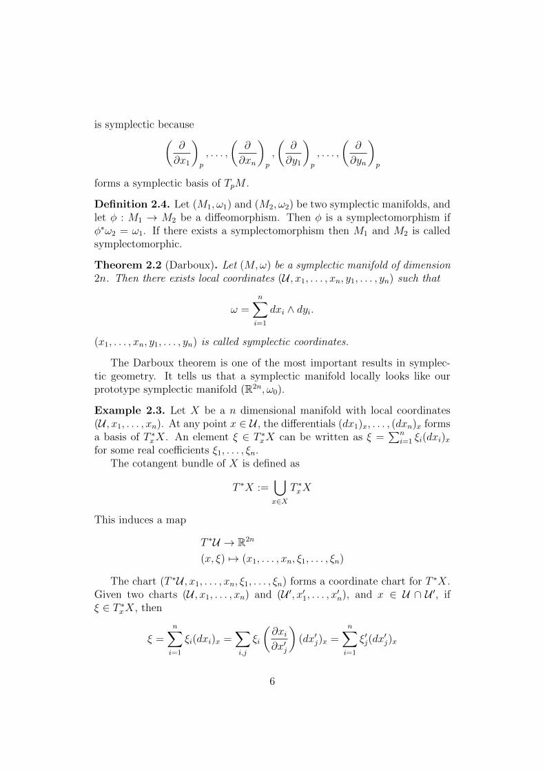
is symplectic because(∂

∂x1

)p

, . . . ,

(∂

∂xn

)p

,

(∂

∂y1

)p

, . . . ,

(∂

∂yn

)p

forms a symplectic basis of TpM .

Definition 2.4. Let (M1, ω1) and (M2, ω2) be two symplectic manifolds, andlet φ : M1 → M2 be a diffeomorphism. Then φ is a symplectomorphism ifφ∗ω2 = ω1. If there exists a symplectomorphism then M1 and M2 is calledsymplectomorphic.

Theorem 2.2 (Darboux). Let (M,ω) be a symplectic manifold of dimension2n. Then there exists local coordinates (U , x1, . . . , xn, y1, . . . , yn) such that

ω =n∑i=1

dxi ∧ dyi.

(x1, . . . , xn, y1, . . . , yn) is called symplectic coordinates.

The Darboux theorem is one of the most important results in symplec-tic geometry. It tells us that a symplectic manifold locally looks like ourprototype symplectic manifold (R2n, ω0).

Example 2.3. Let X be a n dimensional manifold with local coordinates(U , x1, . . . , xn). At any point x ∈ U , the differentials (dx1)x, . . . , (dxn)x formsa basis of T ∗xX. An element ξ ∈ T ∗xX can be written as ξ =

∑ni=1 ξi(dxi)x

for some real coefficients ξ1, . . . , ξn.The cotangent bundle of X is defined as

T ∗X :=⋃x∈X

T ∗xX

This induces a map

T ∗U → R2n

(x, ξ) 7→ (x1, . . . , xn, ξ1, . . . , ξn)

The chart (T ∗U , x1, . . . , xn, ξ1, . . . , ξn) forms a coordinate chart for T ∗X.Given two charts (U , x1, . . . , xn) and (U ′, x′1, . . . , x′n), and x ∈ U ∩ U ′, ifξ ∈ T ∗xX, then

ξ =n∑i=1

ξi(dxi)x =∑i,j

ξi

(∂xi∂x′j

)(dx′j)x =

n∑i=1

ξ′j(dx′j)x

6

where ξ′j =∑

i ξi

(∂xi∂x′j

)is smooth. Hence T ∗X is a 2n dimensional man-

ifold with local coordinates (T ∗U , x1, . . . , xn, ξ1, . . . , ξn).Let

π : T ∗X → X

p = (x, ξ) 7→ x

be the natural projection. The tautological one-form α may be defined point-wise as

αp = (dπp)∗ξ ∈ T ∗p (T ∗X)

where (dπ)∗ is the transpose of dπ, that is, (dπp)∗ξ = ξ dπp. Where the

map

dπp : Tp(T∗X))→ TxX

sends ∂∂xj

to ∂∂xj

and ∂∂ξj

to 0.

We can define the canonical symplectic form on a cotangent bundle in acoordinate-free way as ω = −dα.

In the coordinates (x1, . . . , xn, ξ1, . . . , ξn) the tautological form is on theform

α =n∑i=1

ξidxi.

We can now see that the symplectic ω =∑n

i=1 dxi ∧ dξi = −dα which meansthat (x1, . . . , xn, ξ1, . . . , ξn) are symplectic coordinates on T ∗X.

2.2 Isotopies and vector fields

The concept of a flow on a manifold is of high importance in classical me-chanics, because the state of the system follows the flow of the Hamiltonianvector field.

Definition 2.5. Let M be a manifold, a map ρ : M ×R→M is an isotopyif ρt(p) := ρ(p, t) is a diffeomorphism for all t ∈ R and ρ0(p) = p. Given anisotopy ρ we get a time-dependent vector field vt such that

vt ρt =dρtdt

7

So the time derivative of the isotopy defines the vector field vt, thatmeans that for each ρt we can define a time-dependent vector field. If Mis a compact manifold we have one-to-one correspondence of isotopies andtime-dependent vector fields on M .

Definition 2.6. When v is a time-independent vector field the correspondingisotopy is called the flow or the exponential map of the vector field. It is oftenwritten as ρt = exp tv and it is a smooth family of diffeomorphisms on M .

For a fixed point p ∈M we call the map ρ(p, t) : R→M for the integralcurve through p. The elements of the corresponding vector field at pointsalong the curve is clearly tangent vectors to the curve. We also have thatρt ρs = ρt+s therefore ρt forms an abelian group called the one parametergroup.

Definition 2.7. The Lie derivative by vt is the operator

Lvt : Ωk(M)→ Ωk(M)

defined by

Lvt =d

dt(ρt)

∗ω|t=0

The Lie derivative of a r-form along a vector field tells us something abouthow much the form changes along the flow of the vector field.

Proposition 2.1 (Cartan magic formula). Let ω be a differential form. Fora given time-independent vector field v we find that

Lvω = d ιvω + ιv dω. (1)

We also have that when vt be a time-dependent vector field, then

d

dtρ∗tω = ρ∗tLvtω.

ιv is the interior product with respect to v defined as (ιvω)(X1, X2, ..., Xr−1) =ω(v,X1, ..., Xr−1), the interior product sends r-forms to (r − 1)-forms.

3 Hamiltonian mechanics

3.1 Hamiltonian and symplectic vector fields

For a given smooth function H ∈ C∞(M) on a symplectic manifold (M,ω)we can define a unique vector field XH , called the Hamiltonian vector fieldto the Hamiltonian function H as ιXH

ω = dH.

8

Proposition 3.1. Let ρt be the flow generated by the Hamiltonian vectorfield Xf . Then we can see that the symplectic form is preserved by the oneparameter group, that is ρ∗tω = ω.

Proof.

d

dtρ∗tω = ρ∗tLXf

ω = ρ∗t (d ιXfω + ιXf

dω) = ρ∗td df = 0

⇒ ρ∗tω = const. since ρ∗0ω = ω ⇒ ρ∗tω = ω ∀t ∈ R

Because of this the family of diffeomorphisms ρt generated by a functionis symplectomorphisms on (M,ω).

Definition 3.1. A vector field X on (M,ω) is a symplectic vector field if ωis preserved along the flow generated by X. This happens exactly when ιXωis closed.

It is clear that all Hamiltonian vector fields are symplectic because allexact forms are closed.

3.2 Brackets

Definition 3.2. A Lie algebra is a vector space g with a Lie bracket [·, ·],i.e. a bilinear map

[·, ·] : g× g→ g

such that

[X, Y ] = −[Y,X] ∀X, Y ∈ g

0 = [X, [Y, Z]] + [Z, [X, Y ]] + [Y, [Z,X]] ∀X, Y, Z ∈ g

Definition 3.3. The Lie bracket of a vector field Y along the flow of a vectorfield X is defined as

[X, Y ] := LXY =d

dt(ρ)∗Y |t=0

The set of vector fields on a manifold M with the Lie bracket defined asabove defines a Lie algebra.

Theorem 3.1. Let X and Y be symplectic vector fields on a symplectic man-ifold (M,ω), then [X, Y ] is Hamiltonian with Hamiltonian function ω(X, Y ).

9

Definition 3.4. A Poisson bracket is a Lie bracket that follows Leibniz rule,X, Y Z = X, Y Z + Y X,Z. A manifold M is a Poisson manifold if theset of continuous functions on M , C∞(M) has a Poisson bracket.

On any symplectic manifold (M,ω) we can define a Poisson bracket,

f, g = ιXfιXgω = ω(Xf , Xg) ∀f, g ∈ C∞(M)

where Xf , Xg is the Hamiltonian vector field of the functions f, g. Thisimplies that every symplectic manifold is a Poisson manifold. This Poissonbracket is often called the Poisson bracket.

Theorem 3.2. Let f and g be smooth functions on a symplectic manifold(M,ω) and let exp tXg be the flow generated by g, then

f :=d

dt(f exp tXg) = g, f

Proof.

d

dtf(exp tXg) = exp(tXg)

∗LXgf

= exp(tXg)∗(ιXgdf + dιXgf) = exp(tXg)

∗ιXgdf

= exp(tXg)∗ιXgιXf

ω = exp(tXg)∗f, g ⇒ f, g exp(tXg) = f

3.3 Classical mechanics

We are going to look at the classical phase space as a differentiable manifoldwith a symplectic form. The Hamiltonian function of the system is just afunction on the manifold, and from the corresponding vector field we get outHamilton’s equations. Usually the phase space is a 2n dimensional manifoldM , such that M = T ∗X is the cotangent bundle for some n dimensionalmanifold that often is the configuration space of the system.

In this section we let (M,ω) be a 2n dimensional symplectic manifold withsymplectic coordinates q1, . . . qn, p1 . . . , pn and H the Hamiltonian function ofthe system. The fact that (q, p) are the symplectic coordinates of the systemmeans that ω =

∑ni=1 dqi ∧ dpi. And XH is the Hamiltonian vector field of

H, that is ιXHω = dH.

From section 3.2 we have that

F :=d

dt(F ρt) = H,F

10

That means that the time evolution of a function F along the flow definedby H is defined by the Poisson bracket. We can use this to find Hamilton’sequations. In symplectic coordinates q1, . . . , qn, p1, . . . , pn we have that

ιXHω = dH

We also know that the differential dH is on the form

dH =n∑i=1

(∂H

∂qidqi +

∂H

∂pidpi

)Using theorem 3.2 we also have that

qi = H, qi = ω(XH , Xqi) = ιXqidH

We know that the Hamiltonian vector field corresponding to qi is of theform

Xqi =n∑i=1

(ai∂

∂qi+ bi

∂

∂pi

)which implies

dqi = ιXqiω =

n∑j=1

(ajdp− bjdq)⇒ bi = −1, aj = 0, bj = 0 for i 6= j ⇒ Xqi =∂

∂pi

⇒ qi = ιXqidH =

∂H

∂pi

In the same way we can show that

pi = H, pi = −∂H∂qi

It follows from this that dH =∑n

i=1(qidpi − pidqi).The solution to the differential equations

qi =∂H

∂pi

pi = −∂H∂qi

Hamilton’s equations (2)

is the flow generated by XH . For a given initial point q(0), p(0) thesolution is an integral curve. We also have that the Hamiltonian function isconstant along its flow, that is, it is constant along the solution (q(t), p(t))to equation (2).

11

3.4 Integrable systems

Definition 3.5. A Hamiltonian system is a triple (M,ω,H), where (M,ω)is a symplectic manifold and H is a smooth function on M called the Hamil-tonian function.

Proposition 3.2. We have f,H = 0 if and only if f is constant along theintegral curves of XH .

Proof. It follows from theorem 3.2.

A function f such that f,H = 0 is called an integral of motion. Thefunctions f1, . . . fn are said to be linearly independent if their differentials(df1)p, . . . , (dfn)p are linearly independent at each point p ∈M .

Definition 3.6. A Hamiltonian system (M,ω,H) is integrable if it possessesn = 1

2DimM independent integrals of motion H = H1, H2, . . . , Hn, such that

Hi, Hj = 0 for all i, j.

Lemma 3.1. Let (M,ω,H), be an integrable system of dimension 2n withintegrals of motion H = f1, . . . , fn. Let c ∈ Rn be a regular value of f :=f1, . . . , fn. If the Hamiltonian vector fields Xf1 , . . . , Xfn are complete onthe level f−1(c), then the connected components of f−1(c) are of the formRn−k × Tk for some k, 0 ≤ k ≤ n, where Tk is the k-dimensional torus.

Any compact component f−1(c) must hence be a torus. These compo-nents, when they exist, are called Liouville tori.

Theorem 3.3 (Arnold-Liouville). Let (M,ω,H), be an integrable system ofdimension 2n with integrals of motion f1, . . . , fn, and let c ∈ Rn be a regularvalue of f .

1. If the flows of Xf1 , . . . , Xfn starting at a point p ∈ f−1(c) are complete,then the connected component of f−1(c) containing p is a homogeneousspace for Rn. With respect to this structure, the component have coor-dinates φ1, . . . , φn, known as angle coordinates, in which the flows ofthe vector fields Xf1 , . . . , Xfn are linear.

2. There are coordinates ψ1, . . . , ψn, known as action coordinates, comple-mentary to the angle coordinates such that ψi are integrals of motionand φ1, . . . , ψn, ψ1, . . . , ψn are symplectic coordinates.

12

4 Moment maps

4.1 Lie groups

Definition 4.1. A Lie group is a smooth manifold which also have a groupstructure. That is a smooth manifold G with a group operation · such that

G×G→ G

(g1, g2) 7→ g1 · g2

and

G→ G

g 7→ g−1

are smooth maps. We will denote the identity element of G as e.

Example 4.1. • R with addition

• S1 regarded as unit complex numbers with multiplications, representsrotations of the plane.

• U(n), unitary linear transformations of Cn.

• SU(n), unitary linear transformations of Cn with det = 1.

• O(n), orthogonal linear transformations of Rn.

• SO(n), elements of O(n) with det = 1

• GL(V ), invertible linear transformations of a vector space V .

4.2 Smooth actions

Definition 4.2. An action of a Lie group G on a manifold M is a grouphomomorphism

ψ : M ×G→M

(p, g) 7→ ψg(p).

It is a smooth action if ψ is a smooth map.

13

Example 4.2. Let X be a complete vector field on M and let G = R, then

ρ : M × R→M

(p, t) 7→ ρt(p) = exp(tX)(p)

is a smooth action of R on M . So for each complete vector field on M wehave a smooth R action, in fact it is a one to one correspondence.

Definition 4.3. A group action ψ of a group G on (M,ω) is called a sym-plectic action when all the diffeomorphisms ψg also are symplectomorphisms.

Example 4.3. If G = R then the smooth action ψt = exp tX is symplecticwhen X is a symplectic vector field.

Example 4.4. Let M = R2n, ω =∑dxi ∧ dyi and X = − ∂

∂y1. The orbits of

the action generated by X are lines parallel to the y1-axis,

(x1, y1 − t, x2, y2, . . . , yn)|t ∈ R

4.3 Orbit spaces

Definition 4.4. Let ψ be a action of G on M . The orbit of G through p ∈Mis ψg(p)|g ∈ G.

The Stabilizer of p ∈M is the subgroup Gp := g ∈ G|ψg(p) = p.

Definition 4.5. We say that the action of G on M is respectively:

• transitive if there is just one orbit,

• free if all stabilizers are trivial e.

Let ∼ be the equivalence relation for points in p, q ∈M such that

p ∼ q ⇔ p and q is in the same orbit

Definition 4.6. The quotient space M/G := M/ ∼ is the space of all orbitsof an action on M , we call it the orbit space. If the action is transitive thenM/G is trivial.

14

4.4 Adjoint and coadjoint representation

Let G be a Lie group. Given a ∈ G let

La : G→ G

g 7→ ag.

be left multiplication by a. A vector field X is called left-invariant ifLa∗X|g = X|ag ∀a ∈ G. Let g be the set of left-invariant vector fields on G.

The Lie bracket [X, Y ] is defined as the Lie derivative of Y along the flowof X:

LXY =d

dt(ρ)∗Y |t=0 = [X, Y ]. (3)

g with the Lie bracket [·, ·] forms a Lie algebra, called the Lie algebra ofG.

For every element V ∈ TeG we can associate a unique left-invariant vectorfield XV on G

XV := Lg∗V

and for every left-invariant vector field we get an element in Te(G)

X|e := V

It follows that TeG and g are isomorphic and hence dim(g) = dim(TeG).The set of vector fields on a manifold M with the Lie bracket as in (3) is

also a Lie algebra.Next we define an action of a Lie group G on itself called the adjoint

representation of G. The action is defined as:

ψ : G×G→ G

(a, g) 7→ ψ(a, g) = ada(g) = aga−1.

If we restrict the push-forward map ada∗ : TgG → Tada gG to g = e then weget a map

Ada := ada∗ |TeG : TeG→ TeG

Since TeG is isomorphic to g, Ad : G× g→ g is an action of G on its Liealgebra g called the adjoint map or the adjoint action.

If g∗ is the dual vector space of g we can define the coadjoint action Ad∗.That is

Ad∗ : g∗ ×G→ g∗

15

where Ad∗ is defined as

〈Ad∗g η,X〉 = 〈η,Adg−1 X〉 ∀X ∈ g, η ∈ g∗

Where 〈·, ·〉 is the natural pairing of g with its dual space.

Theorem 4.1. Let G be a matrix group and X, Y ∈ g, then

d

dtAdexp tX Y

∣∣∣∣t=0

= [X, Y ].

4.5 Moment and comoment maps

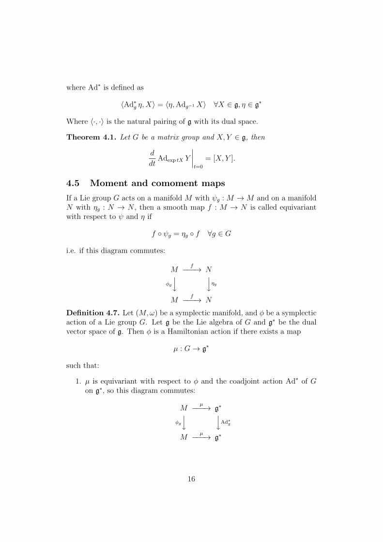
If a Lie group G acts on a manifold M with ψg : M →M and on a manifoldN with ηg : N → N , then a smooth map f : M → N is called equivariantwith respect to ψ and η if

f ψg = ηg f ∀g ∈ G

i.e. if this diagram commutes:

Mf−−−→ N

φg

y yηgM

f−−−→ N

Definition 4.7. Let (M,ω) be a symplectic manifold, and φ be a symplecticaction of a Lie group G. Let g be the Lie algebra of G and g∗ be the dualvector space of g. Then φ is a Hamiltonian action if there exists a map

µ : G→ g∗

such that:

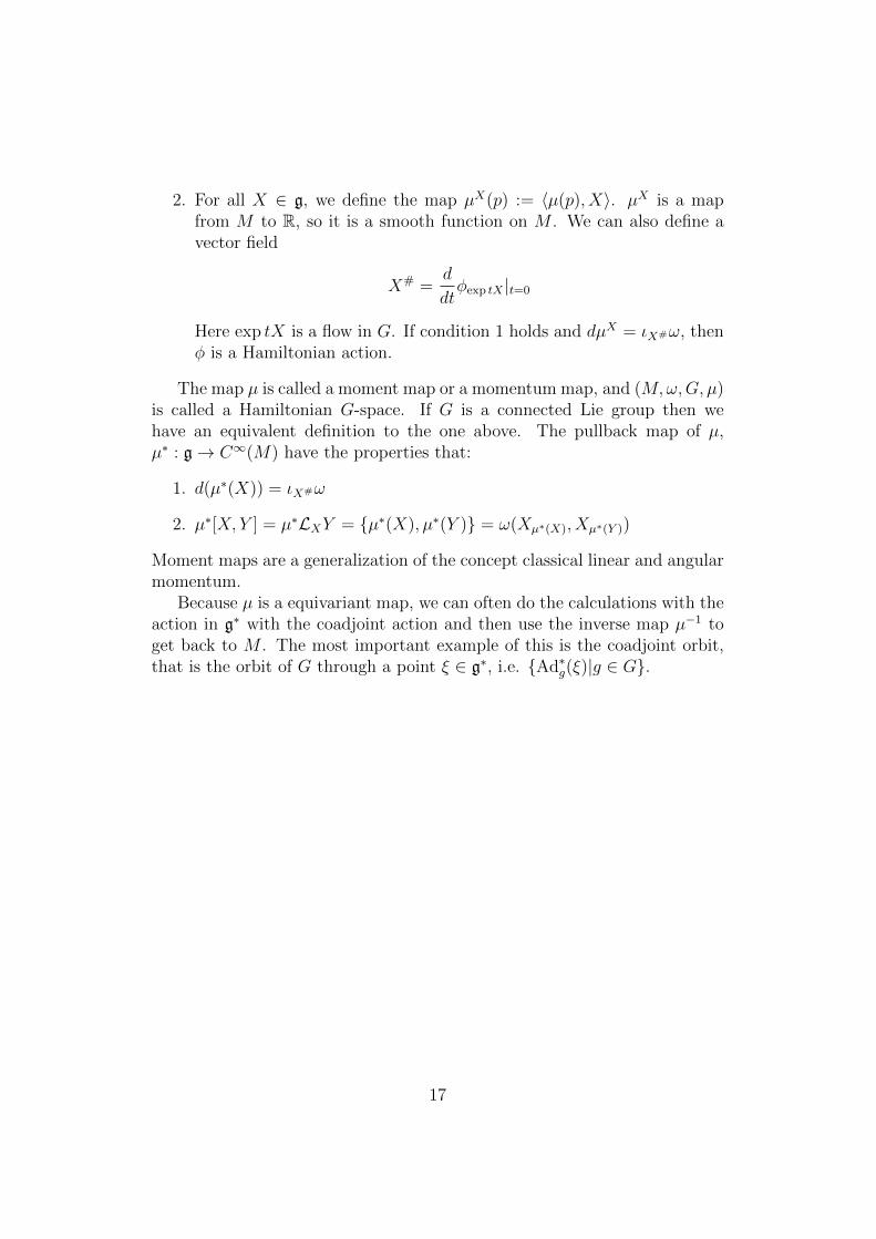
1. µ is equivariant with respect to φ and the coadjoint action Ad∗ of Gon g∗, so this diagram commutes:

Mµ−−−→ g∗

φg

y yAd∗g

Mµ−−−→ g∗

16

2. For all X ∈ g, we define the map µX(p) := 〈µ(p), X〉. µX is a mapfrom M to R, so it is a smooth function on M . We can also define avector field

X# =d

dtφexp tX |t=0

Here exp tX is a flow in G. If condition 1 holds and dµX = ιX#ω, thenφ is a Hamiltonian action.

The map µ is called a moment map or a momentum map, and (M,ω,G, µ)is called a Hamiltonian G-space. If G is a connected Lie group then wehave an equivalent definition to the one above. The pullback map of µ,µ∗ : g→ C∞(M) have the properties that:

1. d(µ∗(X)) = ιX#ω

2. µ∗[X, Y ] = µ∗LXY = µ∗(X), µ∗(Y ) = ω(Xµ∗(X), Xµ∗(Y ))

Moment maps are a generalization of the concept classical linear and angularmomentum.

Because µ is a equivariant map, we can often do the calculations with theaction in g∗ with the coadjoint action and then use the inverse map µ−1 toget back to M . The most important example of this is the coadjoint orbit,that is the orbit of G through a point ξ ∈ g∗, i.e. Ad∗g(ξ)|g ∈ G.

17

5 Symplectic reduction

5.1 Marsden-Weinstein-Meyer theorem

Theorem 5.1 (Marsden-Weinstein-Meyer). Let (M,ω,G, µ) be a Hamilto-nian G-space for a compact Lie group G. Let i : µ−1(0) →M be the inclusionmap.Let π : M → M/G be the point-orbit projection, which sends points toits orbit. Assume that G acts freely on µ−1(0). Then

• the orbit space Mred = µ−1(0)/G is a manifold,

• π : µ−1(0)→Mred is a principal G-bundle, and

• there is a symplectic form ωred on Mred satisfying i∗ω = π∗ωred.

Definition 5.1. The pair (Mred, ωred) is called the reduction or the reducedspace of (M,ω) with respect to G and µ.

The Marsden-Weinstein-Meyer theorem tells us that we can use symme-tries in our system to reduce it to something easier. Again, the proof of thetheorem can be found in [4].

5.2 Noether principle

Theorem 5.2 (Noether). Let (M,ω,G, µ) be a Hamiltonian G-space. Iff : M → R is a G-invariant function, then µ is constant on the trajectoriesof the Hamiltonian vector field of f .

Proof. Let vf be the Hamiltonian vector field of f . Let X ∈ g and µX =〈µ,X〉 : M → R. We have

Lvf = ιvfdµX = ιvf ιX#ω

= −ιX#ιvfω = −ιX#df

= −LX#f = 0

Definition 5.2. A G-invariant function f : M → R is called an integral ofmotion of (M,ω,G, µ). If µ is constant on the trajectories of a Hamiltonianvector field vf , then the corresponding one-parameter group of diffeomor-phisms exp tvf |t ∈ R is called a symmetry of (M,ω,G, µ) .

This means that there is a one-to-one correspondence between symmetriesand integrals of motions for the system.

18

5.3 Elementary theory of reduction

If we find a symmetry for a (2n)-dimensional problem we can reduce it to a(2n−2)-dimensional problem. We are now going to show how we can under-stand the trajectories in a 2n-dimensional system in terms of the trajectoriesof the reduced space.

Example 5.1. Let (M,ω,H) be a Hamiltonian system and let f be anintegral of motion. This implies that f,H = f = 0. Suppose that we canchoose symplectic coordinates

(q1, . . . , qn, p1, . . . pn)

on an open set in M with pn = f .In these coordinates the Hamiltonian is a function of q1, . . . , qn, p1, . . . pn.

Since f is constant along the flow of XH we have that

pn, H = 0 = pn = −∂H∂qn

⇒ H = H(q1, . . . , qn−1, p1, . . . pn).

Since pn is constant we can set it to a fixed value c ∈ R. The motion ofthe system is descibed by the following Hamilton equations:

dqidt

=∂H

∂pi(q1, . . . , qn−1, p1, . . . , pn−1, c) for i = 1, . . . , n− 1

dpidt

= −∂H∂qi

(q1, . . . , qn−1, p1, . . . , pn−1, c) for i = 1, . . . , n− 1

dqndt

=∂H

∂pndpndt

= −∂H∂qn

= 0

The reduced phase space is

Ured = (q1, . . . , qn−1, p1, . . . , pn−1) ∈ R2n−2|(q1, . . . , qn−1, a, p1, . . . , pn−1, c) ∈ U for some a.

The reduced Hamiltonian is

Hred : Ured → RHred(q1, . . . , qn−1, p1, . . . , pn−1) := H(q1, . . . , qn−1, p1, . . . , pn−1, c).

19

We now have a reduced space Mred of dimension 2n − 2 which we need tofind the trajectories in, but for qn(t) and pn(t) we have

qn(t) = qn(0) +

∫ t

0

∂H

∂pndt

pn(t) = c.

If g is a integral of motion independent of f , then we can use g to reducethe phase space to a (2n− 4)-dimensional phase space, and the trajectoriesof qn−1 and pn−1 can be found in the same way as for those of qn and pn.This means that if we have n independent integrals of motion we can find thetrajectories for all of qi and pi, and that is why a system with n independentintegrals of motion is called integrable.

5.4 Reduction at other levels

We are now going to look at reduction along a coadjoint orbit. Let G be acompact Lie group that acts on a symplectic manifold (M,ω) in a Hamil-tonian way with moment map µ : M → g∗. Let ξ ∈ g∗, and let O be thecoadjoint orbit through ξ.

The reduction of M along O is defined as µ−1(O)/G, i.e. it is the set oforbits in µ−1(O) ⊂M generated by the action of G.

Definition 5.3. µ−1(O)/G is called the symplectic reduction of M withrespect to G along O. We denote is by R(M,G,O).

Lemma 5.1. If the action of G on µ−1 is free, then R(M,G,O) is symplecticand dim(R(M,G,O)) = dim(M)− 2 dim(G) + dim(O)

6 Calogero-Moser systems

There are several kinds of Calogero-Moser systems, all of them are one di-mensional problems. The Hamiltonian of Calogero-Moser systems is of theform: ∑

i

p2i +∑i 6=j

U(xi − xj)

Where the potential U can have several forms. The two types of systemswe will look at here is the rational and the trigonometric Calogero-Mosersystems. That is when U = 1

(xi−xj)2 and U = 14 sin2((xi−xj)/2)

respectively.

The trigonometric system is also called Sutherland system. The Sutherland

20

systems might be viewed as N particles on a circle with a inverse square ofthe distance potential. And the rational system corresponds to particles ona line with a 1/d2 potential.

6.1 Calogero-Moser space

In the following sections we have a symplectic manifold M = T ∗Matn(C)1,with symplectic form ω = tr(dY ∧dX) =

∑ni,j=1 dYij ∧dXij. We can identify

M with Matn(C) ⊕Matn(C), so an element in M is just a pair of complexmatrices (X, Y ). Thus dimM = 2n2.

Example 6.1. • GLn(C) = M ∈ Matn(C) | detM 6= 0GLn(C) is called the general linear group and it have dimension n2.

• SLn(C) = M ∈ Matn(C) | detM = 1SLn(C) is called the special linear group and it have dimension n2 − 1.

• PGLn(C)) := GLn(C)/ ∼PGLn(C) is the projective general linear group. ∼ is the equivalencerelation such that A ∼ αA for α ∈ C, i.e. we identify matrices that areequal up to multiplication by a non zero complex number.

We can relate PGLn(C) to SLn(C) 2by using the fact that two matricesA and λA in PGLn(C) is equal. This means that we can choose λ suchthat

detλA = 1.

So we have a one-to-one correspondence between elements in PGLn(C)and SLn(C). That means that dim PGLn(C) = dim SLn(C) = n2 − 1.

Let the projective general linear group G = PGLn(C) act on M with theaction

ψg(X, Y ) := (g−1Xg, g−1Y g)

for g ∈ PGLn(C). The Lie algebra of PGLn(C) is sln(C). The dual space ofsln(C) is of course also sln(C).

1In this section all manifolds will be complex manifolds, rather than real manifoldswhich we used in the previous sections, and also symplectic forms are going to be holo-morphic symplectic forms.

2We are later going to use this to show that the Lie algebra of PGLn(C) is sln(C).

21

The Lie algebra sln(C) is defined as the set of traceless n × n matrices,with the commutator [X, Y ] = XY − Y X as its Lie bracket. We identifyelements in the dual space by using the trace form.

We define a map

µ : M → g∗ = sln(C)

(X, Y ) 7→ [X, Y ] = XY − Y X

We are now going to show that the action of G on M is a Hamiltonianaction with respect to µ. So we have to show that µ is a moment map.

• We need to show that µ is a equivariant with respect to the actionψg : M → M of G, where ψg(X, Y ) = (g−1Xg, g−1Y g). That is weneed to show that µ ψg = Ad∗g µ. We have that

(Ad∗g µ)(X, Y ) = Ad∗g([X, Y ]) = g−1[X, Y ]g

On the other hand we have

(µ ψg)(X, Y ) = µ(g−1Xg, g−1Y g) = g−1Xgg−1Y g − g−1Y gg−1Xg= g−1[X, Y ]g.

So we are done.

• For ξ ∈ g, we define µξ(X, Y ) = 〈µ(X, Y ), ξ〉 = tr([X, Y ]ξ) = tr(X[Y, ξ]).We need to show that dµξ = ιξ#ω Using Cartan magic formula, andthe Tautological one-form ω = dα we can simplify our condition to

dµξ = ιξ#ω = ιξ#dα = Lξ#α− dιξ#α = −dιξ#α.

This means that we have to show that tr([X, Y ]ξ) = −ιξ#α. We havethat

ξ#(X, Y ) =d

dt(ψexp tξ(X, Y )) =

d

dt(Adexp−tξX,Adexp−tξ Y ) = ([X, ξ], [Y, ξ])

We also have that

α = tr(Y dX)

Using this we find that

−ιξ#α = −ιξ# trY dX = − tr(Y [X, ξ]) = tr([X, Y ]ξ)

22

We have now shown that ψ is a Hamiltonian action with the moment mapµ.

Example 6.2. µ−1(0) is the subspace of M such that the pair of matrices(X, Y ) commutes. The reduced space Mred = µ−1(0)/G is the set of G-orbitson µ−1(0) as usual.

Definition 6.1. The Calogero-Moser space is defined as the reduced spacealong the coadjoint orbitO that goes through the point γ := diag(−1,−1, . . . , n−1) ∈ sln(C). The Calogero-Moser space is denoted Cn := R(M,G,O), and isthe set of orbits of the action of PGLn(C) on µ−1(O) ⊂ T ∗Matn(C).

Lemma 6.1. The orbit O = g−1γg|g ∈ PGLn(C) = T ∈ sln(C)| rank(T+1) = 1 is the set of traceless matrices T such that T + 1 has rank one.

Proof.

tr(g−1γg) = tr γ = 0

rank(g−1γg + 1) = rank(g−1γg + g−11g) = rank(g−1(γ + 1)g) = rank(γ + 1) = 1

µ−1(O) is the pair of matrices (X, Y ) such that rank(µ(X, Y ) + 1) =rank([X, Y ] + 1) = 1.

Using lemma 5.1 we can show that dim Cn = 2n. We already know thedimension of M and G, so we only need to find the dimension of O.

Let T ∈ O. We know that a matrix with rank one can be written on theform

a1b1 a1b2 · · · a1bna2b1 a2b2 · · · a2bn

......

. . ....

anb1 anb2 · · · anbn

.

Since T + 1 has rank one we have that

T =

a1b1 − 1 a1b2 · · · a1bna2b1 a2b2 − 1 · · · a2bn

......

. . ....

anb1 anb2 · · · anbn − 1

23

We also have two constraint on T , that is

trT = 0

and the gauge degree of freedom a 7→ λa, b 7→ b/λ. Using this we see that

dimO = 2n− 2

dim Cn = dim(M)− 2 dim(G) + dim(O) = 2n2 − 2(n2 − 1) + 2n− 2 = 2n

6.2 Rational Calogero-Moser system

We start this section by defining n functions Hi = tr(Y i) on M . Hi, Hj = 0because Hi does not depend on X. Since Hi = tr(Y i) then we have thatdHi =

∑ni,j=1 aijdyij for some aij and where yij is the elements of Y . The

Hamiltonian vector field will be of the form XHi=∑n

i,j=1

(bij

∂∂yij

+ cij∂

∂xij

).

We use the interior product ιXHiω =

∑ni,j=1 (bijdxij + cijdyij) to show that

bij = 0 and aij = cij since ιHiω = dHi. So the Hamiltonian vector fields for

the functions Hi is of the form∑n

i,j=1 aij∂

∂xij. This implies that

Hi, Hj = ιHjιHiω = ιHj

dHi =n∑

i,j=1

aijdyij

(n∑

i,j=1

aij∂

∂xij

)= 0

Since dim(Cn) = 2n our functions Hi are an integrable system on Cn. Therational Calogero-Moser system is the phase space Cn with the HamiltonianH2 = tr(Y 2). Since H2 is included in the the integrable system H1, . . . Hn

we know that the rational Calogero-Moser system is integrable. We will nowshow how to find a solution to this system, and show why it is the same asthe system of n particles on a line.

Theorem 6.1. We are now going to introduce a theorem called the Necklacebracket formula. It says that if a1, . . . , ar, b1, . . . , bs is either X or Y . Thenwe have

tr(a1 · a2 · · · ar), tr(b1 · · · bs) =∑(i,j)

ai=Y,bj=X

tr(ai+1 · · · ara1 · · · ai−1bj+1 · · · bsb1 · · · aj−1)

−∑(i,j)

ai=X,bj=Y

tr(ai+1 · · · ara1 · · · ai−1bj+1 · · · bsb1 · · · aj−1).

24

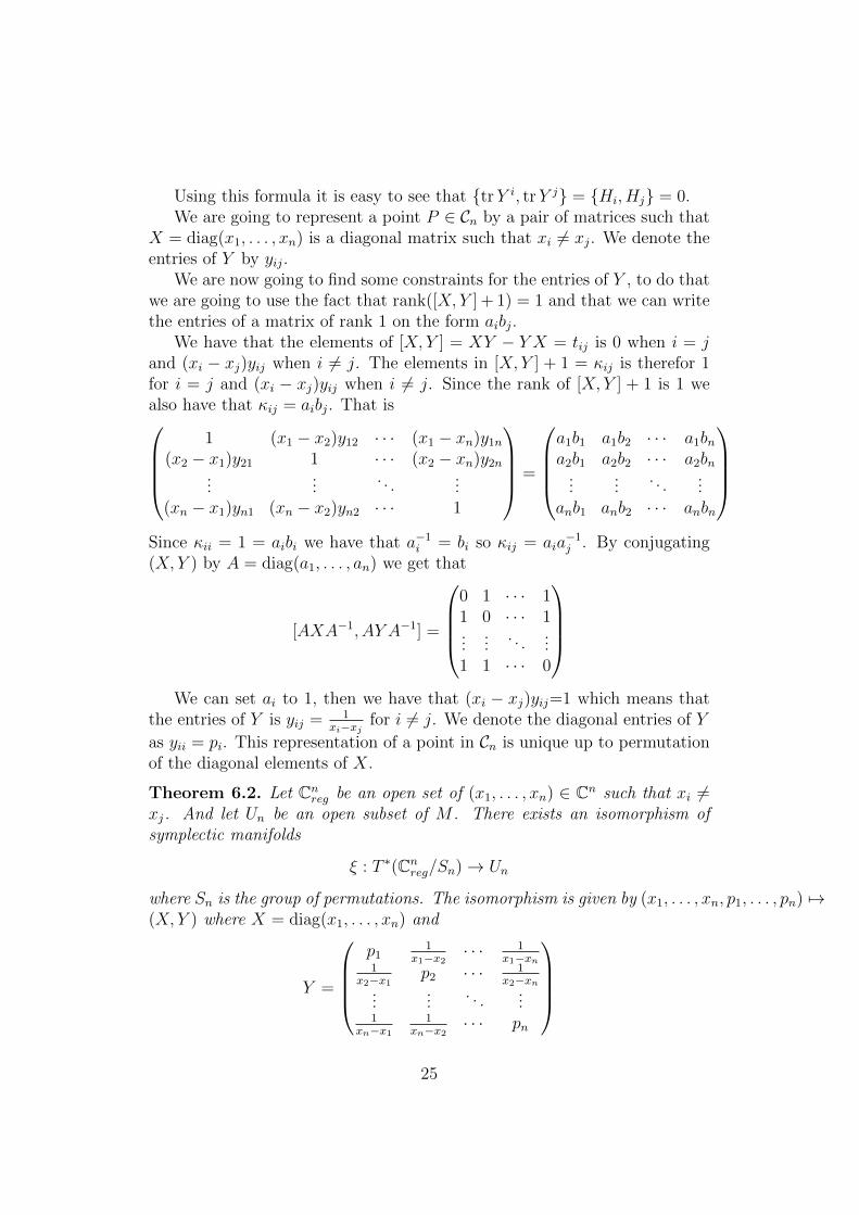
Using this formula it is easy to see that trY i, trY j = Hi, Hj = 0.We are going to represent a point P ∈ Cn by a pair of matrices such that

X = diag(x1, . . . , xn) is a diagonal matrix such that xi 6= xj. We denote theentries of Y by yij.

We are now going to find some constraints for the entries of Y , to do thatwe are going to use the fact that rank([X, Y ] + 1) = 1 and that we can writethe entries of a matrix of rank 1 on the form aibj.

We have that the elements of [X, Y ] = XY − Y X = tij is 0 when i = jand (xi − xj)yij when i 6= j. The elements in [X, Y ] + 1 = κij is therefor 1for i = j and (xi − xj)yij when i 6= j. Since the rank of [X, Y ] + 1 is 1 wealso have that κij = aibj. That is

1 (x1 − x2)y12 · · · (x1 − xn)y1n(x2 − x1)y21 1 · · · (x2 − xn)y2n

......

. . ....

(xn − x1)yn1 (xn − x2)yn2 · · · 1

=

a1b1 a1b2 · · · a1bna2b1 a2b2 · · · a2bn

......

. . ....

anb1 anb2 · · · anbn

Since κii = 1 = aibi we have that a−1i = bi so κij = aia

−1j . By conjugating

(X, Y ) by A = diag(a1, . . . , an) we get that

[AXA−1, AY A−1] =

0 1 · · · 11 0 · · · 1...

.... . .

...1 1 · · · 0

We can set ai to 1, then we have that (xi − xj)yij=1 which means that

the entries of Y is yij = 1xi−xj for i 6= j. We denote the diagonal entries of Y

as yii = pi. This representation of a point in Cn is unique up to permutationof the diagonal elements of X.

Theorem 6.2. Let Cnreg be an open set of (x1, . . . , xn) ∈ Cn such that xi 6=

xj. And let Un be an open subset of M . There exists an isomorphism ofsymplectic manifolds

ξ : T ∗(Cnreg/Sn)→ Un

where Sn is the group of permutations. The isomorphism is given by (x1, . . . , xn, p1, . . . , pn) 7→(X, Y ) where X = diag(x1, . . . , xn) and

Y =

p1

1x1−x2 · · · 1

x1−xn1

x2−x1 p2 · · · 1x2−xn

......

. . ....

1xn−x1

1xn−x2 · · · pn

25

Proof. Let ak = trXk and bk = trXkY . We can use the necklace bracketformula to show that we have

am, ak = 0, bm, ak = kam+k−1, bm, bk = (k −m)bm+k−1.

On the other hand, ξ∗ak =∑xki , ξ

∗bk =∑xki pi. Thus we see that

f, g = ξ∗f, ξ∗g

where f ,g is either ak or bk. Since ak, bk form a local coordinate system neara generic point of Un we are done.

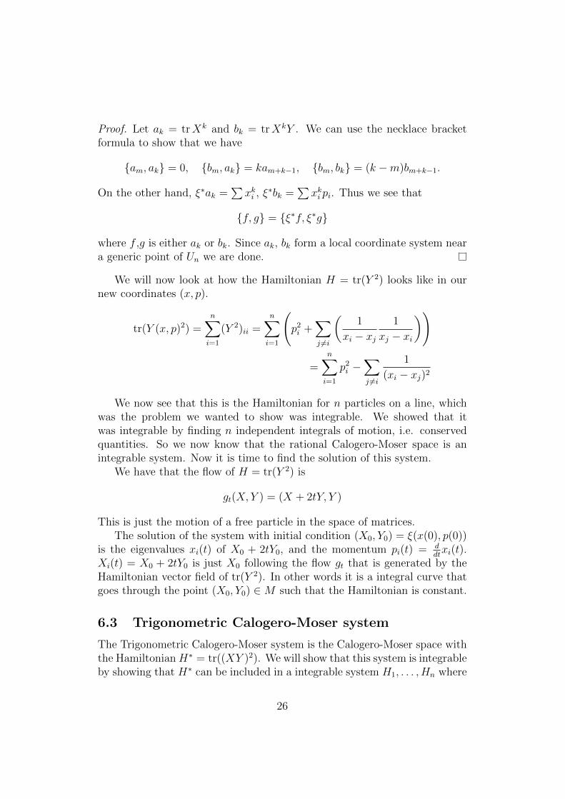
We will now look at how the Hamiltonian H = tr(Y 2) looks like in ournew coordinates (x, p).

tr(Y (x, p)2) =n∑i=1

(Y 2)ii =n∑i=1

(p2i +

∑j 6=i

(1

xi − xj1

xj − xi

))

=n∑i=1

p2i −∑j 6=i

1

(xi − xj)2

We now see that this is the Hamiltonian for n particles on a line, whichwas the problem we wanted to show was integrable. We showed that itwas integrable by finding n independent integrals of motion, i.e. conservedquantities. So we now know that the rational Calogero-Moser space is anintegrable system. Now it is time to find the solution of this system.

We have that the flow of H = tr(Y 2) is

gt(X, Y ) = (X + 2tY, Y )

This is just the motion of a free particle in the space of matrices.The solution of the system with initial condition (X0, Y0) = ξ(x(0), p(0))

is the eigenvalues xi(t) of X0 + 2tY0, and the momentum pi(t) = ddtxi(t).

Xi(t) = X0 + 2tY0 is just X0 following the flow gt that is generated by theHamiltonian vector field of tr(Y 2). In other words it is a integral curve thatgoes through the point (X0, Y0) ∈M such that the Hamiltonian is constant.

6.3 Trigonometric Calogero-Moser system

The Trigonometric Calogero-Moser system is the Calogero-Moser space withthe Hamiltonian H∗ = tr((XY )2). We will show that this system is integrableby showing that H∗ can be included in a integrable system H1, . . . , Hn where

26

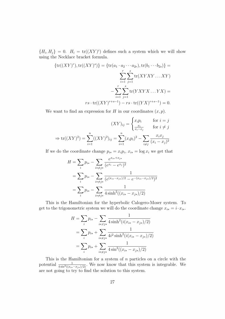
Hi, Hj = 0. Hi = tr((XY )i) defines such a system which we will showusing the Necklace bracket formula.

tr((XY )r), tr((XY )s) = tr(a1 · a2 · · · a2r), tr(b1 · · · b2s) =r∑i=1

s∑j=1

tr(XYXY . . .XY )

−r∑i=1

s∑j=1

tr(Y XY X . . . Y X) =

rs · tr((XY )r+s−1)− rs · tr((Y X)r+s−1) = 0.

We want to find an expression for H in our coordinates (x, p).

(XY )ij =

xipi for i = jxi

xi−xj for i 6= j

⇒ tr((XY )2) =n∑i=1

((XY )2)ij =n∑i=1

(xipi)2 −

∑i 6=j

xixj(xi − xj)2

If we do the coordinate change pi∗ = xipi, xi∗ = log xi we get that

H =∑i

pi∗ −∑i∗6=j∗

exi∗+xj∗

(exi − exj)2

=∑i

pi∗ −∑i∗6=j∗

1

(e(xi∗−xj∗)/2 − e−(xi∗−xj∗)/2)2

=∑i

pi∗ −∑i∗6=j∗

1

4 sinh2((xi∗ − xj∗)/2)

This is the Hamiltonian for the hyperbolic Calogero-Moser system. Toget to the trigonometric system we will do the coordinate change xi∗ = i ·xi∗.

H =∑i

pi∗ −∑i∗6=j∗

1

4 sinh2(i(xi∗ − xj∗)/2)

=∑i

pi∗ +∑i∗6=j∗

1

4i2 sinh2(i(xi∗ − xj∗)/2)

=∑i

pi∗ +∑i∗6=j∗

1

4 sin2((xi∗ − xj∗)/2)

This is the Hamiltonian for a system of n particles on a circle with thepotential 1

4 sin2((xi∗−xj∗)/2). We now know that this system is integrable. We

are not going to try to find the solution to this system.

27

The rational, hyperbolic and trigonometric Calogero-Moser systems areall just special cases of a more general system called the elliptic Calogero-Moser system.

7 Conclusions

In this thesis we showed the integrability for the rational and trigonometricCalogero-Moser systems. That is the Hamiltonian systems with with Hamil-tonian H =

∑ni=1 p

2i −

∑j 6=i

1(xi−xj)2 and H =

∑i pi +

∑i 6=j

14 sin2((xi−xj)/2)

re-

spectively. We did this using symplectic reduction. More specifically we actedsmoothly on the cotangent bundle of n×n complex matrices T ∗Matn(C) withthe Lie group PGLn(C) and defined the Calogero-Moser space as the reducedspace Cn := R(M,G,O). That is the symplectic reduction of T ∗Matn(C)with respect to PGLn(C) along the coadjoint orbit O, where O is the orbitthrough the point diag(−1,−1, . . . , n− 1) ∈ sln(C).

We then look at the Calogero-Moser space as the phase space with sym-plectic form ω = tr(dX ∧ dY ) and a we show that a point in Cn can berepresented as a pair of complex n×n matrices (X, Y ) such that rank(XY −Y X + 1) = 1. We first look at the Hamiltonian system (Cn, ω,H = trY 2)and show that this is an integrable system with integral of motion trY i fori = 1, . . . , n. Then we can do a change of coordinates such that we can seethat this is just the rational Calogero-Moser system.

Then we looked at the Hamiltonian system (Cn, ω,H = tr((XY )2)) andshow that it is integrable with integrals of motion tr((XY )i). We can thensee that this is the trigonometric Calogero-Moser system which is what wewanted.

For future work one might consider to look at the elliptic Calogero-Mosersystem where the rational and trigonometric systems are just special limits.An other alternative is to go to the quantum mechanical case for which therational system first was solved.

References

[1] P.I. Etingof Calogero-Moser systems and representation theory 2007, Eu-ropean Mathematical Society, Zurich

[2] J.E Marsden, T.S. Ratiu Introduction to mechanics and symmetry: abasic exposition of classical mechanical systems 1994, Springer, New York;Berlin

28

[3] M. Nakahara Geometry, topology, and physics 2003, Institute of Physics,Bristol

[4] A. C. d. Silva Lectures on Symplectic Geometry 2001, Springer, New York;Berlin

[5] F. Calogero Solution of the One-Dimensional N-Body Problems withQuadratic and/or Inversely Quadratic Pair Potentials 1971, Journal ofMathematical Physics, vol. 12, no. 3, pp. 419-436.

[6] J. Moser Three Integrable Hamiltonian Systems Connected with Isospec-tral Deformations 1975, Advances in Mathematics, vol. 16, no. 2, pp.197-220.

[7] D. Kazhdan, B.Kostant, S. Sternberg Hamiltonian Group Actions andDynamical Systems of Calogero Type 1978, Communications on Pure andApplied Mathematics, vol. 31, no. 4, pp. 481-507.

29