![Fault-tolerant quantum computation by anyons · noli and M. Rasetti [14], but the question of fault-tolerance was not considered. 1 Toric codes and the corresponding Hamiltonians](https://static.fdocuments.us/doc/165x107/5e634909ec0f2070c52e8b43/fault-tolerant-quantum-computation-by-anyons-noli-and-m-rasetti-14-but-the-question.jpg)
Lecture Notes for Physics 219: Quantum...
68
Lecture Notes for Physics 219: Quantum Computation John Preskill California Institute of Technology 14 June 2004
Transcript of Lecture Notes for Physics 219: Quantum...
Lecture Notes for Physics 219:
Quantum Computation
John Preskill
California Institute of Technology
14 June 2004
Contents
9 Topological quantum computation 4
9.1 Anyons, anyone? 49.2 Flux-charge composites 79.3 Spin and statistics 99.4 Combining anyons 119.5 Unitary representations of the braid group 139.6 Topological degeneracy 169.7 Toric code revisited 209.8 The nonabelian Aharonov-Bohm effect 219.9 Braiding of nonabelian fluxons 249.10 Superselection sectors of a nonabelian superconductor 299.11 Quantum computing with nonabelian fluxons 329.12 Anyon models generalized 40
9.12.1Labels 409.12.2Fusion spaces 419.12.3Braiding: the R-matrix 449.12.4Associativity of fusion: the F -matrix 459.12.5Many anyons: the standard basis 469.12.6Braiding in the standard basis: the B-matrix 47
9.13 Simulating anyons with a quantum circuit 499.14 Fibonacci anyons 529.15 Quantum dimension 539.16 Pentagon and hexagon equations 589.17 Simulating a quantum circuit with Fibonacci anyons 619.18 Epilogue 63
9.18.1Chern-Simons theory 639.18.2S-matrix 649.18.3Edge excitations 65
9.19 Bibliographical notes 65
2
Contents 3
References 67
9Topological quantum computation
9.1 Anyons, anyone?
A central theme of quantum theory is the concept of indistinguishable
particles (also called identical particles). For example, all electrons in theworld are exactly alike. Therefore, for a system with many electrons,an operation that exchanges two of the electrons (swaps their positions)is a symmetry — it leaves the physics unchanged. This symmetry isrepresented by a unitary transformation acting on the many-electron wavefunction.
For the indistinguishable particles in three-dimensional space that wenormally talk about in physics, particle exchanges are represented in oneof two distinct ways. If the particles are bosons (like, for example, 4Heatoms in a superfluid), then an exchange of two particles is represented bythe identity operator: the wave function is invariant, and we say the par-ticles obey Bose statistics. If the particles are fermions (like, for example,electrons in a metal), than an exchange is represented by multiplicationby (−1): the wave function changes sign, and we say that the particlesobey Fermi statistics.
The concept of identical-particle statistics becomes ambiguous in onespatial dimension. The reason is that for two particles to swap positionsin one dimension, the particles need to pass through one another. If thewave function changes sign when two identical particles are exchanged,we could say that the particles are noninteracting fermions, but we couldjust as well say that the particles are interacting bosons, such that thesign change is induced by the interaction as the particles pass one an-other. More generally, the exchange could modify the wavefunction bya multiplicative phase eiθ that could take values other than +1 or −1,but we could account for this phase change by describing the particles aseither bosons or fermions.
4
9.1 Anyons, anyone? 5
Thus, identical-particle statistics is a rather tame concept in three (ormore) spatial dimensions and also in one dimension. But in between thesetwo dull cases, in two dimensions, a remarkably rich variety of types ofparticle statistics are possible, so rich that we have far to go before wecan give a useful classification of all of the possibilities.
Indistinguishable particles in two dimensions that are neither bosonsnor fermions are called anyons. Anyons are a fascinating theoretical con-struct, but do they have anything to do with the physics of real systemsthat can be studied in the laboratory? The remarkable answer is: “Yes!”Even in our three-dimensional world, a two-dimensional gas of electronscan be realized by trapping the electrons in a thin layer between two slabsof semiconductor, so that at low energies, electron motion in the directionorthogonal to the layer is frozen out. In a sufficiently strong magnetic fieldand at sufficiently low temperature, and if the electrons in the materialare sufficiently mobile, the two-dimensional electron gas attains a pro-foundly entangled ground state that is separated from all excited statesby a nonzero energy gap. Furthermore, the low-energy particle excitationsin the systems do not have the quantum numbers of electrons; rather theyare anyons, and carry electric charges that are fractions of the electroncharge. The anyons have spectacular effects on the transport propertiesof the sample, manifested as the fractional quantum Hall effect.
Anyons will be our next topic. But why? True, I have already saidenough to justify that anyons are a deep and fascinating subject. But thisis not a course about the unusual behavior of exotic phases attainable incondensed matter systems. It is a course about quantum computation.
In fact, there is a connection, first appreciated by Alexei Kitaev in1997: anyons provide an unusual, exciting, and perhaps promising meansof realizing fault-tolerant quantum computation.
So that sounds like something we should be interested in. After all,I have already given 12 lectures on the theory of quantum error correc-tion and fault-tolerant quantum computing. It is a beautiful theory; Ihave enjoyed telling you about it and I hope you enjoyed hearing aboutit. But it is also daunting. We’ve seen that an ideal quantum circuitcan be simulated faithfully by a circuit with noisy gates, provided thenoisy gates are not too noisy, and we’ve seen that the overhead in cir-cuit size and depth required for the simulation to succeed is reasonable.These observations greatly boost our confidence that large scale quantumcomputers will really be built and operated someday. Still, for fault tol-erance to be effective, quantum gates need to have quite high fidelity (bythe current standards of experimental physics), and the overhead cost ofachieving fault tolerance is substantial. Even though reliable quantumcomputation with noisy gates is possible in principle, there always will
6 9 Topological quantum computation
be a strong incentive to improve the fidelity of our computation by im-proving the hardware rather than by compensating for the deficiencies ofthe hardware through clever circuit design. By using anyons, we mightachieve fault tolerance by designing hardware with an intrinsic resistanceto decoherence and other errors, significantly reducing the size and depthblowups of our circuit simulations. Clearly, then, we have ample motiva-tion for learning about anyons. Besides, it will be fun!
In some circles, this subject has a reputation (not fully deserved in myview) for being abstruse and inaccessible. I intend to start with the basics,and not to clutter the discussion with details that are mainly irrelevant toour central goals. That way, I hope to keep the presentation clear withoutreally dumbing it down.
What are these goals? I will not be explaining how the theory of anyonsconnects with observed phenomena in fractional quantum Hall systems.In particular, abelian anyons arise in most of these applications. Froma quantum information viewpoint, abelian anyons are relevant to robuststorage of quantum information (and we have already gotten a whiff ofthat connection in our study of toric quantum codes). We will discussabelian anyons here, but our main interest will be in nonabelian anyons,which as we will see can be endowed with surprising computational power.
Kitaev (quant-ph/9707021) pointed out that a system of nonabeliananyons with suitable properties can efficiently simulate a quantum circuit;this idea was elaborated by Ogburn and me (quant-ph/9712048), and gen-eralized by Mochon (quant-ph/0206128, quant-ph/0306063). In Kitaev’soriginal scheme, measurements were required to simulate some quantumgates. Freedman, Larsen and Wang (quant-ph/000110) observed that ifwe use the right kind of anyons, all measurements can be postponed untilthe readout of the final result of the computation. Freedman, Kitaev,and Wang (quant-ph/0001071) also showed that a system of anyons canbe simulated efficiently by a quantum circuit; thus the anyon quantumcomputer and the quantum circuit model have equivalent computationalpower. The aim of these lectures is to explain these important results.
We will focus on the applications of anyons to quantum computing, noton the equally important issue of how systems of anyons with desirableproperties can be realized in practice.∗ It will be left to you to figure thatout!
∗ Two interesting approaches to realizing nonabelian anyons — using superconduct-ing junction arrays and using cold atoms trapped in optical lattices — have beendiscussed in the recent literature.
9.2 Flux-charge composites 7
9.2 Flux-charge composites
For those of us who are put off by abstract mathematical constructions, itwill be helpful to begin our exploration of the theory of anyons by thinkingabout a concrete model. So let’s start by recalling a more familiar concept,the Aharonov-Bohm effect.
Imagine electromagnetism in a two-dimensional world, where a “fluxtube” is a localized “pointlike” object (in three dimensions, you may en-vision a plane intersecting a magnetic solenoid directed perpendicular tothe plane). The flux might be enclosed behind an impenetrable wall, sothat an object outside can never visit the region where the magnetic fieldis nonzero. But even so, the magnetic field has a measurable influence oncharged particles outside the flux tube. If an electric charge q is adiabat-ically transported (counterclockwise) around a flux Φ, the wave functionof the charge acquires a topological phase eiqΦ (where we use units withh = c = 1). Here the word “topological” means that the Aharonov-Bohmphase is robust when we deform the trajectory of the charged particle —all that matters is the “winding number” of the charge about the flux.
The concept of topological invariance arises naturally in the study offault tolerance. Topological properties are those that remain invariantwhen we smoothly deform a system, and a fault-tolerant quantum gate isone whose action on protected information remains invariant (or nearlyso) when we deform the implementation of the gate by adding noise. Thetopological invariance of the Aharonov-Bohm phenomenon is the essentialproperty that we hope to exploit in the design of quantum gates that areintrinsically robust.
We usually regard the Aharonov-Bohm effect as a phenomenon thatoccurs in quantum electrodynamics, where the photon is exactly mass-less. But it is useful to recognize that Aharonov-Bohm phenomena canalso occur in massive theories. For example, we might consider a “super-conducting” system composed of charge e particles, such that compositeobjects with charge ne form a condensate (where n is an integer). Inthis superconductor, there is a quantum of flux Φ0 = 2π/ne, the minimalnonzero flux such that a charge-(ne) particle in the condensate, whentransported around the flux, acquires a trivial Aharonov-Bohm phase.An isolated region that contains a flux quantum is an island of normalmaterial surrounded by the superconducting condensate, prevented fromspreading because the magnetic flux cannot penetrate into the supercon-ductor. That is, it is a stable particle, what we could call a “fluxon.”When one of the charge-e particles is transported around a fluxon, itswave function acquires the nontrivial topological phase eieΦ0 = e2πi/n.But in the superconductor, the photon acquires a mass via the Higgsmechanism, and there are no massless particles. That topological phases
8 9 Topological quantum computation
are compatible with massive theories is important, because massless par-ticles are easily excited, a potentially copious source of decoherence.
Now, let’s imagine that, in our two-dimensional world, flux and electriccharge are permanently bound together (for some reason). A fluxon canbe envisioned as flux Φ confined inside an impenetrable circular wall,and an electric charge q is stuck to the outside of the wall. What isthe angular momentum of this flux-charge composite? Suppose that wecarefully rotate the object counterclockwise by angle 2π, returning it toits original orientation. In doing so, we have transported the charge qabout the flux Φ, generating a topological phase eiqΦ. This rotation by2π is represented in Hilbert space by the unitary transformation
U (2π) = e−i2πJ = eiqΦ , (9.1)
where J is the angular momentum. We conclude, then, that the possibleeigenvalues of angular momentum are
J = m− qΦ
2π(m = integer) . (9.2)
We can characterize this spectrum by an angular variable θ ∈ [0, 2π),defined by θ = qΦ (mod 2π), and say that the eigenvalues are shiftedaway from integer values by −θ/2π. We will refer to the phase eiθ thatrepresents a counterclockwise rotation by 2π as the topological spin of thecomposite object.
But shouldn’t a rotation by 2π act trivially on a physical system (isn’tit the same as doing nothing)? No, we know better than that, from ourexperience with spinors in three dimensions. For a system with fermionnumber F , we have
e−2πiJ = (−1)F ; (9.3)
if the fermion number is odd, the eigenvalues of J are shifted by 1/2from the integers. This shift is physically acceptable because there is a(−1)F superselection rule: no observable local operator can change thevalue of (−1)F (there is no physical process that can create or destroyan isolated fermion). Acting on a coherent superposition of states withdifferent values of (−1)F , the effect of e−2πiJ is
e−i2πJ (a| even F 〉 + b| odd F 〉) = a| even F 〉 − b| odd F 〉 . (9.4)
The relative sign in the superposition flips, but this has no detectablephysical effects, since all observables are block diagonal in the (−1)F
basis.Similarly, in two dimensions, the shift in the angular momentum spec-
trum e−2πiJ = eiθ has no unacceptable physical consequences if there is
9.3 Spin and statistics 9
a θ superselection rule, ensuring that the relative phase in a superposi-tion of states with different values of θ is physically inaccessible (not justin practice but even in principle). As for fermions, there is no allowedphysical process that can create of destroy an isolated anyon.
In three dimensions, only θ = 0, π are allowed, because (as you probablyknow) of a topological property of the three-dimensional rotation groupSO(3): a closed path in SO(3) beginning at the identity and ending at arotation by 4π can be smoothly contracted to a trivial path. It followsthat a rotation by 4π really is represented by the identity, and thereforethat the eigenvalues of a rotation by 2π are +1 and −1. But the two-dimensional rotation group SO(2) does not have this topological property,so that any value of θ is possible in principle.
Note that the angular momentum J changes sign under time reversal(T ) and also under parity (P ). Unless θ = 0 or π, the spectrum of J
is asymmetric about zero, and therefore a theory of anyons typically willnot be T or P invariant. In our flux-charge composite model the originof this symmetry breaking is not mysterious — it arises from the nonzeromagnetic field. But in a system with no intrinsic breaking of T and P , ifanyons occur then either these symmetries must be broken spontaneously,or else the particle spectrum must be “doubled” so that for each anyonwith exchange phase eiθ there also exists an otherwise identical particlewith exchange phase e−iθ.
9.3 Spin and statistics
For identical particles in three dimensions, there is a well known connec-tion between spin and statistics: indistinguishable particles with integerspin are bosons, and those with half-odd-integer spin are fermions. Intwo dimensions, the spin can be any real number. What does this newpossibility of “fractional spin” imply about statistics? The answer is thatstatistics, too, can be “fractionalized”!
What happens if we perform an exchange of two of our flux-chargecomposite objects, in a counterclockwise sense? Each charge q is adiabat-ically transported half way around the flux Φ of the other object. We cananticipate, then, that each charge will acquire an Aharonov-Bohm phasethat is half of the phase generated by a complete revolution of the chargeabout the flux. Adding together the phases arising from the transport ofboth charges, we find that the exchange of the two flux-charge compositeschanges their wave function by the phase
exp
[
i
(
1
2qΦ +
1
2qΦ
)]
= eiqΦ = eiθ = e−2πiJ . (9.5)
The phase generated when the two objects are exchanged matches the
10 9 Topological quantum computation
phase generated when one of the two objects is rotated by 2π. Thus theconnection between spin and statistics continues to hold, in a form thatis a natural generalization of the connection that applies to bosons andfermions.
The origin of this connection is fairly clear in our flux-charge compositemodel, but in fact it holds much more generally. Why? Reading textbookson relativistic quantum field theory, one can easily get the impression thatthe spin-statistics connection is founded on Lorentz invariance, and hassomething to do with the properties of the complexified Lorentz group.Actually, this impression is quite misleading. All that is essential for aspin-statistics connection to hold is the existence of antiparticles. Specialrelativity is not an essential ingredient.
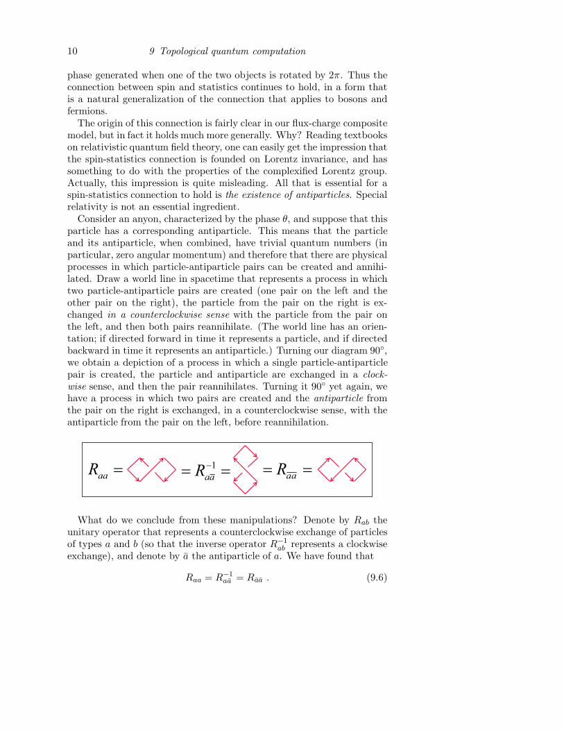
Consider an anyon, characterized by the phase θ, and suppose that thisparticle has a corresponding antiparticle. This means that the particleand its antiparticle, when combined, have trivial quantum numbers (inparticular, zero angular momentum) and therefore that there are physicalprocesses in which particle-antiparticle pairs can be created and annihi-lated. Draw a world line in spacetime that represents a process in whichtwo particle-antiparticle pairs are created (one pair on the left and theother pair on the right), the particle from the pair on the right is ex-changed in a counterclockwise sense with the particle from the pair onthe left, and then both pairs reannihilate. (The world line has an orien-tation; if directed forward in time it represents a particle, and if directedbackward in time it represents an antiparticle.) Turning our diagram 90◦,we obtain a depiction of a process in which a single particle-antiparticlepair is created, the particle and antiparticle are exchanged in a clock-
wise sense, and then the pair reannihilates. Turning it 90◦ yet again, wehave a process in which two pairs are created and the antiparticle fromthe pair on the right is exchanged, in a counterclockwise sense, with theantiparticle from the pair on the left, before reannihilation.
aaR1
aaR aaR
What do we conclude from these manipulations? Denote by Rab theunitary operator that represents a counterclockwise exchange of particlesof types a and b (so that the inverse operator R−1
ab represents a clockwiseexchange), and denote by a the antiparticle of a. We have found that
Raa = R−1aa = Raa . (9.6)
9.4 Combining anyons 11
If a is an anyon with exchange phase eiθ, then its antiparticle a also hasthe same exchange phase. Furthermore, when a and a are exchangedcounterclockwise, the phase acquired is e−iθ.
These conclusions are unsurprising when we interpret them from theperspective of our flux-charge composite model of anyons. The antipar-ticle of the object with flux Φ and charge q has flux −Φ and charge −q.Hence, when we exchange two antiparticles, the minus signs cancel andthe effect is the same as though the particles were exchanged. But if weexchange a particle and an antiparticle, then the relative sign of chargeand flux results in the exchange phase e−iqΦ = e−iθ.
But what is the connection between these observations about statisticsand the spin? Continuing to contemplate the same spacetime diagram, letus consider its implications regarding the orientation of the particles. Forkeeping track of the orientation, it is convenient to envision the particleworld line not as a thread but as a ribbon in spacetime. I claim that ourprocess can be smoothly deformed to one in which a particle-antiparticlepair is created, the particle is rotated counterclockwise by 2π, and thenthe pair reannihilates. A convenient way to verify this assertion is to takeoff your belt (or borrow a friend’s). The buckle at one end specifies anorientation; point your thumb toward the buckle, and following the right-hand rule, twist the belt by 2π before rebuckling it. You should be ableto check that you can lay out the belt to match the spacetime diagram forany of the exchange processes described earlier, and also for the processin which the particle rotates by 2π.
Thus, in a topological sense, rotating a particle counterclockwise by 2πis really the same thing as exchanging two particles in a counterclockwisesense (or exchanging particle and antiparticle in a clockwise sense), whichprovides a satisfying explanation for a general spin-statistics connection.†
I emphasize again that this argument invokes processes in which particle-antiparticle pairs are created and annihilated, and therefore the existenceof antiparticles is an essential prerequisite for it to apply.
9.4 Combining anyons
We know that a composite object composed of two fermions is a bo-son. What happens when we build a composite object by combining twoanyons?
† Actually, this discussion has been oversimplified. Though it is adequate for abeliananyons, we will see that it must be amended for nonabelian anyons, because Rab hasmore than one eigenvalue in the nonabelian case. Similarly, the discussion in the nextsection of “combining anyons” will need to be elaborated because, in the nonabeliancase, more than one kind of composite anyon can be obtained when two anyons arefused together.
12 9 Topological quantum computation
Suppose that a is an anyon with exchange phase eiθ, and that we builda “molecule” from n of these a anyons. What phase is acquired under acounterclockwise exchange of the two molecules?
The answer is clear in our flux-charge composite model. Each of the ncharges in one molecule acquires a phase eiθ/2 when transported half wayaround each of the n fluxes in the other molecule. Altogether then, 2n2
factors of the phase eiθ/2 are generated, resulting in the total phase
eiθn = ein2θ . (9.7)
Said another way, the phase eiθ occurs altogether n2 times because ineffect n anyons in one molecule are being exchanged with n anyons inthe other molecule. Contrary to what we might have naively expected, ifwe split a fermion (say) into two identical constituents, the constituentshave, not an exchange phase of
√−1 = i, but rather (eiπ)1/4 = eiπ/4.
This behavior is compatible with the spin-statistics connection: theangular momentum J of the n-anyon molecule satisfies
e−2πiJn = e−2πin2J = ein2θ . (9.8)
For example, consider a molecule of two anyons, and imagine rotatingthe molecule counterclockwise by 2π. Not only does each anyon in themolecule rotate by 2π; in addition one of the anyons revolves around theother. One revolution is equivalent to two successive exchanges, so thatthe phase generated by the revolution is ei2θ. The total effect of the tworotations and the revolution is the phase
exp [i (θ + θ + 2θ)] = ei4θ . (9.9)
Another way to understand why the angular momenta of the anyons inthe molecule do not combine additively is to note that the total angularmomentum of the molecule consists of two parts — the spin angularmomentum S of each of the two anyons (which is additive) and the orbital
angular momentum L of the anyon pair. Because the counterclockwisetransport of one anyon around the other generates the nontrivial phaseei2θ, the dependence of the two-anyon wavefunction ψ on the relativeazimuthal angle ϕ is not single-valued; instead,
ψ(ϕ+ 2π) = e−i2θψ(ϕ) . (9.10)
This means that the spectrum of the orbital angular momentum L isshifted away from integer values:
e−i2πL = e2iθ , (9.11)
9.5 Unitary representations of the braid group 13
and this orbital angular momentum combines additively with the spin Sto produce the total angular momentum
−2πJ = −2πL−2πS = 2θ+2θ+ 2π(integer) = 4θ+ 2π(integer) . (9.12)
What if, on the other hand, we build a molecule aa from an anyon aand its antiparticle a? Then, as we’ve seen, the spin S has the same valueas for the aa molecule. But the exchange phase has the opposite value, sothat the noninteger part of the orbital angular momentum is −2πL = −2θinstead of −2πL = 2θ, and the total angular momentum J = L + S isan integer. This property is necessary, of course, if the aa pair is to beable to annihilate without leaving behind an object that carries nontrivialangular momentum.
9.5 Unitary representations of the braid group
We have already noted that the angular momentum spectrum has differ-ent properties in two spatial dimensions than in three dimensions becauseSO(2) has different topological properties than SO(3) (SO(3) has a com-pact simply connected covering group SU(2), but SO(2) does not). Thisobservation provides one way to see why anyons are possible in two di-mensions but not in three. It is also instructive to observe that particleexchanges have different topological properties in two spatial dimensionsthan in three dimensions.
As we have found in our discussion of the relation between the statisticsof particles and of antiparticles, it is useful to envision exchanges of parti-cles as processes taking place in spacetime. In particular, it is convenientto imagine that we are computing the quantum transition amplitude fora time-dependent process involving n particles by evaluating a sum overparticle histories (though for our purposes it will not actually be necessaryto calculate any path integrals).
Consider a system of n indistinguishable pointlike particles confined toa two-dimensional spatial surface (which for now we may assume is theplane), and suppose that no two particles are permitted to occupy coinci-dent positions. We may think of a configuration of the particles at a fixedtime as a plane with n “punctures” at specified locations — that is, weassociate with each particle a hole in the surface with infinitesimal radius.The condition that the particles are forbidden to coincide is enforced bydemanding that there are exactly n punctures in the plane at any time.Furthermore, just as the particles are indistinguishable, each punctureis the same as any other. Thus if we were to perform a permutation ofthe n punctures, this would have no physical effect; all the punctures arethe same anyway, so it makes no difference which one is which. All thatmatters is the n distinct particle positions in the plane.
14 9 Topological quantum computation
To evaluate the quantum amplitude for a configuration of n particlesat specified initial positions at time t = 0 to evolve to a configurationof n particles at specified final positions at time t = T , we are to sumover all classical histories for the n particles that interpolate between thefixed initial configuration and the fixed final configuration, weighted bythe phase eiS, where S is the classical action of the history. If we envisioneach particle world line as a thread, each history for the n particles be-comes a braid, where each particle on the initial (t = 0) time slice can beconnected by a thread to any one of the particles on the final (t = T ) timeslice. Furthermore, since the particle world lines are forbidden to cross,the braids fall into distinct topological classes that cannot be smoothlydeformed one to another, and the path integral can be decomposed asa sum of contributions, with each contribution arising from a differenttopological class of histories.
Nontrivial exchange operations acting on the particles on the final timeslice change the topological class of the braid. Thus we see that theelements of the symmetry group generated by exchanges are in one-to-onecorrespondence with the topological classes. This (infinite) group is calledBn, the braid group on n strands; the group composition law correspondsto concatenation of braids (that is, following one braid with another). Inthe quantum theory, the quantum state of the n indistinguishable particlesbelongs to a Hilbert space that transforms as a unitary representation ofthe braid group Bn.
The group can be presented as a set of generators that obey particulardefining relations. To understand the defining relations, we may imag-ine that the n particles occupy n ordered positions (labeled 1, 2, 3, . . . , n)arranged on a line. Let σ1 denote a counterclockwise exchange of theparticles that initially occupy positions 1 and 2, let σ2 denote a counter-clockwise exchange of the particles that initially occupy positions 2 and3, and so on. Any braid can be constructed as a succession of exchangesof neighboring particles; hence σ1, σ2, . . . , σn−1 are the group generators.
The defining relations satisfied by these generators are of two types.The first type is
σjσk = σkσj , |j − k| ≥ 2 , (9.13)
which just says that exchanges of disjoint pairs of particles commute. Thesecond, slightly more subtle, type of relation is
σjσj+1σj = σj+1σjσj+1 , j = 1, 2, . . . , n− 2 , (9.14)
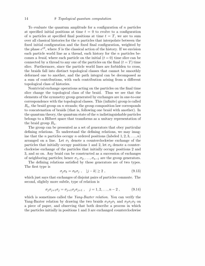
which is sometimes called the Yang-Baxter relation. You can verify theYang-Baxter relation by drawing the two braids σ1σ2σ1 and σ2σ1σ2 ona piece of paper, and observing that both describe a process in whichthe particles initially in positions 1 and 3 are exchanged counterclockwise
9.5 Unitary representations of the braid group 15
about the particle labeled 2, which stays fixed — i.e., these are topologi-cally equivalent braids.
2
1
2
1
2
1
Since the braid group is infinite, it has an infinite number of unitaryirreducible representations, and in fact there are an infinite number of one-
dimensional representations. Indistinguishable particles that transform asa one-dimensional representation of the braid group are said to be abelian
anyons. In the one-dimensional representations, each generator σj ofBn isrepresented by a phase σj = eiθj . Furthermore, the Yang-Baxter relationbecomes eiθjeiθj+1eiθj = eiθj+1eiθjeiθj+1 , which implies eiθj = eiθj+1 ≡ eiθ
— all exchanges are represented by the same phase. Of course, thatmakes sense; if the particles are really indistinguishable, the exchangephase ought not to depend on which pair is exchanged. For θ = 0 weobtain bosons, and for θ = π, fermions
The braid group also has many nonabelian representations that areof dimension greater than one; indistinguishable particles that transformas such representations are said to be nonabelian anyons (or, sometimes,nonabelions). To understand the physical properties of nonabelian anyonswe will need to understand the mathematical structure of some of theserepresentations. In these lectures, I hope to convey some intuition aboutnonabelian anyons by discussing some examples in detail.
For now, though, we can already anticipate the main goal we hope tofulfill. For nonabelian anyons, the irreducible representation of Bn real-ized by n anyons acts on a “topological vector space” Vn whose dimensionDn increases exponentially with n. And for anyons with suitable prop-erties, the image of the representation may be dense in SU(Dn). Thenbraiding of anyons can simulate a quantum computation — any (special)unitary transformation acting on the exponentially large vector space Vn
can be realized with arbitrarily good fidelity by executing a suitably cho-sen braid.
Thus we are keenly interested in the nonabelian representations of thebraid group. But we should also emphasize (and will discuss at greater
16 9 Topological quantum computation
length later on) that there is more to a model of anyons than a mere rep-resentation of the braid group. In our flux tube model of abelian anyons,we were able to describe not only the effects of an exchange of anyons, butalso the types of particles that can be obtained when two or more anyonsare combined together. Likewise, in a general anyon model, the anyonsare of various types, and the model incorporates “fusion rules” that spec-ify what types can be obtained when two anyons of particular types arecombined. Nontrivial consistency conditions arise because fusion is asso-ciate (fusing a with b and then fusing the result with c is equivalent tofusing b with c and then fusing the result with a), and because the fusionrules must be consistent with the braiding rules. Though these consis-tency conditions are highly restrictive, many solutions exist, and hencemany different models of nonabelian anyons are realizable in principle.
9.6 Topological degeneracy
But before moving on to nonabelian anyons, there is another importantidea concerning abelian anyons that we should discuss. In any model ofanyons (indeed, in any local quantum system with a mass gap), there is aground state or vacuum state, the state in which no particles are present.On the plane the ground state is unique, but for a two-dimensional surfacewith nontrivial topology, the ground state is degenerate, with the degree ofdegeneracy depending on the topology. We have already encountered thisphenomenon of “topological degeneracy” in the model of abelian anyonsthat arose in our study of a particular quantum error-correcting code,Kitaev’s toric code. Now we will observe that topological degeneracy is ageneral feature of any model of (abelian) anyons.
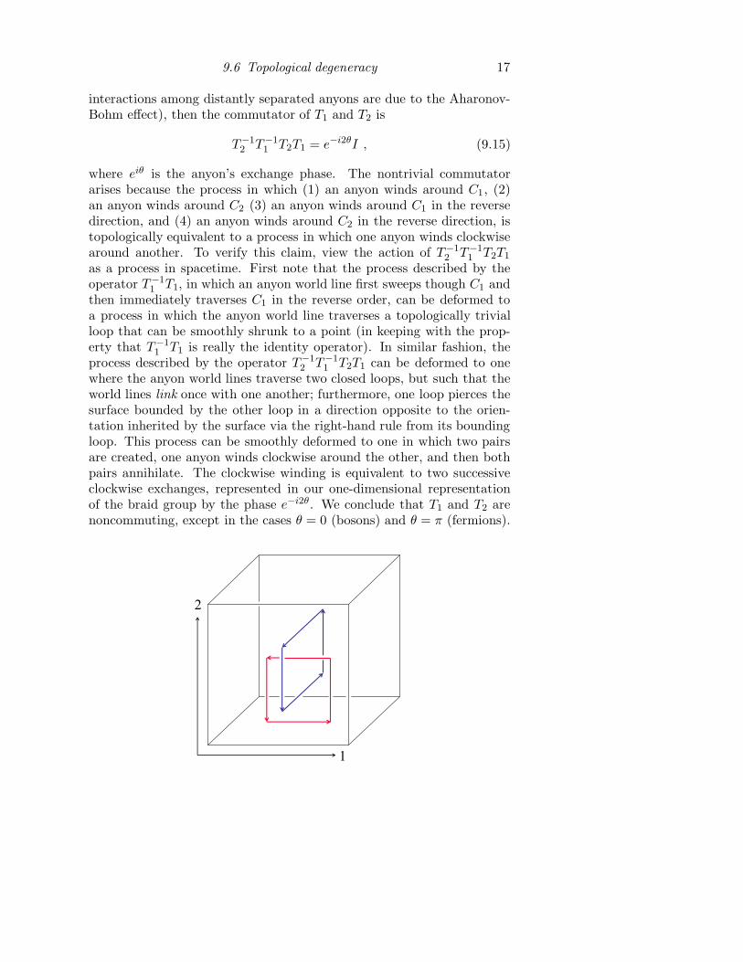
We can arrive at the concept of topological degeneracy by examiningthe representations of a simple operator algebra. Consider the case of thetorus, represented as a square with opposite sides identified, and considerthe two fundamental 1-cycles of the torus: C1, which winds around thesquare in the x1 direction, and C2 which winds around in the x2 direction.A unitary operator T1 can be constructed that describes a process inwhich an anyon-antianyon pair is created, the anyon propagates aroundC1, and then the pair reannihilates. Similarly a unitary operator T2 canbe constructed that describes a process in which the pair is created, andthe anyon propagates around the cycle C2 before the pair reannihilates.Each of the operators T1 and T2 preserves the ground state of the system(the state with no particles); indeed, each commutes with the HamiltonianH of the system and so either can be simultaneously diagonalized withH (T1 and T2 are both symmetries).
However, T1 and T2 do not commute with one another. If our torushas infinite spatial volume, and there is a mass gap (so that the only
9.6 Topological degeneracy 17
interactions among distantly separated anyons are due to the Aharonov-Bohm effect), then the commutator of T1 and T2 is
T−12 T−1
1 T2T1 = e−i2θI , (9.15)
where eiθ is the anyon’s exchange phase. The nontrivial commutatorarises because the process in which (1) an anyon winds around C1, (2)an anyon winds around C2 (3) an anyon winds around C1 in the reversedirection, and (4) an anyon winds around C2 in the reverse direction, istopologically equivalent to a process in which one anyon winds clockwisearound another. To verify this claim, view the action of T−1
2 T−11 T2T1
as a process in spacetime. First note that the process described by theoperator T−1
1 T1, in which an anyon world line first sweeps though C1 andthen immediately traverses C1 in the reverse order, can be deformed toa process in which the anyon world line traverses a topologically trivialloop that can be smoothly shrunk to a point (in keeping with the prop-erty that T−1
1 T1 is really the identity operator). In similar fashion, theprocess described by the operator T−1
2 T−11 T2T1 can be deformed to one
where the anyon world lines traverse two closed loops, but such that theworld lines link once with one another; furthermore, one loop pierces thesurface bounded by the other loop in a direction opposite to the orien-tation inherited by the surface via the right-hand rule from its boundingloop. This process can be smoothly deformed to one in which two pairsare created, one anyon winds clockwise around the other, and then bothpairs annihilate. The clockwise winding is equivalent to two successiveclockwise exchanges, represented in our one-dimensional representationof the braid group by the phase e−i2θ. We conclude that T1 and T2 arenoncommuting, except in the cases θ = 0 (bosons) and θ = π (fermions).
2
1
18 9 Topological quantum computation
Since T1 and T2 both commute with the Hamiltonian H , both preservethe eigenspaces of H , but since T1 and T2 do not commute with oneanother, they cannot be simultaneously diagonalized. Since T1 is unitary,its eigenvalues are phases; let us use the angular variable α ∈ [0, 2π) tolabel an eigenstate of T1 with eigenvalue eiα:
T1|α〉 = eiα|α〉 . (9.16)
Then applying T2 to the T1 eigenstate advances the value of α by 2θ:
T1 (T2|α〉) = ei2θT2T1|α〉 = ei2θeiα (T2|α〉) . (9.17)
Suppose that θ is a rational multiple of 2π, which we may express as
θ = πp/q , (9.18)
where q and p (p < 2q) are positive integers with no common factor. Thenwe conclude that T1 must have at least q distinct eigenvalues; T1 actingon α generates an orbit with q distinct values:
α+
(
2πp
q
)
k (mod 2π) , k = 0, 1, 2, . . . , q − 1 . (9.19)
Since T1 commutes with H , on the torus the ground state of our anyonicsystem (indeed, any energy eigenstate) must have a degeneracy that is aninteger multiple of q. Indeed, generically (barring further symmetries oraccidental degeneracies), the degeneracy is expected to be exactly q.
For a two-dimensional surface with genus g (a sphere with g “handles”),the degree of this topological degeneracy becomes qg, because there areoperators analogous to T1 and T2 associated with each of the g handles,and all of the T1-like operators can be simultaneously diagonalized. Fur-thermore, we can apply a similar argument to a finite planar medium ifsingle anyons can be created and destroyed at the edges of the system. Forexample, consider an annulus in which anyons can appear or disappearat the inner and outer edges. Then we could define the unitary opera-tor T1 as describing a process in which an anyon winds counterclockwisearound the annulus, and a unitary operator T2 as describing a process inwhich an anyon appears at the outer edge, propagates to the inner edge,and disappears. These operators T1 and T2 have the same commutatoras the corresponding operators defined on the torus, and so we concludeas before that the ground state on the annulus is q-fold degenerate forθ = πp/q. For a disc with h holes, there is an operator analogous toT1 that winds an anyon counterclockwise around each of the holes, andan operator analogous to T2 that propagates an anyon from the outerboundary of the disk to the edge of the hole; thus the degeneracy is qh.
9.6 Topological degeneracy 19
What we have described here is a robust topological quantum memory.The phase ei2θ = ei2πp/q ≡ ω acquired when one anyon winds counter-clockwise around another is a primitive qth root of unity, and in the caseof a planar system with holes, the operator T1 can be regarded as the en-coded Pauli operator Z acting on a q-dimension system associated witha particular hole. Physically, the eigenvalue ωs of Z just counts the num-ber s of anyons that are “stuck” inside the hole. The operator T2 canbe regarded as the complementary Pauli operator X that increments thevalue of s by carrying one anyon from the boundary of the system anddepositing it in the hole. Since the quantum information is encoded in anonlocal property of the system, it is well protected from environmentaldecoherence. By the same token depositing a quantum state in the mem-ory, and reading it out, might be challenging for this system, though inprinciple Z could be measured by, say, performing an interference experi-ment in which an anyon projectile scatters off of a hole. We will see laterthat by using nonabelian anyons we will be able to simplify the readout;in addition, with nonabelian anyons we can use topological properties toprocess quantum information as well as to store it.
Just how robust is this quantum memory? We need to worry about er-rors due to thermal fluctuations and due to quantum fluctuations. Ther-mal fluctuations might excite the creation of anyons, and thermal anyonsmight diffuse around one of the holes in the sample, or from one bound-ary to another, causing an encoded error. Thermal errors are heavilysuppressed by the Boltzman factor e−∆/T , if the temperature T is suffi-ciently small compared to the energy gap ∆ (the minimal energy cost ofcreating a single anyon at the edge of the sample, or a pair of anyons inthe bulk). The harmful quantum fluctuations are tunneling processes inwhich a virtual anyon-antianyon pair appears and the anyon propagatesaround a hole before reannihilating, or a virtual anyon appears at theedge of a hole and propagates to another boundary before disappearing.These errors due to quantum tunneling are heavily suppressed if the holesare sufficiently large and sufficiently well separated from one another andfrom the outer boundary.‡
Note that our conclusion that the topological degeneracy is finite hingedon the assumption that the angle θ is a rational multiple of π. We maysay that a theory of anyons is rational if the topological degeneracy isfinite for any surface of finite genus (and, for nonabelian anyons, if the
‡ If you are familiar with Euclidean path integral methods, you’ll find it easy to verifythat in the leading semiclassical approximation the amplitude A for such a tunnelingprocess in which the anyon propagates a distance L has the form A = Ce
−L/L0 ,where C is a constant and L0 = h (2m
∗∆)−1/2; here h is Planck’s constant and m∗
is the effective mass of the anyon, defined so that the kinetic energy of an anyontraveling at speed v is 1
2m
∗v2.
20 9 Topological quantum computation
topological vector space Vn is finite-dimensional for any finite number ofanyons n). We may anticipate that the anyons that arise in any physicallyreasonable system will be rational in this sense, and therefore should beexpected to have exchange phases that are roots of unity.
9.7 Toric code revisited
If these observations about topological degeneracy seem hauntingly famil-iar, it may be because we used quite similar arguments in our discussionof the toric code.
The toric code can be regarded as the (degenerate) ground state of asystem of qubits that occupy the links of a square lattice on the torus,with Hamiltonian
H = −1
4∆
(
∑
P
ZP +∑
S
XS
)
, (9.20)
where the plaquette operator ZP = ⊗`∈PZ` is the tensor product of Z’sacting on the four qubits associated with the links contained in plaquetteP , and the site operator XS ⊗`3S X` is the tensor product of X ’s actingon the four qubits associated with the links that meet at the site S. Theseplaquette and site operators are just the (commuting) stabilizer generatorsfor the toric code. The ground state is the simultaneous eigenstate witheigenvalue 1 of all the stabilizer generators.
This model has two types of localized particle excitations — plaquetteexcitations where ZP = −1, which we might think of as magnetic fluxons,and site excitations where XS = −1, which we might think of as electriccharges. A Z error acting on a link creates a pair of charges on the twosite joined by the link, and an X error acting on a link creates a pair offluxons on the two plaquettes that share the link. The energy gap ∆ isthe cost of creating a pair of either type.
The charges are bosons relative to one another (they have a trivialexchange phase eiθ = 1), and the fluxons are also bosons relative to oneanother. Since the fluxons are distinguishable from the charges, it doesnot make sense to exchange a charge with a flux. But what makes thisan anyon model is that a phase (−1) is acquired when a charge is carriedaround a flux. The degeneracy of the ground state (the dimension of thecode space) can be understood as a consequence of this property of theparticles.
For this model on the torus, because there are two types of particles,there are two types of T1 operators: T1,S, which propagates a charge (sitedefect) around the 1-cycle C1, and T1,P , which propagates a fluxon (pla-quette defect) around C1. Similarly there are two types of T2 operators,
9.8 The nonabelian Aharonov-Bohm effect 21
T2,S and T2,P . The nontrivial commutators are
T−12,PT
−11,ST2,PT1,S = −1 = T−1
2,ST−11,PT2,ST1,P , (9.21)
both arising from processes in which world lines of charges and fluxon linkonce with one another. Thus T1,S and T2,S can be diagonalized simulta-neously, and can be regarded as the encoded Pauli operators Z1 and Z2
acting on two protected qubits. The operator T2,P , which commutes withZ1 and anticommutes with Z2, can be regarded as the encoded X1, andsimilarly T1,P is the encoded X2.
On the torus, the degeneracy of the four ground states is exact forthe ideal Hamiltonian we constructed (the particles have infinite effectivemasses). Weak local perturbations will break the degeneracy, but onlyby an amount that gets exponentially small as the linear size L of thetorus increases. To be concrete, suppose the perturbation is a uniform“magnetic field” pointing in the z direction, coupling to the magneticmoments of the qubits:
H ′ = −h∑
`
Z` . (9.22)
Because of the nonzero energy gap, for the purpose of computing in per-turbation theory the leading contribution to the splitting of the degen-eracy, it suffices to consider the effect of the perturbation in the four-dimensional subspace spanned by the ground states of the unperturbedsystem. In the toric code, the operators with nontrivial matrix elementsin this subspace are those such that Z`’s act on links that form a closedloop that wraps around the torus (or X`’s act on links whose dual linksform a closed loop that wraps around the torus). For an L×L lattice onthe torus, the minimal length of such a closed loop is L; therefore nonva-nishing matrix elements do not arise in perturbation theory until the Lthorder, and are suppressed by hL. Thus, for small h and large L, memoryerrors due to quantum fluctuations occur only with exponentially smallamplitude.
9.8 The nonabelian Aharonov-Bohm effect
There is a beautiful abstract theory of nonabelian anyons, and in duecourse we will delve into that theory a bit. But I would prefer to launchour study of the subject by describing a more concrete model.
With that goal in mind, let us recall some properties of chromodynam-
ics, the theory of the quarks and gluons contained within atomic nucleiand other strongly interacting particles. In the real world, quarks are per-manently bound together and can never be isolated, but for our discussionlet us imagine a fictitious world in which the forces between quarks are
22 9 Topological quantum computation
weak, so that the characteristic distance scale of quark confinement isvery large.
Quarks carry a degree of freedom known metaphorically as color. Thatis, there are three kinds of quarks, which in keeping with the metaphorwe call red (R), yellow (Y ), and blue (B). Quarks of all three colors arephysical identical, except that when we bring two quarks together, we cantell whether their colors are the same (the Coulombic interaction betweenlike colors is repulsive), or different (distinct colors attract). There isnothing to prevent me from establishing a quark bureau of standards inmy laboratory, where colored quarks are sorted into three bins; all thequarks in the same bin have the same color, and quarks in different binshave different colors. We may attach (arbitrary) labels to the three bins— R, Y , and B.
If while taking a hike outside by lab, I discover a previously unseenquark, I may at first be unsure of its color. But I can find out. I capturethe quark and carry it back to my lab, being very careful not to disturbits color along the way (in chromodynamics, there is a notion of parallel
transport of color). Once back at the quark bureau of standards, I cancompare this new quark to the previously calibrated quarks in the bins,and so determine whether the new quark should be labeled R, Y , or B.
It sounds simple but there is a catch: in chromodynamics, the paral-lel transport of color is path dependent due to an Aharonov-Bohm phe-nomenon that affects color. Suppose that at the quark bureau of stan-dards a quark is prepared whose color is described by the quantum state
|ψq〉 = qR|R〉+ qY |Y 〉+ qB |B〉 ; (9.23)
it is a coherent superposition with amplitudes qR, qY , qB for the red, yel-low, and blue states. The quark is carried along a path that winds arounda color magnetic flux tube and is returned to the quark bureau of stan-dards where its color can be recalibrated. Upon its return the color statehas been rotated:
q′Rq′Yq′B
= U
qRqYqB
, (9.24)
where U is a (special) unitary 3 × 3 matrix. Similarly, when a newlydiscovered quark is carried back to the bureau of standards, the outcomeof a measurement of its color will depend on whether it passed to the leftor the right of the flux tube during its voyage.
This path dependence of the parallel transport of color is closely analo-gous to the path dependence of the parallel transport of a tangent vectoron a curved Riemannian manifold. In chromodynamics, a magnetic fieldis the “curvature” whose strength determines the amount of path depen-dence.
9.8 The nonabelian Aharonov-Bohm effect 23
In general, the SU(3) matrix U that describes the effect of paralleltransport of color about a closed path depends on the basepoint x0 wherethe path begins and ends, as well as on the closed loop C traversed by thepath — when it is important to specify the loop and basepoint we will usethe notation U(C, x0). The eigenvalues of the matrix U have an invariant“geometrical” meaning characterizing the parallel transport, but U itselfdepends on the conventions we have established at the basepoint. Youmight prefer to choose a different orthonormal basis for the color spaceat the basepoint x0 than the basis I chose, so that your standard colorsR, Y , and B differ from mine by the action of an SU(3) matrix V (x0).Then, while I characterize the effect or parallel transport around the loopC with the matrix U , you characterize it with another matrix
V (x0)U(C, x0)V (x0)−1 , (9.25)
that differs from mine by conjugation by V (x0). Physicists sometimesspeak of this freedom to redefine conventions as a choice of gauge, and saythat U itself is gauge dependent while its eigenvalues are gauge invariant.
Chromodynamics, on the distance scales we consider here (much smallerthan the characteristic distance scale of quark confinement), is a the-ory like electrodynamics with long-range Coulombic interactions amongquarks, mediated by “gluon” fields. We will prefer to consider a theorythat retains some of the features of chromodynamics (in particular thepath dependence of color transport), but without the easily excited lightgluons. In the case of electrodynamics, we eliminated the light photonby considering a “superconductor” in which charged particles form a con-densate, magnetic fields are expelled, and the magnetic flux of an isolatedobject is quantized. Let us appeal to the same idea here. We consider anonabelian superconductor in two spatial dimensions. This world containsparticles that carry “magnetic flux” (similar to the color magnetic flux inchromodynamics) and particles that carry charge (similar to the coloredquarks of chromodynamics). The flux takes values in a nonabelian finite
group G, and the charges are unitary irreducible representations of thegroup G. In this setting, we can formulate some interesting models ofnonabelian anyons.
Let R denote a particular irreducible representation of G, whose di-mension is denoted |R|. We may establish a “charge bureau of stan-dards,” and define there an arbitrarily chosen orthonormal basis for the|R|-dimensional vector space acted upon by R:
|R, i〉 , i = 1, 2, . . . |R| . (9.26)
When a charge R is transported around a closed path that encloses a fluxa ∈ G, there is a nontrivial Aharonov-Bohm effect — the basis for R is
24 9 Topological quantum computation
rotated by a unitary matrix DR(a) that represents a:
|R, j〉 7→|R|∑
i=1
|R, i〉DRij(a) . (9.27)
The matrix elements DRij(a) are measurable in principle, for example by
conducting interference experiments in which a beam of calibrated chargescan pass on either side of the flux. (The phase of the complex numberDR
ij(a) determines the magnitude of the shift of the interference fringes,
and the modulus of DRij(a) determines the visibility of the fringes.) Thus
once we have chosen a standard basis for the charges, we can use thecharges to attach labels (elements of G) to all fluxes. The flux labelsare unambiguous as long as the representation R is faithful, and barringany group automorphisms (which create ambiguities that we are free toresolve however we please).
However, the group elements that we attach to the fluxes depend on ourconventions. Suppose I am presented with k fluxons (particles that carryflux), and that I use my standard charges to measure the flux of eachparticle. I assign group elements a1, a2, . . . , ak ∈ G to the k fluxons. Youare then asked to measure the flux, to verify my assignments. But yourstandard charges differ from mine, because they have been surreptitiouslytransported around another flux (one that I would label with g ∈ G).Therefore you will assign the group elements ga1g
−1, ga2g−1, . . . , gakg
−1
to the k fluxons; our assignments differ by an overall conjugation by g.The moral of this story is that the assignment of group elements to
fluxons is inherently ambiguous and has no invariant meaning. But be-cause the valid assignments of group elements to fluxons differ only byconjugation by some element g ∈ G, the conjugacy class of the flux inG does have an invariant meaning on which all observers will agree. In-deed, even if we fix our conventions at the charge bureau of standards, thegroup element that we assign to a particular fluxon may change if thatfluxon takes part in a physical process in which it braids with other flux-ons. For that reason, the fluxons belonging to the same conjugacy classshould all be regarded as indistinguishable particles, even though theycome in many varieties (one for each representative of the class) that canbe distinguished when we make measurements at a particular time andplace: The fluxons are nonabelian anyons.
9.9 Braiding of nonabelian fluxons
We will see that, for a nonabelian superconductor with suitable properties,it is possible to operate a fault-tolerant universal quantum computer by
9.9 Braiding of nonabelian fluxons 25
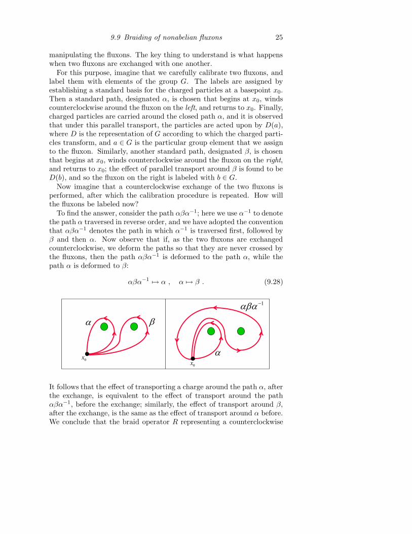
manipulating the fluxons. The key thing to understand is what happenswhen two fluxons are exchanged with one another.
For this purpose, imagine that we carefully calibrate two fluxons, andlabel them with elements of the group G. The labels are assigned byestablishing a standard basis for the charged particles at a basepoint x0.Then a standard path, designated α, is chosen that begins at x0, windscounterclockwise around the fluxon on the left, and returns to x0. Finally,charged particles are carried around the closed path α, and it is observedthat under this parallel transport, the particles are acted upon by D(a),where D is the representation of G according to which the charged parti-cles transform, and a ∈ G is the particular group element that we assignto the fluxon. Similarly, another standard path, designated β, is chosenthat begins at x0, winds counterclockwise around the fluxon on the right,and returns to x0; the effect of parallel transport around β is found to beD(b), and so the fluxon on the right is labeled with b ∈ G.
Now imagine that a counterclockwise exchange of the two fluxons isperformed, after which the calibration procedure is repeated. How willthe fluxons be labeled now?
To find the answer, consider the path αβα−1; here we use α−1 to denotethe path α traversed in reverse order, and we have adopted the conventionthat αβα−1 denotes the path in which α−1 is traversed first, followed byβ and then α. Now observe that if, as the two fluxons are exchangedcounterclockwise, we deform the paths so that they are never crossed bythe fluxons, then the path αβα−1 is deformed to the path α, while thepath α is deformed to β:
αβα−1 7→ α , α 7→ β . (9.28)
0x
0x
1
It follows that the effect of transporting a charge around the path α, afterthe exchange, is equivalent to the effect of transport around the pathαβα−1, before the exchange; similarly, the effect of transport around β,after the exchange, is the same as the effect of transport around α before.We conclude that the braid operator R representing a counterclockwise
26 9 Topological quantum computation
exchange acts on the fluxes according to
R : |a, b〉 → |aba−1, a〉 . (9.29)
Of course, if the fluxes a and b are commuting elements of G, all thebraiding does is swap the positions of the two labels. But if a and b do notcommute, the effect of the exchange is more subtle and interesting. Theasymmetric form of the action of R is a consequence of our conventionsand of the (counterclockwise) sense of the exchange; the inverse operatorR−1 representing a clockwise exchange acts as
R−1 : |a, b〉 → |b, b−1ab〉 . (9.30)
Note that the total flux of the pair of fluxons can be detected by a chargedparticle that traverses the path αβ that encloses both members of thepair. Since in principle the charge detecting this total flux could be far,far away, the exchange ought not to alter the total flux; indeed, we findthat the product flux ab is preserved by R and by R−1.
The effect of two successive counterclockwise exchanges is the “mon-odromy” operator R2, representing the counterclockwise winding of onefluxon about the other, whose action is
R2 : |a, b〉 7→ |(ab)a(ab)−1, (ab)b(ab)−1〉 ; (9.31)
both fluxes are conjugated by the total flux ab. That is, winding a coun-terclockwise about b conjugates b by a (and similarly, winding b clockwiseabout a conjugates a by b−1). The nontrivial monodromy means that ifmany fluxons are distributed in the plane, and one of these fluxons is tobe brought to my laboratory for analysis, the group element I assign tothe fluxon may depend on the path the flux follows as it travels to my lab.If for one choice of path the flux is labeled by a ∈ G, then for other pathsany other element bab−1 might in principle be assigned. Thus, the conju-gacy class in G represented by the fluxon is invariant, but the particularrepresentative of that class is ambiguous.
For example, suppose the group is G = S3, the permutation groupon three objects. One of the conjugacy classes contains all of the two-cycle permutations (transpositions of two objects), the three elements{(12), (23), (31)}. When two such two-cycles fluxes are combined, thereare three possibilities for the total flux — the trivial flux e, or one of thethree-cycle fluxes (123) or (132). If the total flux is trivial, the braidingof the two fluxes is also trivial (a and b = a−1 commute). But if the totalflux is nontrivial, then the braid operator R has orbits of length three:
R : |(12), (23)〉 7→ |(31), (12)〉 7→ |(23), (31)〉 7→ |(12), (23)〉 ,R : |(23), (12)〉 7→ |(31), (23)〉 7→ |(12), (31)〉 7→ |(23), (12)〉 ,
(9.32)
9.9 Braiding of nonabelian fluxons 27
Thus, if the two fluxons are exchanged three times, they swap positions(the number of exchanges is odd), yet the labeling of the state is unmod-ified. This observation means that there can be quantum interferencebetween the “direct” and “exchange” scattering of two fluxons that carrydistinct labels in the same conjugacy class, reinforcing the notion thatfluxes carrying conjugate labels ought to be regarded as indistinguishableparticles.
Since the braid operator acting on pairs of two-cycle fluxes satisfiesR3 = I , its eigenvalues are third roots of unity. For example, by takinglinear combinations of the three states with total flux (123), we obtainthe R eigenstates
R = 1 : |(12), (23)〉 + |(31), (12)〉 + |(23), (31)〉 ,R = ω : |(12), (23)〉+ ω|(31), (12)〉+ ω|(23), (31)〉 ,R = ω : |(12), (23)〉+ ω|(31), (12)〉+ ω|(23), (31)〉 , (9.33)
where ω = e2πi/3.Although a pair of fluxes |a, a−1〉 with trivial total flux has trivial braid-
ing properties, it is interesting for another reason — it carries charge. Theway to detect the charge of an object is to carry a flux b around the ob-ject (counterclockwise); this modifies the object by the action ofDR(b) forsome representation R of G. If the charge is zero then the representationis trivial — D(b) = I for all b ∈ G. But if we carry flux b counterclockwisearound the state |a, a−1〉, the state transforms as
|a, a−1〉 7→ |bab−1, ba−1b−1〉 , (9.34)
a nontrivial action (for at least some b) if a belongs to a conjugacy classwith more than one element. In fact, for each conjugacy class α, there isa unique state |0;α〉 with zero charge, the uniform superposition of theclass representatives:
|0;α〉 =1
√
|α|∑
a∈α
|a, a−1〉 , (9.35)
where |α| denotes the order of α. A pair of fluxons in the class α that canbe created in a local process must not carry any conserved charges andtherefore must be in the state |0;α〉. Other linear combinations orthogonalto |0;α〉 carry nonzero charge. This charge carried by a pair of fluxons canbe detected by other fluxons, yet oddly the charge cannot be localized onthe core of either particle in the pair. Rather it is a collective property ofthe pair. If two fluxons with a nonzero total charge are brought together,complete annihilation of the pair will be forbidden by charge conservation,even though the total flux is zero.
28 9 Topological quantum computation
In the case of a pair of fluxons from the two-cycle class of G = S3, forexample, there is a two-dimensional subspace with trivial total flux andnontrivial charge, for which we may choose the basis
|0〉 = |(12), (12)〉+ ω|(23), (23)〉+ ω|(31), (31)〉 ,|1〉 = |(12), (12)〉+ ω|(23), (23)〉+ ω|(31), (31)〉 . (9.36)
If a flux b is carried around the pair, both fluxes are conjugated by b;therefore the action (by conjugation) of S3 on these states is
D(12) =
(
0 11 0
)
, D(23) =
(
0 ωω 0
)
, D(31) =
(
0 ωω 0
)
,
D(123) =
(
ω 00 ω
)
, D(132) =
(
ω 00 ω
)
. (9.37)
This action is just the two-dimensional irreducible representation R = [2]of S3, and so we conclude that the charge of the pair of fluxons is [2].
Furthermore, under braiding this charge carried by a pair of fluxons canbe transferred to other particles. For example, consider a pair of particles,each of which carries charge but no flux (I will refer to such particles aschargeons), such that the total charge of the pair is trivial. If one ofthe chargeons transforms as the unitary irreducible representation R ofG, there is a unique conjugate representation R that can be combinedwith R to give the trivial representation; if {|R, i〉} is a basis for R, thena basis {|R, i〉} can be chosen for R, such that the chargeon pair withtrivial charge can be expressed as
|0;R〉 =1
√
|R|∑
i
|R, i〉 ⊗ |R, i〉 . (9.38)
Imagine that we create a pair of fluxons in the state |0;α〉 and alsocreate a pair of chargeons in the state |0;R〉. Then we wind the chargeonwith charge R counterclockwise around the fluxon with flux in class α,and bring the two chargeons together again to see if they will annihilate.What happens?
For a fixed value a ∈ α of the flux, the effect of the winding on thestate of the two chargeons is
|0;R〉 7→ 1√
|R|∑
i,j
|R, j〉 ⊗ |R, i〉DRji(a) ; (9.39)
if the charge of the pair were now measured, the probability that zerototal charge would be found is the square of the overlap of this state with|0;R〉, which is
Prob(0) =
∣
∣
∣
∣
χR(a)
|R|
∣
∣
∣
∣
2
, (9.40)
9.10 Superselection sectors of a nonabelian superconductor 29
whereχR(a) =
∑
i
DRii (a) = tr DR(a) (9.41)
is the character of the representation R, evaluated at a. In fact, thecharacter (a trace) is unchanged by conjugation — it takes the same valuefor all a ∈ α. Therefore, eq. (9.40) is also the probability that the pair ofchargeons has zero total charge when one chargeon (initially a memberof a pair in the state |0;R〉) winds around one fluxon (initially a memberof a pair in the state |0;α〉). Of course, since the total charge of all fourparticles is zero and charge is conserved, after the winding the two pairshave opposite charges — if the pair of chargeons has total charge R′, thenthe pair of fluxons must have total charge R′, combined with R′ to givetrivial total charge. A pair of particles with zero total charge and flux canannihilate, leaving no stable particle behind, while a pair with nonzerocharge will be unable to annihilate completely. We conclude, then, thatif the world lines of a fluxon pair and a chargeon pair link once, theprobability that both pairs will be able to annihilate is given by eq. (9.40).This probability is less than one, provided that the representation of Ris not one dimensional and the class α is not represented trivially. Thusthe linking of the world lines induces an exchange of charge between thetwo pairs.
For example, in the case where α is the two-cycle class of G = S3 andR = [2] (the two-dimensional irreducible representation of S3), we seefrom eq. (9.37) that χ[2](α) = 0. Therefore, charge is transfered withcertainty; after the winding, both the fluxon pair and the chargeon pairtransform as R′ = [2].
9.10 Superselection sectors of a nonabelian superconductor
In our discussion so far of the nonabelian superconductor, we have beenconsidering two kinds of particles: fluxons, which carry flux but no charge,and chargeons, which carry charge but no flux. These are not the mostgeneral possible particles. It will be instructive to consider what happenswhen we build a composite particle by combining a fluxon with a chargeon.In particular, what is the charge of the composite? This question issurprisingly subtle; to answer cogently, we should think carefully abouthow the charge can be measured.
In principle, charge can be measured in an Aharonov-Bohm interferenceexperiment. We could hide the object whose charge is to be found behinda screen in between two slits, shoot a beam of carefully calibrated fluxonsat the screen, and detect the fluxons on the other side. From the shift andvisibility of the interference pattern revealed by the detected positions ofthe fluxons, we can determine DR(b) for each b ∈ G, and so deduce R.
30 9 Topological quantum computation
However, there is a catch if the object being analyzed carries a nontrivialflux a ∈ G as well as charge. Since carrying a flux b around the flux achanges a to bab−1, the two possible paths followed by the b flux do not
interfere, if a and b do not commute. After the b flux is detected, we couldcheck whether the a flux has been modified, and determine whether the bflux passed through the slit on the left or the slit on the right. Since theflux (a or bab−1) is correlated with the “which way” information (left orright slit), the interference is destroyed.
Therefore, the experiment reveals information about the charge only ifa and b commute. Hence the charge attached to a flux a is not describedas an irreducible representation of G; instead it is an irreducible repre-sentation of a subgroup of G, the normalizer N (a) of a in G, which isdefined as
N (a) = {b ∈ G|ab = ba} . (9.42)
The normalizers N (a) and N (bab−1) are isomorphic, so we may associatethe normalizer with a conjugacy class α of G rather than with a par-ticular element, and denote it as N (α). Therefore, each type of particlethat can occur in our nonabelian superconductor really has two labels:a conjugacy class α describing the flux, and an irreducible representa-tion R(α) of N (α) describing the charge. We say that α and R(α) labelthe superselection sectors of the theory, as these are the properties of alocalized object that must be conserved in all local physical processes.For particles that carry the labels (α, R(α)), it is possible to establish a“bureau of standards” where altogether |α| · |R(α)| ≡ d(α,R(α)) differentparticle species can be distinguished at a particular time and place —this number is called the dimension of the sector. But if these particlesare braided with other particles the species may change, while the labels(α, R(α)) remain invariant.
In any theory of anyons, a dimension can be assigned to each particletype, although as we will see, in general the dimension need not be aninteger, and may have no direct interpretation in terms the counting ofdistinct species of the same type. The total dimension D can be definedby summing over all types; in the case of a nonabelian superconductor wehave
D2 =∑
α
∑
R(α)
d2(α,R(α))
=∑
α
|α|2∑
R(α)
|R(α)|2 . (9.43)
Since the sum over the dimension squared for all irreducible representa-tions of a finite group is the order of the group, and the order of thenormalizer N (α) is |G|/|α|, we obtain
D2 =∑
α
|α| · |G| = |G|2 ; (9.44)
9.10 Superselection sectors of a nonabelian superconductor 31
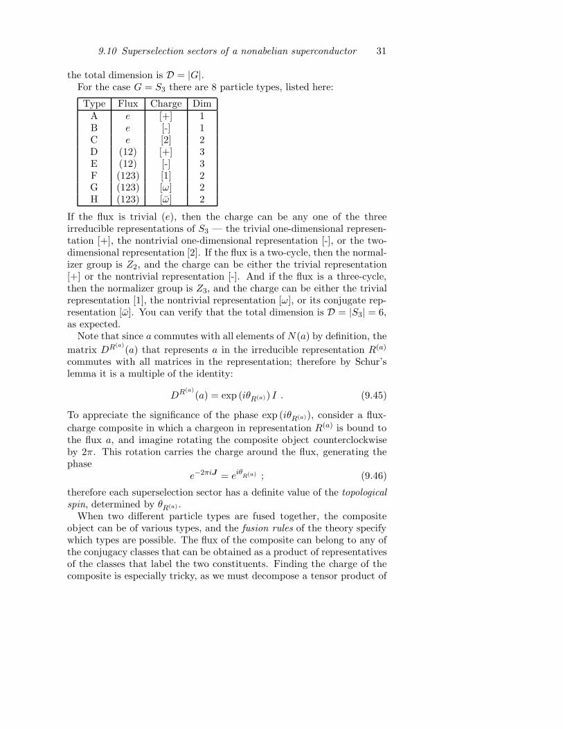
the total dimension is D = |G|.For the case G = S3 there are 8 particle types, listed here:
Type Flux Charge DimA e [+] 1B e [-] 1C e [2] 2D (12) [+] 3E (12) [-] 3F (123) [1] 2G (123) [ω] 2H (123) [ω] 2
If the flux is trivial (e), then the charge can be any one of the threeirreducible representations of S3 — the trivial one-dimensional represen-tation [+], the nontrivial one-dimensional representation [-], or the two-dimensional representation [2]. If the flux is a two-cycle, then the normal-izer group is Z2, and the charge can be either the trivial representation[+] or the nontrivial representation [-]. And if the flux is a three-cycle,then the normalizer group is Z3, and the charge can be either the trivialrepresentation [1], the nontrivial representation [ω], or its conjugate rep-resentation [ω]. You can verify that the total dimension is D = |S3| = 6,as expected.
Note that since a commutes with all elements of N (a) by definition, the
matrix DR(a)(a) that represents a in the irreducible representation R(a)
commutes with all matrices in the representation; therefore by Schur’slemma it is a multiple of the identity:
DR(a)(a) = exp (iθR(a)) I . (9.45)
To appreciate the significance of the phase exp (iθR(a)), consider a flux-
charge composite in which a chargeon in representation R(a) is bound tothe flux a, and imagine rotating the composite object counterclockwiseby 2π. This rotation carries the charge around the flux, generating thephase
e−2πiJ = eiθR(a) ; (9.46)
therefore each superselection sector has a definite value of the topological
spin, determined by θR(a) .When two different particle types are fused together, the composite
object can be of various types, and the fusion rules of the theory specifywhich types are possible. The flux of the composite can belong to any ofthe conjugacy classes that can be obtained as a product of representativesof the classes that label the two constituents. Finding the charge of thecomposite is especially tricky, as we must decompose a tensor product of
32 9 Topological quantum computation
representations of two different normalizer groups as a sum of representa-tions of the normalizer of the product flux. In the case G = S3, the rulegoverning the fusion of two particles of type D, for example, is
D ×D = A+ C + F +G+H (9.47)
We have already noted that the fusion of two two-cycle fluxes can yieldeither a trivial total flux or a three-cycle flux, and that the charge of thecomposite with trivial total flux can be either [+] or [2]. If the total fluxis a three-cycle, then the charge eigenstates are just the braid operatoreigenstates that we constructed in eq. (9.33).
For a system of two anyons, why should the eigenstates of the totalcharge also be eigenstates of the braid operator? We can understand thisconnection more generally by thinking about the angular momentum ofthe two-anyon composite object. The monodromy operator R2 capturesthe effect of winding one particle counterclockwise around another. Thiswinding is almost the same thing as rotating the composite system coun-terclockwise by 2π, except that the rotation of the composite system alsorotates both of the constituents. We can compensate for the rotation ofthe constituents by following the counterclockwise rotation of the compos-ite by a clockwise rotation of the constituents. Therefore, the monodromyoperator can be expressed as
(Rcab)
2 = e−2πiJce2πiJae2πiJb = ei(θc−θa−θb) . (9.48)
Here Rcab denotes the braid operator for a counterclockwise exchange of
particles of types a and b that are combined together into a compositeof type c, and we are using a more succinct notation than before, inwhich a, b, c are complete labels for the superselection sectors (specifying,in the nonabelian superconductor model, both the flux and the charge).Since each superselection sector has a definite topological spin, and themonodromy operator is diagonal in the topological spin basis, we see thateigenstates of the braid operator coincide with charge eigenstates. Notethat eq. (9.48) generalizes our earlier observations about abelian anyons— that a composite of two identical anyons has topological spin ei4θ, andthat the exchange phase of an anyon-antianyon pair (with trivial totalspin) is e−iθ.
9.11 Quantum computing with nonabelian fluxons
A model of anyons is characterized by the answers to two basic questions:(1) What happens when two anyons are combined together (what arethe fusion rules)? (2) What happens when two anyons are exchanged(what are the braiding rules)? We have discussed how these questions
9.11 Quantum computing with nonabelian fluxons 33
are answered in the special case of a nonabelian superconductor modelassociated with a nonabelian finite group G, and now we wish to seehow these fusion and braiding rules can be invoked in a simulation of aquantum circuit.
In formulating the simulation, we will assume these physical capabili-ties:
Pair creation and identification. We can create pairs of particles, andfor each pair we can identify the particle type (the conjugacy classα of the flux of each particle in the pair, and the particles’s charge— an irreducible representation R(α) of the flux’s normalizer groupN (α)). This assumption is reasonable because there is no symmetryrelating particles of different types; they have distinguishable phys-ical properties — for example, different energy gaps and effectivemasses. In practice, the only particle types that will be needed arefluxons that carry no charge and chargeons that carry no flux.
Pair annihilation. We can bring two particles together, and observewhether the pair annihilates completely. Thus we obtain the answerto the question: Does this pair of particles have trivial flux andcharge, or not? This assumption is reasonable, because if the paircarries a nontrivial value of some conserved quantity, a localizedexcitation must be left behind when the pair fuses, and this leftoverparticle is detectable in principle.
Braiding. We can guide the particles along specified trajectories, and soperform exchanges of the particles. Quantum gates will be simulatedby choosing particles world lines that realize particular braids.
These primitive capabilities allow us to realize some further derivedcapabilities that will be used repeatedly. First, we can use the chargeonsto calibrate the fluxons and assemble a flux bureau of standards. Supposethat we are presented with two pairs of fluxons in the states |a, a−1〉 and|b, b−1〉, and we wish to determine whether the fluxes a and b match ornot. We create a chargeon-antichargeon pair, where the charge of thechargeon is the irreducible representation R of G. Then we carry thechargeon around a closed path that encloses the first member of the firstfluxon pair and the second member of the second fluxon pair, we reunitethe chargeon and antichargeon, and observed whether the chargeon pairannihilates or not. Since the total flux enclosed by the chargeon’s path isab−1, the chargeon pair annihilates with probability
Prob(0) =
∣
∣
∣
∣
χR(ab−1)
|R|
∣
∣
∣
∣
2
, (9.49)
34 9 Topological quantum computation
which is less than one if the flux ab−1 is not the identity (assuming that therepresentation R is not one-dimensional and represents ab−1 nontrivially).Thus, if annihilation of the chargeon pair does not occur, we know for surethat a and b are distinct fluxes, and each time annihilation does occur,it becomes increasingly likely that a and b are equal. By repeating thisprocedure a modest number of times, we can draw a conclusion aboutwhether a and b are the same, with high statistical confidence.
This procedure allows us to sort the fluxon pairs into bins, where eachpair in a bin has the same flux. If a bin contains n pairs, its state is, ingeneral, a mixture of states of the form
∑
a∈G
ψa|a, a−1〉⊗n . (9.50)
By discarding just one pair in the bin, each such state becomes a mixture
∑
a∈G
ρa
(
|a, a−1〉〈a, a−1|)⊗(n−1)
; (9.51)
we may regard each bin as containing (n − 1) pairs, all with the samedefinite flux, but where that flux is as yet unknown.
Which bin is which? We want to label the bins with elements of G. Toarrive at a consistent labeling, we withdraw fluxon pairs from three dif-ferent bins. Suppose the three pairs are |a, a−1〉, |b, b−1〉, and |c, c−1〉, andthat we want to check whether c = ab. We create a chargeon-antichargeonpair, carry the chargeon around a closed path that encloses the first mem-ber of the first fluxon pair, the first member of the second fluxon pair,and second member of the third fluxon pair, and observe whether thereunited chargeon pair annihilates or not. Since the total flux enclosedby the chargeon’s path is abc−1, by repeating this procedure we can de-termine with high statistical confidence whether ab and c are the same.Such observations allow us to label the bins in some manner that is consis-tent with the group composition rule. This labeling is unique apart fromgroup automorphisms (and ambiguities arising from any automorphismsmay be resolved arbitrarily).
Once the flux bureau of standards is established, we can use it to mea-sure the unknown flux of an unlabeled pair. If the state of the pair tobe measured is |d, d−1〉, we can withdraw the labeled pair |a, a−1〉 froma bin, and use chargeon pairs to measure the flux ad−1. By repeatingthis procedure with other labeled fluxes, we can eventually determine thevalue of the flux d, realizing a projective measurement of the flux.
For a simulation of a quantum circuit using fluxons, we will need toperform logic gates that act upon the value of the flux. The basic gate wewill use is realized by winding counterclockwise a fluxon pair with state
9.11 Quantum computing with nonabelian fluxons 35
|a, a−1〉 around the first member of another fluxon pair with state |b, b−1〉.Since the |a, a−1〉 pair has trivial total flux, the |b, b−1〉 pair is unaffectedby this procedure. But since in effect the flux b travels counterclockwiseabout both members of the pair whose initial state was |a, a−1〉, this pairis transformed as
|a, a−1〉 7→ |bab−1, ba−1b−1〉 . (9.52)
We will refer to this operation as the conjugation gate acting on the fluxonpair.
To summarize what has been said so far, our primitive and derivedcapabilities allow us to: (1) Perform a projective flux measurement, (2)perform a destructive measurement that determines whether or not theflux and charge of a pair is trivial, and (3) execute a conjugation gate.Now we must discuss how to simulate a quantum circuit using these ca-pabilities.
The next step is to decide how to encode qubits using fluxons. Ap-propriate encodings can be chosen in many ways; we will stick to oneparticular choice that illustrates the key ideas — namely we will encode aqubit by using a pair of fluxons, where the total flux of the pair is trivial.We select two noncommuting elements a, b ∈ G, where b2 = e, and choosea computational basis for the qubit
|0〉 = |a, a−1〉 , |1〉 = |bab−1, ba−1b−1〉 . (9.53)
The crucial point is that a single isolated fluxon with flux a looks iden-tical to a fluxon with the conjugate flux bab−1. Therefore, if the twofluxons in a pair are kept far apart from one another, local interactionswith the environment will not cause a superposition of the states |0〉 and|1〉 to decohere. The quantum information is protected from damage be-cause it is stored nonlocally, by exploiting a topological degeneracy of thestates where the fluxon and antifluxon are pinned to fixed and distantlyseparated positions.
However, in contrast with the topological degeneracy that arises insystems with abelian anyons, this protected qubit can be measured rela-tively easily, without resorting to delicate interferometric procedures thatextract Aharonov-Bohm phases. We have already described how to mea-sure flux using previously calibrated fluxons; therefore we can performa projective measurement of the encoded Pauli operator Z (a projectiononto the basis {|0〉, |1〉}). We can also measure the complementary Paulioperator X , albeit destructively and imperfectly. The X eigenstates are
|±〉 =1√2
(|0〉 ± |1〉) ≡ 1√2
(
|a, a−1〉 ± |bab−1, ba−1b−1〉)
; (9.54)
36 9 Topological quantum computation
therefore the state |−〉 is orthogonal to the zero-charge state
|0;α〉 =1
√
|α|
(
∑
c∈α
|c, c−1〉)
, (9.55)
where α is the conjugacy class that contains a. On the other hand, thestate |+〉 has a nonzero overlap with |0;α〉
〈+|0;α〉 =√
2/|α| ; (9.56)
Therefore, if the two members of the fluxon pair are brought together,complete annihilation is impossible if the state of the pair is |−〉, andoccurs with probability Prob(0) = 2/|α| if the state is |+〉.
Note that it is also possible to prepare a fluxon pair in the state |+〉.One way to do that is to create a pair in the state |0;α〉. If α containsonly the two elements a and bab−1 we are done. Otherwise, we comparethe newly created pair with calibrated pairs in each of the states |c, c−1〉,where c ∈ α and c is distinct from both a and bab−1. If the pair fails tomatch any of these |c, c−1〉 pairs, its state must be |+〉.
To go further, we need to characterize the computational power of theconjugation gate. Let us use a more compact notation, in which thestate |x, x−1〉 of a fluxon pair is simply denoted |x〉, and consider thetransformations of the state |x, y, z〉 that can be built from conjugationgates. By winding the third pair through the first, either counterclockwiseor clockwise, we can execute the gates
|x, y, z〉 7→ |x, y, xzx−1〉 , |x, y, z〉 7→ |x, y, x−1zx〉 , (9.57)
and by winding the third pair through the second, either counterclockwiseor clockwise, we can execute
|x, y, z〉 7→ |x, y, yzy−1〉 , |x, y, z〉 7→ |x, y, y−1zy〉 ; (9.58)
furthermore, by borrowing a pair with flux |c〉 from the bureau of stan-dards, we can execute
|x, y, z〉 7→ |x, y, czc−1〉 (9.59)
for any constant c ∈ G. Composing these elementary operations, we canexecute any gate of the form
|x, y, z〉 7→ |x, y, fzf−1〉 , (9.60)
where the function f(x, y) can be expressed in product form — that is,as a finite product of group elements, where the elements appearing in
9.11 Quantum computing with nonabelian fluxons 37
the product may be the inputs x and y, their inverses x−1 and y−1, orconstant elements of G, each of which may appear in the product anynumber of times.
What are the functions f(x, y) that can be expressed in this form?The answer depends on the structure of the group G, but the followingcharacterization will suffice for our purposes. Recall that a subgroup Hof a finite group G is normal if for any h ∈ H and any g ∈ G, ghg−1 ∈ H ,and recall that a finite group G is said to be simple if G has no normalsubgroups other than G itself and the trivial group {e}. It turns out thatif G is a simple nonabelian finite group, then any function f(x, y) can beexpressed in product form. In the computer science literature, a closelyrelated result is often called Barrington’s theorem.
In particular, then, if the group G is a nonabelian simple group, thereis a function f realizable in product form such that
f(a, a) = f(a, bab−1) = f(bab−1, a) = e , f(bab−1, bab−1) = b . (9.61)
Thus for x, y, z ∈ {a, bab−1}, the action eq. (9.60) causes the flux of thethird pair to “flip” if and only if x = y = bab−1; we have constructedfrom our elementary operations a Toffoli gate in the computational ba-sis. Therefore, conjugation gates suffice for universal reversible classical
computation acting on the standard basis states.The nonabelian simple group of minimal order is A5, the group of even
permutations of five objects, with |A5| = 60. Therefore, one concreterealization of universal classical computation using conjugation gates isobtained by choosing a to be the three-cycle element a = (345) ∈ A5, andb to be the product of two-cycles b = (12)(34) ∈ A5, so that bab−1 = (435).
With this judicious choice of the groupG, we achieve a topological real-ization of universal classical computation, but how can be go still further,to realize universal quantum computation? We have the ability to preparecomputational basis states, to measure in the computational basis, andto execute Toffoli gates, but these tools are entirely classical. The onlynonclassical tricks at our disposal are the ability to prepare X = 1 eigen-states, and the ability to perform an imperfect destructive measurementof X. Fortunately, these additional capabilities are sufficient.
In our previous discussions of quantum fault tolerance, we have notedthat if we can do the classical gates Toffoli and CNOT, it suffices foruniversal quantum computation to be able to apply each of the Pauli op-erators X , Y , and Z, and to be able to perform projective measurementsof each of X , Y , and Z. We already know how to apply the classicalgate X and to measure Z (that is, project onto the computational basis).Projective measurement of X and Y , and execution of Z, are still missingfrom our repertoire. (Of course, if we can apply X and Z, we can alsoapply their product ZX = iY .)
38 9 Topological quantum computation
Next, let’s see how to elevate our imperfect destructive measurementof X to a reliable projective measurement of X . Recall the action byconjugation of a CNOT on Pauli operators:
CNOT : XI 7→ XX , (9.62)
where the first qubit is the control and the second qubit is the target ofthe CNOT. Therefore, CNOT gates, together with the ability to prepareX = 1 eigenstates and to perform destructive measurements of X , sufficeto realize projective measurements of X . We can prepare an ancilla qubitin the X = 1 eigenstate, perform a CNOT with the ancilla as controland the data to be measured as target, and then measure the ancilladestructively. The measurement prepares the data in an eigenstate of X ,whose eigenvalue matches the outcome of the measurement of the ancilla.In our case, the destructive measurement is not fully reliable, but wecan repeat the measurement multiple times. Each time we prepare andmeasure a fresh ancilla, and after a few repetitions, we have acceptablestatistical confidence in the inferred outcome of the measurement.
Now that we can measure X projectively, we can prepare X = −1eigenstates as well as X = 1 eigenstates (for example, we follow a Z mea-surement with an X measurement until we eventually obtain the outcomeX = −1). Then, by performing a CNOT gate whose target is an X = −1eigenstate, we can realize the Pauli operator Z acting on the control qubit.It only remains to show that a measurement of Y can be realized.
Measurement of Y seems problematic at first, since our physical capa-bilities have not provided any means to distinguish between Y = 1 andY = −1 eigenstates (that is, between a state ψ and its complex conjugateψ∗). However, this ambiguity actually poses no serious difficulty, becauseit makes no difference how the ambiguity is resolved. Were we to replacemeasurement of Y by measurement of −Y in our simulation of a unitarytransformation U , the effect would be that U∗ is simulated instead; thisreplacement would not alter the probability distributions of outcomes formeasurements in the standard computational basis.
To be explicit, we can formulate a protocol for measuring Y by notingfirst that applying a Toffoli gate whose target qubit is an X = −1 eigen-state realizes the controlled-phase gate Λ(Z) acting on the two controlqubits. By composing this gate with the CNOT gate Λ(X), we obtainthe gate Λ(iY ) acting as
Λ(iY ) : |X = +1〉 ⊗ |Y = +1〉 7→ |Y = +1〉 ⊗ |Y = +1〉 ,|X = +1〉 ⊗ |Y = −1〉 7→ |Y = −1〉 ⊗ |Y = −1〉 ,|X = −1〉 ⊗ |Y = +1〉 7→ |Y = −1〉 ⊗ |Y = +1〉 ,|X = −1〉 ⊗ |Y = −1〉 7→ |Y = +1〉 ⊗ |Y = −1〉 , (9.63)
9.11 Quantum computing with nonabelian fluxons 39
where the first qubit is the control and the second is the target. Nowsuppose that my trusted friend gives me just one qubit that he assuresme has been prepared in the state |Y = 1〉. I know how to prepare|X = 1〉 states myself and I can execute Λ(iY ) gates; therefore since aΛ(iY ) gate with |Y = 1〉 as its target transforms |X = 1〉 to |Y = 1〉, Ican make many copies of the |Y = 1〉 state I obtained from my friend.When I wish to measure Y , I apply the inverse of Λ(iY ), whose target isthe qubit to be measured, and whose control is one of my Y = 1 states;then I perform an X measurement of the ancilla to read out the result ofthe Y measurement of the other qubit.
What if my friend lies to me, and gives me a copy of the state |Y = −1〉instead? Then I’ll make many copies of the |Y = −1〉 state, and I willbe measuring −Y when I think I am measuring Y . My simulation willwork just the same as before; I’ll actually be simulating the complexconjugate of the ideal circuit, but that won’t change the final outcome ofthe quantum computation. If my friend flipped a coin to decide whetherto give me the |Y = 1〉 state or the |Y = −1〉, this too would have noeffect on the fidelity of my simulation. Therefore, it turns out I don’tneed by friend’s help at all — instead of using the |Y = 1〉 state I wouldhave received from him, I may use the random state ρ = I/2 (an equallyweighted mixture of |Y = 1〉 and |Y = −1〉, which I know how to preparemyself).
This completes the demonstration that we can simulate a quantum cir-cuit efficiently and fault tolerantly using the fluxons and chargeons ofa nonabelian superconductor, at least in the case where G is a simplenonabelian finite group.§ Viewed as a whole, including all state prepara-tion and calibration of fluxes, the simulation can be described this way:Many pairs of anyons (fluxons and chargeons) are prepared, the anyonworld lines follow a particular braid, and pairs of anyons are fused to seewhether they will annihilate. The simulation is nondeterministic in thesense that the actual braid executed by the anyons depends on the out-comes of measurements performed (via fusion) during the course of thesimulation. It is robust if the temperature is low compared to the energygap, and if particles are kept sufficiently far apart from one another (ex-cept when pairs are being created and fused), to suppress the exchangeof virtual anyons. Small deformations in the world lines of the particleshave no effect on the outcome of the computation, as long as the braidingof the particles is in the correct topological class.
§ Mochon has shown that universal quantum computation is possible for a larger classof groups.
40 9 Topological quantum computation
9.12 Anyon models generalized
Our discussion of the nonabelian superconductor model provides an exis-tence proof for fault-tolerant quantum computation using anyons. But themodel certainly has drawbacks. The scheme we described lacks beauty,elegance, or simplicity.
I have discussed this model in such detail because it is rather concreteand so helps us to build intuition about the properties of nonabeliananyons. But now that we understand better the key concepts of braidingand fusing in anyon models, we are ready to start thinking about anyonsin a more general and abstract way. Our new perspective will lead usto new models, including some that are far simpler than those we haveconsidered so far. We will be able to jettison much of the excess baggagethat burdened the nonabelian superconductor model, such as the distinc-tion between fluxons and chargeons, the calibration of fluxes, and themeasurements required to simulate nonclassical gates. The simpler mod-els we will now encounter are more naturally conducive to fault-tolerantcomputing, and more plausibly realizable in reasonable physical systems.
A model of anyons is a theory of particles on a two-dimensional surface(which we will assume to be the plane), where the particles carry locallyconserved charges. We also assume that the theory has a mass gap, sothat there are no long-range interactions between particles mediated bymassless particles. The model has three defining properties:
1. A list of particle types. The types are labels that specify the possiblevalues of the conserved charge that a particle can carry.
2. Rules for fusing and splitting, which specify the possible values of thecharge that can be obtained when two particles of known chargeare combined together, and the possible ways in which the chargecarried by a single particle can be split into two parts.
3. Rules for braiding, which specify what happens when two particles areexchanged (or when one particle is rotated by 2π).
Let’s now discuss each of these properties in more detail.
9.12.1 Labels
I will use Latin letters {a, b, c, . . .} for the labels that distinguish differenttypes of particles. (For the case of the nonabelian superconductor, thelabel was (α, R(α)), specifying a conjugacy class and an irreducible rep-resentation of the normalizer of the class, but now our notation will bemore compact). We will assume that the set of possible labels is finite.The symbol a represents the value of the conserved charge carried by the
9.12 Anyon models generalized 41
particle. Sometimes we say that this label specifies a superselection sector
of the theory. This term just means that the label a is a property of alocalized object that cannot be changed by any local physical process.That is, if one particle is at all times well isolated from other particles,its label will never change. In particular, local interactions between theparticle and its environment may jostle the particle, but will not alter thelabel. This local conservation of charge is the essential reason that anyonsare amenable to fault-tolerant quantum information processing.
There is one special label — the identity label 1. A particle with thelabel 1 is really the same thing as no particle at all. Furthermore, foreach particle label a there is a conjugate label a, and there is a charge
conjugation operation C (where C2 = I) acting on the labels that mapsa label to its conjugate:
C : a 7→ a 7→ a . (9.64)
It is possible for a label to be self-conjugate, so that a = a. For example,1 = 1.
We will want to consider states of n particles, where the particles havea specified order. Therefore, it is convenient to imagine that the particlesare arranged on a particular line (such as the real axis) from left to rightin consecutive order. The n particles are labeled (a1, a2, a3 . . . , an), wherea1 is attached to the particle furthest to the left, an to the particle furthestto the right.
9.12.2 Fusion spaces
When two particles are combined together, the composite object also hasa charge. The fusion rules of the model specify the possible values of thetotal charge c when the constituents have charges a and b. These can bewritten
a × b =∑
c
N cab c , (9.65)
where each N cab is a nonnegative integer and the sum is over the complete
set of labels. Note that a, b and c are labels, not vector spaces; theproduct on the left-hand side is not a tensor product and the sum onthe right-hand side is not a direct sum. Rather, the fusion rules can beregarded as an abstract relation on the label set that maps the orderedtriple (a, b; c) to N c
ab. This relation is symmetric in a and b (a×b = b×a)— the possible charges of the composite do not depend on whether a is onthe left or the right. Read backwards, the fusion rules specify the possibleways for the charge c to split into two parts with charges a and b.
If N cab = 0, then charge c cannot be obtained when we combine a and
b. If N cab = 1, then c can be obtained — in a unique way. If N c
ab > 1,
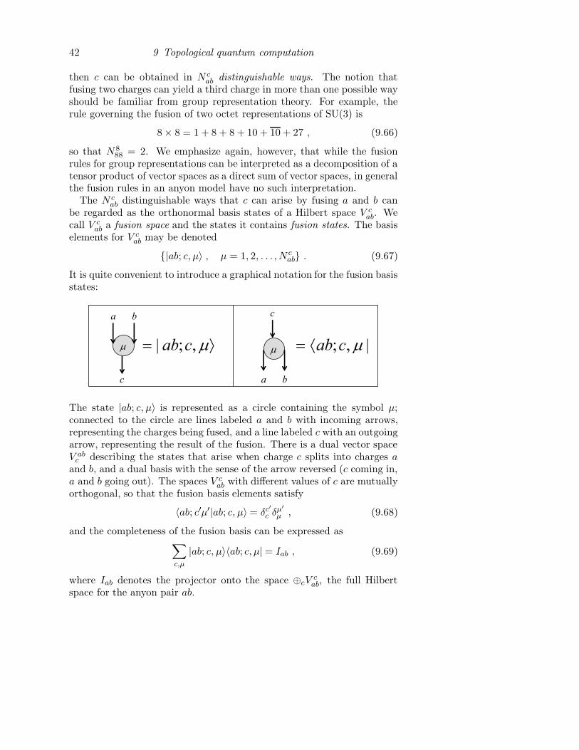
42 9 Topological quantum computation
then c can be obtained in N cab distinguishable ways. The notion that
fusing two charges can yield a third charge in more than one possible wayshould be familiar from group representation theory. For example, therule governing the fusion of two octet representations of SU(3) is
8× 8 = 1 + 8 + 8 + 10 + 10 + 27 , (9.66)
so that N 888 = 2. We emphasize again, however, that while the fusion
rules for group representations can be interpreted as a decomposition of atensor product of vector spaces as a direct sum of vector spaces, in generalthe fusion rules in an anyon model have no such interpretation.
The N cab distinguishable ways that c can arise by fusing a and b can
be regarded as the orthonormal basis states of a Hilbert space V cab. We
call V cab a fusion space and the states it contains fusion states. The basis
elements for V cab may be denoted
{|ab; c, µ〉 , µ = 1, 2, . . . , N cab} . (9.67)
It is quite convenient to introduce a graphical notation for the fusion basisstates:
a
c
b
| ; ,ab c
a
c
b
; , |ab c
The state |ab; c, µ〉 is represented as a circle containing the symbol µ;connected to the circle are lines labeled a and b with incoming arrows,representing the charges being fused, and a line labeled c with an outgoingarrow, representing the result of the fusion. There is a dual vector spaceV ab
c describing the states that arise when charge c splits into charges aand b, and a dual basis with the sense of the arrow reversed (c coming in,a and b going out). The spaces V c
ab with different values of c are mutuallyorthogonal, so that the fusion basis elements satisfy
〈ab; c′µ′|ab; c, µ〉 = δc′
c δµ′
µ , (9.68)
and the completeness of the fusion basis can be expressed as∑
c,µ
|ab; c, µ〉〈ab; c, µ| = Iab , (9.69)
where Iab denotes the projector onto the space ⊕cVcab, the full Hilbert
space for the anyon pair ab.
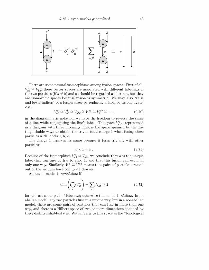
9.12 Anyon models generalized 43
c
a
c´
´
bc
c
a
c
b
a b
a b
,c
There are some natural isomorphisms among fusion spaces. First of all,V c
ab∼= V c
ba; these vector spaces are associated with different labelings ofthe two particles (if a 6= b) and so should be regarded as distinct, but theyare isomorphic spaces because fusion is symmetric. We may also “raiseand lower indices” of a fusion space by replacing a label by its conjugate,e.g.,
V cab
∼= V bac
∼= V 1abc
∼= V bca ,∼= V ab
c∼= · · · ; (9.70)
in the diagrammatic notation, we have the freedom to reverse the senseof a line while conjugating the line’s label. The space V 1
abc, representedas a diagram with three incoming lines, is the space spanned by the dis-tinguishable ways to obtain the trivial total charge 1 when fusing threeparticles with labels a, b, c.
The charge 1 deserves its name because it fuses trivially with otherparticles:
a× 1 = a . (9.71)
Because of the isomorphism V aa1
∼= V 1aa, we conclude that a is the unique
label that can fuse with a to yield 1, and that this fusion can occur inonly one way. Similarly, V a
a1∼= V aa
1 means that pairs of particles createdout of the vacuum have conjugate charges.
An anyon model is nonabelian if
dim
(
⊕
c
V cab
)
=∑
c
N cab ≥ 2 (9.72)
for at least some pair of labels ab; otherwise the model is abelian. In anabelian model, any two particles fuse in a unique way, but in a nonabelianmodel, there are some pairs of particles that can fuse in more than oneway, and there is a Hilbert space of two or more dimensions spanned bythese distinguishable states. We will refer to this space as the “topological
44 9 Topological quantum computation
Hilbert space” of the pair of anyons, to emphasize that this quantuminformation is encoded nonlocally — it is a collective property of thepair, not localized on either particle. Indeed, when the two particles withlabels a and b are far apart, different states in the topological Hilbertspace look identical locally. Therefore, this quantum information is wellhidden, and invulnerable to decoherence due to local interactions withthe environment.
It is for this reason that we propose to use nonabelian anyons in theoperation of a quantum computer. Of course, nonlocally encoded infor-mation is not only hidden from the environment; we are unable to readit ourselves as well. However, with nonabelian anyons, we can have ourcake and eat it too! At the conclusion of a quantum computation, whenwe are ready to perform the readout, we can bring the anyons togetherin pairs and observe the result of this fusion. In fact, it will suffice todistinguish the case where the charge of the composite is c = 1 from thecase c 6= 1 — that is, to distinguish a residual particle (unable to decaybecause of its nontrivial conserved charge) from no particle at all.
Note that for each pair of anyons this topological Hilbert space is finite-dimensional. An anyon model with this property is said to be rational.As in our discussion of the topologically degenerate ground state for anabelian model, anyons in rational nonabelian models always have topo-logical spins that are roots of unity.
9.12.3 Braiding: the R-matrix
When two particles with labels a and b undergo a counterclockwise ex-change, their total charge c is unchanged. Therefore, since the two parti-cles swap positions on the line, the swap induces a natural isomorphismmapping the Hilbert space V c
ba to V cab; this map is the braid operator
R : V cba → V c
ab . (9.73)
If we choose canonical bases {|ba; c, µ〉} and {|ab; c, µ′〉} for these twospaces, R can be expressed as the unitary matrix
R : |ba; c, µ〉 7→∑
µ′
|ab; c, µ′〉 (Rcab)
µ′
µ ; (9.74)
note that R may have a nontrivial action on the fusion states. Whenwe represent the action of R diagrammatically, it is convenient to fix thepositions of the labels a and b on the incoming lines, and twist the linescounterclockwise as they move toward the fusion vertex (µ)— the graphwith twisted lines represents the state in V c
ab obtained by applying R to|ba; c, µ〉, which can be expanded in terms of the canonical basis for V c
ab:
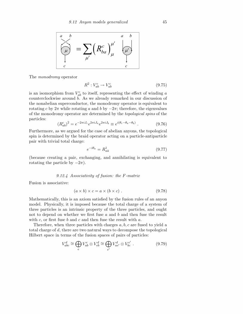
9.12 Anyon models generalized 45
a b
c
a b
c
c
baR
The monodromy operator
R2 : V cab → V c
ab (9.75)
is an isomorphism from V cab to itself, representing the effect of winding a
counterclockwise around b. As we already remarked in our discussion ofthe nonabelian superconductor, the monodromy operator is equivalent torotating c by 2π while rotating a and b by −2π; therefore, the eigenvaluesof the monodromy operator are determined by the topological spins of theparticles:
(Rcab)
2 = e−2πiJce2πiJae2πiJb ≡ ei(θc−θa−θb) . (9.76)
Furthermore, as we argued for the case of abelian anyons, the topologicalspin is determined by the braid operator acting on a particle-antiparticlepair with trivial total charge:
e−iθa = R1aa (9.77)
(because creating a pair, exchanging, and annihilating is equivalent torotating the particle by −2π).
9.12.4 Associativity of fusion: the F -matrix
Fusion is associative:
(a× b)× c = a× (b× c) . (9.78)
Mathematically, this is an axiom satisfied by the fusion rules of an anyonmodel. Physically, it is imposed because the total charge of a system ofthree particles is an intrinsic property of the three particles, and oughtnot to depend on whether we first fuse a and b and then fuse the resultwith c, or first fuse b and c and then fuse the result with a.
Therefore, when three particles with charges a, b, c are fused to yield atotal charge of d, there are two natural ways to decompose the topologicalHilbert space in terms of the fusion spaces of pairs of particles:
V dabc
∼=⊕
e
V eab ⊗ V d
eb∼=⊕
e′
V dae′ ⊗ V e′
bc . (9.79)
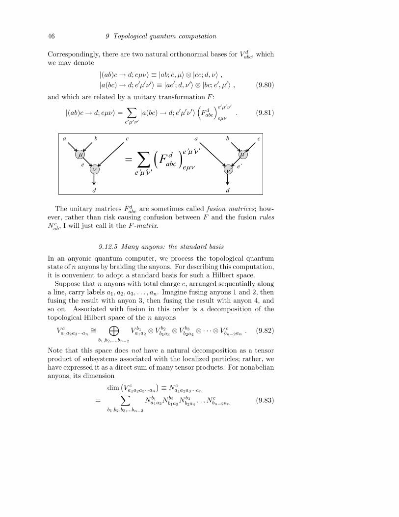
46 9 Topological quantum computation
Correspondingly, there are two natural orthonormal bases for V dabc, which
we may denote
|(ab)c→ d; eµν〉 ≡ |ab; e, µ〉 ⊗ |ec; d, ν〉 ,|a(bc) → d; e′µ′ν′〉 ≡ |ae′; d, ν′〉 ⊗ |bc; e′, µ′〉 , (9.80)
and which are related by a unitary transformation F :
|(ab)c→ d; eµν〉 =∑
e′µ′ν′
|a(bc) → d; e′µ′ν′〉(
F dabc
)e′µ′ν′
eµν. (9.81)
a b c
d
a b c
ed
abce
e
Fe e´
d
The unitary matrices F dabc are sometimes called fusion matrices; how-
ever, rather than risk causing confusion between F and the fusion rules
N cab, I will just call it the F -matrix.
9.12.5 Many anyons: the standard basis
In an anyonic quantum computer, we process the topological quantumstate of n anyons by braiding the anyons. For describing this computation,it is convenient to adopt a standard basis for such a Hilbert space.
Suppose that n anyons with total charge c, arranged sequentially alonga line, carry labels a1, a2, a3, . . . , an. Imagine fusing anyons 1 and 2, thenfusing the result with anyon 3, then fusing the result with anyon 4, andso on. Associated with fusion in this order is a decomposition of thetopological Hilbert space of the n anyons
V ca1a2a3···an
∼=⊕
b1,b2,...,bn−2
V b1a1a2
⊗ V b2b1a3
⊗ V b3b2a4
⊗ · · · ⊗ V cbn−2an
. (9.82)
Note that this space does not have a natural decomposition as a tensorproduct of subsystems associated with the localized particles; rather, wehave expressed it as a direct sum of many tensor products. For nonabeliananyons, its dimension
dim(
V ca1a2a3···an
)
≡ N ca1a2a3···an
=∑
b1,b2,b3,...bn−2
N b1a1a2
N b2b1a3
N b3b2a4
. . .N cbn−2an
(9.83)
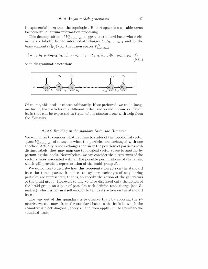
9.12 Anyon models generalized 47
is exponential in n; thus the topological Hilbert space is a suitable arenafor powerful quantum information processing.
This decomposition of V ca1a2a3···an
suggests a standard basis whose ele-ments are labeled by the intermediate charges b1, b2, . . . bn−2 and by the
basis elements {|µj〉} for the fusion spaces Vbj
bj−1,aj+1:
{|a1a2; b1, µ1〉|b1a3; b2, µ2〉 · · · |bn−3an−1; bn−2, µn−2〉|bn−2an; c, µn−1〉} ,(9.84)
or in diagrammatic notation:
1na1
a2
b1
a3
b2
a4
bn-2
an-1
c
an
1 2 2n3
b3
bn-3
Of course, this basis is chosen arbitrarily. If we preferred, we could imag-ine fusing the particles in a different order, and would obtain a differentbasis that can be expressed in terms of our standard one with help fromthe F -matrix.
9.12.6 Braiding in the standard basis: the B-matrix
We would like to consider what happens to states of the topological vectorspace V c
a1a2a3···anof n anyons when the particles are exchanged with one
another. Actually, since exchanges can swap the positions of particles withdistinct labels, they may map one topological vector space to another bypermuting the labels. Nevertheless, we can consider the direct sums of thevector spaces associated with all the possible permutations of the labels,which will provide a representation of the braid group Bn.
We would like to describe how this representation acts on the standardbases for these spaces. It suffices to say how exchanges of neighboringparticles are represented; that is, to specify the action of the generatorsof the braid group. However, so far, we have discussed only the action ofthe braid group on a pair of particles with definite total charge (the R-matrix), which is not in itself enough to tell us its action on the standardbases.
The way out of this quandary is to observe that, by applying the F -matrix, we can move from the standard basis to the basis in which theR-matrix is block diagonal, apply R, and then apply F−1 to return to thestandard basis:
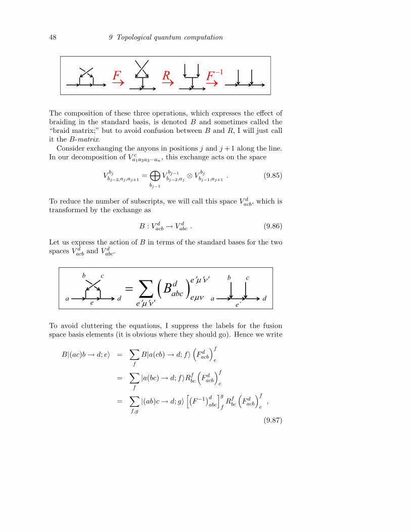
48 9 Topological quantum computation
F R 1F
The composition of these three operations, which expresses the effect ofbraiding in the standard basis, is denoted B and sometimes called the“braid matrix;” but to avoid confusion between B and R, I will just callit the B-matrix.
Consider exchanging the anyons in positions j and j+1 along the line.In our decomposition of V c
a1a2a3···an, this exchange acts on the space
Vbj
bj−2,aj ,aj+1=⊕
bj−1
Vbj−1
bj−2,aj⊗ V
bj
bj−1,aj+1. (9.85)
To reduce the number of subscripts, we will call this space V dacb, which is
transformed by the exchange as
B : V dacb → V d
abc . (9.86)
Let us express the action of B in terms of the standard bases for the twospaces V d
acb and V dabc.
b c
a de
a d
b c
e´
ed
abce
e
B
To avoid cluttering the equations, I suppress the labels for the fusionspace basis elements (it is obvious where they should go). Hence we write
B|(ac)b→ d; e〉 =∑
f
B|a(cb) → d; f〉(
F dacb
)f
e
=∑
f
|a(bc) → d; f〉Rfbc
(
F dacb
)f
e
=∑
f,g
|(ab)c→ d; g〉[
(
F−1)d
abc
]g
fRf
bc
(
F dacb
)f
e,
(9.87)
9.13 Simulating anyons with a quantum circuit 49
or
B : |(ac)b→ d; e〉 7→∑
g
|(ab)c→ d; g〉(
Bdabc
)g
e, (9.88)
where
(
Bdabc
)g
e=∑
f
[
(
F−1)d
abc
]g
fRf
bc
(
F dacb
)f
e. (9.89)
We have expressed the action of the B-matrix in the standard basis interms of the F -matrix and R-matrix, as desired.
Thus, the representation of the braid group realized by n anyons is com-pletely characterized by the F -matrix and the R-matrix. Furthermore, wehave seen that the R matrix also determines the topological spins of theanyons, so that we have actually constructed a representation of a largergroup whose generators include both the exchanges of neighboring parti-cles and 2π rotations of the particles. A good name for this group wouldbe the ribbon group, as its elements are in one-to-one correspondence withthe topological classes of braided ribbons (which can be twisted) ratherthan braided strings; however, mathematicians have already named it“the mapping class group for the sphere with n punctures.”
And with that observation we have completed our description of ananyon model in this general setting. The model is specified by: (1) alabel set, (2) the fusion rules, (3) the R-matrix, and (4) the F matrix.
The mathematical object we have constructed is called a unitary topo-
logical modular functor, and it is closely related to two other objects thathave been much studied: topological quantum field theories in 2+1 space-time dimensions, and conformal field theories in 1+1 spacetime dimen-sions. However, we will just call it an anyon model.
9.13 Simulating anyons with a quantum circuit
A topological quantum computation is executed in three steps:
1. Initialization: Particle-antiparticle pairs c1c1, c2c2, c3c3, . . . , cmcm arecreated. Each pair is of a specified type and has trivial total charge.
2. Processing. The n = 2m particles are guided along trajectories, theirworld lines following a specified braid.
3. Readout. Pairs of neighboring particles are fused together, and it isrecorded whether each pair annihilates fully or not. This record isthe output of the computation.
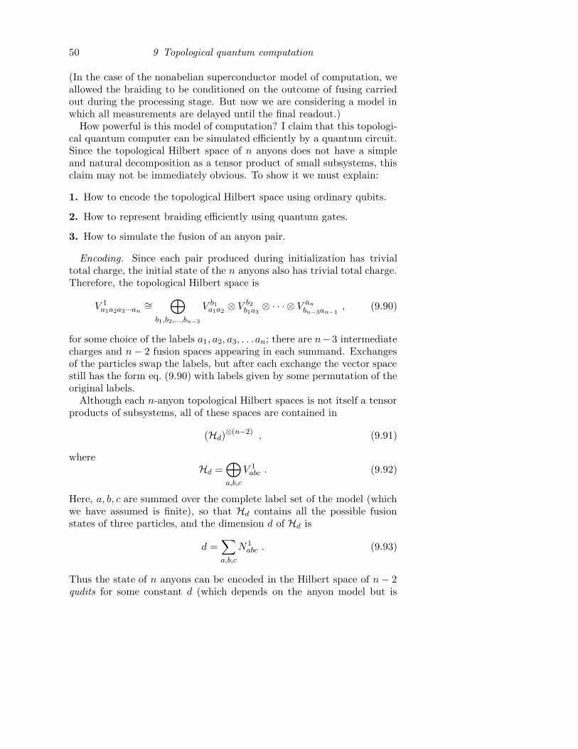
50 9 Topological quantum computation
(In the case of the nonabelian superconductor model of computation, weallowed the braiding to be conditioned on the outcome of fusing carriedout during the processing stage. But now we are considering a model inwhich all measurements are delayed until the final readout.)
How powerful is this model of computation? I claim that this topologi-cal quantum computer can be simulated efficiently by a quantum circuit.Since the topological Hilbert space of n anyons does not have a simpleand natural decomposition as a tensor product of small subsystems, thisclaim may not be immediately obvious. To show it we must explain:
1. How to encode the topological Hilbert space using ordinary qubits.
2. How to represent braiding efficiently using quantum gates.
3. How to simulate the fusion of an anyon pair.
Encoding. Since each pair produced during initialization has trivialtotal charge, the initial state of the n anyons also has trivial total charge.Therefore, the topological Hilbert space is
V 1a1a2a3···an
∼=⊕
b1,b2,...,bn−3
V b1a1a2
⊗ V b2b1a3
⊗ · · · ⊗ V anbn−3an−1
, (9.90)
for some choice of the labels a1, a2, a3, . . .an; there are n−3 intermediatecharges and n− 2 fusion spaces appearing in each summand. Exchangesof the particles swap the labels, but after each exchange the vector spacestill has the form eq. (9.90) with labels given by some permutation of theoriginal labels.
Although each n-anyon topological Hilbert spaces is not itself a tensorproducts of subsystems, all of these spaces are contained in
(Hd)⊗(n−2) , (9.91)
whereHd =
⊕
a,b,c
V 1abc . (9.92)
Here, a, b, c are summed over the complete label set of the model (whichwe have assumed is finite), so that Hd contains all the possible fusionstates of three particles, and the dimension d of Hd is
d =∑
a,b,c
N 1abc . (9.93)
Thus the state of n anyons can be encoded in the Hilbert space of n− 2qudits for some constant d (which depends on the anyon model but is
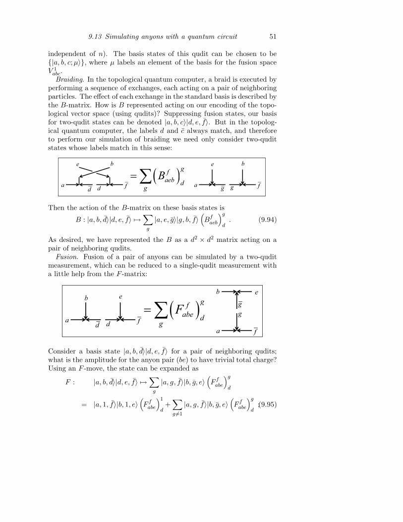
9.13 Simulating anyons with a quantum circuit 51
independent of n). The basis states of this qudit can be chosen to be{|a, b, c;µ〉}, where µ labels an element of the basis for the fusion spaceV 1
abc.Braiding. In the topological quantum computer, a braid is executed by
performing a sequence of exchanges, each acting on a pair of neighboringparticles. The effect of each exchange in the standard basis is described bythe B-matrix. How is B represented acting on our encoding of the topo-logical vector space (using qudits)? Suppressing fusion states, our basisfor two-qudit states can be denoted |a, b, c〉|d, e, f〉. But in the topolog-ical quantum computer, the labels d and c always match, and thereforeto perform our simulation of braiding we need only consider two-quditstates whose labels match in this sense:
gf
aeb dg
Ba fdd
be
a fgg
be
Then the action of the B-matrix on these basis states is
B : |a, b, d〉|d, e, f〉 7→∑
g
|a, e, g〉|g, b, f〉(
Bfaeb
)g
d. (9.94)
As desired, we have represented the B as a d2 × d2 matrix acting on apair of neighboring qudits.
Fusion. Fusion of a pair of anyons can be simulated by a two-quditmeasurement, which can be reduced to a single-qudit measurement witha little help from the F -matrix:
gf
abe dg
Fa fdd
eb
a
e
g
f
b
g
Consider a basis state |a, b, d〉|d, e, f〉 for a pair of neighboring qudits;what is the amplitude for the anyon pair (be) to have trivial total charge?Using an F -move, the state can be expanded as
F : |a, b, d〉|d, e, f〉 7→∑
g
|a, g, f〉|b, g, e〉(
F fabe
)g
d
= |a, 1, f〉|b, 1, e〉(
F fabe
)1
d+∑
g 6=1
|a, g, f〉|b, g, e〉(
F fabe
)g
d;(9.95)
52 9 Topological quantum computation
we have separated the sum over g into the component for which (be) fusesto 1, plus the remainder. After the F -move which (is just a particulartwo-qudit unitary gate), we can sample the probability that (be) fuses to1 by performing a projective measurement of the second qudit in the basis{|b, g, e〉}, and recording whether g = 1.
This completes our demonstration that a quantum circuit can simulateefficiently a topological quantum computer.
9.14 Fibonacci anyons
Now we have established that topological quantum computation is nomore powerful than the quantum circuit model — any problem that canbe solved efficiently by braiding nonabelian anyons can also be solvedefficiently with a quantum circuit. But is it as powerful? Can we simulatea universal quantum computer by braiding anyons? The answer dependson the specific properties of the anyons: some nonabelian anyon modelsare universal, others are not. To find the answer for a particular anyonmodel, we need to understand the properties of the representations of thebraid group that are determined by the F -matrix and R-matrix.
Rather than give a general discussion, we will study one especiallysimple nonabelian anyon model, and demonstrate its computational uni-versality. This model is the very simplest nonabelian model — conformalfield theorists call it the “Yang-Lee model,” but I will call it the “Fibonaccimodel” for reasons that will soon be clear.
In the Fibonacci model there are only two labels — the trivial label,which I will now denote 0, and a single nontrivial label that I will call 1,where 1 = 1. And there is only one nontrivial fusion rule:
1 × 1 = 0 + 1 ; (9.96)
when two anyons are brought together they either annihilate, or fuse tobecome a single anyon. The model is nonabelian because two anyons canfuse in two distinguishable ways.
Consider the standard basis for the Hilbert space V b1n of n anyons, where
each basis element describes a distinguishable way in which the n anyonscould fuse to give total charge b ∈ {0, 1}. If the two anyons furthest tothe left were fused first, the resulting charge could be 0 or 1; this chargecould then fuse with the third anyon, yielding a total charge of 0 or 1,and so on. Finally, the last anyon fuses with the total charge of the firstn − 1 anyons to give the total charge b. Altogether n − 2 intermediatecharges b1, b2, b3, . . . bn−2 appear in this description of the fusion process;thus the corresponding basis element can be designated with a binarystring of length n − 2. If the total charge is 0, the result of fusing the
9.15 Quantum dimension 53
first n− 1 anyons has to be 1, so the basis states are labeled by strings oflength n− 3.
However, not all binary strings are allowed — a 0 must always befollowed by a 1. There cannot be two zeros in a row because when thecharge 0 fuses with 1, a total charge of 1 is the only possible outcome.Otherwise, there is no restriction on the sequence. Therefore, the basisstates are in one-to-one with the binary strings that do not contain twosuccessive 0’s.
Thus the dimensions N 0n ≡ N 0
1n of the topological Hilbert spaces V 01n
obey a simple recursion relation. If the fusion of the first two particlesyields trivial total charge, then the remaining n − 2 particles can fusein N 0
n−2 distinguishable ways, and if the fusion of the first two particlesyields an anyon with nontrivial charge, then that anyon can fuse with theother n− 2 anyons in N 0
n−1 ways; therefore,
N 0n = N 0
n−1 +N 0n−2 . (9.97)
Since N 01 = 0 and N 0
2 = 1, the solution to this recursion relation is
n = 1 2 3 4 5 6 7 8 9 . . .N 0
n = 0 1 1 2 3 5 8 13 21 . . .(9.98)
— the dimensions are Fibonacci numbers (which is why I am calling thismodel the “Fibonacci model”).
The Fibonacci numbers grow with n at a rate N 0n ≈ Cφn, where φ is
the golden mean φ = 12
(
1 +√
5)
≈ 1.618. Because φ governs the rate atwhich the Hilbert space enlarges as anyons are added, we say that d = φis the quantum dimension of the Fibonacci anyon. That this “dimension”is an irrational number illustrates vividly that the topological Hilbertspace has no natural decomposition as a tensor product of subsystems— instead, the topologically encoded quantum information is a collectiveproperty of the n anyons.
9.15 Quantum dimension
We will return shortly to the properties of the Fibonacci model, but firstlet’s explore more deeply the concept of quantum dimension. For a generalanyon model, how should the dimension da of label a be defined? For thispurpose, it is convenient to imagine a physical process in which two aapairs are created (each with trivial total charge); then the particle a fromthe pair on the right fuses with the antiparticle a from the pair on theleft. Do these particles annihilate?
With suitable phase conventions, the amplitude for the annihilationto occur is a real number in the unit interval [0,1]. Let us define this
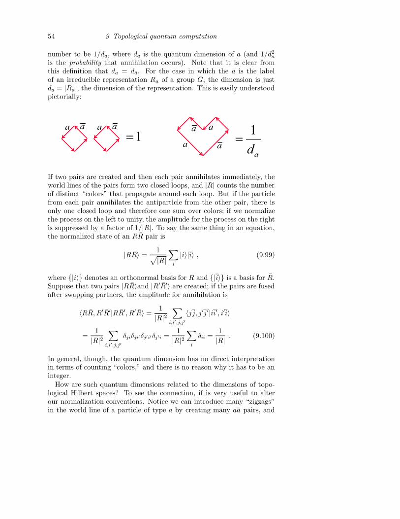
54 9 Topological quantum computation
number to be 1/da, where da is the quantum dimension of a (and 1/d2a
is the probability that annihilation occurs). Note that it is clear fromthis definition that da = da. For the case in which the a is the labelof an irreducible representation Ra of a group G, the dimension is justda = |Ra|, the dimension of the representation. This is easily understoodpictorially:
aa
a a
a a a a1
ad
1
If two pairs are created and then each pair annihilates immediately, theworld lines of the pairs form two closed loops, and |R| counts the numberof distinct “colors” that propagate around each loop. But if the particlefrom each pair annihilates the antiparticle from the other pair, there isonly one closed loop and therefore one sum over colors; if we normalizethe process on the left to unity, the amplitude for the process on the rightis suppressed by a factor of 1/|R|. To say the same thing in an equation,the normalized state of an RR pair is
|RR〉 =1
√
|R|∑
i
|i〉|i〉 , (9.99)
where {|i〉} denotes an orthonormal basis for R and {|i〉} is a basis for R.Suppose that two pairs |RR〉and |R′R′〉 are created; if the pairs are fusedafter swapping partners, the amplitude for annihilation is
〈RR, R′R′|RR′, R′R〉 =1
|R|2∑
i,i′,j,j′
〈jj, j ′j ′|ii′, i′i〉
=1
|R|2∑
i,i′,j,j′
δjiδji′δj′i′δj′i =1
|R|2∑
i
δii =1
|R| . (9.100)
In general, though, the quantum dimension has no direct interpretationin terms of counting “colors,” and there is no reason why it has to be aninteger.
How are such quantum dimensions related to the dimensions of topo-logical Hilbert spaces? To see the connection, if is very useful to alterour normalization conventions. Notice we can introduce many “zigzags”in the world line of a particle of type a by creating many aa pairs, and
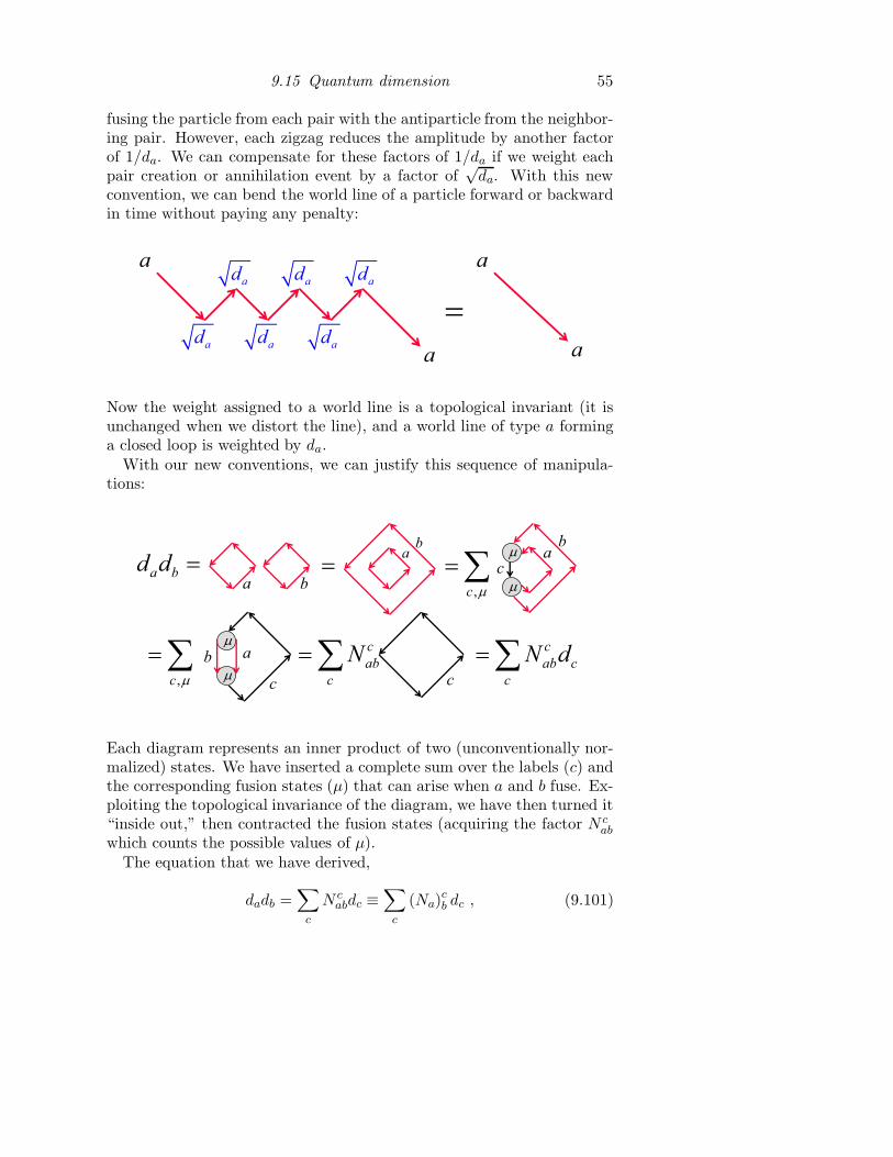
9.15 Quantum dimension 55
fusing the particle from each pair with the antiparticle from the neighbor-ing pair. However, each zigzag reduces the amplitude by another factorof 1/da. We can compensate for these factors of 1/da if we weight eachpair creation or annihilation event by a factor of
√da. With this new
convention, we can bend the world line of a particle forward or backwardin time without paying any penalty:
a
a
ad
ad
ad
ad
ad
ad
a
a
Now the weight assigned to a world line is a topological invariant (it isunchanged when we distort the line), and a world line of type a forminga closed loop is weighted by da.
With our new conventions, we can justify this sequence of manipula-tions:
ab
a b
ab
c c
ab
c
,c
,c
c
ab
c
Nc
ab c
c
N d
a bd d
Each diagram represents an inner product of two (unconventionally nor-malized) states. We have inserted a complete sum over the labels (c) andthe corresponding fusion states (µ) that can arise when a and b fuse. Ex-ploiting the topological invariance of the diagram, we have then turned it“inside out,” then contracted the fusion states (acquiring the factor N c
abwhich counts the possible values of µ).
The equation that we have derived,
dadb =∑
c
N cabdc ≡
∑
c
(Na)cb dc , (9.101)
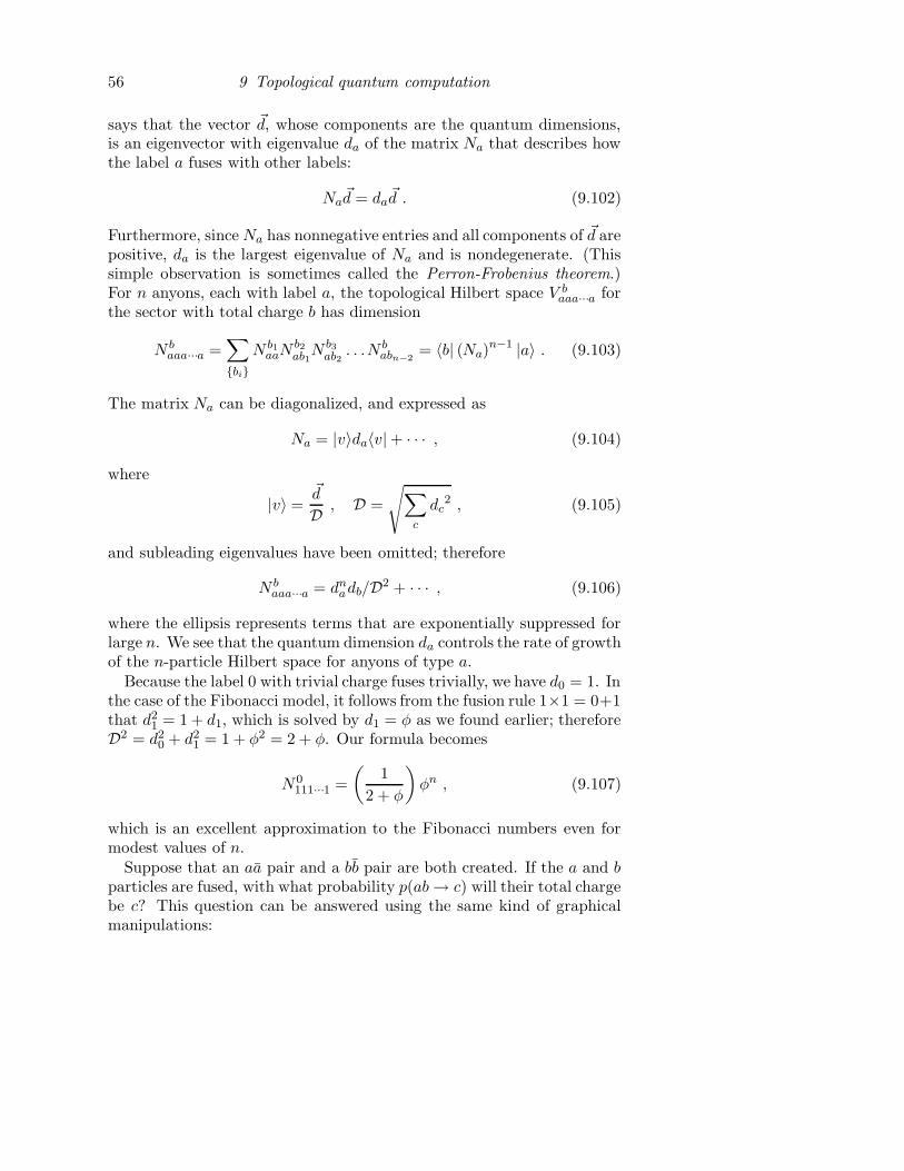
56 9 Topological quantum computation
says that the vector ~d, whose components are the quantum dimensions,is an eigenvector with eigenvalue da of the matrix Na that describes howthe label a fuses with other labels:
Na~d = da
~d . (9.102)
Furthermore, sinceNa has nonnegative entries and all components of ~d arepositive, da is the largest eigenvalue of Na and is nondegenerate. (Thissimple observation is sometimes called the Perron-Frobenius theorem.)For n anyons, each with label a, the topological Hilbert space V b
aaa···a forthe sector with total charge b has dimension
N baaa···a =
∑
{bi}
N b1aaN
b2ab1N b3
ab2. . .N b
abn−2= 〈b| (Na)
n−1 |a〉 . (9.103)
The matrix Na can be diagonalized, and expressed as
Na = |v〉da〈v|+ · · · , (9.104)
where
|v〉 =~d
D , D =
√
∑
c
dc2 , (9.105)
and subleading eigenvalues have been omitted; therefore
N baaa···a = dn
adb/D2 + · · · , (9.106)
where the ellipsis represents terms that are exponentially suppressed forlarge n. We see that the quantum dimension da controls the rate of growthof the n-particle Hilbert space for anyons of type a.
Because the label 0 with trivial charge fuses trivially, we have d0 = 1. Inthe case of the Fibonacci model, it follows from the fusion rule 1×1 = 0+1that d2
1 = 1 + d1, which is solved by d1 = φ as we found earlier; thereforeD2 = d2
0 + d21 = 1 + φ2 = 2 + φ. Our formula becomes
N 0111···1 =
(
1
2 + φ
)
φn , (9.107)
which is an excellent approximation to the Fibonacci numbers even formodest values of n.
Suppose that an aa pair and a bb pair are both created. If the a and bparticles are fused, with what probability p(ab→ c) will their total chargebe c? This question can be answered using the same kind of graphicalmanipulations:
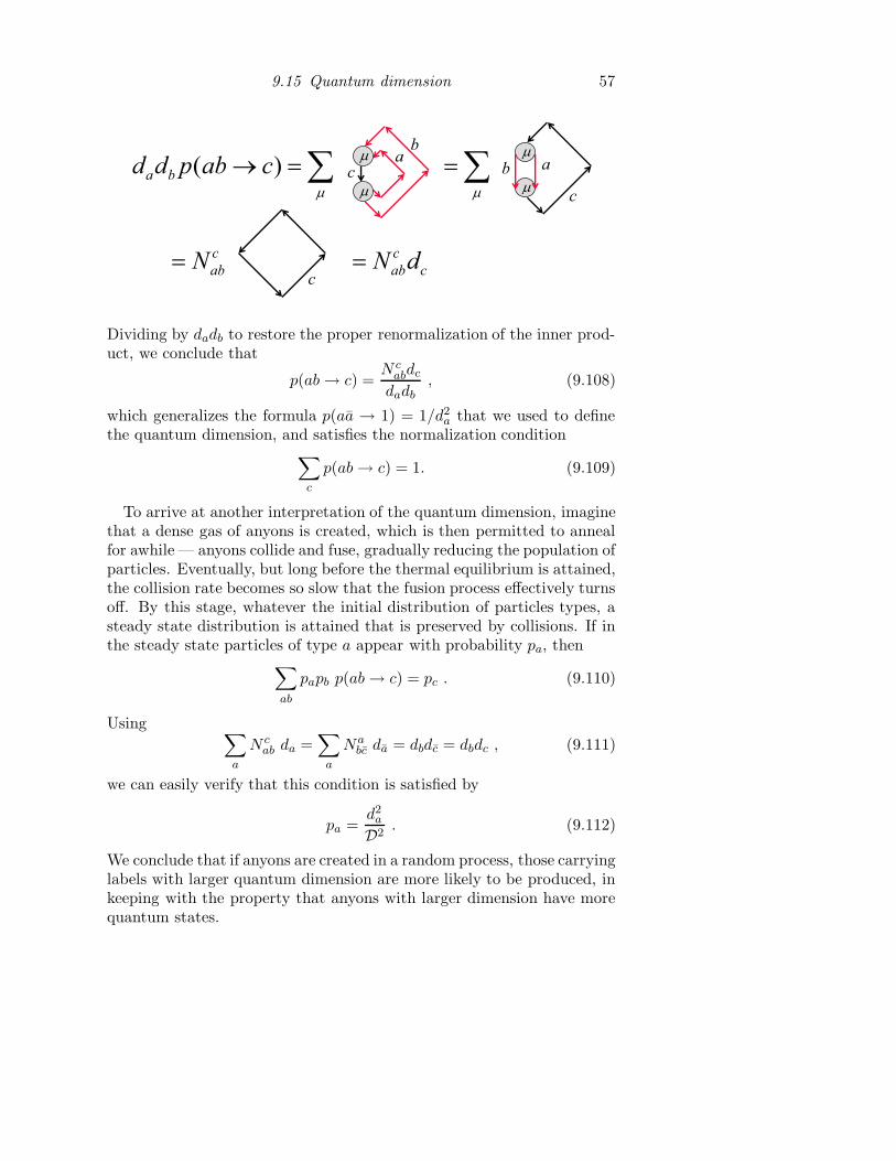
9.15 Quantum dimension 57
a
c
c
c
abNc
ab cN d
ab
c( )a bd d p ab c b
Dividing by dadb to restore the proper renormalization of the inner prod-uct, we conclude that
p(ab→ c) =N c
abdc
dadb, (9.108)
which generalizes the formula p(aa → 1) = 1/d2a that we used to define
the quantum dimension, and satisfies the normalization condition∑
c
p(ab→ c) = 1. (9.109)
To arrive at another interpretation of the quantum dimension, imaginethat a dense gas of anyons is created, which is then permitted to annealfor awhile — anyons collide and fuse, gradually reducing the population ofparticles. Eventually, but long before the thermal equilibrium is attained,the collision rate becomes so slow that the fusion process effectively turnsoff. By this stage, whatever the initial distribution of particles types, asteady state distribution is attained that is preserved by collisions. If inthe steady state particles of type a appear with probability pa, then
∑
ab
papb p(ab→ c) = pc . (9.110)
Using∑
a
N cab da =
∑
a
Nabc da = dbdc = dbdc , (9.111)
we can easily verify that this condition is satisfied by
pa =d2
a
D2. (9.112)
We conclude that if anyons are created in a random process, those carryinglabels with larger quantum dimension are more likely to be produced, inkeeping with the property that anyons with larger dimension have morequantum states.
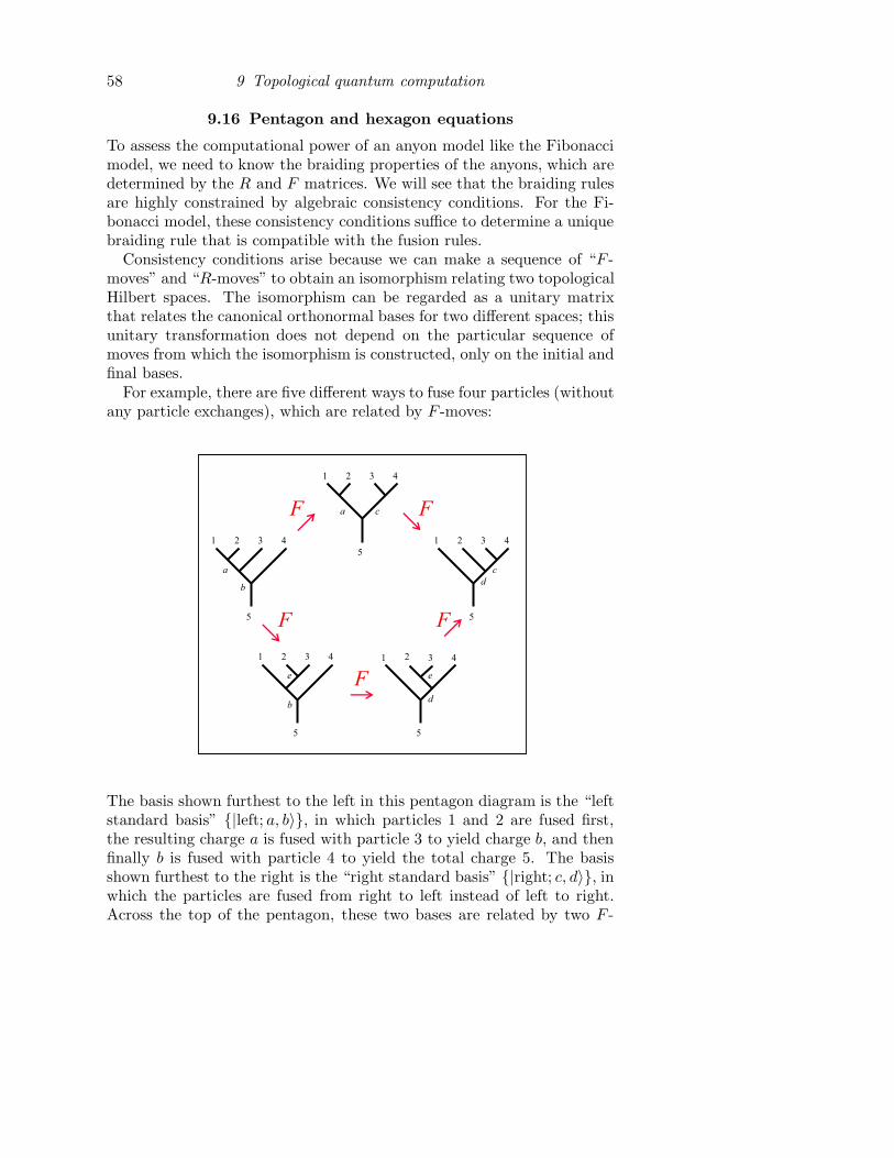
58 9 Topological quantum computation
9.16 Pentagon and hexagon equations
To assess the computational power of an anyon model like the Fibonaccimodel, we need to know the braiding properties of the anyons, which aredetermined by the R and F matrices. We will see that the braiding rulesare highly constrained by algebraic consistency conditions. For the Fi-bonacci model, these consistency conditions suffice to determine a uniquebraiding rule that is compatible with the fusion rules.
Consistency conditions arise because we can make a sequence of “F -moves” and “R-moves” to obtain an isomorphism relating two topologicalHilbert spaces. The isomorphism can be regarded as a unitary matrixthat relates the canonical orthonormal bases for two different spaces; thisunitary transformation does not depend on the particular sequence ofmoves from which the isomorphism is constructed, only on the initial andfinal bases.
For example, there are five different ways to fuse four particles (withoutany particle exchanges), which are related by F -moves:
1 2 3 4
5
a
bd
1 2 3 4
5
c
1 2 3 4
5
1 2 3 4
5
1 2 3 4
5
a c
b
e e
d
F
FF
F F
The basis shown furthest to the left in this pentagon diagram is the “leftstandard basis” {|left; a, b〉}, in which particles 1 and 2 are fused first,the resulting charge a is fused with particle 3 to yield charge b, and thenfinally b is fused with particle 4 to yield the total charge 5. The basisshown furthest to the right is the “right standard basis” {|right; c, d〉}, inwhich the particles are fused from right to left instead of left to right.Across the top of the pentagon, these two bases are related by two F -
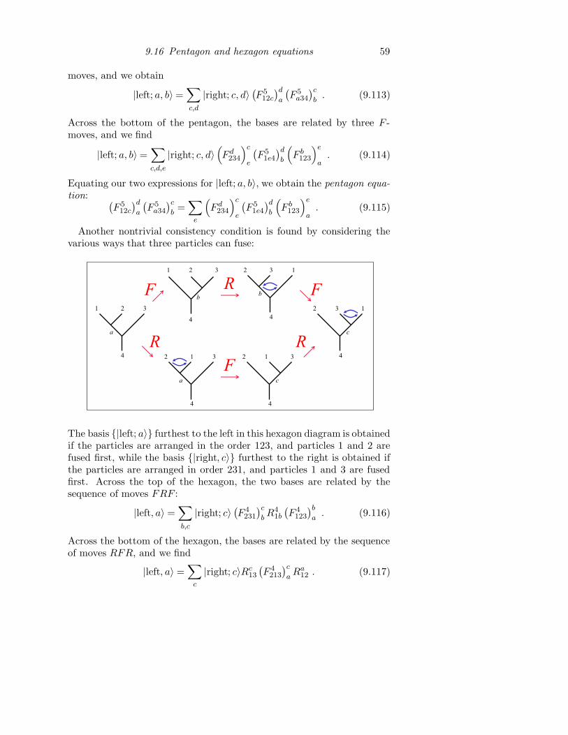
9.16 Pentagon and hexagon equations 59
moves, and we obtain
|left; a, b〉 =∑
c,d
|right; c, d〉(
F 512c
)d
a
(
F 5a34
)c
b. (9.113)
Across the bottom of the pentagon, the bases are related by three F -moves, and we find
|left; a, b〉 =∑
c,d,e
|right; c, d〉(
F d234
)c
e
(
F 51e4
)d
b
(
F b123
)e
a. (9.114)
Equating our two expressions for |left; a, b〉, we obtain the pentagon equa-
tion:(
F 512c
)d
a
(
F 5a34
)c
b=∑
e
(
F d234
)c
e
(
F 51e4
)d
b
(
F b123
)e
a. (9.115)
Another nontrivial consistency condition is found by considering thevarious ways that three particles can fuse:
1 2 3
4
b
1 2 3
4
a
2 3 1
4
b
2 3 1
4
c
2 1 3
4
c
2 1 3
4
a
F R F
F
R R
The basis {|left; a〉} furthest to the left in this hexagon diagram is obtainedif the particles are arranged in the order 123, and particles 1 and 2 arefused first, while the basis {|right, c〉} furthest to the right is obtained ifthe particles are arranged in order 231, and particles 1 and 3 are fusedfirst. Across the top of the hexagon, the two bases are related by thesequence of moves FRF :
|left, a〉 =∑
b,c
|right; c〉(
F 4231
)c
bR4
1b
(
F 4123
)b
a. (9.116)
Across the bottom of the hexagon, the bases are related by the sequenceof moves RFR, and we find
|left, a〉 =∑
c
|right; c〉Rc13
(
F 4213
)c
aRa
12 . (9.117)
60 9 Topological quantum computation
Equating our two expressions for |left; a〉, we obtain the hexagon equation:
Rc13
(
F 4213
)c
aRa
12 =∑
b
(
F 4231
)c
bR4
1b
(
F 4123
)b
a. (9.118)
A beautiful theorem, which I will not prove here, says that there areno further conditions that must be imposed to ensure the consistency ofbraiding and fusing. That is, for any choice of an initial and final basisfor n anyons, all sequences of R-moves and F -moves that take the initialbasis to the final basis yield the same isomorphism, provided that thepentagon equation and hexagon equation are satisfied. This theorem isan instance of the MacLane coherence theorem, a fundamental result incategory theory. The pentagon and hexagon equations together are calledthe Moore-Seiberg polynomial equations — their relevance to physics wasfirst appreciated in studies of (1+1)-dimensional conformal field theoryduring the 1980’s.
A solution to the polynomial equations defines a viable anyon model.Therefore, there is a systematic procedure for constructing anyon models:
1. Choose a set of labels and assume a fusion rule.
2. Solve the polynomial equations for R and F .
If no solutions exist, then the hypothetical fusion rule is incompatible withthe principles of local quantum physics and must be rejected. If there ismore than one solution (not related to one another by any reshuffling ofthe labels, redefinition of bases, etc.), then each distinct solution definesa distinct model with the assumed fusion rule.
To illustrate the procedure, consider the polynomial equations for theFibonacci fusion rule. There are only two F -matrices that arise, whichwe will denote as
F0111 ≡ F0 , F1111 ≡ F1 . (9.119)
F0 is really the 1 × 1 matrix
(F0)ba = δ1aδ
b1 , (9.120)
while F1 is a 2× 2 matrix. The pentagon equation becomes
(Fc)da (Fa)
cb =
∑
e
(Fd)ce (Fe)
db (Fb)
ea . (9.121)
The general solution for F ≡ F1 is
F =
(
τ eiφ√τ
e−iφ√τ −τ
)
, (9.122)
9.17 Simulating a quantum circuit with Fibonacci anyons 61
where eiφ is an arbitrary phase (which we can set to 1 with a suitablephase convention), and τ =
(√5 − 1
)
/2 = φ − 1 ≈ .618, which satisfies
τ2 + τ = 1 . (9.123)
The 2× 2 R-matrix that describes a counterclockwise exchange of twoFibonacci anyons has two eigenvalues — R0 for the case where the totalcharge of the pair of anyons is trivial, and R1 for the case where the totalcharge is nontrivial. The hexagon equation becomes
Rc (F )caR
a = (F )c0 (F )0a + (F )c
1R1 (F )1a . (9.124)
Using the expression for F found by solving the pentagon equation, wecan solve the hexagon equation for R, finding
R =
(
e4πi/5 0
0 −e2πi/5
)
, F =
(
τ√τ√
τ −τ
)
. (9.125)
The only other solution is the complex conjugate of this one; this secondsolution really describes the same model, but with clockwise and coun-terclockwise braiding interchanged. Therefore, an anyon model with theFibonacci fusion rule really does exist, and it is essentially unique.
9.17 Simulating a quantum circuit with Fibonacci anyons
Now we know enough to address whether a universal quantum computercan be simulated using Fibonacci anyons. We need to explain how qubitscan be encoded with anyons, and how a universal set of quantum gatescan be realized.
First we note that the Hilbert space V 04 ≡ V 0
1111 has dimension N 04 = 2;
therefore a qubit can be encoded by four anyons with trivial total charge.The anyons are lined up in order 1234, numbered from left to right; in thestandard basis state |0〉, anyons number 1 and number 2 fuse to yield totalcharge 0, while in the standard basis state |1〉, anyons 1 and 2 fuse to yieldtotal charge 1. Acting on this standard basis, the braid group generatorσ1 (counterclockwise exchange of particles 1 and 2) is represented by
σ1 7→ R =
(
e4πi/5 0
0 −e2πi/5
)
, (9.126)
while the generator σ2 is represented by
σ2 7→ B = F−1RF , F =
(
τ√τ√
τ −τ
)
. (9.127)
62 9 Topological quantum computation
These matrices generate a representation of the braid group B3 on threestrands whose image is dense in SU(2). Indeed, R and B generate Z10
subgroups of U(2), about two distinct axes, and there is no finite sub-group of U(2) that contains both of these subgroups — therefore, therepresentation closes on the group containing all elements of U(2) withdeterminant equal to a 10th root of unity. Similarly, for n anyons withtrivial total charge, the image of the representation of the braid group isdense in SU(N 0
n).To simulate a quantum circuit acting on n qubits, altogether 4n anyons
are used. We have just seen that by braiding within each cluster of fouranyons, arbitrary single-qubit gates can be realized. To complete a uni-versal set, we will need two-qubit gates as well. But two neighboringqubits are encoded by eight anyons, and exchanges of these anyons gen-erate a representation of B8 whose image is dense in SU(N 0
8 )= SU(13),which of course includes the SU(4) that acts on the two encoded qubits.Therefore, each gate in a universal set can be simulated with arbitraryaccuracy by some finite braid.
Since we can braid clockwise as well as counterclockwise, the inverseof each exchange gate is also in our repertoire. Therefore, we can ap-ply the Solovay-Kitaev theorem to conclude that the universal gates ofthe circuit model can be simulated to accuracy ε with braids of lengthpoly (log(1/ε)). It follows that an ideal quantum circuit with L gatesacting on all together n qubits can be simulated to fixed accuracy using4n anyons and a braid of length O(L · poly(log(L)). As desired, we haveshown that a universal quantum computer can be simulated efficientlywith Fibonacci anyons. Note that, in contrast to the simulation usingthe nonabelian superconductor model, no intermediate measurements areneeded to realize the universal gates.
In the analysis above, we have assumed that there are no errors inthe simulation other than those limiting the accuracy of the Solovay-Kitaev approximation to the ideal gates. It is therefore implicit that thetemperature is small enough compared to the energy gap of the modelthat thermally excited anyons are too rare to cause trouble, that theanyons are kept far enough apart from one another that uncontrolledexchange of charge can be neglected, and in general that errors in thetopological quantum computation are unimportant. If the error rate issmall but not completely negligible, then the standard theory of quantumfault tolerance can be invoked to boost the accuracy of the simulation asneeded, at an additional overhead cost polylogarithmic in L. The fault-tolerant procedure should include a method for controlling the “leakage”of the encoded qubits — that is, to prevent the drift of the clusters offour qubits from the two-dimensional computational space V 0
4 to its three-dimensional orthogonal complement V 1
4 .
9.18 Epilogue 63
9.18 Epilogue
That is as far as I got in class. I will mention briefly here a few othertopics that I might have covered if I had not run out of time.
9.18.1 Chern-Simons theory
We have discussed how anyon models can be constructed through a brute-force solution to the polynomial equations. This method is foolproof,but in practice models are often constructed using other, more efficientmethods. Indeed, most of the known anyon models have been found asinstances of Chern-Simons theory.
The fusion rules of a Chern-Simons theory are a truncated version of thefusion rules for irreducible representations of a Lie group. For example,associated with the group SU(2) there is a tower of Chern-Simons theoriesindexed by a positive integer k. For SU(2), the irreducible representationscarry labels j = 0, 1
2 , 1,32 , 2,
52 , . . . , and the fusion rules have the form
j1 × j2 =
j1+j2∑
j=|j2−j1|
j . (9.128)
In the Chern-Simons theory denoted SU(2)k, the half-integer labels arelimited to j ≤ k/2, and the label j is contained in j1×j2 only if j1+j2+j ≤k.
For example, the SU(2)1 model is abelian, and the nontrivial fusionrules of the SU(2)2 model are
12 × 1
2 = 0 + 1 ,
12 × 1 =
1
2,
1 × 1 = 0 . (9.129)
Therefore, the label 12 has quantum dimension d1/2 =
√2, and the topo-
logical Hilbert space of 2m such anyons with total charge 0 has dimension
N 0
(12)
2m = 2m−1 . (9.130)
The polynomial equations for these fusion rules have multiple solutions(only one of which describes the braiding properties of the SU(2)2 model),but none of the resulting models have computationally universal braidingrules. The space V 0
12
12
12
12
is two-dimensional, and the 2 × 2 matrices F ≡F 1
212
12
12
and R ≡ R 12
12
are, up to overall phases and complex conjugation,
F = H =1√2
(
1 11 −1
)
, R = P =
(
1 00 i
)
. (9.131)
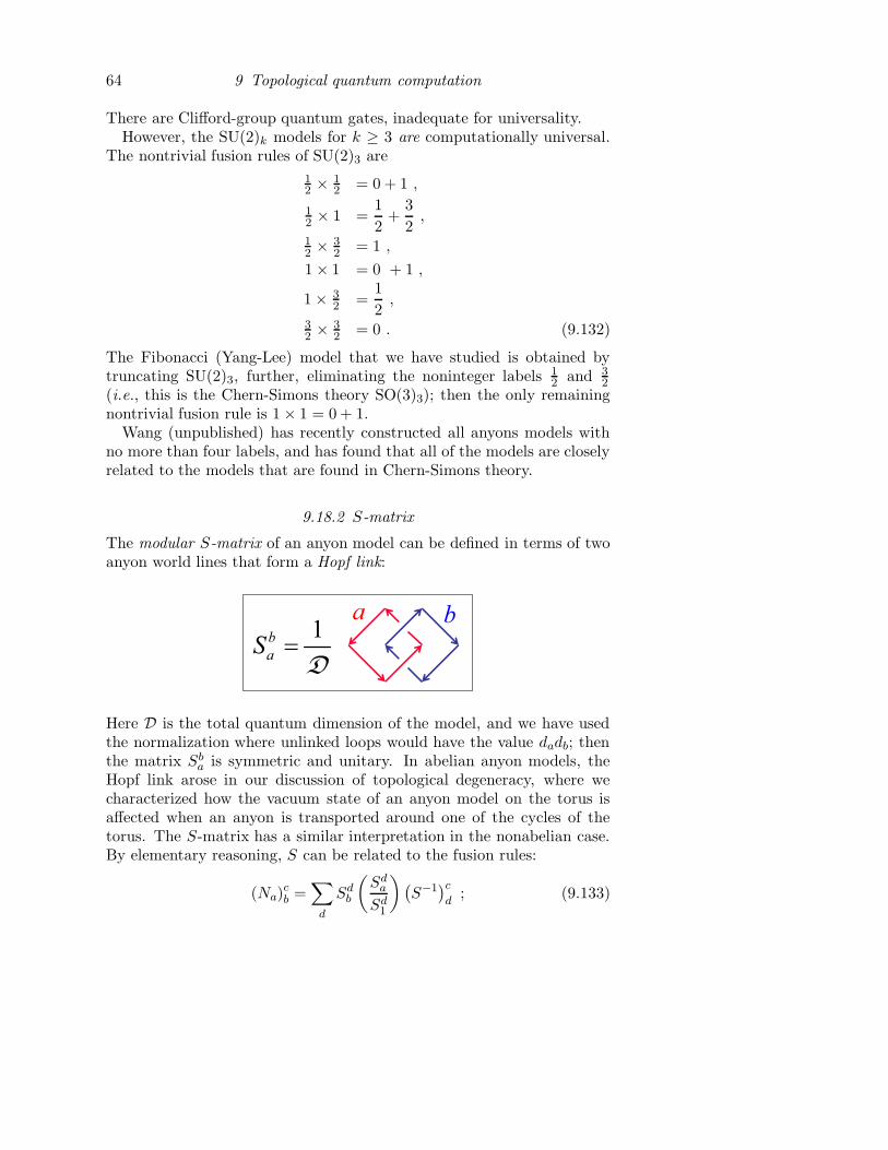
64 9 Topological quantum computation
There are Clifford-group quantum gates, inadequate for universality.However, the SU(2)k models for k ≥ 3 are computationally universal.
The nontrivial fusion rules of SU(2)3 are
12 × 1
2 = 0 + 1 ,
12 × 1 =
1
2+
3
2,
12 × 3
2 = 1 ,
1 × 1 = 0 + 1 ,
1 × 32 =
1
2,
32 × 3
2 = 0 . (9.132)
The Fibonacci (Yang-Lee) model that we have studied is obtained bytruncating SU(2)3, further, eliminating the noninteger labels 1
2 and 32
(i.e., this is the Chern-Simons theory SO(3)3); then the only remainingnontrivial fusion rule is 1 × 1 = 0 + 1.
Wang (unpublished) has recently constructed all anyons models withno more than four labels, and has found that all of the models are closelyrelated to the models that are found in Chern-Simons theory.
9.18.2 S-matrix
The modular S-matrix of an anyon model can be defined in terms of twoanyon world lines that form a Hopf link:
1b
aS
D
ba
Here D is the total quantum dimension of the model, and we have usedthe normalization where unlinked loops would have the value dadb; thenthe matrix Sb
a is symmetric and unitary. In abelian anyon models, theHopf link arose in our discussion of topological degeneracy, where wecharacterized how the vacuum state of an anyon model on the torus isaffected when an anyon is transported around one of the cycles of thetorus. The S-matrix has a similar interpretation in the nonabelian case.By elementary reasoning, S can be related to the fusion rules:
(Na)cb =
∑
d
Sdb
(
Sda
Sd1
)
(
S−1)c
d; (9.133)
9.19 Bibliographical notes 65
that is, the S-matrix simulaneously diagonalizes all the matrices {Na}(the Verlinde relation). Note that it follows from the definition that Sa
1 =da/D.
9.18.3 Edge excitations
In our formulation of anyon models, we have discussed the fusing andbraiding of particles in the two-dimensional bulk. But there is anotheraspect of the physics of two-dimensional media that we have not yet dis-cussed, the properties of the one-dimensional edge of the sample. Typi-cally, if a two-dimensional system supports anyons in the bulk, there arealso chiral massless excitations that propagate along the one-dimensionaledge. At nonzero temperature T , there is an energy flux along the edgegiven by the expression
J =π
12c−T
2 ; (9.134)
here the constant c−, called the chiral central charge of the edge, is auniversal property that is unaffected by small changes in the underlyingHamiltonian of the system.
While this chiral central charge is an intrinsic property of the two-dimensional medium, the properties of the anyons in the bulk do notdetermine it completely; rather we have
1
D∑
a
d2ae
2πiJa = e(2πi/8)c− , (9.135)
where the sum is over the complete label set of the anyon model, ande2πiJa = R1
aa is the topological spin of the label a. This expression re-lates the quantity c−, characteristic of the edge theory, to the quantumdimensions and topological spins of the bulk theory, but determines c−only modulo 8. Therefore, at least in principle, there can be multiple edgetheories corresponding to a single theory of anyons in the bulk.
9.19 Bibliographical notes
Some of the pioneering papers on the theory of anyons are reprinted in[1].
What I have called the “nonabelian superconductor” model is oftenreferred to in the literature as the “quantum double,” and is studiedusing the representation theory of Hopf algebras. For a review see [2].
That nonabelian anyons can be used for fault-tolerant quantum com-puting was first suggested in [3]. This paper also discusses the toric code,and related lattice models that have nonabelian phases. A particular real-ization of universal quantum computation in a nonabelian superconductor
66 9 Topological quantum computation
was discussed in [4, 5]. My discussion of the universal gate set is basedon [6], where more general models are also discussed. Other schemes,that make more extensive use of electric charges and that are universalfor smaller groups (like S3) are described in [7].
Diagrammatic methods, like those I used in the discussion of the quan-tum dimension, are extensively applied to derive properties of anyons in[8]. The role of the polynomial equations (pentagon and hexagon equa-tions) in (1+1)-dimensional conformal field theory is discussed in [9].
Simulation of anyons using a quantum circuit is discussed in [10]. Simu-lation of a universal quantum computer using the anyons of the SU(2)k=3
Chern-Simons theory is discussed in [11]. That the Yang-Lee model isalso universal was pointed out in [12].
I did not discuss physical implementations in my lectures, but I list afew relevant references here anyway: Ideas about realizing abelian andnonabelian anyons using superconducting Josephson-junction arrays arediscussed in [13]. A spin model with nearest-neighbor interactions thathas nonabelian anyons (though not ones that are computationally univer-sal) is proposed and solved in [14], and a proposal for realizing this modelusing cold atoms trapped in an optical lattice is described in [15]. Someideas about realizing the (computationally universal) SU(2)k=3 model ina system of interacting electrons are discussed in [16].
Much of my understanding of the theory of computing with nonabeliananyons was derived from many helpful discussions with Alexei Kitaev.
References
[1] F. Wilczek, Fractional statistics and anyon superconductivity (World Scien-tific, Singapore, 1990).
[2] M. de Wild Propitius and F. A. Bais, “Discrete gauge theories,” arXiv:hep-th/9511201 (1995).
[3] A. Yu. Kitaev, “Fault-tolerant quantum computation by anyons,” AnnalsPhys. 303, 2-30 (2003), arXiv: quant-ph/9707021.
[4] R. W. Ogburn and H. Preskill, “Topological quantum computation,” Lect.Notes in Comp. Sci. 1509, 341-356 (1999).
[5] J. Preskill, “Fault-tolerant quantum computation,” arXiv: quant-ph/9712048 (1997).
[6] C. Mochon, “Anyons from non-solvable finite groups are sufficient for uni-versal quantum computation” Phys. Rev. A 67, 022315 (2003), quant-ph/0206128.
[7] C. Mochon, “Anyon computers with smaller groups,” Phys. Rev. A 69,032306 (2004), arXiv: quant-ph/0306063.
[8] J. Frohlich and F. Gabbiani, “Braid statistics in local quantum theory,”Rev. Math. Phys. 2:3, 251–353 (1990).
[9] G. Moore and N. Seiberg, “Classical and quantum conformal field theory,”Comm. Math. Phys. 123, 171–254 (1989).
[10] M. H. Freedman, A. Kitaev, and Z. Wang, “Simulation of topological fieldtheories by quantum computers,” Comm. Math. Phys. 227, 587-603 (2002),arXiv: quant-ph/0001071.
[11] M. H. Freedman, M. Larsen, and Z. Wang, “A modular functor which isuniversal for quantum computation,” arXiv: quant-ph/0001108 (2000).
[12] G. Kuperberg, unpublished.
[13] B. Doucot, L. B. Ioffe, and J. Vidal, “Discrete non-Abelian gauge theo-ries in two-dimensional lattices and their realizations in Josephson-junctionarrays,” Phys. Rev. B 69, 214501 (2004), arXiv: cond-mat/0302104.
67
68 References
[14] A. Kitaev, “Anyons in a spin model on the honeycomb lattice,” unpublished.
[15] L.-M. Duan, E. Demler, and M. D. Lukin, “Controlling spin exchange inter-actions of ultracold atoms in optical lattices,” Phys. Rev. Lett. 91, 090402(2003), arXiv: cond-mat/0210564.
[16] M. Freedman, C. Nayak, K. Shtengel, K. Walker, and Zhenghan Wang, “Aclass of P, T -invariant topological phases of interacting electrons,” cond-mat/0307511 (2003).

![Anyons in an exactly solved model and beyond …arXiv:cond-mat/0506438v3 [cond-mat.mes-hall] 1 Jan 2008 Anyons in an exactly solved model and beyond Alexei Kitaev California Institute](https://static.fdocuments.us/doc/165x107/5e385f7af119de5653077d70/anyons-in-an-exactly-solved-model-and-beyond-arxivcond-mat0506438v3-cond-matmes-hall.jpg)


![arXiv:0707.1889v2 [cond-mat.str-el] 28 Mar 2008 · 2008-03-28 · arXiv:0707.1889v2 [cond-mat.str-el] 28 Mar 2008 Non-Abelian Anyons and Topological Quantum Computation Chetan Nayak1,2,](https://static.fdocuments.us/doc/165x107/5fb56b7aaee294327c71fcb9/arxiv07071889v2-cond-matstr-el-28-mar-2008-2008-03-28-arxiv07071889v2-cond-matstr-el.jpg)