y Christos-Alexandros Psomas z - arXiv · The Sample Complexity of Auctions with Side Information...

The Sample Complexity of Auctions with Side Information

Nikhil R. Devanur ∗ Zhiyi Huang † Christos-Alexandros Psomas ‡

Abstract

Traditionally, the Bayesian optimal auction design problem has been considered either whenthe bidder values are i.i.d, or when each bidder is individually identifiable via her value dis-tribution. The latter is a reasonable approach when the bidders can be classified into a fewcategories, but there are many instances where the classification of bidders is a continuum. Forexample, the classification of the bidders may be based on their annual income, their propensityto buy an item based on past behavior, or in the case of ad auctions, the click through rateof their ads. We introduce an alternate model that captures this aspect, where bidders are apriori identical, but can be distinguished based (only) on some side information the auctioneerobtains at the time of the auction.

We extend the sample complexity approach of Dhangwatnotai et al. [7] and Cole and Rough-garden [6] to this model and obtain almost matching upper and lower bounds. As an aside, weobtain a revenue monotonicity lemma which may be of independent interest. We also show howto use Empirical Risk Minimization techniques to improve the sample complexity bound of Coleand Roughgarden [6] for the non-identical but independent value distribution case.

∗Microsoft Research†University of Hong Kong‡UC Berkeley

arX

iv:1

511.

0229

6v4

[cs

.GT

] 1

4 Ju

n 20

17

1 Introduction

Myerson’s [16] theory of optimal auctions has been (deservingly) much celebrated. When bidders’values are independently and identically distributed (iid), it gives the beautiful conclusion that asecond price auction with a reserve price is revenue optimal among all incentive compatible andindividually rational auction formats. When the bidders are distinguishable, via a distinct valuedistribution for each bidder, the theory still characterizes the optimal auction, even though it isnot as simple as in the iid case.

The non-identical but independent distribution (non-iid) model could be applicable in practicewhen bidders can be classified into a few different categories, and market research provides adistribution for each of these. The starting point for this paper is the observation that often,the classification of bidders is a continuum, rather than discrete. Suppose for instance that theauctioneer knows the incomes of all the bidders. It is reasonable to assume that bidders withhigher incomes in general have higher valuations and thus use this information in the auctiondesign. Similarly the auctioneer could use knowledge about the bidders’ past purchasing behaviorto distinguish between them. The same observation applies if you have a seller who simply offersan item at a posted price, which is equivalent to an “auction with a single agent”.

In this paper, we propose a model where the side information that can be used to distinguishbetween the bidders comes from a continuum. A priori, bidders are identical: all bidders drawtwo numbers, a value and a “signal”, iid from a joint probability distribution. The signal is a realnumber in [0, 1] that captures the side information that the auctioneer has about the bidder. Weassume that the marginal distribution of the values conditioned on the signal is monotone in thesignal, in the order of first order stochastic dominance.

Even when the bidder categories are discrete,1 it is more natural that there is a distributionover categories. If bidders from some categories appear more often than others, then it is moreimportant that the auction does the right thing for these categories. Also, it is more natural thatthis is represented in the samples as well, so the number of samples for each category would bedifferent if you collected samples at random from the population. Further, it is very common tohave a total ordering on the categories, where bidders in the higher categories have higher values,and this structure could be exploited. (See Leonardi and Roughgarden [14], Bhattacharya et al. [3]for example.) Our model incorporates these aspects of the real world and hence is a better fit formany practical applications.

Ad Auctions Billions of auctions are run each day for ads, for search and display advertising.Setting reserve prices in these auctions has received a lot of attention [10, 21, 18, 17], and has beenone of the prime applications of Myerson’s theory [17]. Common techniques in practice include usingmachine learning algorithms, to map features of an auction into one of few categories, and use thecorresponding reserve price. These settings might benefit from a “continuous categorization”,2

where the machine learning algorithms map the features to a real number instead. This wouldcorrespond exactly to our model, with this number as the signal. One such number might alreadybe calculated: it has been observed that the click-through rates are positively correlated withbids/values, so these rates can be used as the signals. Such a phenomenon, of using the click-throughrates to differentially charge bidders already happens currently, although indirectly, through thepractice of “squashing” [13].

1Note that our model can handle discrete categories as well, where the signal is just an encoding of the categories.2The techniques used are mostly from continuous optimization, with extra effort required to map these into discrete

categories.

1

Sample Complexity When the joint probability distribution over values and signals is com-pletely known to the auctioneer, Myerson’s theory readily extends to this case: simply run Myer-son’s auction on the conditional value distributions. The question that we consider in this paperis that of sample complexity: how many samples from the distribution are necessary/sufficient toapproximate the optimal auction?

The sample complexity approach to revenue maximization [7, 6, 12, 15] assumes that we aregiven access to samples from the value distribution and measures the number of samples that arenecessary/sufficient to approximate the optimal auction. This study is motivated by the observationthat the source of priors is really past data, both in principle and in practice [17]. The goal hasbeen to put such practices on a sound theoretical footing, by identifying principled approaches andprecisely quantifying the value of data.

Dhangwatnotai et al. [7] initiated this line of research, by giving almost tight bounds for the caseof a single agent, which was later extended to multiple agents (with non-identical but independentregular distributions) by Cole and Roughgarden [6]. In this paper we improve the upper bound intheir [6] model, which we’ll refer to as the non-iid model, from O(n10ε−7) to O(nε−4). A detaileddiscussion of the upper and lower bounds for different variants, and comparisons with other relatedwork such as Morgenstern and Roughgarden [15], Huang et al. [12] is in Section 2.2.

Techniques The improvement in the sample complexity upper bounds in the non-iid modelcomes from taking a PAC learning/Empirical Risk Minimization (ERM) approach. We first showhow to discretize the value space while losing only an O(ε) fraction of the revenue. This thenallows us to bound the number of different mechanisms that we need to consider. Then we use aconcentration inequality to argue that for each mechanism in this class, its revenue on the sampleclosely approximates its actual revenue from the distribution. Thus, using the best auction on thesample suffices.

As an important part of this approach we prove a new concentration inequality that might beof independent interest. Consider the revenue of a mechanism with n agents in the non-iid model.Consider a matrix of values, each drawn independently, with the values in column i drawn from thedistribution corresponding to agent i. Chernoff bounds tells us that the revenue of the mechanismaveraged over the row vectors of this matrix is close to its expected revenue w.r.t the distribution.Our concentration inequality gives the same conclusion for the revenue of the mechanism w.r.t.the product of the empirical distributions over each column of the matrix. Due to this, instead offinding the optimal auction for a correlated distribution, it is sufficient to find the optimal auctionfor a product distribution, a computationally easy task.

The model with side information, which we’ll refer to as the Signals model, presents thefollowing new conceptually important challenge: we cannot rely on having seen samples with exactlythe same signals as the participants in the auction. This requires us to be able to interpolateusing samples from different distributions, rather than use samples from the same distributionas in the non-iid model.3 We do this by using just the right number of signals in the sampleimmediately below the actual signal of an agent, and run a version of the Empirical Myerson auction.The approximation factor is proved via a careful charging argument. Our bounds depend on thefollowing quantity: suppose that an ε fraction of the revenue is contributed by the top q(ε) fraction(in probability mass) of signals. For instance, when there is a single agent, O(log(1

ε )q(ε)−1ε−3)

samples are sufficient and Ω(log( 1q(ε))ε−4) are necessary.4

3This introduces additional difficulties such as that convex combinations of regular distributions are not regular,e.g., see Sivan and Syrgkanis [20].

4This is not a contradiction since q(ε) is always at most ε and x log(1/x) is a monotone increasing function for

2

An essential component of interpolating from different distributions is revenue monotonicity.Consider the optimal auction M for a given product distribution D. If M is run on values thatcome from a higher (component wise first order stochastic dominating) distribution, does it get ahigher revenue? Surprisingly, as far as we know, this fundamental question about optimal auctionswas unanswered prior to this paper; we resolve this in the affirmative. Another application of thisproperty is in devising mechanisms when only certain statistics (such as the medians) of the valuedistributions are known (Azar et al. [1]).5 The proof of this property is indirect;6 we first reducethis to a weaker property, namely monotonicity of the optimum revenue (over a larger class ofdistributions), using Sion’s minimax theorem [19]. We then show monotonicity of the optimumrevenue using convexity of the optimum revenue in the space of distributions.

For the lower bounds, we extend the instances used by Huang et al. [12], by packing scaledcopies of them among the conditional distributions for different signals. We can show that in orderto achieve high revenue overall it is necessary to achieve high revenue in most of the conditionals.Moreover, in order to get good revenue from any conditional (even with exact knowledge of therest) a reduction to classification shows that ε−3 samples are necessary; the bound follows.

Extensions Our results can be extended to more general single parameter families of auctionenvironments. We can also get better upper bounds for the case of n agents when we are requiredto optimize over a smaller class of auctions, such as VCG with reserve prices. We discuss theseextensions in Section 6.

Other Related Work Elkind [9] also considers a learning question very similar to the samplecomplexity line of work [7, 6, 12, 15], in the presence of an oracle that returns the expected profitof a given mechanism, for distributions with finite support. This line of work is also close in spiritto Balcan et al. [2], who use PAC learning techniques to design prior-free auctions in a generalsetting. In fact, Huang et al. [12] note that the results of Balcan et al. [2] can be used to deducesample complexity bounds in the iid model. In addition to the lower bound of Ω(ε−3) for regulardistributions, Huang et al. [12] also show tight bounds of Θ(ε−3/2) for MHR distributions. Whileall these results are for single parameter environments, Dughmi et al. [8] show an exponential lowerbound for a multi parameter setting.

Future Directions Much of the auction theory since Myerson, in particular in the algorithmicgame theory literature, is devoted to cases where the distributions are not known. One can askseveral “simple vs. optimal” questions in the side information setting, such as an extension of thefamous result of Bulow and Klemperer [4]: how much does the market size have to increase for

small enough x.5A natural mechanism to consider in such a setting is the optimal mechanism w.r.t. the minimal distribution with

the given statistics. Given the value of the median µ, the distribution which is 0 or µ with probability 12

each is firstorder stochastically dominated by all other distributions with median µ.

6Direct approaches seem to fail here. Consider the following example, where increasing one component distributionfirst increases the revenue, and then increasing another component decreases the revenue (all w.r.t. an optimalmechanism for the original distribution). There are two bidders: bidder 1 has value distribution U [0, 100] and bidder2 has distribution U [0, 1]. The virtual value functions are φ1 = 2v − 100 and φ2 = 2v − 1 respectively. If bidder 1’sdistribution is replaced by U [50, 100], the revenue strictly increases, since the probability of allocating the item toher (for a high price) increases. In fact bidder 1 always gets the item, except when she has a value in [50, 50.5] andbidder 2 has a value in [0.5, 1] with higher virtual value. When this occurs the item is sold to bidder 2 for a low price.The probability of this event strictly increases when bidder 2’s distribution is replaced with a point mass at 1, andthus the revenue slightly decreases. The net effect is still an increase in the revenue, as guaranteed by our theorem.This also shows that revenue monotonicity is not true w.r.t any mechanism.

3

the Vickrey auction to outperform the optimal auction. Another interesting direction is to ask forthe design of a prior-independent mechanism in this model, which might be easier than a similarattempt in the prior-free setting by Leonardi and Roughgarden [14] and Bhattacharya et al. [3].Finally, extending this model to align it even closer with how machine learning algorithms are used,by directly considering high dimensional signal space is a really exciting direction.

2 Preliminaries and Main Results

2.1 Preliminaries

Auctions: A single item is auctioned to n bidders; the value of bidder i for the item is vi. Fromthe revelation principle, it is sufficient to consider direct revelation mechanisms: a mechanism Mis a pair of functions (x, p), both taking as input a reported value profile v = (v1, . . . , vn). Theallocation function x has for each bidder i, a component xi that represents her probability ofwinning the item. Similarly the payment function p has component pi for the payment of bidder i.The utility of bidder i is vixi − pi.

A mechanism is dominant strategy incentive compatible (DSIC) if the utility of a bidder i ismaximized, no matter what the other agents report, by reporting her true value. A mechanism isindividually rational (IR) if the utility of all bidders is non-negative, for all valuation profiles.

The objective we consider in this paper is the revenue of a mechanism, when the values aredrawn from a given probability distribution. We let Rev (M,D) denote the expected revenue ofmechanism M when v is drawn from distribution D:

Rev (M,D)def= Ev∼D

[∑i

pi (v)

].

Throughout the paper we only consider DSIC and IR mechanisms, and therefore omit qualifyingmechanisms as DSIC and IR everywhere. The mechanism that maximizes Rev (·,D) for a givendistribution D, among all DSIC and IR mechanisms, is called the optimal auction, and its revenueis denoted by Opt (D).

Myerson’s Optimal Auction: Myerson [16] characterizes the optimal auction for product dis-tributions D = D1×· · ·×Dn. The optimal auction is simple to describe under the assumption that

each Di is regular, which means that the virtual value function φi(v)def= v− 1−Fi(v)

fi(v) is monotonically

non decreasing, where fi is the density and Fi is the CDF of Di. For this case, Myerson’s optimalauction allocates the item to the bidder with the highest virtual value (breaking ties arbitrarily).The winner pays

pidef= minp : ∀ j 6= i, φi(p) ≥ φj(vj), & φi(p) ≥ 0 = max

j 6=iφ−1

i (φj(vj)) ∪ φ−1i (0).

Sample Complexity: Dhangwatnotai et al. [7] and Cole and Roughgarden [6] introduced asample complexity approach to the design of optimal auctions. Assume that the distribution D isunknown to the auctioneer, who instead has to design a mechanism M with only access to data inthe form of m i.i.d. samples s(1), . . . , s(m) drawn from D. The mechanism M is then run on a freshvector of values (the real input) drawn from D.

The sample complexity of a given mechanism M against a given class of distributions is specifiedas a function of ε ∈ [0, 1], and is defined to be the smallest number of samples m such that for all

4

distributions D in the given class

Es(1),...,s(m)∼D[Rev (M,D)] ≥ (1− ε)Opt (D) .

Here it is implicit that the mechanism M depends on the samples s(1), · · · , s(m).

Auctions with Side Information: In this paper, we introduce a model where the auctioneerhas some information correlated with the bidders’ values. We assume that bidder i has a value-“signal” pair (vi, σi), drawn from a joint distribution D. As before, vi is her valuation for the itemand σi ∈ [0, 1] is a signal observed by the auctioneer, e.g., her annual income, her propensity tobuy an item based on past behavior, or in case of ad auctions the click-through rate of her ad.For a given signal σ, we denote the conditional distribution over values by Dσ. It is convenient tothink of D as a family of 1-dimensional distributions Dσ : σ ∈ [0, 1], along with the marginaldistribution over σ, given by the cdf FD,σ. We assume throughout this paper that D is such thatif σi > σj , then Dσj is first order stochastically dominated by Dσi (denoted by Dσi Dσj ). Themechanism now has as input the actual signals, in addition to the reported values.

We extend the sample complexity approach to this model: the auctioneer first observes m i.i.d.value-signal pairs sampled from the given distribution, which can be used to design a mechanism.The sample complexity will as before depends on ε ∈ (0, 1) (among other parameters), and isdefined as the minimum number of samples m required to achieve a 1 − ε fraction of the optimalrevenue Optsignals (D), defined as

Optsignals (D)def= Eσ1,σ2,...,σn∼FD,σ [Opt (Dσ1 ×Dσ2 × · · · ×Dσn)].

The Signals model is incomparable to the non-iid model. Note that in this model, the bidders area priori identical, but become non identical once the signals are observed. This allows a mechanismto be a priori symmetric, and distinguish between the bidders based only on the signal. Also in thismodel, the samples may contain entirely different signal values than the actual signals. Further,there is a distribution over signals themselves which affects the definition of Optsignals (D). Both ofthe models however generalize the case of i.i.d value distributions. We call a distribution D regularif each Dσ is regular.

2.2 Main Results

Table 1 summarizes the main results. Our results come in two flavors: improved sample complexityupper bounds for the standard model without signals, as well as lower and upper bounds for theSignals model. Finally, we highlight some of the technical lemmas that would be of independentinterest.

1. Regular distributions. We significantly lower the gap between the upper and lower boundsfrom Cole and Roughgarden [6], which were respectively Ω(nε−1) and O(n10ε−7). For the case ofn = 1, Huang et al. [12] showed a lower bound of Ω(ε−3).

5

ModelNumberofagents

Distributions Lower Bound Upper bound

non-iid model 1 Regular Ω(ε−3)

[12] O(ε−3 log 1

ε

)[7]

non-iid model n RegularΩ(maxnε−1, ε−3

)[6, 12]

O(nε−4

)(Section 4)

non-iid model n MHR Ω(ε−3/2

)[12] O

(nε−3

)(Section 4)

non-iid model n Support ⊆ [1, h] Ω(hε−2

)[12]

O(nhε−3

)(Section

4)

Signals model 1Regular, qbounded tail

Ω(ε−4log

(1q(ε)

))(Section 5.3)

O(q(ε)−1ε−3log(1

ε ))

(Section 5.1)

Signals model nRegular, qbounded tail

O(n2q(ε)−1ε−4

)(Section 5.2)

Table 1: Summary of sample complexity upper and lower bounds for various auction settings.

2. Beyond regular distributions. Morgenstern and Roughgarden [15] consider the samplecomplexity question a la Cole and Roughgarden [6], but restricted to bounded support distributions.The support is assumed to lie in [1, h], for some fixed value of h. They show an informationtheoretic upper bound of O(nh2ε−3) for such distributions, as well as a bound of O(n/ε3) for MHRdistributions. They use the technique of bounding the pseudo-dimension, from statistical learningtheory, as compared to our more elementary technique of building an ε-net; both approaches aresimilar in spirit.Update: In the conference version of this paper we focused mainly on regular distributions, butour techniques are general enough to handle arbitrary distributions on bounded support, as inMorgenstern and Roughgarden [15]. We show how a simple modification of our techniques obtainsan improved O(nhε−3) bound for bounded support distributions, and recovers their O(n/ε3) boundfor MHR distributions. With our new concentration inequality, we also obtain computationalefficiency. We rewrite our technical sections (Section 4 and Section 6) to clarify how our techniquesare general enough to be applied to these other families of distributions.

3. Signals model. Our sample complexity bounds for the signals model depend on the followingproperty of the distribution.

Definition 1 (small-tail in signal space). Given a function q : [0, 1]→ [0, 1], say that a distributionD has a q-bounded tail in the signal space if

Eσ1,...,σn∼FD,σ [1∀ i, FD,σ(σi) ≤ 1− q(ε)Opt (Dσ1 × · · · ×Dσn)] ≥ (1− ε)Optsignals (D) .

For the case of a single agent, the Signals model has an upper bound that is larger by a factorof 1/q(ε), while the lower bound is larger by a factor of log (1/q(ε)) ε−1, and q(ε) is always no largerthan ε. It is to be expected that the Signals model requires more samples, since we need to coverthe entire spectrum of different Dσs. At least a linear dependence on q(ε) seems necessary, since weneed at least those many samples to even see a single σ in the top q(ε) quantile, which contributean ε fraction of revenue.

With n agents, note that one sample in the non-iid model is actually n values, whereas onesample in the Signals model is only one value. Taking this into account, the upper bounds still

6

differ by a factor of 1/q(ε). We currently don’t have any lower bounds for the Signals model, sincein this model, having more agents could actually help! Closing the gap between the bounds, orparameterizing the bounds using other reasonable quantities are interesting open questions.

4. Beyond single item auctions. Our techniques also extend to more general single parameterenvironments such as matroid and downward closed environments. See Section 6 for details.

5. Revenue Monotonicity. We say that a product distribution D = ΠiDi component-wise

stochastically dominates a product distribution D′ = ΠiDi′ (and denote it by D D) if for each

i, we have that Di Di′. We prove the following theorem which might be of independent interest:

Theorem 2.1. [Revenue Monotonicity] Let D0 be a product distribution with finite support. Thereexists M0 which is an optimal auction for D0 such that for all finite support distributions D D0,

Rev (M0,D0) ≤ Rev (M0,D) .

Remark 2.1. All optimal auctions are virtual welfare maximizers, identical up to tie breakingrules. We can make the optimal auction for a product distribution D0 unique as follows: add aninfinitesimal εi to all values in the (finite) support of Di

0, such that εi > εi+1. In the new productdistribution the revenue is the same, but the only optimal tie breaking rule is lexicographical.

6. Concentration Inequality. We prove the following concentration inequality, which is usefulin showing that the revenue of a mechanism on a given product distribution is close to its revenueon the empirical product distribution. This should be of independent interest.

Theorem 2.2. Let V be an arbitrary set, f be an arbitrary function from V n to [0, 1], andX1, . . . , Xn ∈ V be random variables independently drawn from D1, . . . , Dn respectively. Supposep = Ex∈D[f(x)]. Let xi1, . . . , xim be m i.i.d. samples from Di, Ei be the uniform distribution overxi1, . . . , xim for all i ∈ [n], and E = ΠiE

i. Then, we have

Prxij ,∀i∈[n],j∈[m]

[∣∣ Ex∈E

[f(x)]− p∣∣ ≥ 2δ

]≤ 2e

− 2mδ2

4p+δ−ln(δ)

.

Organization: We begin with proving Theorems 2.1 and 2.2 in Section 3. The sample complexitybounds for single item auctions in the standard model are in Section 4, and the bounds for theSignals model are in Section 5. The extensions to more general single parameter environments arein Section 6.

3 Revenue Monotonicity and Concentration Inequality

In this section prove Theorems 2.1 and 2.2.

3.1 Proof of Theorem 2.1

Let M be the set of all DSIC and IR mechanisms for n buyers and one item, with values in thesupport of D0. Let M be the convex hull of M. Let D be the set of all product distrubutionsD, such that D D0, and D the convex hull of D. Note that D is not the set of all correlated

7

distributions that marginals-wise first order stochastic dominate D0. The theorem would not betrue w.r.t. this set.7 We first show the following:

Claim 3.1. maxM∈M minD∈DRev(M,D) = minD∈D maxM∈MRev(M,D).

Proof. We’ll apply the following theorem, known as Sion’s minimax theorem ([19]):

Theorem (Sion’s minimax theorem). Let X be a compact convex subset of a linear topologicalspace and Y a convex subset of a linear topological space. If f is a real-valued function on X × Ywith

• f(x, ·) upper semicontinuous and quasi-concave on Y , ∀x ∈ X, and

• f(·, y) lower semicontinuous and quasi-convex on X, ∀y ∈ Y

then,minx∈X

supy∈Y

f(x, y) = supy∈Y

minx∈X

f(x, y).

M and D are both convex and compact, and both Rev (·, D), Rev (M, ·) are linear functionsand continuous by definition.

Let g(D) = maxM∈MRev (M,D). Using the minimax theorem, we show that it is sufficient toprove monotonicity of g in the domain D, as formalized in this claim.

Claim 3.2. D0 ∈ argminD∈Dg(D).

Before we prove Claim 3.2 we’ll need the following propositions:

Proposition 3.1 (Monotonicity of Optimal Revenue). Suppose D and D are product distributionssuch that D D. Then, the optimal revenue of D is greater than the optimal revenue of D .i.e.,

g(D) ≥ g(D).

Proof. We’ll prove this by constructing a mechanism for D with revenue at least Opt (D). Let Mbe the optimal mechanism for D. Let xi and pi be the corresponding allocation and payment rulesof an agent i: xi and pi take as input the value profile v; xi(v) then equals the probability that igets the item; and pi(v) equals the price i needs to pay. By our tie-breaking rule in Remark 2.1,we have that xi(v) ∈ 0, 1, and pi(v) > 0 only if xi(v) = 1.

We will interpret these rules as operating on the quantile space, rather than the value space. Forthis, we need to define maps from values to quantiles and back. For any i ∈ [n], and qi ∈ [0, 1], letvi(qi) be the corresponding value of agent i, i.e., vi(qi) = infv : Fi(v) ≥ qi, where Fi is the CDF ofdistribution Di. We now consider the mechanism M as acting on the quantile space. Suppose q ∈[0, 1]n be a quantile profile where qi denotes the quantile of agent i. Let v(q) =

(v1(q1), . . . , vn(qn)

).

We abuse notation and let xi(q) = xi(v(q)), and pi(q) = pi(v(q)). The corresponding values forthe distribution Fi are denoted vi(qi).

On the other hand, the map from value to quantiles is not unique, because there could be pointmasses in the distribution. Instead, we map each value to an interval in the quantile space: letì(vi) = supv<vi Fi(v) and ui(vi) = Fi(vi). We think of vi as mapped to the interval [ì(vi), ui(vi)].When ì = ui, then vi is just mapped to a single point. Note that for any quantile q ∈ [ì(vi), ui(vi)],

7This is easy to see. Consider two bidders that have either a high or a low value with equal probability, in-dependently. If we make the distributions correlated so that either they both have the high value or low valuesimultaneously, then the optimum revenue decreases.

8

the map back to the value space gives vi(q) = vi. The corresponding values for the distribution Fiare denoted ˆ

i and ui.Now, consider the following (randomized) mechanism M for D. Given any reported value profile

v, translate them to quantiles by sampling qi: sample qi uniformly at random from the interval[ˆi(vi), ui(vi)]. Then, M gives agent i the item if xi(v(q)) = 1. In terms of payment, we cannotsimply charge pi(q) = pi(v(q)) when agent i wins because that does not guarantee truthfulnessin general. Instead, let q∗i = li(pi(q)) be the threshold quantile for agent i to become a winner.Then, we will charge agent i the (threshold) value that corresponds to q∗i , i.e., M charges agent ia payment equals vi(q

∗i ).

This mechanism M is truthful. Recall that xi(v) and pi(v) correspond to the allocation andpayment rules of the optimal mechanism w.r.t. D. Thus, fixed the values v−i of other agents,xi(v) is a step function, and pi(v) equals the threshold value above which i becomes the winner.Quantiles are monotone in values, therefore, xi(q) is also a step function, once we fix the quantilesof other agents; the threshold is q∗i . From agent i’s point of view, he gets the item if his reportedvalue induces a quantile that is greater than q∗i . (If his induced quantile is exactly q∗i , then he mayor may not get the item, based on the tie breaking rule.) If vi(q

∗i ) is a point mass, and agent i

reports this value, then he gets the item with some probability depending on the initial samplingof qi. For any strictly higher reported value, he gets the item for sure. Further, our payment foragent i is exactly this threshold value vi(q

∗i ).

The mechanism M yields revenue at least Opt (D) under truthful reporting. We couple therandomness in the draws of values in the two distributions, as well as the randomization in themechanism M as follows: first sample a quantile qi ∈ [0, 1] u.a.r., and then choose the values vi(qi)and vi(qi) for the corresponding distributions. In mechanism M , we simpy use this qi instead ofsampling it again. For a fixed quantile profile, the winner is the same in both mechanisms bydefinition; let this winner be i. Given the threshold quantile q∗i as defined above, the paymentsin mechanisms M and M are (by definition) vi(q

∗i ) and vi(q

∗i ) respectively. The latter can only

be higher due to the stochastic dominance assumption. Since the revenue of this mechanism forD is at least Opt (D), we have that the optimal revenue of D must be at least Opt (D), whichcompletes the proof.

As a direct corollary, we have the following proposition.

Proposition 3.2. For all product distributions D ∈ D it holds that:

∇D−D0g (D0) ≥ 0

Now we’re ready to prove Claim 3.2:

Proof of Claim 3.2. We’ll treat a distribution D ∈ D as a point in Rc, where c is the number ofpossible valuation tuples, i.e. the size of the support of D. Since we’re only considering discretedistributions, this is a finite dimensional space.

Notice that g is a convex function, since it’s the max of linear functions. From Proposition 3.2,we know that the directional derivate of g along D−D0 is positive, for all D ∈ D. We now arguethat this implies the same for all distributions in the convex hull as well, i.e., for all D ∈ D. Theclaim then immediately follows from this due to convexity of g.

Since D is in the convex hull of D, it can be written as∑

j αjDj , where Dj ∈ D, and

∑j αj = 1.

We want to show that ∇D−D0g (D0) ≥ 0. This is equivalent to∑j

αj(∇Dj−D0

g (D0))≥ 0,

9

which is implied by Proposition 3.2

The two claims above suffice to get revenue monotonicity as follows. Let h(M) = minD∈DRev (M,D),and M∗ ∈ arg maxM h(M). The following sequence of inequalities shows that M∗ is also an optimalmechanism for D0.

Rev(M∗,D0) ≥ minD∈D

Rev(M∗,D) = h(M∗) = g(D0) = maxM∈M

Rev(M,D0) ≥ Rev(M∗,D0).

The second equality above is by Claim 3.1 and Claim 3.2. The rest are by definition. Now revenuemonotonicity already follows from the above, since it is equivalent to

Rev(M∗,D0) = minD∈D

Rev(M∗,D).

3.2 Proof of Theorem 2.2

The following lemma follows by Bernstein’s inequality.

Lemma 3.1. Let y1, . . . ,ym be m i.i.d. samples from D. Then, we have

Pr[∣∣ 1m

∑mj=1 f(yj)− p

∣∣ ≥ δ] ≤ 2e− 2mδ2

4p+δ .

We relate the random variables in Theorem 2.2 and Lemma 3.1 as follows. First, draw xi1, . . . , ximi.i.d. from Di for all i ∈ [n], and draw n permutations π1, . . . , πn of [m] independently and uniformlyat random. Then, let yj(x, π) be (x1π1(j), x2π2(j), . . . , xnπn(j)) for all j ∈ [m]. Clearly, yj(x, π) arei.i.d. samples from E. By Lemma 3.1,

Prx,π

[∣∣ 1m

∑mj=1 f

(yj(x, π)

)− p∣∣ ≥ δ] ≤ 2e

− 2mδ2

4p+δ .

Equivalently,

Ex

[Prπ

[∣∣ 1m

∑mj=1 f

(yj(x, π)

)− p∣∣ ≥ δ]] ≤ 2e

− 2mδ2

4p+δ .

Thus, by Markov’s inequality,

Prx

[Prπ

[∣∣ 1m

∑mj=1 f

(yj(x, π)

)− p∣∣ ≥ δ] > δ

]≤ 2e

− 2mδ2

4p+δ−ln(δ)

(1)

Note that Ex∈E[f(x)] = Eπ 1m

∑mj=1 f

(yj(x, π)

). So we have∣∣Ex∈E[f(x)]− p

∣∣ ≤ Eπ[

1m

∑mj=1

∣∣f(yj(x, π))− p∣∣]

≤ Prπ

[∣∣ 1m

∑mj=1 f

(yj(x, π)

)− p∣∣ ≥ δ]

+

1− Prπ

∣∣ 1

m

m∑j=1

f(yj(x, π)

)− p∣∣ ≥ δ

δ

≤ Prπ

[∣∣ 1m

∑mj=1 f

(yj(x, π)

)− p∣∣ ≥ δ]+ δ

Therefore,∣∣Ex∈E[f(x)]− p

∣∣ ≥ 2δ implies

Prπ

∣∣ 1

m

m∑j=1

f(yj(x, π)

)− p∣∣ ≥ δ

≥ δ.Putting together with (1), the theorem follows.

10

4 Single Item Auctions in the Standard Model

4.1 Finite Support

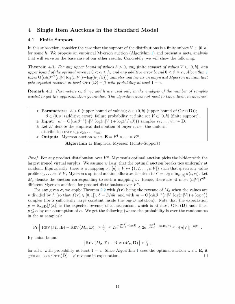
In this subsection, consider the case that the support of the distributions is a finite subset V ⊂ [0, h]for some h. We propose an empirical Myerson auction (Algorithm 1) and present a meta analysisthat will serve as the base case of our other results. Concretely, we will show the following:

Theorem 4.1. For any upper bound of values h > 0, any finite support of values V ⊂ [0, h], anyupper bound of the optimal revenue 0 < α ≤ h, and any additive error bound 0 < β ≤ α, Algorithm 1takes Θ

(αhβ−2

(n|V | log(n|V |)+log(hγ/β)

))samples and learns an empirical Myerson auction that

gets expected revenue at least Opt (D)− β with probability at least 1− γ.

Remark 4.1. Parameters α, β, γ, and h are used only in the analysis of the number of samplesneeded to get the approximation guarantee. The algorithm does not need to know them in advance.

1: Parameters: h > 0 (upper bound of values); α ∈ (0, h] (upper bound of Opt (D));β ∈ (0, α] (additive error); failure probability γ; finite set V ⊂ [0, h] (finite support).

2: Input: m = Θ(αhβ−2

(n|V | log(n|V |) + log(h/γβ)

))samples v1, . . . ,vm ∼ D.

3: Let Ei denote the empirical distribution of buyer i, i.e., the uniformdistribution over v1i, v2i, . . . , vmi.

4: Output: Myerson auction w.r.t. E = E1 × · · · × En.

Algorithm 1: Empirical Myerson (Finite-Support)

Proof. For any product distribution over V n, Myerson’s optimal auction picks the bidder with thelargest ironed virtual surplus. We assume w.l.o.g. that the optimal auction breaks ties uniformly atrandom. Equivalently, there is a mapping σ : [n]× V 7→ 1, 2, . . . , n|V | such that given any valueprofile v1, . . . , vn ∈ V , Myerson’s optimal auction allocates the item to i∗ = arg mini∈[n] σ(i, vi). Let

Mσ denote the auction corresponding to such a mapping σ. Hence, there are at most (n|V |)n|V |different Myerson auctions for product distributions over V n.

For any given σ, we apply Theorem 2.2 with f(v) being the revenue of Mσ when the values arev divided by h (so that f(v) ∈ [0, 1]), δ = β/4h, and with m = Θ

(αhβ−2

(n|V | log(n|V |) + log γ

))samples (for a sufficiently large constant inside the big-Θ notation). Note that the expectationp = Ex∈D[f(x)] is the expected revenue of a mechanism, which is at most Opt (D) and, thus,p ≤ α by our assumption of α. We get the following (where the probability is over the randomnessin the m samples):

Pr[∣∣Rev (Mσ,E)−Rev (Mσ,D)

∣∣ ≥ β2

]≤ 2e

− 2mδ2

4p+δ−ln(δ) ≤ 2e−

mβ2

40αh+ln(4h/β) ≤ γ(n|V |)−n|V | .

By union bound ∣∣Rev (Mσ,E)−Rev (Mσ,D)∣∣ < β

2 ,

for all σ with probability at least 1 − γ. Since Algorithm 1 uses the optimal auction w.r.t. E, itgets at least Opt

(D)− β revenue in expectation.

11

4.2 Bounded Support: Additive Bound

In this subsection, consider the case that the distributions have support [0, h] for some h. We seekto learn a mechanism that is optimal up to an ε additive loss in term of revenue. We show thefollowing theorem.

Theorem 4.2. Suppose the product distribution D has bounded support [0, h]. Then, for any ε > 0,there is an algorithm that takes O(h3nε−3) samples and learns a mechanism with revenue at leastOpt (D)−O(ε).

We will prove the theorem by reducing it to the finite support case. To do so, we first introducea technical lemma showing that a standard discretization of the value space decreases the optimalrevenue by at most ε additively.

Lemma 4.3 (Additive Discretization of Value Space). Given any product value distribution D′,and D′′ obtained by rounding the values from D′ to the closest multiple of ε from below, we haveOpt (D′′) ≥ Opt (D′)− ε.Proof. We follow the same strategy as in Proposition 3.1. We will prove the lemma by constructinga mechanism that gets expected revenue at least Opt (D′) − ε on D′′. Let M ′ be the optimalmechanism w.r.t. D′. Consider a mechanism M ′′ with an allocation rule that proceeds as follows:

1. Given a reported value profile v′′, let q′′i ’s be the quantiles of v′′i ’s w.r.t. D′′ (in case of apoint mass at v′′i , sample the quantile from the corresponding interval like in the proof ofProposition 3.1).

2. Let v′i’s be the values that correspond to q′′i ’s w.r.t. D′.

3. Use the allocation of mechanism M ′ for values v′i’s.

Clearly, the above allocation rule is monotone. Thus, there is a payment rule that makes it truth-ful. Further, the payment of the winner equals the threshold value above which he has non-zeroprobability to be the winner.

Next, we analyze the expected revenue of M ′′. As in Proposition 3.1, we couple all the ran-domness by first sampling the quantiles. Given any quantiles q ∈ [0, 1]n, let v′ and v′′ be thecorresponding values w.r.t. D′ and D′′ respectively. Then, by our construction of M ′′, the alloca-tion of M ′ for v′ is the same as the allocation of M ′′ for v′′, i.e., the winner is the same bidder inboth cases.

Further, the payment of each mechanism is equal to the threshold value of each winner abovewhich he remains a winner. Again, by our construction of M ′′, the quantiles of the threshold valuesin both cases are the same.

Recall that D′′ is obtained by rounding the values from D′ to the closest multiple of ε frombelow. So for any given quantile (in particular, the above threshold quantiles), the correspondingvalues in D′ and D′′ differs additively by at most ε.

Putting together, we get that the revenue of M ′ for v′, and that of M ′′ for v′′ differs additivelyby at most ε. Since this holds for all quantiles q, the lemma follows by taking expectation over therandomness of q ∈ [0, 1]n.

By rounding the values to their closest multiples of ε from below, we reduce the problem to thefinite support case with support V = 0, ε, 2ε, . . . , h, which has size h/ε. As a result, we get thefollowing Algorithm 2.

Proof of Theorem 4.2. By Theorem 4.1 and Lemma 4.3, we get that Algorithm 2 learns an empiricalMyerson auction gets revenue at least Opt (D)−O(ε) in expectation.

12

1: Parameters: h > 0 (upper bound of values); ε ∈ (0, h] (additive revenue loss);γ > 0 (failure probability).

2: Input: m = Θ(h2ε−2(nhε−1 log(nh/ε) + log γ−1)

)samples v1, . . . ,vm ∼ D.

3: Run Algorithm 1 with V = 0, ε, 2ε, . . . , h, samples rounded to the closest multiple of ε,α = h, and β = ε (h and γ remain what they are).

4: Output: The empirical Myerson auction outputted by Algorithm 1, treating any valueas the closest multiple of ε from below.

Algorithm 2: Empirical Myerson (Additive Bound for Bounded-Support Distributions)

4.3 Bounded Support: Multiplicative Bound

In this subsection, consider the case that the distributions have support [1, h] for some h. We seekto learn a mechanism that is optimal up to a 1 − ε multiplicative factor in term of revenue. Weshow the following theorem.

Theorem 4.4. Suppose the product distribution D has bounded support [1, h]. Then, for any0 < ε < 1, there is an algorithm that takes O(hnε−3) samples and learns a mechanism with revenueat least

(1−O(ε)

)Opt (D).

Similar to the case of additive approximation in the previous section, we will prove the theoremby reducing it to the finite support case. Again, we first introduce a technical lemma showingthat a standard discretization of the value space decreases the optimal revenue by at most a 1− εmultiplicative factor.

Lemma 4.5. Given any product value distribution D′, and D′′ obtained by rounding the valuesfrom D′ down to the closest power of 1− ε, we have Opt (D′′) ≥ (1− ε)Opt (D′).

Proof. The lemma follows as a simple corollary of the monotonicity of the optimal revenue (Propo-sition 3.1). Consider a distribution D′′′ that rounds the values from D′ up to the closest power of1 − ε. The difference between D′′′ and D′′ is that the former is rounded up whereas the latter isrounded down. Thus, effectively D′′′ is just D′′ scaled up by a factor of (1 − ε)−1. Clearly, theoptimal revenue of D′′ is 1− ε times that of D′′′, which by Proposition 3.1 is greater than or equalto the optimal revenue of D′.

By rounding the values to their closest powers of 1 − ε from below, we reduce the problem tothe finite support case with support V = 1, (1− ε)−1, (1− ε)−2, . . . , h, which has size h/ε. As aresult, we get the following Algorithm 3.

1: Parameters: h > 0 (upper bound of values); ε ∈ (0, 1) (multiplicative loss);γ > 0 (failure probability).

2: Input: m = Θ(hε−2(nε−1 log h log(n log h/ε) + log γ−1)

)samples v1, . . . ,vm ∼ D.

3: Run Algorithm 1 with V = 1, (1− ε)−1, (1− ε)−2, . . . , h, samples rounded to the closestpowers of 1− ε, α = Opt (D), and β = εOpt (D) (h and γ remain what they are).

4: Output: The empirical Myerson auction outputted by Algorithm 1, treating any valueas the closest power of 1− ε from below.

Algorithm 3: Empirical Myerson (Multiplicative Bound for Bounded-Support Distributions)

13

Proof of Theorem 4.4. By Lemma 4.5 and Theorem 4.1 (noting that αhβ−2 = hε−2Opt (D)−1 ≤hε−2 since Opt (D) ≥ 1), we get that Algorithm 3 learns an empirical Myerson auction gets revenueat least

(1−O(ε)

)Opt (D) in expectation.

4.4 Regular

In this subsection, we show an O(nε4

)upper bound on the sample complexity when the distributions

are regular. The challenge of this case is that the support of the distribution could be unbounded.The main technical ingredient that overcomes this challenge is to show that we can truncate thevalues down to a high enough finite quantity without losing too much revenue. This is captured inthe following lemma, whose proof is deferred to Section 4.4.1.

Lemma 4.6. Suppose 14 ≥ ε > 0 is a constant. Suppose v ≥ 1

εOpt (D). Let D1, . . . , Dn be thedistributions obtained by truncating D1, . . . , Dn at v, i.e., a sample vi from Di is obtained by firstsampling vi from Di and then letting vi = minvi, v. Then, we have

Opt(ΠiD

i)≥ (1− 4ε)Opt (D)

Suppose that Opt (D) is known, say, up to a constant factor. Then, Lemma 4.6 implies that itsuffices to consider prices between εOpt (D) and 1

εOpt (D). Further, by the standard multiplicativediscretization in Lemma 4.5, it suffices to consider prices that are powers of 1−ε. Putting together,we can restrict ourselves to ε−1 log(1

ε ) discretized values. Hence, we can apply Theorem 4.1 withα = Opt (D), β = εOpt (D), h = 1

εOpt (D), and |V | = ε−1 log(1ε ) to get the desired bound.

In order to instantiate the above approach, we design an algorithm that estimates the optimalrevenue up to a constant factor. To do this, we employ a bootstrapping approach. We consider twofamilies of simple mechanisms, namely, selling to each buyer separately, and the VCG mechanismwith duplicates.8 These simple mechanisms require relatively few samples to implement and geta good enough approximation of the optimal revenue of the original problem (e.g., [11]). We runthese simpler mechanisms with Θ(nε−1 log n

ε ) samples to find a constant approximation of optimalrevenue using Algorithm 4, whose role is summarized in Lemma 4.7.

Lemma 4.7. With probability 1−O(ε), we have 18Opt (D) ≤ Apx ≤ 8Opt (D) .

We’ll first prove the following straightforward Lemma:

Lemma 4.8. With probability 1−O(ε), we have

Opt (D) ≤ SRev ≤ 2nOpt (D)

Proof. By that maxi∈[n] Opt(Di)≤ Opt (D) ≤

∑ni=1 Opt

(Di)

and that SRevi is a 2 approxi-mation of Opt

(Di), the lemma follows.

Proof of Lemma 4.7. By Lemma 4.6 and Lemma 4.8, the optimal revenue when the values aretruncated at 1

εSRev ≥ 1εOpt (D), denoted as Opt, is at least

(1− O(ε)

)Opt (D). On one hand,

the truncated distributions are also regular. So the expected revenue of running VCG with duplicatew.r.t. the truncated values, denoted as VCG, is a 2-approximation of the optimal revenue of thetruncated distributions (Theorem 4.4 of [11]), i.e., VCG ≥ 1

2Opt. On the other hand, we haveVCG ≤ 2Opt since we are running a mechanism with two copies of each buyer. Further, therevenue from each run of the VCG with duplicate is at most 1

εSRev ≤ 2nε Opt (D) because the

8Another potential approach is to use VCG with monopoly reserves, which also gives similar guarantees.

14

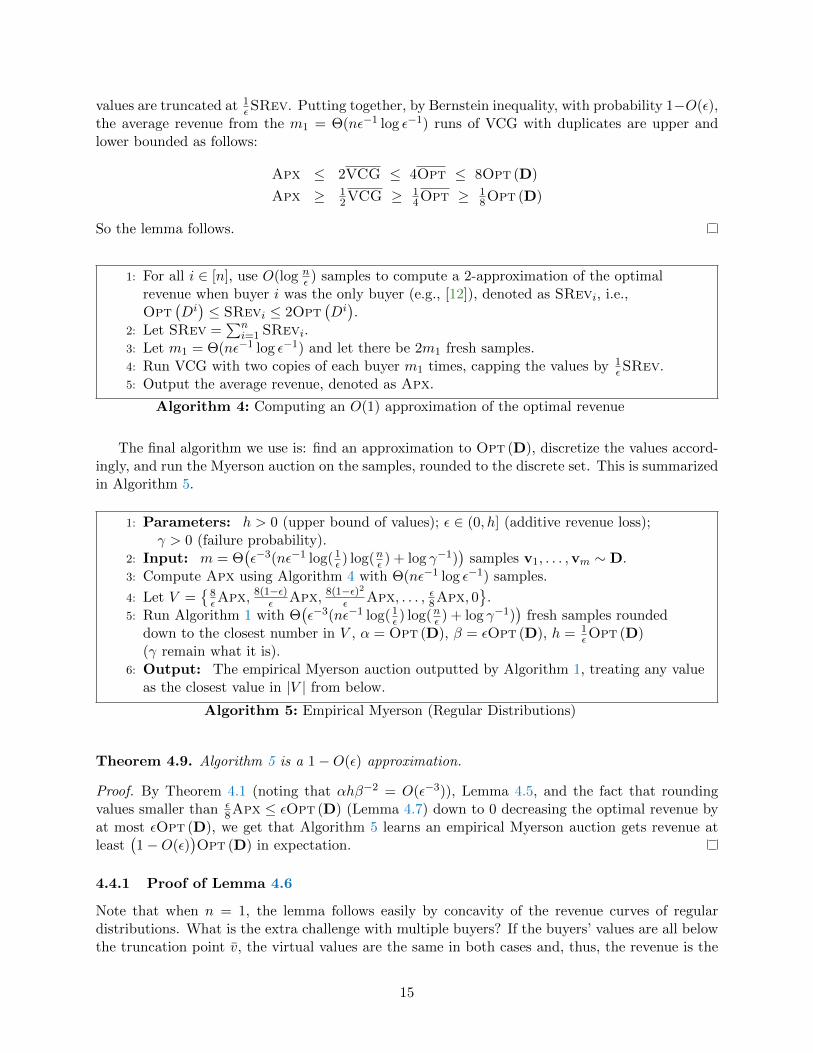
values are truncated at 1εSRev. Putting together, by Bernstein inequality, with probability 1−O(ε),

the average revenue from the m1 = Θ(nε−1 log ε−1) runs of VCG with duplicates are upper andlower bounded as follows:

Apx ≤ 2VCG ≤ 4Opt ≤ 8Opt (D)

Apx ≥ 12VCG ≥ 1

4Opt ≥ 18Opt (D)

So the lemma follows.

1: For all i ∈ [n], use O(log nε ) samples to compute a 2-approximation of the optimal

revenue when buyer i was the only buyer (e.g., [12]), denoted as SRevi, i.e.,Opt

(Di)≤ SRevi ≤ 2Opt

(Di).

2: Let SRev =∑n

i=1 SRevi.3: Let m1 = Θ(nε−1 log ε−1) and let there be 2m1 fresh samples.4: Run VCG with two copies of each buyer m1 times, capping the values by 1

εSRev.5: Output the average revenue, denoted as Apx.

Algorithm 4: Computing an O(1) approximation of the optimal revenue

The final algorithm we use is: find an approximation to Opt (D), discretize the values accord-ingly, and run the Myerson auction on the samples, rounded to the discrete set. This is summarizedin Algorithm 5.


2: Input: m = Θ(ε−3(nε−1 log(1

ε ) log(nε ) + log γ−1))

samples v1, . . . ,vm ∼ D.3: Compute Apx using Algorithm 4 with Θ(nε−1 log ε−1) samples.

4: Let V =

8εApx, 8(1−ε)

ε Apx, 8(1−ε)2ε Apx, . . . , ε8Apx, 0

.

5: Run Algorithm 1 with Θ(ε−3(nε−1 log(1


fresh samples roundeddown to the closest number in V , α = Opt (D), β = εOpt (D), h = 1

εOpt (D)(γ remain what it is).

6: Output: The empirical Myerson auction outputted by Algorithm 1, treating any valueas the closest value in |V | from below.

Algorithm 5: Empirical Myerson (Regular Distributions)

Theorem 4.9. Algorithm 5 is a 1−O(ε) approximation.

Proof. By Theorem 4.1 (noting that αhβ−2 = O(ε−3)), Lemma 4.5, and the fact that roundingvalues smaller than ε

8Apx ≤ εOpt (D) (Lemma 4.7) down to 0 decreasing the optimal revenue byat most εOpt (D), we get that Algorithm 5 learns an empirical Myerson auction gets revenue atleast

(1−O(ε)


4.4.1 Proof of Lemma 4.6

Note that when n = 1, the lemma follows easily by concavity of the revenue curves of regulardistributions. What is the extra challenge with multiple buyers? If the buyers’ values are all belowthe truncation point v, the virtual values are the same in both cases and, thus, the revenue is the

15

same. If exactly one of the buyers’ value is larger than v, the analysis is similar to the n = 1 case.It remains to bound the revenue when more than one buyers’ values are larger than v, in which casethe competition among the buyers may give an extra edge to the untruncated case. It turns outthat truncations are so rare such that the revenue from the third case of the untruncated settingcan be charged to the revenue from the second case of the truncated setting.

Truncations are Rare. Let qi = 1−F (v) denote the quantile of value v w.r.t. Di. Let φi(qi) andφi(qi) denote the virtual value at quantile qi w.r.t. Di and Di respectively. Then, φi(qi) = φi(qi) ifqi < qi ≤ 1 and v otherwise. It is easy to see that for any i ∈ [n], we have qi ≤ ε. We also show thefollowing more refined bound on qis.

Lemma 4.10. The probability that at least one buyer has value greater than or equal to v is atmost ε and is at least (1− ε)

∑i∈[n] qi, i.e.,

ε ≥ 1−∏i∈[n](1− qi) ≥ (1− ε)

∑i∈[n] qi

Charging Argument. Note that both Di and Di are regular, so Myerson’s auction simply picksthe buyer with the maximum virtual surplus, and the revenue is the virtual welfare thus obtained.Given a quantile vector q, let H(q) = i ∈ [n] : qi ≤ qi denote the buyers whose values are higherthan v; let L(q) = [n] \H(q) denote the set of buyers whose values are smaller than v. We boundthe ratio separately, for the high value buyers and the low value buyers, as below.∫

[0,1]n\∏j [qj ,1] maxi φi(qi)d

nq ≥ (1− 2ε)∫

[0,1]n maxi∈H(q) φi(qi)dnq, and (2)∫∏

j [qj ,1] maxi φi(qi)dnq ≥ (1− 2ε)

∫[0,1]n maxi∈L(q) φi(qi)d

nq. (3)

Before we prove Equations 2 and 3 we need the following Lemma:

Lemma 4.11. For any i ∈ [n], we have qi ≤ ε.

Proof. Note that serving buyer i as if he was the only buyer with a reserve price v give revenue qiv,which must be less than or equal to the optimal revenue Opt (D). The lemma then follows fromthat v ≥ 1

εOpt (D).

Proof of (2): Note that for any i and any qi < qi, φi(qi) = v. Thus, the LHS of (2) is lowerbounded by ∫

[0,1]n\∏i[qi,1]

vdnq =(1−

∏i∈[n]

(1− qi))v ≥ (1− ε)

∑i∈[n]

qiv

where the inequality follows by Lemma 4.10. On the other hand, the RHS (omitting the 1 − 2εfactor) is upper bounded by∫

[0,1]nmaxi∈H(q)

φi(qi)dnq ≤

∫[0,1]n

∑i∈H(q)

maxφi(qi), 0

dnq

≤∑i∈[n]

∫[0,qi]

maxφi(qi), 0dqi

Therefore, to show (2), it suffices to show that for every i ∈ [n],

qiv ≥ (1− ε)∫qi∈[0,qi]

maxφi(qi), 0

16

Let Ri(q) denote the revenue of a single-buyer auction with a reserve price that has quantile q w.r.t.Di. The LHS of the above is the revenue of a single-buyer auction with reserve price v w.r.t. Di,i.e., Ri(qi). The RHS is the maximum revenue of a single-buyer auction with a reserve price atleast v, i.e., maxq∈[0,qi]Ri(q). Note that Di’s being regular implies that Ri(q) is a concave functionover [0, 1] and Ri(1) ≥ 0. Thus, we have that Ri(qi) ≥ (1 − qi) maxq∈[0,qi]Ri(q). The inequalitythen follows by qi ≤ ε (Lemma 4.11).

Proof of (3): Note that for any q ∈∏j∈[n][qj , 1], we have L(q) = [n]. So we can rewrite the LHS

of (3) as follows. ∫∏j [qj ,1]

maxi∈[n]

φi(qi)dnq =

∫∏j [qj ,1]

maxi∈L(q)

φi(qi)dnq

For any q−i ∈ [0, 1]n−1, any qi < qi ≤ q′i, consider q = (qi,q−i) and q′ = (q′i,q−i). We have thatL(q) ⊂ L(q′), and for any i ∈ L(q), qi = q′i. Thus, maxi∈L(q) φi(qi) ≤ maxi∈L(q′) φi(q

′i). Therefore,

we have that∫∏j [qj ,1]

maxi∈L(q)

φi(qi)dnq ≥ (1− q1)

∫[0,1]×

∏nj=2[qj ,1]

maxi∈L(q)

φi(qi)dnq

≥ (1− q1)(1− q2)

∫[0,1]2×

∏nj=3[qj ,1]

maxi∈L(q)

φi(qi)dnq

≥ . . .

≥∏j∈[n]

(1− qj)∫

[0,1]nmaxi∈L(q)

φi(qi)dnq

Finally, by Lemma 4.10, we have that∏j∈[n](1− qj) ≥ 1− ε. Putting together proves (3).

4.5 Monotone Hazard Rate

In this subsection, we show an O(nε3

)upper bound on the sample complexity when the distributions

have monotone hazard rate. The algorithm is almost identical to that for regular distributions,except that we have a better tail bound due to the assumption of monotone hazard rate. Inparticular, we will make use of the extreme value theorem by Cai and Daskalakis [5].

Lemma 4.12 (Theorem 18 of [5]). Suppose 14 ≥ ε > 0 is a constant. Suppose v ≥ log(1

ε )Opt (D).Let D1, . . . , Dn be the distributions obtained by truncating D1, . . . , Dn at v, i.e., a sample vi fromDi is obtained by first sampling vi from Di and then letting vi = minvi, v. Then, we have

Opt(ΠiD

i)≥(1−O(ε)

)Opt (D)

Theorem 4.13. Algorithm 6 is a 1−O(ε) approximation.

Proof. By Theorem 4.1 (noting that αhβ−2 = O(ε−2 log(1ε ))), Lemma 4.5, and the fact that round-

ing values smaller than ε8Apx ≤ εOpt (D) (Lemma 4.7) down to 0 decreasing the optimal revenue

by at most εOpt (D), we get that Algorithm 5 learns an empirical Myerson auction gets revenueat least

(1−O(ε)


17


2: Input: m = Θ(ε−3(nε−1 log(1


samples v1, . . . ,vm ∼ D.3: Compute Apx using Algorithm 4 with Θ(nε−1 log ε−1) samples.4: Let V =

8 log(1

ε )Apx, 8(1− ε) log(1ε )Apx, 8(1− ε)2 log(1

ε )Apx, . . . , ε8Apx, 0

.5: Run Algorithm 1 with Θ

(ε−2 log(1

ε )(nε−1 log(1


fresh samples roundeddown to the closest number in V , α = Opt (D), β = εOpt (D), h = log(1

ε )Opt (D)(γ remain what it is).

6: Output: The empirical Myerson auction outputted by Algorithm 1, treating any valueas the closest value in |V | from below.

Algorithm 6: Empirical Myerson (MHR Distributions)

5 Signal Auctions Upper Bounds

5.1 Single Agent

In this subsection we sketch a proof of the O( log(1/ε)q(ε)ε3

)upper bound for the Signals model, for n = 1.

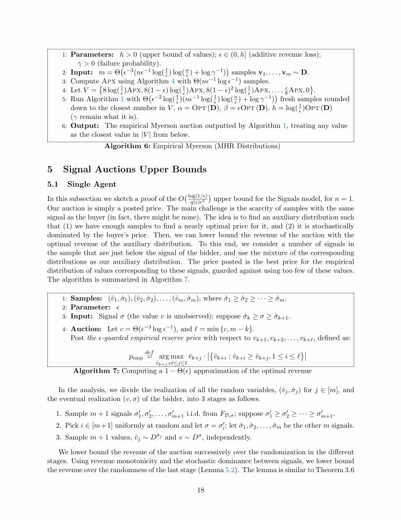
Our auction is simply a posted price. The main challenge is the scarcity of samples with the samesignal as the buyer (in fact, there might be none). The idea is to find an auxiliary distribution suchthat (1) we have enough samples to find a nearly optimal price for it, and (2) it is stochasticallydominated by the buyer’s prior. Then, we can lower bound the revenue of the auction with theoptimal revenue of the auxiliary distribution. To this end, we consider a number of signals inthe sample that are just below the signal of the bidder, and use the mixture of the correspondingdistributions as our auxiliary distribution. The price posted is the best price for the empiricaldistribution of values corresponding to these signals, guarded against using too few of these values.The algorithm is summarized in Algorithm 7.

1: Samples: (v1, σ1), (v2, σ2), . . . , (vm, σm), where σ1 ≥ σ2 ≥ · · · ≥ σm.2: Parameter: ε3: Input: Signal σ (the value v is unobserved); suppose σk ≥ σ ≥ σk+1.

4: Auction: Let c = Θ(ε−3 log ε−1), and ` = min c,m− k.Post the ε-guarded empirical reserve price with respect to vk+1, vk+2, . . . , vk+`, defined as:

pempdef= arg max

vk+j :ε`≤j≤`vk+j ·

∣∣vk+i : vk+i ≥ vk+j , 1 ≤ i ≤ `∣∣

Algorithm 7: Computing a 1−Θ(ε) approximation of the optimal revenue

In the analysis, we divide the realization of all the random variables, (vj , σj) for j ∈ [m], andthe eventual realization (v, σ) of the bidder, into 3 stages as follows.

1. Sample m+ 1 signals σ′1, σ′2, . . . , σ

′m+1 i.i.d. from FD,σ; suppose σ′1 ≥ σ′2 ≥ · · · ≥ σ′m+1.

2. Pick i ∈ [m+1] uniformly at random and let σ = σ′i; let σ1, σ2, . . . , σm be the other m signals.

3. Sample m+ 1 values, vj ∼ Dσj and v ∼ Dσ , independently.

We lower bound the revenue of the auction successively over the randomization in the differentstages. Using revenue monotonicity and the stochastic dominance between signals, we lower boundthe revenue over the randomness of the last stage (Lemma 5.2). The lemma is similar to Theorem 3.6

18

of [12] with the extra complication that the sample values are not iid from the auxiliary distribution.Next, we lower bound the revenue over the randomness of the last two stages (Lemma 5.3), andfinally over the randomness of all three stages (Lemma 5.4). The revenue guarantee then followsfrom Definition 1.

Let Rev (p,D) denote the expected revenue of posting price p when the underlying distributionis D.

Definition 2 (Truncated distributions). Given any distribution D over [0,+∞) and any 0 < δ < 1,let Dtrunc

δ denote the distribution obtained by replacing the entire top δ of the probability mass ofD with a point mass. Formally, if F is the c.d.f. of D then the c.d.f. of Dtrunc

δ is identical to F forall values less than F−1(1− δ), and the c.d.f of Dtrunc

δ at F−1(1− δ) is 1.

Let D denote the mixed distribution of Dσk+1 , Dσk+2 , . . . , Dσk+` . That is, if we want to drawa value from D, we first sample i from 1, 2, . . . , ` uniformly at random, and then draw a valuefrom Dσk+i . It is easy to verify the following claims:

Claim 5.1. Dσ Dtruncε Dσk+` trunc

ε .

Claim 5.2. If D D′, then for any price p ≥ 0 we have Rev (p,D) ≥ Rev (p,D′).

Claim 5.3. Opt (Dtruncε ) ≥ (1− ε)Opt (D), for all regular distributions D.

We first need to show that:

Lemma 5.1.

E[Rev

(pemp, D

truncε

)|σ1, . . . , σm, σ

]≥ (1− ε)2Opt

(Dtruncε

),

where the expectation is over the random draws of values from the Dσi’s.

Proof. For the purposes of this proof we’ll relax notation and not write the conditioning on

σ1, . . . , σm, σ. Let p∗ be the optimal price for Dtruncε , i.e. Rev

(p∗, Dtrunc

ε

)= Opt

(Dtruncε

). Also

let Etruncε be the uniform distribution over V = vk+j : ε` ≤ j ≤ `, where vk+j is drawn from

Dσk+j . Using standard Chernoff bounds it’s easy to see that w.h.p.:

Rev(p∗, Etrunc

ε

)≥ (1− ε)Rev

(p∗, Dtrunc

ε

), (4)

i.e. expected revenue of p∗ in Etruncε is a good estimate of it’s revenue in Dtrunc

ε . Using a similarproof (plus union bound) we can show that the same is true for all vk+z ∈ V , and thus:

Rev(pemp, D

truncε

)≥ (1− ε)Rev

(pemp, E

truncε

), (5)

Finally, we’ll show that the value in V with the highest revenue in Etruncε , i.e. pemp, has revenue in

Etruncε at least the revenue of p∗ in Etrunc

ε :

Rev(pemp, E

truncε

)≥ Rev

(p∗, Etrunc

ε

)(6)

19

Etruncε is uniform over discrete values; the optimal (in terms of revenue) posted price chosen out

of those values is also optimal overall. Putting it all together we get that w.h.p.:

Rev(pemp, D

truncε

)≥ (1− ε)Rev

(pemp, E

truncε

)Equation: 5

≥ (1− ε)Rev(p∗, Etrunc

ε

)Equation: 6

≥ (1− ε)2Rev(p∗, Dtrunc

ε

)Equation: 4

= (1− ε)2Opt(Dtruncε

)

The main lemma for this stage is the following:

Lemma 5.2.E[Rev (pemp, D

σ) |σ1, . . . , σm, σ]≥ (1− ε)3Opt

(Dσk+`

).

Proof.

E[Rev (pemp, D

σ) |σ1, . . . , σm, σ]≥ E

[Rev

(pemp, D

truncε

)|σ1, . . . , σm, σ

](Claims 5.2 and 5.1)

≥ (1− ε)2Opt(Dtruncε

)(Lemma 5.1)

≥ (1− ε)2Opt(Dσk+` trunc

ε

)(Theorem 2.1 and Claim 5.1)

≥ (1− ε)3Opt(Dσk+`

)(Claim 5.3)

Next, we lower bound the revenue of the above auction over the randomness of the last twostages:

Lemma 5.3.

E[Rev (pemp, D

σ) |σ′1, . . . , σ′m+1

]≥ (1− ε)3

m+ 1

m+1∑i=`+1

Opt(Dσ′i

)Proof. Note that

E[Rev (pemp, D

σ) |σ′1, . . . , σ′m+1

]=

1

m+ 1

m+1∑i=1

E[Rev (pemp, D

σ) |σ′1, . . . , σ′m+1, σ = σi]

For any i ≤ m+ 1− `, by Lemma 5.2, we get that

E[Rev (pemp, D

σ) |σ′1, . . . , σ′m+1, σ = σi]≥ (1− ε)3Opt

(Dσ′i+`

)Therefore, we have

E[Rev (pemp, D

σ) |σ′1, . . . , σ′m+1

]≥ (1− ε)3

m+ 1

m+1−`∑i=1

Opt(Dσ′i+`

)=

(1− ε)3

m+ 1

m+1∑i=`+1

Opt(Dσ′i

)

20

Finally, we will lower bound the revenue of the above auction over the randomness of all threestages.

Lemma 5.4.

E[Rev (pemp, D

σ)]≥ (1− ε)3

∫ F−1D,σ(1− c

m+1)

0Opt (Dσ) dFD,σ

Proof. Recall that σ′1, . . . , σ′m+1 are i.i.d. from FD,σ. Thus, we have

1

m+ 1

m+1∑i=1

Opt(Dσ′i

)=

∫ 1

0Opt (Dσ) dFD,σ

Let us compare the LHS of the above with the RHS of (5.3) (removing the (1 − ε)3 factor), i.e.,1

m+1

∑m+1i=`+1 Opt

(Dσ′i

). The latter drops ` of the m + 1 signals in the summation and, thus,

effectively drops `m+1 of the probability mass in the expectation. Recall that Dσ stochastically

dominates Dσ′ for any σ ≥ σ′. So the worst-case scenario is dropping the contributions fromsignals σ ∈ [1− c

m+1 , 1]. The lemma then follows.

5.2 Multiple agents

In this subsection, we show how to solve the multi-agent problem in the Signals model, buildingon techniques in the single-agent problem and in the non-iid model of the multi-agent problem.Formally, we prove the following sample complexity upper bound.

Theorem 5.5 (Upper bound for multiple agents). There exists a mechanism for selling to n agentsin the Signals model, that has a sample complexity, against regular distributions which have a q-bounded tail in the signal space, of

O

(n2

q(ε)ε4log2 n

ε

)High-level ideas. We combine the ideas from the single-agent signal case (Section 5.1) and the

multi-agent no-signal case (Section 4). For each agent, consider ` = Θ(n2

ε4log n

ε ) sample signals thatare closest to the agent’s signal from below, and using the corresponding ` sample values in placeof the actual samples from his true distribution, we run the the empirical Myerson’s auction withpreconditioning in Section 4. Like in the single agent case, we would like to show that the expectedrevenue of the auction is almost as good as the optimal revenue when each agent’s distribution isreplaced by the distribution whose signal is the `-th closest to the agent’s signal from below. Then,we can use the small tail assumption in the signal space to show that the auction gives nearlyoptimal revenue.

There are two caveats, one in the algorithm and one in the analysis. First, the implementationof the empirical Myerson’s auction in Section 4 uses the VCG mechanism with duplicate agentsto estimate the optimal revenue up to a constant factor, exploiting regularity of the distributions.The algorithm in the Signals model, however, needs to estimate the optimal revenue when eachagent’s distribution is replaced by the mixture of the ` distributions whose signals are closest to theagent’s signal from below. The mixture of regular distributions is not necessarily regular. Thus,we turn to a coarser n-approximation.

Further, the analysis for the single-agent case uses a strong notion of revenue monotonicity,which holds regardless of the mechanism being used.9 With multiple agents, we need to make do

9This is true in the single agent case since these mechanisms are posted price mechanisms.

21

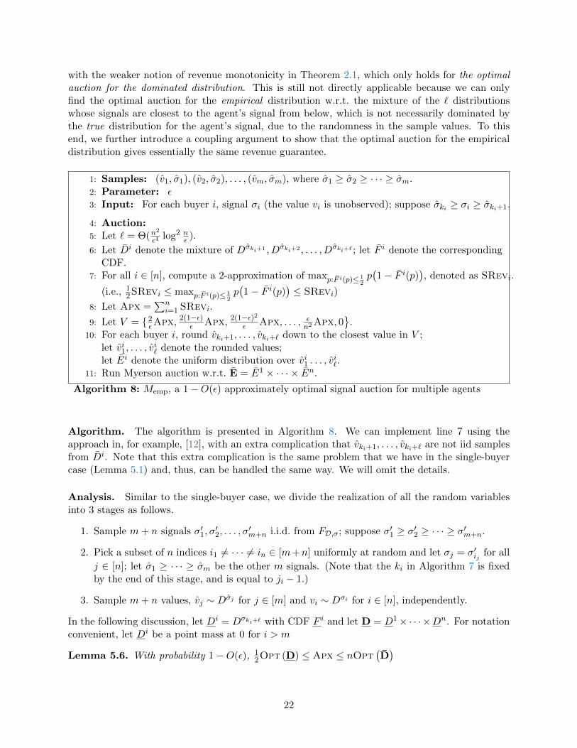
with the weaker notion of revenue monotonicity in Theorem 2.1, which only holds for the optimalauction for the dominated distribution. This is still not directly applicable because we can onlyfind the optimal auction for the empirical distribution w.r.t. the mixture of the ` distributionswhose signals are closest to the agent’s signal from below, which is not necessarily dominated bythe true distribution for the agent’s signal, due to the randomness in the sample values. To thisend, we further introduce a coupling argument to show that the optimal auction for the empiricaldistribution gives essentially the same revenue guarantee.

1: Samples: (v1, σ1), (v2, σ2), . . . , (vm, σm), where σ1 ≥ σ2 ≥ · · · ≥ σm.2: Parameter: ε3: Input: For each buyer i, signal σi (the value vi is unobserved); suppose σki ≥ σi ≥ σki+1.

4: Auction:5: Let ` = Θ(n

2

ε4log2 n

ε ).

6: Let Di denote the mixture of Dσki+1 , Dσki+2 , . . . , Dσki+` ; let F i denote the correspondingCDF.

7: For all i ∈ [n], compute a 2-approximation of maxp:F i(p)≤ 12p(1− F i(p)

), denoted as SRevi.

(i.e., 12SRevi ≤ maxp:F i(p)≤ 1

2p(1− F i(p)

)≤ SRevi)

8: Let Apx =∑n

i=1 SRevi.

9: Let V = 2εApx, 2(1−ε)

ε Apx, 2(1−ε)2ε Apx, . . . , ε

n2Apx, 0

.10: For each buyer i, round vki+1, . . . , vki+` down to the closest value in V ;

let vi1, . . . , vi` denote the rounded values;

let Ei denote the uniform distribution over vi1 . . . , vi`.

11: Run Myerson auction w.r.t. E = E1 × · · · × En.

Algorithm 8: Memp, a 1−O(ε) approximately optimal signal auction for multiple agents

Algorithm. The algorithm is presented in Algorithm 8. We can implement line 7 using theapproach in, for example, [12], with an extra complication that vki+1, . . . , vki+` are not iid samplesfrom Di. Note that this extra complication is the same problem that we have in the single-buyercase (Lemma 5.1) and, thus, can be handled the same way. We will omit the details.

Analysis. Similar to the single-buyer case, we divide the realization of all the random variablesinto 3 stages as follows.

1. Sample m+ n signals σ′1, σ′2, . . . , σ

′m+n i.i.d. from FD,σ; suppose σ′1 ≥ σ′2 ≥ · · · ≥ σ′m+n.

2. Pick a subset of n indices i1 6= · · · 6= in ∈ [m+n] uniformly at random and let σj = σ′ij for all

j ∈ [n]; let σ1 ≥ · · · ≥ σm be the other m signals. (Note that the ki in Algorithm 7 is fixedby the end of this stage, and is equal to ji − 1.)

3. Sample m+ n values, vj ∼ Dσj for j ∈ [m] and vi ∼ Dσi for i ∈ [n], independently.

In the following discussion, let Di = Dσki+` with CDF F i and let D = D1× · · ·×Dn. For notationconvenient, let Di be a point mass at 0 for i > m

Lemma 5.6. With probability 1−O(ε), 12Opt (D) ≤ Apx ≤ nOpt

(D)

22

Proof. The first inequality holds because

SRevi ≥ maxp:F i(p)≤ 1

2

p(1− F i(p)

)(definition of SRevi)

≥ maxp:F i(p)≤ 1

2

p(1− F i(p)

)(F i F i)

≥ 1

2maxp≥0

p(1− F i(p)

)(regularity of Di)

and∑

i∈[n] maxp≥0 p(1 − F i(p)

)=∑

i∈[n] Opt(Di)≥ Opt (D). The second inequality holds

because SRevi ≤ Opt(D).


Opt(D)≥(1−O(ε)

)Opt (D)−O(ε)Opt (D) .

Proof. By Lemma 5.6 and Lemma 4.6, truncating D at 2εApx ≥ 1

εOpt (D) decreases the optimalrevenue by at most at 1 − O(ε) factor. Further, by Lemma 4.5, rounding values to the closestpower of 1− ε decreases the optimal revenue by at most another 1 − ε factor. Finally, by Lemma5.6 rounding all values less than ε

n2Apx ≤ εnOpt

(D)

to 0 decreases the revenue by at mostεOpt

(D).

As a simple corollary of the above lemma and Theorem 2.2, 10 we have the following lemma.


Opt(E)≥(1−O(ε)


Next, we prove the key lemma that lower bounds the expected revenue of the empirical Myersonauction w.r.t. E if we run it on D, conditioned on the realization of signals.

Lemma 5.9. With probability 1−O(ε) (over randomness of the sample values), we have

E[Rev (Memp,D) |σ1, . . . , σm, σ1, . . . , σn

]≥(1−O(ε)


Proof. Let us first explain the proof structure. If D stochastically dominates E, then the lemmafollows by Lemma 5.8 and revenue monotonicity (Theorem 2.1). However, despite the fact that Dstochastically dominates D, it does not necessarily dominates E due to randomness in the samplevalues. To get around this obstacle, we designed for each buyer i a set of random values coupledwith the sample values vki+j , 1 ≤ j ≤ `, and the uniform distribution over them Ei such that (1) Estochastically dominate E, and (2) the revenue of any optimal mechanism w.r.t. some distributionover the set of discretized values when we run it on E is a 1 − O(ε) approximation of its revenueon D. Then, we can show that the revenue of the empirical Myerson auction (w.r.t. E) on D is atleast a 1−O(ε) fraction of its revenue on E, which is greater than or equal to its revenue on E.

Concretely, for every 1 ≤ j ≤ `, let qj =(1 − F σki+j (vki+j)

)be the quantile of vki+j w.r.t.

Dσki+j ; let vj be the value with quantile qj w.r.t. Di. Note that qj is uniform from [0, 1] overrandom realization of vki+j conditioned on σki+j . So vj , 1 ≤ j ≤ `, are i.i.d. samples from Di. LetEi be the uniform distribution over vj , 1 ≤ j ≤ `.

10Again, there is an extra complication that the sample values are not iid from the mixture distributions, whichcan be handled using the approach in Lemma 5.1.

23

By our construction and that Di stochastically dominates Dσki+j for any 1 ≤ j ≤ `, weget that E stochastically dominates E. Further, by revenue monotonicity (Theorem 2.1), wehave Rev (Memp,E) ≥ Rev

(Memp, E

). Recall that we can alter E such that the optimal auc-

tion is unique (Remark 2.1). Thus, by Theorem 2.2, we have that Rev (Memp,D) ≥(1 −

O(ε))Rev (Memp,E). Putting together with Lemma 5.8 proves the lemma.

As a simple corollary, we have the following lemma.


E[Rev (Memp,D)

]≥(1−O(ε)

)E[Opt (D)

]−O(ε)E

[Opt (D)

].

Finally, we relate E[Opt (D)

]with E

[Opt (D)

]by proving the following lemma.

Lemma 5.11. Over the randomness of all three stages, we have

E[Opt (D)

]≥ (1− ε)E

[Opt (D)

]Proof. Given Lemma 5.10, it suffices to relate E

[Opt (D)

]with E

[Opt (D)

]. First, we consider

the expectation over the randomness of the last two stages. Conditioned on the realization ofsignals σ′1, . . . , σ

′m+n, over the randomness of the choice of i1, . . . , in and random realization of the

corresponding values, we can write the expectation of the optimal revenue w.r.t. D as follows.

E[Opt (D) |σ′1, . . . , σ′m+n

]=

1(m+nn

) ∑i1,...,in⊂[m+n]

Opt(Dσ′i1+` × · · · ×Dσ′in+`

)=

1(m+nn

) ∑i1,...,in⊂`+1,...,`+m+n

Opt(Dσ′i1 × · · · ×Dσ′in

)≥ 1(

m+nn

) ∑i1,...,in⊂`+1,...,m+n

Opt(Dσ′i1 × · · · ×Dσ′in

)Next, we consider the expectation of over the randomness of the first stage. Note that ` ≤

q(ε)m + n. Taking expectation over random realization of σ′1, . . . , σ′m+n, the RHS of the above

inequality is lower bounded by

Eσ1,...,σn∼FD,σ [1∀i ∈ [n], FD,σ(σi) ≤ 1− q(ε)Opt (Dσ1 × · · · ×Dσn)]

By the small tail assumption in signal space (Definition 1), this is at least (1− ε)E[Opt (D)

]. So

the lemma follows.

Proof of Theorem 5.5. It follows from Lemma 5.10 and 5.11.

5.3 Lower bounds for n = 1

Theorem 5.12. The sample complexity of any single agent mechanism against any q-boundeddistribution in the Signals model is

Ω

(log (1/q(ε))

ε4

).

24

Proof. Our instance will havelog 1

α2 log(1−18ε) + 1 conditional distributions. Let N =

log 1α

2 log(1−18ε) ≈logαε .

For the i-th conditional distribution (that is the distribution conditioned on signal σi) we will havetwo candidate distributions Dσi

1 and Dσi2 , and it will be impossible to extract high revenue from

that conditional, without seeing at least 1ε3

samples (from that conditional), even when havingexact knowledge of the rest of the distributions. The expected revenue from each conditional willbe approximately the same, thus, in order for a pricing algorithm to achieve high expected revenueoverall, it will have to achieve high expected revenue in most of the conditionals.

Our construction works as follows: for each i ∈ [0, N ] let

ci =1

(1− 2ε0)2i.

Dσi1 is the distribution with c.d.f

F i1 (x) = 1− cix+ ci

and p.d.f

f i1 =ci

(x+ ci)2 .

Dσi2 has c.d.f

F i2 (x) =

1− cix+ci

if x ∈[0, (1−2ε0)ci

2ε0

]1− ci(1−2ε0)2

x−ci(1−2ε0) if x > (1−2ε0)ci2ε0

and p.d.f.

f i2 (x) =

ci

(x+ci)2 if x ∈

[0, (1−2ε0)ci

2ε0

]ci(1−2ε0)2

(x−ci(1−2ε0))2if x > (1−2ε0)ci

2ε0

where ε0 = 9ε.The revenue curves as a function of the price are

Ri1 (x) =xcix+ ci

Ri2 (x) =

xcix+ci

if x ∈[0, (1−2ε0)ci

2ε0

]xci(1−2ε0)2

x−ci(1−2ε0) if x > (1−2ε0)ci2ε0

and as a function of the quantile space

Ri1 (q) = ci (1− q)

Ri2 (q) =

ci

((1− 2ε0)2 + q (1− 2ε0)

)if q ∈ [0, 2ε0]

ci (1− q) if q ∈ [2ε0, 1]

Conditioned on seeing signal σi the Myerson revenue is ci for Dσi1 and ci (1− 2ε0) for Dσi

2 . Noticethat both Dσi

1 and Dσi2 first-order stochastically dominate both D

σi−1

1 and Dσi−1

2 (and are dominated

by the Dσi+1 ’s). Also, we have that c0 = 1 and cN = (1− 2ε0)−2N = (1− 18ε)−2 12

log1−18ε1α = α,

thus the gap between the highest and the lowest revenue is α.In order to make the expected revenue from each conditional approximately the same, we set

the probability pi of seeing signal σi equal to γ · 1ci

, where γ is the normalizing factor, i.e.

γ =1∑Nj=0

1cj

25

.The optimal expected revenue is upper bounded by:

OPT =N∑i=0

piOpt (Dσi) ≤N∑i=0

cipi = γ(N + 1)

Dropping pN in probability mass in signal space results in dropping about γ in terms of revenue,i.e. 1

N of the total revenue. Dropping pN+pN−1 results in dropping a 2N fraction of the total revenue,

and so on; thus, in order to drop an ε fraction of the total revenue, and since N is approximatelylogαε , we need to drop

∑Ni=N−logα pi in probability. This simplifies to(

(1− 2ε)

4ε(1− ε)

)2

· 1

α· 1

α2 log(1−2ε).

Using this, we can get the following relation between q(ε) and α:

logα ≈ log

(1

q(ε)

)(7)

Claim 5.4. Any pricing algorithm that is (1 − ε) approximate for this instance must be (1 − 3ε)approximate for at least half of the signals.

Proof. Assume that we have a (1 − ε) approximate algorithm, and there exists a set of signals Asuch that |A| > N+1

2 and for every signal σi ∈ A: E [R|σi] < (1− 3ε)Opt (Dσi). We will show thatthe total expected revenue R of the algorithm is less than (1− ε) of OPT .

R =N∑i=0

pi E [R|σi] =∑i∈A

pi E [R|σi] +∑i/∈A

pi E [R|σi]

<∑i∈A

(1− 3ε) piOpt (Dσi) +∑i/∈A

piOpt (Dσi) = OPT − 3ε∑i∈A

piOpt (Dσi)

< OPT − 3ε|A| (1− 2ε0) γ

Remember that γ ≥ 1N+1OPT , so 3ε|A| (1− 2ε0) γ ≥ 3

2 (1− 2ε0) εOPT > εOPT .Thus we have:

R < (1− ε)OPT

a contradiction.

We will proceed to show that in order to (1− 3ε) approximate the revenue for a given signal σi,any pricing algorithm requires Ω

(1ε3

)samples from that signal. Thus, since any (1−ε) approximate

pricing algorithm requires Ω(

1ε3

)approximate in at least N+1

2 >log 1

α4 log(1−18ε) of the signals, the total

number of signals required is Ω(

log 1α

2 log(1−18ε)1ε3

), which is Ω

(logαε4

), and thus using equation 7 we

get the desired lower bound for q-bounded distributions.

Lemma 5.13. Any pricing algorithm that is (1 − 3ε) approximate for both Dσi1 and Dσi

2 requiresΩ(

1ε3

)samples from the distribution conditioned on σi.

26

Proof. First, notice that even exact knowledge of the distributions conditioned on the rest of thesignals does not help here; we’re back to a one-distribution problem.

We will follow a similar approach to [12]: we will first bound the KL divergence of Dσi1 and

Dσi2 , then show that the (1− 9ε) = (1− ε0) optimal price sets are disjoint. We state here, without

proofs, a theorem and a lemma from [12] that we use:

Theorem 5.14 (Theorem 4.2 from [12]). If value distributions D1 and D2 have disjoint (1− 3ε′)approximate price sets, and there is a pricing algorithm that is (1 − ε′) approximate for both D1

and D2, then the algorithm uses at least 49

1DKL(D1‖D2)+DKL(D2‖D1) samples.

Lemma 5.15 (Lemma 4.4 from [12]). If distributions D1 and D2 with densities f1 and f2 satisfy

that (1 + ε′)−1 ≤ f1(ω)f2(ω) ≤ (1 + ε′) for every ω ∈ Ω, and there is a subset of outcomes Ω′ such that

p1(ω) = p2(ω) for every ω ∈ Ω′, then

DKL (D1‖D2) +DKL (D2‖D1) ≤ (ε′)2(1− p1

(Ω′))

Notice that:

f i1f i2

=

1 if x ∈[0, (1−2ε0)ci

2ε0

]ci

ci(1−2ε0)2· (x−ci(1−2ε0))2

(x+ci)2 if x > (1−2ε0)ci

2ε0

Thus it holds thatf i1f i2∈[(1− 2ε0)2 , (1− 2ε0)2

], and thus

f i1f i2∈[(

1 + ε01−2ε0

)−1,(

1 + ε01−2ε0

)].

Dσi1 and Dσi

2 are identical for x ≤ (1−2ε0)ci2ε0

. In quantile space, this corresponds to q ≥ 2ε0.Thus, by applying Lemma 5.15 we have that:

DKL (Dσi1 ‖D

σi2 ) +DKL (Dσi

2 ‖Dσi1 ) ≤

(ε0

1− 2ε0

)2

2ε0 =2ε30

(1− 2ε0)2 (8)

Moreover, the (1− ε0) price sets are disjoint, by comparing the revenue as a function of theprice:

Ri1(x) ≥ (1− ε0)ci iff x ≥ ci(1− ε0)

ε0

and

Ri2(x) ≥ (1− ε0)(1− 2ε0)ci iff x ∈[

(1− 3ε0 + 2ε20)ci3ε0 − 2ε20

,ci(1− ε0)(1− 2ε0)

ε0

]By combining equation 8 with the above observation, and Theorem 5.14 (ε′ = 3ε) we get the

desired bound.

6 Extensions

In this section, we will explain how to use the techniques developed in this paper to show samplecomplexity upper bounds for several natural extensions of the settings discussed in the main text.A summary of the results in the extended settings is presented in Table 2 and Table 3. Next, wewill present a brief introduction of these extensions. Then, in Section 6.1 and Section 6.2, we willsketch the key differences in the algorithm and the analysis of the extensions compared to those inthe main text.

27

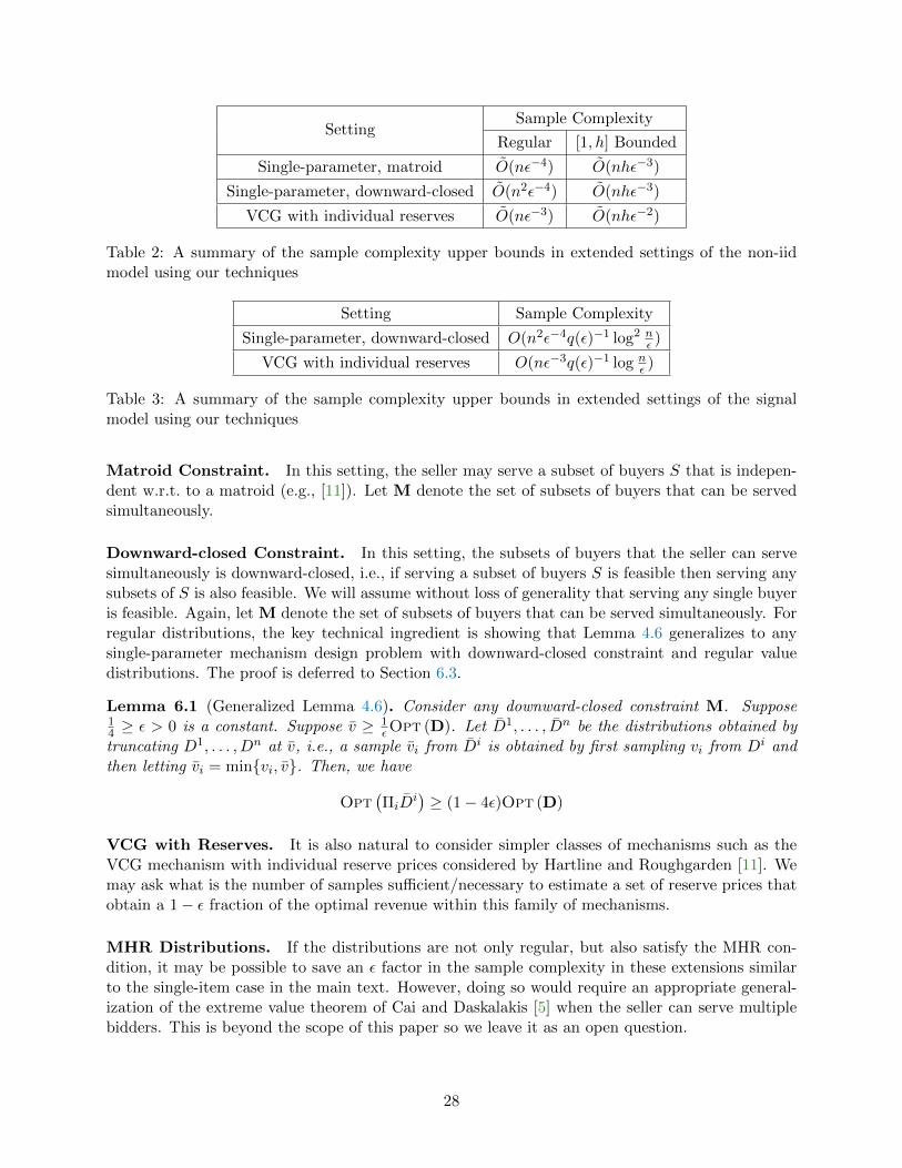
SettingSample Complexity

Regular [1, h] Bounded

Single-parameter, matroid O(nε−4) O(nhε−3)

Single-parameter, downward-closed O(n2ε−4) O(nhε−3)

VCG with individual reserves O(nε−3) O(nhε−2)

Table 2: A summary of the sample complexity upper bounds in extended settings of the non-iidmodel using our techniques

Setting Sample Complexity

Single-parameter, downward-closed O(n2ε−4q(ε)−1 log2 nε )

VCG with individual reserves O(nε−3q(ε)−1 log nε )

Table 3: A summary of the sample complexity upper bounds in extended settings of the signalmodel using our techniques

Matroid Constraint. In this setting, the seller may serve a subset of buyers S that is indepen-dent w.r.t. to a matroid (e.g., [11]). Let M denote the set of subsets of buyers that can be servedsimultaneously.

Downward-closed Constraint. In this setting, the subsets of buyers that the seller can servesimultaneously is downward-closed, i.e., if serving a subset of buyers S is feasible then serving anysubsets of S is also feasible. We will assume without loss of generality that serving any single buyeris feasible. Again, let M denote the set of subsets of buyers that can be served simultaneously. Forregular distributions, the key technical ingredient is showing that Lemma 4.6 generalizes to anysingle-parameter mechanism design problem with downward-closed constraint and regular valuedistributions. The proof is deferred to Section 6.3.

Lemma 6.1 (Generalized Lemma 4.6). Consider any downward-closed constraint M. Suppose14 ≥ ε > 0 is a constant. Suppose v ≥ 1

εOpt (D). Let D1, . . . , Dn be the distributions obtained bytruncating D1, . . . , Dn at v, i.e., a sample vi from Di is obtained by first sampling vi from Di andthen letting vi = minvi, v. Then, we have

Opt(ΠiD

i)≥ (1− 4ε)Opt (D)

VCG with Reserves. It is also natural to consider simpler classes of mechanisms such as theVCG mechanism with individual reserve prices considered by Hartline and Roughgarden [11]. Wemay ask what is the number of samples sufficient/necessary to estimate a set of reserve prices thatobtain a 1− ε fraction of the optimal revenue within this family of mechanisms.

MHR Distributions. If the distributions are not only regular, but also satisfy the MHR con-dition, it may be possible to save an ε factor in the sample complexity in these extensions similarto the single-item case in the main text. However, doing so would require an appropriate general-ization of the extreme value theorem of Cai and Daskalakis [5] when the seller can serve multiplebidders. This is beyond the scope of this paper so we leave it as an open question.

28

6.1 Non-iid Model

Single-parameter Problem under Matroid Constraint. For regular distributions, the algo-rithm, the sample complexity analysis in Section 4, and the same upper bound of O(nε−4 log2 n

ε )generalize straightforwardly to this setting, noting that the VCG mechanism with duplicates is a2-approximation not only for selling a single item but also for any single parameter problem in thissetting, and that Lemma 4.6 generalizes (i.e., Lemma 6.1).

For [1, h] bounded distributions, the proof is identical to that of the single-item case, notingthat the realized revenue of any auction is still upper bounded by h times the optimal revenue.

Single-parameter Problem under Downward-closed Constraint. For regular distribu-tions, the algorithm and the analysis for this case are essentially the same as the matroid case,with only one caveat: it is not clear whether the VCG mechanism with duplicates is a con-stant factor approximation. Thus, we will resort to SRev in Algorithm 4 instead of Apx asour coarser estimation of the optimal revenue, and change the set of discretized values in Algo-

rithm 5 to V = 2SRevε , 2(1−ε)SRev

ε , 2(1−ε)2SRevε , . . . , εSRev

n2 accordingly. Note that SRev is only ann-approximation. As a result, the largest discretized value could be up to n

ε times larger than theexpected revenue (in contrast, the largest discretized value is only O(1

ε ) times larger than the ex-pected revenue in the matroid case). Thus, the number of samples needed to estimate the expectedrevenue according to Bernstein’s inequality is O(n) times larger than that in the matroid case.

For [1, h] bounded distributions, the proof is again identical to that of the single-item case,noting that the realized revenue of any auction is still upper bounded by h times the optimalrevenue.

VCG with Reserves. The algorithm and the analysis follows the same framework as those forMyerson’s auction in Section 4. The only difference in the algorithm is that instead of runningMyerson’s auction w.r.t. the empirical product distribution E (line 6 of Algorithm 5), we will findthe best reserve prices that maximize the revenue of VCG mechanism with reserves. It is not clearhow to implement this step in polynomial time so our sample complexity bound for this case isinformation theoretic. To get computational efficiency, it suffices to design a poly-time algorithmthat computes the best reserve prices when the number of candidate prices is polynomial. We leavethis as an interesting future direction.

For regular distributions, the sample complexity upper bound we can prove for VCG withreserves is O(nε−3 log n

ε ), which is better than the bound for Myerson’s auction by an ε factor. Theimprovement comes from the fact that given a set V of finitely many prices, the number of differentVCG mechanisms with reserves is only |V |n; in contrast, the number of different Myerson’s auctionis roughly (|V |n)|V |n as shown in Section 4. Recall that the sample complexity upper bound usingour approach is proportional to the logarithm of the number of candidate mechanisms. Thus, thesample complexity upper bound we get for VCG with reserves is |V | ≈ O(1

ε ) times better than thatof Myerson’s auction.

For [1, h] bounded distributions, we get the same factor ε improvement using essentially thesame argument.

6.2 Signal Model

The sample complexity bounds of the extended settings in the signal model follow directly by theresults in the previous subsection and the techniques in Section 5 (i.e., for each buyer, use thesample values corresponding to the ` signals closest to the buyer’s signal from below in place of the

29

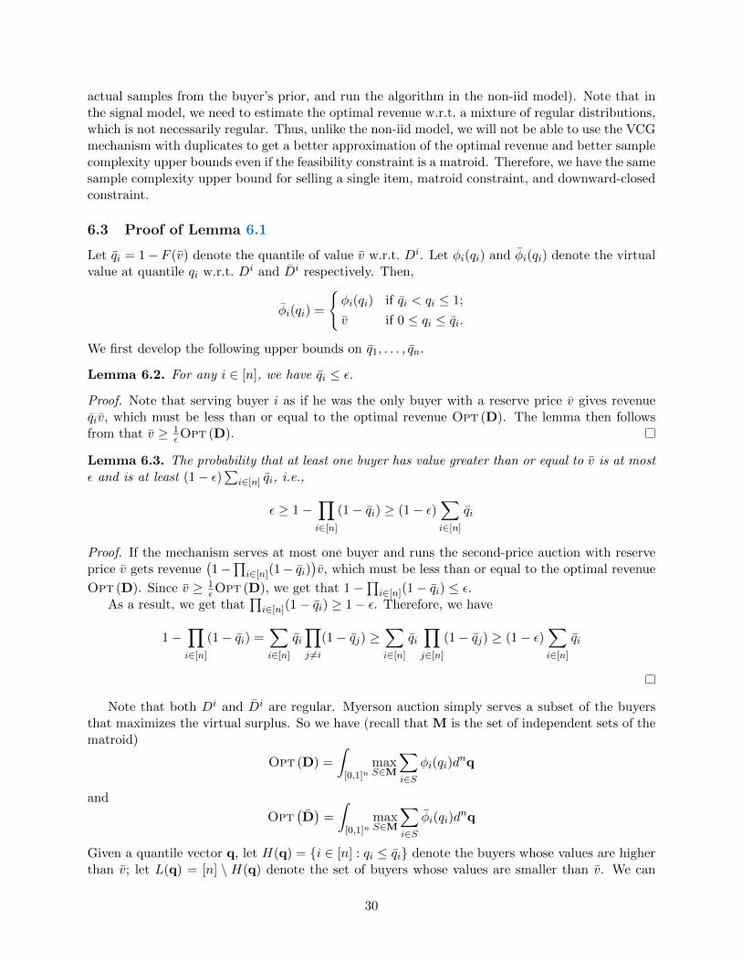
actual samples from the buyer’s prior, and run the algorithm in the non-iid model). Note that inthe signal model, we need to estimate the optimal revenue w.r.t. a mixture of regular distributions,which is not necessarily regular. Thus, unlike the non-iid model, we will not be able to use the VCGmechanism with duplicates to get a better approximation of the optimal revenue and better samplecomplexity upper bounds even if the feasibility constraint is a matroid. Therefore, we have the samesample complexity upper bound for selling a single item, matroid constraint, and downward-closedconstraint.

6.3 Proof of Lemma 6.1

Let qi = 1− F (v) denote the quantile of value v w.r.t. Di. Let φi(qi) and φi(qi) denote the virtualvalue at quantile qi w.r.t. Di and Di respectively. Then,

φi(qi) =

φi(qi) if qi < qi ≤ 1;

v if 0 ≤ qi ≤ qi.

We first develop the following upper bounds on q1, . . . , qn.

Lemma 6.2. For any i ∈ [n], we have qi ≤ ε.

Proof. Note that serving buyer i as if he was the only buyer with a reserve price v gives revenueqiv, which must be less than or equal to the optimal revenue Opt (D). The lemma then followsfrom that v ≥ 1

εOpt (D).

Lemma 6.3. The probability that at least one buyer has value greater than or equal to v is at mostε and is at least (1− ε)

∑i∈[n] qi, i.e.,

ε ≥ 1−∏i∈[n]

(1− qi) ≥ (1− ε)∑i∈[n]

qi

Proof. If the mechanism serves at most one buyer and runs the second-price auction with reserveprice v gets revenue

(1−

∏i∈[n](1− qi)

)v, which must be less than or equal to the optimal revenue

Opt (D). Since v ≥ 1εOpt (D), we get that 1−

∏i∈[n](1− qi) ≤ ε.

As a result, we get that∏i∈[n](1− qi) ≥ 1− ε. Therefore, we have

1−∏i∈[n]

(1− qi) =∑i∈[n]

qi∏j 6=i

(1− qj) ≥∑i∈[n]

qi∏j∈[n]

(1− qj) ≥ (1− ε)∑i∈[n]

qi

Note that both Di and Di are regular. Myerson auction simply serves a subset of the buyersthat maximizes the virtual surplus. So we have (recall that M is the set of independent sets of thematroid)

Opt (D) =

∫[0,1]n

maxS∈M

∑i∈S

φi(qi)dnq

and

Opt(D)

=

∫[0,1]n

maxS∈M

∑i∈S

φi(qi)dnq

Given a quantile vector q, let H(q) = i ∈ [n] : qi ≤ qi denote the buyers whose values are higherthan v; let L(q) = [n] \ H(q) denote the set of buyers whose values are smaller than v. We can

30

divide the revenue of Myerson’s optimal auction into two parts, the revenue from high value buyersand one from low value buyers. We will upper bound them separately.

Opt (D) ≤∫

[0,1]nmaxS∈H(q)

∑i∈S

φi(qi)dnq +

∫[0,1]n

maxS∈L(q)

∑i∈S

φi(qi)dnq

We will also divide the revenue of Myerson’s optimal auction w.r.t. the truncated distributions intotwo parts, the revenue when there are at least one high value buyer, and the revenue when allbuyers have low values.

Opt(D)

=

∫[0,1]n\

∏j [qj ,1]

maxS∈[n]

∑i∈S

φi(qi)dnq +

∫∏j [qj ,1]

maxS∈[n]

∑i∈S

φi(qi)dnq

It suffices to show∫[0,1]n\

∏j [qj ,1]

maxS∈[n]

∑i∈S

φi(qi)dnq ≥ (1− 2ε)

∫[0,1]n

maxS∈H(q)

∑i∈S

φi(qi)dnq (9)

and ∫∏j [qj ,1]

maxS∈[n]

∑i∈S

φi(qi)dnq ≥ (1− 2ε)

∫[0,1]n

maxS∈L(q)

∑i∈S

φi(qi)dnq (10)

Proof of (9): Note that for any i and any qi < qi, φi(qi) = v. Thus, the LHS of (9) is lowerbounded by ∫

[0,1]n\∏i[qi,1]

vdnq =(1−

∏i∈[n]

(1− qi))v ≥ (1− ε)

∑i∈[n]

qiv

where the inequality follows by Lemma 6.3. On the other hand, the RHS (omitting the 1 − 2εfactor) is upper bounded by∫

[0,1]nmaxS∈H(q)

∑i∈S

φi(qi)dnq ≤

∫[0,1]n

∑i∈H(q)

maxφi(qi), 0

dnq

≤∑i∈[n]

∫[0,qi]

maxφi(qi), 0dqi

Therefore, to show (9), it suffices to show that for every i ∈ [n],

qiv ≥ (1− ε)∫qi∈[0,qi]

maxφi(qi), 0

Let Ri(q) denote the revenue of a single-buyer auction with a reserve price that has quantile q w.r.t.Di. The LHS of the above is the revenue of a single-buyer auction with reserve price v w.r.t. Di,i.e., Ri(qi). The RHS is the maximum revenue of a single-buyer auction with a reserve price atleast v, i.e., maxq∈[0,qi]Ri(q). Note that Di’s being regular implies that Ri(q) is a concave functionover [0, 1] and Ri(1) ≥ 0. Thus, we have that Ri(qi) ≥ (1 − qi) maxq∈[0,qi]Ri(q). The inequalitythen follows by qi ≤ ε (Lemma 6.2).

31

Proof of (10): Note that for any q ∈∏j∈[n][qj , 1], we have L(q) = [n]. So we can rewrite the

LHS of (10) as follows.∫∏j [qj ,1]

maxS∈[n]

∑j∈S

φj(qj)dnq =

∫∏j [qj ,1]

maxS∈L(q)

∑j∈S

φj(qj)dnq

For any q−i ∈ [0, 1]n−1, any qi < qi ≤ q′i, suppose q = (qi,q−i) and q′ = (q′i,q−i). We have thatL(q) ⊂ L(q′), and for any i ∈ L(q), qi = q′i. Thus, maxS∈L(q)

∑j∈S φj(qj) ≤ maxS∈L(q′)

∑j∈S φj(q

′j).

Therefore, we have∫∏j [qj ,1]

maxS∈L(q)

∑j∈S

φj(qj)dnq ≥ (1− q1)

∫[0,1]×

∏nj=2[qj ,1]

maxS∈L(q)

∑j∈S

φj(qj)dnq

≥ (1− q1)(1− q2)

∫[0,1]2×

∏nj=3[qj ,1]

maxS∈L(q)

∑j∈S

φj(qj)dnq

≥ . . .

≥∏j∈[n]

(1− qj)∫

[0,1]nmaxS∈L(q)

∑j∈S

φj(qj)dnq

Finally, by Lemma 6.3, we have that∏j∈[n](1− qj) ≥ 1− ε. Putting together proves (10).

Acknowledgements

We would like to thank Matt Weinberg for the useful discussions about Revenue Monotonicity.This work was done in part while the authors were visiting the Simons Institute for the Theory ofComputing.

Bibliography

[1] Pablo Azar, Constantinos Daskalakis, Silvio Micali, and S Matthew Weinberg. Optimal andefficient parametric auctions. In Proceedings of the Twenty-Fourth Annual ACM-SIAM Sym-posium on Discrete Algorithms, pages 596–604. SIAM, 2013.

[2] Maria-Florina Balcan, Avrim Blum, Jason D Hartline, and Yishay Mansour. Reducing mech-anism design to algorithm design via machine learning. Journal of Computer and SystemSciences, 74(8):1245–1270, 2008.

[3] Sayan Bhattacharya, Elias Koutsoupias, Janardhan Kulkarni, Stefano Leonardi, Tim Rough-garden, and Xiaoming Xu. Near-optimal multi-unit auctions with ordered bidders. In Pro-ceedings of the Fourteenth ACM Conference on Electronic Commerce, EC ’13, pages 91–102,New York, NY, USA, 2013. ACM. ISBN 978-1-4503-1962-1. doi: 10.1145/2482540.2482555.URL http://doi.acm.org/10.1145/2482540.2482555.

[4] Jeremy Bulow and Paul Klemperer. Auction versus negotiations. American Economic Review,1996.

[5] Yang Cai and Constantinos Daskalakis. Extreme value theorems for optimal multidimensionalpricing. Games and Economic Behavior, 92:266–305, 2015.

32

http://doi.acm.org/10.1145/2482540.2482555

[6] Richard Cole and Tim Roughgarden. The sample complexity of revenue maximization. InSymposium on Theory of Computing, STOC 2014, New York, NY, USA, May 31 - June 03,2014, pages 243–252, 2014. doi: 10.1145/2591796.2591867. URL http://doi.acm.org/10.

1145/2591796.2591867.

[7] Peerapong Dhangwatnotai, Tim Roughgarden, and Qiqi Yan. Revenue maximization with asingle sample. Games and Economic Behavior, 2014.

[8] Shaddin Dughmi, Li Han, and Noam Nisan. Sampling and representation complexity of revenuemaximization. In Web and Internet Economics, pages 277–291. Springer, 2014.

[9] Edith Elkind. Designing and learning optimal finite support auctions. In Proceedings of theeighteenth annual ACM-SIAM symposium on Discrete algorithms, pages 736–745. Society forIndustrial and Applied Mathematics, 2007.

[10] Eyal Even-Dar, Jon Feldman, Yishay Mansour, and S Muthukrishnan. Position auctions withbidder-specific minimum prices. In Internet and Network Economics, pages 577–584. Springer,2008.

[11] Jason D Hartline and Tim Roughgarden. Simple versus optimal mechanisms. In Proceedingsof the 10th ACM conference on Electronic commerce, pages 225–234. ACM, 2009.

[12] Zhiyi Huang, Yishay Mansour, and Tim Roughgarden. Making the most of your samples.In Proceedings of the Sixteenth ACM Conference on Economics and Computation, EC ’15,Portland, OR, USA, June 15-19, 2015, pages 45–60, 2015.

[13] Sebastien Lahaie and David M Pennock. Revenue analysis of a family of ranking rules forkeyword auctions. In Proceedings of the 8th ACM conference on Electronic commerce, pages50–56. ACM, 2007.

[14] Stefano Leonardi and Tim Roughgarden. Prior-free auctions with ordered bidders. InProceedings of the Forty-fourth Annual ACM Symposium on Theory of Computing, STOC’12, pages 427–434, New York, NY, USA, 2012. ACM. ISBN 978-1-4503-1245-5. doi:10.1145/2213977.2214018. URL http://doi.acm.org/10.1145/2213977.2214018.

[15] Jamie Morgenstern and Tim Roughgarden. The pseudo-dimension of nearly-optimal auctions.In NIPS, page Forthcoming, 12 2015. URL papers/auction-pseudo.pdf.

[16] Roger B. Myerson. Optimal auction design. Mathematics of Operations Research, 6(1):58–73,1981.

[17] Michael Ostrovsky and Michael Schwarz. Reserve prices in internet advertising auctions: Afield experiment. In Proceedings of the 12th ACM conference on Electronic commerce, pages59–60. ACM, 2011.

[18] Bem Roberts, Dinan Gunawardena, Ian A Kash, and Peter Key. Ranking and tradeoffs insponsored search auctions. In Proceedings of the fourteenth ACM conference on Electroniccommerce, pages 751–766. ACM, 2013.

[19] Maurice Sion et al. On general minimax theorems. Pacific J. Math, 8(1):171–176, 1958.

[20] Balasubramanian Sivan and Vasilis Syrgkanis. Vickrey auctions for irregular distributions. InWeb and Internet Economics, pages 422–435. Springer, 2013.

33

http://doi.acm.org/10.1145/2591796.2591867

http://doi.acm.org/10.1145/2591796.2591867

http://doi.acm.org/10.1145/2213977.2214018

papers/auction-pseudo.pdf

[21] David RM Thompson and Kevin Leyton-Brown. Revenue optimization in the generalizedsecond-price auction. In Proceedings of the fourteenth ACM conference on Electronic commerce,pages 837–852. ACM, 2013.

34

y Christos-Alexandros Psomas z - arXiv · The Sample Complexity of Auctions with Side Information...

Documents

Transcript of y Christos-Alexandros Psomas z - arXiv · The Sample Complexity of Auctions with Side Information...