Alexandros Adam - University College London
218
Transcript of Alexandros Adam - University College London
UNIVERSITY COLLEGE LONDON
System Modelling and Optimisation
Studies of Fuel Cell Based micro-CHP
for Residential Energy Demand
Reduction
Alexandros Adam
A thesis submitted in ful�llment of the degree of
Doctor of Philosophy
Department of Chemical Engineering

Declaration of Authorship
I, Alexandros Adam con�rm that the work presented in this thesis is my own. Where
information has been derived from other sources, I con�rm that this has been indic-
ated in the thesis.
Signed:
Date:
1

Acknowledgements
I would like to express my deepest gratitude for the help and guidance received by my
supervisors Prof. Eric S. Fraga and Prof. Dan J.L Brett throughout my PhD: Eric
for introducing me to the amazing world of mathematical modelling but especially
for his approach of analysing situations. Dan for sharing his in depth knowledge of
the theory of fuel cells and for all the fun times in the Christmas parties.
There is a number of people that I would like to thank that helped me in various
ways. Maria-Christina, who is always close to me, encouraging me and supporting
my decisions. My parents Michalis and Anna for providing the continuous support
over the years of my studies. Also thank you to the people in the PPSE room,
Cristian, Asif, Shade for having great times in and outside the o�ce.
I would also like to thank Elisabeth Ness, a former Crest Nicholson employee, for the
interest she showed in my work. She happily organised a site visit for me to witness
a fuel cell micro-CHP system in operation in a Crest Nicholson test site in Epsom.
Finally, I would like to express my graditute to Georgios Mantas, a mathematics
teacher who was an inspirational �gure to me during my school times.
This research was made possible by EPSRC support for the London-Loughborough
Centre for Doctoral Research in Energy Demand, grant number EP/H009612/1 and
EPSRC funding support of the Electrochemical Innovation Lab via EP/G030995/1
and EP/I037024/1.
2
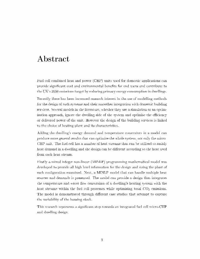
Abstract
Fuel cell combined heat and power (CHP) units used for domestic applications can
provide signi�cant cost and environmental bene�ts for end users and contribute to
the UK's 2050 emissions target by reducing primary energy consumption in dwellings.
Recently there has been increased research interest in the use of modelling methods
for the design of such systems and their smoother integration with domestic building
services. Several models in the literature, whether they use a simulation or an optim-
isation approach, ignore the dwelling side of the system and optimise the e�ciency
or delivered power of the unit. However the design of the building services is linked
to the choice of heating plant and its characteristics.
Adding the dwelling's energy demand and temperature constraints in a model can
produce more general results that can optimise the whole system, not only the micro-
CHP unit. The fuel cell has a number of heat streams that can be utilised to satisfy
heat demand in a dwelling and the design can be di�erent according to the heat used
from each heat stream.
Firstly a mixed integer non-linear (MINLP) programming mathematical model was
developed to provide all high level information for the design and sizing the plant of
each con�guration examined. Next, a MINLP model that can handle multiple heat
sources and demands is presented. The model can provide a design that integrates
the temperature and water �ow constraints of a dwelling's heating system with the
heat streams within the fuel cell processes while optimising total CO2 emissions.
The model is demonstrated through di�erent case studies that attempt to capture
the variability of the housing stock.
This research represents a signi�cant step towards an integrated fuel cell micro-CHP
and dwelling design.
3
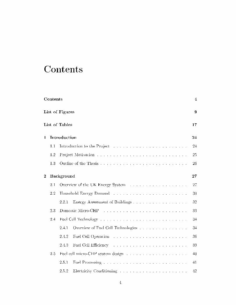
Contents
Contents 4
List of Figures 9
List of Tables 17
1 Introduction 24
1.1 Introduction to the Project . . . . . . . . . . . . . . . . . . . . . . . 24
1.2 Project Motivation . . . . . . . . . . . . . . . . . . . . . . . . . . . . 25
1.3 Outline of the Thesis . . . . . . . . . . . . . . . . . . . . . . . . . . . 26
2 Background 27
2.1 Overview of the UK Energy System . . . . . . . . . . . . . . . . . . 27
2.2 Household Energy Demand . . . . . . . . . . . . . . . . . . . . . . . 30
2.2.1 Energy Assessment of Buildings . . . . . . . . . . . . . . . . . 32
2.3 Domestic Micro-CHP . . . . . . . . . . . . . . . . . . . . . . . . . . 33
2.4 Fuel Cell Technology . . . . . . . . . . . . . . . . . . . . . . . . . . . 34
2.4.1 Overview of Fuel Cell Technologies . . . . . . . . . . . . . . . 34
2.4.2 Fuel Cell Operation . . . . . . . . . . . . . . . . . . . . . . . 36
2.4.3 Fuel Cell E�ciency . . . . . . . . . . . . . . . . . . . . . . . 39
2.5 Fuel cell micro-CHP system design . . . . . . . . . . . . . . . . . . . 40
2.5.1 Fuel Processing . . . . . . . . . . . . . . . . . . . . . . . . . . 41
2.5.2 Electricity Conditioning . . . . . . . . . . . . . . . . . . . . . 42
4
2.5.3 Heat Management . . . . . . . . . . . . . . . . . . . . . . . . 42
2.5.4 Controls . . . . . . . . . . . . . . . . . . . . . . . . . . . . . 43
2.6 Fuel cell micro-CHP Products . . . . . . . . . . . . . . . . . . . . . 43
2.7 Fuel cell micro-CHP Cost . . . . . . . . . . . . . . . . . . . . . . . . 44
2.8 Policy and Field Trials . . . . . . . . . . . . . . . . . . . . . . . . . . 46
2.9 Thermal Comfort and Heating Systems . . . . . . . . . . . . . . . . . 47
3 Previous Work 52
3.1 Modelling Fuel Cell micro-CHPs for domestic applications . . . . . . 52
3.1.1 Modelling Processes and Methods . . . . . . . . . . . . . . . . 53
3.1.2 Modelling Results . . . . . . . . . . . . . . . . . . . . . . . . 55
3.1.3 Concluding remarks . . . . . . . . . . . . . . . . . . . . . . . 56
4 Options for Residential Building Services Design Using Fuel Cell
Based Micro-CHP 57
4.1 The potential for integration with building services . . . . . . . . . . 57
4.2 Heat recovery in fuel cell micro-CHPs systems . . . . . . . . . . . . . 60
4.2.1 Heat recovery options in PEMFC systems . . . . . . . . . . . 62
4.2.1.1 Fuel Cell Stack . . . . . . . . . . . . . . . . . . . . . 62
4.2.1.2 Afterburner and Exhaust gases . . . . . . . . . . . . 62
4.2.1.3 Fuel Processor . . . . . . . . . . . . . . . . . . . . . 63
4.2.2 Heat recovery options in SOFC systems . . . . . . . . . . . . 63
4.2.3 PEMFC and SOFC di�erences in terms of heat recovery . . . 64
4.3 Design options for integration for fuel cell based micro-CHP . . . . . 64
5 Reference Building and Dwelling Energy Data 66
5.1 Reference Building . . . . . . . . . . . . . . . . . . . . . . . . . . . . 66
5.2 Dwelling Energy Data . . . . . . . . . . . . . . . . . . . . . . . . . . 71
5.2.1 House A - Part L Building . . . . . . . . . . . . . . . . . . . 73
5.2.1.1 UFH System . . . . . . . . . . . . . . . . . . . . . . 73
5
5.2.1.2 Radiator System . . . . . . . . . . . . . . . . . . . . 75
5.2.2 House B - Typical UK Dwelling . . . . . . . . . . . . . . . . . 77
5.2.2.1 UFH System . . . . . . . . . . . . . . . . . . . . . . 77
5.2.2.2 Radiator System . . . . . . . . . . . . . . . . . . . . 78
5.3 Datasets for Modelling . . . . . . . . . . . . . . . . . . . . . . . . . . 79
5.4 Summary of Results . . . . . . . . . . . . . . . . . . . . . . . . . . . 81
5.5 Concluding Remarks . . . . . . . . . . . . . . . . . . . . . . . . . . . 81
6 Model 1 - An MINLP model for high level evaluation of a SOFC
micro-CHP design in dwellings 82
6.1 Optimisation methods in energy systems . . . . . . . . . . . . . . . . 82
6.2 Problem Statement . . . . . . . . . . . . . . . . . . . . . . . . . . . . 84
6.3 Basis for the Model . . . . . . . . . . . . . . . . . . . . . . . . . . . . 84
6.4 Modelling Methodology . . . . . . . . . . . . . . . . . . . . . . . . . 85
6.4.1 Submodels . . . . . . . . . . . . . . . . . . . . . . . . . . . . . 85
6.4.1.1 Fuel Cell . . . . . . . . . . . . . . . . . . . . . . . . 85
6.4.1.2 Gas Boiler . . . . . . . . . . . . . . . . . . . . . . . 86
6.4.1.3 Thermal Storage Tank . . . . . . . . . . . . . . . . . 87
6.4.1.4 Thermal balance . . . . . . . . . . . . . . . . . . . . 88
6.4.1.5 Electricity balance . . . . . . . . . . . . . . . . . . . 88
6.4.1.6 Total System CO2 emissions . . . . . . . . . . . . . 89
6.5 Formulation and Solution Approach . . . . . . . . . . . . . . . . . . 89
6.5.1 Equations Transformation . . . . . . . . . . . . . . . . . . . . 92
6.6 Modelling Results . . . . . . . . . . . . . . . . . . . . . . . . . . . . . 95
6.6.1 Winter Day Analysis . . . . . . . . . . . . . . . . . . . . . . . 95
6.6.1.1 Case 1 . . . . . . . . . . . . . . . . . . . . . . . . . . 95
6.6.1.2 Case 2 . . . . . . . . . . . . . . . . . . . . . . . . . . 99
6.6.2 Summer day analysis . . . . . . . . . . . . . . . . . . . . . . . 104
6.6.2.1 Case 3 . . . . . . . . . . . . . . . . . . . . . . . . . . 104
6

6.6.2.2 Case 4 . . . . . . . . . . . . . . . . . . . . . . . . . . 108
6.6.3 Combined 48-hour Dataset . . . . . . . . . . . . . . . . . . . 114
6.6.3.1 Case 5 . . . . . . . . . . . . . . . . . . . . . . . . . . 114
6.6.3.2 Case 6 . . . . . . . . . . . . . . . . . . . . . . . . . . 118
6.6.4 Summary of Results . . . . . . . . . . . . . . . . . . . . . . . 123
6.7 Discussion and Critical Analysis . . . . . . . . . . . . . . . . . . . . . 124
6.8 Limitations of the study . . . . . . . . . . . . . . . . . . . . . . . . . 126
6.9 Concluding Remarks . . . . . . . . . . . . . . . . . . . . . . . . . . . 127
7 Model 2 - An MINLP model for PEMFC based micro-CHP design
in dwellings 128
7.1 Problem Statement . . . . . . . . . . . . . . . . . . . . . . . . . . . . 128
7.2 Basis for the PEMFC Model . . . . . . . . . . . . . . . . . . . . . . . 129
7.3 Modelling Methodology . . . . . . . . . . . . . . . . . . . . . . . . . 129
7.3.1 Submodels . . . . . . . . . . . . . . . . . . . . . . . . . . . . . 132
7.3.1.1 Fuel Cell Stack . . . . . . . . . . . . . . . . . . . . . 132
7.3.1.2 Reformer . . . . . . . . . . . . . . . . . . . . . . . . 133
7.3.1.3 Afterburner . . . . . . . . . . . . . . . . . . . . . . 135
7.3.1.4 Gas Boiler . . . . . . . . . . . . . . . . . . . . . . . 136
7.3.1.5 Thermal Storage Tank . . . . . . . . . . . . . . . . . 138
7.3.1.6 Pipe network and Heat Emitters . . . . . . . . . . . 140
7.3.1.7 Electricity Energy Balance . . . . . . . . . . . . . . 142
7.3.1.8 Total System CO2 emissions . . . . . . . . . . . . . 142
7.4 Formulation and Solution Approach . . . . . . . . . . . . . . . . . . 143
7.5 Modelling Results . . . . . . . . . . . . . . . . . . . . . . . . . . . . . 148
7.5.1 Part L Dwelling Designed with UFH . . . . . . . . . . . . . . 148
7.5.1.1 Case 1 . . . . . . . . . . . . . . . . . . . . . . . . . . 148
7.5.1.2 Case 2 . . . . . . . . . . . . . . . . . . . . . . . . . . 156
7.5.1.3 Variation 1 - The e�ect of applying a di�erent tem-
perature constraint on the storage model . . . . . . 163
7
7.5.1.4 Comparative Results . . . . . . . . . . . . . . . . . 165
7.5.2 Part L Dwelling Designed with Radiators . . . . . . . . . . . 168
7.5.2.1 Case 3 . . . . . . . . . . . . . . . . . . . . . . . . . . 169
7.5.2.2 Variation 2 - The e�ect of the minimum modulation
of the gas boiler . . . . . . . . . . . . . . . . . . . . 174
7.5.2.3 Case 4 . . . . . . . . . . . . . . . . . . . . . . . . . . 176
7.5.2.4 Comparative Results . . . . . . . . . . . . . . . . . 186
7.5.3 Part L Dwelling - Electricity Exporting Scenarios . . . . . . . 187
7.5.3.1 Case 5 . . . . . . . . . . . . . . . . . . . . . . . . . . 188
7.5.3.2 Case 6 . . . . . . . . . . . . . . . . . . . . . . . . . . 189
7.5.4 House B -Typical UK Dwelling . . . . . . . . . . . . . . . . . 191
7.5.4.1 Case 7 . . . . . . . . . . . . . . . . . . . . . . . . . . 191
7.6 Discussion and Critical Analysis . . . . . . . . . . . . . . . . . . . . . 194
7.7 Limitations of the study . . . . . . . . . . . . . . . . . . . . . . . . . 198
7.8 Concluding Remarks . . . . . . . . . . . . . . . . . . . . . . . . . . . 199
8 Conclusions and Future Directions 200
8.1 Summary of Contribution . . . . . . . . . . . . . . . . . . . . . . . . 200
8.2 Implications for fuel cell micro-CHP system design . . . . . . . . . . 201
8.3 Recommendations for future work . . . . . . . . . . . . . . . . . . . . 202
Bibliography 204
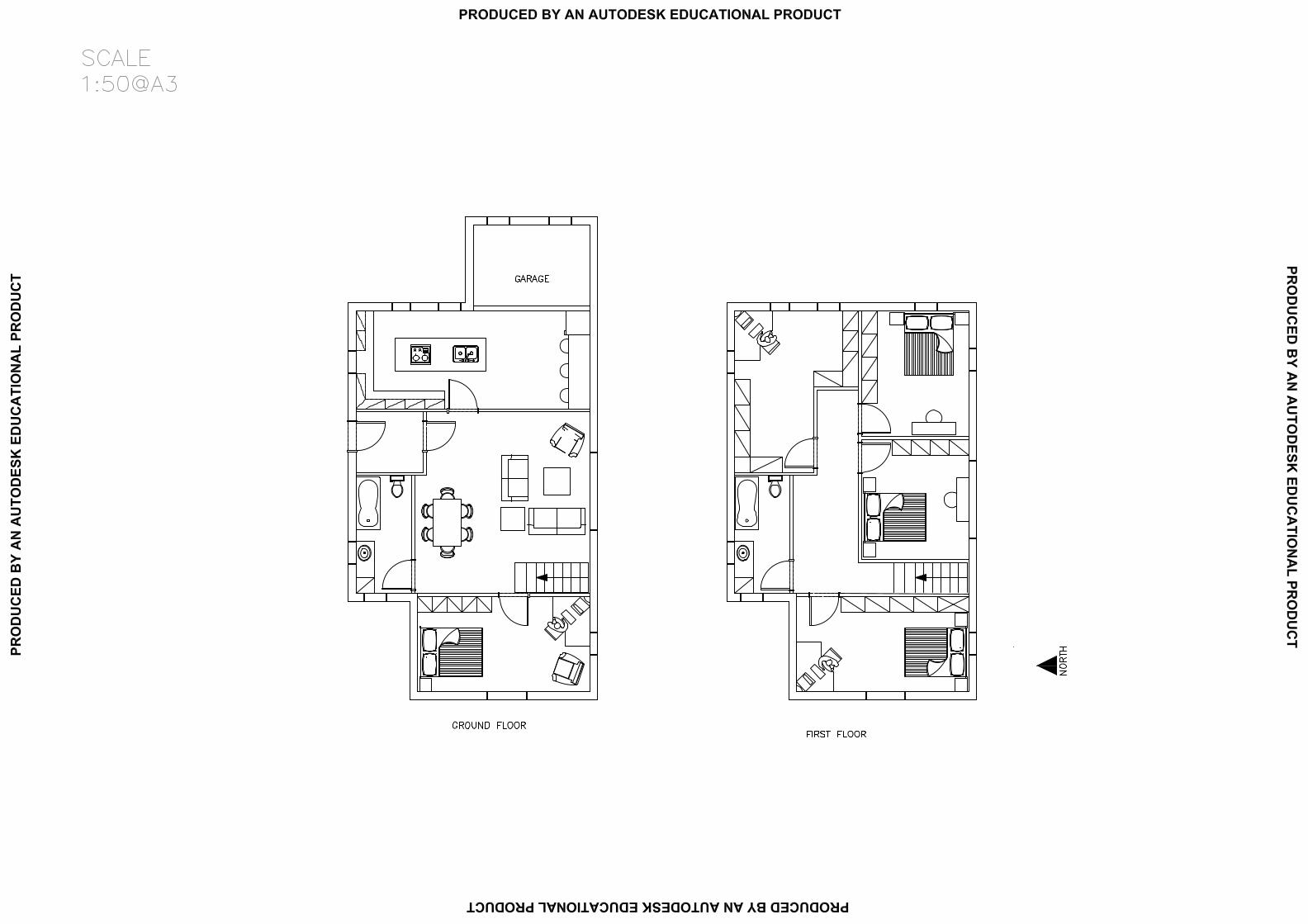
A Reference House Architectural Drawings 216
8
List of Figures
2.1.1 Production and Consumption of Primary Fuels in the UK in 2013 (
[48]) . . . . . . . . . . . . . . . . . . . . . . . . . . . . . . . . . . . . 28
2.1.2 Energy Consumption by fuel in the UK from 1970 to 2013 ( [49]) . . 28
2.1.3 Sankey Diagram of UK Energy System in 2013 ([43]) . . . . . . . . . 29
2.2.1 UK Domestic sector fuel mixture ([46]) . . . . . . . . . . . . . . . . . 31
2.2.2 UK domestic �nal energy consumption by end user since 1970 ([46]) 32
2.3.1 Simpli�ed diagram of a CHP system showing energy �ows . . . . . . 34
2.4.1 Fuel Cell Basic Operation ( [65]) . . . . . . . . . . . . . . . . . . . . 35
2.4.2 Graph showing the voltage of an average PEMFC fuel cell against the
current density, illustrating the energy losses that occur . . . . . . . 38
2.4.3 Graph showing the power output of an average PEMFC fuel cell
against the current density . . . . . . . . . . . . . . . . . . . . . . . . 39
2.4.4 Graph showing the electrical, thermal and total e�ciency of an SOFC
in relation to the load factor [73] . . . . . . . . . . . . . . . . . . . . 40
2.5.1 Schematic Diagram of fuel cell micro-CHP components ([125]) . . . 41
2.6.1 Images of fuel cell micro-CHP products [34, 113] . . . . . . . . . . . 44
2.9.1 Images of Radiator and Under�oor Heating System ([112],[124]) . . 49
2.9.2 Simpli�ed Schematic of Combi Boiler . . . . . . . . . . . . . . . . . . 50
2.9.3 Simpli�ed Schematic of Gas Fired Boiler and DHW Storage Tank . . 51
2.9.4 Schematic showing the operation of a low loss header illustrating
primary and secondary circuits [2]. . . . . . . . . . . . . . . . . . . . 51
4.1.1 Storage Tank for use in a micro-CHP system ([31]) . . . . . . . . . . 58
9
4.1.2 Simpli�ed Schematic Diagram of Fuel Cell micro-CHP system - Con-
�guration 1 - Thermal Storage Tank Present . . . . . . . . . . . . . . 59
4.1.3 Simpli�ed Schematic Diagram of Fuel Cell micro-CHP system - Con-
�guration 2 - Without Thermal Storage Tank . . . . . . . . . . . . . 59
4.1.4 Simpli�ed Schematic Diagram of Fuel Cell micro-CHP system - Con-
�guration 3 - Fuel cell serves DHW . . . . . . . . . . . . . . . . . . . 60
4.2.1 Schematic illustration of a PEMFC micro-CHP system showing op-
tions for heat recovery. [2] . . . . . . . . . . . . . . . . . . . . . . . . 61
4.2.2 Schematic illustration of a SOFC micro-CHP system showing options
for heat recovery. . . . . . . . . . . . . . . . . . . . . . . . . . . . . . 64
4.3.1 Schematic diagram of fuel cell micro-CHP design for a dwelling . . . 65
5.1.1 Daily pro�le of the occupancy ratio (reproduced from IES VE [87]) . 68
5.1.2 Daily pro�le showing the internal set-point temperature (reproduced
from IES VE [87]) . . . . . . . . . . . . . . . . . . . . . . . . . . . . 68
5.1.3 Image showing the structure of the 3D model. This image is used
to illustrate the process of creating the structure of the model which
is using series of rectangular blocks to develop the �nal shape of the
building. . . . . . . . . . . . . . . . . . . . . . . . . . . . . . . . . . . 70
5.1.4 Image showing the exterior of the 3D model . . . . . . . . . . . . . . 70
5.2.1 Graph representing the 24-hour heat demand for DHW pattern for
the reference dwelling. The graph shows the relation between the
occupancy, which is high in the morning and in the evening hours,
and the DHW demand. . . . . . . . . . . . . . . . . . . . . . . . . . 72
5.2.2 Graph representing the weekly electricity demand for House A. This
weekly electricity pattern repeats throughout the year and peaks in
the weekends. . . . . . . . . . . . . . . . . . . . . . . . . . . . . . . . 73
5.2.3 Graph representing the demand of the base case for House A served
by an under�oor heating system . . . . . . . . . . . . . . . . . . . . . 74
5.2.4 Graph representing the winter space heating demand of the base case
for House A served by a under�oor heating system on a 24-hour seg-
ment of the complete annual dataset . . . . . . . . . . . . . . . . . . 75
5.2.5 Graph representing the demand of the base case for House A served
by a radiator system . . . . . . . . . . . . . . . . . . . . . . . . . . . 76
10
5.2.6 Graph representing the winter heating demand of the base case for
House A served by a radiator system on a 24-hour segment of the
complete 8760 hour dataset . . . . . . . . . . . . . . . . . . . . . . . 77
5.2.7 Graph representing the demand of the base case for House B served
by an under�oor heating system . . . . . . . . . . . . . . . . . . . . . 78
5.2.8 Annual variation of heating load for House B . . . . . . . . . . . . . 79
6.3.1 Basic structure of the model . . . . . . . . . . . . . . . . . . . . . . . 85
6.4.1 Thermal Storage Tank energy �ows in model 1 . . . . . . . . . . . . 88
6.5.1 Linearisation of the electrical e�ciency ηfc,ele(t) of an SOFC showing
cutting points . . . . . . . . . . . . . . . . . . . . . . . . . . . . . . 94
6.5.2 Linearisation of the thermal e�ciency ηfc,heat(t) of an SOFC showing
cutting points . . . . . . . . . . . . . . . . . . . . . . . . . . . . . . . 94
6.6.1 Graph representing the load factor of the fuel cell micro-CHP and
auxiliary boiler for Case 1 . . . . . . . . . . . . . . . . . . . . . . . . 96
6.6.2 Graph representing the electrical and thermal e�ciencies of the fuel
cell micro-CHP for Case 1 . . . . . . . . . . . . . . . . . . . . . . . . 97
6.6.3 Graph representing the electricity output of the fuel cell micro-CHP
and grid electricity for Case 1 . . . . . . . . . . . . . . . . . . . . . . 98
6.6.4 Graph representing the heat output of the fuel cell micro-CHP and
auxiliary gas boiler for Case 1 . . . . . . . . . . . . . . . . . . . . . . 99
6.6.5 Graph representing the load factor of the fuel cell micro-CHP and
auxiliary boiler for Case 2 . . . . . . . . . . . . . . . . . . . . . . . . 100
6.6.6 Graph representing the electrical and thermal e�ciencies of the fuel
cell micro-CHP and auxiliary boiler for Case 2 . . . . . . . . . . . . . 101
6.6.7 Graph representing the electricity output of the fuel cell micro-CHP
and grid electricity for Case 2 . . . . . . . . . . . . . . . . . . . . . . 101
6.6.8 Graph representing the heat output of the fuel cell micro-CHP and
auxiliary boiler for Case 2 . . . . . . . . . . . . . . . . . . . . . . . . 102
6.6.9 Graph representing the heat output from the thermal storage tank to
the house for Case 2 . . . . . . . . . . . . . . . . . . . . . . . . . . . 103
6.6.10 Graph representing the heat content of the thermal storage tank for
Case 2 . . . . . . . . . . . . . . . . . . . . . . . . . . . . . . . . . . . 104
11
6.6.11 Graph representing the load factor of the fuel cell micro-CHP and
auxiliary boiler for Case 3 . . . . . . . . . . . . . . . . . . . . . . . . 105
6.6.12 Graph representing the electrical and thermal e�ciencies of the fuel
cell micro-CHP for Case 3 . . . . . . . . . . . . . . . . . . . . . . . . 106
6.6.13 Graph representing the electricity output of the fuel cell micro-CHP
and grid electricity for Case 3 . . . . . . . . . . . . . . . . . . . . . . 107
6.6.14 Graph representing the heat output of the fuel cell micro-CHP and
auxiliary boiler for Case 3 . . . . . . . . . . . . . . . . . . . . . . . . 108
6.6.15 Graph representing the load factor of the fuel cell micro-CHP and
auxiliary boiler for Case 4 . . . . . . . . . . . . . . . . . . . . . . . . 109
6.6.16 Graph representing the electrical and thermal e�ciencies of the fuel
cell micro-CHP and auxiliary boiler for Case 4 . . . . . . . . . . . . . 110
6.6.17 Graph representing the electricity output of the fuel cell micro-CHP
and grid electricity for Case 4 . . . . . . . . . . . . . . . . . . . . . . 111
6.6.18 Graph representing the heat output of the fuel cell micro-CHP and
auxiliary boiler for Case 4 . . . . . . . . . . . . . . . . . . . . . . . . 112
6.6.19 Graph representing the heat output from the thermal storage tank
to the house for Case 4 . . . . . . . . . . . . . . . . . . . . . . . . . . 113
6.6.20 Graph representing the heat content of the thermal storage tank for
Case 4 . . . . . . . . . . . . . . . . . . . . . . . . . . . . . . . . . . . 114
6.6.21 Graph representing the load factor of the fuel cell micro-CHP and
auxiliary boiler for Case 5 . . . . . . . . . . . . . . . . . . . . . . . . 116
6.6.22 Graph representing the electrical and thermal e�ciencies of the fuel
cell micro-CHP for Case 5 . . . . . . . . . . . . . . . . . . . . . . . . 117
6.6.23 Graph representing the electricity output of the fuel cell micro-CHP
and grid electricity for Case 5 . . . . . . . . . . . . . . . . . . . . . . 117
6.6.24 Graph representing the heat output of the fuel cell micro-CHP and
auxiliary boiler for Case 5 . . . . . . . . . . . . . . . . . . . . . . . . 118
6.6.25 Graph representing the load factor of the fuel cell micro-CHP and
auxiliary boiler for Case 6 . . . . . . . . . . . . . . . . . . . . . . . . 119
6.6.26 Graph representing the electrical and thermal e�ciencies of the fuel
cell micro-CHP for Case 6 . . . . . . . . . . . . . . . . . . . . . . . . 120
12
6.6.27 Graph representing the electricity output of the fuel cell micro-CHP
and grid electricity for System 6 . . . . . . . . . . . . . . . . . . . . . 120
6.6.28 Graph representing the heat output of the fuel cell micro-CHP and
auxiliary boiler for Case 6 . . . . . . . . . . . . . . . . . . . . . . . . 121
6.6.29 Graph representing the heat output from the thermal storage tank
to the house for Case 6 . . . . . . . . . . . . . . . . . . . . . . . . . . 122
6.6.30 Graph representing the heat content of the thermal storage tank for
Case 6 . . . . . . . . . . . . . . . . . . . . . . . . . . . . . . . . . . . 123
6.6.31 Graph representing the CO2 emissions of all systems presented in
Chapter 6 . . . . . . . . . . . . . . . . . . . . . . . . . . . . . . . . . 124
7.3.1 PEMFC based micro-CHP model schematic diagram . . . . . . . . . 131
7.3.2 Schematic of the fuel cell stack showing mass and energy �ows . . . . 132
7.3.3 Schematic of the reformer showing mass and energy �ows . . . . . . 134
7.3.4 Schematic of the afterburner showing mass and energy �ows . . . . . 135
7.3.5 Natural Gas Boiler Schematic showing mass and energy �ows . . . . 137
7.5.1 Schematic diagram representing the optimum design con�guration for
case 1 . . . . . . . . . . . . . . . . . . . . . . . . . . . . . . . . . . . 149
7.5.2 Graph representing how the system satis�es heating demand utilising
heat from the two fuel cell heat exchangers and the natural gas boiler
for Case 1 . . . . . . . . . . . . . . . . . . . . . . . . . . . . . . . . . 150
7.5.3 Graph representing how the system satis�es DHW demand utilising
heat from the two fuel cell heat exchangers and the natural gas boiler
for Case 1 . . . . . . . . . . . . . . . . . . . . . . . . . . . . . . . . . 151
7.5.4 Graph showing the utilisation factor of hydrogen at the fuel cell for
Case 1. . . . . . . . . . . . . . . . . . . . . . . . . . . . . . . . . . . . 152
7.5.5 Graph showing the available heat from the afterburner and the re-
covered heat at the reformer for Case 1 . . . . . . . . . . . . . . . . 153
7.5.6 Graph showing the individual system temperatures over a winter 24
hour period for Case 1 . . . . . . . . . . . . . . . . . . . . . . . . . . 154
7.5.7 Graph showing the �nal space heating and DHW temperatures for
Case 1 . . . . . . . . . . . . . . . . . . . . . . . . . . . . . . . . . . 154
13
7.5.8 Graph showing the total water �ow from the heating header to the
UFH manifold for Case 1. The water �ow is 0 in the summer months
when space heating demand is 0. . . . . . . . . . . . . . . . . . . . . 155
7.5.9 Graph showing the fuel cell electricity generation and the electricity
from the grid for Case 1 . . . . . . . . . . . . . . . . . . . . . . . . . 156
7.5.10 Schematic diagram representing the optimum design con�guration
for case 2 showing the TST in addition to the other units and its
connections to the system . . . . . . . . . . . . . . . . . . . . . . . . 157
7.5.11 Graph representing the electricity output of the fuel cell micro-CHP
for Case 2 . . . . . . . . . . . . . . . . . . . . . . . . . . . . . . . . . 158
7.5.12 Graph representing the heat extracted from the fuel cell and where
this heat is delivered in the dwelling on a winter day for Case 2 . . . 159
7.5.13 Graph representing the heat extracted from the fuel cell and where
this heat is delivered in the dwelling on a summer day for Case 2 . . 160
7.5.14 Graph representing the heat input and output of the TST for Case 2 161
7.5.15 Graph representing the variation of water temperature in the TST
for Case 2 . . . . . . . . . . . . . . . . . . . . . . . . . . . . . . . . . 162
7.5.16 Graph showing the individual system temperatures over a winter 24
hour period for Case 2 . . . . . . . . . . . . . . . . . . . . . . . . . . 162
7.5.17 Graph showing the �nal total system temperatures for space heating
and DHW over a 288 hour period for Case 2 . . . . . . . . . . . . . . 163
7.5.18 Graph representing the variation of water temperature in the TST
for Case 2b . . . . . . . . . . . . . . . . . . . . . . . . . . . . . . . . 165
7.5.19 Graph showing the total return system temperatures over a winter
24 hour period for Cases 1 and 2 . . . . . . . . . . . . . . . . . . . . 167
7.5.20 Graph showing the total boiler operation over the whole year period
for Cases 1 and 2 . . . . . . . . . . . . . . . . . . . . . . . . . . . . . 168
7.5.21 Schematic diagram representing the optimum design con�guration
for case 3 . . . . . . . . . . . . . . . . . . . . . . . . . . . . . . . . . 170
7.5.22 Graph showing the supply temperatures of the fuel cell cooling circuit
and afterburner heat exchangers over a period of 48 hours for Case 3.
Additionally the heat output of each heat exchanger to space heating
is shown on the right axis . . . . . . . . . . . . . . . . . . . . . . . . 172
14
7.5.23 Graph showing the total system temperatures over the �rst 48 hour
period for Case 3. At times of 0 demand, the temperature variable
takes also the 0 value as it can be seen for the space heating supply
and return temperature. . . . . . . . . . . . . . . . . . . . . . . . . 173
7.5.24 Graph showing total water �ow rates over the whole 288 hour period
for Case 3 . . . . . . . . . . . . . . . . . . . . . . . . . . . . . . . . . 174
7.5.25 Graph showing the load factor of the gas boiler over the whole 288
hour period for all cases after altering the minimum modulation limit 175
7.5.26 Graph representing the electricity generation of the fuel cell on a
winter and on a summer day for Case 4 . . . . . . . . . . . . . . . . 177
7.5.27 Graph representing the heat extracted from the afterburner and the
heat recovered from the reformer for Case 4 . . . . . . . . . . . . . . 178
7.5.28 Graph representing the heat output of each plant delivered to the
space heating circuit on an annual basis for Case 4. The graph shows
the output of the gas boiler is supplementary to the fuel cell which is
sized to cover most heat demand . . . . . . . . . . . . . . . . . . . . 179
7.5.29 Graph representing the heat output of each plant delivered to the
DHW circuit on an annual basis for Case 4 . . . . . . . . . . . . . . 180
7.5.30 Graph representing the heat extracted from the fuel cell and where
this heat is delivered in the dwelling on a winter day for Case 4 . . . 181
7.5.31 Graph representing the heat extracted from the fuel cell and where
this heat is delivered in the dwelling on a summer day for Case 4 . . 182
7.5.32 Graph representing the heat input and output of the TST for Case 4 183
7.5.33 Graph representing the variation of water temperature in the TST
for Case 4 . . . . . . . . . . . . . . . . . . . . . . . . . . . . . . . . . 184
7.5.34 Graph representing the supply temperature and heat released from
the fuel cell cooling circuit to the space heating pipe circuit for Case 4. 185
7.5.35 Graph representing the supply temperature and heat released from
the afterburner circuit to the space heating pipe circuit for Case 4. . 186
7.5.36 Breakdown of emissions caused by altering the limit of exported
electricity to the grid for case 5. Emissions reduce as the limit increases189
7.5.37 Graph representing the heat input and output of the TST for Case 6.190
15
7.5.38 Graph representing the heat output of each plant delivered to the
space heating circuit on an annual basis for Case 7. The graph shows
the output of the fuel cell is supplementary to the gas boiler which is
sized to cover most heat demand. . . . . . . . . . . . . . . . . . . . . 192
7.5.39 Graph representing the heat output of each plant delivered to the
DHW on an annual basis for Case 7. . . . . . . . . . . . . . . . . . 193
7.5.40 Graph representing the variation of water temperature in the TST
for Case 7 . . . . . . . . . . . . . . . . . . . . . . . . . . . . . . . . . 194
16
List of Tables
2.1 Comparison of Fuel Cell Technologies ([122]) . . . . . . . . . . . . . . 36
2.2 Fuel Cell CHP 2014 cost estimates (source [78]) . . . . . . . . . . . . 45
2.3 CHP 2012 cost estimates (source [110]) . . . . . . . . . . . . . . . . . 45
2.4 Recommended internal design temperatures for dwellings in the UK
as recommended by CIBSE ([37]) . . . . . . . . . . . . . . . . . . . . 47
2.5 Comparison of common heating services design con�gurations. ([36,
38, 96] ) . . . . . . . . . . . . . . . . . . . . . . . . . . . . . . . . . . 50
5.1 U Values of Houses A and B used as input in the building information
modelling software . . . . . . . . . . . . . . . . . . . . . . . . . . . . 67
5.2 Internal temperatures for selected dwelling . . . . . . . . . . . . . . 69
5.3 Reference Building emissions for House A as used in Model 1 . . . . 81
5.4 Reference Building emissions for Houses A and B as used in Model 2
for the 288-hour datasets . . . . . . . . . . . . . . . . . . . . . . . . 81
6.1 Details of model's parameters. . . . . . . . . . . . . . . . . . . . . . . 90
6.2 Variable low and upper bounds for Model 1. . . . . . . . . . . . . . . 90
6.3 Optimisation variables for Case 1 and comparison with reference build-
ing . . . . . . . . . . . . . . . . . . . . . . . . . . . . . . . . . . . . 96
6.4 Optimisation variables for Case 2 and comparison with reference build-
ing . . . . . . . . . . . . . . . . . . . . . . . . . . . . . . . . . . . . 100
6.5 Optimisation variables for Case 3 and comparison with reference build-
ing . . . . . . . . . . . . . . . . . . . . . . . . . . . . . . . . . . . . 105
6.6 Optimisation variables for Case 4 and comparison with reference build-
ing . . . . . . . . . . . . . . . . . . . . . . . . . . . . . . . . . . . . 108
17
6.7 Optimisation variables for Case 5 and comparison with reference build-
ing . . . . . . . . . . . . . . . . . . . . . . . . . . . . . . . . . . . . 115
6.8 Optimisation variables for Case 6 and comparison with reference build-
ing . . . . . . . . . . . . . . . . . . . . . . . . . . . . . . . . . . . . 118
6.9 Summary of CO2 emissions of all cases examined using model 1 . . 123
7.1 Parameters used in model 2 . . . . . . . . . . . . . . . . . . . . . . . 145
7.2 Bounds used for variables in model 2. When the symbol �/� is used
the values for the di�erent heating systems used in the analysis are
indicated. . . . . . . . . . . . . . . . . . . . . . . . . . . . . . . . . . 146
7.3 Annual heat contribution for each source for case 1 . . . . . . . . . . 149
7.4 Annual heat contribution for each source for case 2 . . . . . . . . . . 157
7.5 Annual heat contribution for each source for Case 2b . . . . . . . . . 164
7.6 Summary of results for cases l and 2 . . . . . . . . . . . . . . . . . . 165
7.7 Overview of system characteristics for cases 1 and 2 . . . . . . . . . . 166
7.8 Annual heat contribution for each source for case 3 . . . . . . . . . . 171
7.9 CO2 emission of each system after altering the minimum modulation
level of the gas boiler . . . . . . . . . . . . . . . . . . . . . . . . . . . 175
7.10 Annual heat contribution for each source for case 4 . . . . . . . . . . 176
7.11 Summary of results for cases 3 and 4 . . . . . . . . . . . . . . . . . . 187
7.12 Overview of system characteristics for cases 3 and 4 . . . . . . . . . . 187
7.13 Overview of system characteristics for case 5 . . . . . . . . . . . . . . 188
7.14 Overview of system characteristics for case 6 . . . . . . . . . . . . . . 189
7.15 Annual heat contribution from each source for case 7 . . . . . . . . 191
18

19
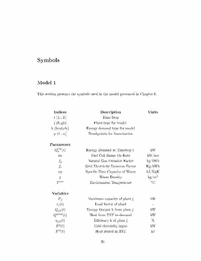
Symbols
Model 1
This section presents the symbols used in the model presented in Chapter 6.
Indices Description Units
t (1...T) Time Step
j (fc,gb) Plant type for model
k (heat,ele) Energy demand type for model
p (1...n) Breakpoints for linearisation
Parameters
Qreqk (t) Energy Demand at Timestep t kW
ra Fuel Cell Ramp Up Rate kW/sec
fg Natural Gas Emission Factor kg/kWh
fe Grid Electricity Emission Factor Kg/kWh
cp Speci�c Heat Capacity of Water kJ/KgK
ρ Water Density kg/m3
T env Environment Temperature oC
Variables
P j Maximum capacity of plant j kW
rj(t) Load factor of plant -
Qj,k(t) Energy Output k from plant j kW
Qstout(t) Heat from TST to demand kW
ηj,k(t) E�ciency k of plant j %
Eg(t) Grid electricity input kW
Est(t) Heat stored in TST kJ
20
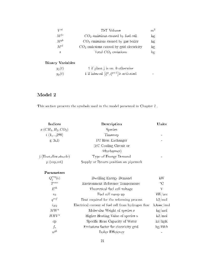
V st TST Volume m3
Mfc CO2 emissions caused by fuel cell kg
Mgb CO2 emissions caused by gas boiler kg
M el CO2 emissions caused by grid electricity kg
z Total CO2 emissions kg
Binary Variables
yj(t) 1 if plant j is on, 0 otherwise -
yp(t) 1 if interval[ξp, ξp+1
]is activated -
Model 2
This section presents the symbols used in the model presented in Chapter 7 .
Indices Description Units
s (CH4, H2, CO2) Species -
t (1,...,288) Timestep -
g (h,l) FC Heat Exchanger -
(FC Cooling Circuit or
Afterburner)
j (Heat,dhw,sto,ele) Type of Energy Demand -
p (sup,ret) Supply or Return position on pipework -
Parameters
Qreqj (t) Dwelling Energy Demand kW
T env Environment Reference Temperature °C
Eth Theoretical fuel cell voltage V
ra Fuel cell ramp up kW/sec
qref Heat required for the reforming process kJ/mol
iH2 Electrical current of fuel cell from hydrogen �ow kAsec/mol
MW s Molecular Weight of species s kg/mol
HHV s Higher Heating Value of species s kJ/mol
cp Speci�c Heat Capacity of Water kJ/kgK
fe Emissions factor for electricity grid kg/kWh
ngb Boiler E�ciency -
21
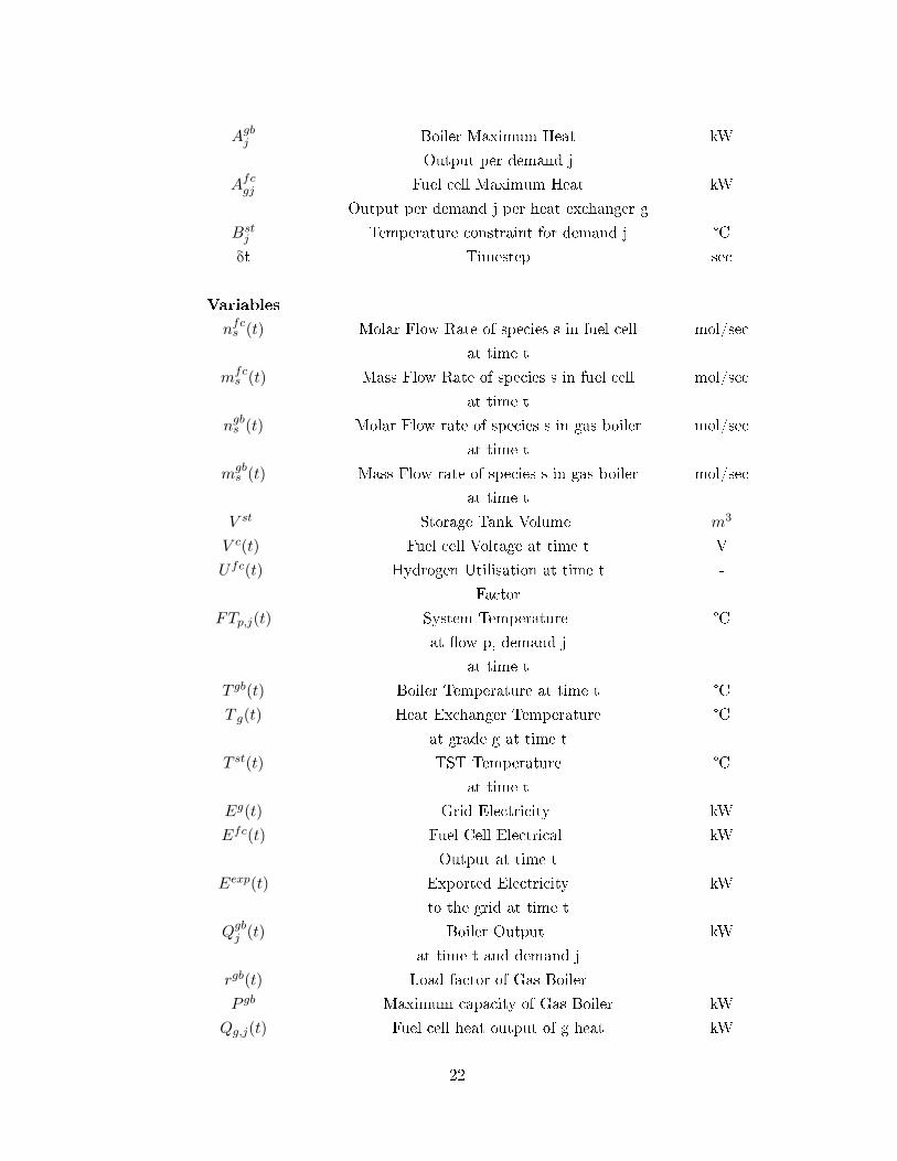
Agbj Boiler Maximum Heat kW
Output per demand j
Afcgj Fuel cell Maximum Heat kW
Output per demand j per heat exchanger g
Bstj Temperature constraint for demand j °C
δt Timestep sec
Variables -
nfcs (t) Molar Flow Rate of species s in fuel cell mol/sec
at time t
mfcs (t) Mass Flow Rate of species s in fuel cell mol/sec
at time t
ngbs (t) Molar Flow rate of species s in gas boiler mol/sec
at time t
mgbs (t) Mass Flow rate of species s in gas boiler mol/sec
at time t
V st Storage Tank Volume m3
V c(t) Fuel cell Voltage at time t V
Ufc(t) Hydrogen Utilisation at time t -
Factor
FTp,j(t) System Temperature °C
at �ow p, demand j
at time t
T gb(t) Boiler Temperature at time t °C
T g(t) Heat Exchanger Temperature °C
at grade g at time t
T st(t) TST Temperature °C
at time t
Eg(t) Grid Electricity kW
Efc(t) Fuel Cell Electrical kW
Output at time t
Eexp(t) Exported Electricity kW
to the grid at time t
Qgbj (t) Boiler Output kW
at time t and demand j
rgb(t) Load factor of Gas Boiler -
P gb Maximum capacity of Gas Boiler kW
Qg,j(t) Fuel cell heat output of g heat kW
22
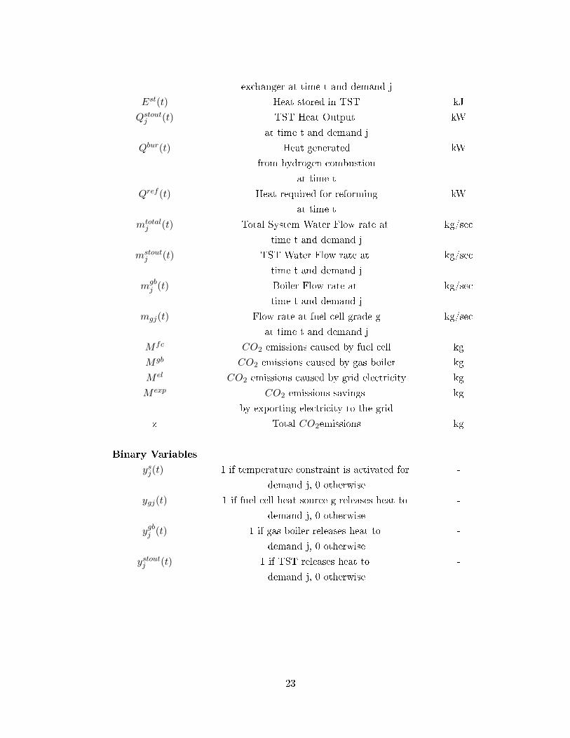
exchanger at time t and demand j
Est(t) Heat stored in TST kJ
Qstoutj (t) TST Heat Output kW
at time t and demand j
Qbur(t) Heat generated kW
from hydrogen combustion
at time t
Qref (t) Heat required for reforming kW
at time t
mtotalj (t) Total System Water Flow rate at kg/sec
time t and demand j
mstoutj (t) TST Water Flow rate at kg/sec
time t and demand j
mgbj (t) Boiler Flow rate at kg/sec
time t and demand j
mgj(t) Flow rate at fuel cell grade g kg/sec
at time t and demand j
Mfc CO2 emissions caused by fuel cell kg
Mgb CO2 emissions caused by gas boiler kg
M el CO2 emissions caused by grid electricity kg
M exp CO2 emissions savings kg
by exporting electricity to the grid
z Total CO2emissions kg
Binary Variables
ysj(t) 1 if temperature constraint is activated for -
demand j, 0 otherwise
ygj(t) 1 if fuel cell heat source g releases heat to -
demand j, 0 otherwise
ygbj (t) 1 if gas boiler releases heat to -
demand j, 0 otherwise
ystoutj (t) 1 if TST releases heat to -
demand j, 0 otherwise
23
Chapter 1
Introduction
1.1 Introduction to the Project
Energy and environment are becoming key matters in the modern world. As world's
population is increasing, cities are growing larger and energy demand is rising. The
International Energy Outlook 2013 predicts that worldwide consumption of energy
will rise 56% by 2040, a demand which will be caused primarily by developing coun-
tries [121]. As fossil fuels reserves are depleting and nuclear power imposes a safety
risk, a sustainable way of producing energy is required to ensure that the predicted
increase in energy demand can be satis�ed.
Energy consumption in buildings is about 45% of total energy in the UK and con-
tributes signi�cantly to climate change [45]. Energy e�cient technologies for micro-
generation can reduce CO2 emissions and satisfy energy demand in buildings. Re-
newable technologies that have been used in buildings include PVs, solar thermal
panels, small scale wind turbines, ground source heat pumps, biomass boilers and
others. A technology that is suitable for dwelling applications and has seen signi�cant
development in the recent years is Combined Heat and Power.
Combined Heat and Power (CHP) is the use of a single process to generate both
electricity and heat. Cogeneration allows for primary energy savings to be made as
the production of electricity (from power plants) and heat (from boilers) is separate.
Many technologies can be used as prime movers for CHP systems such as internal
combustion engines, micro-turbines and fuel cells. The EU and the UK government
24
consider CHP as an important technology: the potential of installing CHP in build-
ings is assessed in the EU Directive on the Energy performance of buildings, where it
is stated that for any building above 1000 m2 there is a requirement for the designers
to evaluate the potential of installing a CHP system [60].
Energy demand in dwellings is usually covered by grid electricity and boilers. How-
ever, micro-CHP systems based on fuel cells can serve domestic demand e�ciently.
Fuel cells have higher electrical e�ciencies than heat engines and di�erent power
to hear ratio. Fuel cell micro-CHPs can be an e�cient way of satisfying residential
energy demand on the basis that cost targets can be met. It can improve energy
security and contribute towards reduced peak electricity demandsas energy will be
generated and used locally [75]. The design of fuel cell based micro-CHP systems
is a complicated problem as various subcomponents are involved that need to work
together to meet energy demand e�ciently. Residential energy demand �uctuates on
a day by day and seasonal basis. Similarly the fuel cell has operational constraints
such as longer start up times compared to conventional systems or speci�c ramp
up rates. It is therefore crucial to determine the control method of the fuel cell
micro-CHP to satisfy building energy demands.
1.2 Project Motivation
The aim of this PhD project is to investigate the environmental and technical be-
ne�ts by optimising the design of a fuel cell based micro-CHP for dwelling micro-
generation. A holistic approach is used in the process considering the energy source
and demand as part of one wider system. The focus is to identify ways of integration
of the fuel cell micro-CHP system with the building energy system. This is achieved
by combining building energy modelling and implementing mathematical models to
apply optimisation techniques. A variety of models have been developed as part of
the project, some simple and some more complex. The modelling procedure invest-
igates ways that fuel cell micro-CHPs can be integrated into dwellings. The existing
building stock comprises of various energy systems, so this will identify which para-
meters are important when designing fuel cell micro-CHP systems and how energy
savings can be achieved. The project aims to expand the understanding of building
services and fuel cell micro-CHP design and operation, propose new methods to im-
prove the integration of fuel cell micro-CHPs in dwellings to increase e�ciency and
reduce total energy demand.
25
1.3 Outline of the Thesis
The rest of the thesis is divided in 7 chapters. Chapter 2 introduces the context of
the project, the basics of fuel cells and dwelling energy demand.
Chapter 3 discusses the body of literature and previous work in fuel cell micro-CHP,
environmental assessment and design optimisation. An overview of the di�erent
methods, models and techniques is presented.
Chapter 4 discusses the heat recovery choices in a fuel cell and the potential for
integration with building services. It addresses the point that multiple heat streams
are available in a fuel cell and discusses the need for an optimisation tool that can
maximise the utilisation of these streams in a domestic environment.
Chapter 5 presents the reference buildings against which the designs produced by
the models will be compared to. The reference buildings are modelled with building
modelling software and are served by conventional heating and electricity systems.
Chapter 6 describes the development of a mixed integer non-linear programming
(MINLP) model for determining sizing and operational characteristics of a fuel cell
micro-CHP. The model uses e�ciency equations to describe plant operation and the
results provided by the model can be used for the evaluation of proposed designs.
Three case studies are presented in this chapter that illustrate the application of the
model on di�erent weather data.
In Chapter 7 a MINLP model is presented that integrates the design of a fuel cell
micro-CHP along with the design of the building services in a dwelling. It is system-
atic design tool that can expand the understanding for fuel cell micro-CHP systems
in houses by o�ering better knowledge of the temperature constraints in the plant-
dwelling system. Four case studies are presented in this chapter examining di�erent
scenarios.
Finally, Chapter 8 summarises the main contributions of the thesis and provides
suggestions for future work.
26
Chapter 2
Background
2.1 Overview of the UK Energy System
A short overview of the context of the project will help identify the drivers behind
it. It will also show the relation of the presented work to the big picture of climate
change and building energy demand.
In terms of primary energy the UK minimised energy imports following the develop-
ment of the North Sea oil and natural gas reserves in the 70s and became an exporter
of energy in the beginning of the 80s. By the end of the millennium, the UK became
one of largest producers of natural gas in the world and exported oil. The produc-
tion of gas and oil from the North Sea reserves peaked at the end of the previous
millenium and then started declining, so the UK became an importer of energy in
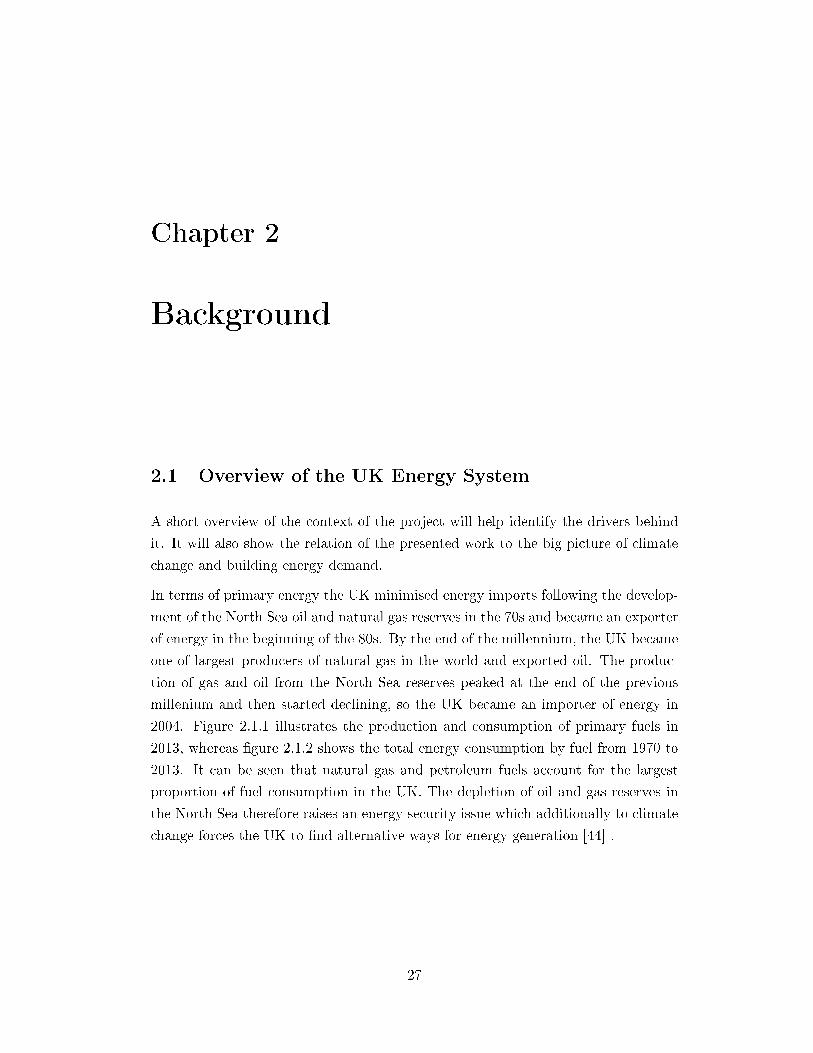
2004. Figure 2.1.1 illustrates the production and consumption of primary fuels in
2013, whereas �gure 2.1.2 shows the total energy consumption by fuel from 1970 to
2013. It can be seen that natural gas and petroleum fuels account for the largest
proportion of fuel consumption in the UK. The depletion of oil and gas reserves in
the North Sea therefore raises an energy security issue which additionally to climate
change forces the UK to �nd alternative ways for energy generation [44] .
27
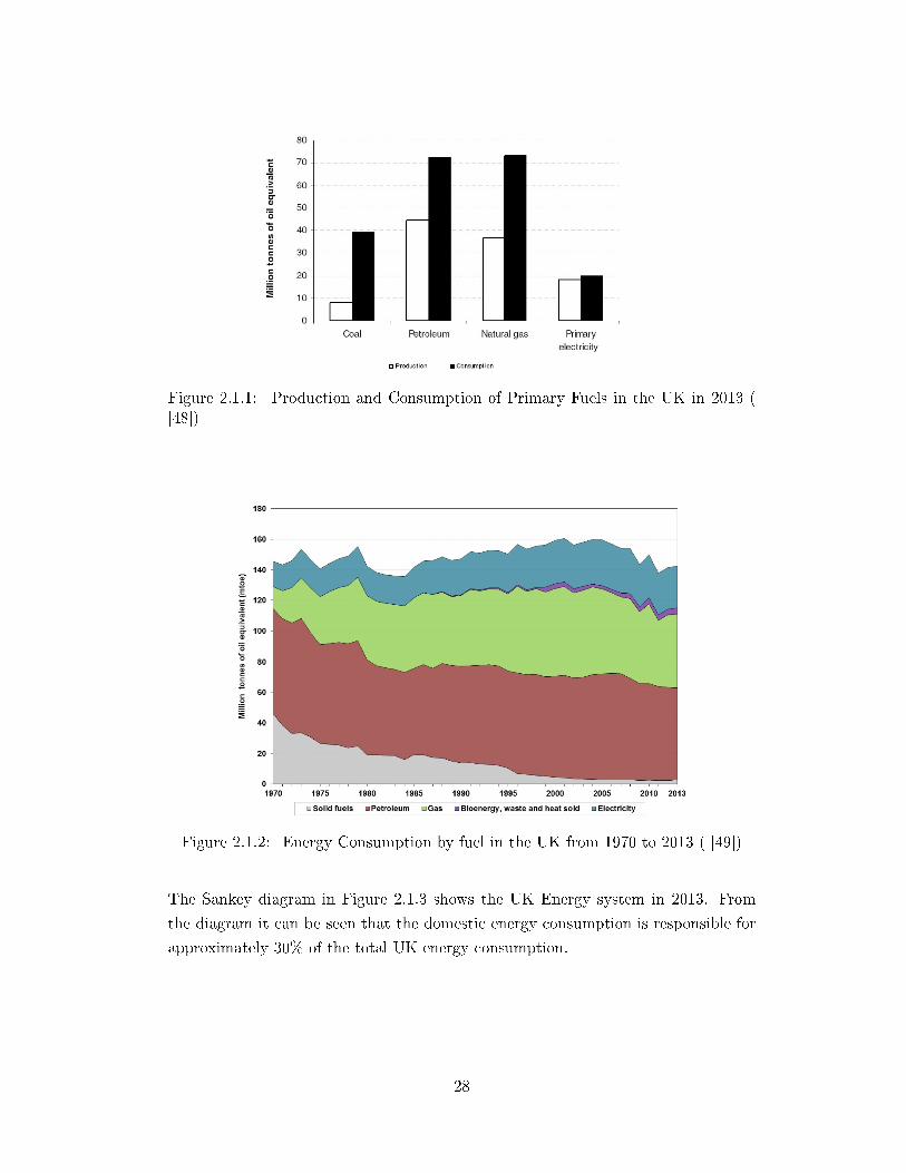
Figure 2.1.1: Production and Consumption of Primary Fuels in the UK in 2013 ([48])
Figure 2.1.2: Energy Consumption by fuel in the UK from 1970 to 2013 ( [49])
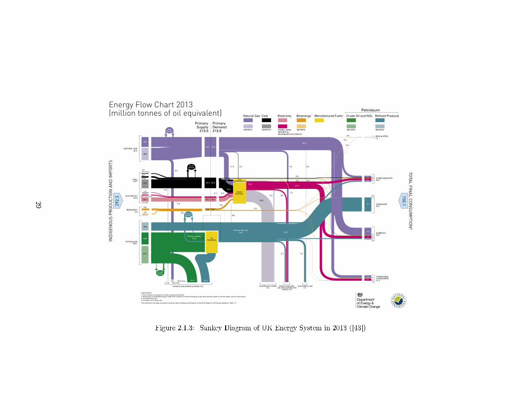
The Sankey diagram in Figure 2.1.3 shows the UK Energy system in 2013. From
the diagram it can be seen that the domestic energy consumption is responsible for
approximately 30% of the total UK energy consumption.
28
GasStocks
CoalStocks
ProductStocks
CrudeStocks
36.5
46.0
5.5
32.7
NATURAL GAS82.5
COAL40.7
ELECTRICITY20.0
OTHER
IMPORTS
2.2
3.0 HYDRO & WIND
15.4
PETROLEUM140.1
NUCLEAR
30.9
44.5
64.7
73.2 73.2
9.4
0.5
17.4 5.4 0.5
0.1
48.4
27.3
2.2
2.0
1.2
44.0
31.9
2.0
PrimarySupply
213.5
PrimaryDemand213.9
4.64.0
0.6
0.20.1
67.3
7.04.7
31.437.0Coal
Gas
OILREFINERIES
POWERSTATIONS
OTHERTRANSFORMATION
19.7
39.4
32.4
39.3
19.719.7
CONVERSION LOSSES48.1
ENERGY INDUSTRYUSE AND DISTRIBUTION
LOSSES 15.8
NON-ENERGY USE7.6
EXPORTS AND MARINE BUNKERS 78.9
Primary demand72.8
IRON & STEEL1.3
OTHER INDUSTRY22.9
TRANSPORT53.4
DOMESTIC43.8
7.6
4.3
1.40.9
52.0
0.4
29.6
0.5
2.8 0.3
0.9
10.3
1.2
OTHER FINAL CONSUMERS 21.0
0.5
0.5
Primary supply72.5
5.6
FOOTNOTES:1. Coal imports and exports include manufactured fuels.
3. Includes heat sold.2. Bioenergy is renewable energy made from material of recent biological origin derived from plant or animal matter, known as biomass.
4. Includes non-energy use.
This flowchart has been produced using the style of balance and figures in the 2014 Digest of UK Energy Statistics, Table 1.1.
0.3
2.5DEEP MINED
0.4
Electricity
0.3
BIOENERGY9.0
IMPORTS
1.5
6.98.88.8
0.2
Bioenergy
0.6
1.1
0.3
2.9
5.8
Natural Gas
IMPORTS
Coal
IMPORTS1
Electricity
HYDRO, WIND, IMPORTS & SECONDARY ELECTRICITY
Manufactured Fuels3 Crude Oil and NGL
IMPORTS
Refined Products
IMPORTS
Petroleum
IMPORTS
Bioenergy 2
Energy Flow Chart 2013 (million tonnes of oil equivalent)
IND
IGEN
OU
S P
RO
DU
CTI
ON
AN
D IM
PO
RTS
292.
3TO
TAL FINA
L CO
NSU
MP
TION
4
150.1
8.1
9.8
8.7
Figure 2.1.3: Sankey Diagram of UK Energy System in 2013 ([43])
29

UK energy policy concentrates on energy security as the country is now importing
the majority of its energy. The priorities of the energy policy are to achieve the EU
target of 20% reduction of the UK's energy consumption by 2020. This EU target
is described in the European Commission's Emissions Trading System (EU ETS)
and was �rst introduced by Directive 2003/87/EC [61]. The UK has also introduced
a more optimistic target which has been implemented into the legislation as the
Climate Change Act 2008 and is an 80% reduction in CO2 emissions from 1990
levels by 2050 [82] . This will be achieved by implementing the measures de�ned
within the EU Energy E�ciency Action Plan in the following sectors: transport,
improved e�ciency of equipment, changing citizens' energy behaviour, technology
and energy savings in buildings [59].
2.2 Household Energy Demand
Household energy consumption was around a third of the �nal energy consumption
in the UK in 2010. This is an increase of approximately 30% and 20% compared
to the 1970 and 1990 levels respectively. Some of this increase has been caused
by the additional UK households constructed in this period and the increase in
the population since 1990. The main fuel in dwellings has also drastically changed
since the 70s when the primary fuel was coal, followed by natural gas; In 2010 coal
represented only 1% of the total household energy consumption whereas natural gas
covered the majority (69%) [49]. The fuel mix of residential buildings since 1970 is
represented in Figure 2.2.1.
30
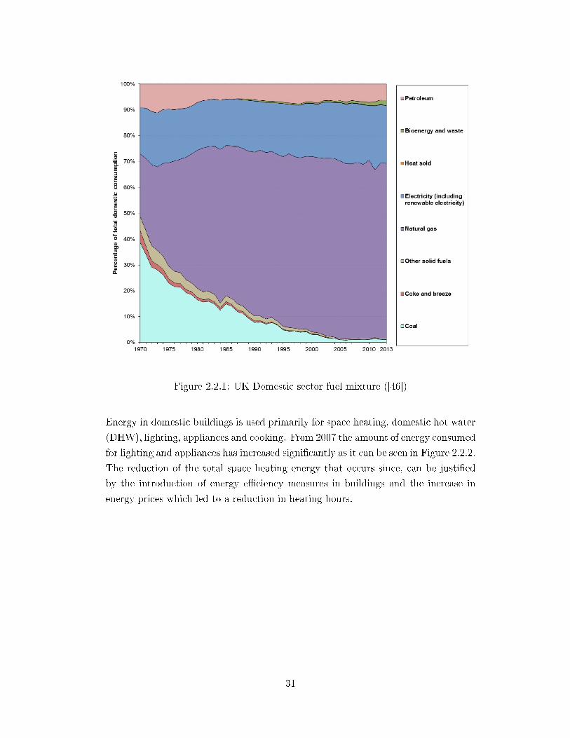
Figure 2.2.1: UK Domestic sector fuel mixture ([46])
Energy in domestic buildings is used primarily for space heating, domestic hot water
(DHW), lighting, appliances and cooking. From 2007 the amount of energy consumed
for lighting and appliances has increased signi�cantly as it can be seen in Figure 2.2.2.
The reduction of the total space heating energy that occurs since, can be justi�ed
by the introduction of energy e�ciency measures in buildings and the increase in
energy prices which led to a reduction in heating hours.
31
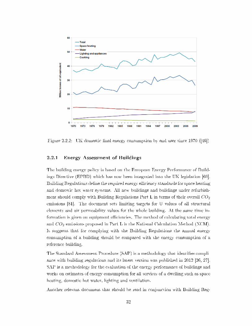
Figure 2.2.2: UK domestic �nal energy consumption by end user since 1970 ([46])
2.2.1 Energy Assessment of Buildings
The building energy policy is based on the European Energy Performance of Build-
ings Directive (EPBD) which has now been integrated into the UK legislation [60].
Building Regulations de�ne the required energy e�ciency standards for space heating
and domestic hot water systems. All new buildings and buildings under refurbish-
ment should comply with Building Regulations Part L in terms of their overall CO2
emissions [81]. The document sets limiting targets for U values of all structural
elements and air permeability values for the whole building. At the same time in-
formation is given on equipment e�ciencies. The method of calculating total energy
and CO2 emissions proposed in Part L is the National Calculation Method (NCM).
It suggests that for complying with the Building Regulations the annual energy
consumption of a building should be compared with the energy consumption of a
reference building.
The Standard Assessment Procedure (SAP) is a methodology that identi�es compli-
ance with building regulations and its latest version was published in 2012 [26, 27].
SAP is a methodology for the evaluation of the energy performance of buildings and
works on estimates of energy consumption for all services of a dwelling such as space
heating, domestic hot water, lighting and ventilation.
Another relevant document that should be read in conjunction with Building Reg-
32
ulations Part L is the Domestic Heating Compliance Guide (DHCG). The DHCG
provides information on the various equipment that can be used in household heating
and DHW, together with information on limiting seasonal e�ciencies [83].
2.3 Domestic Micro-CHP
Micro-generation refers to systems suitable to generate energy at a small scale for
use in domestic or small commercial properties. EU's Co-generation directive de�nes
micro-generation as any system that generates electricity below 50 kWe [62]. In the
UK however micro-generation is limited to 3 kW electrical and 20 kW thermal output
[72]. Micro-generation can be broadly categorised in the following:
1. Micro-CHP technologies
2. Photovoltaics, solar thermal and wind turbines
3. Heating using biomass boilers or heat pumps.
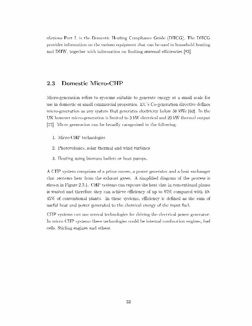
A CHP system comprises of a prime mover, a power generator and a heat exchanger
that recovers heat from the exhaust gases. A simpli�ed diagram of the process is
shown in Figure 2.3.1. CHP systems can capture the heat that in conventional plants
is wasted and therefore they can achieve e�ciency of up to 85% compared with 40-
45% of conventional plants. In these systems, e�ciency is de�ned as the sum of
useful heat and power generated to the chemical energy of the input fuel.
CHP systems can use several technologies for driving the electrical power generator.
In micro-CHP systems these technologies could be internal combustion engines, fuel
cells, Stirling engines and others.
33
Fuel Input Prime Mover Generator Electricity
Waste Heat
Exh
aust
gas
es
Heat Recovery
Waste heat
Heat
Figure 2.3.1: Simpli�ed diagram of a CHP system showing energy �ows
2.4 Fuel Cell Technology
2.4.1 Overview of Fuel Cell Technologies
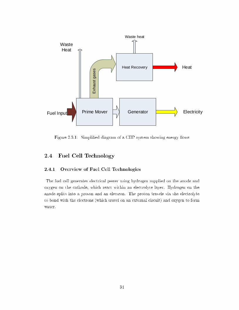
The fuel cell generates electrical power using hydrogen supplied on the anode and
oxygen on the cathode, which react within an electrolyte layer. Hydrogen on the
anode splits into a proton and an electron. The proton travels via the electrolyte
to bond with the electrons (which travel on an external circuit) and oxygen to form
water.
34
Figure 2.4.1: Fuel Cell Basic Operation ( [65])
The overall fuel cell reaction is:
2H2 +O2 → 2H2O (2.4.1)
There are di�erent types of fuel cells categorised by their electrolyte. The most
important are:
� Phosphoric Acid Fuels Cells (PAFC)
� Molten Carbonate Fuel Cells (MCFC)
� Proton Exchange Membrane Fuel Cell (PEMFC)
� Solid Oxide Fuel Cells (SOFC)
� Alkaline Fuel Cells (AFC) .
A comparison between the di�erent types of fuel cells can be seen in the next table:
35

Table 2.1: Comparison of Fuel Cell Technologies ([122])PEMFC PAFC MCFC SOFC
Charge H+ions H+ions CO=3 ions O=ions
Carrier
Polymeric Phosphoric Phosphoric Solid ceramic,
membrane acid acid Yttria stabilised
Electrolyte solutions (immobilised zirconia
liquid)
Construction Plastic, metal Carbon, High Ceramic,
or Carbon porous temperature high
ceramics metals, temperature
porous metals
ceramic
Oxidant Air Air or Air Air
or O2 or O2enriched air
Fuel
Hydrocarbons Hydrocarbons Hydrogen, Natural gas
or or natural gas, or
methanol alcohols propane propane
Temperature 65-85 oC 150-200 oC 600-700 oC 700-1000 oC
Electrical 25-35 % 35-45 % 40-50 % 45-55 %
E�ciency
Contaminants CO, sulfur CO, sulfur sulfur sulfur
SOFC and PEMFC have received more attention than the other types and there are
many commercially available products for various stationary or mobile applications
[10, 51, 122] .
2.4.2 Fuel Cell Operation
The open circuit voltage (OCV) of a fuel cell is given by the following equation:
Eocv =−Δg2F
(2.4.2)
where ∆g is the Gibbs free energy and F the Faraday constant. This represents a
�no losses� voltage and in practise is never achieved due to three main losses:
Activation Losses
Activation losses are related to the speed of the reactions on the surface of the
electrodes that move the electrons to or from the anode. These losses can be
36
calculated using the Tafel equation:
ΔVact =RT
2aFln
(i
io
)(2.4.3)
where a is a constant called the charge transfer coe�cient. Its value depends
on the reaction and the material of the electrode. For the hydrogen electrode,
its value is about 0.5. For the oxygen electrode the charge transfer coe�cient is
between 0.1 and 0.5. iο is called the exchange current density and is responsible
for the control of the performance of the electrode. T is the temperature, R is
the gas constant and i is the current density [89].
Ohmic Losses
This voltage drop is caused by the resistance to the �ow of electrons through
the material of the electrodes and is proportional to current density. The ohmic
losses are given by equation (2.4.4)
∆Vohm = ir (2.4.4)
where r is the area-speci�c resistance.
Mass Transport or Concentration Losses
These result from the change in concentration of the reactants at the surface
of the electrodes as the fuel is used. The voltage drop due to concentration
losses is given by equation 2.4.5.
∆Vcon = −RT2F
ln
(1− i
i1
)(2.4.5)
Overall the voltage is given by subtracting all the losses from the OCV:
V = Eocv −∆Vact −ΔVohm −ΔVcon (2.4.6)
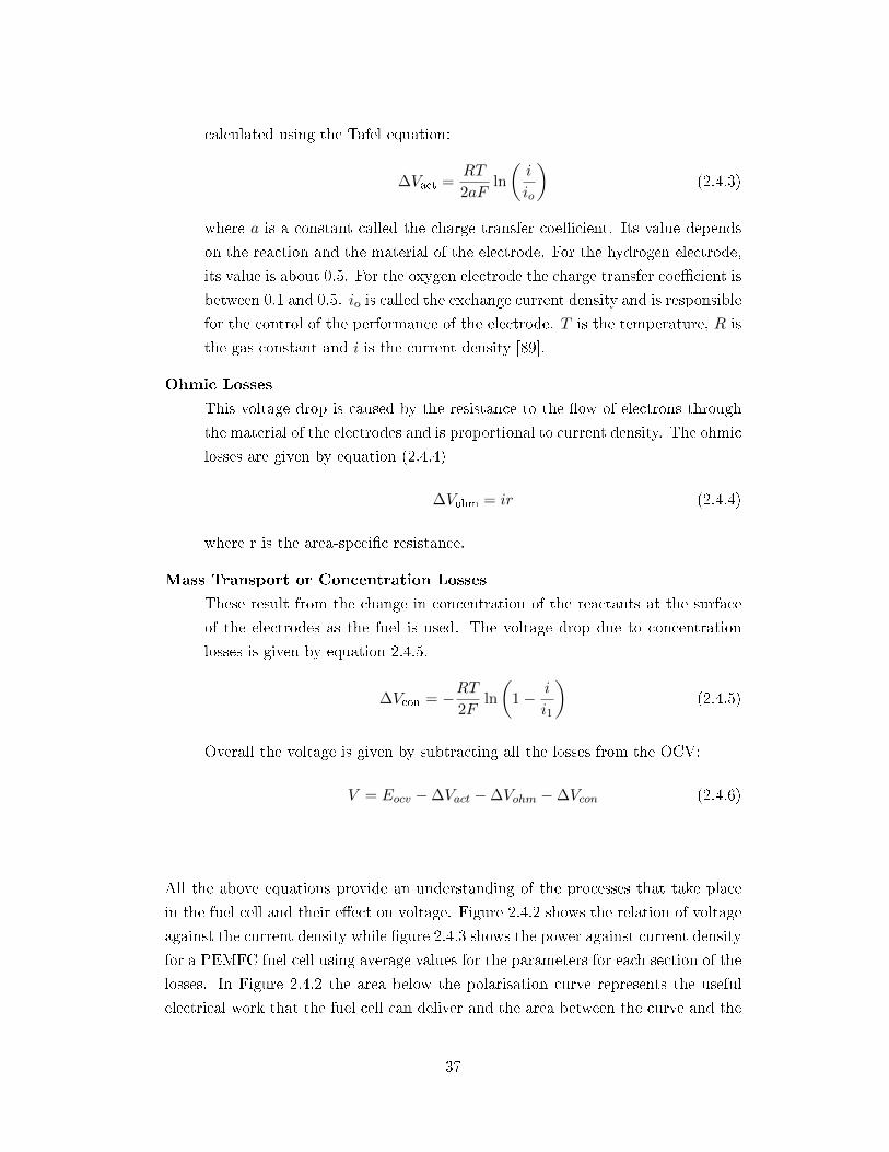
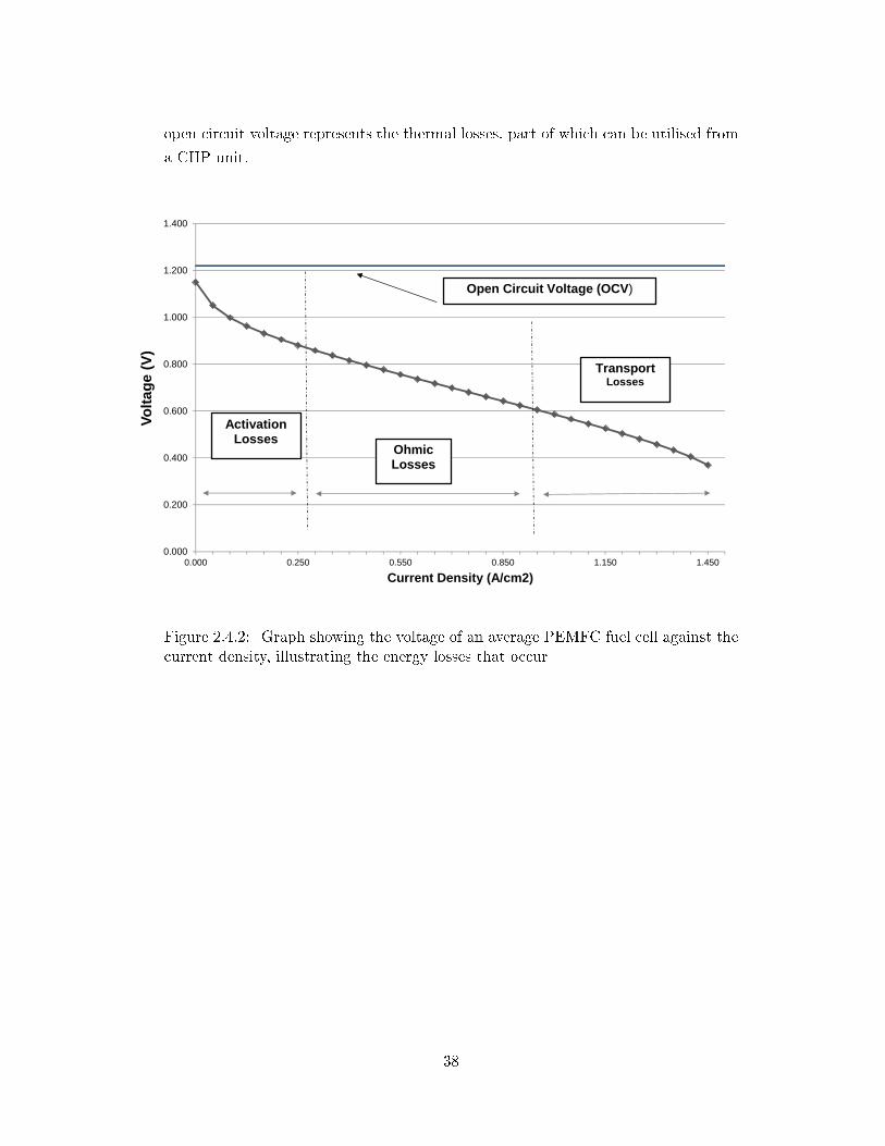
All the above equations provide an understanding of the processes that take place
in the fuel cell and their e�ect on voltage. Figure 2.4.2 shows the relation of voltage
against the current density while �gure 2.4.3 shows the power against current density
for a PEMFC fuel cell using average values for the parameters for each section of the
losses. In Figure 2.4.2 the area below the polarisation curve represents the useful
electrical work that the fuel cell can deliver and the area between the curve and the
37
open circuit voltage represents the thermal losses, part of which can be utilised from
a CHP unit.
0.000
0.200
0.400
0.600
0.800
1.000
1.200
1.400
0.000 0.250 0.550 0.850 1.150 1.450
Volt
age
(V)
Current Density (A/cm2)
Open Circuit Voltage (OCV)
ActivationLosses
Ohmic Losses
TransportLosses
Figure 2.4.2: Graph showing the voltage of an average PEMFC fuel cell against thecurrent density, illustrating the energy losses that occur
38
0.000
0.100
0.200
0.300
0.400
0.500
0.600
0.700
0.000 0.250 0.550 0.850 1.150 1.450
Po
wer
(kW
)
Current Density (A/cm2)
Figure 2.4.3: Graph showing the power output of an average PEMFC fuel cellagainst the current density
2.4.3 Fuel Cell E�ciency
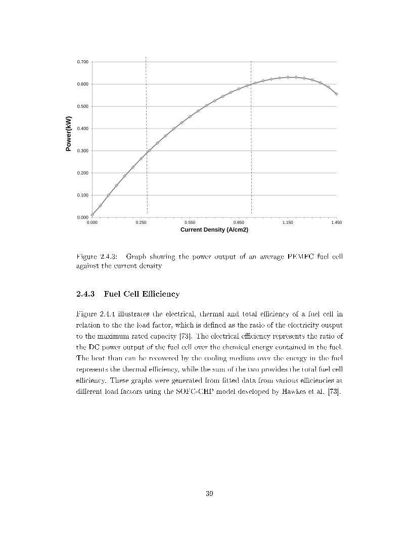
Figure 2.4.4 illustrates the electrical, thermal and total e�ciency of a fuel cell in
relation to the the load factor, which is de�ned as the ratio of the electricity output
to the maximum rated capacity [73]. The electrical e�ciency represents the ratio of
the DC power output of the fuel cell over the chemical energy contained in the fuel.
The heat than can be recovered by the cooling medium over the energy in the fuel
represents the thermal e�ciency, while the sum of the two provides the total fuel cell
e�ciency. These graphs were generated from �tted data from various e�ciencies at
di�erent load factors using the SOFC-CHP model developed by Hawkes et al. [73].
39
0
10
20
30
40
50
60
70
80
90
100
0 0.1 0.2 0.3 0.4 0.5 0.6 0.7 0.8 0.9 1
Eff
icie
ncy
(%
)
Load Factor
Electrical Efficiency Total Efficiency Thermal Efficiency
Figure 2.4.4: Graph showing the electrical, thermal and total e�ciency of an SOFCin relation to the load factor [73]
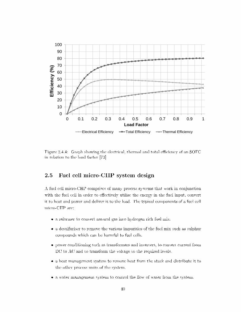
2.5 Fuel cell micro-CHP system design
A fuel cell micro-CHP comprises of many process systems that work in conjunction
with the fuel cell in order to e�ectively utilise the energy in the fuel input, convert
it to heat and power and deliver it to the load. The typical components of a fuel cell
micro-CHP are:
� a reformer to convert natural gas into hydrogen rich fuel mix.
� a desulfuriser to remove the various impurities of the fuel mix such as sulphur
compounds which can be harmful to fuel cells.
� power conditioning such as transformers and inverters, to convert current from
DC to AC and to transform the voltage to the required levels.
� a heat management system to remove heat from the stack and distribute it to
the other process units of the system.
� a water management system to control the �ow of water from the system.
40

� a control system to regulate fuel input, power output and operation.
An example of a fuel cell micro-CHP with all the components and interconnections
is shown in Figure 2.5.1.
Figure 2.5.1: Schematic Diagram of fuel cell micro-CHP components ([125])
2.5.1 Fuel Processing
Hydrogen does not exist in nature as a fuel, therefore the use of carbon-based fuels
such as natural gas is necessary. This requires the use of a reformer which provides a
supply of hydrogen rich gas from the fuel source. The operating temperature of the
fuel cell determines whether the reformer is internal or external. For the reformer to
be internal, the operating temperature of the stack must be high. SOFCs operate at
a high temperature and therefore reform internally avoiding the need of additional
subsystems external to the fuel cell stack. However, a pre-reformer is sometimes used
in medium temperature SOFCs.
The two main methods of reforming are endothermic steam reforming (SR) and
exothermic partial oxidation reaction (POX). In the case of steam reforming, the fuel
is combined with steam to produce CO and H2 by vaporisation at high temperature.
The methane steam reforming reaction is shown below:
41
CH4 +H2O → CO + 3H2 (2.5.1)
[ΔH = 206 kJ mol−1]
In the exothermic partial oxidation reaction, hydrocarbons and oxygen combine to
form CO and H2.The methane partial oxidation reaction is shown below:
CH4 +1
2O2 → CO + 2H2 (2.5.2)
[ΔH = =247 kJ mol−1]
The subsequent CO generated by either process is converted into CO2 with the
addition of water in a water-gas shift reaction. The gas shift reaction is shown
below:
CO +H2O → CO2 +H2 (2.5.3)
[ΔH = -41 kJ mol−1]
Natural gas reforming is endothermic, so heat needs to be supplied to the reformer
at high temperature for a reasonable conversion rate to be achieved.
2.5.2 Electricity Conditioning
The fuel cell produces DC electricity which must be converted to AC. The use of
inverters is therefore necessary. Transformers are also used to obtain the required
voltage. In domestic systems, the electricity is converted to a single phase AC voltage.
In addition, current, voltage and frequency are controlled to ensure the quality of
electricity is maintained [89, 103, 128].
2.5.3 Heat Management
In order to use heat within the fuel cell micro-CHP, a management system is required
that can capture and exchange heat through heat exchangers. Heat utilisation and
management in fuel cell micro-CHP is discussed in detail in Chapter 4.
42
2.5.4 Controls
Fuel cells micro-CHPs are complex systems, so in order to perform well, a control
system must be in place. The fact that so many process units operate together as
one system makes the control of a micro-CHP a complicated task. A control system
includes valves, actuators and control units. SOFC fuel cells have long start up
times mainly due to their high operating temperature. Degradation of fuel cell's
performance over time can a�ect the projected lifetime of a micro-CHP system and
a�ect the investment in the technology. An appropriate control strategy can minimise
the e�ects of stack degradation [88, 92, 118, 129, 131].
2.6 Fuel cell micro-CHP Products
In terms of product availability, there are many manufacturers that produce fuel cell
units for various applications and sizes, and a number of them produce packaged fuel
cell micro-CHP units that can be installed in domestic properties. Companies such
as Ceramic Fuel Cells, BG MicroGen, EcoPower, WhispeGen, Sulzer Hexis and Baxi
are producing micro-CHP systems of various technologies and capacities. Japan and
generally Asia is a developed fuel cell market with strong government support. The
global sales market share for the Asian region exceeds 60% and reaches $1.5 billion
[66, 120]. Japan is active on production of fuel cell products with Kyocera, TOTO
and Nippon Oil developing micro-CHP systems around the 1 kWe capacity group
[51].
Ceramic Fuel Cells has developed a fuel cell micro-CHP product named BlueGen. It
is based on a solid oxide fuel cell system with a heat to power ratio of 0.5 kWth to
1 kWe, aiming to achieve a high electrical e�ciency. An image of the BlueGen unit
is shown in Figure 2.6.1a [34].
Sulzer Hexis produces the Galileo 1000N system which is based on a SOFC and
generates 1 kW of electrical power and 2 kW of heat [113]. The unit includes an
integrated 20 kW gas �red condensing boiler which can be used to cover heating and
DHW when the fuel cell thermal output is not su�cient. An image of the unit is
shown in Figure 2.6.1b.
43
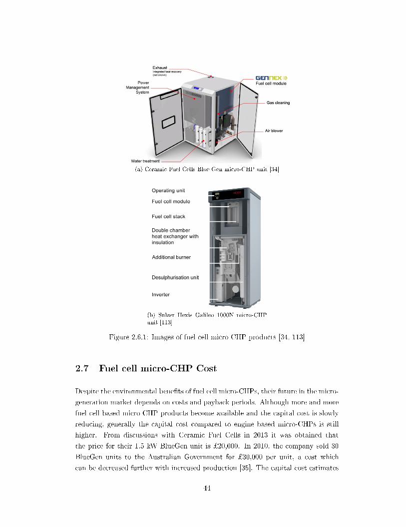
(a) Ceramic Fuel Cells Blue Gen micro-CHP unit [34]
(b) Sulzer Hexis Galileo 1000N micro-CHPunit [113]
Figure 2.6.1: Images of fuel cell micro-CHP products [34, 113]
2.7 Fuel cell micro-CHP Cost
Despite the environmental bene�ts of fuel cell micro-CHPs, their future in the micro-
generation market depends on costs and payback periods. Although more and more
fuel cell based micro-CHP products become available and the capital cost is slowly
reducing, generally the capital cost compared to engine based micro-CHPs is still
higher. From discussions with Ceramic Fuel Cells in 2013 it was obtained that
the price for their 1.5 kW BlueGen unit is ¿20,000. In 2010, the company sold 30
BlueGen units to the Australian Government for ¿30,000 per unit, a cost which
can be decreased further with increased production [35]. The capital cost estimates
44
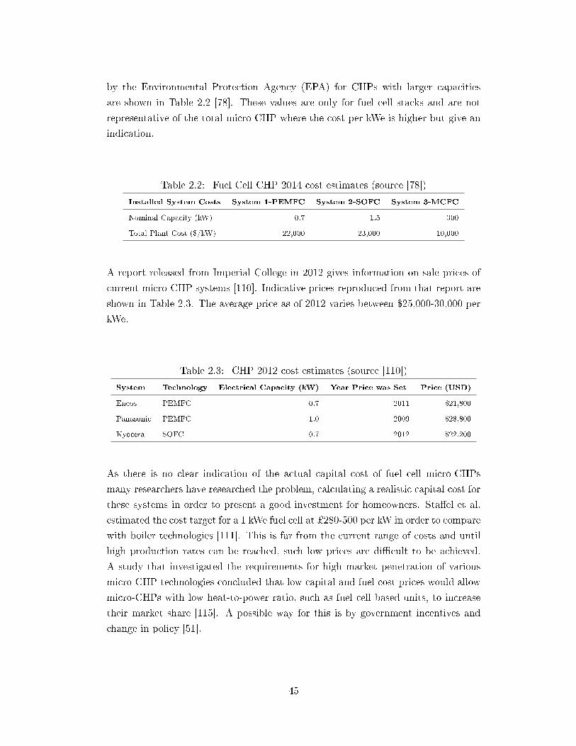
by the Environmental Protection Agency (EPA) for CHPs with larger capacities
are shown in Table 2.2 [78]. These values are only for fuel cell stacks and are not
representative of the total micro-CHP where the cost per kWe is higher but give an
indication.
Table 2.2: Fuel Cell CHP 2014 cost estimates (source [78])
Installed System Costs System 1-PEMFC System 2-SOFC System 3-MCFC
Nominal Capacity (kW) 0.7 1.5 300
Total Plant Cost ($/kW) 22,000 23,000 10,000
A report released from Imperial College in 2012 gives information on sale prices of
current micro-CHP systems [110]. Indicative prices reproduced from that report are
shown in Table 2.3. The average price as of 2012 varies between $25,000-30,000 per
kWe.
Table 2.3: CHP 2012 cost estimates (source [110])
System Technology Electrical Capacity (kW) Year Price was Set Price (USD)
Eneos PEMFC 0.7 2011 $21,800
Panasonic PEMFC 1.0 2009 $28,800
Kyocera SOFC 0.7 2012 $22,200
As there is no clear indication of the actual capital cost of fuel cell micro-CHPs
many researchers have researched the problem, calculating a realistic capital cost for
these systems in order to present a good investment for homeowners. Sta�el et al.
estimated the cost target for a 1 kWe fuel cell at ¿280-500 per kW in order to compare
with boiler technologies [111]. This is far from the current range of costs and until
high production rates can be reached, such low prices are di�cult to be achieved.
A study that investigated the requirements for high market penetration of various
micro-CHP technologies concluded that low capital and fuel cost prices would allow
micro-CHPs with low heat-to-power ratio, such as fuel cell based units, to increase
their market share [115]. A possible way for this is by government incentives and
change in policy [51].
45
2.8 Policy and Field Trials
The policy with regard to micro-generation is outlined in the �Micro-generation
Strategy� of the Department of Energy and Climate Change (DECC) in 2011 [47].
The purpose of the document is to attract investments in micro-generation by intro-
ducing support schemes such as the Feed-in-Tari� (FIT) and the Renewable Heat
Incentive (RHI) which reward �nancially every kWh of energy generated from re-
newables or micro-CHPs. Technologies such as fuel cells are also featured in the
document. The document concludes that the most suitable buildings for such tech-
nology have to be determined. At the same time micro-CHP systems have to be
established as �exible enough systems to satisfy the variable heat loads of buildings.
Heat storage is also mentioned in the document and is considered a method that
combined with CHP units can reduce CO2 emissions.
Carbon Trust's report titled �Micro CHP Accelerator� demonstrates the bene�ts of
micro-CHP �eld trials [32]. The programme included the installation of 87 micro-
CHP units based on internal combustion and Stirling engines in domestic and com-
mercial applications in the UK. The report presents the energy and cost savings in
the �eld trials and concludes that the economics of micro-CHP systems can be im-
proved further by increasing the electrical e�ciency of the systems. According to the
report the micro-CHP - household system would perform better if the electrical e�-
ciency of the prime mover was higher and the electricity production similar to heat
production. In addition, the report claims that with optimised controls, the car-
bon savings by domestic micro-CHP systems could potentially be higher. The trials
did not include any fuel cell micro-CHPs as the commercially available products at
the period the project started were limited. However, based on the heat-to-power
characteristics and higher electrical e�ciency, fuel cell based micro-CHPs may be
more e�ective over other micro-CHP technologies which are based on thermal en-
gines in terms of the potential to reduce energy consumption in buildings. Despite
the bene�cial technical characteristics of fuel cells, there has been small interest by
manufacturers in developing fuel cell micro-CHPs compared to engine based tech-
nologies. The Energy Saving Trust places the fuel cell micro-CHP as an emerging
technology in the energy market and suggests that this is due to the reason that the
cost per kW of fuel cell is still much greater compared to established technologies
such as the Stirling or internal combustion engines [56].
Ene.�eld [54] is a fuel cell micro-CHP trial programme that runs in 11 countries in
Europe and aims to install up to 1,000 systems. The programme is supported by
several European micro-CHP manufacturers and the data will be used to in�uence
46
policy support by demonstrating the cost and environmental bene�ts of the techno-
logy. However the reports [55] available on the programme's website do not present
any results from the �eld trials suggesting that performance data of installed fuel
cell micro-CHPs are not yet available.
Ceramic Fuel Cells together with Crest Nicholson, a UK contractor, has installed
a BlueGen 1.5 kWe unit in a four-bedroom family home in Epsom, Surrey. The
building that the fuel cell micro-CHP unit is installed in, is a high insulation home
with very low space heating demand. The BlueGen can then provide all the heat
demand of the house without a need for an auxiliary boiler [40]. Following the
installation there are no subsequent reports from the contractor or the manufacturer
on the environmental or cost bene�ts of this installation. This is to add to the overall
lack of data from the �eld with regard to fuel cell micro-CHP installations.
2.9 Thermal Comfort and Heating Systems
Buildings require heating to maintain comfortable conditions for the occupants.
Thermal comfort varies between di�erent people depending on their health, age,
metabolic rate, clothing and other environmental factors such as temperature and
humidity. Engineers that design heating systems work on a common reference when
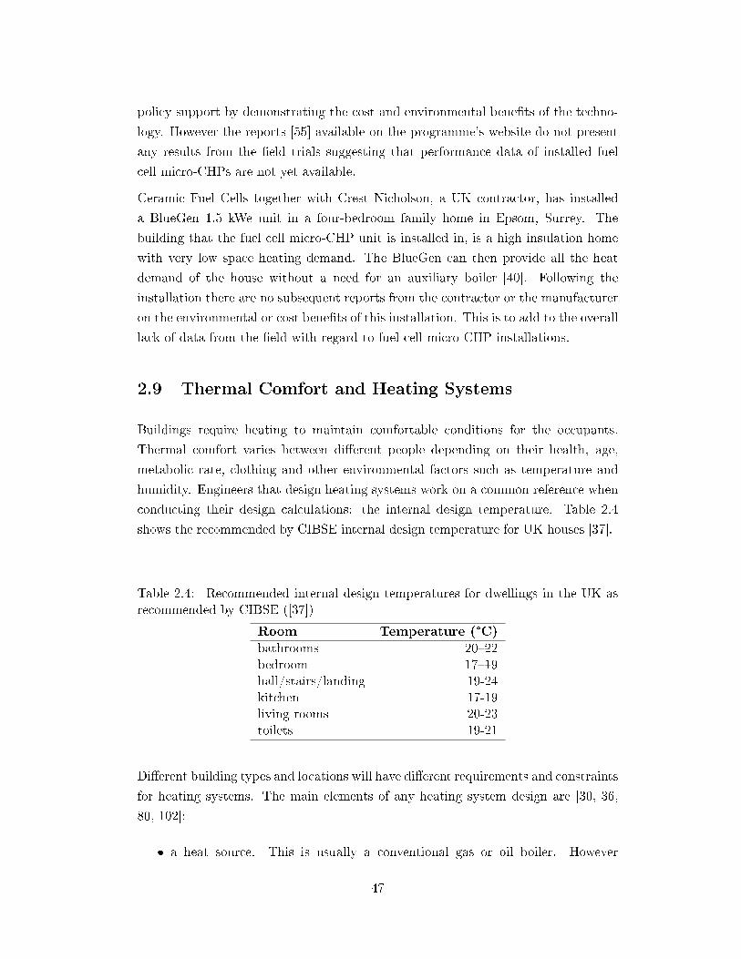
conducting their design calculations: the internal design temperature. Table 2.4
shows the recommended by CIBSE internal design temperature for UK houses [37].
Table 2.4: Recommended internal design temperatures for dwellings in the UK asrecommended by CIBSE ([37])
Room Temperature (°C)
bathrooms 20�22bedroom 17�19hall/stairs/landing 19-24kitchen 17-19living rooms 20-23toilets 19-21
Di�erent building types and locations will have di�erent requirements and constraints
for heating systems. The main elements of any heating system design are [30, 36,
80, 102]:
� a heat source. This is usually a conventional gas or oil boiler. However
47
other sources of heat could be heat pumps [109], micro-CHP systems and solar
thermal panels.
� a heat distribution system. Heat could be delivered using water or air. A pipe
or a duct network is commonly used. In the case of a pipe network, this is
called a Low Temperature Hot Water (LTHW) pipe network and uses water
at temperatures in the range of 30-90 °C.
� a heat emitter. The radiator is the most popular heat emitter in UK houses. A
temperature di�erence (ΔT) of around 10 °C which sometimes can be extended
to 20 °C is maintained between the water temperature in the supply and re-
turn pipework. Under�oor heating despite being a more costly system is more
e�cient than radiators because of the lower operating temperature (30-50 °C).
Figure 2.9.1 shows a radiator and an under�oor heating system. Figure 2.9.3
shows a common system design used in dwellings with a separate hot water
tank.
� a control system that ensures that the heat source is operated at the correct
output level. This usually requires a central controller with space temperature
reading via a thermostat and in some cases secondary control on the heat
emitters such as thermostatic radiator valves (TRV).
48
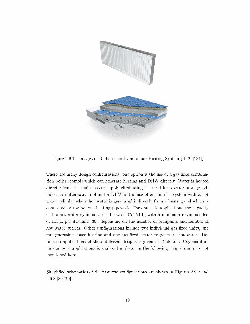
Figure 2.9.1: Images of Radiator and Under�oor Heating System ([112],[124])
There are many design con�gurations: one option is the use of a gas �red combina-
tion boiler (combi) which can generate heating and DHW directly. Water is heated
directly from the mains water supply eliminating the need for a water storage cyl-
inder. An alternative option for DHW is the use of an indirect system with a hot
water cylinder where hot water is generated indirectly from a heating coil which is
connected to the boiler's heating pipework. For domestic applications the capacity
of the hot water cylinder varies between 75-250 L, with a minimum recommended
of 115 L per dwelling [30], depending on the number of occupants and number of
hot water outlets. Other con�gurations include two individual gas �red units, one
for generating space heating and one gas �red heater to generate hot water. De-
tails on applications of these di�erent designs is given in Table 2.5. Cogeneration
for domestic applications is analysed in detail in the following chapters so it is not
mentioned here.
Simpli�ed schematics of the �rst two con�gurations are shown in Figures 2.9.2 and
2.9.3 [39, 79].
49
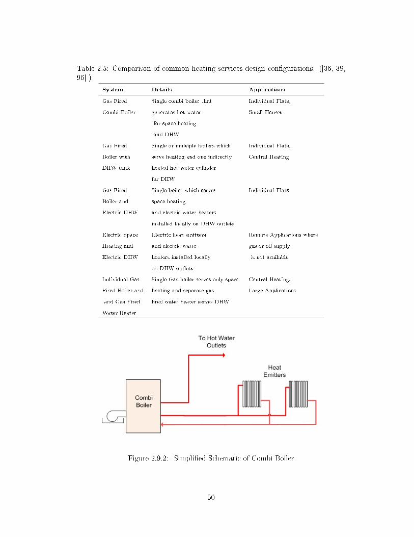
Table 2.5: Comparison of common heating services design con�gurations. ([36, 38,96] )
System Details Applications
Gas Fired Single combi boiler that Individual Flats,
Combi Boiler generates hot water Small Houses
for space heating
and DHW
Gas Fired Single or multiple boilers which Individual Flats,
Boiler with serve heating and one indirectly Central Heating
DHW tank heated hot water cylinder
for DHW
Gas Fired Single boiler which serves Individual Flats
Boiler and space heating
Electric DHW and electric water heaters
installed locally on DHW outlets
Electric Space Electric heat emitters Remote Applications where
Heating and and electric water gas or oil supply
Electric DHW heaters installed locally is not available
on DHW outlets
Individual Gas Single Gas boiler serves only space Central Heating,
Fired Boiler and heating and separate gas Large Applications
and Gas Fired �red water heater serves DHW
Water Heater
Figure 2.9.2: Simpli�ed Schematic of Combi Boiler
50
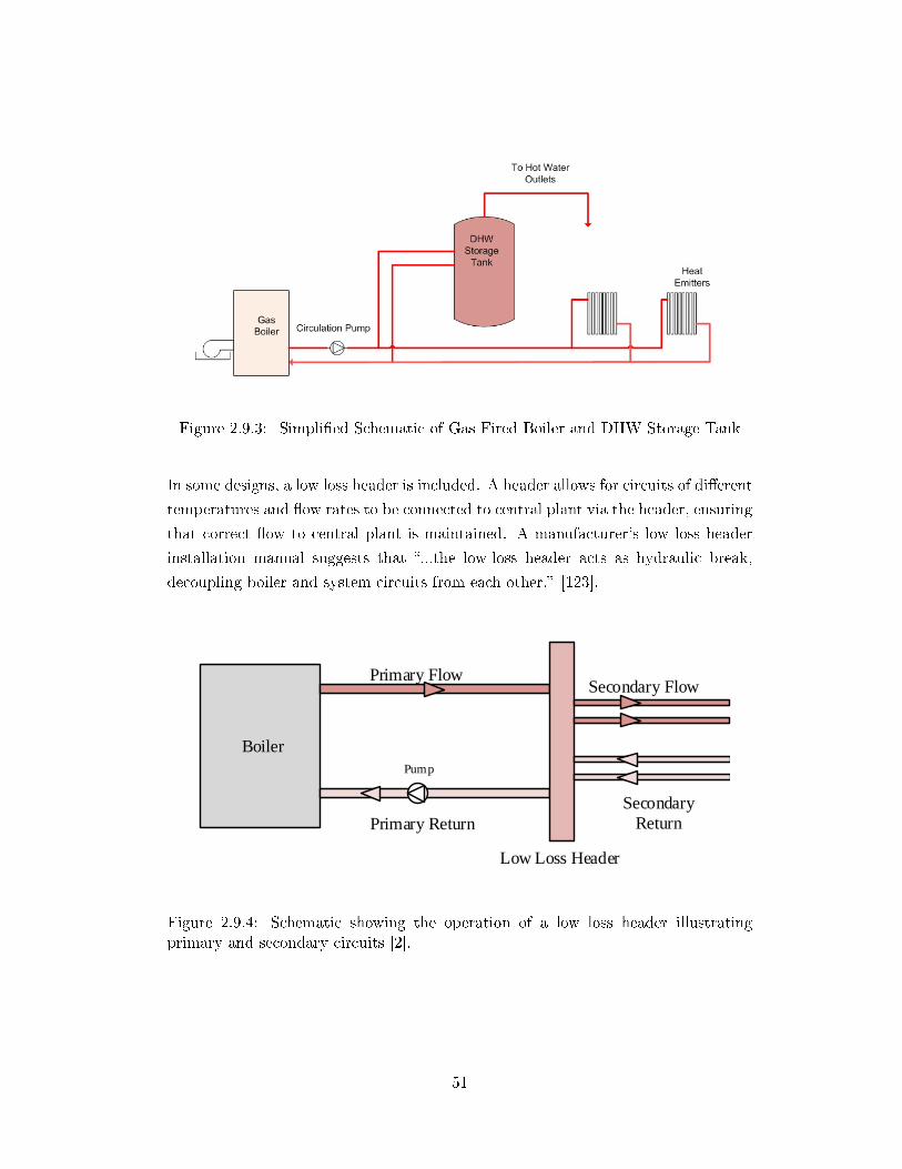
Figure 2.9.3: Simpli�ed Schematic of Gas Fired Boiler and DHW Storage Tank
In some designs, a low loss header is included. A header allows for circuits of di�erent
temperatures and �ow rates to be connected to central plant via the header, ensuring
that correct �ow to central plant is maintained. A manufacturer's low loss header
installation manual suggests that �...the low-loss header acts as hydraulic break,
decoupling boiler and system circuits from each other.� [123].
�
Low Loss Header
BoilerPump
Primary Flow
Primary Return
Secondary Flow
Secondary Return
Figure 2.9.4: Schematic showing the operation of a low loss header illustratingprimary and secondary circuits [2].
51
Chapter 3
Previous Work
3.1 Modelling Fuel Cell micro-CHPs for domestic applic-
ations
As �eld data have been limited, many researchers have developed models to predict
the performance of fuel cell micro-CHPs in dwellings [13, 15, 16, 21, 52, 70]. The
use of models to examine various scenarios is natural as fuel cell micro-CHPs are
an emerging and not an established technology. However, the potential bene�ts
of fuel cells and the increasing number of available products increase interest in
modelling fuel cells for micro-generation [9]. Usually researchers estimate energy
savings or cost reduction from the use of fuel cell systems. Some researchers use
simulation methods to evaluate di�erent scenarios: simulation can identify values
for a speci�c characteristic of the system under examination over a period of time.
Researchers also develop optimisation models of systems and use them to identify
optimal values for their chosen design variables in relation to an objective function
[7, 8, 10]. Optimisation can provide useful results as the fuel cell micro-CHPs and
their design is currently under development, so optimisation techniques can identify
ways of improving it. Many studies based on single objective optimisation have
chosen total cost as the design objective. Techno-economic studies can identify
trade-o�s between di�erent characteristics such as cost and e�ciency or electrical
power [74]. Hawkes et al., in a two-part report, calculated the additional capital cost
for a fuel cell micro-CHP system compared to a conventional heating system and
the impact of degradation of the fuel cell stack on the performance of the system
[75, 76].
52
3.1.1 Modelling Processes and Methods
In the review of current fuel cell micro-CHP models in literature there were found
two approaches:
Firstly, detailed fuel cell and sub-component models which may include thermody-
namics and electrochemical kinetics or other characteristics but neglect the building
that the fuel cell micro-CHP will be installed into and its energy demand. The main
goal is usually the calculation or maximisation of the electrical e�ciency or the power
delivered by the fuel cell. Studies that have selected this approach are included in
references [13, 20, 97].
Arsalis et al. have developed a model for a residential micro-CHP system based on
a PEMFC. The system covers electricity, DHW and space heating for a home in
Denmark. A detailed fuel cell micro-CHP system is modelled . However the �house�
side of the system with its varying electrical and heating demand pro�les is not
equally considered but has been simpli�ed into three time periods: winter, summer,
and spring (autumn) [13]. Palazzi et al. have implemented a techno-economic model
of a SOFC micro-CHP. They formulated the model as an MINLP problem assigning
di�erent fuel processing options to binary variables. Their model can identify the
optimum solutions for system e�ciency and speci�c investment cost [97].
Secondly, there are fuel cell micro-CHP models which consider the interaction of the
energy plant with the building and its energy characteristics. Usually each researcher
would de�ne a �typical house� that will be determine the energy demand; a de�nition
which varies from study to study. They often use real data taken from �eld studies or
use Building Modelling Software to generate their own. The most popular software
for building modelling is TRNSYS, ESP-R, IES and TAS [58, 87, 116, 119]. In some
cases researchers obtain data of energy demand from actual or simulated dwellings
and use them to determine the capacities and operating patterns of fuel cell systems.
These models describe the system more accurately without only focusing on the fuel
cell system. Studies that have followed this approach are included in [21, 73, 95].
Hawkes et al. in order to investigate the impact of the house demand pro�le, ex-
amined patterns of heat demand that favour SOFC based micro-CHP. They looked
at di�erent heat demand pro�les for a UK dwelling with their model and performed
a techno-economic analysis. A similar study was performed by Barelli et al. who
developed a residential micro-CHP model consisting of the fuel cell, the required
balance of plant and an auxiliary hot water boiler. The purpose of the study was
the evaluation of the performance of fuel cell based CHP systems under variable
electrical and thermal loads. Oh et al. performed an economic analysis of a sys-
53
tem which has its capital cost covered by government funding. They performed an
optimisation study for a 1 kW PEMFC micro-CHP system achieving up to 20% sav-
ings in the operational cost of the PEMFC-based CHP system, when the installation
is covered by the government [95]. Other researchers have applied their models to
systems located in other climates where heat demand is di�erent and cooling might
also be required. Ashari et al. presented a techno-economic study of a PEMFC fuel
cell power CHP system designed for a residential building located in Tehran. They
looked at the variation of the operating conditions of the system in relation to the
electricity cost [16].
Studies that use dwelling data together with fuel cell micro-CHPs sometimes also
investigate policy requirements that would allow the fuel cell micro-CHP market
to grow. Pellegrino et al. investigated the technical and policy aspects of the fuel
cell micro-CHP residential market, evaluating combinations of plant and operating
modes together with various support schemes. They concluded that dwellings with
high energy consumption would bene�t more from support schemes such as the feed-
in tari� [99].
Another trend among researchers seems to be the comparative analysis of various
micro-CHP technologies suitable for domestic applications. They usually examine
the feasibility of technologies which are already available in the market for micro-
generation in dwellings. Publications on this topic are included in references [19, 77,
117].
The coupling of thermal storage tanks (TST) with micro-CHP plants is a common
approach, so many researchers have modelled such systems. Most studies identify the
optimum size of the storage tank for di�rent cases and constraints. The constraints
vary and could be space or cost limitations. Publications that focus on the e�ect of
thermal storage are included in references [17], [24], [106].
Other researchers have also looked at the e�ects of plant capacity and control
methods on system performance [64, 69]. A study that moves one step forward
in terms of the involvement of the dwelling side of the fuel cell micro-CHP system
was conducted by Gandiglio et al. [68]. They have modelled a 1 kWe PEMFC based
micro-CHP system together with the balance of plant, coupled with an under�oor
heating system. However, even though the heating system is considered, no system
sizing is attempted as the study is based on a 1 kWe fuel cell unit.
Some studies are based around the attempt of integration of di�erent plant and
equipment that can be used with a micro-CHP system. Such studies can be found
in references [98, 100, 101, 114].
54
A review paper that provides useful information on fuel cell and optimisation has
been prepared by Ang et al. [10]. It reviews the modelling advances in fuel cell
systems and is not limited to stationary micro-CHP applications. It also looks at
the models that have been developed for portable, stationary and transportation
applications using fuel cells.
3.1.2 Modelling Results
The main conclusions arising from performing a literature review in the �eld of fuel
cell micro-CHP modelling are the following:
� A building with a lower heating than electricity demand would be better suited
to a fuel cell micro-CHP system because of its low heat-to-power ratio. Addi-
tionally, houses with large energy demands favour such systems as they allow
the fuel cell micro-CHP to operate for longer periods without its energy out-
put being limited by low demand. Hawkes et al. in [73] found that SOFC
micro-CHP is more suitable to heat emiters that are slower in response and
therefore have to be constantly on during the winter period. Thermal energy
storage becomes more useful when the heating demand follows very high peaks
compared to the base load.
� Fuel Cell micro-CHPs are still costly, so support schemes implemented through
government policy are essential for them to be an attractive option for micro-
generation [95].
� Thermal storage increases the operating hours of fuel cell micro-CHP systems
as it enables the excess heat to be stored when thermal demand is low [73].
This reduces the operating cost and increases the environmental bene�ts of the
investment.
� A di�erent �typical dwelling� exists in many studies which leads to di�erent
modelling results. This is expected as there is no clear de�nition of a �typical�
house.
� Optimisation studies focus primarily on identifying design parameters within
the fuel cell CHP boundary itself that minimise cost or energy but there is
limited information on heat integration between the fuel cell and the house
services design. The main challenge in process design lies in identifying how
the various processes are interlinked to a�ect the heat quality and amount of
energy production. There is a link between the type of fuel cell chosen in the
55
design, its heat output and how it can be e�ciently applied into a dwelling's
heat distribution system.
As so little available data exist of installed fuel cell micro-CHP systems -except
from data from the �eld trials-, it is possible that the modelling results gathered
from current literature carry some assumptions that could be unrealistic. When the
fuel cell market evolves and more fuel cell micro-CHPs are installed, the collective
experience and knowledge from installations and monitoring of such systems, would
make these models more robust.
3.1.3 Concluding remarks
As seen in the literature review, fuel cell micro-CHP modelling has been and remains
a focus for many researchers around the world. Di�erent methods and techniques
were proposed to model fuel cell systems. However in most studies the design of the
heating system that the fuel cell micro-CHP would be pluged into is not considered
in the models. The water mass �ow rates and temperatures in the heating and
DHW pipework determine this design. This design involves understanding of LTHW
systems and imposes limitations on sizing, control and operation of the selected plant.
The in�uence of components ranging from the balance of plant to the pipe network
could be considered in designing and optimising a fuel cell micro-CHP system for
residential applications. Adding information of heating system design with water
�ow rates and temperatures into a fuel micro-CHP model is something that has not
been done before and could broaden the understanding of the process of integrating
fuel cell micro-CHPs in dwellings.
56

Chapter 4
Options for Residential Building
Services Design Using Fuel Cell
Based Micro-CHP
Fuel cell micro-CHP design in dwellings requires that heat demand is satis�ed by
harvesting heat from various sources within the fuel cell micro-CHP while at same
time satisfying the temperature constraints of the heat emitters. Therefore a balance
has to be established between the energy source and the demand, which can be
identi�ed using modelling tools.
Part of the work presented in this chapter has been published in [2].
4.1 The potential for integration with building services
Fuel cells would displace more energy and avoid operational problems when they
limit their start up circles and operate at their maximum output. Heat emitters
choice (i.e. radiators or under�oor heating) would in�uence the decision on the
maximum capacity of the fuel cell and the auxiliary boiler. In the case of under�oor
heating systems which are suited better in buildings with smoother load patterns,
the need for high plant capacity is reduced. Fuel cells are not �exible enough to
follow the variability of the energy demand of a dwelling. Therefore in many cases a
thermal storage tank is included in the design to act as bu�er between heat plant and
demand. Finding the ideal size of the thermal storage tank can be proved challenging,
as space, cost and heat constraints a�ect the decision. A rule of thumb for the volume
of the store is 10 litre of storage volume per kW of boiler capacity. Thermal stores
57
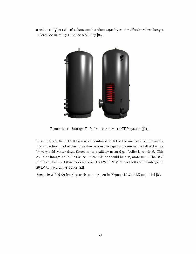
sized on a higher ratio of volume against plant capacity can be e�ective when changes
in loads occur many times across a day [96].
Figure 4.1.1: Storage Tank for use in a micro-CHP system ([31])
In some cases the fuel cell even when combined with the thermal tank cannot satisfy
the whole heat load of the house due to possible rapid increases in the DHW load or
by very cold winter days, therefore an auxiliary natural gas boiler is required. This
could be integrated in the fuel cell micro-CHP or could be a separate unit. The Baxi
Innotech Gamma 1.0 includes a 1 kWe/1.7 kWth PEMFC fuel cell and an integrated
20 kWth natural gas boiler [22].
Some simpli�ed design alternatives are shown in Figures 4.1.2, 4.1.3 and 4.1.4 [2].
58
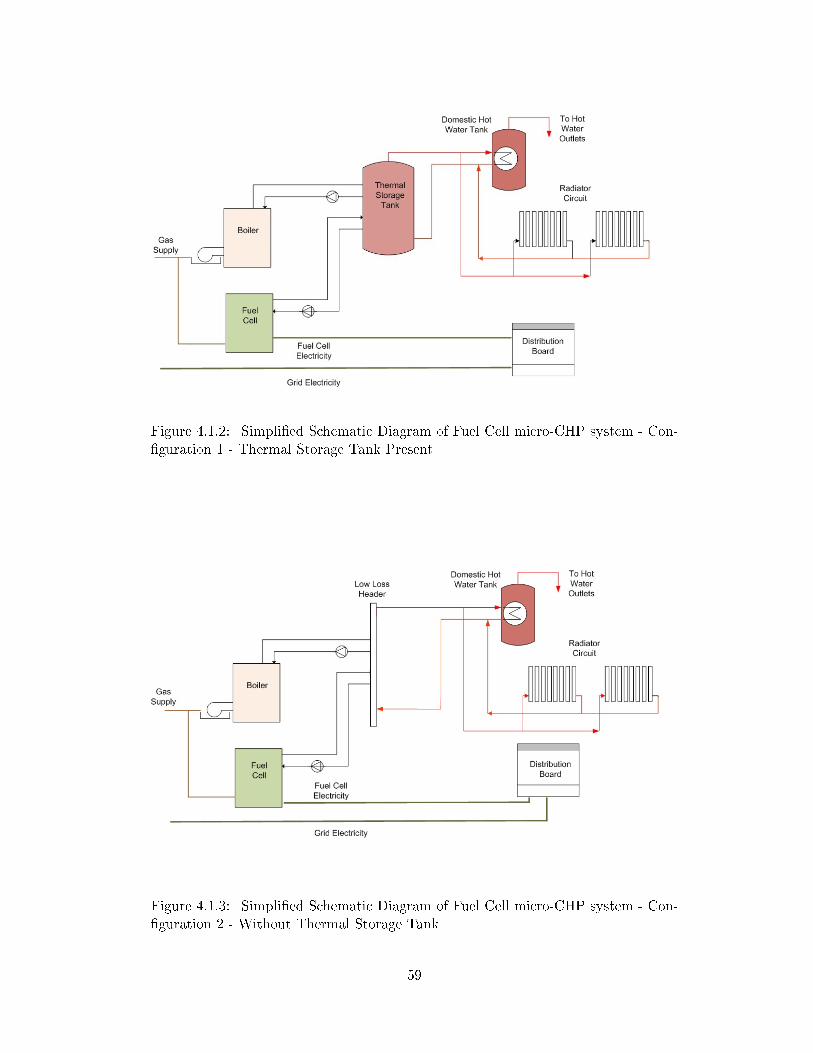
Figure 4.1.2: Simpli�ed Schematic Diagram of Fuel Cell micro-CHP system - Con-�guration 1 - Thermal Storage Tank Present
Figure 4.1.3: Simpli�ed Schematic Diagram of Fuel Cell micro-CHP system - Con-�guration 2 - Without Thermal Storage Tank
59
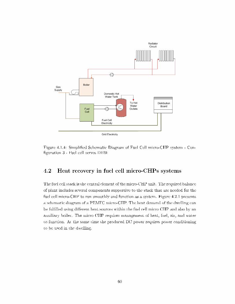
Figure 4.1.4: Simpli�ed Schematic Diagram of Fuel Cell micro-CHP system - Con-�guration 3 - Fuel cell serves DHW
4.2 Heat recovery in fuel cell micro-CHPs systems
The fuel cell stack is the central element of the micro-CHP unit. The required balance
of plant includes several components supportive to the stack that are needed for the
fuel cell micro-CHP to run smoothly and function as a system. Figure 4.2.1 presents
a schematic diagram of a PEMFC micro-CHP. The heat demand of the dwelling can
be ful�lled using di�erent heat sources within the fuel cell micro-CHP and also by an
auxiliary boiler. The micro-CHP requires management of heat, fuel, air, and water
to function. At the same time the produced DC power requires power conditioning
to be used in the dwelling.
60
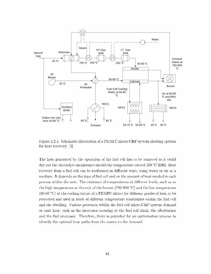
�
Natural Gas
Anode
Cathode
Reformer
Air Preheater
Air Blower
Air at 60-80 °C and 80%
RH
Fuel Cell Cooling Water at 60-80
°C
Exhaust
HEX1HEX2 HEX3
Exhaust Gases at 750-850
oC
55-75 °C 50-65 °C 40 °C 30 °C
90 °C 80 °C
25 °C700 °C 60-80 °C
60-80 °C
HT Gas Shift
LT Gas Shift
400 °C
Water
Steam
200 oC
25 °C
Auxiliary Boiler
Output can vary from 40-90 oC
Burner
Figure 4.2.1: Schematic illustration of a PEMFC micro-CHP system showing optionsfor heat recovery. [2]
The heat generated by the operation of the fuel cell has to be removed as it could
dry out the electrolyte membranes should the temperature exceed 100 °C [130]. Heat
recovery from a fuel cell can be performed in di�erent ways, using water or air as a
medium. It depends on the type of fuel cell and on the amount of heat needed in each
process within the unit. The existance of temperatures at di�erent levels, such as as
the high temperature at the exit of the burner (700-900 °C) and the low temperature
(60-80 °C) at the cooling circuit of a PEMFC allows for di�erent grades of heat to be
recovered and used in loads of di�erent temperature constraints within the fuel cell
and the dwelling. Various processes within the fuel cell micro-CHP system demand
or emit heat, such as the processes occuring at the fuel cell stack, the afterburner
and the fuel processor. Therefore, there is potential for an optimisation process to
identify the optimal heat paths from the source to the demand.
61
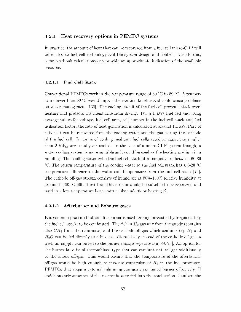
4.2.1 Heat recovery options in PEMFC systems
In practice, the amount of heat that can be recovered from a fuel cell micro-CHP will
be related to fuel cell technology and the system design and control. Despite this,
some textbook calculations can provide an approximate indication of the available
resource.
4.2.1.1 Fuel Cell Stack
Conventional PEMFCs work in the temperature range of 60 °C to 80 °C. A temper-
ature lower than 60 °C would impact the reaction kinetics and could cause problems
on water management [130]. The cooling circuit of the fuel cell prevents stack over-
heating and protects the membrane from drying. For a 1 kWe fuel cell and using
average values for voltage, fuel cell area, cell number in the fuel cell stack and fuel
utilisation factor, the rate of heat generation is calculated at around 1.1 kW. Part of
this heat can be recovered from the cooling water and the gas exiting the cathode
of the fuel cell. In terms of cooling medium, fuel cells rated at capacities smaller
than 2 kWth are usually air cooled. In the case of a micro-CHP system though, a
water cooling system is more suitable as it could be used as the heating medium in a
building. The cooling water exits the fuel cell stack at a temperature between 60-80
°C. The return temperature of the cooling water to the fuel cell stack has a 5-20 °C
temperature di�erence to the water exit temperature from the fuel cell stack [70].
The cathode o�-gas stream consists of humid air at 80%-100% relative humidity at
around 60-80 °C [89]. Heat from this stream would be suitable to be recovered and
used in a low temperature heat emitter like under�oor heating [2].
4.2.1.2 Afterburner and Exhaust gases
It is common practise that an afterburner is used for any unreacted hydrogen exiting
the fuel cell stack, to be combusted. The rich in H2 gas mix from the anode (contains
also CH4 from the reformate) and the cathode o�-gas which contains O2, N2 and
H2O can be fed directly to a burner. Alternatively instead of the cathode-o� gas, a
fresh air supply can be fed to the burner using a separate fan [89, 93]. An option for
the burner is to be of thecombined type that can combust natural gas additionally
to the anode o�-gas. This would ensure that the temperature of the afterburner
o�-gas would be high enough to increase conversion of H2 in the fuel processor.
PEMFCs that require external reforming can use a combined burner e�ectively. If
stoichiometric amounts of the reactants were fed into the combustion chamber, the
62
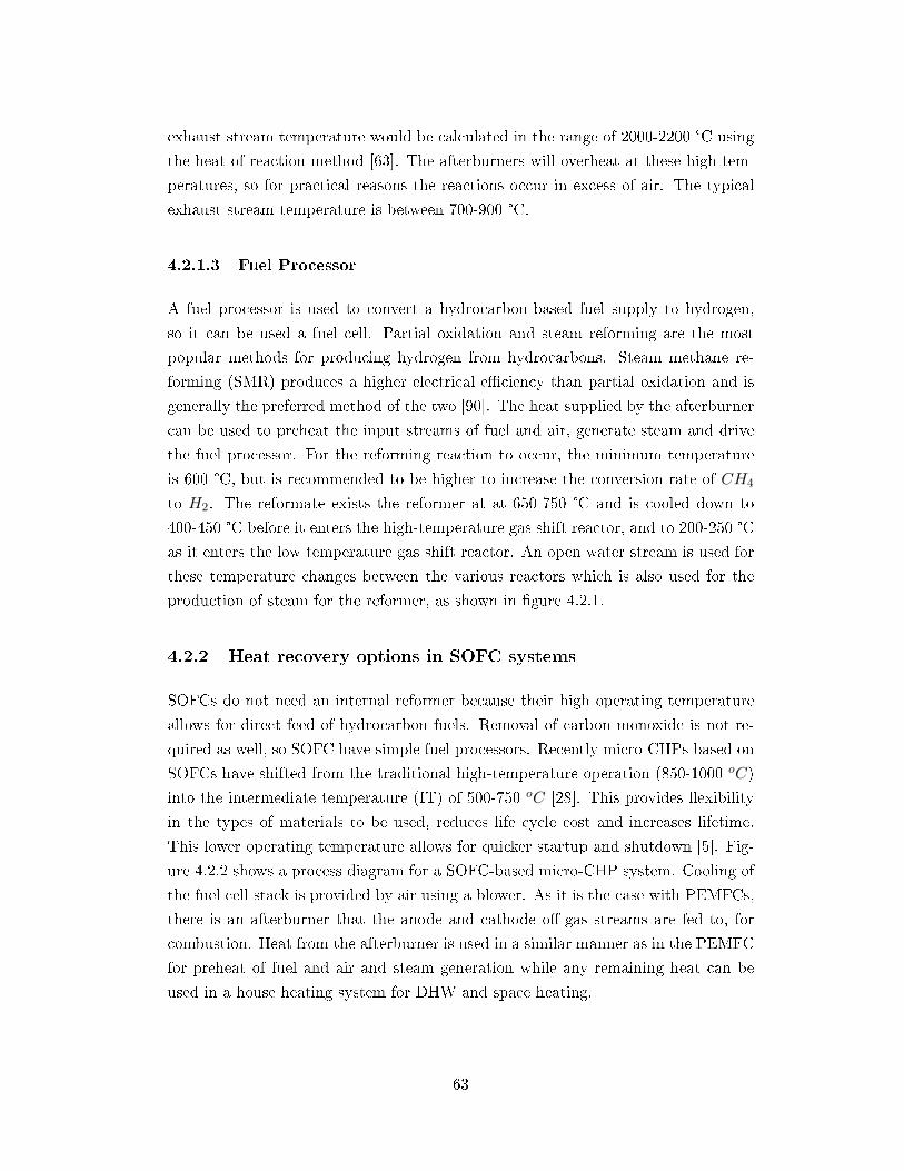
exhaust stream temperature would be calculated in the range of 2000-2200 °C using
the heat of reaction method [63]. The afterburners will overheat at these high tem-
peratures, so for practical reasons the reactions occur in excess of air. The typical
exhaust stream temperature is between 700-900 °C.
4.2.1.3 Fuel Processor
A fuel processor is used to convert a hydrocarbon-based fuel supply to hydrogen,
so it can be used a fuel cell. Partial oxidation and steam reforming are the most
popular methods for producing hydrogen from hydrocarbons. Steam methane re-
forming (SMR) produces a higher electrical e�ciency than partial oxidation and is
generally the preferred method of the two [90]. The heat supplied by the afterburner
can be used to preheat the input streams of fuel and air, generate steam and drive
the fuel processor. For the reforming reaction to occur, the minimum temperature
is 600 °C, but is recommended to be higher to increase the conversion rate of CH4
to H2. The reformate exists the reformer at at 650-750 °C and is cooled down to
400-450 °C before it enters the high-temperature gas shift reactor, and to 200-250 °C
as it enters the low temperature gas shift reactor. An open water stream is used for
these temperature changes between the various reactors which is also used for the
production of steam for the reformer, as shown in �gure 4.2.1.
4.2.2 Heat recovery options in SOFC systems
SOFCs do not need an internal reformer because their high operating temperature
allows for direct feed of hydrocarbon fuels. Removal of carbon monoxide is not re-
quired as well, so SOFC have simple fuel processors. Recently micro-CHPs based on
SOFCs have shifted from the traditional high-temperature operation (850-1000 oC)
into the intermediate temperature (IT) of 500-750 oC [28]. This provides �exibility
in the types of materials to be used, reduces life cycle cost and increases lifetime.
This lower operating temperature allows for quicker startup and shutdown [5]. Fig-
ure 4.2.2 shows a process diagram for a SOFC-based micro-CHP system. Cooling of
the fuel cell stack is provided by air using a blower. As it is the case with PEMFCs,
there is an afterburner that the anode and cathode o�-gas streams are fed to, for
combustion. Heat from the afterburner is used in a similar manner as in the PEMFC
for preheat of fuel and air and steam generation while any remaining heat can be
used in a house heating system for DHW and space heating.
63
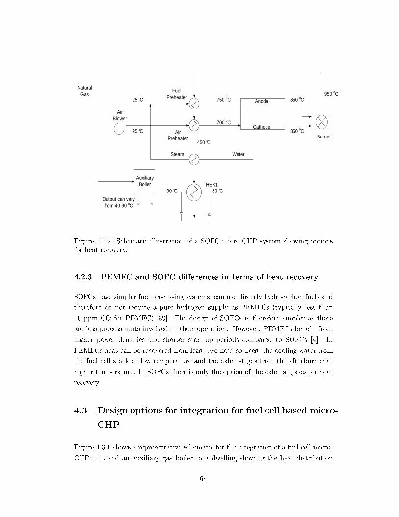
�
Natural Gas
Anode
Cathode
Fuel Preheater
Air Preheater
Air Blower
HEX190 °C 80 °C
25 °C
700 oC
25 °C
Auxiliary Boiler
Output can vary from 40-90 oC
750 oC
Water Steam
850 oC950 oC
850 oC
450 °CBurner
Figure 4.2.2: Schematic illustration of a SOFC micro-CHP system showing optionsfor heat recovery.
4.2.3 PEMFC and SOFC di�erences in terms of heat recovery
SOFCs have simpler fuel processing systems, can use directly hydrocarbon fuels and
therefore do not require a pure hydrogen supply as PEMFCs (typically less than
10 ppm CO for PEMFC) [89]. The design of SOFCs is therefore simpler as there
are less process units involved in their operation. However, PEMFCs bene�t from
higher power densities and shorter start-up periods compared to SOFCs [4]. In
PEMFCs heat can be recovered from least two heat sources: the cooling water from
the fuel cell stack at low temperature and the exhaust gas from the afterburner at
higher temperature. In SOFCs there is only the option of the exhaust gases for heat
recovery.
4.3 Design options for integration for fuel cell based micro-
CHP
Figure 4.3.1 shows a representative schematic for the integration of a fuel cell micro-
CHP unit and an auxiliary gas boiler to a dwelling showing the heat distribution
64
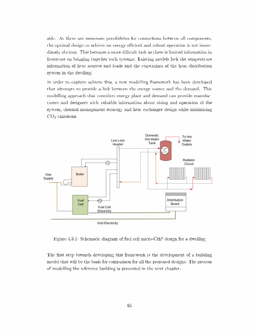
side. As there are numerous possibilities for connections between all components,
the optimal design to achieve an energy e�cient and robust operation is not imme-
diately obvious. This becomes a more di�cult task as there is limited information in
literature on bringing together such systems. Existing models lack the temperature
information of heat sources and loads and the constraints of the heat distribution
system in the dwelling.
In order to capture achieve this, a new modelling framework has been developed
that attempts to provide a link between the energy source and the demand. This
modelling approach that considers energy plant and demand can provide manufac-
turers and designers with valuable information about sizing and operation of the
system, thermal management strategy and heat exchanger design while minimizing
CO2 emissions.
Fuel Cell
Boiler
Domestic Hot Water
Tank
Radiator Circuit
To Hot Water Outlets
Low Loss Header
Distribution Board
Gas Supply
Fuel Cell Electricity
Grid Electricity
Figure 4.3.1: Schematic diagram of fuel cell micro-CHP design for a dwelling
The �rst step towards developing this framework is the development of a building
model that will be the basis for comparison for all the proposed designs. The process
of modelling the reference building is presented in the next chapter.
65
Chapter 5
Reference Building and Dwelling
Energy Data
5.1 Reference Building
Energy demand data for dwellings that include heating, domestic hot water and elec-
tricity information can either be obtained by using Building Information Modelling
(BIM) or can be obtained from real houses from various sources. A source for such
data is the English Housing Survey, which is a survey of English houses and provides
information of the condition and energy e�ciency [42].
All the case studies that are presented in this thesis are compared against a refer-
ence building. The reference dwelling has been developed according to the existing
literature and own interpretation. The reference building is modelled with building
modelling software and is a house served by a conventional heating and electricity
system. It is considered that using modelling data for the house energy demand
instead of existing consumption data would provide �clean� data that can easily be
used in the next steps. Real data require attention as they can be in�uenced by
unknown factors such as the accuracy of sensors, occupants etc. For the purposes of
the model a robust data set was needed to develop the methodology. It was decided
that such dataset can be obtained using building information modelling.
Overall there are two reference buildings de�ned here. They share the same shape,
size and area but di�er on the energy characteristics. The building is located in
London and is a four bedroom house with two storeys; a total �oor area of about
190 m2. A large house with higher energy requirements is be able to identify more
clearly the characteristics of the proposed solutions. House A is a building which
66
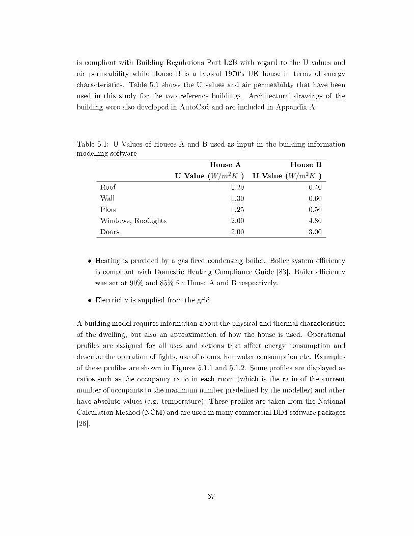
is compliant with Building Regulations Part L2B with regard to the U values and
air permeability while House B is a typical 1970's UK house in terms of energy
characteristics. Table 5.1 shows the U values and air permeability that have been
used in this study for the two reference buildings. Architectural drawings of the
building were also developed in AutoCad and are included in Appendix A.
Table 5.1: U Values of Houses A and B used as input in the building informationmodelling software
House A House B
U Value (W/m2K ) U Value (W/m2K )
Roof 0.20 0.40
Wall 0.30 0.60
Floor 0.25 0.50
Windows, Roo�ights 2.00 4.80
Doors 2.00 3.00
� Heating is provided by a gas �red condensing boiler. Boiler system e�ciency
is compliant with Domestic Heating Compliance Guide [83]. Boiler e�ciency
was set at 90% and 85% for House A and B respectively.
� Electricity is supplied from the grid.
A building model requires information about the physical and thermal characteristics
of the dwelling, but also an approximation of how the house is used. Operational
pro�les are assigned for all uses and actions that a�ect energy consumption and
describe the operation of lights, use of rooms, hot water consumption etc. Examples
of these pro�les are shown in Figures 5.1.1 and 5.1.2. Some pro�les are displayed as
ratios such as the occupancy ratio in each room (which is the ratio of the current
number of occupants to the maximum number prede�ned by the modeller) and other
have absolute values (e.g. temperature). These pro�les are taken from the National
Calculation Method (NCM) and are used in many commercial BIM software packages
[26].
67
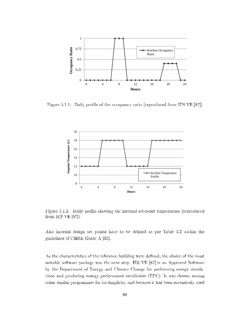
0
0.25
0.5
0.75
1
0 4 8 12 16 20 24
Occ
upan
cy R
atio
Hours
Kitchen OccupancyRatio
Figure 5.1.1: Daily pro�le of the occupancy ratio (reproduced from IES VE [87])
8
10
12
14
16
18
20
0 4 8 12 16 20 24
Setp
oint
Tem
pera
ture
(C
)
Hours
Kitchen TemperatureProfile
Figure 5.1.2: Daily pro�le showing the internal set-point temperature (reproducedfrom IES VE [87])
Also internal design set points have to be de�ned as per Table 5.2 within the
guidelines of CIBSE Guide A [37].
As the characteristics of the reference building were de�ned, the choice of the most
suitable software package was the next step. IES VE [87] is an Approved Software
by the Department of Energy and Climate Change for performing energy simula-
tions and producing energy performance certi�cates (EPC). It was chosen among
other similar programmes for its simplicity and because it has been extensively used
68
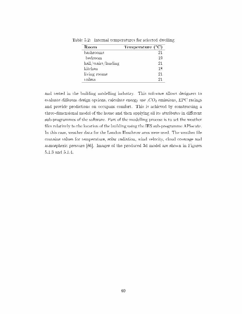
Table 5.2: Internal temperatures for selected dwelling
Room Temperature (°C)
bathrooms 21bedroom 19hall/stairs/landing 21kitchen 18living rooms 21toilets 21
and tested in the building modelling industry. This software allows designers to
evaluate di�erent design options, calculate energy use ,CO2 emissions, EPC ratings
and provide predictions on occupant comfort. This is achieved by constructing a
three-dimensional model of the house and then applying all its attributes in di�erent
sub-programmes of the software. Part of the modelling process is to set the weather
�les relatively to the location of the building using the IES sub-programme APlocate.
In this case, weather data for the London Heathrow area were used. The weather �le
contains values for temperature, solar radiation, wind velocity, cloud coverage and
atmospheric pressure [86]. Images of the produced 3d model are shown in Figures
5.1.3 and 5.1.4.
69
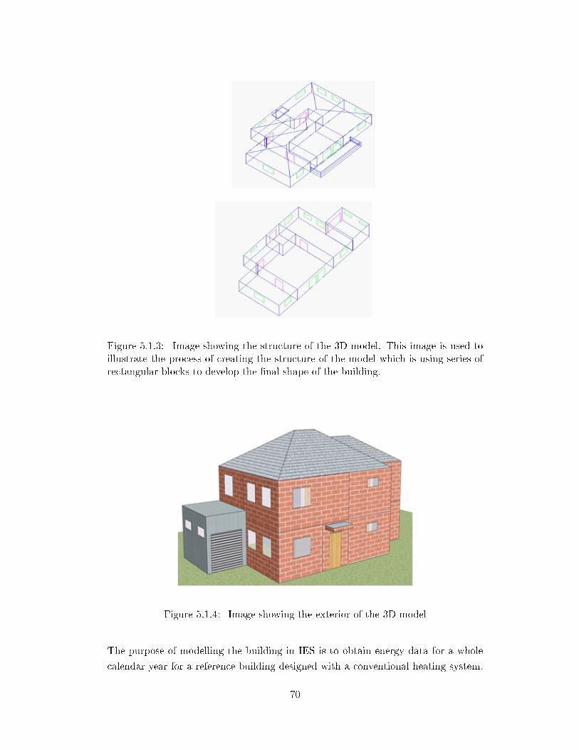
Figure 5.1.3: Image showing the structure of the 3D model. This image is used toillustrate the process of creating the structure of the model which is using series ofrectangular blocks to develop the �nal shape of the building.
Figure 5.1.4: Image showing the exterior of the 3D model
The purpose of modelling the building in IES is to obtain energy data for a whole
calendar year for a reference building designed with a conventional heating system.
70
The heat demand is a function of the outside temperature, the U Values, the internal
set-point temperatures and their use pro�les. The data presented in section 5.2 will
be used as the basis for comparison of fuel cell micro-CHP designs and conventional
systems for residential applications.
The choice of a new Part L compliant dwelling and an older typical UK dwelling
ensures that the studies presented can capture a wide range of the UK building stock.
It will then be feasible to extract conclusions about the feasibility of the studies on
a larger scale without being limited by the scope of a single case study.
5.2 Dwelling Energy Data
This chapter presents the energy demand data for heating, DHW and electricity
for Houses A and B. The loads di�er according to the di�erent heat emitters for
both houses. The base case for all examples presented represents a dwelling that is
designed with a natural gas boiler to satisfy heating and hot water requirements and
is connected to the electricity grid. The dataset obtained contains yearly data with
5 minute timesteps. However, as this results in a large number of data, a 1 hour
timestep has been used throughout.
The complete yearly dataset of 8760 hours is presented here. It is then used to
extract segments and to create subsets to examine various case studies presented in
Chapters 6 and 7. Subsets could be single winter or summer days comprised of 24
hours or larger.
Figure 5.2.1 shows the 24-hour heat demand of the DHW tank. This is to main-
tain water in the storage tank at 60 °C at all times. It takes into account the
hot water consumption pro�le of the occupants and storage losses at a rate of
0.0075 kWh/lday. Modelling the DHW system has been carried out using IES's
sub-programme ApacheView [85] . It remains unchanged for both houses regardless
of the choice of heating system and follows a 24-hour pattern that repeats through-
out the year. The DHW demand peaks in the morning when typically people have
showers and also in the evening hours when people typically return from work and
occupancy increases.
Figure 5.2.2 shows the electricity demand which follows a weekly repetitive pattern
with higher demand on weekends. This weekly pattern is the repeated throughout
the year. The increased demand in weekends can be explained by the additional
electricity load for lights and electronic devices during weekends because of the in-
creased occupancy. At the same time, on a daily basis the electricity demand follows
71

the occupancy pattern with morning and late afternoon peaks.
0 6 1 2 1 8 2 40
1
2
3He
at (kW
)
T i m e ( H r s )
D H W S y s t e m
Figure 5.2.1: Graph representing the 24-hour heat demand for DHW pattern forthe reference dwelling. The graph shows the relation between the occupancy, whichis high in the morning and in the evening hours, and the DHW demand.
72

0 2 4 4 8 7 2 9 6 1 2 0 1 4 4 1 6 80
1
2
Electr
icity (
kW)
T i m e ( H r s )
E l e c t r i c i t y D e m a n d
Figure 5.2.2: Graph representing the weekly electricity demand for House A. Thisweekly electricity pattern repeats throughout the year and peaks in the weekends.
5.2.1 House A - Part L Building
5.2.1.1 UFH System
The maximum space heating load for the UFH system is 7.9 kW which is a low value
considering the area of the house. However, the low U-Values and air permeability
that are in line with Part L regulations results an e�cient system with lower heat
demand.
The UFH is generally a slow response system that requires longer heating hours and
less peaks compared to a radiator system. The space heating demand for House A
served by under�oor heating can be seen in Figure 5.2.3.
73
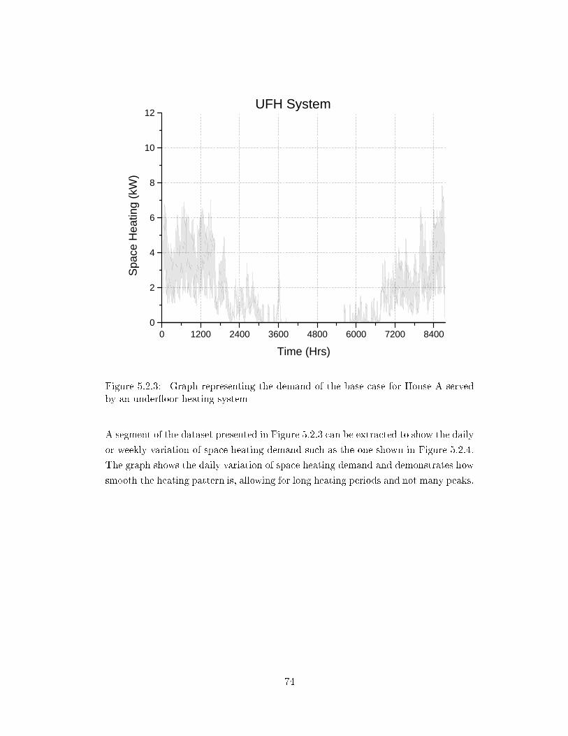
0 1 2 0 0 2 4 0 0 3 6 0 0 4 8 0 0 6 0 0 0 7 2 0 0 8 4 0 00
2
4
6
8
1 0
1 2Sp
ace H
eatin
g (kW
)
T i m e ( H r s )
U F H S y s t e m
Figure 5.2.3: Graph representing the demand of the base case for House A servedby an under�oor heating system
A segment of the dataset presented in Figure 5.2.3 can be extracted to show the daily
or weekly variation of space heating demand such as the one shown in Figure 5.2.4.
The graph shows the daily variation of space heating demand and demonstrates how
smooth the heating pattern is, allowing for long heating periods and not many peaks.
74
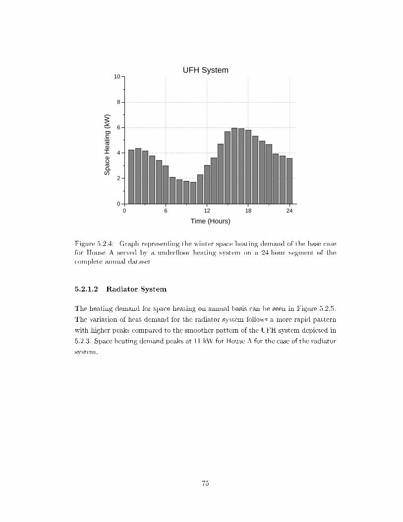
0 6 1 2 1 8 2 40
2
4
6
8
1 0
Spac
e Hea
ting (
kW)
T i m e ( H o u r s )
U F H S y s t e m
Figure 5.2.4: Graph representing the winter space heating demand of the base casefor House A served by a under�oor heating system on a 24-hour segment of thecomplete annual dataset
5.2.1.2 Radiator System
The heating demand for space heating on annual basis can be seen in Figure 5.2.5.
The variation of heat demand for the radiator system follows a more rapid pattern
with higher peaks compared to the smoother pattern of the UFH system depicted in
5.2.3. Space heating demand peaks at 11 kW for House A for the case of the radiator
system.
75
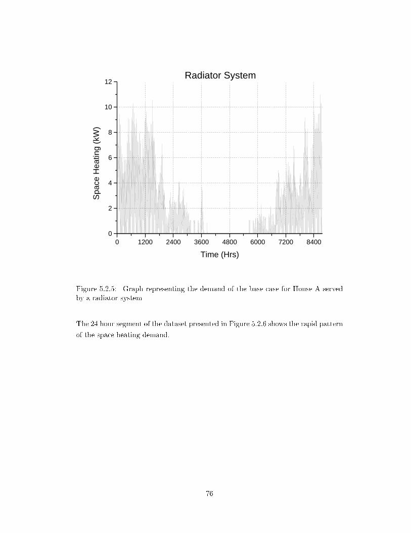
0 1 2 0 0 2 4 0 0 3 6 0 0 4 8 0 0 6 0 0 0 7 2 0 0 8 4 0 00
2
4
6
8
1 0
1 2Sp
ace H
eatin
g (kW
)
T i m e ( H r s )
R a d i a t o r S y s t e m
Figure 5.2.5: Graph representing the demand of the base case for House A servedby a radiator system
The 24 hour segment of the dataset presented in Figure 5.2.6 shows the rapid pattern
of the space heating demand.
76
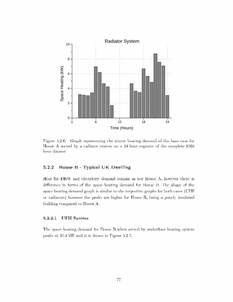
0 6 1 2 1 8 2 40
2
4
6
8
1 0
Spac
e Hea
ting (
kW)
T i m e ( H o u r s )
R a d i a t o r S y s t e m
Figure 5.2.6: Graph representing the winter heating demand of the base case forHouse A served by a radiator system on a 24-hour segment of the complete 8760hour dataset
5.2.2 House B - Typical UK Dwelling
Heat for DHW and electricity demand remain as per House A, however there is
di�erence in terms of the space heating demand for House B. The shape of the
space heating demand graph is similar to the respective graphs for both cases (UFH
or radiators) however the peaks are higher for House B, being a poorly insulated
building compared to House A.
5.2.2.1 UFH System
The space heating demand for House B when served by under�oor heating system
peaks at 31.4 kW and it is shown in Figure 5.2.7.
77

0 1 2 0 0 2 4 0 0 3 6 0 0 4 8 0 0 6 0 0 0 7 2 0 0 8 4 0 00
1 0
2 0
3 0
4 0Sp
ace H
eatin
g (kW
)
T i m e ( H r s )
U F H S y s t e m
Figure 5.2.7: Graph representing the demand of the base case for House B servedby an under�oor heating system
5.2.2.2 Radiator System
The variation of the heating and electricity load for House B is shown in Figure 5.2.8.
The heating demand for the poorly insulated building peaks at 44.1 kW.
78
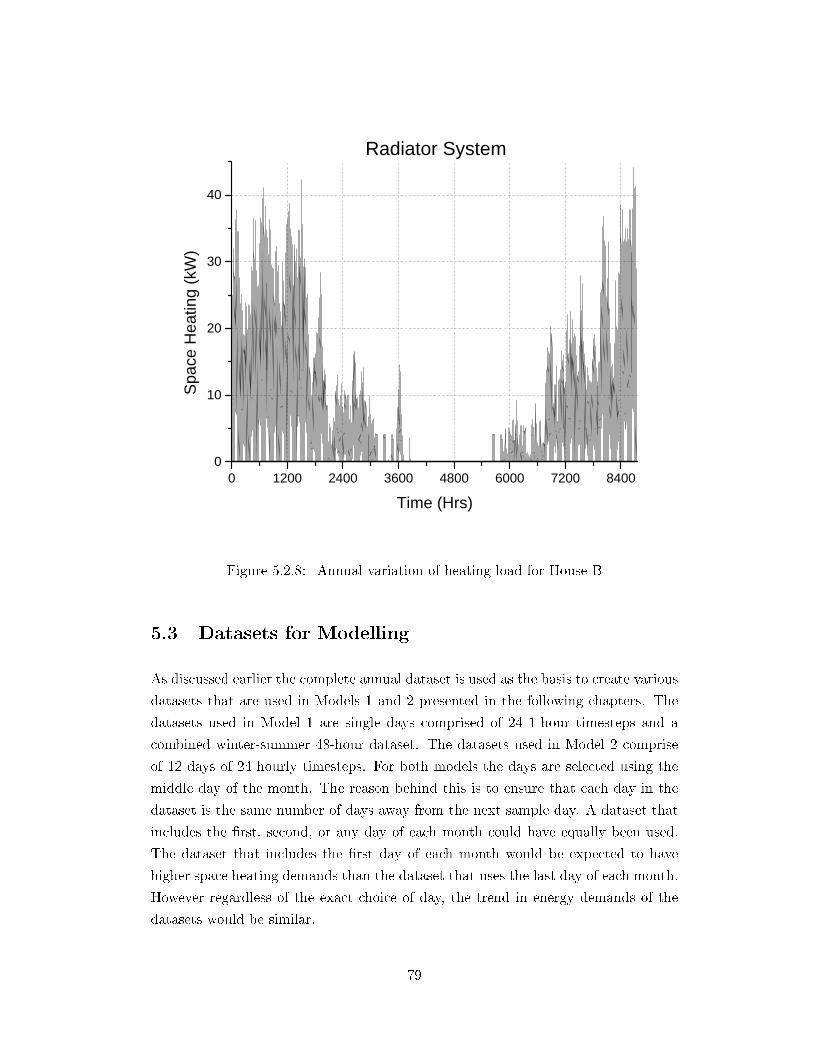
0 1 2 0 0 2 4 0 0 3 6 0 0 4 8 0 0 6 0 0 0 7 2 0 0 8 4 0 00
1 0
2 0
3 0
4 0Sp
ace H
eatin
g (kW
)
T i m e ( H r s )
R a d i a t o r S y s t e m
Figure 5.2.8: Annual variation of heating load for House B
5.3 Datasets for Modelling
As discussed earlier the complete annual dataset is used as the basis to create various
datasets that are used in Models 1 and 2 presented in the following chapters. The
datasets used in Model 1 are single days comprised of 24 1-hour timesteps and a
combined winter-summer 48-hour dataset. The datasets used in Model 2 comprise
of 12 days of 24 hourly timesteps. For both models the days are selected using the
middle day of the month. The reason behind this is to ensure that each day in the
dataset is the same number of days away from the next sample day. A dataset that
includes the �rst, second, or any day of each month could have equally been used.
The dataset that includes the �rst day of each month would be expected to have
higher space heating demands than the dataset that uses the last day of each month.
However regardless of the exact choice of day, the trend in energy demands of the
datasets would be similar.
79
As each day in the dataset represents one month, the developed datasets might not
contain data for the coldest day of the year. At �rst this might suggest that the
proposed designs might not be able to meet the heating load of the dwelling at
the particular day. However in reality the results that can be obtained from a a
modelling study would require interpretation and assessment before proceeding to
plant selection. Extra plant capacity is added to the calculated to shorten the preheat
period of the heating space in cases of the heating being turned o� for a big period of
time [96]. At the same time there is uncertainty already involved on the accuracy of
the heating load calculation caused by assumptions while estimating the U-values.
According to Biddulph et al. �Unfortunately the actual U-value may be di�erent
from those values obtained using assumptions about the materials, their properties
and the structure of the wall after a cursory visual inspection.� [25]. The heat
demand is related to the users of the building, their perception of thermal comfort
and their behaviour in terms of the way they operate the room thermostat which
could be completely unpredictable. Therefore developing a smaller dataset that can
describe the heat demand of a whole year cannot be done without a compromise. The
developed datasets are used in the models to identify trends and patterns for decision
variables. The concept of identifying trends in the resulting designs is behind the
consideration of di�erent scenarios and buildings in the models presented.
Another issue with regard to the developed datasets is the e�ect of the temporal
precision. The idea of having a 1-hour timestep allows for smaller datasets that can
capture a whole year cycle without having to use too many data. However, there
is information lost as the variations of energy demand during this hourly period
are averaged on the 1-hour timestep. That could lead to lower maximum values
for heating or electricity loads that are to be met and therefore variations in the
conclusions about overall primary energy reductions o�ered by a system. This view
is supported by Hawkes et al. �...coarse temporal precision leads to averaging e�ects
that result in misleading environmental and economic outcomes for cost-optimal
micro-CHP systems� [71]. Napoli et al. suggests that when modelling micro-CHP
systems, the electrical pro�les may need higher temporal precision than the heating
ones as as the presence of a thermal storage tank will smoothen the heating load
[93]. An implication of using averaged 1-hour timesteps is that the ramping and
capacity constraints that de�ne the performance of the fuel cell micro-CHP would
have less signi�cance in a model compared to a more detailed dataset that uses 5-
minute timesteps. As a result the choice of 1-hour timesteps in the input energy data
of the models might lead to results that favour electricity generation from the fuel
cell micro-CHP while also underestimating the total CO2 emissions of the systems.
80
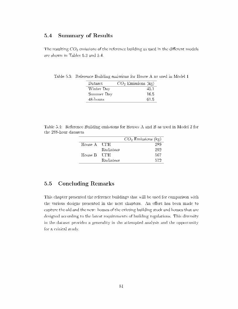
5.4 Summary of Results
The resulting CO2 emissions of the reference building as used in the di�erent models
are shown in Tables 5.3 and 5.4.
Table 5.3: Reference Building emissions for House A as used in Model 1
Dataset CO2 Emissions (kg)Winter Day 45.1Summer Day 16.548-hours 61.5
Table 5.4: Reference Building emissions for Houses A and B as used in Model 2 forthe 288-hour datasets
CO2 Emissions (kg)House A UFH 289
Radiators 292House B UFH 567
Radiators 572
5.5 Concluding Remarks
This chapter presented the reference buildings that will be used for comparison with
the various designs presented in the next chapters. An e�ort has been made to
capture the old and the new: houses of the existing building stock and houses that are
designed according to the latest requirements of building regulations. This diversity
in the dataset provides a generality in the attempted analysis and the opportunity
for a critical study.
81
Chapter 6
Model 1 - An MINLP model for
high level evaluation of a SOFC
micro-CHP design in dwellings
This model attempts to identify optimal designs in terms of CO2 emissions for SOFC
based fuel cell micro-CHP in dwellings without using any electrochemistry equations.
The methodology is treating all plant as �black boxes� with e�ciencies assigned to
them and considers DHW and space heating as one demand. The purpose of the
model is to provide a simple tool for a high level evaluation of a fuel cell micro-CHP
design that can be used in the early stages.
Part of the work presented in this chapter has been published in [3].
6.1 Optimisation methods in energy systems
As part of this PhD project optimisation techniques have been used. The exact
methodology will be explained in detail later, however the purpose of this chapter is
to summarise the key features of optimisation that are relevant to the study.
In an optimisation problem a mathematical model of the system has to be formulated.
The model consists of the following elements:
1. Variables,
2. Parameters,
3. Constraints, and
82
4. Mathematical Relationships
A de�nition of any optimisation problem is the following:
maximise/minimize f(x) (6.1.1)
with
x = (x1, x2, ..., xn) (6.1.2)
subject to the equality and inequality constraints
hi(x) = 0 i=(1,2,...,k)
gj(x) ≤ 0 j=(1,2,...,l)
In the case of optimisation in the built environment involving micro-CHP plant the
objective function could be the total cost (capital or operational), the total energy
consumption (or CO2 emissions) of the system, the e�ciency etc. The variables
involved could represent the energy output of each source and the capacity of each
plant. The parameters could be energy requirement data, cost information (i.e ¿
per kWh of imported electricity) etc. Constraints are usually energy balances or
technical constraints of the plant involved.
An optimal solution of a problem contains values for the variables that satisfy the
constraints while optimising the objective function.
The models that will be presented here are primarily MINLP as non-linear terms are
used in e�ciency or energy balance equations that describe the systems. The most
common method implemented to solve MINLP models is the Branch and Bound
method (BB) [53].
Software package for modelling and solving optimisation problems has been de-
veloped over the last 15-20 years and is available either free or as commercial
product. The more widely used include GAMS (General Algebraic Modelling Sys-
tem), AIMMS, Matlab and others [6, 29, 91].
83

6.2 Problem Statement
The overall problem for the high level design of a SOFC micro-CHP in a dwelling
can be stated as follows.
Given:
� Known availability of heat an electricity generating plant ( j : fc,gb) ;
� The total heat (space heating and DHW combined) and electricity demand for
a dwelling (k: heat,ele);
� Process limitations and constraints in terms of energy generation
Determine:
� The sizing and operational characteristics of this design.
So as to minimise the resulting CO2 emissions from the dwelling energy system.
6.3 Basis for the Model
The model overview can be seen in Figure 6.3.1. Natural gas and grid electricity are
the energy inputs of the system, while CO2 emissions the output. The fuel cell is
supplying heat to the TST and from the TST heat can be supplied to the dwelling
for space heating and DHW. An auxiliary gas boiler is supplementing the fuel cell
and TST with heat. Electricity is served by the fuel cell and grid electricity. The
total heat and electricity demand need to be satis�ed at all times. There is a single
demand of heat in the model and this is the combined space heating and DHW.
84
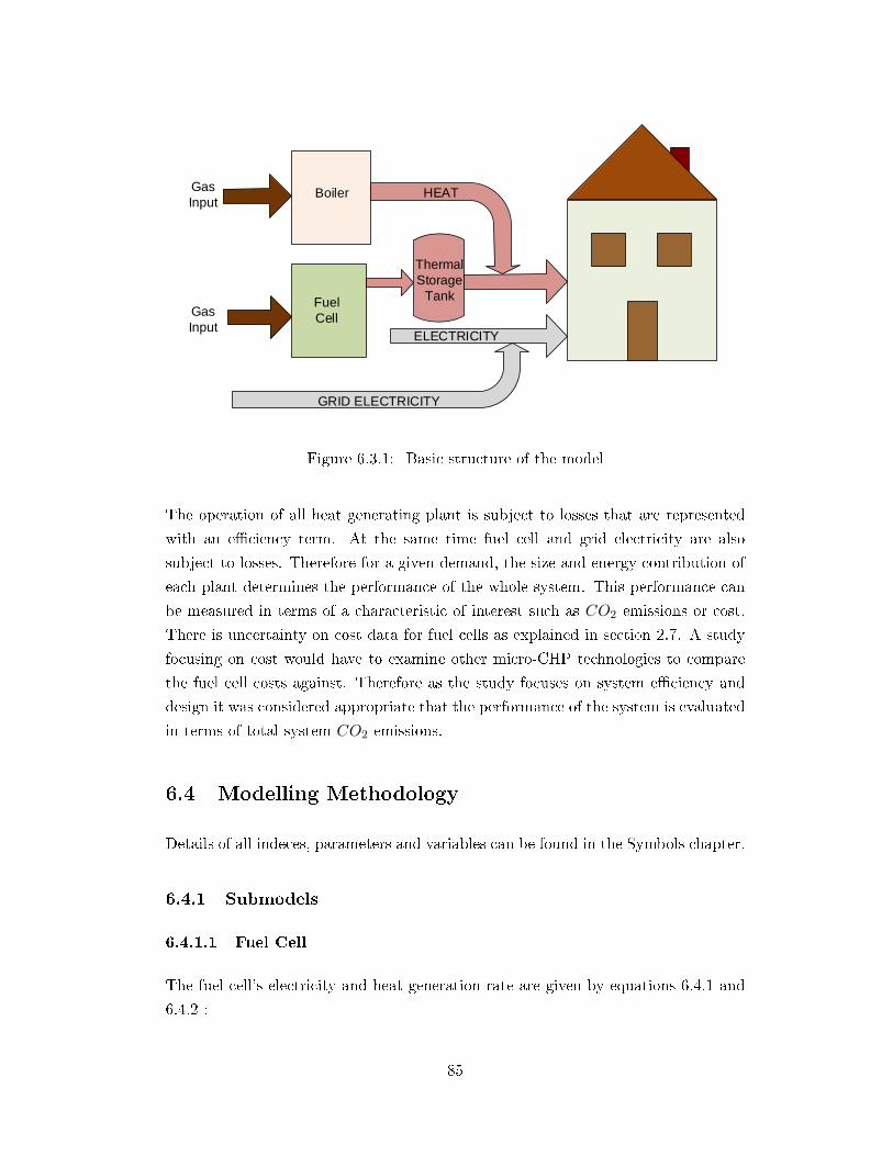
Fuel Cell
BoilerGas Input
ELECTRICITY
Gas Input
HEAT
GRID ELECTRICITY
Thermal Storage
Tank
Figure 6.3.1: Basic structure of the model
The operation of all heat generating plant is subject to losses that are represented
with an e�ciency term. At the same time fuel cell and grid electricity are also
subject to losses. Therefore for a given demand, the size and energy contribution of
each plant determines the performance of the whole system. This performance can
be measured in terms of a characteristic of interest such as CO2 emissions or cost.
There is uncertainty on cost data for fuel cells as explained in section 2.7. A study
focusing on cost would have to examine other micro-CHP technologies to compare
the fuel cell costs against. Therefore as the study focuses on system e�ciency and
design it was considered appropriate that the performance of the system is evaluated
in terms of total system CO2 emissions.
6.4 Modelling Methodology
Details of all indeces, parameters and variables can be found in the Symbols chapter.
6.4.1 Submodels
6.4.1.1 Fuel Cell
The fuel cell's electricity and heat generation rate are given by equations 6.4.1 and
6.4.2 :
85

Qfc,ele(t) = yfc(t) · Pfc · rfc(t) (6.4.1)
Qfc,heat(t) =Qfc,ele(t)
ηfc,ele(t)ηfc,heat(t) (6.4.2)
The variable yj(t) is a binary variable that takes the value 1 when plant j is opera-
tional and 0 when it is o�. Pj represents the maximum capacity in kW and ηj,k(t)
the e�ciency of plant j . Variable Qj,k(t) represents the energy output of plant j
(kW).
The operation of the fuel cell is a�ected by various limitations such as a minimum
turn down ratio. In this study it was set at 20% [77] and the ramp up rate (ra) at
15 We/min or (0.9 kWe/hr ) [75].
0.2Pfc ≤ Qfc,ele(t) ≤ Pfc (6.4.3)
d
dtQfc,ele(t) ≤ ra (6.4.4)
The SOFC micro-CHP converts the chemical energy of the fuel to electricity and
heat according as per its e�ciency. The fuel cell micro-CHP thermal and electrical
e�ciency equations in relation to the load factor rfc(t) are taken from Hawkes et al.
and given by Equations 6.4.5 and 6.4.6 [73].
ηfc,heat(t) = −23.548r6,fc(t) + 131.17r5fc(t)− 295.99r4fc(t)
+355.63r3fc(t)− 251.5r2fc(t) + 121.96rfc(t) (6.4.5)
ηfc,ele(t) = −1065r6fc(t) + 4114.7r5fc(t)− 6437.1r4,fc(t)
+5224.5r3,fc(t)− 2330.7r2fc(t) + 536.81rfc(t) (6.4.6)
6.4.1.2 Gas Boiler
The boiler's heat production rate is given by equation 6.4.7.
Qgb,heat(t) = ygb(t)Pgbrgb(t) (6.4.7)
86

The gas boiler's e�ciency ηgb(t) is set to 90% which is in line with the Domestic
Heating Compliance Guide [83]. In the case of the gas boiler Qgb,ele(t) = 0.
The heat production rate of the boiler is limited by a minimum turn down ratio of
30% and it cannot exceed its maximum capacity:
0.3Pgb ≤ Qgb,heat(t) ≤ Pgb (6.4.8)
6.4.1.3 Thermal Storage Tank
The model for the thermal storage tank includes all energy �ows to/from the TST
and energy balances. The only source of heat for the TST is the fuel cell micro-CHP.
The energy content of the storage tank Est (kJ) is given by equation 6.4.9
Est(t) = V st · ρ · cp · (T st(t)− T emv(t)) (6.4.9)
, where V st (m3) is the storage volume, ρ the water density and T env(t) (oC ) a
reference environmental temperature.
Energy balance in the storage tank is given by equation6.4.10 .
d
dtEst(t) = Qfc,heat(t)−Qstout(t) (6.4.10)
, Qstout(t) (kW) is the heat delivered from the TST to the system and Est(t) energy
content of the storage tank.
Figure 6.4.1 shows the energy �ows of the thermal storage tank.
87
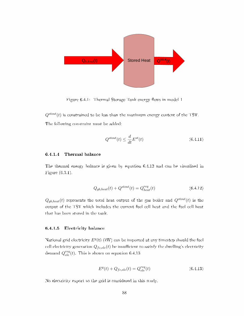
Stored HeatQfc,heat(t) Qstout(t)
Figure 6.4.1: Thermal Storage Tank energy �ows in model 1
Qstout(t) is constrained to be less than the maximum energy content of the TST.
The following constraint must be added:
Qstout(t) ≤ d
dtEst(t) (6.4.11)
6.4.1.4 Thermal balance
The thermal energy balance is given by equation 6.4.12 and can be visualised in
Figure (6.3.1).
Qgb,heat(t) +Qstout(t) = Qreqheat(t) (6.4.12)
Qgb,heat(t) represents the total heat output of the gas boiler and Qstout(t) is the
output of the TST which includes the current fuel cell heat and the fuel cell heat
that has been stored in the tank.
6.4.1.5 Electricity balance
National grid electricity Eg(t) (kW) can be imported at any timestep should the fuel
cell electricity generation Qfc,ele(t) be insu�cient to satisfy the dwelling's electricity
demand Qreqele (t). This is shown on equation 6.4.13
Eg(t) +Qfc,ele(t) = Qreqele (t) (6.4.13)
No electricity export to the grid is considered in this study.
88
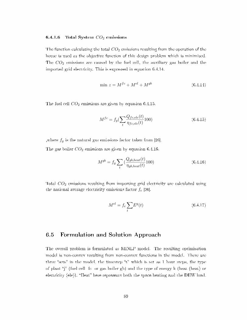
6.4.1.6 Total System CO2 emissions
The function calculating the total CO2 emissions resulting from the operation of the
house is used as the objective function of this design problem which is minimised.
The CO2 emissions are caused by the fuel cell, the auxiliary gas boiler and the
imported grid electricity. This is expressed in equation 6.4.14.
min z = Mfc +M el +Mgb (6.4.14)
The fuel cell CO2 emissions are given by equation 6.4.15.
Mfc = fg(∑t
Qfc,ele(t)
ηfc,ele(t)100) (6.4.15)
,where fg is the natural gas emissions factor taken from [26].
The gas boiler CO2 emissions are given by equation 6.4.16.
Mgb = fg∑t
(Qgb,heat(t)
ηgb,heat(t)100) (6.4.16)
Total CO2 emissions resulting from importing grid electricity are calculated usingthe national average electricity emissions factor fe [26].
M el = fe∑t
Eg(t) (6.4.17)
6.5 Formulation and Solution Approach
The overall problem is formulated as MINLP model. The resulting optimisation
model is non-convex resulting from non-convex functions in the model. There are
three �sets� in the model, the timestep �t� which is set as 1 hour steps, the type
of plant �j� (fuel cell -fc- or gas boiler-gb) and the type of energy k (heat (heat) or
electricity (ele)). �Heat� here represents both the space heating and the DHW load.
89
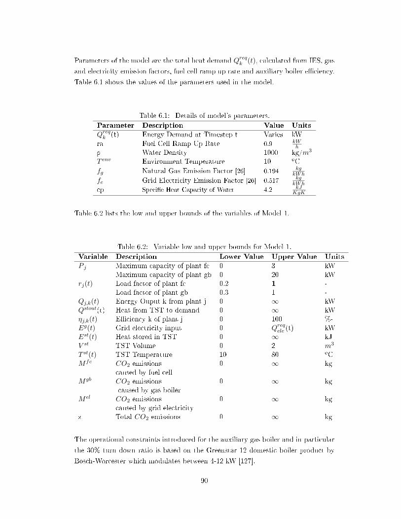
Parameters of the model are the total heat demand Qreqk (t), calculated from IES, gas
and electricity emission factors, fuel cell ramp up rate and auxiliary boiler e�ciency.
Table 6.1 shows the values of the parameters used in the model.
Table 6.1: Details of model's parameters.Parameter Description Value Units
Qreqk (t) Energy Demand at Timestep t Varies kW
ra Fuel Cell Ramp Up Rate 0.9 kWh
ρ Water Density 1000 kg/m3
T env Environment Temperature 10 oCfg Natural Gas Emission Factor [26] 0.194 kg
kWh
fe Grid Electricity Emission Factor [26] 0.517 kgkWh
cp Speci�c Heat Capacity of Water 4.2 kJKgK
Table 6.2 lists the low and upper bounds of the variables of Model 1.
Table 6.2: Variable low and upper bounds for Model 1.Variable Description Lower Value Upper Value Units
P j Maximum capacity of plant fc 0 3 kWMaximum capacity of plant gb 0 20 kW
rj(t) Load factor of plant fc 0.2 1 -Load factor of plant gb 0.3 1 -
Qj,k(t) Energy Ouput k from plant j 0 ∞ kWQstout(t) Heat from TST to demand 0 ∞ kWηj,k(t) E�ciency k of plant j 0 100 %-Eg(t) Grid electricity input 0 Qreq
ele (t) kWEst(t) Heat stored in TST 0 ∞ kJV st TST Volume 0 2 m3
T st(t) TST Temperature 10 80 oCMfc CO2 emissions 0 ∞ kg
caused by fuel cellMgb CO2 emissions 0 ∞ kg
caused by gas boilerM el CO2 emissions 0 ∞ kg
caused by grid electricityz Total CO2 emissions 0 ∞ kg
The operational constraints introduced for the auxiliary gas boiler and in particular
the 30% turn down ratio is based on the Greenstar 12 domestic boiler product by
Bosch-Worcester which modulates between 4-12 kW [127].
90
It was decided that GAMS [29] will be used as the platform of the optimisation
model. GAMS is a modelling tool for mathematical programming and optimisation.
The solver SBB was used for the analysis of this chapter [67]. Other solvers such as
BARON and AlphaECP were evaluated but SBB gave results within the prede�ned
relative optimality gap in a shorter computational time. SBB can achieve better
results than other solvers on smaller models that have di�cult non-linearities which
is the case here [12]. Taking that into account it was decided that SBB will be used.
The SBB solver is built around the Branch and Bound method and a number of NLP
solvers for solving the relaxed NLP submodels. The required time for all solvers to
provide a solution was improved by linearising the e�ciency function as described in
section 6.5.1.
The optimality gap is de�ned as |BP −BF | /BP where BP is the best possible
solution and BF is the best integer solution found by the solver. The optimality
gas was set to 1% for all cases presented in this chapter. For most models a 0%
optimality gap was not feasible and not all case studies could be solved, so a 1% was
the �rst possible gap that provided solutions for all case studies.
It was decided that this analysis will focus on 3 subsets of the complete 8760 hour
yearly dataset presented in Chapter 5.
1. A winter day comprised of 24 timesteps.
2. A summer day comprised of 24 timesteps.
3. A combination of the two above data sets (48 timesteps).
The signi�cance of the weather conditions and associated energy demands can be
observed by carrying out the analysis on these three time periods. Analysing the
winter and summer days separately the design is tested for two di�erent demand
patterns, a high heat-to electricity pattern and a low. The 48-hour analysis would
provide a design proposal that trades o� better than the smaller datasets the di�erent
requirements of the whole year while being a simple model that is easy to converge.
The initial value aspect of the problem and in particular the initial energy level of
the TST can be proved important and in�uence the optimisation results on a 24-
hour dataset as there is a thermal mass stored in the system at the �rst timestep.
This also is valid for the last timestep where any heat stored in the tank will not
be used in the building but has in�uenced the result. This can generally be avoided
by using the complete 8760-hour dataset to reduce the signi�cance of the initial and
�nal values. Alternatively, a constraint can be added that forces the �nal energy
91
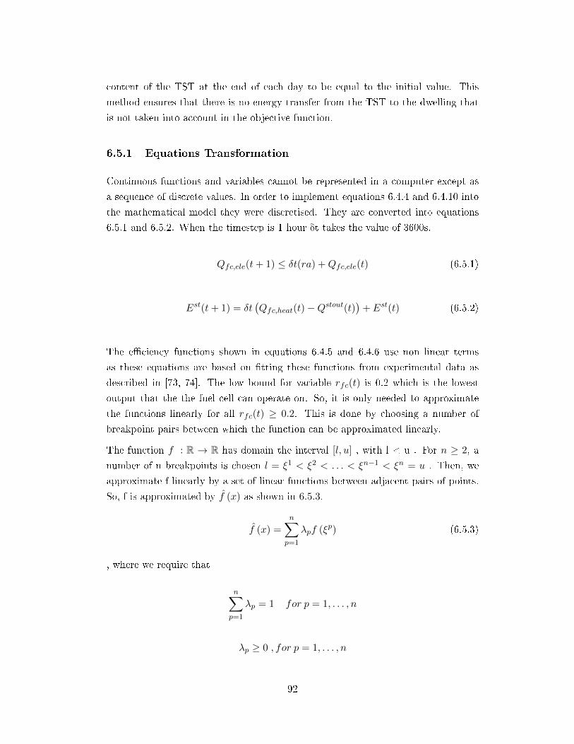
content of the TST at the end of each day to be equal to the initial value. This
method ensures that there is no energy transfer from the TST to the dwelling that
is not taken into account in the objective function.
6.5.1 Equations Transformation
Continuous functions and variables cannot be represented in a computer except as
a sequence of discrete values. In order to implement equations 6.4.4 and 6.4.10 into
the mathematical model they were discretised. They are converted into equations
6.5.1 and 6.5.2. When the timestep is 1 hour δt takes the value of 3600s.
Qfc,ele(t+ 1) ≤ δt(ra) +Qfc,ele(t) (6.5.1)
Est(t+ 1) = δt(Qfc,heat(t)−Qstout(t)
)+ Est(t) (6.5.2)
The e�ciency functions shown in equations 6.4.5 and 6.4.6 use non linear terms
as these equations are based on �tting these functions from experimental data as
described in [73, 74]. The low bound for variable rfc(t) is 0.2 which is the lowest
output that the the fuel cell can operate on. So, it is only needed to approximate
the functions linearly for all rfc(t) ≥ 0.2. This is done by choosing a number of
breakpoint pairs between which the function can be approximated linearly.
The function f : R → R has domain the interval [l, u] , with l < u . For n ≥ 2, a
number of n breakpoints is chosen l = ξ1 < ξ2 < . . . < ξn−1 < ξn = u . Then, we
approximate f linearly by a set of linear functions between adjacent pairs of points.
So, f is approximated by f̂ (x) as shown in 6.5.3.
f̂ (x) =
n∑p=1
λpf (ξp) (6.5.3)
, where we require that
n∑p=1
λp = 1 for p = 1, . . . , n
λp ≥ 0 , for p = 1, . . . , n
92
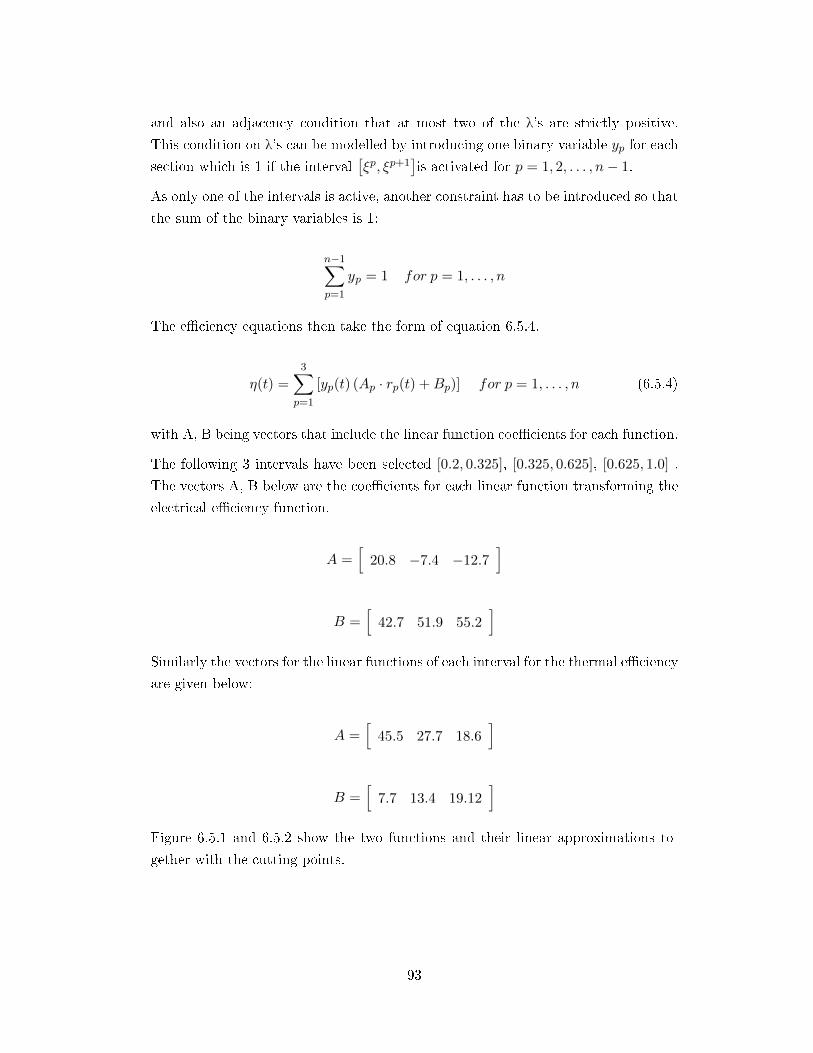
and also an adjacency condition that at most two of the λ's are strictly positive.
This condition on λ's can be modelled by introducing one binary variable yp for each
section which is 1 if the interval[ξp, ξp+1
]is activated for p = 1, 2, . . . , n− 1.
As only one of the intervals is active, another constraint has to be introduced so that
the sum of the binary variables is 1:
n−1∑p=1
yp = 1 for p = 1, . . . , n
The e�ciency equations then take the form of equation 6.5.4.
η(t) =3∑
p=1
[yp(t) (Ap · rp(t) +Bp)] for p = 1, . . . , n (6.5.4)
with A, B being vectors that include the linear function coe�cients for each function.
The following 3 intervals have been selected [0.2, 0.325], [0.325, 0.625], [0.625, 1.0] .
The vectors A, B below are the coe�cients for each linear function transforming the
electrical e�ciency function.
A =[
20.8 −7.4 −12.7]
B =[
42.7 51.9 55.2]
Similarly the vectors for the linear functions of each interval for the thermal e�ciency
are given below:
A =[
45.5 27.7 18.6]
B =[
7.7 13.4 19.12]
Figure 6.5.1 and 6.5.2 show the two functions and their linear approximations to-
gether with the cutting points.
93
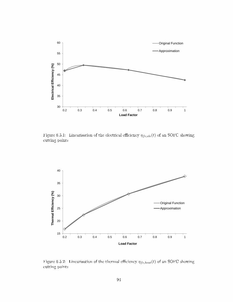
30
35
40
45
50
55
60
0.2 0.3 0.4 0.5 0.6 0.7 0.8 0.9 1
Ele
ctri
cal E
ffic
ien
cy (
%)
Load Factor
Original Function
Approximation
Figure 6.5.1: Linearisation of the electrical e�ciency ηfc,ele(t) of an SOFC showingcutting points
15
20
25
30
35
40
0.2 0.3 0.4 0.5 0.6 0.7 0.8 0.9 1
Th
erm
al E
ffic
ien
cy (
%)
Load Factor
Original Function
Approximation
Figure 6.5.2: Linearisation of the thermal e�ciency ηfc,heat(t) of an SOFC showingcutting points
94
Apart from the e�ciency equations, equation 6.4.1 is modi�ed:
Qfc,ele(t) = yfc(t) · Pfc ·3∑1
(yp(t) · rp(t)) (6.5.5)
and the following constraint has to be added:
3∑p=1
yp(t) = 1 (6.5.6)
The formulation of the model is still MINLP. Even though the e�ciency equations
have been linearised there are still equations in the model that non-linear. This step
was essential to simplify the model and to allow it to run.
6.6 Modelling Results
The presentation of the results for each dataset is divided in two cases: �rst, a design
without the option of a TST (Cases 1, 3, 5) and then a design with the storage tank
included (Cases 2, 4, 6).
6.6.1 Winter Day Analysis
6.6.1.1 Case 1
The values for the objective function and optimisation variables for the winter day
analysis are shown in Table 6.3. It can be seen from the table that the minimum CO2
emissions occur for a fuel cell capacity of 1.9 kWe and a boiler of 11.1 kWth. This
plant if operated as described below can result an approximate 7 % reduction in CO2
emissions from the reference building on a winter day. This system will be referred
to as �Case 1� in the analysis. The fuel cell capacity calculated is slightly higher
compared to similar studies in literature. Hawkes et al. calculated systems ranging
from 0.9 kWe to 1.3 kWe to provide a house with electricity and heat [73]. Many
studies on fuel cell micro-CHPs are carried out around the 1 kW value for electrical
capacity [14, 15, 18, 52]. However the value found here is still within the domestic
range for fuel cell capacities: Ang et al. mention that fuel cell systems in the range
of 1 to 10 kWe are suitable for dwellings [10]. Dodds et al. specify that domestic
fuel cell micro-CHPs are most widely used around the 1-3 kW thermal output [51].
This higher value can be related to the temporal precision which ignores operational
95
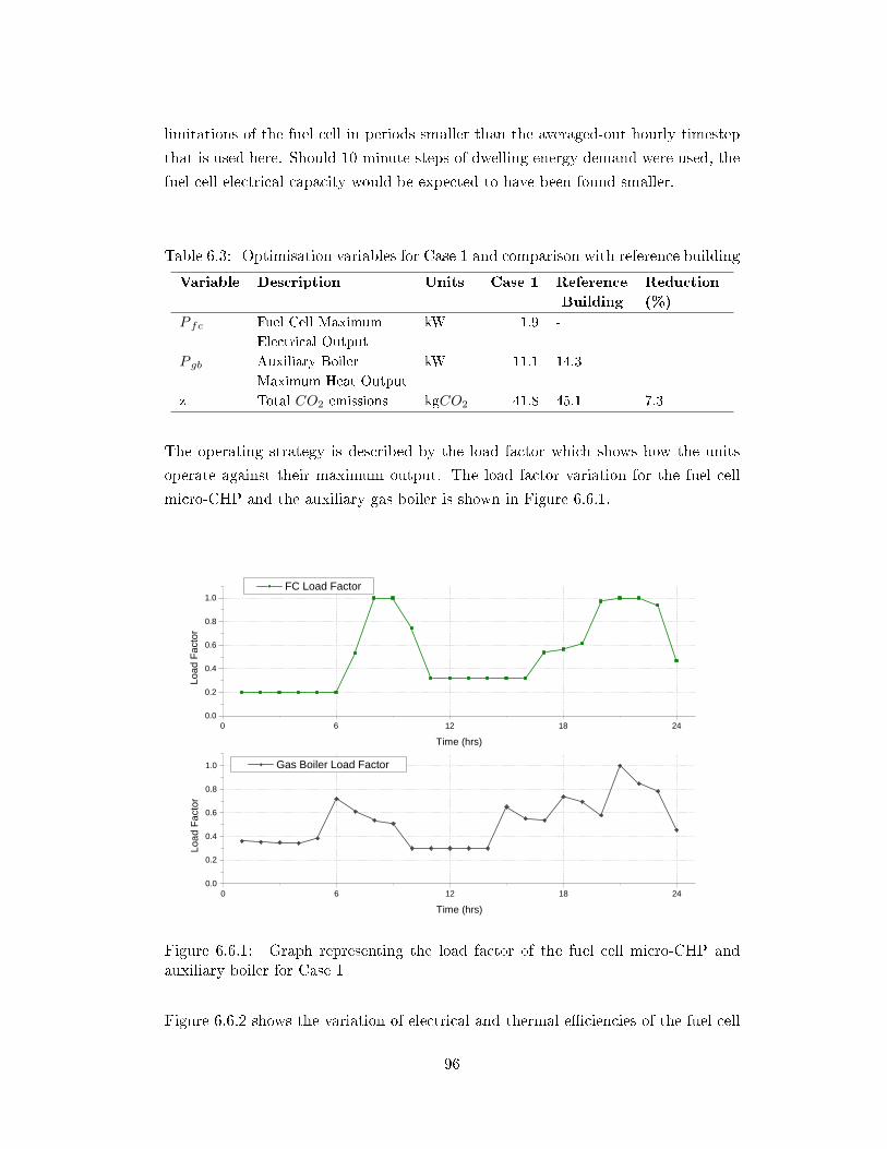
limitations of the fuel cell in periods smaller than the averaged-out hourly timestep
that is used here. Should 10-minute steps of dwelling energy demand were used, the
fuel cell electrical capacity would be expected to have been found smaller.
Table 6.3: Optimisation variables for Case 1 and comparison with reference building
Variable Description Units Case 1 Reference Reduction
Building (%)
P fc Fuel Cell Maximum kW 1.9 -
Electrical Output
P gb Auxiliary Boiler kW 11.1 14.3
Maximum Heat Output
z Total CO2 emissions kgCO2 41.8 45.1 7.3
The operating strategy is described by the load factor which shows how the units
operate against their maximum output. The load factor variation for the fuel cell
micro-CHP and the auxiliary gas boiler is shown in Figure 6.6.1.
0 6 1 2 1 8 2 40 . 0
0 . 2
0 . 4
0 . 6
0 . 8
1 . 0 F C L o a d F a c t o r
Load
Facto
r
T i m e ( h r s )
0 6 1 2 1 8 2 40 . 0
0 . 2
0 . 4
0 . 6
0 . 8
1 . 0
Load
Facto
r
T i m e ( h r s )
G a s B o i l e r L o a d F a c t o r
Figure 6.6.1: Graph representing the load factor of the fuel cell micro-CHP andauxiliary boiler for Case 1
Figure 6.6.2 shows the variation of electrical and thermal e�ciencies of the fuel cell
96
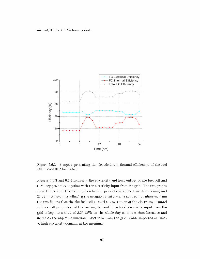
micro-CHP for the 24 hour period.
0 6 1 2 1 8 2 40
2 0
4 0
6 0
8 0
1 0 0
Efficie
ncy (
%)
T i m e ( h r s )
F C E l e c t r i c a l E f f i c i e n c y F C T h e r m a l E f f i c i e n c y T o t a l F C E f f i c i e n c y
Figure 6.6.2: Graph representing the electrical and thermal e�ciencies of the fuelcell micro-CHP for Case 1
Figures 6.6.3 and 6.6.4 represent the electricity and heat output of the fuel cell and
auxiliary gas boiler together with the electricity input from the grid. The two graphs
show that the fuel cell energy production peaks between 7-11 in the morning and
20-22 in the evening following the occupancy patterns. Also it can be observed from
the two �gures that the the fuel cell is sized to cover most of the electricity demand
and a small proportion of the heating demand. The total electricity input from the
grid is kept to a total of 2.25 kWh on the whole day as it is carbon intensive and
increases the objective function. Electricity from the grid is only imported at times
of high electricity demand in the morning.
97
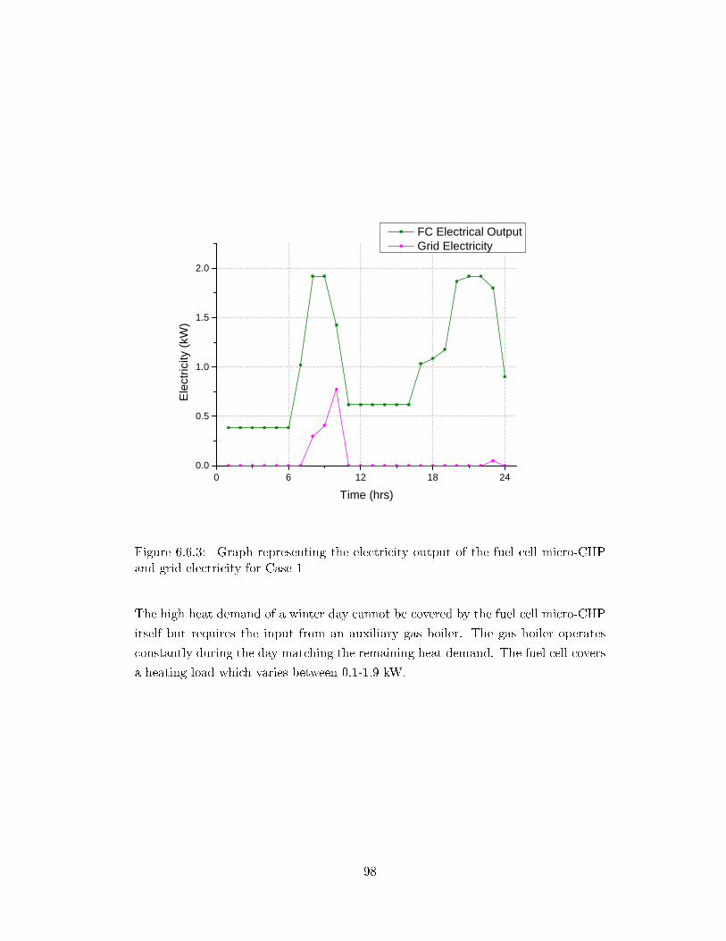
0 6 1 2 1 8 2 40 . 0
0 . 5
1 . 0
1 . 5
2 . 0
Electr
icity (
kW)
T i m e ( h r s )
F C E l e c t r i c a l O u t p u t G r i d E l e c t r i c i t y
Figure 6.6.3: Graph representing the electricity output of the fuel cell micro-CHPand grid electricity for Case 1
The high heat demand of a winter day cannot be covered by the fuel cell micro-CHP
itself but requires the input from an auxiliary gas boiler. The gas boiler operates
constantly during the day matching the remaining heat demand. The fuel cell covers
a heating load which varies between 0.1-1.9 kW.
98
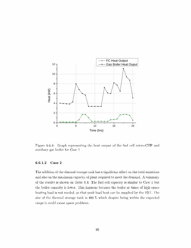
0 6 1 2 1 8 2 40
2
4
6
8
1 0
1 2
Heat
(kW)
T i m e ( h r s )
F C H e a t O u t p u t G a s B o i l e r H e a t O u p u t
Figure 6.6.4: Graph representing the heat output of the fuel cell micro-CHP andauxiliary gas boiler for Case 1
6.6.1.2 Case 2
The addition of the thermal storage tank has a signi�cant e�ect on the total emissions
and also on the maximum capacity of plant required to meet the demand. A summary
of the results is shown on Table 6.4. The fuel cell capacity is similar to Case 1 but
the boiler capacity is lower. This happens because the boiler at times of high space
heating load is not needed, as that peak load heat can be supplied by the TST. The
size of the thermal storage tank is 490 L which despite being within the expected
range it could cause space problems.
99
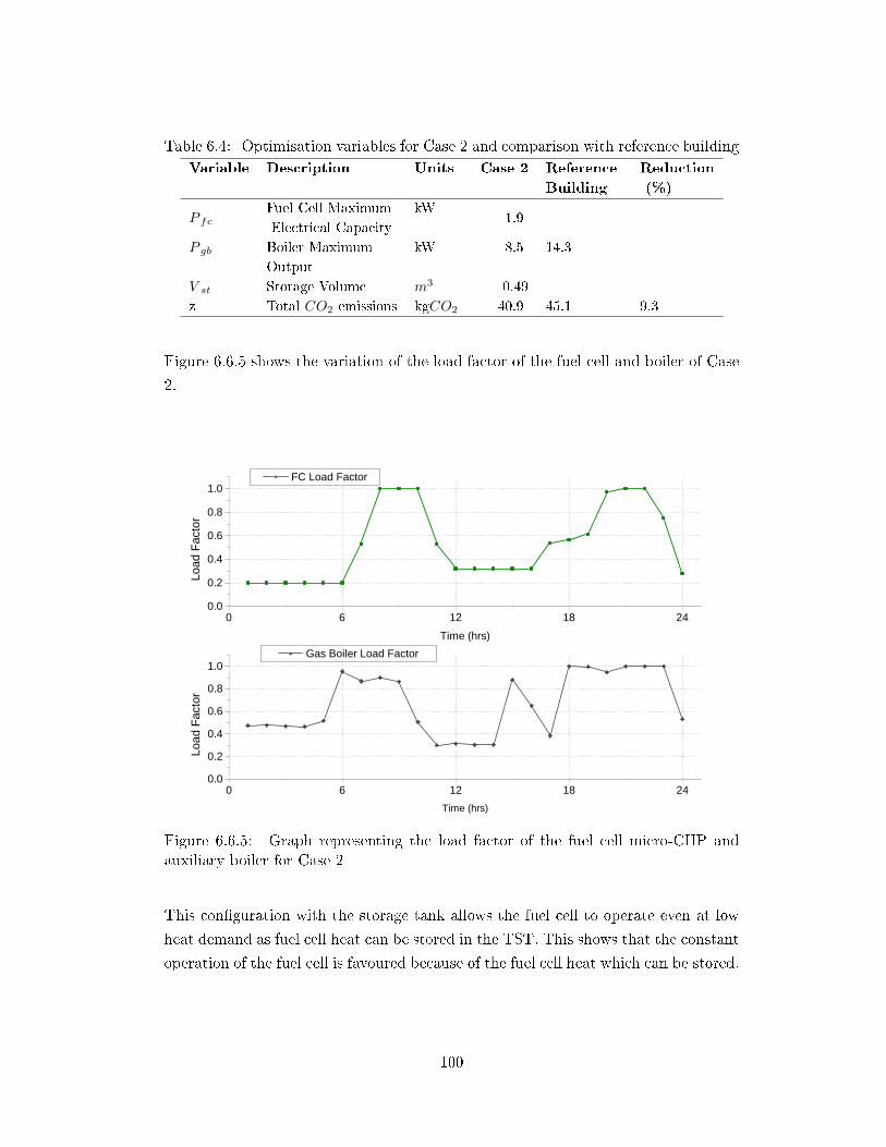
Table 6.4: Optimisation variables for Case 2 and comparison with reference buildingVariable Description Units Case 2 Reference Reduction
Building (%)
P fcFuel Cell Maximum kW
1.9Electrical Capacity
P gb Boiler Maximum kW 8.5 14.3
Output
V st Storage Volume m3 0.49
z Total CO2 emissions kgCO2 40.9 45.1 9.3
Figure 6.6.5 shows the variation of the load factor of the fuel cell and boiler of Case
2.
0 6 1 2 1 8 2 40 . 00 . 20 . 40 . 60 . 81 . 0
F C L o a d F a c t o r
Load
Facto
r
T i m e ( h r s )
0 6 1 2 1 8 2 40 . 00 . 20 . 40 . 60 . 81 . 0
G a s B o i l e r L o a d F a c t o r
Load
Facto
r
T i m e ( h r s )
Figure 6.6.5: Graph representing the load factor of the fuel cell micro-CHP andauxiliary boiler for Case 2
This con�guration with the storage tank allows the fuel cell to operate even at low
heat demand as fuel cell heat can be stored in the TST. This shows that the constant
operation of the fuel cell is favoured because of the fuel cell heat which can be stored.
100
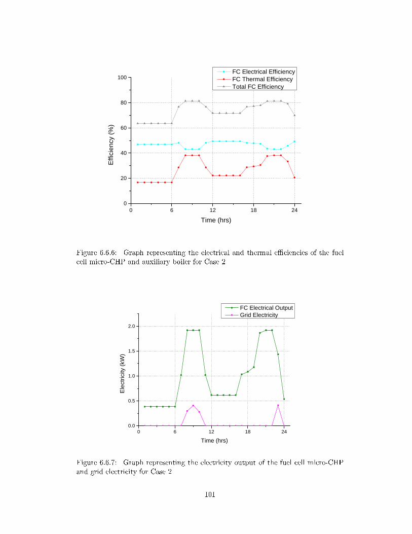
0 6 1 2 1 8 2 40
2 0
4 0
6 0
8 0
1 0 0
Efficie
ncy (
%)
T i m e ( h r s )
F C E l e c t r i c a l E f f i c i e n c y F C T h e r m a l E f f i c i e n c y T o t a l F C E f f i c i e n c y
Figure 6.6.6: Graph representing the electrical and thermal e�ciencies of the fuelcell micro-CHP and auxiliary boiler for Case 2
0 6 1 2 1 8 2 40 . 0
0 . 5
1 . 0
1 . 5
2 . 0
Electr
icity (
kW)
T i m e ( h r s )
F C E l e c t r i c a l O u t p u t G r i d E l e c t r i c i t y
Figure 6.6.7: Graph representing the electricity output of the fuel cell micro-CHPand grid electricity for Case 2
101
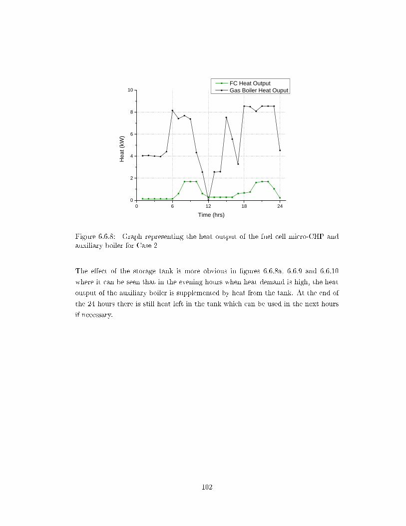
0 6 1 2 1 8 2 40
2
4
6
8
1 0
Heat
(kW)
T i m e ( h r s )
F C H e a t O u t p u t G a s B o i l e r H e a t O u p u t
Figure 6.6.8: Graph representing the heat output of the fuel cell micro-CHP andauxiliary boiler for Case 2
The e�ect of the storage tank is more obvious in �gures 6.6.8a, 6.6.9 and 6.6.10
where it can be seen that in the evening hours when heat demand is high, the heat
output of the auxiliary boiler is supplemented by heat from the tank. At the end of
the 24 hours there is still heat left in the tank which can be used in the next hours
if necessary.
102
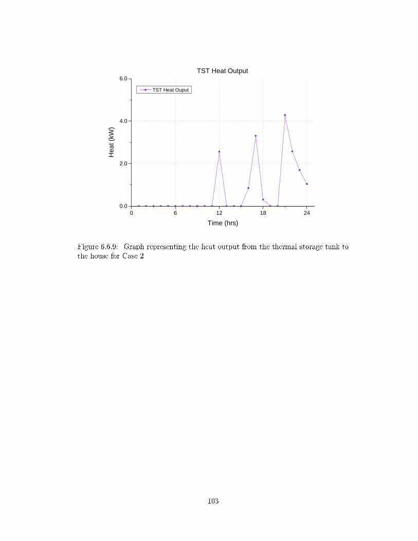
0 6 1 2 1 8 2 40 . 0
2 . 0
4 . 0
6 . 0 T S T H e a t O u p u t
T i m e ( h r s )
Heat
(kW)
T S T H e a t O u t p u t
Figure 6.6.9: Graph representing the heat output from the thermal storage tank tothe house for Case 2
103

0 6 1 2 1 8 2 40 . 0
2 . 0
4 . 0
6 . 0
8 . 0 T S T H e a t C o n t e n t
T i m e ( h r s )
Heat
(kWh)
T S T H e a t C o n t e n t
Figure 6.6.10: Graph representing the heat content of the thermal storage tankfor Case 2
6.6.2 Summer day analysis
6.6.2.1 Case 3
Optimisation for the summer day has di�erent results from the winter day. The
results are summarised in Table 6.5. The total percentage reduction in emissions
from the reference building is higher than in Case 1 and 2 and reaches approximately
22%. The optimisation variables also have di�erent values from the winter peak day:
the fuel cell is sized at a similar capacity as before and covers the electricity load
which has not changed from the winter operation. The gas boiler maximum output
has fallen down to 1 kW and serves the DHW load which cannot be covered entirely
by the fuel cell's heat output.
104
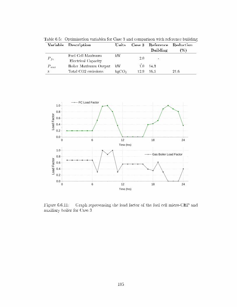
Table 6.5: Optimisation variables for Case 3 and comparison with reference buildingVariable Description Units Case 3 Reference Reduction
Building (%)
P fcFuel Cell Maximum kW
2.0 -Electrical Capacity
-P aux Boiler Maximum Output kW 1.0 14.3z Total CO2 emissions kgCO2 12.9 16.5 21.6
0 6 1 2 1 8 2 40 . 00 . 20 . 40 . 60 . 81 . 0
F C L o a d F a c t o r
Load
Facto
r
T i m e ( h r s )
0 6 1 2 1 8 2 40 . 00 . 20 . 40 . 60 . 81 . 0
G a s B o i l e r L o a d F a c t o r
Load
Facto
r
T i m e ( h r s )
Figure 6.6.11: Graph representing the load factor of the fuel cell micro-CHP andauxiliary boiler for Case 3
105
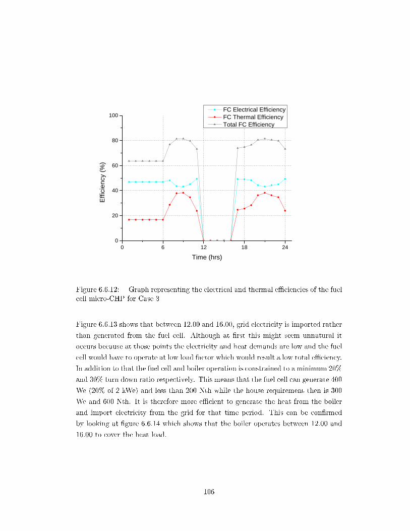
0 6 1 2 1 8 2 40
2 0
4 0
6 0
8 0
1 0 0Eff
icienc
y (%)
T i m e ( h r s )
F C E l e c t r i c a l E f f i c i e n c y F C T h e r m a l E f f i c i e n c y T o t a l F C E f f i c i e n c y
Figure 6.6.12: Graph representing the electrical and thermal e�ciencies of the fuelcell micro-CHP for Case 3
Figure 6.6.13 shows that between 12.00 and 16.00, grid electricity is imported rather
than generated from the fuel cell. Although at �rst this might seem unnatural it
occurs because at those points the electricity and heat demands are low and the fuel
cell would have to operate at low load factor which would result a low total e�ciency.
In addition to that the fuel cell and boiler operation is constrained to a minimum 20%
and 30% turn down ratio respectively. This means that the fuel cell can generate 400
We (20% of 2 kWe) and less than 200 Nth while the house requirement then is 300
We and 600 Nth. It is therefore more e�cient to generate the heat from the boiler
and import electricity from the grid for that time period. This can be con�rmed
by looking at �gure 6.6.14 which shows that the boiler operates between 12.00 and
16.00 to cover the heat load.
106
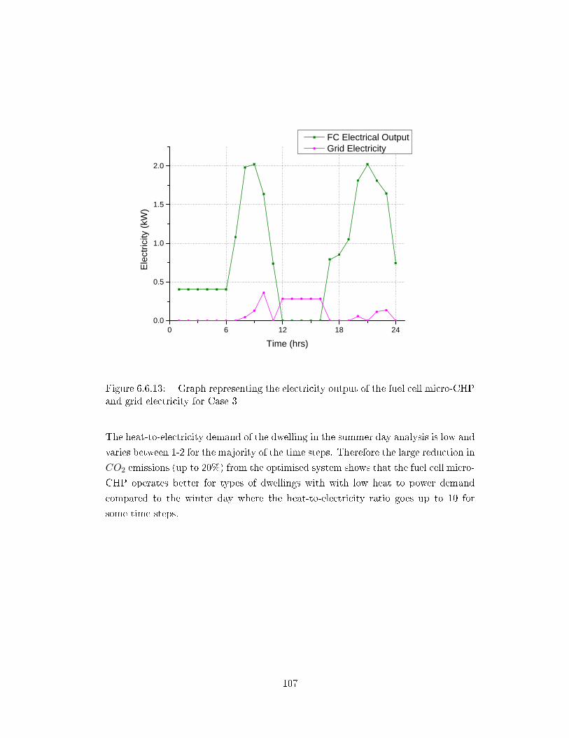
0 6 1 2 1 8 2 40 . 0
0 . 5
1 . 0
1 . 5
2 . 0
Electr
icity (
kW)
T i m e ( h r s )
F C E l e c t r i c a l O u t p u t G r i d E l e c t r i c i t y
Figure 6.6.13: Graph representing the electricity output of the fuel cell micro-CHPand grid electricity for Case 3
The heat-to-electricity demand of the dwelling in the summer day analysis is low and
varies between 1-2 for the majority of the time steps. Therefore the large reduction in
CO2 emissions (up to 20%) from the optimised system shows that the fuel cell micro-
CHP operates better for types of dwellings with with low heat to power demand
compared to the winter day where the heat-to-electricity ratio goes up to 10 for
some time steps.
107
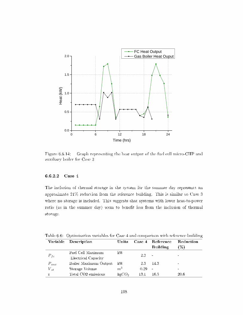
0 6 1 2 1 8 2 40 . 0
0 . 5
1 . 0
1 . 5
2 . 0He
at (kW
)
T i m e ( h r s )
F C H e a t O u t p u t G a s B o i l e r H e a t O u p u t
Figure 6.6.14: Graph representing the heat output of the fuel cell micro-CHP andauxiliary boiler for Case 3
6.6.2.2 Case 4
The inclusion of thermal storage in the system for the summer day represents an
approximate 21% reduction from the reference building. This is similar to Case 3
where no storage is included. This suggests that systems with lower heat-to-power
ratio (as in the summer day) seem to bene�t less from the inclusion of thermal
storage.
Table 6.6: Optimisation variables for Case 4 and comparison with reference buildingVariable Description Units Case 4 Reference Reduction
Building (%)
P fcFuel Cell Maximum kW
2.2 - -Electrical Capacity
P aux Boiler Maximum Output kW 2.3 14.3 -
V st Storage Volume m3 0.29 - -
z Total CO2 emissions kgCO2 13.1 16.5 20.6
108

The capacity of the auxiliary boiler is decreased from Case 2 from 8.5 to 2.3 kW but
the capacity of the fuel cell is similar (from 1.9 kW to 2.2 kW). There is no gas boiler
product rated at 2.3 kW and this number is only indicative of the capacities needed
to satisfy demand.
0 6 1 2 1 8 2 40 . 00 . 20 . 40 . 60 . 81 . 0
F C L o a d F a c t o r
Load
Facto
r
T i m e ( h r s )
0 6 1 2 1 8 2 40 . 00 . 20 . 40 . 60 . 81 . 0
G a s B o i l e r L o a d F a c t o r
Load
Facto
r
T i m e ( h r s )
Figure 6.6.15: Graph representing the load factor of the fuel cell micro-CHP andauxiliary boiler for Case 4
The size of the storage tank in this scenario is 290 L which lies within the availability
limits of products. The e�ect of the storage tank in the summer scenario does not
seem to bene�t the reduction of CO2 emissions compared to Case 3.
109
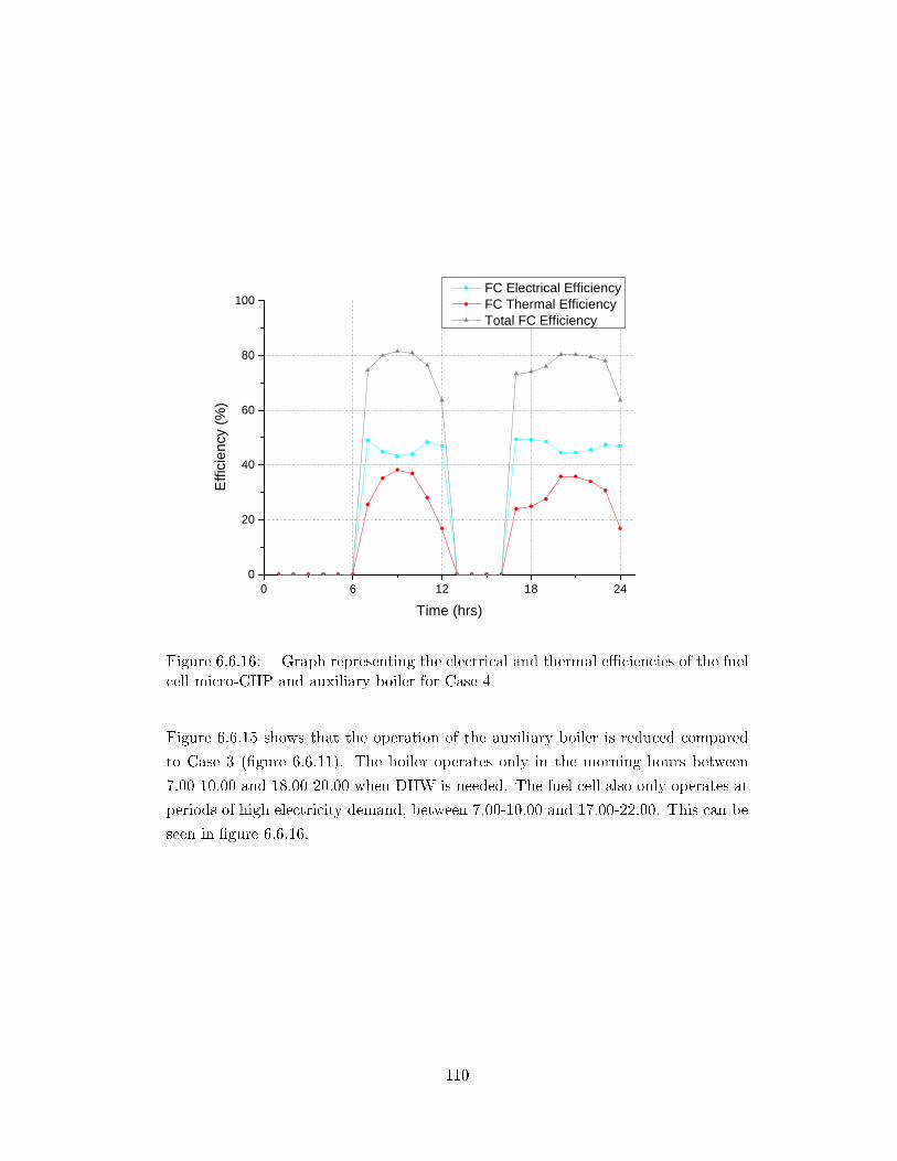
0 6 1 2 1 8 2 40
2 0
4 0
6 0
8 0
1 0 0
Efficie
ncy (
%)
T i m e ( h r s )
F C E l e c t r i c a l E f f i c i e n c y F C T h e r m a l E f f i c i e n c y T o t a l F C E f f i c i e n c y
Figure 6.6.16: Graph representing the electrical and thermal e�ciencies of the fuelcell micro-CHP and auxiliary boiler for Case 4
Figure 6.6.15 shows that the operation of the auxiliary boiler is reduced compared
to Case 3 (�gure 6.6.11). The boiler operates only in the morning hours between
7.00-10.00 and 18.00-20.00 when DHW is needed. The fuel cell also only operates at
periods of high electricity demand, between 7.00-10.00 and 17.00-22.00. This can be
seen in �gure 6.6.16.
110
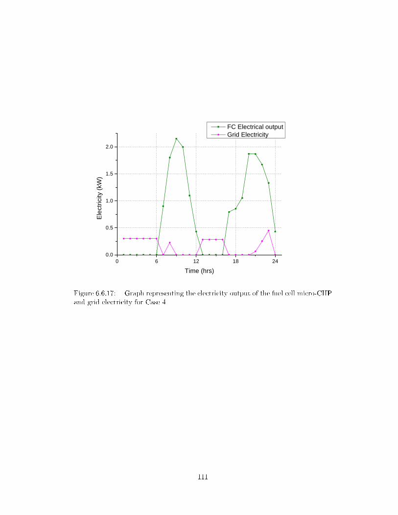
0 6 1 2 1 8 2 40 . 0
0 . 5
1 . 0
1 . 5
2 . 0
Electr
icity (
kW)
T i m e ( h r s )
F C E l e c t r i c a l o u t p u t G r i d E l e c t r i c i t y
Figure 6.6.17: Graph representing the electricity output of the fuel cell micro-CHPand grid electricity for Case 4
111
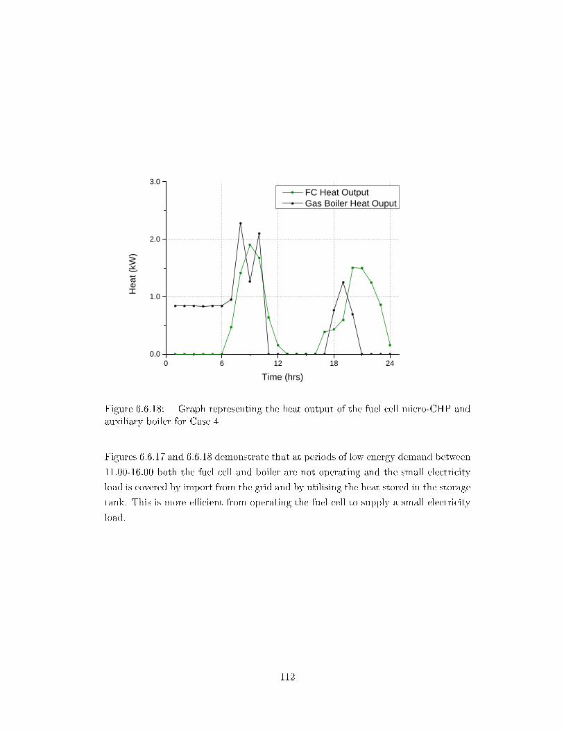
0 6 1 2 1 8 2 40 . 0
1 . 0
2 . 0
3 . 0
Heat
(kW)
T i m e ( h r s )
F C H e a t O u t p u t G a s B o i l e r H e a t O u p u t
Figure 6.6.18: Graph representing the heat output of the fuel cell micro-CHP andauxiliary boiler for Case 4
Figures 6.6.17 and 6.6.18 demonstrate that at periods of low energy demand between
11.00-16.00 both the fuel cell and boiler are not operating and the small electricity
load is covered by import from the grid and by utilising the heat stored in the storage
tank. This is more e�cient from operating the fuel cell to supply a small electricity
load.
112

0 6 1 2 1 8 2 40 . 0
2 . 0
4 . 0 T S T H e a t O u p u t
T i m e ( h r s )
Heat
(kW)
T S T H e a t O u t p u t
Figure 6.6.19: Graph representing the heat output from the thermal storage tankto the house for Case 4
113
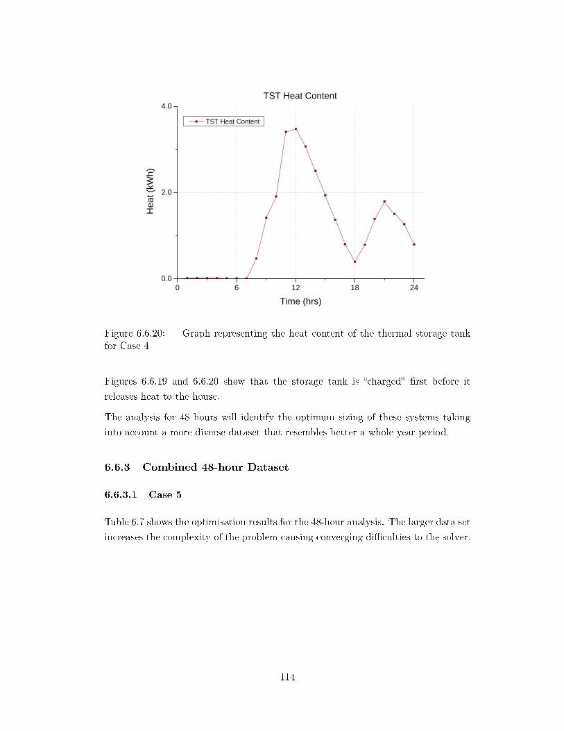
0 6 1 2 1 8 2 40 . 0
2 . 0
4 . 0 T S T H e a t C o n t e n t
T i m e ( h r s )
Heat
(kWh)
T S T H e a t C o n t e n t
Figure 6.6.20: Graph representing the heat content of the thermal storage tankfor Case 4
Figures 6.6.19 and 6.6.20 show that the storage tank is �charged� �rst before it
releases heat to the house.
The analysis for 48 hours will identify the optimum sizing of these systems taking
into account a more diverse dataset that resembles better a whole year period.
6.6.3 Combined 48-hour Dataset
6.6.3.1 Case 5
Table 6.7 shows the optimisation results for the 48-hour analysis. The larger data set
increases the complexity of the problem causing converging di�culties to the solver.
114
Table 6.7: Optimisation variables for Case 5 and comparison with reference buildingVariable Description Units Case 5 Reference Reduction
Building (%)
P fcFuel Cell Maximum kW
2.0 - -Electrical Capacity
P aux Boiler Maximum Output kW 11.0 14.3 -
z Total CO2 emissions kgCO2 61.2 61.5 0.05
The design proposed in Case 5 cannot o�er any reduction in CO2 emissions from the
reference building. This is caused by the gas boiler which is sized to cover both the
winter and summer load and its 30% minimum turn down ratio. Sizing the boiler
for the winter load ensures that heat demand would be covered at all times but it
creates an issue in the summer. The boiler's minimum heat output in some timesteps
exceeds the low summer heat demand and this unused heat causes the additional
CO2 emissions. This is demonstrated for the summer period in �gures 6.6.21 and
6.6.24. This suggests that this con�guration might not be ideal for primary energy
consumption reduction. The addition of a storage tank between the load and the
fuel cell should enable the fuel cell to operate more hours and reduce the operation
of the boiler. This case will be examined next.
A solution was also obtained for a lower 25% limit for the turn down of the boiler
and the resulting CO2 emissions were reduced to 60.6 kgCo2, con�rming the point
made above.
115
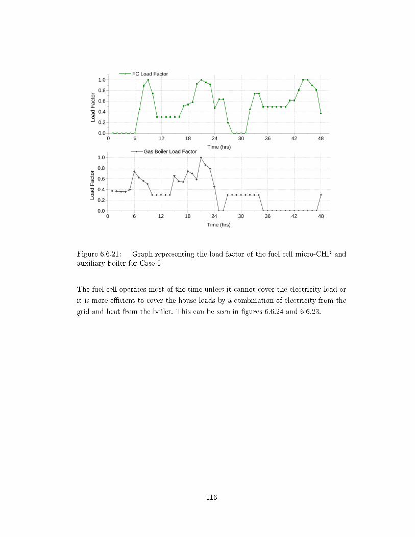
0 6 1 2 1 8 2 4 3 0 3 6 4 2 4 80 . 00 . 20 . 40 . 60 . 81 . 0
F C L o a d F a c t o r
Load
Facto
r
T i m e ( h r s )
0 6 1 2 1 8 2 4 3 0 3 6 4 2 4 80 . 00 . 20 . 40 . 60 . 81 . 0
G a s B o i l e r L o a d F a c t o r
Load
Facto
r
T i m e ( h r s )
Figure 6.6.21: Graph representing the load factor of the fuel cell micro-CHP andauxiliary boiler for Case 5
The fuel cell operates most of the time unless it cannot cover the electricity load or
it is more e�cient to cover the house loads by a combination of electricity from the
grid and heat from the boiler. This can be seen in �gures 6.6.24 and 6.6.23.
116
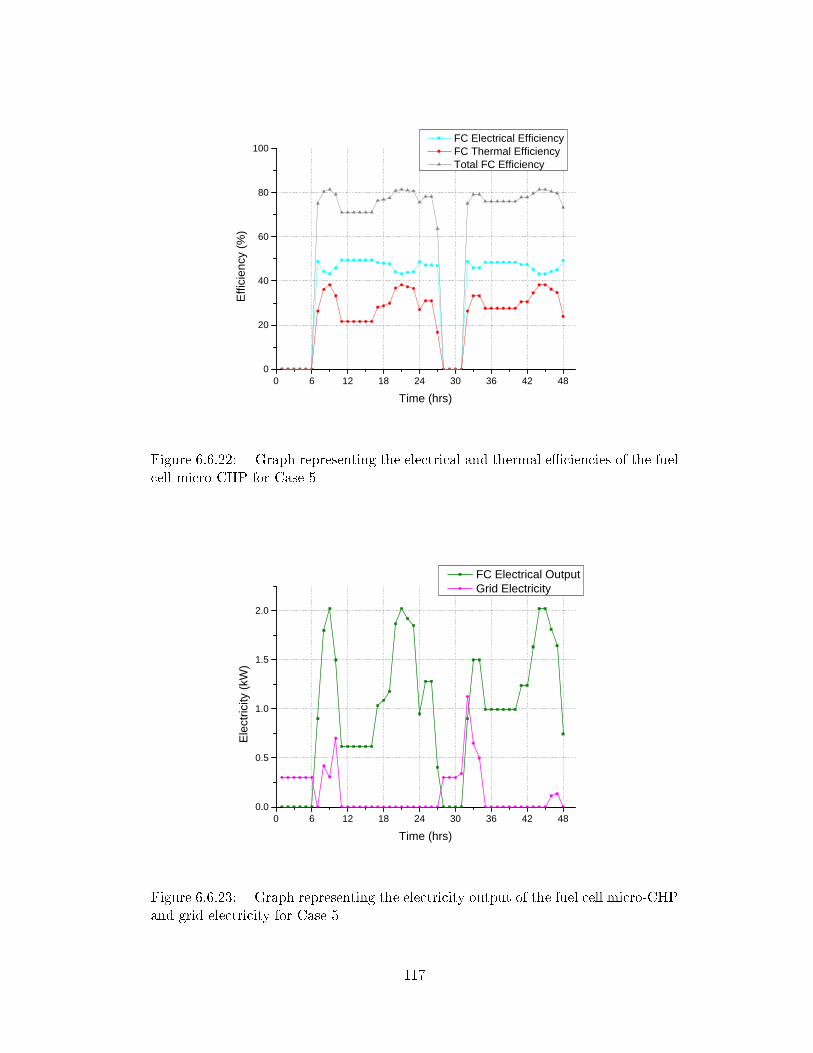
0 6 1 2 1 8 2 4 3 0 3 6 4 2 4 80
2 0
4 0
6 0
8 0
1 0 0
Efficie
ncy (
%)
T i m e ( h r s )
F C E l e c t r i c a l E f f i c i e n c y F C T h e r m a l E f f i c i e n c y T o t a l F C E f f i c i e n c y
Figure 6.6.22: Graph representing the electrical and thermal e�ciencies of the fuelcell micro-CHP for Case 5
0 6 1 2 1 8 2 4 3 0 3 6 4 2 4 80 . 0
0 . 5
1 . 0
1 . 5
2 . 0
Electr
icity (
kW)
T i m e ( h r s )
F C E l e c t r i c a l O u t p u t G r i d E l e c t r i c i t y
Figure 6.6.23: Graph representing the electricity output of the fuel cell micro-CHPand grid electricity for Case 5
117
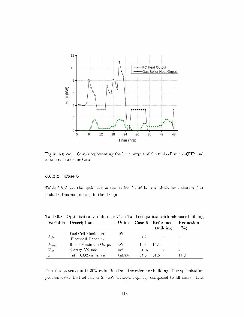
0 6 1 2 1 8 2 4 3 0 3 6 4 2 4 80
2
4
6
8
1 0
1 2
Heat
(kW)
T i m e ( h r s )
F C H e a t O u t p u t G a s B o i l e r H e a t O u p u t
Figure 6.6.24: Graph representing the heat output of the fuel cell micro-CHP andauxiliary boiler for Case 5
6.6.3.2 Case 6
Table 6.8 shows the optimisation results for the 48 hour analysis for a system that
includes thermal storage in the design.
Table 6.8: Optimisation variables for Case 6 and comparison with reference buildingVariable Description Units Case 6 Reference Reduction
Building (%)
P fcFuel Cell Maximum kW
2.5 - -Electrical Capacity
-P aux Boiler Maximum Output kW 10.3 14.3 -
V st Storage Volume m3 0.76 - -
z Total CO2 emissions kgCO2 54.6 61.5 11.3
Case 6 represents an 11.30% reduction from the reference building. The optimisation
process sized the fuel cell at 2.5 kW a larger capacity compared to all cases. This
118
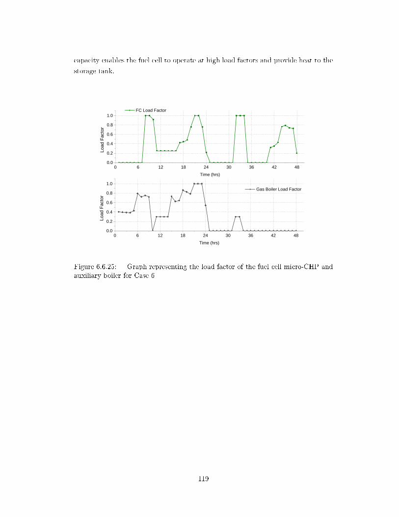
capacity enables the fuel cell to operate at high load factors and provide heat to the
storage tank.
0 6 1 2 1 8 2 4 3 0 3 6 4 2 4 80 . 00 . 20 . 40 . 60 . 81 . 0
F C L o a d F a c t o rLo
ad Fa
ctor
T i m e ( h r s )
0 6 1 2 1 8 2 4 3 0 3 6 4 2 4 80 . 00 . 20 . 40 . 60 . 81 . 0
G a s B o i l e r L o a d F a c t o r
Load
Facto
r
T i m e ( h r s )
Figure 6.6.25: Graph representing the load factor of the fuel cell micro-CHP andauxiliary boiler for Case 6
119
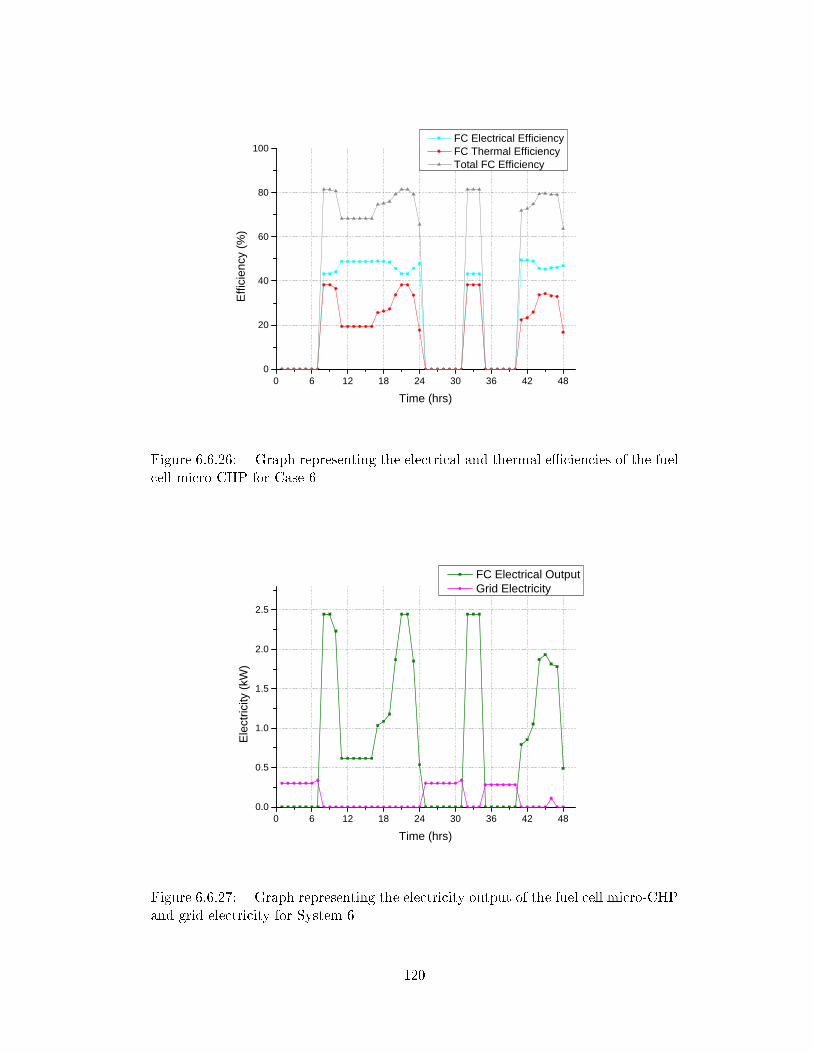
0 6 1 2 1 8 2 4 3 0 3 6 4 2 4 80
2 0
4 0
6 0
8 0
1 0 0
Efficie
ncy (
%)
T i m e ( h r s )
F C E l e c t r i c a l E f f i c i e n c y F C T h e r m a l E f f i c i e n c y T o t a l F C E f f i c i e n c y
Figure 6.6.26: Graph representing the electrical and thermal e�ciencies of the fuelcell micro-CHP for Case 6
0 6 1 2 1 8 2 4 3 0 3 6 4 2 4 80 . 0
0 . 5
1 . 0
1 . 5
2 . 0
2 . 5
Electr
icity (
kW)
T i m e ( h r s )
F C E l e c t r i c a l O u t p u t G r i d E l e c t r i c i t y
Figure 6.6.27: Graph representing the electricity output of the fuel cell micro-CHPand grid electricity for System 6
120
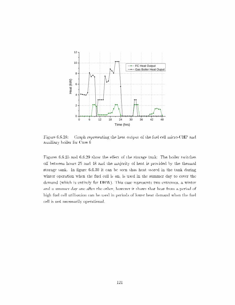
0 6 1 2 1 8 2 4 3 0 3 6 4 2 4 80
2
4
6
8
1 0
1 2
Heat
(kW)
T i m e ( h r s )
F C H e a t O u t p u t G a s B o i l e r H e a t O u p u t
Figure 6.6.28: Graph representing the heat output of the fuel cell micro-CHP andauxiliary boiler for Case 6
Figures 6.6.25 and 6.6.29 show the e�ect of the storage tank: The boiler switches
o� between hours 25 and 48 and the majority of heat is provided by the thermal
storage tank. In �gure 6.6.30 it can be seen that heat stored in the tank during
winter operation when the fuel cell is on, is used in the summer day to cover the
demand (which is entirely for DHW). This case represents two extremes, a winter
and a summer day one after the other, however it shows that heat from a period of
high fuel cell utilisation can be used in periods of lower heat demand when the fuel
cell is not necessarily operational.
121
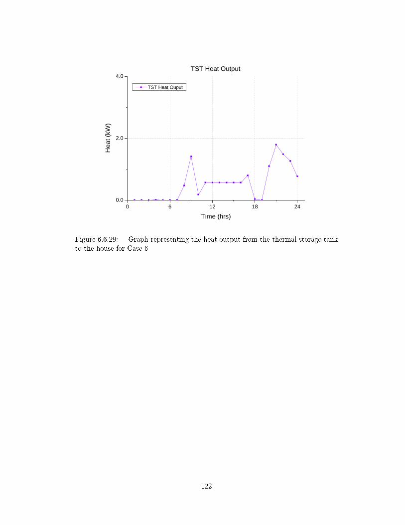
0 6 1 2 1 8 2 40 . 0
2 . 0
4 . 0 T S T H e a t O u p u t
T i m e ( h r s )
Heat
(kW)
T S T H e a t O u t p u t
Figure 6.6.29: Graph representing the heat output from the thermal storage tankto the house for Case 6
122
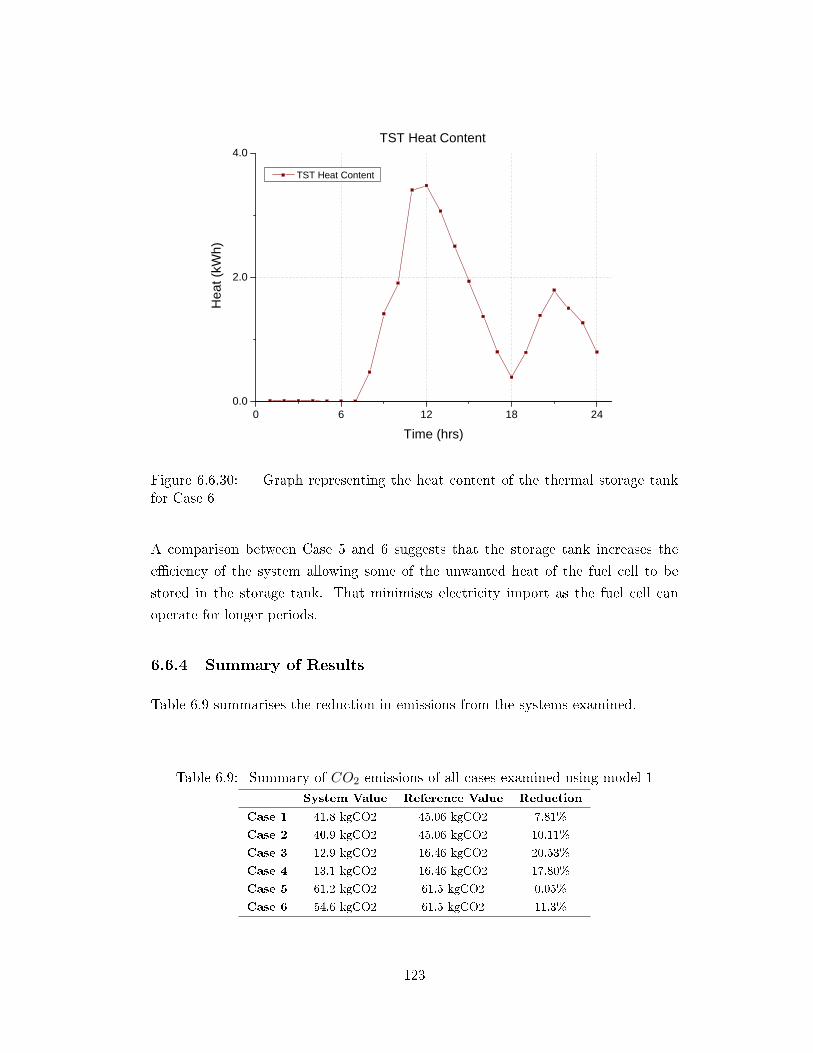
0 6 1 2 1 8 2 40 . 0
2 . 0
4 . 0 T S T H e a t C o n t e n t
T i m e ( h r s )
Heat
(kWh)
T S T H e a t C o n t e n t
Figure 6.6.30: Graph representing the heat content of the thermal storage tankfor Case 6
A comparison between Case 5 and 6 suggests that the storage tank increases the
e�ciency of the system allowing some of the unwanted heat of the fuel cell to be
stored in the storage tank. That minimises electricity import as the fuel cell can
operate for longer periods.
6.6.4 Summary of Results
Table 6.9 summarises the reduction in emissions from the systems examined.
Table 6.9: Summary of CO2 emissions of all cases examined using model 1System Value Reference Value Reduction
Case 1 41.8 kgCO2 45.06 kgCO2 7.81%
Case 2 40.9 kgCO2 45.06 kgCO2 10.11%
Case 3 12.9 kgCO2 16.46 kgCO2 20.53%
Case 4 13.1 kgCO2 16.46 kgCO2 17.80%
Case 5 61.2 kgCO2 61.5 kgCO2 0.05%
Case 6 54.6 kgCO2 61.5 kgCO2 11.3%
123
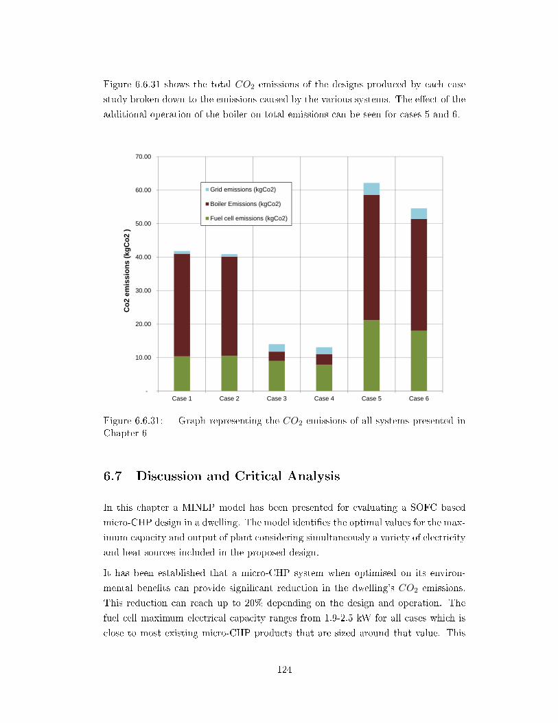
Figure 6.6.31 shows the total CO2 emissions of the designs produced by each case
study broken down to the emissions caused by the various systems. The e�ect of the
additional operation of the boiler on total emissions can be seen for cases 5 and 6.
-
10.00
20.00
30.00
40.00
50.00
60.00
70.00
Case 1 Case 2 Case 3 Case 4 Case 5 Case 6
Co
2 em
issi
on
s (k
gC
o2
)
Grid emissions (kgCo2)
Boiler Emissions (kgCo2)
Fuel cell emissions (kgCo2)
Figure 6.6.31: Graph representing the CO2 emissions of all systems presented inChapter 6
6.7 Discussion and Critical Analysis
In this chapter a MINLP model has been presented for evaluating a SOFC based
micro-CHP design in a dwelling. The model identi�es the optimal values for the max-
imum capacity and output of plant considering simultaneously a variety of electricity
and heat sources included in the proposed design.
It has been established that a micro-CHP system when optimised on its environ-
mental bene�ts can provide signi�cant reduction in the dwelling's CO2 emissions.
This reduction can reach up to 20% depending on the design and operation. The
fuel cell maximum electrical capacity ranges from 1.9-2.5 kW for all cases which is
close to most existing micro-CHP products that are sized around that value. This
124
provides some indirect validation of the results from the industry, as the fuel cell
based micro-CHP products are at the 1-3 kW capacity.
A TST can increase the energy availability of the system and reduce peaks of heat
demand in winter. Including a TST in the design, allows for reduced sizing of plant
as it was the case with the gas boiler in the winter day case studies. The boiler's
capacity dropped from 11 kW to 8.5 kW while at the same time the hours of operation
also dropped. The fuel cell system achieved longer operation and higher reductions
in CO2 emissions when storage was available. The TST allows the fuel cell micro-
CHP to cover the majority of the electricity demand and to minimise electricity
import from the electricity grid even when there is no heat demand by storing the
recovered heat in the thermal storage tank. The e�ect of the TST on CO2 emissions
reduction is greater in winter than in summer. The 48 hour analysis that includes
a more complete data set with winter and summer days, showed that a thermal
storage tank is essential for the system to provide emissions reduction. The sizing of
the boiler to cover the winter load and its operational turn down constraints cause
the system to produce some additional CO2 emissions.
The results showed that the fuel cell in some cases starts and stops twice during the
examined periods (case 4, case 5, case 6). SOFCs operate at high temperatures so
when an SOFC cools down to the environmental temperature it stresses the stack
materials and results in degradation of the components [107]. Also, it would take
some time for it to warm up again to 700 oC-100 oC [108] and restart producing
electricity. The operation of SOFCs micro-CHPs fuelled by natural gas is depend-
ent on the su�ciency of heat provided by the fuel cell to the reformer to maintain
the steam reforming reaction. On start up however, when heat from the fuel cell is
not available, the reformer is designed to operate on partial oxidation which is an
exothermic reaction. Partial oxidation and steam reforming occur combined at the
reformer from low output to full output operation [108]. Recent research is focused
on lowering SOFC operating temperatures in order to reduce thermal stress and in-
crease start-up times. Alvarez et al. studied the optimisation of a hybrid start-up
process of an intermediate temperature SOFC, showing that a start-up time of 286
s can be achieved [105]. In terms of thermal management an option is to seal with
insulating materials the SOFC stack and keep it within the operating temperature
of the stack. Apfel et al. showed that using Microtherm, a low-conductivity ma-
terial, the cool down period can be extended to days [11]. Providing an e�ective
thermal management strategy for SOFC based micro-CHPs becomes essential to re-
duce thermal cycles as the number of total start-up cycles of SOFC systems should
be below 100 [11]. Therefore, the results that allow the fuel cell to turn on and o�
125
twice during a 24-hour period are still achievable as long as the stack temperature
does not drop below the operating points. In terms of the system design the manu-
facturers would be forced to seal the stack with an advanced insulating material to
allow for this type of thermal management to occur and prevent stack degradation.
Fuel cell micro-CHPs perform better in dwellings with lower heat than electricity
demands due to their low heat-to-power ratio. This was demonstrated in this study
as higher reductions occur at the summer case studies that heat and electricity
demand are in the same order. This can be seen in table 6.9.
The methodology used in the presented work although subject to limitations (see
6.8) is a new approach in modelling micro-CHP fuel cell systems in dwellings. It
considers the variability of the energy patterns of the dwelling which are produced
in BIM software and the interaction with the fuel cell and its operation. It is not a
technique that only maximises the fuel cell's e�ciency which might not be the op-
timum choice for the overall CO2 emissions of the system but considers the variation
of the dwelling's energy demand.
The results obtained by using the 48 hour data set give an approximation of how
the system would perform on a yearly basis, however a bigger data set would give
more representative results. This is the approach followed in the analysis presented
in chapter 7.
Allowing any data set (real or from building simulation) to be used in the model as
input the �exibility of the process increases. This methodology is also very adapt-
able to adding other technologies as the models for all plant are based on e�ciency
equations.
6.8 Limitations of the study
This study has identi�ed some fundamental points in the design and operation of fuel
cell micro-CHPs and their interaction with the varying energy demands of a house.
It has limitations as its goal is to provide a reliable tool that can be used in the
early stages of the design. It is therefore not providing the actual design. The model
as it has been formulated does not provide information on how the various items
of plant are connected to each other but examines predetermined con�gurations.
In addition there is no indication of system �ows and temperatures. The inclusion
of temperature and �ow rates information for the di�erent process streams within
the fuel cell micro-CHP and the dwelling's space heating and DHW circuits could
provide a complete design solution. This solution could provide information on how
126
each stream of heat within the fuel cell process can be used more e�ectively for the
dwelling processes.
The results obtained for thermal storage systems assume that there is no heat loss
to the surroundings. A model that would consider storage losses would result in
a system that relies less on heat storage by reducing the amount of heat that gets
stored in the tank. A priority would be introduced for a quick release of heat from
the tank to increase e�ciency as possible and reduce losses.
Another weakness of this model has to do with the hourly timesteps which a�ect the
environmental results of the model. This however, is a weakness that is di�cult to
overcome when working on optimisation models that attempt to capture a whole year
period. This is because increasing temporal precision will result in more complex
models that are di�cult to solve.
6.9 Concluding Remarks
This study has presented a micro-CHP model of a dwelling that could be used in an
environmental bene�t analysis. The model considers di�erent options for satisfying
the energy demand of a UK dwelling. Data sets for di�erent scenarios were produced
using BIM software and were used to determine sizing characteristics and operational
pro�les of all plant involved in a design based around a fuel cell micro-CHP system.
Thermal energy storage was included in the model in addition to a gas boiler anda fuel
cell micro-CHP. It was established that fuel cell based micro-CHP systems perform
better in houses with similar electricity and heat loads. The design that produced
the best results on a combined winter-summer dataset, was a fuel cell micro-CHP
system coupled with a thermal energy storage tank . This combination enabled the
fuel cell micro-CHP to store heat in the thermal tank when heat demand was low,
so it could be used later, thus reducing the dependence on the auxiliary boiler. The
results also identi�ed a design requirement for SOFC based micro-CHP products
which is the need for high quality insulation on the stack to prevent the temperature
to drop below the operating temperature. Implementation of such measures could
prevent thermal cycling and increase lifetime.
127
Chapter 7
Model 2 - An MINLP model for
PEMFC based micro-CHP design
in dwellings
In this chapter, an innovative methodology based around the principles of mathem-
atical programming is proposed for the design of fuel cell micro-CHPs in dwellings.
This is presented along with the fundamental basics of the model and the solution
approach utilised. This study is motivated by the missing elements identi�ed in the
limitations of the previous model but also in the literature review which is a link
between the heat sources and demand.
7.1 Problem Statement
The overall problem for the design of a micro-CHP in a dwelling can be stated as
follows.
Given:
� A selection of heat an electricity generating plant;
� The heat and electricity demand for a dwelling;
� A low temperature hot water (LTHW ) pipework network to deliver the heat
demand;
� Process limitations and constraints in terms of energy generation and temper-
ature in pipes.
128
Determine:
� The con�guration and design between heat and electricity plant and consump-
tion within the dwelling.
� The sizing and operational characteristics of this design.
So as to optimise the resulting CO2 emissions from the whole dwelling energy system.
7.2 Basis for the PEMFC Model
PEMFC-based micro-CHPs deliver recoverable heat at the exit of the afterburner
and at the cooling circuit of the cell. The various heat and power generation units
and their interconnections in�uence the design and operation of the system and
determine how energy demand is met. Residential energy demand varies daily and
seasonally while the heat generation plant that can be used in a fuel cell micro-CHP
design also has variability in temperature and operating point. Constraints related
to temperatures and operational pro�les imposed by heating sources and demands
, should be balanced to provide a better dwelling design. As multiple heat streams
exist within a fuel cell micro-CHP system and considering that they have to be
integrated into the building heating services suggest that a systematic design tool
can be used to improve the design of fuel cell micro-CHPs in dwellings by providing
better utilisation of heat. This study presents this systematic tool which is based on
an optimisation framework.
7.3 Modelling Methodology
The basic components of the model that has been implemented can be seen in Figure
7.3.1. The main points used for the model are the following:
� The fuel cell generates electricity and heat consumingH2 reformed from natural
gas in the external reformer.
� The heat required for reforming is recovered from the afterburner stream.
� Heat from the fuel cell micro-CHP unit that can be used in the dwelling is
recovered by the cooling system of the fuel cell and from the afterburner exhaust
stream.
129
� A natural gas boiler supplements the heat recovered by the fuel cell stack and
afterburner to satisfy heat demand of the dwelling.
� The electricity grid supplements the electricity generated by the fuel cell to
satisfy the power demand of the dwelling.
� All heat recovered from the fuel cell processes and generated by the boiler can
be used in separate space heating and domestic hot water circuits via a low
temperature hot water circuit.
� Α thermal storage tank can store heat from either fuel cell heat sources.
� There are two low loss headers that serve heating and domestic hot water tank.
Heat from all sources via the two headers serve space heating and DHW tank.
The main assumptions made in the model are:
� Natural gas used in the system is assumed to be pure CH4.
� There is atmospheric pressure on the fuel cell processes.
� There are no heat losses or thermal strati�cation included in the TST model.
130
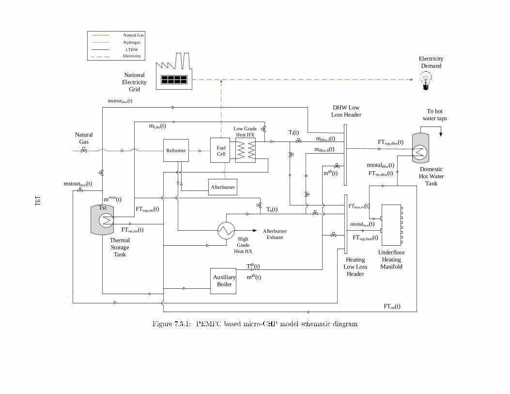
Domestic Hot Water
Tank
Underfloor Heating
Manifold
DHW Low Loss Header
Heating Low Loss
Header
To hot water taps
Fuel Cell
Afterburner Exhaust
Auxiliary Boiler
Thermal Storage Tank
ml,sto(t)
mstout(t)
mstoutheat(t)
High Grade
Heat HX
Low Grade Heat HX
FTret(t)
mtotaldhw(t)FTret,dhw(t)
FTsup,dhw(t)
FTsup,heat(t)
Tgb(t)
mgb(t)
mdhw,l(t)
mgb(t)
Tl(t)
Th(t)
Reformer
Afterburner
Natural Gas
Electricity Demand
National Electricity
Grid
Natural Gas
Hydrogen
Electricity
LTHW
Tst
FTret,sto(t)
FTsup,sto(t)
mdhw,h(t)
mstoutdhw(t)
mtotalheat(t)
FTheat,ret(t)
Figure 7.3.1: PEMFC based micro-CHP model schematic diagram
131
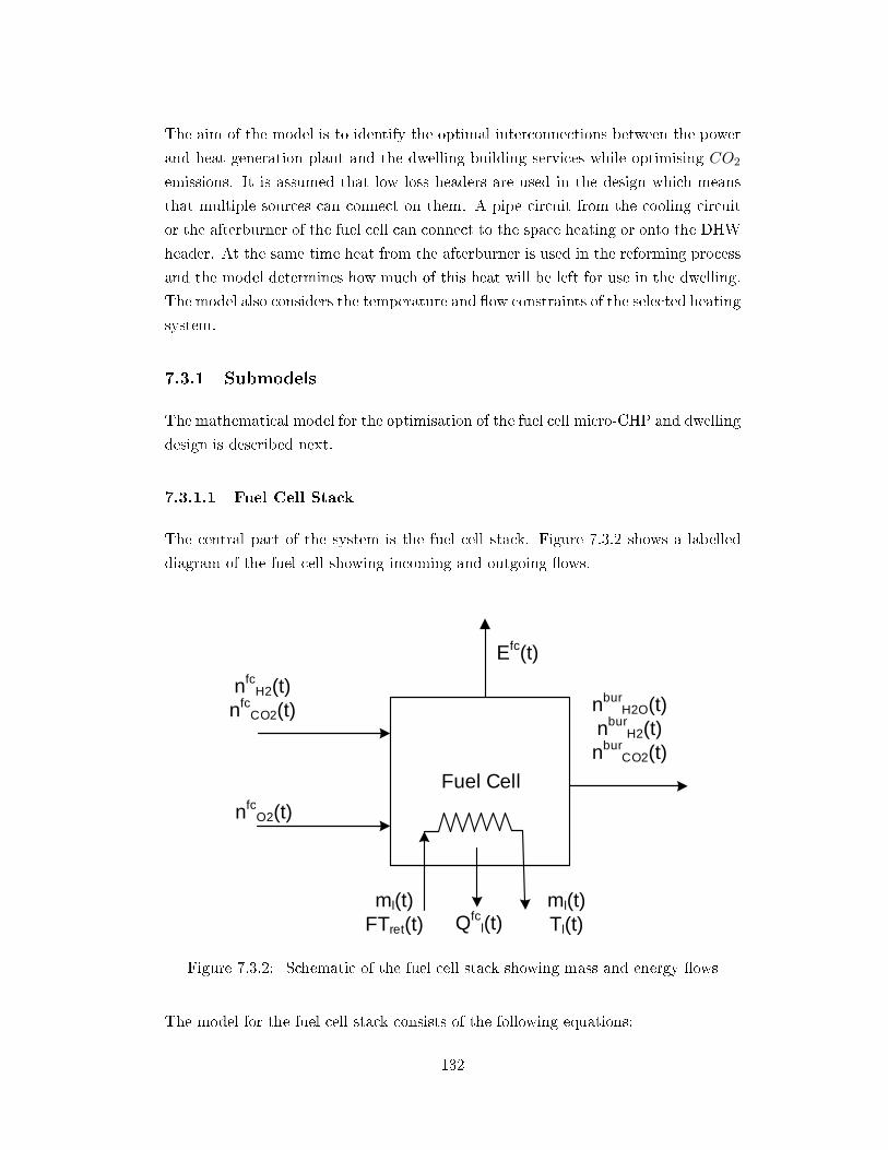
The aim of the model is to identify the optimal interconnections between the power
and heat generation plant and the dwelling building services while optimising CO2
emissions. It is assumed that low loss headers are used in the design which means
that multiple sources can connect on them. A pipe circuit from the cooling circuit
or the afterburner of the fuel cell can connect to the space heating or onto the DHW
header. At the same time heat from the afterburner is used in the reforming process
and the model determines how much of this heat will be left for use in the dwelling.
The model also considers the temperature and �ow constraints of the selected heating
system.
7.3.1 Submodels
The mathematical model for the optimisation of the fuel cell micro-CHP and dwelling
design is described next.
7.3.1.1 Fuel Cell Stack
The central part of the system is the fuel cell stack. Figure 7.3.2 shows a labelled
diagram of the fuel cell showing incoming and outgoing �ows.
Fuel Cell
nfcH2(t)
nfcCO2(t)
Efc(t)
nfcO2(t)
nburH2O(t)
nburH2(t)
nburCO2(t)
Qfcl(t)
ml(t)FTret(t)
ml(t)Tl(t)
Figure 7.3.2: Schematic of the fuel cell stack showing mass and energy �ows
The model for the fuel cell stack consists of the following equations:
132
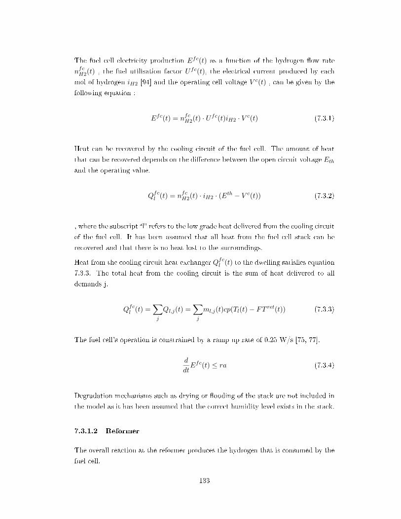
The fuel cell electricity production Efc(t) as a function of the hydrogen �ow rate
nfcH2(t) , the fuel utilisation factor Ufc(t), the electrical current produced by each
mol of hydrogen iH2 [94] and the operating cell voltage V c(t) , can be given by the
following equation :
Efc(t) = nfcH2(t) · Ufc(t)iH2 · V c(t) (7.3.1)
Heat can be recovered by the cooling circuit of the fuel cell. The amount of heat
that can be recovered depends on the di�erence between the open circuit voltage Eth
and the operating value.
Qfcl (t) = nfcH2(t) · iH2 · (Eth − V c(t)) (7.3.2)
, where the subscript �l� refers to the low grade heat delivered from the cooling circuit
of the fuel cell. It has been assumed that all heat from the fuel cell stack can be
recovered and that there is no heat lost to the surroundings.
Heat from the cooling circuit heat exchanger Qfcl (t) to the dwelling satis�es equation
7.3.3. The total heat from the cooling circuit is the sum of heat delivered to all
demands j.
Qfcl (t) =
∑j
Ql,j(t) =∑j
ml,j(t)cp(Tl(t)− FT ret(t)) (7.3.3)
The fuel cell's operation is constrained by a ramp up rate of 0.25 W/s [75, 77].
d
dtEfc(t) ≤ ra (7.3.4)
Degradation mechanisms such as drying or �ooding of the stack are not included in
the model as it has been assumed that the correct humidity level exists in the stack.
7.3.1.2 Reformer
The overall reaction at the reformer produces the hydrogen that is consumed by the
fuel cell.
133
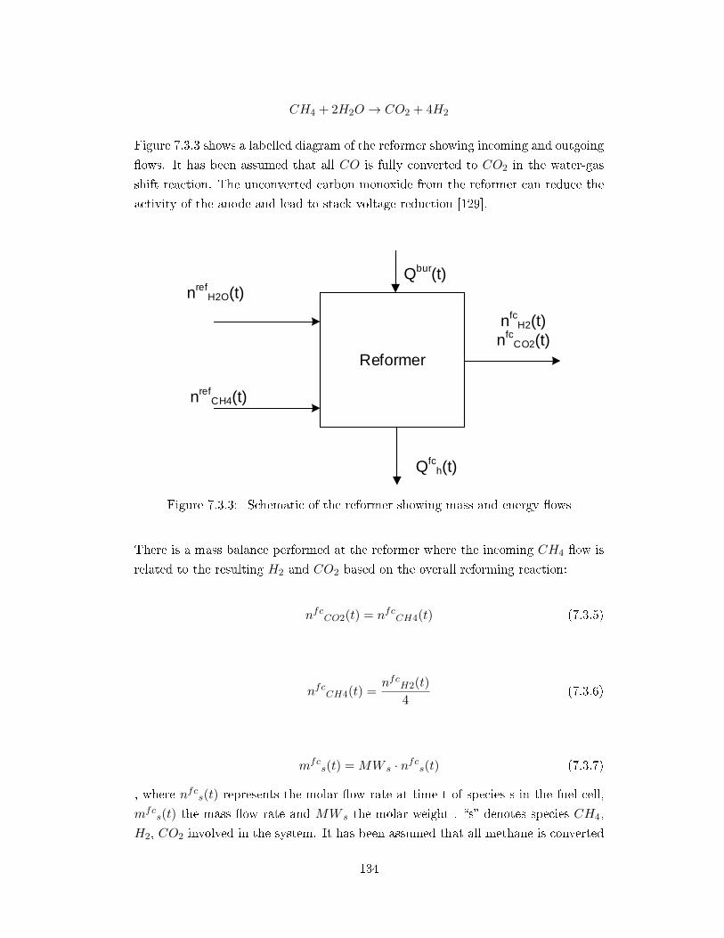
CH4 + 2H2O → CO2 + 4H2
Figure 7.3.3 shows a labelled diagram of the reformer showing incoming and outgoing
�ows. It has been assumed that all CO is fully converted to CO2 in the water-gas
shift reaction. The unconverted carbon monoxide from the reformer can reduce the
activity of the anode and lead to stack voltage reduction [129].
Reformer
nrefCH4(t)
nfcH2(t)
nfcCO2(t)
nrefH2O(t)
Qbur(t)
Qfch(t)
Figure 7.3.3: Schematic of the reformer showing mass and energy �ows
There is a mass balance performed at the reformer where the incoming CH4 �ow is
related to the resulting H2 and CO2 based on the overall reforming reaction:
nfcCO2(t) = nfcCH4(t) (7.3.5)
nfcCH4(t) =nfcH2(t)
4(7.3.6)
mfcs(t) = MW s · nfcs(t) (7.3.7)
, where nfcs(t) represents the molar �ow rate at time t of species s in the fuel cell,
mfcs(t) the mass �ow rate and MW s the molar weight . �s� denotes species CH4,
H2, CO2 involved in the system. It has been assumed that all methane is converted
134
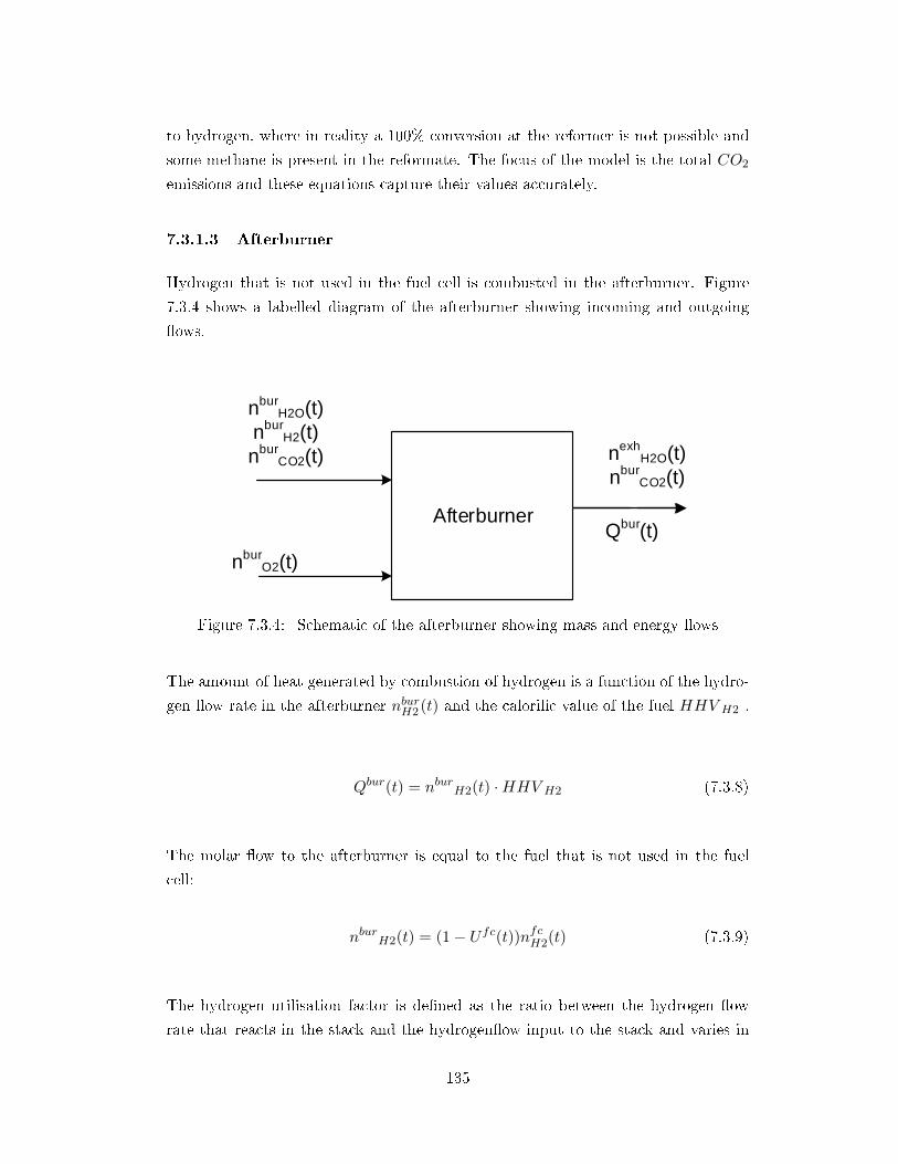
to hydrogen, where in reality a 100% conversion at the reformer is not possible and
some methane is present in the reformate. The focus of the model is the total CO2
emissions and these equations capture their values accurately.
7.3.1.3 Afterburner
Hydrogen that is not used in the fuel cell is combusted in the afterburner. Figure
7.3.4 shows a labelled diagram of the afterburner showing incoming and outgoing
�ows.
Afterburner
nburO2(t)
nexhH2O(t)
nburCO2(t)
Qbur(t)
nburH2O(t)
nburH2(t)
nburCO2(t)
Figure 7.3.4: Schematic of the afterburner showing mass and energy �ows
The amount of heat generated by combustion of hydrogen is a function of the hydro-
gen �ow rate in the afterburner nburH2 (t) and the calori�c value of the fuel HHV H2 .
Qbur(t) = nburH2(t) ·HHV H2 (7.3.8)
The molar �ow to the afterburner is equal to the fuel that is not used in the fuel
cell:
nburH2(t) = (1− Ufc(t))nfcH2(t) (7.3.9)
The hydrogen utilisation factor is de�ned as the ratio between the hydrogen �ow
rate that reacts in the stack and the hydrogen�ow input to the stack and varies in
135
the model between 0.6 to 0.85. Although almost 100% utilisation of hydrogen can
be achieved with dry feeds of hydrogen and oxygen [126], this would require �nding
an alternative source for providing reforming heat such as burning natural gas.
The exhaust gases leave the combustion chamber at 700-800 °C and provide heat
for the reforming process which requires high temperatures to occur [89]. The heat
required for reforming is a function of methane �ow rate nfcCH4(t) and the energy
that is required to reform one mole of CH4 to H2 [89].
Qref (t) = nfcCH4(t) · qref (7.3.10)
Useful heat Qfch (t) can be recovered from the exhaust gases after they have released
heat for the reforming process at 400 °C [89] . The gases enter a heat exchanger
where heat can be recovered and used in the dwelling. It has been assumed that
all heat left in the afterburner exhaust stream after it leaves the reformer can be
recovered.
Qfch (t) = Qbur(t)−Qref (t) (7.3.11)
The remaining heat is recovered by a heat exchanger and it can be used for space
heating, DHW or stored in the TST (all demands are represented by set j). This
heat is modelled using Equation 7.3.12.
Qfch (t) =
∑j
Qh,j(t) =∑j
mh,j(t)cp(Th(t)− FT ret(t)) (7.3.12)
At times when Qbur(t) = Qref (t) there is no remaining heat from the afterburner to
be used in the building as all is used for reforming.
7.3.1.4 Gas Boiler
At the boiler, natural gas is combusted to produce H2O and CO2 based on the
methane combustion reaction. In this case it has been assumed that natural gas is
pure methane
CH4 + 2O2 → CO2 + 2H2O
136
Figure 7.3.5 is a labelled diagram of the gas boiler showing incoming and outgoing
�ows.
Gas Boiler
ngbO2(t)
ngbCH4(t)
ngbCO2(t)
ngbH2O(t)
mgb(t)FTret(t)
mgb(t)Tgb(t)
Figure 7.3.5: Natural Gas Boiler Schematic showing mass and energy �ows
Mass balance is then performed in a similar way at the gas boiler resulting at the
following equations
ngbCO2(t) = ngbCH4(t) (7.3.13)
mgbs(t) = MW sn
gbs(t) (7.3.14)
,where ngbs(t) represents the molar �ow rate at time t of species s in the gas boiler
and mgbs(t) the mass �ow rate.
Boiler heat Qgbj (t) to demand j is given by equation 7.3.15, where T gb(t) is the boiler
supply temperature, cp is the speci�c heat capacity of water.
Qgbj (t) =
∑j
mgbj (t) · cp · (T gb(t)− FT ret(t)) (7.3.15)
Boiler heat is also has to satisfy equation 7.3.16.
∑j
Qgbj (t) = ngbCH4(t) ·HHVCH4 · ηgb (7.3.16)
137
,where ηgb represents the e�ciency of the boiler.
Also,
∑j
Qgbj (t) = rgb(t)P gb (7.3.17)
, where rgb(t) represents the load factor and P gb the maximum capacity of the gas
boiler.
7.3.1.5 Thermal Storage Tank
The model for the TST builds up on the storage model presented in Chapter 6. The
energy content of the storage tank Est (kJ) is given by equation 7.3.18 as in Model
1.
Est(t) = V st · ρ · cp · (T st(t)− T emv(t)) (7.3.18)
Energy balance in the storage tank is given by equation7.3.19 .
d
dtEst(t) =
∑g
Qg,sto(t)−∑j
Qjstout(t) (7.3.19)
As there is no heat �ow from the TST to the TST, for j=sto, Qstostout(t)=0.
The additional elements introduced in the model relate to temperature constraints.
There is a temperature limit below which the storage cannot release heat to the
dwelling. A constraint of 40 °C for UFH and 60 °C for radiators has been introduced
in the model before heat can be used for space heating. The constraint is 60 °C for
DHW. This is to ensure that water �ow from the storage is of su�cient temperature
to be used in the pipe circuits that serve the demands.
This constraint was modelled using binary variable ysj(t) which is linked to both Tstand Qstout as shown in equations 7.3.20 ,7.3.21.
Qjstout(t) ≤ Est(t)
ysj(t)
δt(7.3.20)
138
Tjst(t) ≥ Bst
j ysj(t) (7.3.21)
for T stj (t), Qstout
j (t) ≥0.
Storage heat Qstoutj (t) to demand j is given by equation 7.3.22, where mstout
j (t) is the
TST water �ow rate at time t and demand j
Qstoutj (t) =
∑j
mstoutj (t) · cp · (T st(t)− FT ret(t)) (7.3.22)
A constraint was also added to minimise the impact of the initial and �nal conditions
with regard to the thermal mass stored in the TST. This constraint enforces the TST
temperature at the last timestep to be no more than 20 °C lower than the initial
value at the �rst timestep (7.3.23). This way the TST will not release all saved heat
only because it is the last timestep and the impact on the results will be minimised.
T st(tf ) + 20 ≥ T st(t1) (7.3.23)
, where tf is the last timestep of the dataset and t1 the �rst.
Another way to address the issue of receiving heat from the TST that cannot be
accounted in the objective function (whether this is the cost or the CO2 emissions)
is to force the TST temperature at the �rst hour of the day to be equal to the last
hour of the day for all the days of the dataset. This alternative approach has been
studied and is presented in section 7.5.1.3.
No thermal losses are included in the tank model. This assumption is considered
to have small e�ect on the model results because the datasets are small and the
cumulative amount of thermal losses from the TST would not make a signi�cant
di�erence in the objective function or alter the results in terms of system sizing and
operation. Based on the 0.0075 kWh/lday value for heat losses from hot water tanks
used in IES [85], an average size TST of 200 L would require 1.5 kWh of heat from
the fuel cell per day to maintain the initial TST temperature. The total annual heat
loss from the TST would be then 547.5 kWh which is approximately 2.33% of the
total annual combined heat demand for House A which is 23,430.11 kWh. Therefore
heat for TST thermal losses was decided to be left out from the model.
139
Thermal strati�cation is also not included in the TST model. Strati�cation of water
in a tank creates two separate water temperatures at the bottom and top of the
TST. The bene�t of this is that water at a higher temperature at the top can be
used directly to demand, whereas water at the bottom can return to the heat source.
Strati�cation is bene�cial in solar thermal systems where water at the lower part of
the TST is connected to the solar thermal collectors to extract the maximum possible
heat from the heating �uid. In such systems better thermal strati�cation increases
system performance and e�ciency [57, 84]. Having a strati�ed tank in the model
would require additional equations with regard to temperature distribution inside
the tank so in order to keep the model simple, a non-strati�ed hot water storage
tank is assumed. Celador et al. studied the e�ect of di�erent modelling approaches
of the TST (with or without strati�cation) on the economic feasibility of residential
CHP plants and found di�erences between the results of the feasibility studies. The
pro�ts generated by the system were dependent to the TST modelling approach and
the system with strati�cation had the shortest payback period [33]. However, as the
strati�cation element is missing on all the case studies presented here and since the
approach involves comparison between di�erent scenarios, the main outcomes are
expected not to be a�ected by this omission.
7.3.1.6 Pipe network and Heat Emitters
Water �ows are mixed in the two headers, at the storage tank and at the return,
after all �ow pipework has released their heat to the demand.
Water mass balances are performed in the pipework network where di�erent �ows
come together i.e.
mtotalj (t) = mh,j(t) +ml,j(t) +mgb
j (t) +mstoutj (t) (7.3.24)
,where mtotalj (t) is the total �ow rate to each heat demand, mh,j(t) and ml,j(t)
are the �ow rates from afterburner heat exchanger and the fuel cell cooling circuit
respectively, mgbj is the boiler �ow rate and mstout
j (t) is the �ow rate from the storage
tank.
Variables mstoutj (t) and mgb
j (t) are 0 for j=sto as there is no heat �ow to the TST
from the boiler or TST itself.
The lower bounds for all the individual water �ows are 0, as the results could propose
that heat from the FC cooling circuit is only used for space heating and not for DHW.
140

Therefore these �ows should be able to reach 0 values.
The water mass �ow required for the space heating and DHW in order to maintaina 10 oC temperature di�erence in the demand side is calculated in each step usingthe following relation :
mtotalj (t) =
Qreqj (t)
Cpw · 10for j = HEAT,DHW (7.3.25)
A variable �ow water system has been assumed for the design which varies in each
timestep providing heat to the demand. In such as system an adjustment in output
requires a water �ow change.
Also,
Qreqj (t) = Qgb
j (t) +Qstoutj (t) +
∑g
Qg,j(t) (7.3.26)
The term∑gQg,j(t) represents the summation of the amount of heat delivered to
demand j from the g fuel cell heat exchanger.
Heat emission from the heating and DHW system also needs to satisfy the following
equation:
Qreqj = mtotal
j (t) · cp · (FTsup,j(t)− FTret,j(t)) (7.3.27)
Binary variables have been used in the model in de�nitions of upper and lower
bounds of heat output variables. Binary variables are also used in the mass balances
to force the plant mass �ow rates to become zero when the heat emission is zero. By
using this method temperature constraints between variables are not needed. This
is shown in the following equations:
Qjgb(t) ≤ ygbj (t)Agb
j (7.3.28)
Qjgb(t) ≥ 0.001ygbj (t) (7.3.29)
141
, where Agbj is the upper bound of the heat output of the boiler per demand j
Similarly, binaries ygj(t) , are used for the fuel cell heat exchangers and for the TST
output to each demand.
Qg,j(t) ≤ yfcg,j(t)Afcg,j (7.3.30)
Qg,j(t) ≥ 0.001yfcg,j(t) (7.3.31)
,where Afcg,j is the upper bound of the heat output of heat exchanger g to demand j.
Therefore the mass balance becomes:
mtotalj (t) = ygb(t)mgb
j (t) + ystoutj (t)mstoutj (t) +
∑g
(yg,j(t)mg,j(t)) (7.3.32)
7.3.1.7 Electricity Energy Balance
The electricity output of the fuel cell at time t Efc(t) and the electricity import from
the grid at Eg(t) time t have to be equal to the electricity demand Qreqele (t) as shown
in equation 7.3.33
Qreqele (t) = Efc(t) + Eg(t) (7.3.33)
7.3.1.8 Total System CO2 emissions
The objective function that is minimised here is the total system CO2 emissions
resulting from the operation of the fuel cell and gas boiler and the imported grid
electricity. For the grid electricity, emissions rates for every unit of energy have been
used, as described in [50]. As mentioned earlier, many studies have chosen cost as
their objective function. According to Sta�ell et al. though �There is considerable
uncertainty in the cost targets for fuel cell CHP� [111]. This uncertainty would be
carried on the results of any modelling attempt based on cost. The CO2 emissions on
the other hand, is frees of this problem as it depends on plant e�ciencies and energy
142
balances. Therefore the CO2 emissions as an objective function could represent with
more accuracy than cost, a model that attempts to design a system such as the one
shown in 7.3.1.
Mfc =∑t
mfcCO2(t) (7.3.34)
Mgb =∑t
mgbCO2(t) (7.3.35)
M el = fe∑t
Eg(t) (7.3.36)
min z = Mfc +M el +Mgb (7.3.37)
7.4 Formulation and Solution Approach
The system was modelled in GAMS 23.8. Various MINLP solvers were used on an
Intel Core i5-2500 CPU, 4 GB RAM, 3.3 GHz computer.
The overall problem is formulated as mixed integer non-linear programming (MINLP)
model. Binary variables are used to introduce links between variables. The resulting
optimisation model is non-linear and non-convex.
The analysis is made on a 288-hour dataset of energy demands which is extracted
from the 8760 hour dataset presented in chapter 5. A month, therefore is represented
by 24 hours. This is a more complete dataset than the 48-hour used in the previous
model as it can capture better the variation of space heating demand during the
year. However, because of the use of larger dataset, the size of the problem becomes
big which makes the problem di�cult to solve. Trying to solve the MINLP resulted
in many of the cases in no solution or into very large CPU times, therefore a two-
stage solution was implemented to identify the optimal design and operation of the
fuel cell micro-CHP - dwelling system. At stage 1 a simpler MINLP that does not
take into account the complete pipe network and all system temperatures is solved.
143

Speci�cally equations 7.3.3, 7.3.12, 7.3.15, 7.3.22, 7.3.24, 7.3.25, 7.3.27, 7.3.32 are
not included in the model at stage 1. At the same time candidate starting points for
all variables are introduced to assist the solver to reach a global optimum solution.
At stage 2 the complete MINLP with all equations as described above is solved. The
initial solutions of stage 1 are used as good starting point for solving the complete
model at stage 2. For the stage 1 the solver BARON was used and to be followed
by SBB in stage 2 [67, 104].
All case studies were run using a 1% optimality limit.
The parameters and the bounds of variables are shown in Tables 7.1 and 7.2.
144
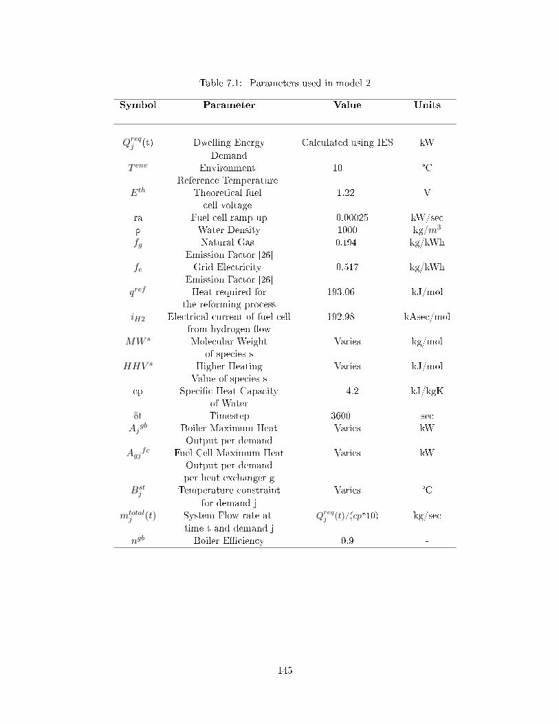
Table 7.1: Parameters used in model 2
Symbol Parameter Value Units
Qreqj (t) Dwelling Energy Calculated using IES kW
DemandT env Environment 10 °C
Reference TemperatureEth Theoretical fuel 1.22 V
cell voltagera Fuel cell ramp up 0.00025 kW/secρ Water Density 1000 kg/m3
fg Natural Gas 0.194 kg/kWhEmission Factor [26]
fe Grid Electricity 0.517 kg/kWhEmission Factor [26]
qref Heat required for 193.06 kJ/molthe reforming process
iH2 Electrical current of fuel cell 192.98 kAsec/molfrom hydrogen �ow
MW s Molecular Weight Varies kg/molof species s
HHV s Higher Heating Varies kJ/molValue of species s
cp Speci�c Heat Capacity 4.2 kJ/kgKof Water
δt Timestep 3600 secAj
gb Boiler Maximum Heat Varies kWOutput per demand
Agjfc Fuel Cell Maximum Heat Varies kW
Output per demandper heat exchanger g
Bstj Temperature constraint Varies °C
for demand jmtotal
j (t) System Flow rate at Qreqj (t)/(cp*10) kg/sec
time t and demand jngb Boiler E�ciency 0.9 -
145
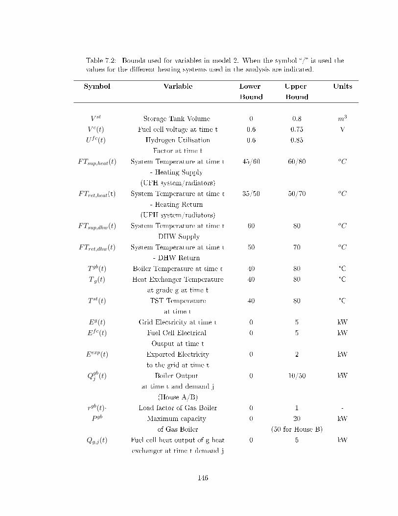
Table 7.2: Bounds used for variables in model 2. When the symbol �/� is used thevalues for the di�erent heating systems used in the analysis are indicated.
Symbol Variable Lower Upper Units
Bound Bound
V st Storage Tank Volume 0 0.8 m3
V c(t) Fuel cell voltage at time t 0.6 0.75 V
Ufc(t) Hydrogen Utilisation 0.6 0.85
Factor at time t
FTsup,heat(t) System Temperature at time t 45/60 60/80 oC
- Heating Supply
(UFH system/radiators)
FTret,heat(t) System Temperature at time t 35/50 50/70 oC
- Heating Return
(UFH system/radiators)
FTsup,dhw(t) System Temperature at time t 60 80 oC
- DHW Supply
FTret,dhw(t) System Temperature at time t 50 70 oC
- DHW Return
T gb(t) Boiler Temperature at time t 40 80 °C
T g(t) Heat Exchanger Temperature 40 80 °C
at grade g at time t
T st(t) TST Temperature 40 80 °C
at time t
Eg(t) Grid Electricity at time t 0 5 kW
Efc(t) Fuel Cell Electrical 0 5 kW
Output at time t
Eexp(t) Exported Electricity 0 2 kW
to the grid at time t
Qgbj (t) Boiler Output 0 10/50 kW
at time t and demand j
(House A/B)
rgb(t)· Load factor of Gas Boiler 0 1 -
P gb Maximum capacity 0 20 kW
of Gas Boiler (50 for House B)
Qg,j(t) Fuel cell heat output of g heat 0 5 kW
exchanger at time t demand j
146
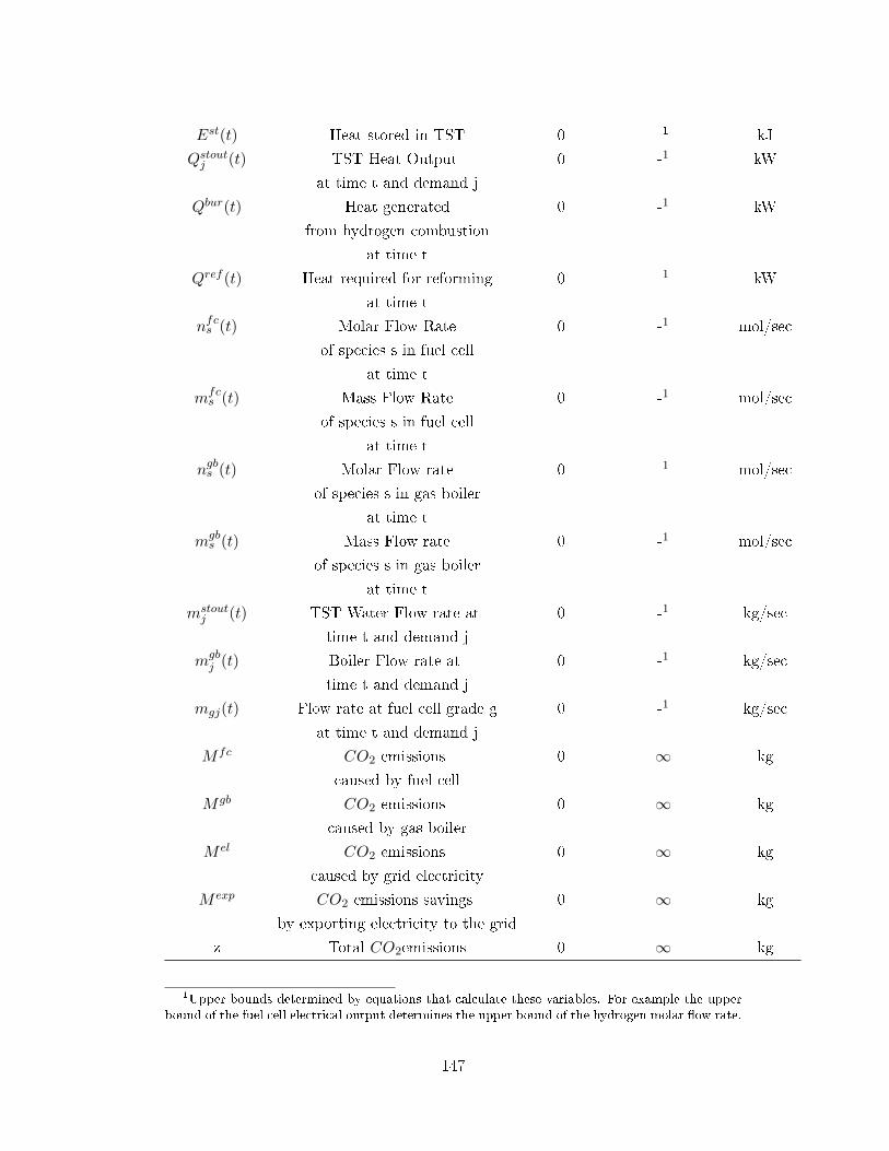
Est(t) Heat stored in TST 0 -1 kJ
Qstoutj (t) TST Heat Output 0 -1 kW
at time t and demand j
Qbur(t) Heat generated 0 -1 kW
from hydrogen combustion
at time t
Qref (t) Heat required for reforming 0 -1 kW
at time t
nfcs (t) Molar Flow Rate 0 -1 mol/sec
of species s in fuel cell
at time t
mfcs (t) Mass Flow Rate 0 -1 mol/sec
of species s in fuel cell
at time t
ngbs (t) Molar Flow rate 0 -1 mol/sec
of species s in gas boiler
at time t
mgbs (t) Mass Flow rate 0 -1 mol/sec
of species s in gas boiler
at time t
mstoutj (t) TST Water Flow rate at 0 -1 kg/sec
time t and demand j
mgbj (t) Boiler Flow rate at 0 -1 kg/sec
time t and demand j
mgj(t) Flow rate at fuel cell grade g 0 -1 kg/sec
at time t and demand j
Mfc CO2 emissions 0 ∞ kg
caused by fuel cell
Mgb CO2 emissions 0 ∞ kg
caused by gas boiler
M el CO2 emissions 0 ∞ kg
caused by grid electricity
M exp CO2 emissions savings 0 ∞ kg
by exporting electricity to the grid
z Total CO2emissions 0 ∞ kg
1Upper bounds determined by equations that calculate these variables. For example the upperbound of the fuel cell electrical output determines the upper bound of the hydrogen molar �ow rate.
147
7.5 Modelling Results
The presentation of the results focuses on highlighting the di�erences in modelling
the various case studies. In addition, the graphs presented in each section are not
repeated throughout if the repetition is not necessary to discuss a point made. An
e�ort has been made to include many case studies and to create a broad view of fuel
cell micro-CHP design and how this can vary in di�erent buildings and scenarios.
The majority of the case studies that are presented here are for House A, the Part
L dwelling. Case study 7 is for the typical UK dwelling.
7.5.1 Part L Dwelling Designed with UFH
Using the model presented above, two fuel cell micro-CHP designs are evaluated in
terms of their CO2 emissions and compared to the base case. The e�ect of TST
in the design and operation of a Part L compliant building is tested by selecting to
evaluate one design option without thermal storage (Case 1) and one with (Case 2).
7.5.1.1 Case 1
The optimum design is illustrated in Figure 7.5.1. All possible connections from
the fuel cell heat exchangers are selected. The cooling circuit and afterburner are
supplying heat to the space heating circuit, the DHW and to the TST. However, the
amounts of heat that each source is supplying to each demand vary. The fuel cell
is sized at 1.9 kWe and the boiler peaks at 5.6 kWth and 1.0 kWth for heating and
DHW respectively. The total CO2 emissions for this case are 211 kgCO2.
148
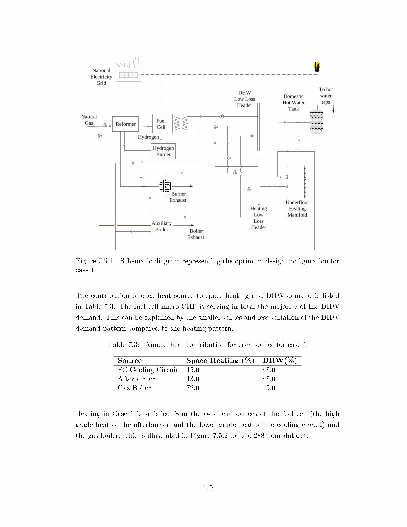
Domestic Hot Water
Tank
Underfloor Heating
Manifold
DHW Low Loss
Header
Heating Low Loss
Header
To hot water taps
Fuel Cell
Burner Exhaust
Auxiliary Boiler
Reformer
Hydrogen Burner
National Electricity
Grid
Natural Gas
Boiler Exhaust
Hydrogen
Figure 7.5.1: Schematic diagram representing the optimum design con�guration forcase 1
The contribution of each heat source to space heating and DHW demand is listed
in Table 7.3. The fuel cell micro-CHP is serving in total the majority of the DHW
demand. This can be explained by the smaller values and less variation of the DHW
demand pattern compared to the heating pattern.
Table 7.3: Annual heat contribution for each source for case 1
Source Space Heating (%) DHW(%)
FC Cooling Circuit 15.0 48.0Afterburner 13.0 43.0Gas Boiler 72.0 9.0
Heating in Case 1 is satis�ed from the two heat sources of the fuel cell (the high
grade heat of the afterburner and the lower grade heat of the cooling circuit) and
the gas boiler. This is illustrated in Figure 7.5.2 for the 288 hour dataset.
149
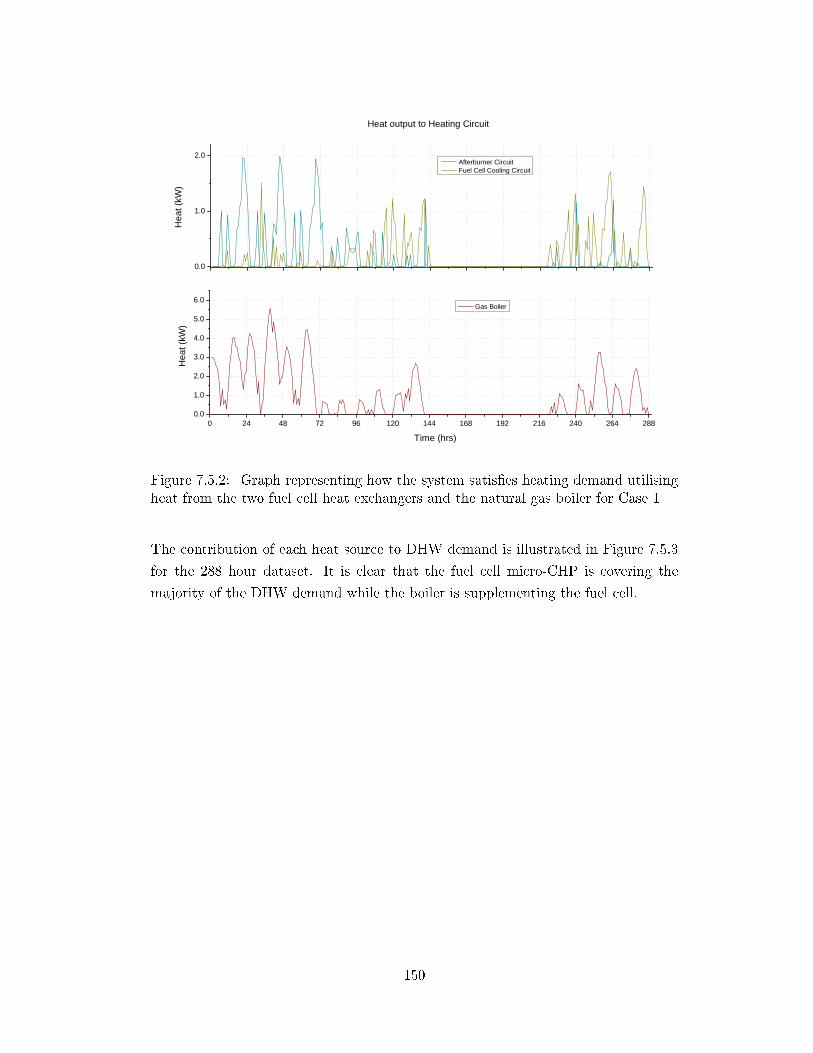
0 . 0
1 . 0
2 . 0
0 2 4 4 8 7 2 9 6 1 2 0 1 4 4 1 6 8 1 9 2 2 1 6 2 4 0 2 6 4 2 8 80 . 01 . 02 . 03 . 04 . 05 . 06 . 0
A f t e r b u r n e r C i r c u i t F u e l C e l l C o o l i n g C i r c u i t
Heat
(kW)
Heat
(kW)
T i m e ( h r s )
G a s B o i l e r
H e a t o u t p u t t o H e a t i n g C i r c u i t
Figure 7.5.2: Graph representing how the system satis�es heating demand utilisingheat from the two fuel cell heat exchangers and the natural gas boiler for Case 1
The contribution of each heat source to DHW demand is illustrated in Figure 7.5.3
for the 288 hour dataset. It is clear that the fuel cell micro-CHP is covering the
majority of the DHW demand while the boiler is supplementing the fuel cell.
150
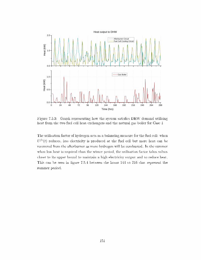
0 . 0
1 . 0
2 . 0
0 2 4 4 8 7 2 9 6 1 2 0 1 4 4 1 6 8 1 9 2 2 1 6 2 4 0 2 6 4 2 8 80 . 0
0 . 5
1 . 0
A f t e r b u r n e r C i r c u i t F u e l C e l l C o o l i n g C i r c u i t
Heat
(kW)
Heat
(kW)
T i m e ( h r s )
G a s B o i l e r
H e a t o u t p u t t o D H W
Figure 7.5.3: Graph representing how the system satis�es DHW demand utilisingheat from the two fuel cell heat exchangers and the natural gas boiler for Case 1
The utilisation factor of hydrogen acts as a balancing measure for the fuel cell: when
Ufc(t) reduces, less electricity is produced at the fuel cell but more heat can be
recovered from the afterburner as more hydrogen will be combusted. In the summer
when less heat is required than the winter period, the utilisation factor takes values
closer to its upper bound to maintain a high electricity output and to reduce heat.
This can be seen in �gure 7.5.4 between the hours 144 to 216 that represent the
summer period.
151
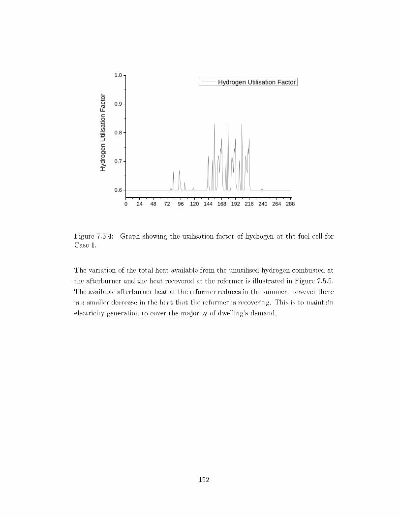
0 2 4 4 8 7 2 9 6 1 2 0 1 4 4 1 6 8 1 9 2 2 1 6 2 4 0 2 6 4 2 8 8
0 . 6
0 . 7
0 . 8
0 . 9
1 . 0
Hydro
gen U
tilisati
on Fa
ctor
H y d r o g e n U t i l i s a t i o n F a c t o r
Figure 7.5.4: Graph showing the utilisation factor of hydrogen at the fuel cell forCase 1.
The variation of the total heat available from the unutilised hydrogen combusted at
the afterburner and the heat recovered at the reformer is illustrated in Figure 7.5.5.
The available afterburner heat at the reformer reduces in the summer, however there
is a smaller decrease in the heat that the reformer is recovering. This is to maintain
electricity generation to cover the majority of dwelling's demand.
152
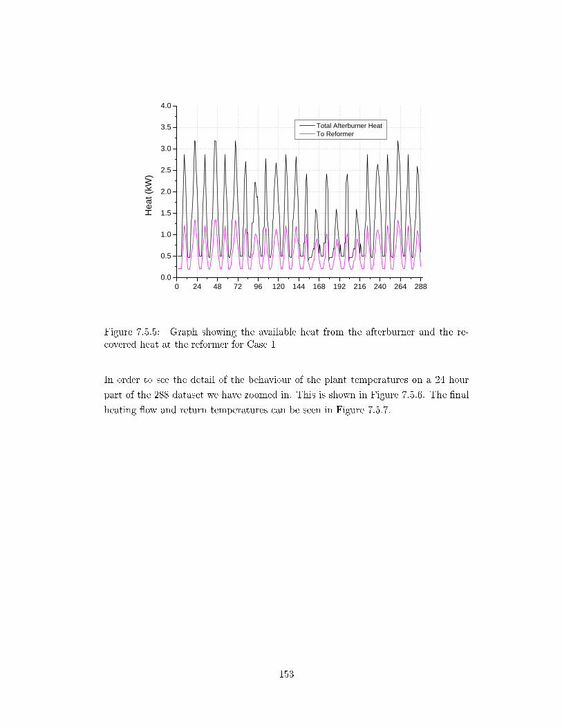
0 2 4 4 8 7 2 9 6 1 2 0 1 4 4 1 6 8 1 9 2 2 1 6 2 4 0 2 6 4 2 8 80 . 0
0 . 5
1 . 0
1 . 5
2 . 0
2 . 5
3 . 0
3 . 5
4 . 0
Heat
(kW)
T o t a l A f t e r b u r n e r H e a t T o R e f o r m e r
Figure 7.5.5: Graph showing the available heat from the afterburner and the re-covered heat at the reformer for Case 1
In order to see the detail of the behaviour of the plant temperatures on a 24 hour
part of the 288 dataset we have zoomed in. This is shown in Figure 7.5.6. The �nal
heating �ow and return temperatures can be seen in Figure 7.5.7.
153
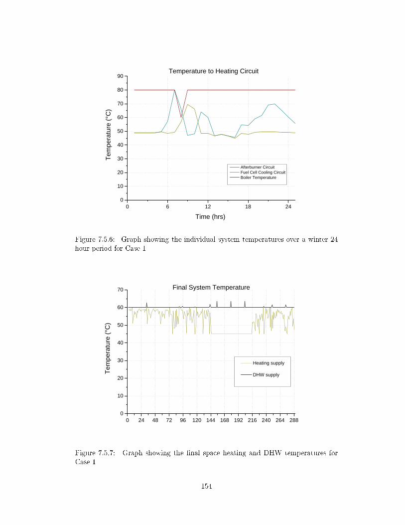
0 6 1 2 1 8 2 40
1 0
2 0
3 0
4 0
5 0
6 0
7 0
8 0
9 0 T e m p e r a t u r e t o H e a t i n g C i r c u i t
T i m e ( h r s )
Temp
eratur
e (°C
)
A f t e r b u r n e r C i r c u i t F u e l C e l l C o o l i n g C i r c u i t B o i l e r T e m p e r a t u r e
Figure 7.5.6: Graph showing the individual system temperatures over a winter 24hour period for Case 1
0 2 4 4 8 7 2 9 6 1 2 0 1 4 4 1 6 8 1 9 2 2 1 6 2 4 0 2 6 4 2 8 80
1 0
2 0
3 0
4 0
5 0
6 0
7 0
H e a t i n g s u p p l y D H W s u p p l yTe
mpera
ture (
°C)
F i n a l S y s t e m T e m p e r a t u r e
Figure 7.5.7: Graph showing the �nal space heating and DHW temperatures forCase 1
154

The �nal temperatures maintain a 10 oC di�erence throughout. In the summer,
between hours 144 and 216 space heating demand is 0, so the heating supply variable
takes the value of the lower bound. At the same time the �ow rate to heating is
0 as it can be seen from the �gure 7.5.8. The �ow rate data obtained from the
results help designers and manufacturers determine the maximum �ows of heating
and DHW circulation pumps.
0 2 4 4 8 7 2 9 6 1 2 0 1 4 4 1 6 8 1 9 2 2 1 6 2 4 0 2 6 4 2 8 80 . 0 0
0 . 0 4
0 . 0 8
0 . 1 2
0 . 1 6
0 . 2 0
Water
Flow
Rate
(kg/se
c)
H e a t i n g F l o w r a t e
Figure 7.5.8: Graph showing the total water �ow from the heating header to theUFH manifold for Case 1. The water �ow is 0 in the summer months when spaceheating demand is 0.
The electricity generation from the fuel cell and the electricity grid input is depicted
in Figure 7.5.9. At the last few hours of the dataset the fuel cell electricity drops and
import from the grid increases. This is because the fuel cell is gradually ramping
down to eventually stop as it approaches the �nal steps of the dataset. This is an
issue raised in the discussion of the previous model with regard to the thermal mass
of the TST and can also be seen here. It is an edge e�ect in the sense that the
end of the dataset a�ects the values of the variables. This can be observed in both
models and happens because the models consider only the data given and not what
happens after the last timestep. However, in reality there is a continuity in any
dataset whether this is 288 or 8760 hours. The impact on the results increases as
the dataset becomes smaller.
155
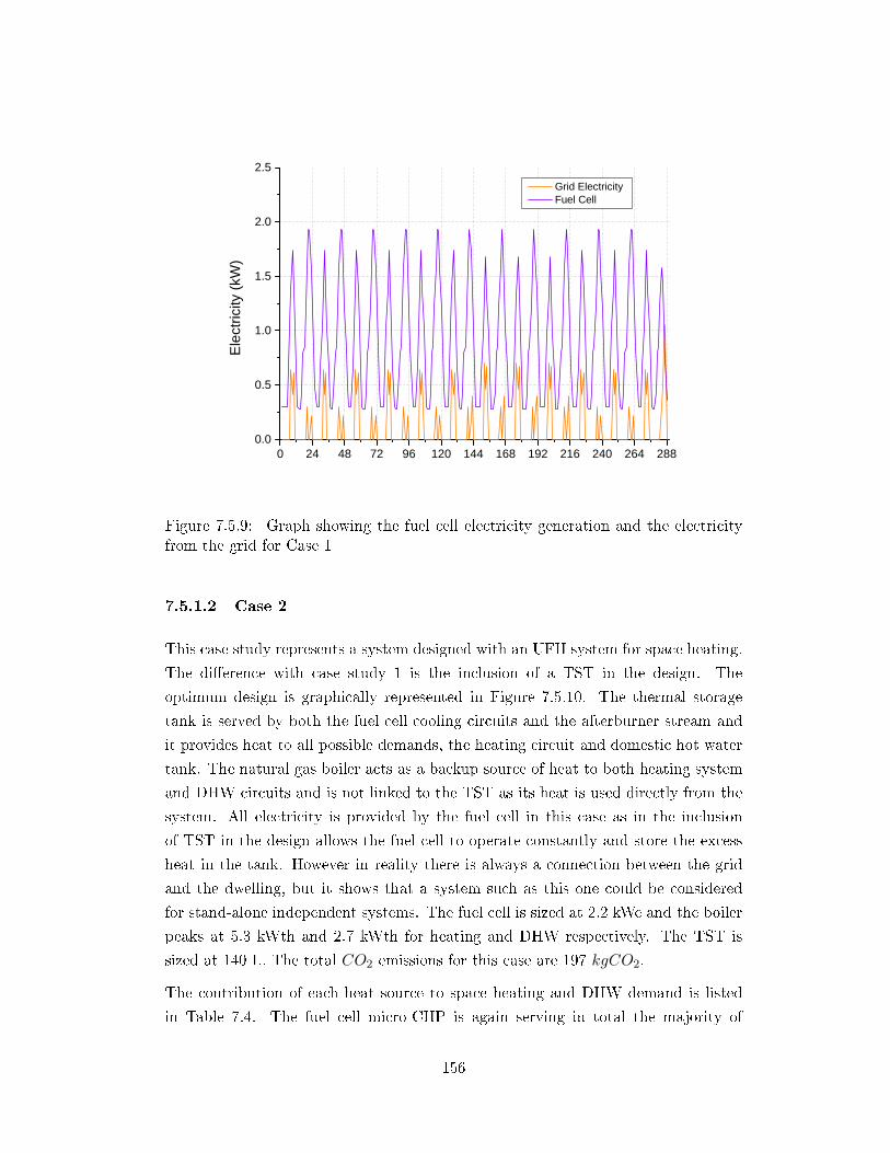
0 2 4 4 8 7 2 9 6 1 2 0 1 4 4 1 6 8 1 9 2 2 1 6 2 4 0 2 6 4 2 8 80 . 0
0 . 5
1 . 0
1 . 5
2 . 0
2 . 5 G r i d E l e c t r i c i t y F u e l C e l l
Electr
icity (
kW)
Figure 7.5.9: Graph showing the fuel cell electricity generation and the electricityfrom the grid for Case 1
7.5.1.2 Case 2
This case study represents a system designed with an UFH system for space heating.
The di�erence with case study 1 is the inclusion of a TST in the design. The
optimum design is graphically represented in Figure 7.5.10. The thermal storage
tank is served by both the fuel cell cooling circuits and the afterburner stream and
it provides heat to all possible demands, the heating circuit and domestic hot water
tank. The natural gas boiler acts as a backup source of heat to both heating system
and DHW circuits and is not linked to the TST as its heat is used directly from the
system. All electricity is provided by the fuel cell in this case as in the inclusion
of TST in the design allows the fuel cell to operate constantly and store the excess
heat in the tank. However in reality there is always a connection between the grid
and the dwelling, but it shows that a system such as this one could be considered
for stand-alone independent systems. The fuel cell is sized at 2.2 kWe and the boiler
peaks at 5.3 kWth and 2.7 kWth for heating and DHW respectively. The TST is
sized at 140 L. The total CO2 emissions for this case are 197 kgCO2.
The contribution of each heat source to space heating and DHW demand is listed
in Table 7.4. The fuel cell micro-CHP is again serving in total the majority of
156

the DHW demand which has lower values and less variation compared to the space
heating demand. The total heat output of the fuel cell micro-CHP system have been
increased approximately 7% compared to case 1.
Domestic Hot Water Tank
Underfloor Heating
Manifold
DHW Low Loss
Header
Heating Low Loss
Header
To hot water taps
Fuel Cell
Afterburner Exhaust
Auxiliary Boiler
Thermal Storage Tank
High Grade
Heat HX
Low Grade Heat HX
Tsu,lowReformer
Afterburner
Natural Gas
Electricity Demand
National Electricity
Grid
Natural Gas
Hydrogen
Electricity
LTHW
Tst
Figure 7.5.10: Schematic diagram representing the optimum design con�gurationfor case 2 showing the TST in addition to the other units and its connections to thesystem
Table 7.4: Annual heat contribution for each source for case 2
Source Space Heating (%) DHW(%)
FC Cooling Circuit 17 36Afterburner 13 30Gas Boiler 60 24TST 4 10
Figure 7.5.11 shows the electricity generation of the fuel cell system. In this case the
operation of the fuel cell is following the electricity demand and there is no import
from the grid.
157
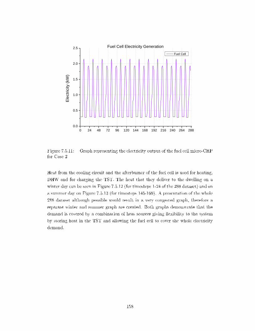
0 2 4 4 8 7 2 9 6 1 2 0 1 4 4 1 6 8 1 9 2 2 1 6 2 4 0 2 6 4 2 8 80 . 0
0 . 5
1 . 0
1 . 5
2 . 0
2 . 5 F u e l C e l l
Electr
icity (
kW)
F u e l C e l l E l e c t r i c i t y G e n e r a t i o n
Figure 7.5.11: Graph representing the electricity output of the fuel cell micro-CHPfor Case 2
Heat from the cooling circuit and the afterburner of the fuel cell is used for heating,
DHW and for charging the TST. The heat that they deliver to the dwelling on a
winter day can be seen in Figure 7.5.12 (for timesteps 1-24 of the 288 dataset) and on
a summer day on Figure 7.5.13 (for timesteps 145-169). A presentation of the whole
288 dataset although possible would result in a very congested graph, therefore a
separate winter and summer graph are created. Both graphs demonstrate that the
demand is covered by a combination of heat sources giving �exibility to the system
by storing heat in the TST and allowing the fuel cell to cover the whole electricity
demand.
158
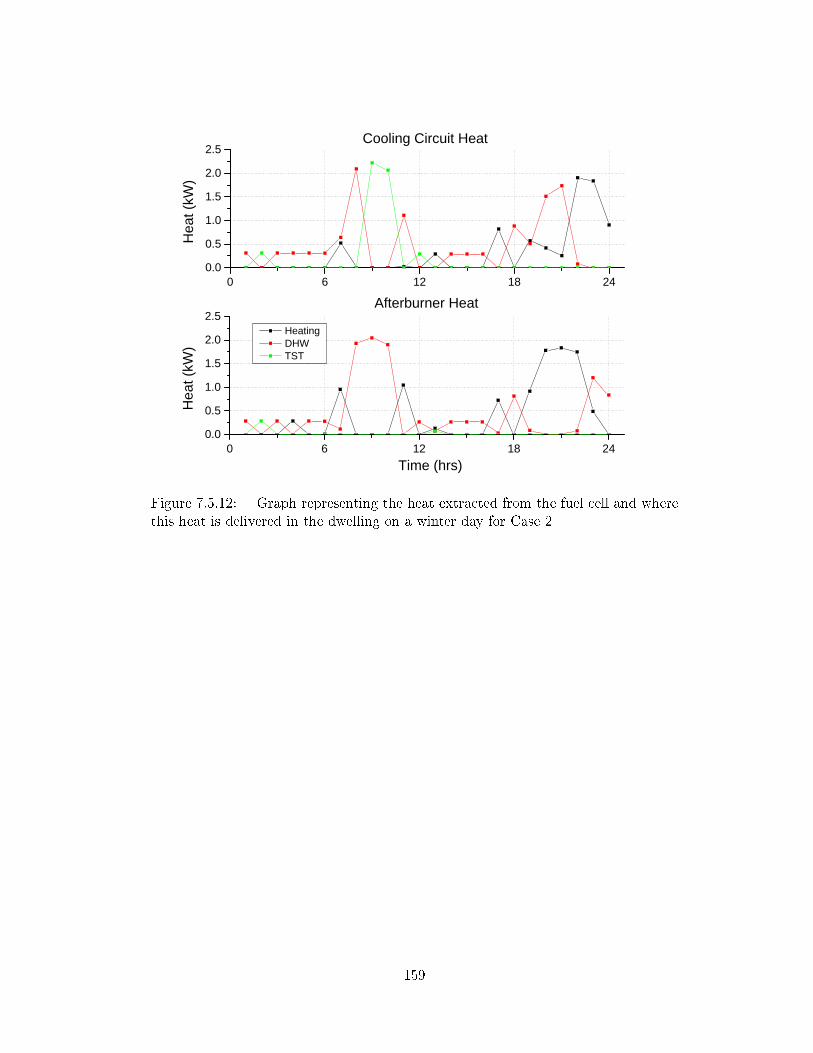
0 6 1 2 1 8 2 40 . 00 . 51 . 01 . 52 . 02 . 5
0 6 1 2 1 8 2 40 . 00 . 51 . 01 . 52 . 02 . 5
Heat
(kW)
C o o l i n g C i r c u i t H e a t
Heat
(kW)
T i m e ( h r s )
H e a t i n g D H W T S T
A f t e r b u r n e r H e a t
Figure 7.5.12: Graph representing the heat extracted from the fuel cell and wherethis heat is delivered in the dwelling on a winter day for Case 2
159
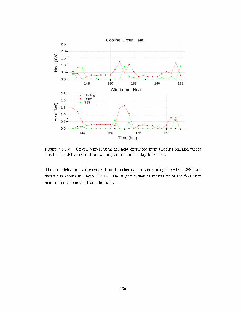
1 4 5 1 5 0 1 5 5 1 6 0 1 6 50 . 00 . 51 . 01 . 52 . 02 . 5
1 4 4 1 5 0 1 5 6 1 6 20 . 00 . 51 . 01 . 52 . 02 . 5
Heat
(kW)
C o o l i n g C i r c u i t H e a t
Heat
(kW)
T i m e ( h r s )
H e a t i n g D H W T S T
A f t e r b u r n e r H e a t
Figure 7.5.13: Graph representing the heat extracted from the fuel cell and wherethis heat is delivered in the dwelling on a summer day for Case 2
The heat delivered and received from the thermal storage during the whole 288 hour
dataset is shown in Figure 7.5.14. The negative sign is indicative of the fact that
heat is being removed from the tank.
160
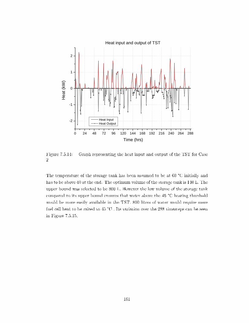
0 2 4 4 8 7 2 9 6 1 2 0 1 4 4 1 6 8 1 9 2 2 1 6 2 4 0 2 6 4 2 8 8
- 2
- 1
0
1
2
H e a t I n p u t H e a t O u t p u t
T i m e ( h r s )
Heat
(kW)
H e a t i n p u t a n d o u t p u t o f T S T
Figure 7.5.14: Graph representing the heat input and output of the TST for Case2
The temperature of the storage tank has been assumed to be at 60 °C initially and
has to be above 40 at the end. The optimum volume of the storage tank is 140 L. The
upper bound was selected to be 800 L. However the low volume of the storage tank
compared to its upper bound ensures that water above the 45 °C heating threshold
would be more easily available in the TST. 800 litres of water would require more
fuel cell heat to be raised to 45 °C . Its variation over the 288 timesteps can be seen
in Figure 7.5.15.
161

0 2 4 4 8 7 2 9 6 1 2 0 1 4 4 1 6 8 1 9 2 2 1 6 2 4 0 2 6 4 2 8 80
1 0
2 0
3 0
4 0
5 0
6 0
7 0
8 0
Temp
eratur
e (°C
)
T i m e ( h r s )
T S T T e m p e r a t u r e
T S T T e m p e r a t u r e
Figure 7.5.15: Graph representing the variation of water temperature in the TSTfor Case 2
0 6 1 2 1 8 2 40
1 0
2 0
3 0
4 0
5 0
6 0
7 0
8 0
T i m e ( h r s )
Temp
eratur
e (°C
)
A f t e r b u r n e r C i r c u i t F u e l C e l l C o o l i n g C i r c u i t
T e m p e r a t u r e t o H e a t i n g C i r c u i t
Figure 7.5.16: Graph showing the individual system temperatures over a winter 24hour period for Case 2
162
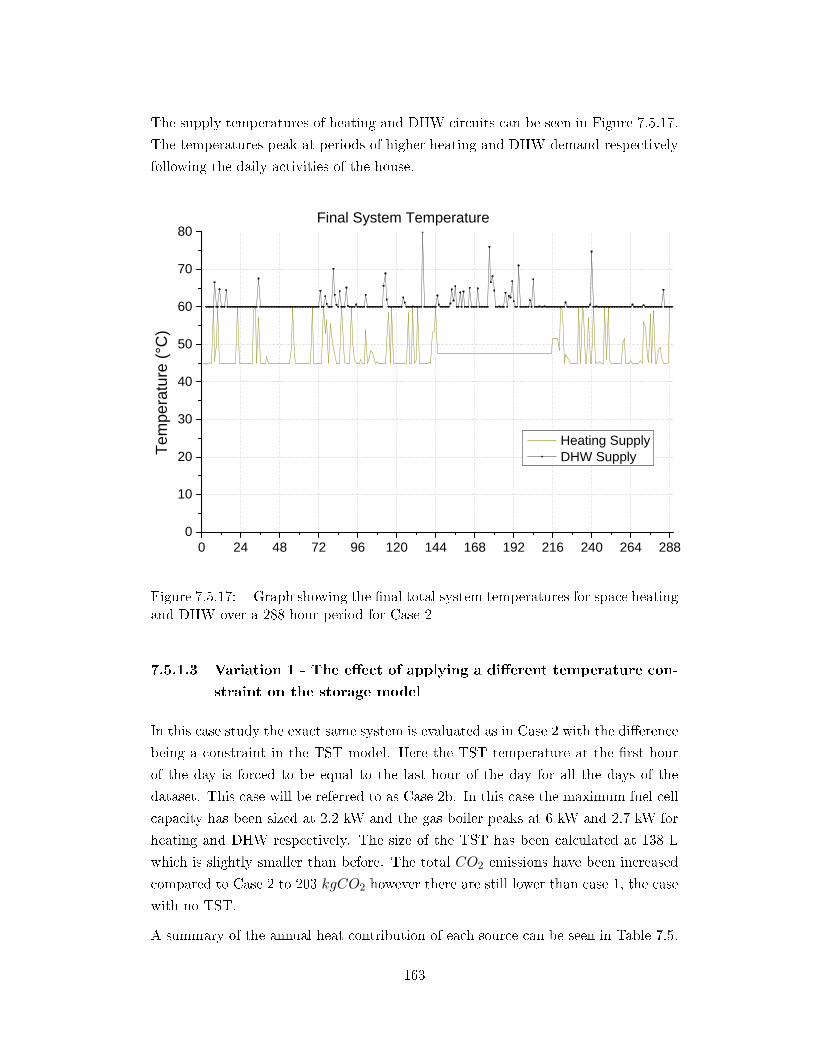
The supply temperatures of heating and DHW circuits can be seen in Figure 7.5.17.
The temperatures peak at periods of higher heating and DHW demand respectively
following the daily activities of the house.
0 2 4 4 8 7 2 9 6 1 2 0 1 4 4 1 6 8 1 9 2 2 1 6 2 4 0 2 6 4 2 8 80
1 0
2 0
3 0
4 0
5 0
6 0
7 0
8 0
H e a t i n g S u p p l y D H W S u p p l yTe
mpera
ture (
°C)
F i n a l S y s t e m T e m p e r a t u r e
Figure 7.5.17: Graph showing the �nal total system temperatures for space heatingand DHW over a 288 hour period for Case 2
7.5.1.3 Variation 1 - The e�ect of applying a di�erent temperature con-
straint on the storage model
In this case study the exact same system is evaluated as in Case 2 with the di�erence
being a constraint in the TST model. Here the TST temperature at the �rst hour
of the day is forced to be equal to the last hour of the day for all the days of the
dataset. This case will be referred to as Case 2b. In this case the maximum fuel cell
capacity has been sized at 2.2 kW and the gas boiler peaks at 6 kW and 2.7 kW for
heating and DHW respectively. The size of the TST has been calculated at 138 L
which is slightly smaller than before. The total CO2 emissions have been increased
compared to Case 2 to 203 kgCO2 however there are still lower than case 1, the case
with no TST.
A summary of the annual heat contribution of each source can be seen in Table 7.5.
163
The total heat from the TST to the heating and DHW has been decreased compared
to Case 2 to only 4% in heating and 3% in DHW. Naturally, the gas boiler's total
heat contribution to both heating and DHW has been increased compared to Case
2.
Table 7.5: Annual heat contribution for each source for Case 2b
Source Space Heating (%) DHW(%)
FC Cooling Circuit 10 34Afterburner 4 9Gas Boiler 82 54TST 4 3
This case study compared to case 2 relies more on the gas boiler for heat production
while the fuel cell operates at a higher average utilisation factor and voltage to favour
electricity production. However because the fuel cell overall is used less than before
there is some grid electricity imported to satisfy demand.
Figure 7.5.18 shows the variation of the TST temperature. It can be seen that at the
end of each day the temperature is equal to the start of the day. In the �gure it is also
shown that the otherwise wasted summer heat is stored in the TST increasing water
temperature. The temperature in the TST increases above 50 °C in the summer
when heat from the fuel cell that is not needed in the system is stored in the TST.
164

0 2 4 4 8 7 2 9 6 1 2 0 1 4 4 1 6 8 1 9 2 2 1 6 2 4 0 2 6 4 2 8 80
1 0
2 0
3 0
4 0
5 0
6 0
7 0
8 0 T S T T e m p e r a t u r e
Temp
eratur
e (°C
)
T i m e ( h r s )
T S T T e m p e r a t u r e
Figure 7.5.18: Graph representing the variation of water temperature in the TSTfor Case 2b
7.5.1.4 Comparative Results
Table 7.6 summarises the basic characteristics of the three designs and of the vari-
ation. The reductions in CO2 emissions from the base case varybetween 27% and
32% respectively. The variation of case 2, case 2b which includes a di�erent approach
in modelling the TST, results in a very similar system to case 2 but with di�erent
operation pattern. The base case emissions are derived from the reference building
presented in chapter 5.
Table 7.6: Summary of results for cases l and 2
CO2 emissions Reduction Boiler CO2 Fuel Cell Grid Electricity
(kgCO2)(%) emissions CO2 emissions CO2 emissions
(kgCO2) (kgCO2) (kgCO2)
Base Case 289 - 161 - 128
Case 1 211 27.0 60 135 16
Case 2 197 31.8 54 143 0
Case 2b 203 29.9 103 98 1
Comparing the cases presented here, the main points are the following:
165
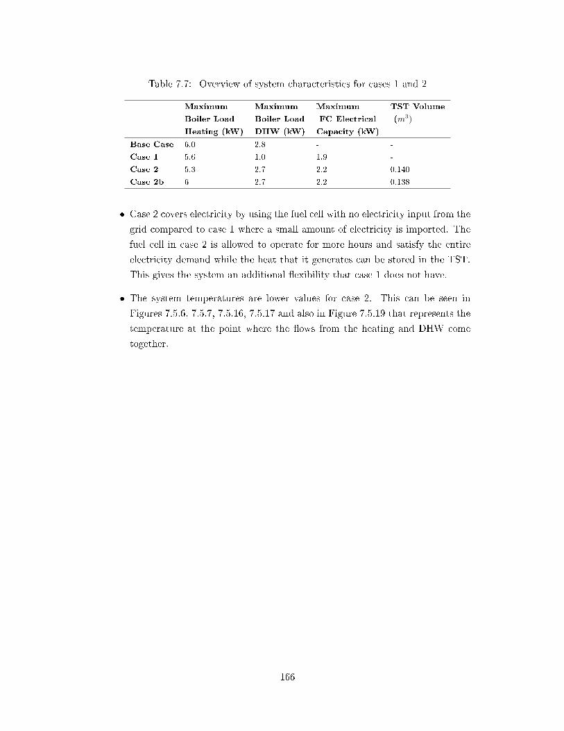
Table 7.7: Overview of system characteristics for cases 1 and 2
Maximum Maximum Maximum TST Volume
Boiler Load Boiler Load FC Electrical (m3)
Heating (kW) DHW (kW) Capacity (kW)
Base Case 6.0 2.8 - -
Case 1 5.6 1.0 1.9 -
Case 2 5.3 2.7 2.2 0.140
Case 2b 6 2.7 2.2 0.138
� Case 2 covers electricity by using the fuel cell with no electricity input from the
grid compared to case 1 where a small amount of electricity is imported. The
fuel cell in case 2 is allowed to operate for more hours and satisfy the entire
electricity demand while the heat that it generates can be stored in the TST.
This gives the system an additional �exibility that case 1 does not have.
� The system temperatures are lower values for case 2. This can be seen in
Figures 7.5.6, 7.5.7, 7.5.16, 7.5.17 and also in Figure 7.5.19 that represents the
temperature at the point where the �ows from the heating and DHW come
together.
166

0 6 1 2 1 8 2 40
1 0
2 0
3 0
4 0
5 0Te
mpera
ture (
°C)
C a s e 2 C a s e 1
R e t u r n T e m p e r a t u r e
Figure 7.5.19: Graph showing the total return system temperatures over a winter24 hour period for Cases 1 and 2
The total boiler CO2 emissions are reduced in Case 2 which together with the higher
sizing of the fuel cell indicates that case 2 relies more on the fuel cell to cover energy
demand. Figure 7.5.20 shows the variation of the total boiler load for the whole 288
period. It can be seen that the boiler in Case 1 is operating in the summer hours
(144 to 216), whereas the boiler in case 2 has turned o�.
167
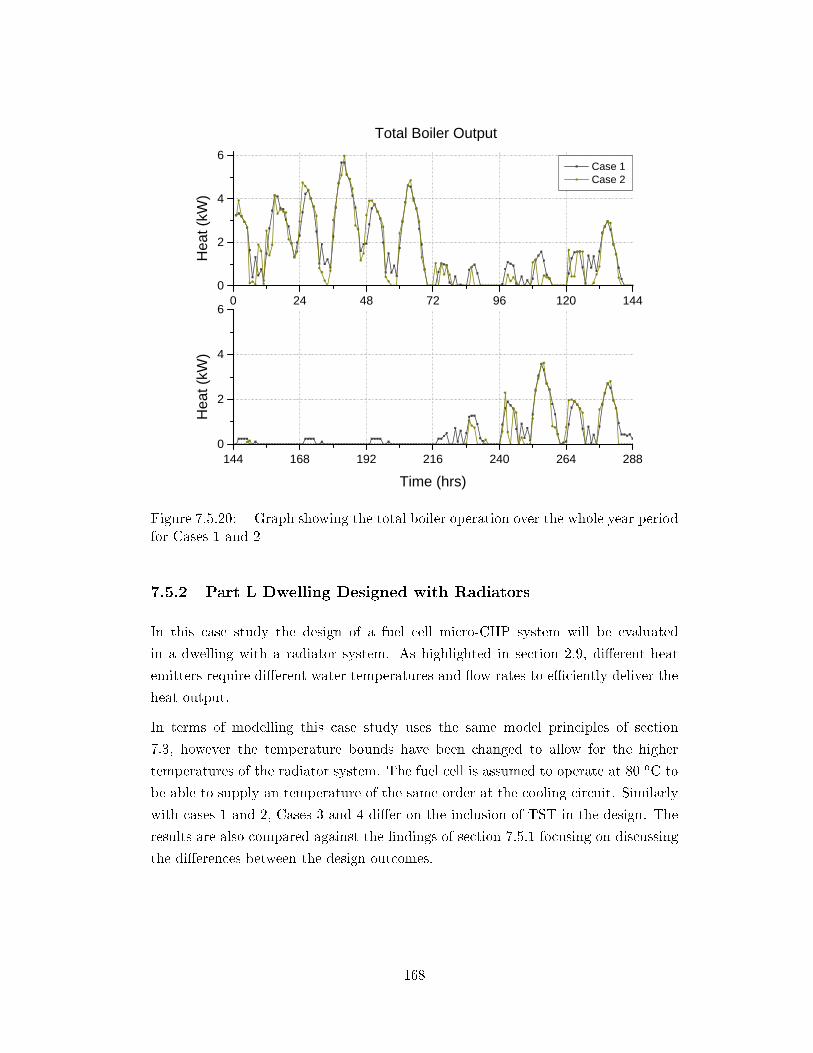
0 2 4 4 8 7 2 9 6 1 2 0 1 4 40
2
4
6 C a s e 1 C a s e 2
Heat
(kW)
T o t a l B o i l e r O u t p u t
1 4 4 1 6 8 1 9 2 2 1 6 2 4 0 2 6 4 2 8 80
2
4
6
Heat
(kW)
T i m e ( h r s )Figure 7.5.20: Graph showing the total boiler operation over the whole year periodfor Cases 1 and 2
7.5.2 Part L Dwelling Designed with Radiators
In this case study the design of a fuel cell micro-CHP system will be evaluated
in a dwelling with a radiator system. As highlighted in section 2.9, di�erent heat
emitters require di�erent water temperatures and �ow rates to e�ciently deliver the
heat output.
In terms of modelling this case study uses the same model principles of section
7.3, however the temperature bounds have been changed to allow for the higher
temperatures of the radiator system. The fuel cell is assumed to operate at 80 oC to
be able to supply an temperature of the same order at the cooling circuit. Similarly
with cases 1 and 2, Cases 3 and 4 di�er on the inclusion of TST in the design. The
results are also compared against the �ndings of section 7.5.1 focusing on discussing
the di�erences between the design outcomes.
168

7.5.2.1 Case 3
The optimum design and the connections from each heat exchanger to heating and
hot water demands are illustrated in Figure 7.5.21. The fuel cell is sized at 2.5kWe
and the boiler at 6.2 kWth and 1.5 kWth for heating and DHW respectively. All
possible heat sources are contributing to satisfying space heating and DHW demand.
169
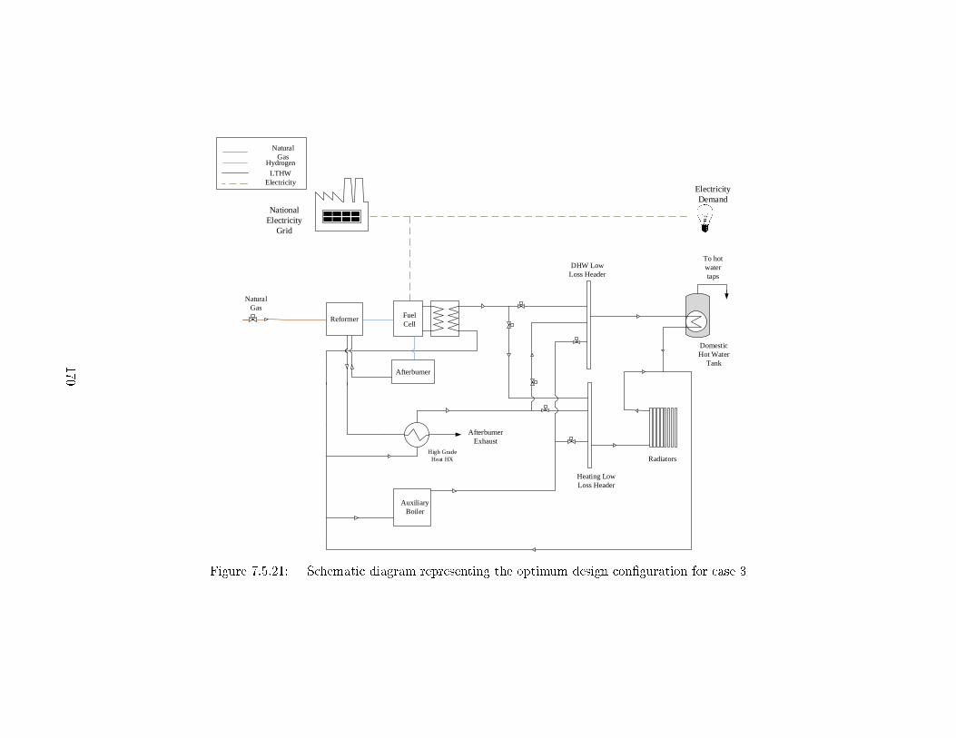
Domestic Hot Water
Tank
DHW Low Loss Header
Heating Low Loss Header
To hot water taps
Fuel Cell
Afterburner Exhaust
Auxiliary Boiler
High Grade Heat HX
Reformer
Afterburner
Natural Gas
Electricity Demand
National Electricity
Grid
Natural Gas
Hydrogen
ElectricityLTHW
Radiators
Figure 7.5.21: Schematic diagram representing the optimum design con�guration for case 3
170
The contribution of each heat source to space heating and DHW demand is listed in
Table 7.8. The fuel cell micro-CHP is serving in total 80% of the DHW demand.
Table 7.8: Annual heat contribution for each source for case 3
Source Space Heating (%) DHW(%)
FC Cooling Circuit 13.0 50.0Afterburner 9.0 30.0Gas Boiler 78.0 20.0
The higher pipe temperatures of the heating system are the characteristic of this
case study. This is best illustrated in Figure 7.5.22 which zooms in again on the 288
dataset to show the pipe temperature leaving the fuel cell cooling circuit and the
afterburner heat exchanger for the �rst 48 hours of the 288 data set. Figure 7.5.23
shows the resulting �nal supply and return pipe temperature at the heating and
DHW circuits. The �nal temperatures in both circuits follow a 10 °C temperature
di�erence while the �ow rate varies to satisfy the demand.
171

6 1 2 1 8 2 4 3 0 3 6 4 2 4 80
1 02 03 04 05 06 07 08 0
Temp
eratur
e (°C
)F C C o o l i n g C i r c u i t t o H e a t i n g
Temp
eratur
e (°C
)
T i m e ( h r s )
6 1 2 1 8 2 4 3 0 3 6 4 2 4 80
1 02 03 04 05 06 07 08 0
A f t e r b u r n e r C i r c u i t t o H e a t i n g
T i m e ( h r s )
0
1
2
3
4
5
Heat
(kW)
0
1
2
3
4
5
Heat
(kW)
Figure 7.5.22: Graph showing the supply temperatures of the fuel cell cooling circuitand afterburner heat exchangers over a period of 48 hours for Case 3. Additionallythe heat output of each heat exchanger to space heating is shown on the right axis
172
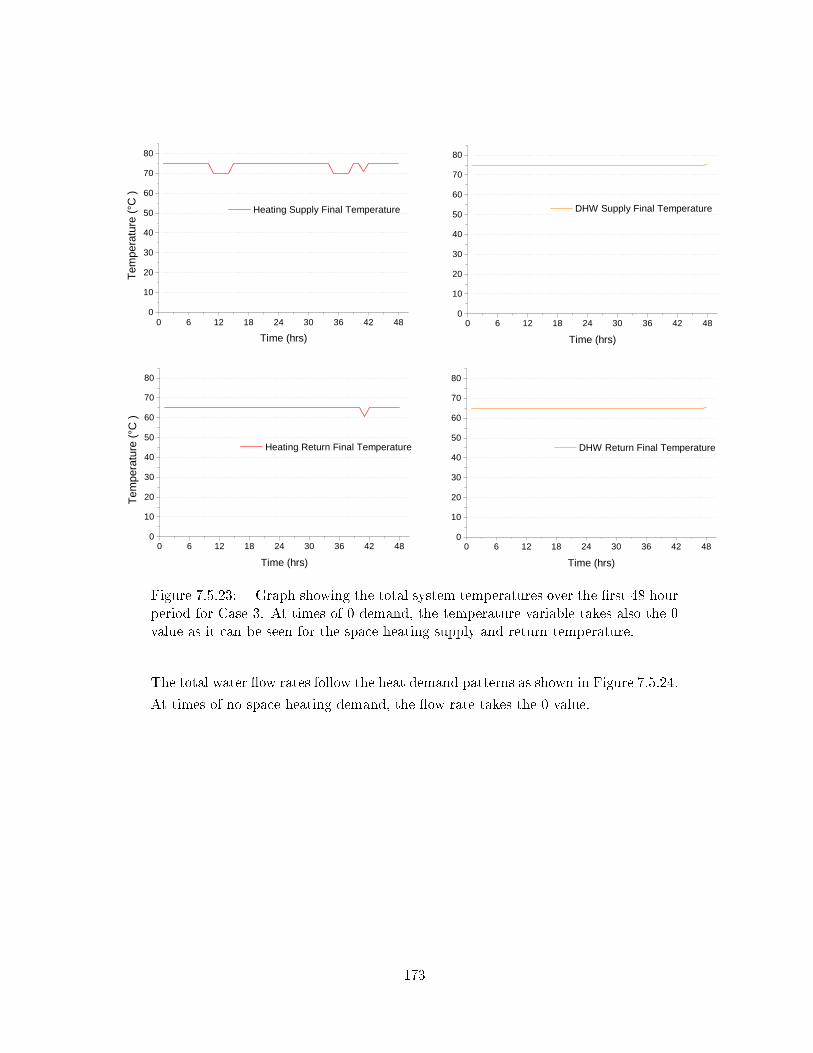
0 6 1 2 1 8 2 4 3 0 3 6 4 2 4 80
1 02 03 04 05 06 07 08 0
H e a t i n g S u p p l y F i n a l T e m p e r a t u r e
Temp
eratur
e (°C
)
T i m e ( h r s )0 6 1 2 1 8 2 4 3 0 3 6 4 2 4 8
01 02 03 04 05 06 07 08 0
D H W S u p p l y F i n a l T e m p e r a t u r e
T i m e ( h r s )
0 6 1 2 1 8 2 4 3 0 3 6 4 2 4 80
1 02 03 04 05 06 07 08 0
H e a t i n g R e t u r n F i n a l T e m p e r a t u r e
Temp
eratur
e (°C
)
T i m e ( h r s )0 6 1 2 1 8 2 4 3 0 3 6 4 2 4 8
01 02 03 04 05 06 07 08 0
D H W R e t u r n F i n a l T e m p e r a t u r e
T i m e ( h r s )
Figure 7.5.23: Graph showing the total system temperatures over the �rst 48 hourperiod for Case 3. At times of 0 demand, the temperature variable takes also the 0value as it can be seen for the space heating supply and return temperature.
The total water �ow rates follow the heat demand patterns as shown in Figure 7.5.24.
At times of no space heating demand, the �ow rate takes the 0 value.
173
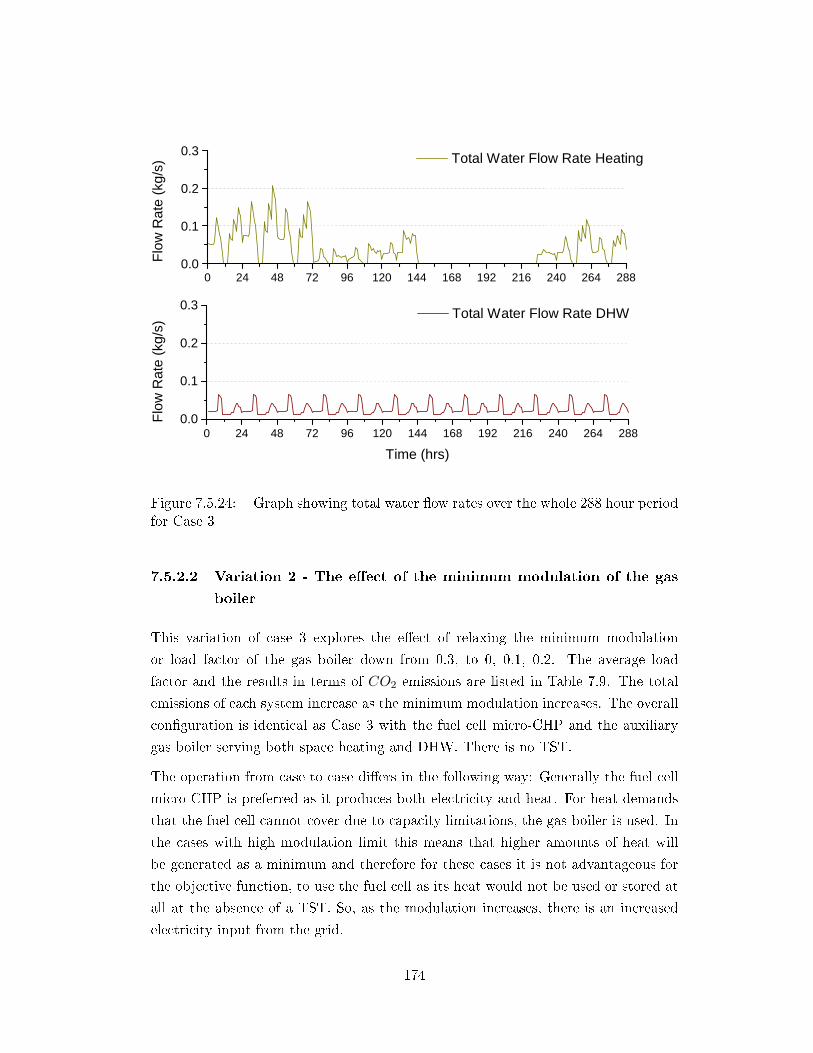
0 2 4 4 8 7 2 9 6 1 2 0 1 4 4 1 6 8 1 9 2 2 1 6 2 4 0 2 6 4 2 8 80 . 0
0 . 1
0 . 2
0 . 3 T o t a l W a t e r F l o w R a t e H e a t i n gFlo
w Rate
(kg/s
)
0 2 4 4 8 7 2 9 6 1 2 0 1 4 4 1 6 8 1 9 2 2 1 6 2 4 0 2 6 4 2 8 80 . 0
0 . 1
0 . 2
0 . 3 T o t a l W a t e r F l o w R a t e D H W
Flow R
ate (k
g/s)
T i m e ( h r s )
Figure 7.5.24: Graph showing total water �ow rates over the whole 288 hour periodfor Case 3
7.5.2.2 Variation 2 - The e�ect of the minimum modulation of the gas
boiler
This variation of case 3 explores the e�ect of relaxing the minimum modulation
or load factor of the gas boiler down from 0.3, to 0, 0.1, 0.2. The average load
factor and the results in terms of CO2 emissions are listed in Table 7.9. The total
emissions of each system increase as the minimum modulation increases. The overall
con�guration is identical as Case 3 with the fuel cell micro-CHP and the auxiliary
gas boiler serving both space heating and DHW. There is no TST.
The operation from case to case di�ers in the following way: Generally the fuel cell
micro-CHP is preferred as it produces both electricity and heat. For heat demands
that the fuel cell cannot cover due to capacity limitations, the gas boiler is used. In
the cases with high modulation limit this means that higher amounts of heat will
be generated as a minimum and therefore for these cases it is not advantageous for
the objective function, to use the fuel cell as its heat would not be used or stored at
all at the absence of a TST. So, as the modulation increases, there is an increased
electricity input from the grid.
174
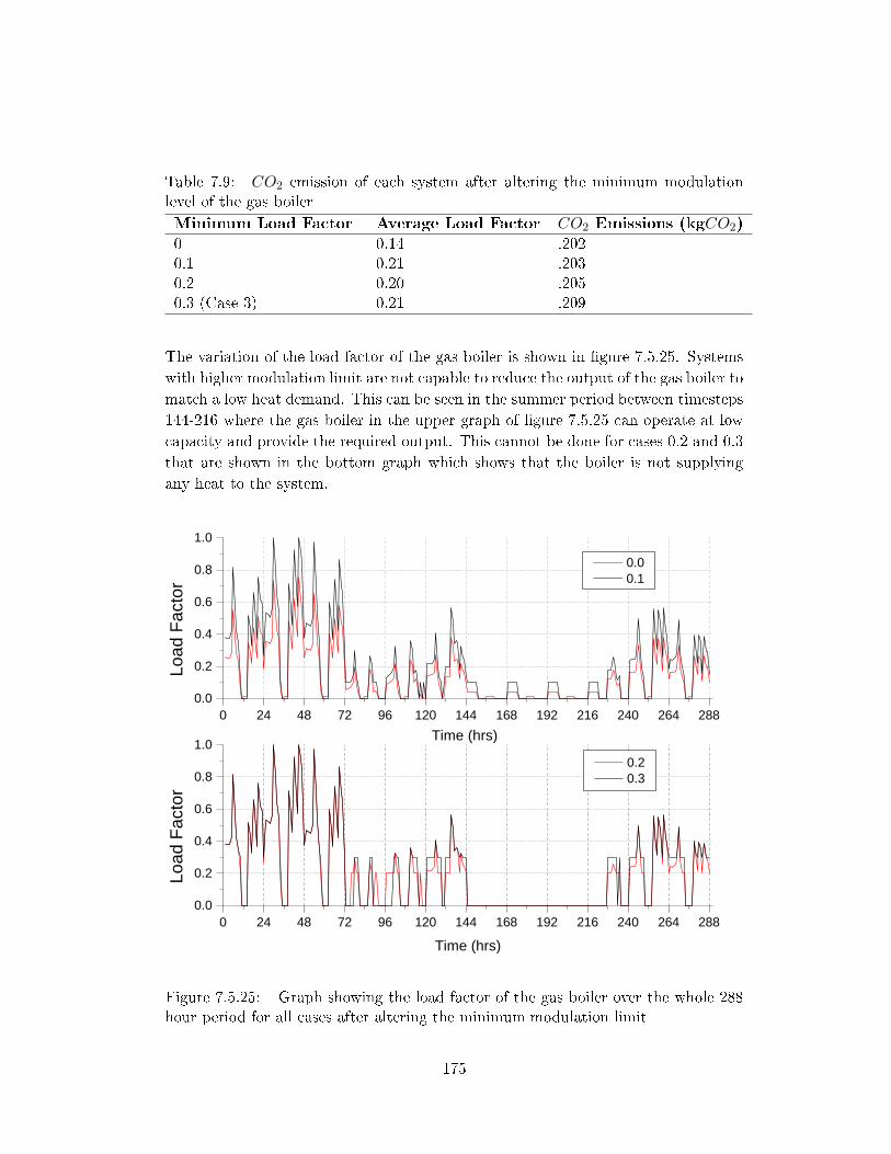
Table 7.9: CO2 emission of each system after altering the minimum modulationlevel of the gas boilerMinimum Load Factor Average Load Factor CO2 Emissions (kgCO2)
0 0.14 .2020.1 0.21 .2030.2 0.20 .2050.3 (Case 3) 0.21 .209
The variation of the load factor of the gas boiler is shown in �gure 7.5.25. Systemswith higher modulation limit are not capable to reduce the output of the gas boiler tomatch a low heat demand. This can be seen in the summer period between timesteps144-216 where the gas boiler in the upper graph of �gure 7.5.25 can operate at lowcapacity and provide the required output. This cannot be done for cases 0.2 and 0.3that are shown in the bottom graph which shows that the boiler is not supplyingany heat to the system.
0 2 4 4 8 7 2 9 6 1 2 0 1 4 4 1 6 8 1 9 2 2 1 6 2 4 0 2 6 4 2 8 80 . 00 . 20 . 40 . 60 . 81 . 0
0 . 2 0 . 3
Load
Facto
r
T i m e ( h r s )
0 2 4 4 8 7 2 9 6 1 2 0 1 4 4 1 6 8 1 9 2 2 1 6 2 4 0 2 6 4 2 8 80 . 00 . 20 . 40 . 60 . 81 . 0
Load
Facto
r
T i m e ( h r s )
0 . 0 0 . 1
Figure 7.5.25: Graph showing the load factor of the gas boiler over the whole 288hour period for all cases after altering the minimum modulation limit
175
7.5.2.3 Case 4
The design and performance of a system comprised of a fuel cell micro-CHP, a
gas boiler and a TST coupled with radiators for heat emitters is evaluated in this
example. The addition of TST in this system compared to case 3 gives a system
designed with a larger fuel cell sized at 3.6 kW. A TST sized at 115 L provides heat
to the system, reducing the operation of the gas boiler and allowing the fuel cell to
cover most of the electricity demand minimising electricity import from grid.
In this optimum design, space heating and DHW demand are covered by all possible
sources, the fuel cell cooling circuit, the afterburner, the gas boiler and the TST.
Table 7.10 shows the annual contribution of each heating source to satisfying demand.
The fuel cell totally covers 72% of space heating and 69% of DHW demand and at
the same time the whole electricity demand.
Table 7.10: Annual heat contribution for each source for case 4
Source Space Heating (%) DHW(%)
FC Cooling Circuit 37.0 31.0Afterburner 35.0 38.0Gas Boiler 27.0 29.0TST 1.0 2.0
Figure 7.5.26 zooms in the whole dataset to show the electricity generation of the
fuel cell on a winter and on a summer day. The fuel cell covers the entire electricity
demand of the dwelling. As the electricity is generating electricity in the summer
when space heating demand is low, all heat is used for DHW as it can be seen in
Figure 7.5.29.
176
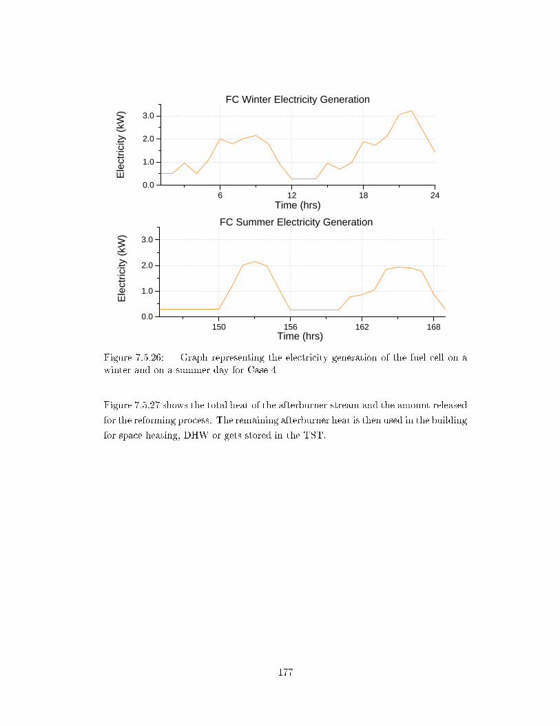
6 1 2 1 8 2 40 . 0
1 . 0
2 . 0
3 . 0
1 5 0 1 5 6 1 6 2 1 6 80 . 0
1 . 0
2 . 0
3 . 0
Electr
icity (
kW)
T i m e ( h r s )
F C W i n t e r E l e c t r i c i t y G e n e r a t i o n
F C S u m m e r E l e c t r i c i t y G e n e r a t i o n
Electr
icity (
kW)
T i m e ( h r s )Figure 7.5.26: Graph representing the electricity generation of the fuel cell on awinter and on a summer day for Case 4
Figure 7.5.27 shows the total heat of the afterburner stream and the amount released
for the reforming process. The remaining afterburner heat is then used in the building
for space heating, DHW or gets stored in the TST.
177
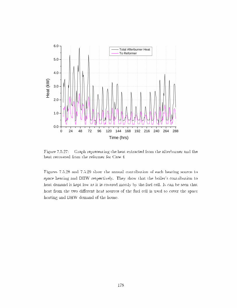
0 2 4 4 8 7 2 9 6 1 2 0 1 4 4 1 6 8 1 9 2 2 1 6 2 4 0 2 6 4 2 8 80 . 0
1 . 0
2 . 0
3 . 0
4 . 0
5 . 0
6 . 0He
at (kW
)
T i m e ( h r s )
T o t a l A f t e r b u r n e r H e a t T o R e f o r m e r
Figure 7.5.27: Graph representing the heat extracted from the afterburner and theheat recovered from the reformer for Case 4
Figures 7.5.28 and 7.5.29 show the annual contribution of each heating source to
space heating and DHW respectively. They show that the boiler's contribution to
heat demand is kept low as it is covered mostly by the fuel cell. It can be seen that
heat from the two di�erent heat sources of the fuel cell is used to cover the space
heating and DHW demand of the house.
178
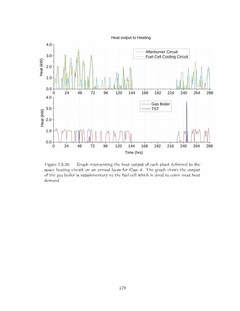
0 2 4 4 8 7 2 9 6 1 2 0 1 4 4 1 6 8 1 9 2 2 1 6 2 4 0 2 6 4 2 8 80 . 0
1 . 0
2 . 0
3 . 0
4 . 0
0 2 4 4 8 7 2 9 6 1 2 0 1 4 4 1 6 8 1 9 2 2 1 6 2 4 0 2 6 4 2 8 80 . 0
1 . 0
2 . 0
3 . 0
4 . 0
A f t e r b u r n e r C i r c u i t F u e l C e l l C o o l i n g C i r c u i t
Heat
(kW)
Heat
(kW)
T i m e ( h r s )
G a s B o i l e r T S T
H e a t o u t p u t t o H e a t i n g
Figure 7.5.28: Graph representing the heat output of each plant delivered to thespace heating circuit on an annual basis for Case 4. The graph shows the outputof the gas boiler is supplementary to the fuel cell which is sized to cover most heatdemand
179
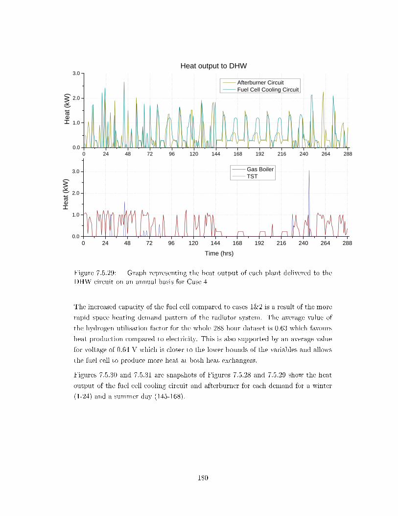
0 2 4 4 8 7 2 9 6 1 2 0 1 4 4 1 6 8 1 9 2 2 1 6 2 4 0 2 6 4 2 8 80 . 0
1 . 0
2 . 0
3 . 0
0 2 4 4 8 7 2 9 6 1 2 0 1 4 4 1 6 8 1 9 2 2 1 6 2 4 0 2 6 4 2 8 80 . 0
1 . 0
2 . 0
3 . 0
A f t e r b u r n e r C i r c u i t F u e l C e l l C o o l i n g C i r c u i t
Heat
(kW)
Heat
(kW)
T i m e ( h r s )
G a s B o i l e r T S T
H e a t o u t p u t t o D H W
Figure 7.5.29: Graph representing the heat output of each plant delivered to theDHW circuit on an annual basis for Case 4
The increased capacity of the fuel cell compared to cases 1&2 is a result of the more
rapid space heating demand pattern of the radiator system. The average value of
the hydrogen utilisation factor for the whole 288 hour dataset is 0.63 which favours
heat production compared to electricity. This is also supported by an average value
for voltage of 0.64 V which is closer to the lower bounds of the variables and allows
the fuel cell to produce more heat at both heat exchangers.
Figures 7.5.30 and 7.5.31 are snapshots of Figures 7.5.28 and 7.5.29 show the heat
output of the fuel cell cooling circuit and afterburner for each demand for a winter
(1-24) and a summer day (145-168).
180
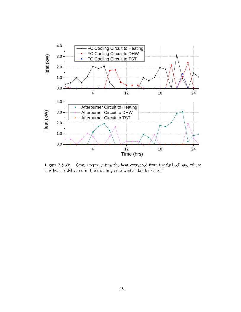
6 1 2 1 8 2 40 . 0
1 . 0
2 . 0
3 . 0
4 . 0
6 1 2 1 8 2 40 . 0
1 . 0
2 . 0
3 . 0
4 . 0
Heat
(kW)
F C C o o l i n g C i r c u i t t o H e a t i n g F C C o o l i n g C i r c u i t t o D H W F C C o o l i n g C i r c u i t t o T S T
Heat
(kW)
T i m e ( h r s )
A f t e r b u r n e r C i r c u i t t o H e a t i n g A f t e r b u r n e r C i r c u i t t o D H W A f t e r b u r n e r C i r c u i t t o T S T
Figure 7.5.30: Graph representing the heat extracted from the fuel cell and wherethis heat is delivered in the dwelling on a winter day for Case 4
181
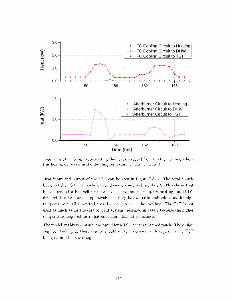
1 5 0 1 5 6 1 6 2 1 6 80 . 0
1 . 0
2 . 0
3 . 0
1 5 0 1 5 6 1 6 2 1 6 80 . 0
1 . 0
2 . 0
Heat
(kW) F C C o o l i n g C i r c u i t t o H e a t i n g
F C C o o l i n g C i r c u i t t o D H W F C C o o l i n g C i r c u i t t o T S T
Heat
(kW)
T i m e ( h r s )
A f t e r b u r n e r C i r c u i t t o H e a t i n g A f t e r b u r n e r C i r c u i t t o D H W A f t e r b u r n e r C i r c u i t t o T S T
Figure 7.5.31: Graph representing the heat extracted from the fuel cell and wherethis heat is delivered in the dwelling on a summer day for Case 4
Heat input and output of the TST can be seen in Figure 7.5.32. The total contri-
bution of the TST in the whole heat demand combined is only 3%. This shows that
for the case of a fuel cell sized to cover a big portion of space heating and DHW
demand, the TST acts supportively ensuring that water is maintained at the high
temperature at all times to be used when needed in the dwelling. The TST is not
used as much as for the case of UFH system presented in case 2 because the higher
temperature required for radiators is more di�cult to achieve.
The model at this case study has opted for a TST that is not used much. The design
engineer looking at these results should make a decision with regard to the TST
being required in the design.
182
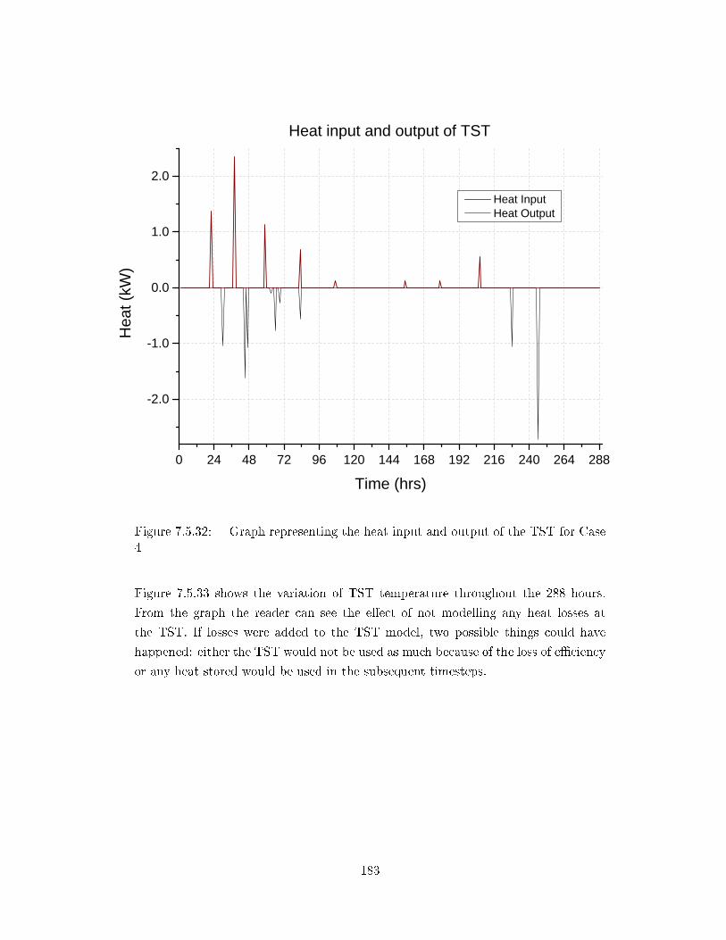
0 2 4 4 8 7 2 9 6 1 2 0 1 4 4 1 6 8 1 9 2 2 1 6 2 4 0 2 6 4 2 8 8
- 2 . 0
- 1 . 0
0 . 0
1 . 0
2 . 0 H e a t I n p u t H e a t O u t p u t
T i m e ( h r s )
Heat
(kW)
H e a t i n p u t a n d o u t p u t o f T S T
Figure 7.5.32: Graph representing the heat input and output of the TST for Case4
Figure 7.5.33 shows the variation of TST temperature throughout the 288 hours.
From the graph the reader can see the e�ect of not modelling any heat losses at
the TST. If losses were added to the TST model, two possible things could have
happened: either the TST would not be used as much because of the loss of e�ciency
or any heat stored would be used in the subsequent timesteps.
183
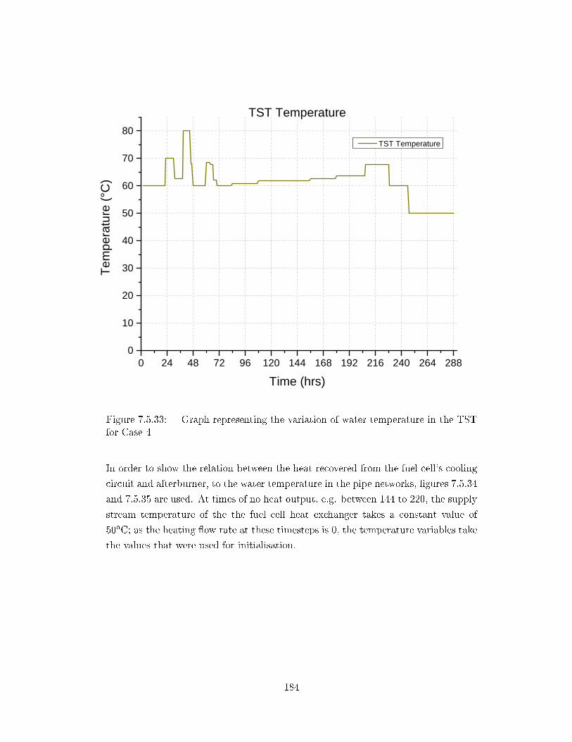
0 2 4 4 8 7 2 9 6 1 2 0 1 4 4 1 6 8 1 9 2 2 1 6 2 4 0 2 6 4 2 8 80
1 0
2 0
3 0
4 0
5 0
6 0
7 0
8 0Te
mpera
ture (
°C)
T i m e ( h r s )
T S T T e m p e r a t u r e
T S T T e m p e r a t u r e
Figure 7.5.33: Graph representing the variation of water temperature in the TSTfor Case 4
In order to show the relation between the heat recovered from the fuel cell's cooling
circuit and afterburner, to the water temperature in the pipe networks, �gures 7.5.34
and 7.5.35 are used. At times of no heat output, e.g. between 144 to 220, the supply
stream temperature of the the fuel cell heat exchanger takes a constant value of
50oC; as the heating �ow rate at these timesteps is 0, the temperature variables take
the values that were used for initialisation.
184
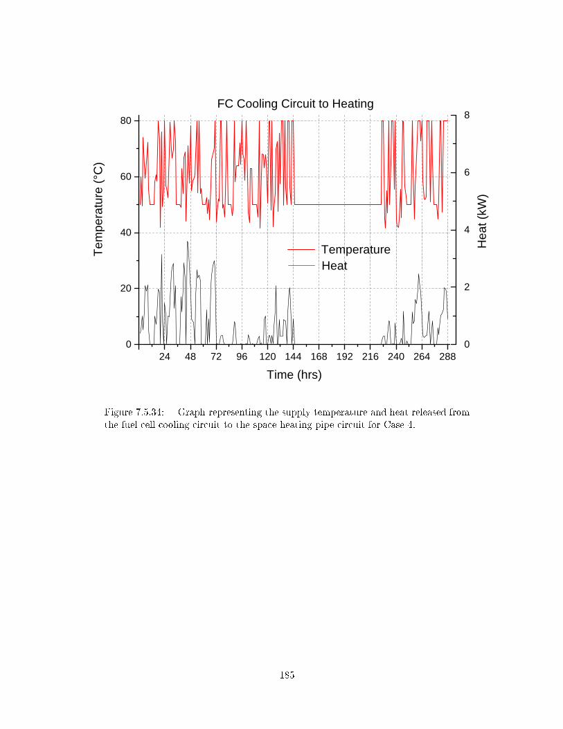
2 4 4 8 7 2 9 6 1 2 0 1 4 4 1 6 8 1 9 2 2 1 6 2 4 0 2 6 4 2 8 80
2 0
4 0
6 0
8 0Te
mpera
ture (
°C)
T i m e ( h r s )
F C C o o l i n g C i r c u i t t o H e a t i n g
T e m p e r a t u r e
0
2
4
6
8
Heat
(kW)
H e a t
Figure 7.5.34: Graph representing the supply temperature and heat released fromthe fuel cell cooling circuit to the space heating pipe circuit for Case 4.
185
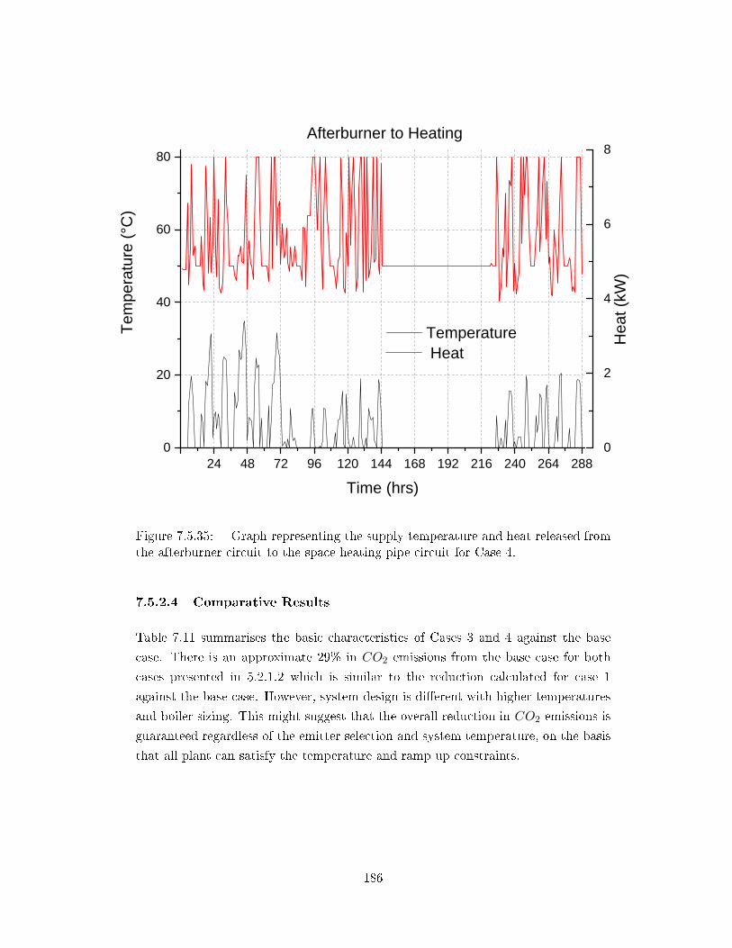
2 4 4 8 7 2 9 6 1 2 0 1 4 4 1 6 8 1 9 2 2 1 6 2 4 0 2 6 4 2 8 80
2 0
4 0
6 0
8 0Te
mpera
ture (
°C)
T i m e ( h r s )
T e m p e r a t u r e
0
2
4
6
8A f t e r b u r n e r t o H e a t i n g
H e a t Heat
(kW)
Figure 7.5.35: Graph representing the supply temperature and heat released fromthe afterburner circuit to the space heating pipe circuit for Case 4.
7.5.2.4 Comparative Results
Table 7.11 summarises the basic characteristics of Cases 3 and 4 against the base
case. There is an approximate 29% in CO2 emissions from the base case for both
cases presented in 5.2.1.2 which is similar to the reduction calculated for case 1
against the base case. However, system design is di�erent with higher temperatures
and boiler sizing. This might suggest that the overall reduction in CO2 emissions is
guaranteed regardless of the emitter selection and system temperature, on the basis
that all plant can satisfy the temperature and ramp up constraints.
186
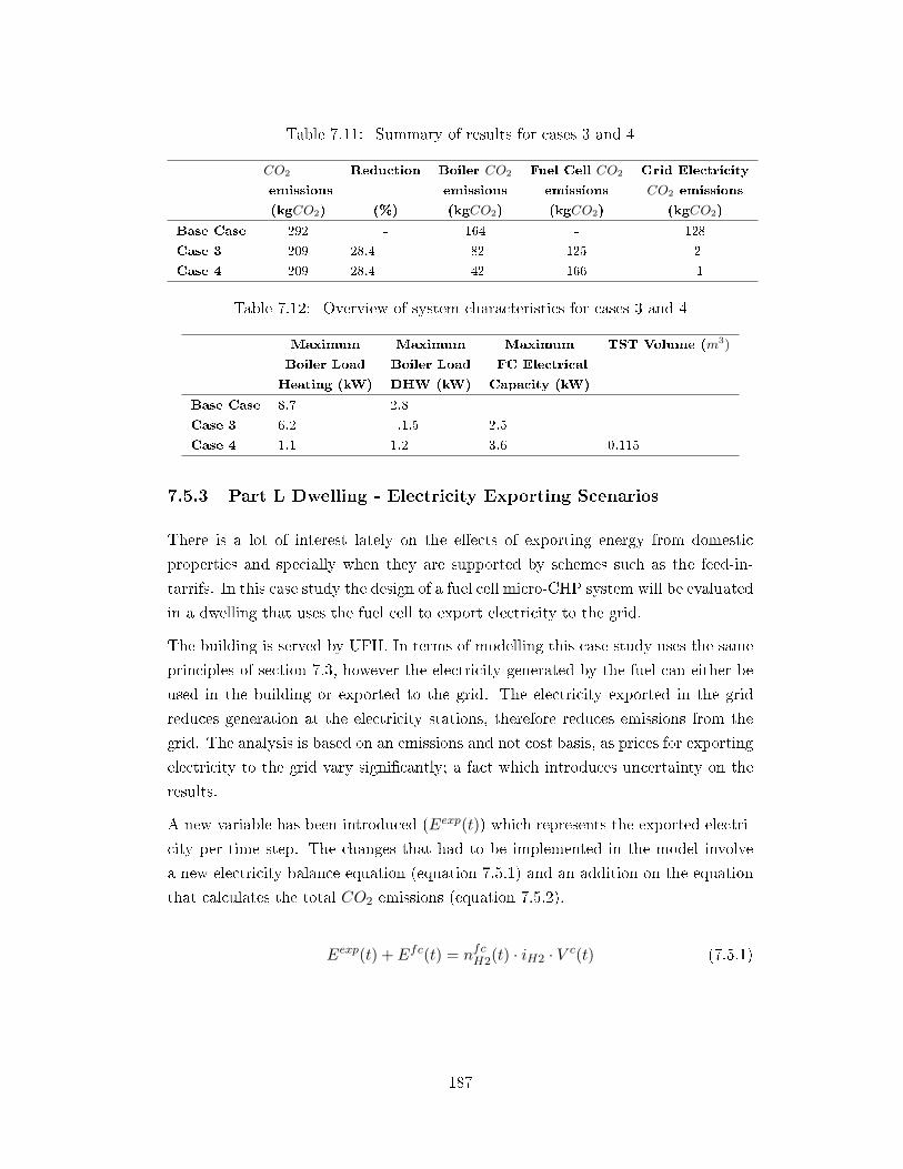
Table 7.11: Summary of results for cases 3 and 4
CO2 Reduction Boiler CO2 Fuel Cell CO2 Grid Electricity
emissions emissions emissions CO2 emissions
(kgCO2) (%) (kgCO2) (kgCO2) (kgCO2)
Base Case 292 - 164 - 128
Case 3 209 28.4 82 125 2
Case 4 209 28.4 42 166 1
Table 7.12: Overview of system characteristics for cases 3 and 4
Maximum Maximum Maximum TST Volume (m3)
Boiler Load Boiler Load FC Electrical
Heating (kW) DHW (kW) Capacity (kW)
Base Case 8.7 2.8 - -
Case 3 6.2 .1.5 2.5 -
Case 4 1.1 1.2 3.6 0.115
7.5.3 Part L Dwelling - Electricity Exporting Scenarios
There is a lot of interest lately on the e�ects of exporting energy from domestic
properties and specially when they are supported by schemes such as the feed-in-
tarrifs. In this case study the design of a fuel cell micro-CHP system will be evaluated
in a dwelling that uses the fuel cell to export electricity to the grid.
The building is served by UFH. In terms of modelling this case study uses the same
principles of section 7.3, however the electricity generated by the fuel can either be
used in the building or exported to the grid. The electricity exported in the grid
reduces generation at the electricity stations, therefore reduces emissions from the
grid. The analysis is based on an emissions and not cost basis, as prices for exporting
electricity to the grid vary signi�cantly; a fact which introduces uncertainty on the
results.
A new variable has been introduced (Eexp(t)) which represents the exported electri-
city per time step. The changes that had to be implemented in the model involve
a new electricity balance equation (equation 7.5.1) and an addition on the equation
that calculates the total CO2 emissions (equation 7.5.2).
Eexp(t) + Efc(t) = nfcH2(t) · iH2 · V c(t) (7.5.1)
187
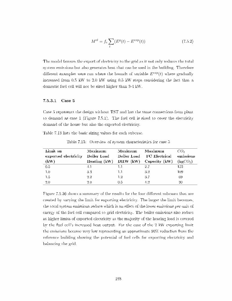
M el = fe∑
(t
Eg(t)− Eexp(t)) (7.5.2)
The model favours the export of electricity to the grid as it not only reduces the total
system emissions but also generates heat that can be used in the building. Therefore
di�erent examples were run where the bounds of variable Eexp(t) where gradually
increased from 0.5 kW to 2.0 kW using 0.5 kW steps considering the fact that a
domestic fuel cell will not be sized higher than 3-4 kW.
7.5.3.1 Case 5
Case 5 represents the design without TST and has the same connections from plant
to demand as case 1 (Figure 7.5.1). The fuel cell is sized to cover the electricity
demand of the house but also the exported electricity.
Table 7.13 lists the basic sizing values for each subcase.
Table 7.13: Overview of system characteristics for case 5
Limit on Maximum Maximum Maximum CO2
exported electricity Boiler Load Boiler Load FC Electrical emissions
(kW) Heating (kW) DHW (kW) Capacity (kW) (kgCO2)
0.5 4.1 1.1 2.7 152
1.0 3.3 1.1 3.2 109
1.5 2.2 1.2 3.7 69
2.0 2.0 0.5 4.2 30
Figure 7.5.36 shows a summary of the results for the four di�erent subcases that are
created by varying the limit for exporting electricity. The larger the limit becomes,
the total system emissions reduce which is an e�ect of the lower emissions per unit of
energy of the fuel cell compared to grid electricity. The boiler emissions also reduce
at higher limits of exported electricity as the majority of the heating load is covered
by the fuel cell's increased heat output. For the case of the 2 kW exporting limit
the emissions become very low representing an approximate 90% reduction from the
reference building showing the potential of fuel cells for exporting electricity and
balancing the grid.
188

0 . 5 k W E X P
1 k W E X P
1 . 5 k W E X P
2 k W E X P
- 3 0 0 - 2 0 0 - 1 0 0 0 1 0 0 2 0 0 3 0 0C O 2 E m i s s i o n s ( k g C O 2 )
T o t a l E m i s s i o n s F u e l C e l l E m i s s i o n s B o i l e r e m i s s i o n s G r i d E l e c t r i c i t y E m i s s i o n s E l e c t r i c i t y E x p o r t E m i s s i o n s
Figure 7.5.36: Breakdown of emissions caused by altering the limit of exportedelectricity to the grid for case 5. Emissions reduce as the limit increases
7.5.3.2 Case 6
The case that incorporates a TST the extreme case of 2 kW exporting limit was
looked at as it represented the case with the highest savings. The inclusion of thermal
storage in Case 6 gives an approximate 8% reduction of total emissions compared
to case 5. For the 2 kW limit on electricity export the emissions reduce from 30.4
kgCO2 to to 28.0 kgCO2 with the main system characteristics shown on Table 7.14.
Table 7.14: Overview of system characteristics for case 6
Limit on Maximum Maximum Maximum TST CO2
exported Boiler Load Boiler Load FC Electrical Volume emissions
electricity (kW) Heating (kW) DHW (kW) Capacity (kW) (m3) (kgCO2)
2.0 0.8 0.2 4.2 0.343 28.0
189
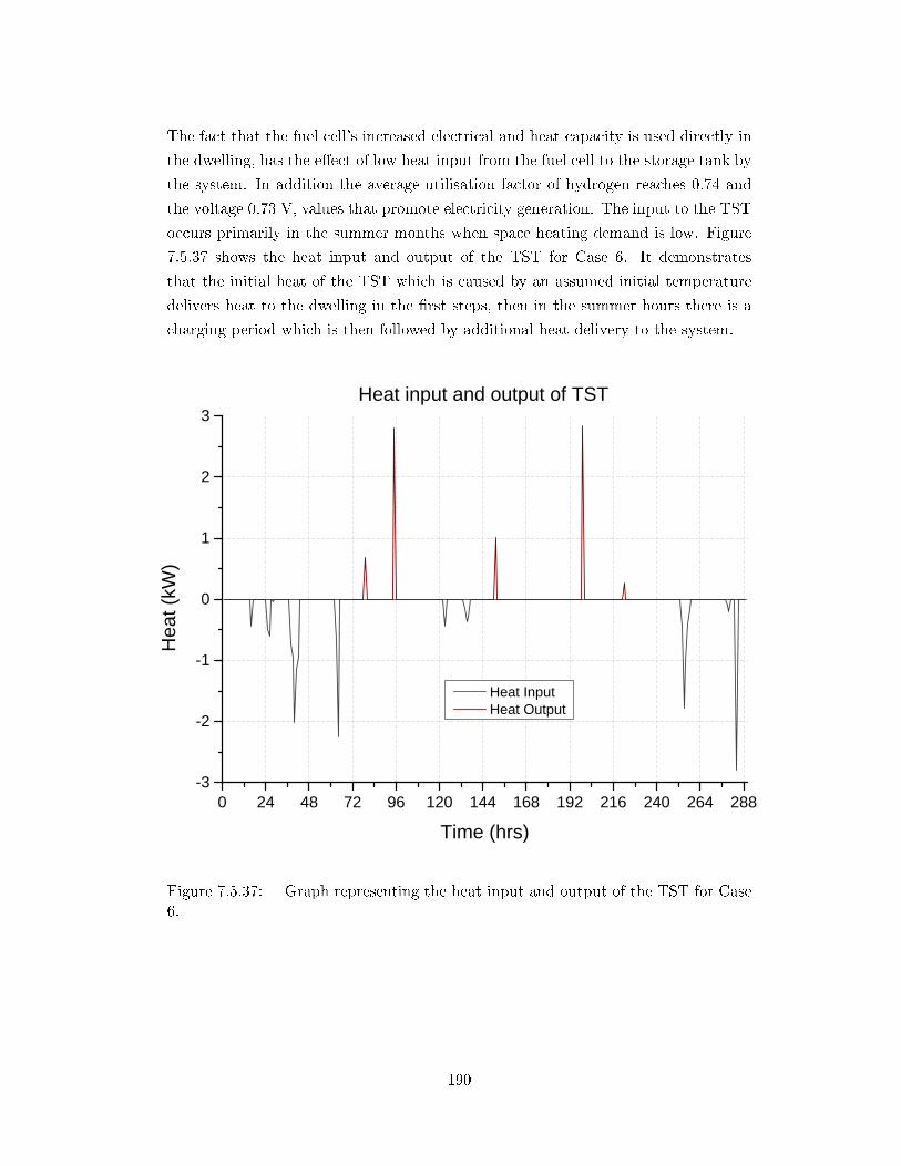
The fact that the fuel cell's increased electrical and heat capacity is used directly in
the dwelling, has the e�ect of low heat input from the fuel cell to the storage tank by
the system. In addition the average utilisation factor of hydrogen reaches 0.74 and
the voltage 0.73 V, values that promote electricity generation. The input to the TST
occurs primarily in the summer months when space heating demand is low. Figure
7.5.37 shows the heat input and output of the TST for Case 6. It demonstrates
that the initial heat of the TST which is caused by an assumed initial temperature
delivers heat to the dwelling in the �rst steps, then in the summer hours there is a
charging period which is then followed by additional heat delivery to the system.
0 2 4 4 8 7 2 9 6 1 2 0 1 4 4 1 6 8 1 9 2 2 1 6 2 4 0 2 6 4 2 8 8- 3
- 2
- 1
0
1
2
3
H e a t I n p u t H e a t O u t p u t
T i m e ( h r s )
Heat
(kW)
H e a t i n p u t a n d o u t p u t o f T S T
Figure 7.5.37: Graph representing the heat input and output of the TST for Case6.
190
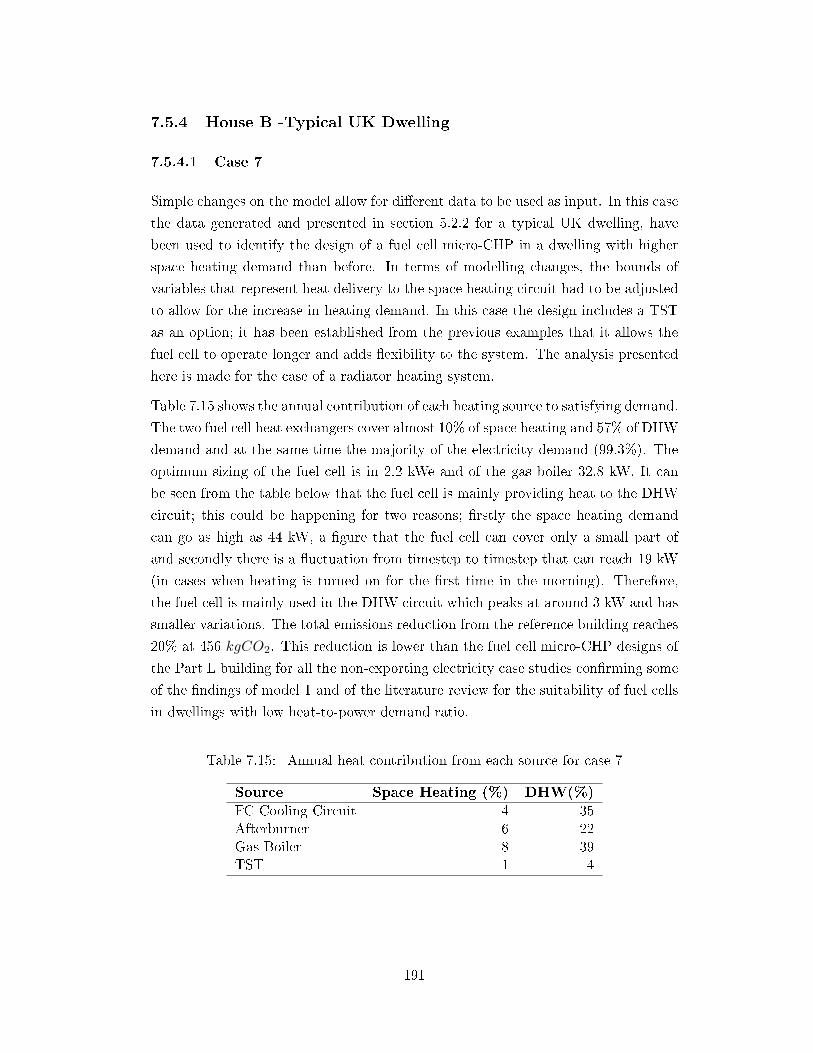
7.5.4 House B -Typical UK Dwelling
7.5.4.1 Case 7
Simple changes on the model allow for di�erent data to be used as input. In this case
the data generated and presented in section 5.2.2 for a typical UK dwelling, have
been used to identify the design of a fuel cell micro-CHP in a dwelling with higher
space heating demand than before. In terms of modelling changes, the bounds of
variables that represent heat delivery to the space heating circuit had to be adjusted
to allow for the increase in heating demand. In this case the design includes a TST
as an option; it has been established from the previous examples that it allows the
fuel cell to operate longer and adds �exibility to the system. The analysis presented
here is made for the case of a radiator heating system.
Table 7.15 shows the annual contribution of each heating source to satisfying demand.
The two fuel cell heat exchangers cover almost 10% of space heating and 57% of DHW
demand and at the same time the majority of the electricity demand (99.3%). The
optimum sizing of the fuel cell is in 2.2 kWe and of the gas boiler 32.8 kW. It can
be seen from the table below that the fuel cell is mainly providing heat to the DHW
circuit; this could be happening for two reasons; �rstly the space heating demand
can go as high as 44 kW, a �gure that the fuel cell can cover only a small part of
and secondly there is a �uctuation from timestep to timestep that can reach 19 kW
(in cases when heating is turned on for the �rst time in the morning). Therefore,
the fuel cell is mainly used in the DHW circuit which peaks at around 3 kW and has
smaller variations. The total emissions reduction from the reference building reaches
20% at 456 kgCO2. This reduction is lower than the fuel cell micro-CHP designs of
the Part L building for all the non-exporting electricity case studies con�rming some
of the �ndings of model 1 and of the literature review for the suitability of fuel cells
in dwellings with low heat-to-power demand ratio.
Table 7.15: Annual heat contribution from each source for case 7
Source Space Heating (%) DHW(%)
FC Cooling Circuit 4 35Afterburner 6 22Gas Boiler 8 39TST 1 4
191
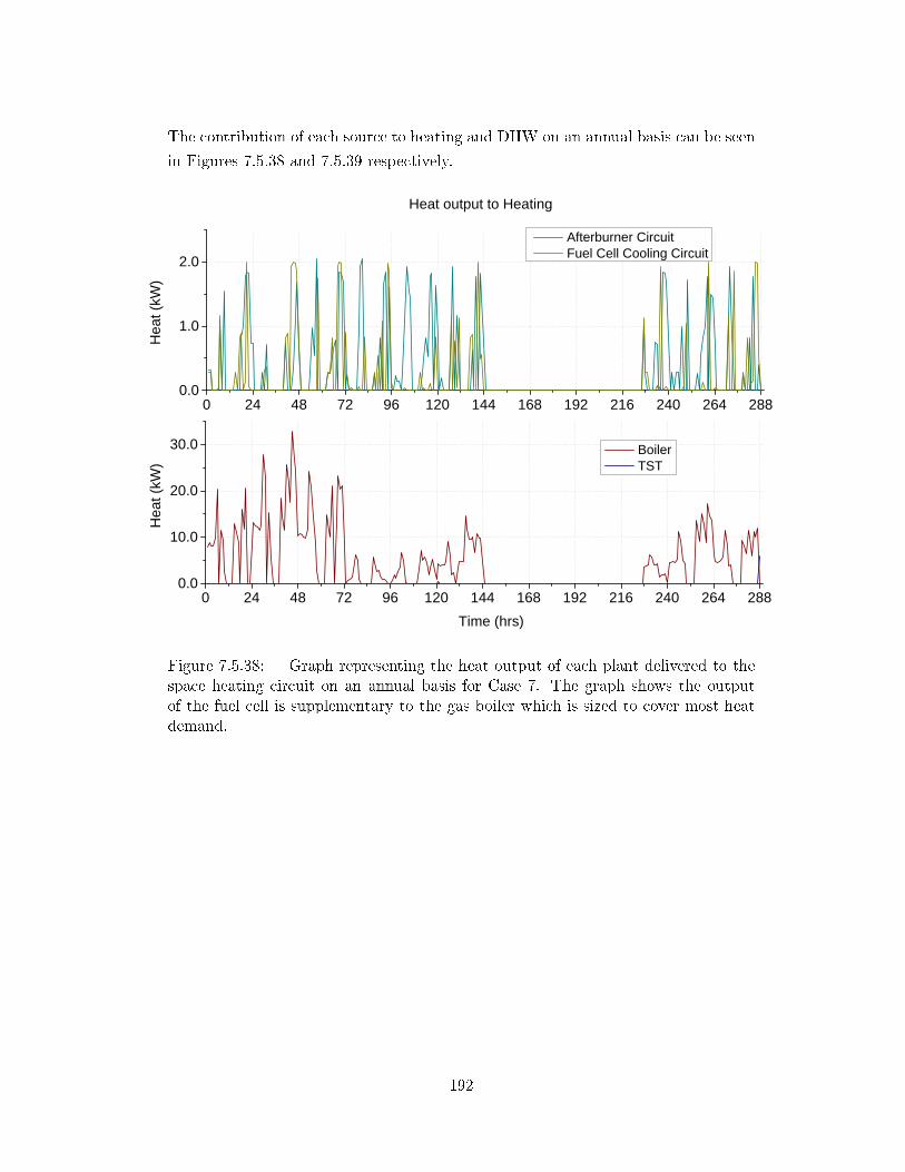
The contribution of each source to heating and DHW on an annual basis can be seen
in Figures 7.5.38 and 7.5.39 respectively.
0 2 4 4 8 7 2 9 6 1 2 0 1 4 4 1 6 8 1 9 2 2 1 6 2 4 0 2 6 4 2 8 80 . 0
1 . 0
2 . 0
0 2 4 4 8 7 2 9 6 1 2 0 1 4 4 1 6 8 1 9 2 2 1 6 2 4 0 2 6 4 2 8 80 . 0
1 0 . 0
2 0 . 0
3 0 . 0
A f t e r b u r n e r C i r c u i t F u e l C e l l C o o l i n g C i r c u i t
Heat
(kW)
Heat
(kW)
T i m e ( h r s )
B o i l e r T S T
H e a t o u t p u t t o H e a t i n g
Figure 7.5.38: Graph representing the heat output of each plant delivered to thespace heating circuit on an annual basis for Case 7. The graph shows the outputof the fuel cell is supplementary to the gas boiler which is sized to cover most heatdemand.
192
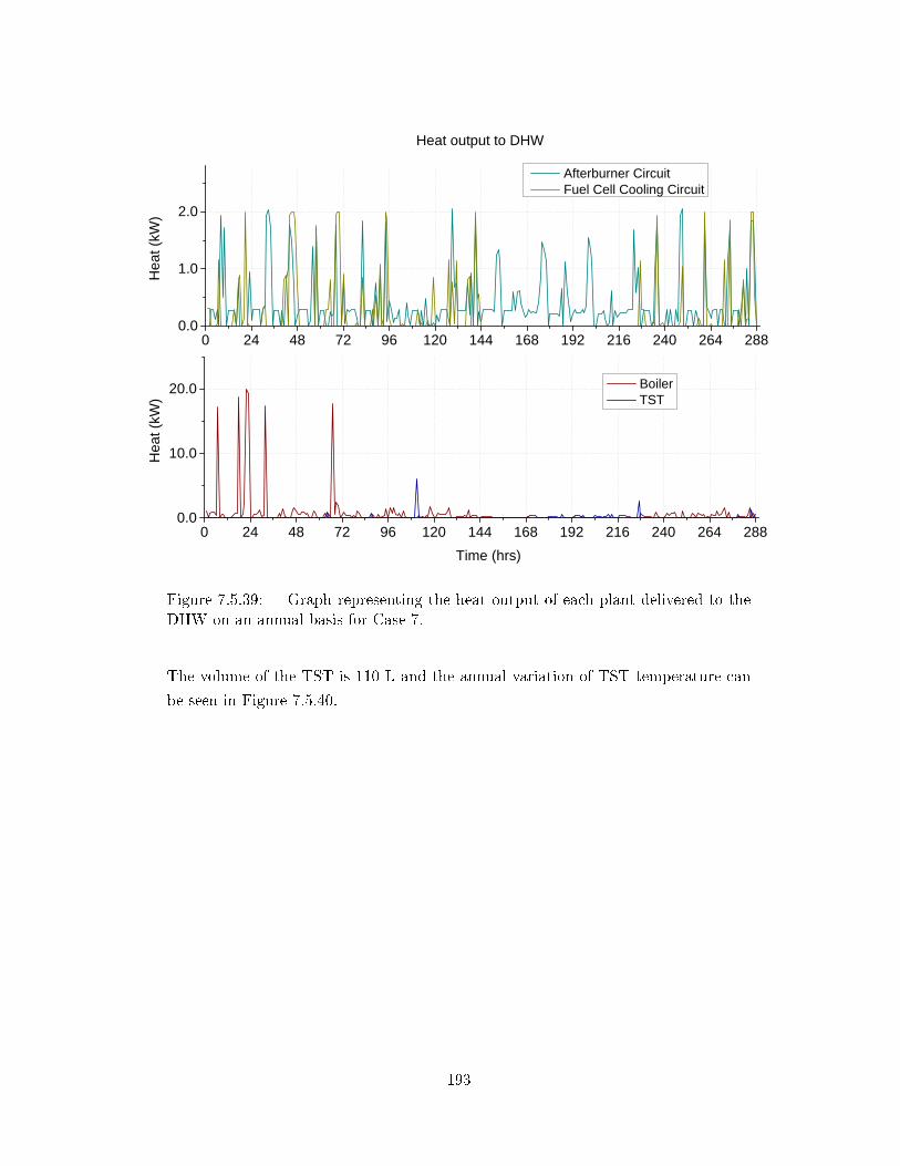
0 2 4 4 8 7 2 9 6 1 2 0 1 4 4 1 6 8 1 9 2 2 1 6 2 4 0 2 6 4 2 8 80 . 0
1 . 0
2 . 0
0 2 4 4 8 7 2 9 6 1 2 0 1 4 4 1 6 8 1 9 2 2 1 6 2 4 0 2 6 4 2 8 80 . 0
1 0 . 0
2 0 . 0
A f t e r b u r n e r C i r c u i t F u e l C e l l C o o l i n g C i r c u i t
Heat
(kW)
Heat
(kW)
T i m e ( h r s )
B o i l e r T S T
H e a t o u t p u t t o D H W
Figure 7.5.39: Graph representing the heat output of each plant delivered to theDHW on an annual basis for Case 7.
The volume of the TST is 110 L and the annual variation of TST temperature can
be seen in Figure 7.5.40.
193
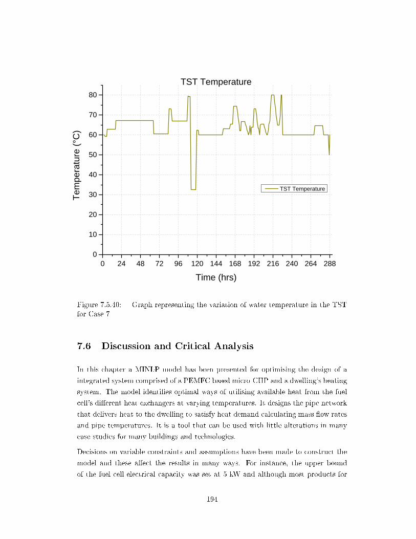
0 2 4 4 8 7 2 9 6 1 2 0 1 4 4 1 6 8 1 9 2 2 1 6 2 4 0 2 6 4 2 8 80
1 0
2 0
3 0
4 0
5 0
6 0
7 0
8 0Te
mpera
ture (
°C)
T i m e ( h r s )
T S T T e m p e r a t u r e
T S T T e m p e r a t u r e
Figure 7.5.40: Graph representing the variation of water temperature in the TSTfor Case 7
7.6 Discussion and Critical Analysis
In this chapter a MINLP model has been presented for optimising the design of a
integrated system comprised of a PEMFC based micro-CHP and a dwelling's heating
system. The model identi�es optimal ways of utilising available heat from the fuel
cell's di�erent heat exchangers at varying temperatures. It designs the pipe network
that delivers heat to the dwelling to satisfy heat demand calculating mass �ow rates
and pipe temperatures. It is a tool that can be used with little alterations in many
case studies for many buildings and technologies.
Decisions on variable constraints and assumptions have been made to construct the
model and these a�ect the results in many ways. For instance, the upper bound
of the fuel cell electrical capacity was set at 5 kW and although most products for
194
domestic micro-generation applications are sized at smaller capacity, this allows the
model to provide unconstrained results for this variable. This is true for case 4 where
a higher capacity than most cases 3.6 kW fuel cell has been selected. Similarly, the
method for modelling the TST tank also determines how much it is being used.
The variation of Case 2 that was run with a di�erent modelling approach presents
a system that relies more on the boiler and uses less the TST. Also, the constraint
imposed on the minimum modulation of the gas boiler de�nes the system operation
as it was shown in 7.5.2.2.
The concept of using data from BIM software as input of the models provides bene�ts
compared to other studies which don't use building data at all [90] or use assumed
�gures for energy demand per season [13]. The use of simulated data of two extremes
in terms of energy demand provides a de�ned basis for understanding the results.
The choice of objective function de�nes the results of the model. In this case the
results obtained minimise CO2, while many researchers have selected to minimise
cost. In terms of system sizing the optimum electrical capacity of the fuel cell is
generally higher than most studies in literature and that can be considered an e�ect
of the choice of the objective function. Hawkes et al. calculated an optimum fuel
cell capacity between 0.9 kW and 1.3 kW by using cost as the objective function
[73]. In terms of system operation and energy outputs, Napoli et al. performed both
energy and economic analysis for fuel cell micro-CHP systems and found out that
following the electrical demand pro�le is preferable in terms of energy and cost, as
it increases the independence of the systems from the grid [93]. This is something
that is demonstrated here as well as for most con�gurations examined, the fuel cell
operation is electricity led with the majority of electricity (above 90% for all cases)
covered by the fuel cell. The electrical led mode is easier to be followed by the fuel
cell compared to the thermal because of its lower primary energy consumption. The
thermal load pro�le is generally higher compared to the fuel cell capacity as also
discussed by [93]. However case 4 which is a dwelling heated by radiators showed
that a fuel cell sized higher compared to all other (non-exporting electricity) case
studies can satisfy a big portion of the space heating demand. Generally for all
con�gurations the fuel cell micro-CHP has the priority in operation and all the other
systems around it run supportively. The UK Good Practice Guide 388 Combined
heat and power for buildings suggests that regardless of the connection method, the
CHP should operate as the lead boiler in order to maximise its operating hours. [1].
This is something shown in the results especially for the systems with TST which
extend the fuel cell's operating hours.
The comparison between the system design for slower heating systems such as UFH
195
and for systems with radiators suggests that the fuel cell system can handle easier
the smooth demand pattern of the UFH system and covers a higher percentage of
the demand. This is because of the ramp up rate constraints of the fuel cell and of
the amount of heat demand which becomes higher than the fuel cell capacity.
Thermal storage increases predicted CO2 savings compared to the cases without
storage. Its inclusion in the design and the correct sizing reduces the use of gas
boiler and grid electricity allowing the fuel cell to operate more hours. When the
thermal and electrical demand pro�les follow di�erent patterns, the additional heat
produced by the fuel cell can be stored in a thermal storage tank. Storage tanks of
larger volume are preferred on low temperature UFH systems while smaller tanks
that be charged and achieve a higher 60-80oC temperature are preferred for radiator
systems. Barbieri et al. [18] makes a similar point concluding that the e�ect that the
size of the thermal energy storage has on the system, is not linearly correlated to the
power of the fuel cell but it is system speci�c. Bianchi et al. concludes that �...the
analysis of the energy performance shows that CHP units, with an appropriately
sized thermal storage system, can cover the overall thermal energy demand with a
primary energy saving index ranging from about 15�45%, depending on the CHP
technology.�[23]. This is true for all case studies with more than 25% emissions
reductions from the reference cases. The optimum size of plant however has also
space constraints that can in�uence the decision of inclusion of a fuel cell micro-
CHP into a dwelling, aside from any environmental or cost bene�ts. A bigger plant
room than typically required for conventional systems is needed to accommodate the
micro-CHP unit, the auxiliary boiler, the TST and all supportive systems.
The utilisation factor of hydrogen and voltage can act as a controlling measure of
the fuel cell: when Ufc and voltage reduce, less electricity is produced at the fuel
cell and more heat can be recovered from the afterburner as more hydrogen will be
combusted. In the summer when less heat is required than the winter period, the
utilisation factor takes values closer to its higher bound to maintain a high electricity
output and to the reduce heat output.
In cases of high electricity demand covered by the fuel cell micro-CHP, there is surplus
thermal energy which can be recovered in the TST. This generates the potential to
increase the e�ciency of the system as boiler use will be reduced. The exporting
electricity case studies show that the electricity exported to the grid has a high
impact on the results, both in terms of outputs and sizing of plant, in allexporting
limits. This can be justi�ed by the e�ect of exporting electricity on the objective
function which is signi�cant.
Barbieri [19] in a study that examined various micro-CHP technologies concluded
196
that the suitability of a micro-CHP technology in a dwelling increases when the
power to heat ratio of the unit �ts the power to heat ratio of the demand. This point
is con�rmed in this study as the case study that presented the typical UK dwelling
appears to have lower reduction in emissions compared to the case studies for House
A. The in�uence of the energy e�ciency of the house on system performance has
been studied by Gandiglio et al. [68]. In their study, in a high e�ciency building,
the PEMFC stack cogeneration heat can satisfy the thermal load required for the
household. On the contrary PEMFC stacks on lower class buildings are able to
provide only 20% of the required thermal power. Similar �ndings occur in case 7 on
a typical UK dwelling where the fuel cell stack is only able to provide a 10% of the
space heating demand.
The minimum modulation limit of plant has been found to a�ect the total system op-
eration and emissions. Di�erent boiler manufacturers produce models with di�erent
characteristics and a boiler that has a low modulation limit can increase predicted
CO2 savings by being able to generate the exact amount of heat required in an
instance.
The higher heating value has been used for this model to represent the heat generated
from combustion of methane in the case of the gas boiler and hydrogen in the case
of the fuel cell micro-CHP afterburner. However this assumption is not accurate
for all timesteps as it depends on the system return temperature. According to the
micro-CHP accelerator report by Carbon Trust �a condensing boiler will only operate
in condensing mode with a water return temperature of 57ºC or below and needs
this to fall nearer to 50ºC for signi�cant condensation� [32]. For the majority of the
cases examined the average return temperature of the system is below 60 oC, so both
systems will have a good enough representation of the extra energy from condensing
the generated exhaust gases vapour.
Stack degradation which occurs for a fuel cell at a rate of 1�2 μV·h can increase with
load cycling, start�stop cycles, low humidity at the stack, temperatures above 90 °C
and lack of fuel in the anode [41]. In all cases presented here, the fuel cell operates at
all times, generating the majority of electricity, so there are no start-stop cycles and
no fuel starvation of the stack. The summer heat demand for DHW is the reason
these problems are avoided as the fuel cell micro-CHP heat can be used for hot water
generation.
The extra level of detail compared to other similar studies that becomes available as
the model's output is the temperature and �ow rates at the heat exchangers of the fuel
cell micro-CHP system. This allows manufacturers and designers to size the micro-
CHP heat exchangers. Also with the available information on temperature and �ow
197
rates, the heating and DHW network pipework can be sized and an approximation of
the circulation pump's capacity can be obtained. This information will help building
services designers choose the �nalised pipework circuits. These circuits may include
compensated heating circuits: The decision to include a three port valve in the
heating circuit after the main heating header is something that can be determined
because the exact variation of �ow temperature is known.
The fuel cell stack temperature de�nes the cooling water temperature which will
be used in the dwelling. In the few studies in literature that the heating system
temperature constraints are taken into account, the stack and exhaust temperatures
are assumed to be constant at a certain level. Gandiglio et al. have assumed a stack
temperature and afterburner exhaust of 62 oC and 120 oC respectively [68]. The
model in this thesis uses an optimisation framework and allows a varying temperature
at the cooling and afterburner exhaust circuits obtained at the results. The varying
�ow rate and temperature at the heating and DHW circuits de�ne the amount of
heat that can be captured.
The novelty of this model is that it considers the plant and house as one and optimises
the whole system designing plant and heating pipework. The inclusion of temperat-
ure and �ow rates for the di�erent process streams within the fuel cell micro-CHP
and the dwelling's space heating and DHW circuits provide a design solution.
7.7 Limitations of the study
An element that the model lacks is the consideration of the policy drivers and sub-
sequent cost reductions behind the commercialisation of the fuel cell micro-CHP. The
feed-in-tarrifs and the impact of di�erent support schemes can contribute on improv-
ing the cost of micro-CHP units. These drivers can be integrated in the model by
introducing a cost function as the objective function.
Another limitation of this study is related to the temporal precision of the model
which is in hourly timesteps. The minute by minute variability of power and heat
demand cannot be captured in hourly data, therefore the results carry the assumption
of a constant load within this hourly timestep. The peaks in energy demand that
occur usually for a short amount of time are averaged in the 1-hour period. A model
based on a 5-minute timestep run for a few hours would capture the variations in
electricity and heat demand that occur in this shorter period. The fuel cell micro-
CHP and all plant would have to respond to these demands and that could uncover
their limitations in terms of ramping up or down. In timesteps that e.g. a 50%
198
increase in the electricity demand occurs that cannot be satis�ed by the fuel cell,
grid electricity will be used. This element cannot be captured by models using
hourly timesteps. A small case study on 5-minute timesteps could be run on selected
designs after the entire 288-hour model has been run, as a robustness test. Despite
this limitation, the bene�t of a yearly dataset is that it can capture the seasonal
variation of all demands and deliver a design that can satisfy them.
The same limitations discussed for the TST model presented in Chapter 6 occur here
because no heat losses are considered in the TST and in pipework. In addition, the
e�ect of the initial energy levels of the TST in the results was raised as an issue that
was addressed in di�erent ways in the model.
7.8 Concluding Remarks
In this Chapter, a MINLP model formulation has been presented for designing a fuel
cell micro-CHP in dwellings optimising the resulting CO2 emissions from the whole
dwelling energy system. The model considers the variability of the di�erent heating
systems and their temperature constraints while at the same time it utilises di�erent
sources of heat from the fuel cell heat exchangers and other plant of the design to
match thermal demand.
199
Chapter 8
Conclusions and Future Directions
The aim of this thesis was to provide tools for designing fuel cell micro-CHP systems
for domestic applications. Towards that goal, a number of mathematical models
were developed and their results were presented in the previous chapters. In the
following section, the main contributions of the thesis are summarised followed by
new directions for future work.
8.1 Summary of Contribution
This thesis focused on the optimisation of fuel cell micro-CHP systems design in
dwellings. In Chapter 1, some basic background information were presented followed
by the aims and objectives of this project. In Chapter 2 the context of the project
was presented focusing on the UK energy market, fuel cell design and products, the
built environment and �nally the design of heating systems.
In Chapter 3, current approaches in the area of fuel cell micro-CHP modelling were
highlighted. Most current models of fuel cell micro-CHP in dwellings ignore the
building side of the system when evaluating the performance of the system or con-
ducting a techno-economical assessment. An element missing from existing models
in literature is related to the temperature constraints of the various heat sources
and distribution systems and how these can be integrated into a reliable system that
can satisfy the varying energy demand of a dwelling. At the same time as fuel cells
do not represent a technology that is established in the micro-generation market,
their potential savings in the domestic energy sector are not very well understood
yet. Based on the �ndings of the literature, chapter presented the options of heat
recovery in fuel cells. It mentioned the need for a systematic modelling tool for
200
designing such systems. There is potential for energy savings from understanding
and applying the results of optimisation models that consider the various heat ex-
changers of the fuel cell micro-CHP and the building services of the dwelling. The
next chapter presented the modelling process in BIM software that provided energy
demand data for a dwelling and also the reference building that all the models can
be compared against. In Chapter 6 a MINLP model that optimises CO2 emissions
and gives information on plant and operation, su�cient for an quick evaluation of
a fuel micro-CHP design in dwellings was presented. The model's formulation was
improved using linear approximation techniques and it was solved for di�erent case
studies.
Next, in Chapter 7 a MINLP model was presented that can handle multiple heat
sources and demands and provide a design that integrates the temperature and water
�ow constraints of a dwelling's heating system with the heat streams within the fuel
cell processes while optimising the system's CO2 emissions. Seven case studies that
attempt to capture a variety of designs and examples from the building stock were
presented while the results were discussed and compared with current literature.
The results for both models con�rm that a fuel cell micro-CHP system can reduce
CO2 emissions and satisfy household heat and electricity demand. The predicted
emissions reduction compared to the reference building vary from 20% to approx-
imately 32%. Modelling the �ow and temperatures in the heat exchangers allows
a design based on the selected heating system. The correct design of the fuel cell
thermal management system ensures that heat from the fuel cell stack and the fuel
processing system can be used e�ectively.
8.2 Implications for fuel cell micro-CHP system design
The main �ndings of this thesis in terms of system design and operation can be
summarised as follows:
1. The thermal management strategy and the stack temperature of a SOFC based
micro-CHPs de�nes the number of start-up cycles. These cycles should be
kept to the minimum to prevent stack degradation. In terms of system design
for SOFC fuel cell micro-CHP that would mean that an advanced insulating
material should be used to seal the stack.
2. The fuel cell micro-CHP system will be used more and will cover a higher
percentage of the demand when combined with an UFH system. The more
201
irregular demand pattern of a radiator heating system compared to UFH and
the ramp up rate constraints of the fuel cell a�ect the amount of heat that can
be recovered from the fuel cell micro-CHP.
3. A better system and heat exchanger design is possible by using the �ndings of
the model in terms of pipework con�guration, �ow rates and temperature.
4. The inclusion of a thermal storage tank in a design that includes a fuel cell
micro-CHP, whether it is a SOFC or a PEMFC, increases the energy availability
and results in longer fuel cell operation and higher reductions in CO2 emissions.
5. The size of the TST is related to the type of heating system chosen. Heating
systems with higher temperature demands require water at similar temperat-
ures to be stored in the TST to be able to utilise the heat. Therefore such
systems combine with smaller TSTs to make sure the TST temperature can be
maintained at a higher level using less energy from the fuel cell micro-CHP.
6. The hydrogen utilisation factor of the fuel cell and the stack voltage can be used
to a�ect the ratio of heat and power generated from the fuel cell micro-CHP
depending on heat demand.
7. Auxiliary boiler modulation limit a�ects the predicted CO2 emissions of the
system and this should be taken into consideration when designing such sys-
tems.
8. Systems designed to have the option of exporting electricity to the grid will
favour fuel cells of higher capacity to maximise the exported electricity.
9. Fuel cell micro-CHP produces greater CO2 savings in dwellings with lower
heat-to-power demand ratio.
8.3 Recommendations for future work
There are a number of possible future directions related to the modelling of fuel cell
micro-CHPs in buildings and in particular to this model.
This optimisation framework can be expanded to consider additional technologies
that can be used in buildings. Hybrid systems such as a fuel micro-CHP coupled
with ground source heat pumps can be modelled. Di�erent prime movers such as
Stirling engines and internal combustion engines can be added to drive the micro-
CHP. As each one of them have di�erent heat to power ratios, the resulting design
would be interesting to evaluate.
202

An economic evaluation can be incorporated in the objective function by just adding
an approximate capital cost of each unit and using current operating costs for gas
and electricity. The accuracy of this would be improved when more precise costs can
be obtained for fuel cell micro-CHP products.
In the thesis all results obtained are produced from mathematical modelling and are
tested against current literature. Data from �eld trials as the ones described earlier
could be used as input in the model. In such way the model can be improved based
on real data.
203
Bibliography
[1] Action Energy. UK Good Practice Guide GPG388: Combined heat and power
for buildings, 2004.
[2] A. Adam, E.S. Fraga, and D. J.L. Brett. Options for residential building
services design using fuel cell based micro-CHP and the potential for heat
integration. Applied Energy, 138:685 � 694, 2015.
[3] A. Adam, E.S. Fraga, and D.J.L. Brett. Modelling and optimisation in terms
of CO2 emissions of a solid oxide fuel cell based micro-CHP system in a four
bedroom house in London. Energy Procedia, 42:201 � 209, 2013. Mediterranean
Green Energy Forum 2013: Proceedings of an International Conference MGEF-
13.
[4] P. Aguiar, D.J.L. Brett, and N.P. Brandon. Feasibility study and techno-
economic analysis of an SOFC/battery hybrid system for vehicle applications.
Journal of Power Sources, 171(1):186�197, 2007.
[5] P. Aguiar, D.J.L. Brett, and N.P. Brandon. Solid oxide fuel cell/gas tur-
bine hybrid system analysis for high-altitude long-endurance unmanned aerial
vehicles. International Journal of Hydrogen Energy, 33(23):7214 � 7223, 2008.
[6] AIMMS. AIMMS 4.13, AIMMS B.V., Haarlem, The Netherlands, 2015; soft-
ware available at http://www.aimms.com/.
[7] S.M.C. Ang, D.J.L. Brett, and E.S. Fraga. A model for the multi-objective
optimisation of a polymer electrolyte fuel cell micro-combined heat and power
system. In 20th European Symposium om Computer Aided Process Engineering,
2010.
[8] S.M.C. Ang, D.J.L. Brett, and E.S. Fraga. A multi-objective optimisation
model for a general polymer electrolyte membrane fuel cell system. Journal of
Power Sources, 195:2754 � 2763, 2010.
204
[9] S.M.C. Ang, D.J.L. Brett, I. Sta�ell, A.D. Hawkes, E.S. Fraga, N.J. Samsatli,
and N.P Brandon. Design of fuel-cell micro-cogeneration systems through
modeling and optimization. Wiley Interdisciplinary Reviews: Energy and En-
vironment, 1(2):181�193, 2012.
[10] S.M.C. Ang, E.S. Fraga, N.P. Brandon, N.J. Samsatli, and D.J.L. Brett. Fuel
cell systems optimisation methods and strategies. International Journal of
Hydrogen Energy, 36:14678 � 14703, 2011.
[11] H. Apfel, M. Rzepka, H. Tu, and U. Stimming. Thermal start-up behaviour
and thermal management of sofc's. Journal of Power Sources, 154(2):370 �
378, 2006. Selected papers from the Ninth Ulm Electrochemical Days.
[12] Arki Consulting & Development. GAMS/SBB Poster accessed from
http://www.gams.com/presentations/postersbb.pdf on 19 August 2012.
[13] A. Arsalis, M. P. Nielsen, and S. K. Kaer. Modeling and o�-design performance
of a 1 kWe HT-PEMFC-based residential micro-CHP system for Danish single-
family households. Journal of Energy, 36:993 � 1002, 2011.
[14] A. Arsalis, M. P. Nielsen, and S. K. Kaer. Modeling and optimization of
a 1 kWe HT-PEMFC-based micro-CHP residential system. International
Journal of Hydrogen Energy, 37(3):2470 � 2481, 2012. 2010 {AIChE} An-
nual Meeting Topical Conference on Hydrogen Production and Storage Special
Issue.
[15] A. Arsalis, M. P. Nielsen, and S.K. Kaer. Modeling and parametric study of a 1
kWe HT-PEMFC-based residential micro-CHP system. International Journal
of Hydrogen Energy, 36:5010 � 5020, 2011.
[16] G. R. Ashari, M. A. Ehyaei, A. Mozafari, F. Atabi, E. Hajidavalloo, and
S. Shalbaf. Exergy, economic, and environmental analysis of a PEM fuel cell
power system to meet electrical and thermal energy needs of residential build-
ings. Journal of Fuel Cell Science and Technology, 9, 2012.
[17] E. S. Barbieri, F. Melino, and M. Morini. In�uence of the thermal energy
storage on the pro�tability of micro-CHP systems for residential building ap-
plications. Journal of Applied Energy, 97:714�722, 2012.
[18] E. S. Barbieri, F. Melino, and M. Morini. In�uence of the thermal energy
storage on the pro�tability of micro-CHP systems for residential building ap-
plications. Applied Energy, 97(0):714 � 722, 2012. Energy Solutions for a
205
Sustainable World - Proceedings of the Third International Conference on Ap-
plied Energy, May 16-18, 2011 - Perugia, Italy.
[19] E.S. Barbieri, P.R Spina, and M. Venturini. Analysis of innovative micro-
CHP systems to meet household energy demands. Journal of Applied Energy,
97:723�733, 2012.
[20] L. Barelli, G. Bidini, F. Gallorini, and A. Ottaviano. An energetic exergetic
analysis of a residential CHP system based on PEM fuel cell. Journal of Applied
Energy, 88:4334 � 4342, 2011.
[21] L. Barelli, G. Bidini, F. Gallorini, and A. Ottaviano. Dynamic analysis of
PEMFC-based CHP systems for domestic application. Journal of Applied En-
ergy, 91:13�28, 2012.
[22] Baxi Innotech. Baxi Innotech - Gamma 1.0 Status and Outlook.
http://www.iphe.net/docs/Events/Japan_3-11/2%20Klose_Baxi_IPHE.pdf
accessed on 16 February 2016.
[23] M. Bianchi, A. De Pascale, and P.R. Spina. Guidelines for residential micro-
CHP systems design. Journal of Applied Energy, 97:673�685, 2012.
[24] M. Bianchi, A. De Pascale, and F. Melino. Performance analysis of an in-
tegrated CHP system with thermal and electric energy storage for residential
application. Applied Energy, 112(0):928 � 938, 2013.
[25] P. Biddulph, V. Gori, C.A. Elwell, C. Scott, C. Rye, R. Lowe, and
T. Oreszczyn. Inferring the thermal resistance and e�ective thermal mass
of a wall using frequent temperature and heat �ux measurements. Energy and
Buildings, 78:10 � 16, 2014.
[26] BRE. SAP 2009 The Government's Standard Assessment Procedure for Energy
Rating of Dwellings, 2009.
[27] BRE. SAP 2012 The Government's Standard Assessment Procedure for Energy
Rating of Dwellings 2012 Edition, 2012.
[28] D.J.L. Brett, A. Atkinson, D. Cumming, E. Ramírez-Cabrera, R. Rudkindkin,
and N.P. Brandon. Methanol as a direct fuel in intermediate temperature
solid oxide fuel cells with copper based anodes. Chemical Engineering Science,
60(21):5649 � 5662, 2005.
[29] A. Brooke, D. Kendrick, A. Meeraus, and R. Raman. GAMS - A User's Guide.
GAMS Development Corporation. 2008.
206
[30] BSRIA. BSRIA Rules of thumb - guidelines for building services BG 9/2011
by Glenn Hawkins, 5th edition.
[31] Bu�er-Tank.co.uk. Bu�er-Tank.co.uk. Available from: http://bu�er-
tank.co.uk/ accessed on 16 September 2012.
[32] Carbon Trust. Micro-CHP Accelarator - Final Report, 2011.
[33] A. Campos Celador, M. Odriozola, and J.M. Sala. Implications of the modelling
of strati�ed hot water storage tanks in the simulation of {CHP} plants. Energy
Conversion and Management, 52(8-9):3018 � 3026, 2011.
[34] Ceramic Fuel Cells. BlueGen Unit. Available from:
http://www.bluegen.de/de/start/ accessed on 5 January 2016.
[35] Ceramic Fuel Cells. Ceramic Fuel Cells Media Release., 2010. Available from
http://www.cfcl.com.au/archive/ accessed on 10 October 2012.
[36] Chartered Institution of Building Services Engineers. CIBSE Guide B1: Heat-
ing, 2002.
[37] Chartered Institution of Building Services Engineers. CIBSE Guide A: En-
vironemental Design, 2006.
[38] Chartered Institution of Building Services Engineers. CIBSE AM14: Non-
domestic hot water heating systems, 2010.
[39] Copper Development AssociationI. Copper in Domestic Heating Systems :
TN39, 1988.
[40] Crest Nicholson. Crest Nicholson Press Release 02.07.2012 avail-
able at https://www.crestnicholson.com/news/corporate/2012/crest-nicholson-
leads-the-industry-by-deploying-the-uks-�rst-fuel-cell-in-a-new-build-home ac-
cessed on 15 February 2014.
[41] F. A. de Bruijn, V. A. T. Dam, and G. J. M. Janssen. Review: Durability and
degradation issues of pem fuel cell components. Fuel Cells, 8(1):3�22, 2008.
[42] Department for Communities and Local Government. English Housing Survey
Households Annual report on England's households 2012-13, 2014.
[43] Department of Energy and Climate Change. Depart-
ment of Energy and Climate Change. Available from:
http://www.decc.gov.uk/en/content/cms/statistics/publications/�ow/�ow.aspx
accessed on 20 December 2012.
207
[44] Department of Energy and Climate Change. Depart-
ment of Energy and Climate Change. Available from:
http://www.decc.gov.uk/en/content/cms/statistics/publications/�ow/�ow.aspx
accessed on 20 December 2014.
[45] Department of Energy and Climate Change. Digest of United Kingdom Energy
Statistics 2011, 2011.
[46] Department of Energy and Climate Change. Energy consumption in the United
Kingdom, 2011.
[47] Department of Energy and Climate Change. Microgeneration Strategy, 2011.
[48] Department of Energy and Climate Change. Digest of United Kingdom Energy
Statistics 2014, 2014.
[49] Department of Energy and Climate Change. Energy consumption in the United
Kingdom, 2014.
[50] Department of Food and Rural A�airs. Government GHG Conversion Factors
for Company Reporting: Methodology Paper for Emission Factors, 2013.
[51] P.E. Dodds, I. Sta�ell, A.D. Hawkes, F. Li, P. Grünewald, W. McDowall,
and P. Ekins. Hydrogen and fuel cell technologies for heating: A review.
International Journal of Hydrogen Energy, 40(5):2065 � 2083, 2015.
[52] V. Dorer, R. Weber, and A. Weber. Performance assessment of fuel cell micro-
cogeneration systems for residential buildings. Energy and Buildings, 37:1132
� 1146, 2005.
[53] T.F. Edgar, D.M. Himmelblau, and L.S. Lasdon. Optimization of Chemical
Processes. McGraw-Hill Higher Education, tenth edition, 2001.
[54] Ene.�eld. Ene.�eld available at http://ene�eld.eu/ accessed on 20 March 2016.
[55] Ene.�eld. http://ene�eld.eu/category/news/reports/ accessed on 25 April 2016.
[56] Energy Saving Trust. Energy Saving Trust. Available from
http://www.energysavingtrust.org.uk/Generating-energy/Choosing-a-
renewable-technology/Micro-CHP-micro-combined-heat-and-power accessed
on 10 September 2012.
[57] D. Erdemir and N. Altuntop. Improved thermal strati�cation with obstacles
placed inside the vertical mantled hot water tanks. Applied Thermal Engin-
eering, 100:20 � 29, 2016.
208
[58] ESP-R. ESP-R available at http://www.esru.strath.ac.uk/Programs/ESP-
r.htm accessed on 10 March 2016.
[59] European Comission. Energy E�ciency Plan 2011, 2011.
[60] European Parliament. Directive 2002/91/EC of the European Parliament and
of the Council on the Energy Performance of Buildings, 2002.
[61] European Parliament. Directive 2003/87/EC of the European Parliament and
of the Council of 13 October 2003 establishing a scheme for greenhouse gas
emission allowance trading within the Community and amending Council Dir-
ective 96/61/EC, 2002.
[62] European Parliament. Directive 2004/8/EC of the European Parliament and
of the Council on the promotion of cogeneration based on useful heat demand
in the internal energy market and amending Directive 92/42/EE, 2004.
[63] R.M. Felder and R.W. Rousseau. Elementary Principles of Chemical Processes.
Third edition, 2005.
[64] A. Fragaki and A.N. Andersen. Conditions for aggregation of CHP plants
in the UK electricity market and exploration of plant size. Applied Energy,
88(11):3930 � 3940, 2011.
[65] Fuel Cell Europe. Available from: http://www.fuelcelleurope.org/index.php?m=7&sm=44
accessed on 12 September 2012.
[66] Fuel Cell Today. The Fuel Cell Industry Review 2013, 2013.
[67] GAMS Development Corp. GAMS - The Solver Manuals, 2014.
[68] M. Gandiglio, A. Lanzini, M. Santarelli, and P. Leone. Design and optimization
of a proton exchange membrane fuel cell CHP system for residential use. Energy
and Buildings, 69:381 � 393, 2014.
[69] P. Ghadimi, S. Kara, and B. Kornfeld. The optimal selection of on-site CHP
systems through integrated sizing and operational strategy. Applied Energy,
126(0):38 � 46, 2014.
[70] G. Gigliucci, L. Petruzzi, E. Cerelli, A. Garzisi, and A. La Mendola. Demon-
stration of a residential CHP system based on PEM fuel cells. Journal of Power
Sources, 131(1-2):62 � 68, 2004.
209
[71] A. Hawkes and M. Leach. Impacts of temporal precision in optimisation mod-
elling of micro-combined heat and power. Energy, 30(10):1759 � 1779, 2005.
[72] A. Hawkes, I. Sta�ell, D. Brett, and N.P. Brandon. Fuel cells for micro-
combined heat and power generation. Energy and Environmental Science,
2:729�744, 2009.
[73] A.D. Hawkes, P. Aguiar, B. Croxford, M.A. Leach, C.S. Adjiman, and N.P.
Brandon. Solid oxide fuel cell micro combined heat and power system operating
strategy: Options for provision of residential space and water heating. Journal
of Power Sources, 164:260 � 271, 2007.
[74] A.D. Hawkes, P. Aguiar, C.A. Hernandez-Aramburo, M.A. Leach, N.P.
Brandon, T.C. Green, and C.S. Adjiman. Techno-economic modelling of a
solid oxide fuel cell stack for micro combined heat and power. Journal of
Power Sources, 156:321 � 333, 2006.
[75] A.D. Hawkes, D.J.L. Brett, and N.P. Brandon. Fuel cell micro-CHP techno-
economics: Part 1 model concept and formulation. International Journal of
Hydrogen Energy, 34:9545 � 9557, 2009.
[76] A.D. Hawkes, D.J.L. Brett, and N.P. Brandon. Fuel cell micro-CHP techno-
economics: Part 2 model application to consider the economic and environ-
mental impact of stack degradation. International Journal of Hydrogen Energy,
34:9558 � 9569, 2009.
[77] A.D. Hawkes and M.A. Leach. Cost-e�ective operating strategy for residential
micro-combined heat and power. Energy, 32:711 � 723, 2007.
[78] US Environemntal Protection Agency Combined Heat and Power Partnership.
Catalog of CHP Technologies. 2015.
[79] Heating and Ventilating Contractors Association (HVCA). Domestic Central
Heating Installation Speci�cation, 2004.
[80] A. Hesaraki, A. Ploskic, and S. Holmberg. Integrating low-temperature heating
systems into energy e�cient buildings. Energy Procedia, 78:3043 � 3048, 2015.
6th International Building Physics Conference, {IBPC} 2015.
[81] HM Government. Building Regulations 2000, Conservation of Fuel and Power
in new dwellings, 2010 Edition, 2010.
[82] HM Government. Climate Change Act 2008, 2010.
210
[83] HM Government. Domestic Building Services Compliance Guide 2010 Edition,
2010.
[84] K.G.T. Hollands and M.F. Lightstone. A review of low-�ow, strati�ed-tank
solar water heating systems. Solar Energy, 43(2):97 � 105, 1989.
[85] IES. Integrated Environmental Solutions. Apache View User Guide. Avail-
able from http://www.iesve.com/downloads/help/Thermal/ApacheView.pdf ac-
cessed on 15 February 2016.
[86] IES. Integrated Environmental Solutions. APlocate:
Location and Weather User Guide Available from
http://www.iesve.com/downloads/help/ve2014/Thermal/APLocate.pdf ac-
cessed on 15 February 2016.
[87] IES. Integrated Environmental Solutions http://www.iesve.com/ accessed on
01 January 2016.
[88] R.M.H. Khorasany, A.S. Alavijeh, E. Kjeang, G.G. Wang, and R.K.N.D. Ra-
japakse. Mechanical degradation of fuel cell membranes under fatigue fracture
tests. Journal of Power Sources, 274:1208 � 1216, 2015.
[89] J. Larminie and A. Dicks. Fuel Cell Systems Explained. Wiley, second edition,
2003.
[90] V. Liso, A.C. Olesen, M.P Nielsen, and S.K. Kær. Performance comparison
between partial oxidation and methane steam reforming processes for solid
oxide fuel cell (SOFC) micro combined heat and power (CHP) system. Energy,
36(7):4216 � 4226, 2011.
[91] Mathworks. MATLAB and Statistics Toolbox Release 2012b, The MathWorks,
Inc., Natick, Massachusetts, United States.
[92] M.R., S.M.T. Bathaee, and M.A. Golkar. Dynamic modeling and nonlinear
control of fuel cell vehicles with di�erent hybrid power sources. International
Journal of Hydrogen Energy, 2016.
[93] R. Napoli, M. Gandiglio, A. Lanzini, and M. Santarelli. Techno-economic
analysis of PEMFC and SOFC micro-CHP fuel cell systems for the residential
sector. Energy and Buildings, 103:131 � 146, 2015.
[94] U.S. Department of Energy. Fuel Cell Handbook. 2004.
211
[95] S.D. Oh, K.Y. Kim, S.B. Oh, and H.Y. Kwak. Optimal operation of a 1-kW
PEMFC-based CHP system for residential applications. Applied Energy, 95:93
� 101, 2012.
[96] D.R. Oughton and S.L. Hodkinson. Faber and Kell's Heating and Air-
Conditioning of Buildings. Elsevier Ltd, tenth edition, 2008.
[97] F. Palazzi, N. Autissier, F.M.A. Marechal, and D. Favrat. A methodology for
thermo-economic modeling and optimization of solid oxide fuel cell systems.
Applied Thermal Engineering, 27:2703 � 2712, 2007.
[98] A. Pascale, C. Ferrari, F. Melino, M. Morini, and M. Pinelli. Integration
between a thermophotovoltaic generator and an organic rankine cycle. Applied
Energy, 97(0):695 � 703, 2012. Energy Solutions for a Sustainable World -
Proceedings of the Third International Conference on Applied Energy, May
16-18, 2011 - Perugia, Italy.
[99] S. Pellegrino, A. Lanzini, and P. Leone. Techno-economic and policy require-
ments for the market-entry of the fuel cell micro-chp system in the residential
sector. Applied Energy, 143:370 � 382, 2015.
[100] K. Qiu and A.C.S. Hayden. Integrated thermoelectric and organic rankine
cycles for micro-CHP systems. Applied Energy, 97(0):667 � 672, 2012. Energy
Solutions for a Sustainable World - Proceedings of the Third International
Conference on Applied Energy, May 16-18, 2011 - Perugia, Italy.
[101] K. Qiu and A.C.S. Hayden. Implementation of a TPV integrated boiler for
micro-CHP in residential buildings. Applied Energy, 134(0):143 � 149, 2014.
[102] G.L. Race. How to design a heating systen. Chartered Institution of Building
Services Engineers. CIBSE Knowledge Series.
[103] S.M. Rakhtala and E. Sha�ee Roudbari. Fuzzy pid control of a stand-alone
system based on pem fuel cell. International Journal of Electrical Power and
Energy Systems, 78:576 � 590, 2016.
[104] N. V. Sahinidis. BARON 14.3.1: Global Optimization of Mixed-Integer Non-
linear Programs, User's Manual, 2014.
[105] A.J Santis-Alvarez, M. Nabavi, N. Hild, D. Poulikakos, and W.J. Stark. A fast
hybrid start-up process for thermally self-sustained catalyticn-butane reform-
ing in micro-sofc power plants. Energy Environ. Sci., 4:3041�3050, 2011.
212
[106] O.A. Shaneb and P.C. Taylor. An evaluation of integrated fuel cell and energy
storage systems for residential applications. In Upec:2009 44th International
Universities Power Engineering Conference, 2009.
[107] S.C Singhal. Solid oxide fuel cells for stationary, mobile, and military applica-
tions. Solid State Ionics, pages 405 � 410, 2002.
[108] S.C. Singhal and K. Kendall. High Temperature Solid Oxide Fuel Cells: Fun-
damentals, Design and Applications. Els, 2003.
[109] I. Sta�ell, D. Brett, N. Brandon, and A. Hawkes. A review of domestic heat
pumps. Energy Environ. Sci., 5:9291�9306, 2012.
[110] I. Sta�ell and R. Green. The cost of domestic fuel cell micro-CHP systems,
discussion paper. 2012.
[111] I. Sta�ell, R. Green, and K. Kendall. Cost targets for domestic fuel cell CHP.
Journal of Power Sources, 181:339 � 349, 2008.
[112] Stelrad Radiators. Stelrad Radiators. Available from: www.stelrad.com ac-
cessed on 15 September 2012.
[113] Sulzer Hexis. Galileo 1000N Unit. Available from:
http://www.hexis.com/en/galileo-1000-n accessed on 5 January 2016.
[114] G. Taljan, G. Verbic, M. Pantos, M. Sakulin, and L. Fickert. Optimal sizing of
biomass-�red organic rankine cycle CHP system with heat storage. Renewable
Energy, 41:29 � 38, 2012.
[115] K. Tapia-Ahumada, I.J. Pérez-Arriaga, and E.J. Moniz. A methodology for
understanding the impacts of large-scale penetration of micro-combined heat
and power. Energy Policy, 61:496 � 512, 2013.
[116] TAS. TAS available at http://www.edsl.net/main/Default.aspx accessed on 02
March 2016.
[117] D. Tempesti, G. Manfrida, and D. Fiaschi. Thermodynamic analysis of two
micro-CHP systems operating with geothermal and solar energy. Applied En-
ergy, 97:609�617, 2012.
[118] B. Timurkutluk, C. Timurkutluk, M.D. Mat, and Y. Kaplan. A review on
cell/stack designs for high performance solid oxide fuel cells. Renewable and
Sustainable Energy Reviews, 56:1101 � 1121, 2016.
213
[119] TRNSYS. TRNSYS available at http://sel.me.wisc.edu/trnsys/faq/faq.htm ac-
cessed on 02 March 2016.
[120] U.S. Department of Energy. Fuel Cell Technologies Market Report 2014, 2014.
[121] U.S. Energy Information Administration. International Energy Outlook 2013,
2013.
[122] U.S. Environmental Protection Agency, Combined Heat and Power Partner-
ship. Technology Characterization: Fuel Cells, 2015.
[123] Viessman. Low Loss Header installation manual, 2010.
[124] Wavin, Under�oor Heating Division. Available from:
http://thermoboard.wavin.com accessed on 15 September 2012.
[125] H.R. Wilk. Integrated fuel cell energy systems for building applications 48
months of experience with SOFC and PEMFC systems. Technical report,
Energie AG OÖ, 2005.
[126] C.H. Woo and J.B. Benziger. PEM fuel cell current regulation by fuel feed
control. Chemical Engineering Science, 62(4):957 � 968, 2007.
[127] Worcester-Bosch. Worcester-Bosch Product Manual. https://www.worcester-
bosch.co.uk/support/manuals-and-brochures accessed on 15 March 2016.
[128] X. Yu, M.R. Starke, L.M. Tolbert, and B. Ozpineci. Fuel cell power condition-
ing for electric power applications: a summary. Electric Power Applications,
IET, 1(5):643�656, Sept 2007.
[129] F. Zenith. Reducing fuel cell degradation in micro combined heat and power
systems. IFAC-PapersOnLine, 48(8):445 � 450, 2015.
[130] G. Zhang and S.G. Kandlikar. A critical review of cooling techniques in proton
exchange membrane fuel cell stacks. International Journal of Hydrogen Energy,
37(3):2412 � 2429, 2012.
[131] L. Zhang, J. Jiang, H. Cheng, Z. Deng, and X. Li. Control strategy for power
management, e�ciency-optimization and operating-safety of a 5-kw solid ox-
ide fuel cell system. Electrochimica Acta, 177:237 � 249, 2015. International
Conference on Electrochemical Energy Science and Technology (EEST2014).
214
List of Communications
1. A. Adam, E.S. Fraga, and D.J.L. Brett. Modelling and optimisation in terms
of CO2 emissions of a solid oxide fuel cell based micro-CHP system in a four
bedroom house in London. Energy Procedia, 42:201 209, 2013. Mediterranean
Green Energy Forum 2013: Proceedings of an International Conference MGEF-
13.
2. A. Adam, E.S. Fraga, and D.J.L. Brett. Modelling and optimisation of a solid
oxide fuel cell based micro-CHP system in a four bedroom house in London in
present and future energy scenarios. FutureBuild 2013 proceedings. University
of Bath.
3. A. Adam, E.S. Fraga, and D. J.L. Brett. Options for residential building
services design using fuel cell based micro-CHP and the potential for heat
integration. Applied Energy, 138:685-694, 2015.
215

Appendix A
Reference House Architectural
Drawings
Architectural drawings were produced for the reference building. These are presented
in this section.
216