Whip waves

Physica D 184 (2003) 192–225

Whip waves

Tyler McMillen a, Alain Gorielyb,∗a Program in Applied Mathematics, University of Arizona, Building #89, Tucson, AZ 85721, USA

b Department of Mathematics, University of Arizona, Building #89, Tucson, AZ 85721, USA

Abstract

The sound created by a whip as it cracks is produced by a mini-sonic boom created by a supersonic motion of the end of thewhip. To create such a motion, one sends an impulse to the handle of the whip that travels to the end and accelerates the tipto supersonic speed. The impulse which creates a whip crack is studied as a wave travelling along an elastic rod. The whip ismodeled as an inextensible, unshearable, inhomogeneous planar elastic rod. A crack is produced when a section of the whipbreaks the sound barrier. We show by asymptotic analysis that a wave travelling along the whip increases its speed as the radiusdecreases—as the whip tapers. A numerical scheme adapted to account for the varying cross-section and realistic boundaryconditions is presented, and results of several numerical experiments are reported and compared to theoretical predictions. Fi-nally, we describe the shape of the shock waves emitted by a material point on the whip travelling faster than the speed of sound.© 2003 Elsevier B.V. All rights reserved.

PACS:46.70.Hg; 46.40.−f; 05.45.−a

Keywords:Travelling waves; Inhomogeneous; Shock waves; Mach cone; Whips; Elastic rods

1. Introduction

Whips are rather unique objects. Most whips have been developed for the sole purpose of producing a sharpdistinct loud noise, the well-known crack. The physical origin of this sound is a common physics trivia questionwhose correct answer is, surprisingly, known by many people. The crack of a whip is a mini-sonic boom, not unlikethe sound of a supersonic bullet, created when the tip of the whip travels faster than the speed of sound. This simplefact leads naturally to a second question: how does the tip of a whip get accelerated to supersonic velocities? Theinitial impulse given to a whip is of moderate velocity, usually less than a tenth of the speed of sound, and withina few meters this impulse moves to velocities two or three times larger than the speed of sound. Experimentalobservations (see below) indicate acceleration in excess of 50,000 times the acceleration of gravity. What are thephysical ingredients necessary to produce such a tremendous acceleration? In this paper we address these questionsin the context of wave dynamics propagating on elastic rods.

There are two different types of whips. The whips we are studying are long, tapered, and single-threadedwhips such as the bullwhip, coachwhip, and snakewhip used to produce cracking noises and not the whips used

∗ Corresponding author. Tel.:+1-520-621-2559.E-mail addresses:[email protected] (T. McMillen), [email protected] (A. Goriely).

0167-2789/$ – see front matter © 2003 Elsevier B.V. All rights reserved.doi:10.1016/S0167-2789(03)00221-5

T. McMillen, A. Goriely / Physica D 184 (2003) 192–225 193

for torture and other perverse activities which are short, bulky, knotty and multi-threaded such as the infamous“cat-o’-nine-tails”, and generally of no apparent scientific interest. The origin of noise-making whips is lost inhistory as they seem to have been used by early farming communities to direct cattle and horses by various culturesaround the world. The main modern development of whip technology is associated with the European conquest ofthe American West and Australia where small whips with short handles were needed for open ranching. Nowadays,the whip has lost most of its commercial use despite having become a mythical object for Hollywood entertainmentat the hands of Xena, Indiana Jones, and Zorro. The art of the whip is kept alive by a few dedicated craftspeople andwhip enthusiasts (more general references about whips can be found in books and videotapes[1–3]). At a scientificlevel, whips with their association to perverse activities and entertainment use, have not received much attentionand only a handful of theoretical and experimental works have been performed (see[4] for a complete historicalaccount). Shortly after Mach’s ballistic experiments in the 1880s, it was recognized by Otto Lummer in 1905 thatthe crack of a whip is also a sonic boom, created when a section of the whip travels faster than the speed of sound[5]. Despite some early confusion and discussions about the origin of the crack (early letter exchanges in ScientificAmerican are particularly interesting[6–9]), Lummer’s hypothesis was generally accepted by mainstream scientistssuch as Prandtl[10], Boys[46], and Bragg[11]. Lummer’s insight was finally proved experimentally by Carrièrein 1927[12,13] who showed through high-speed shadow photography that a sonic boom is indeed created by thewhip wave and recorded tip velocities in excess of 900 m/s (the typical speed of sound in the air is around 330 m/s).Further observations were recorded by Bernstein et al. in 1958[14] and more recently in 1998, in a beautifulhigh-tech, high-speed digital photography experiment by Krehl et al.[4] where acceleration of up to 50,000×gwasrecorded (Fig. 1). In the latter two cases, the authors only report the observations of a real bullwhip manipulated bya circus performer (as opposed to the experiments of Carrière performed with a “laboratory” whip under controlledacceleration and tension). Moreover, Krehl et al. report the following counter-intuitive observation: a sonic boomis emitted when the tip velocity reaches abouttwicethe speed of sound in air.

Previous theoretical studies on the dynamics of whips have reached seemingly mutually exclusive, contradictoryresults, with no apparent reconciliation in the literature. Most of these formulations involved posing the propagationof a whip wave as a one-dimensional energy problem[16–18]. Naively, as a wave travels down a whip, the massthat is travelling decreases. Thus, in order to maintain energy conservation, the speed must increase. This leads,however, to some non-intuitive results, such as the speed of the tip approaching infinity[14]. On the other hand,Steiner and Troger[19] have shown that if linear momentum is conserved for an assumed shape, then the speed ofthe tip remains constant. The singularity formed at the free-end of a string when the wave reaches the end was alsostudied by Zak et al.[20]. The speed of the tip of a whip does accelerate as the wave travels down the length of thewhip, but it does not approach infinity, even if it does taper to zero radius. Furthermore, whips made of rods with

Fig. 1. High-speed digital shadow graphs of a cracking whip and its sonic boom. The time interval between the two pictures is 111�s. The solidlines are superimposed over the shock waves. The velocity at the time of the crack was Mach 2.19. Picture courtesy of Krehl et al.[4].

194 T. McMillen, A. Goriely / Physica D 184 (2003) 192–225

Fig. 2. An 8 ft Australian stockwhip.

constant cross-section can also be made to crack, discounting the hypothesis that tapering alone can account for thephenomenon. These formulations, while interesting, suffer all from the same flaw, which is the failure to accountfor the shape of the whip. One cannot simply assume the shape in space of the whip and solve for the velocity; itobeys physical laws that are coupled to the dynamics. We present in this paper a model where energy, linear andangular momenta are conserved in the whip wave, and show that the speed of the tip accelerates as the wave reachesthe end of the rod, but that its maximum speed is indeed finite, and the acceleration is related to the tapering, lengthand physical characteristics of the rod. However, before we proceed with our analysis, we must understand the truecharacteristics of whips and how they are actually handled.

Most whips have three main components (seeFig. 2). The first part of the whip is the handle, generally made ofwood and ending with a connection to the thong, sometime with a swivel. It is designed to control the second andmain part of the whip, the thong, a long, tapered, finely braided section made of quality leather (kangaroo preferred).The last important part of the whip is the cracker, a small piece of string that produces the cracking sound and takesmost of the abuse. It is made so that it can easily be replaced after a few hundred cracks. The typical whips used bycoachmen and coach-women for horse training and control have a long handle which is about the same length asthe thong itself. There are fairly easy to crack as the handle provides a huge lever to accelerate the initial impulse.Snakewhips and bullwhips were developed so that they can be carried in a saddle, they have a short handle andrequire practice and dexterity but also allow for a variety of cracks.

How does one crack a whip? Whips can be dangerous for their users. The long thong and cracker under untrainedhands can easily lash back at one’s face or rip one’s pants leaving embarrassing scars. There are two main ways tocrack a whip. When given a whip most people will try to move it up and down (Fig. 3). This so-calleddownward

Fig. 3. The downward snap and a variation, the underhand snap (drawing courtesy of Conway[21]).


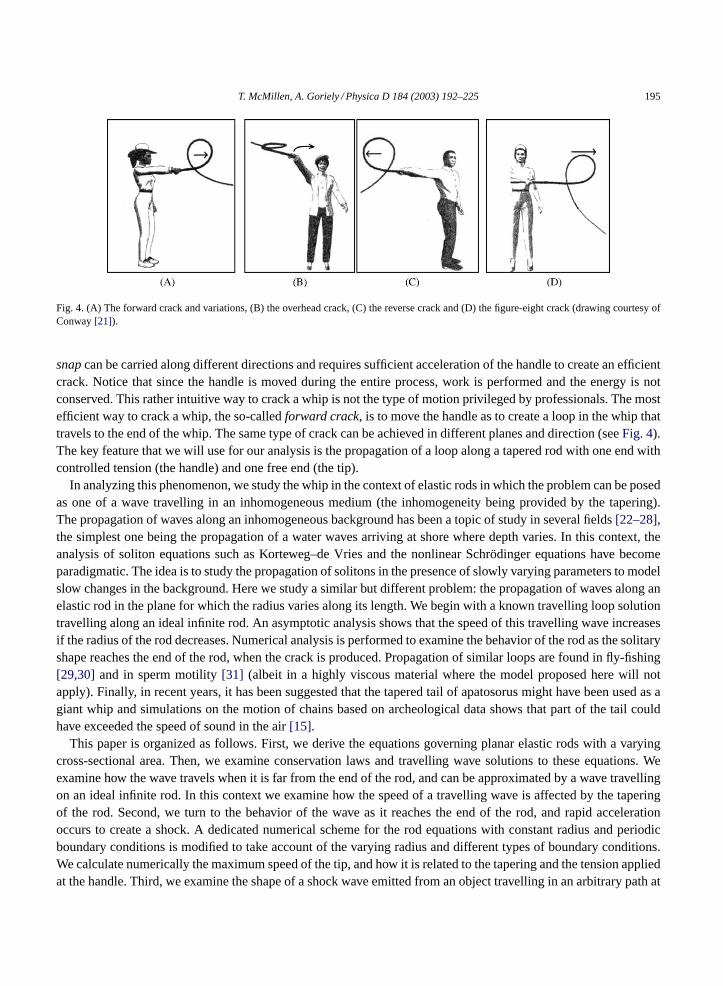
Fig. 4. (A) The forward crack and variations, (B) the overhead crack, (C) the reverse crack and (D) the figure-eight crack (drawing courtesy ofConway[21]).

snapcan be carried along different directions and requires sufficient acceleration of the handle to create an efficientcrack. Notice that since the handle is moved during the entire process, work is performed and the energy is notconserved. This rather intuitive way to crack a whip is not the type of motion privileged by professionals. The mostefficient way to crack a whip, the so-calledforward crack, is to move the handle as to create a loop in the whip thattravels to the end of the whip. The same type of crack can be achieved in different planes and direction (seeFig. 4).The key feature that we will use for our analysis is the propagation of a loop along a tapered rod with one end withcontrolled tension (the handle) and one free end (the tip).

In analyzing this phenomenon, we study the whip in the context of elastic rods in which the problem can be posedas one of a wave travelling in an inhomogeneous medium (the inhomogeneity being provided by the tapering).The propagation of waves along an inhomogeneous background has been a topic of study in several fields[22–28],the simplest one being the propagation of a water waves arriving at shore where depth varies. In this context, theanalysis of soliton equations such as Korteweg–de Vries and the nonlinear Schrödinger equations have becomeparadigmatic. The idea is to study the propagation of solitons in the presence of slowly varying parameters to modelslow changes in the background. Here we study a similar but different problem: the propagation of waves along anelastic rod in the plane for which the radius varies along its length. We begin with a known travelling loop solutiontravelling along an ideal infinite rod. An asymptotic analysis shows that the speed of this travelling wave increasesif the radius of the rod decreases. Numerical analysis is performed to examine the behavior of the rod as the solitaryshape reaches the end of the rod, when the crack is produced. Propagation of similar loops are found in fly-fishing[29,30] and in sperm motility[31] (albeit in a highly viscous material where the model proposed here will notapply). Finally, in recent years, it has been suggested that the tapered tail of apatosorus might have been used as agiant whip and simulations on the motion of chains based on archeological data shows that part of the tail couldhave exceeded the speed of sound in the air[15].

This paper is organized as follows. First, we derive the equations governing planar elastic rods with a varyingcross-sectional area. Then, we examine conservation laws and travelling wave solutions to these equations. Weexamine how the wave travels when it is far from the end of the rod, and can be approximated by a wave travellingon an ideal infinite rod. In this context we examine how the speed of a travelling wave is affected by the taperingof the rod. Second, we turn to the behavior of the wave as it reaches the end of the rod, and rapid accelerationoccurs to create a shock. A dedicated numerical scheme for the rod equations with constant radius and periodicboundary conditions is modified to take account of the varying radius and different types of boundary conditions.We calculate numerically the maximum speed of the tip, and how it is related to the tapering and the tension appliedat the handle. Third, we examine the shape of a shock wave emitted from an object travelling in an arbitrary path at


greater than the speed of sound, and apply this to determine the shock waves emitted from the tip of a whip as it iscracked.

2. Assumptions and governing equations

We model a whip as an elastic rod[32,33]. Most whips are made from leather, whose elastic constants are known[34]. However, whips can be made from such mundane items such as strings, cotton ropes, or even wet towels[35].In any case, the materials that various whips are made from can all be reasonably modeled as elastic rods. Themost efficient means of cracking a whip involve sending a planar loop (Fig. 4) down the whip, so we assume thatthe rod lies in the Euclideanx–y plane, and since the same crack can be performed in vertical or horizontal planeswe neglect the effect of gravity. We also assume that the rod: (i) has circular cross-sections with varying radiusR(s), (ii) is inextensible, (iii) is unshearable, (iv) obeys a linear constitutive relationship and, (v) the propertiesof the material, such as the density and elastic properties, are constant. We neglect in our analysis the effect ofair friction. This effect is crucial to understand the formation of a sonic boom but not for the acceleration of theloop itself.

Let (ex, ey, ez) be a fixed orthonormal basis in the Euclidean space and letr(s, t) = xex + yey ≡ (x(s, t), y(s, t))

be the centerline of the rod in thex–y plane, wheres is the arc-length andt is time. The tangent vectort isgiven by

t = ∂r∂s

= txex + tyey. (1)

We define the angleϕ (seeFig. 5) to be the angle betweenex andt so that

tx = cos(ϕ), (2)

ty = sin(ϕ). (3)

From Frenet’s equations[36], we have thatt′ = κn, wheren is the normal to the curver andκ is the curvature so thatκ = ϕ′. (Here(·)′ denotes differentiation with respect to the arc-lengths, and we will denote by˙(·) differentiationwith respect to timet.) We call the force and momentF = Fex + Gey andM, respectively. The balance of linearmomentum gives

ρAx = F ′, (4)

ρAy = G′, (5)

R0

t(s,t)

φ(s,t)r(s,t)

x

y

R(s)

Fig. 5. A rod in the plane. The centerline of the rod isr.


whereρ is the density per unit volume, andA = A(s) is the cross-section area at the material points. The linearconstitutive relationship, relating the moment to the strainκ, is, with M = Mez,

M = EIκ = EIϕ′, (6)

whereE is the Young’s modulus andI = I(s) the moment of inertia of the circular cross-section. The balance ofangular momentum generates an equation forϕ,

ρIϕ = (EIϕ′)′ +G cos(ϕ)− F sin(ϕ). (7)

Since the cross-sections are circular, we have

A = πR2, I = 14(πR

4), (8)

whereR = R(s) is the radius of the cross-section. We use the following scaling:

t = R0

2

√ρ

Et, s = R0

2s, (9)

r = 12(R0)r, F = EπR2

0F, (10)

whereR0 = R(0) is the radius of a cross-section at a given reference point. Notice that, in this scaling, whens = 1,s = R0/2, so the radius of the rod in the new variables is 2 at the reference cross-sectionR = R0. Furthermore,from (7), we see that the speed of sound in the rod is

cm =√E

ρ. (11)

To relate the speed of a wave in the new variables to the speed in the original variables we notice that a speed of 1in the new variables corresponds to�s/�t = 1, and that

�s

�t= cm

�s

�t, (12)

so that a speed of 1 in the scaled variables corresponds to the speed of sound in the material (note that the rodis modeled as being inextensible and therefore sound waves cannot travel in the material. Nevertheless, the valuecm still provides the proper scaling for flexural waves). The speed of sound in leather is approximately 220 m/s,comparable to the speed of sound in air, 330 m/s[34].

We define the ratio of the area of the cross-section to the reference cross-sectional area,

δ(s) = R2(s)

R20

. (13)

If the radius is constant,δ ≡ 1. Then, the equations become, after scaling and dropping the tildes,

δx = F ′, (14)

δy = G′, (15)

δ2ϕ = (δ2ϕ′)′ +G cosϕ − F sinϕ (16)

To obtain a closed system of equations for(F,G, φ), we divideEqs. (14) and (15)by δ, and differentiate with respectto s:

( cosϕ)·· =(F ′

δ

)′, (17)


( sinϕ)·· =(G′

δ

)′, (18)

δ2ϕ = (δ2ϕ′)′ +G cosϕ − F sinϕ. (19)

3. Boundary conditions and conservation laws

The evolution of an initial impulse depends heavily on the boundary conditions. In this section we explain thevarious boundary conditions and their physical significance, and derive several conservation laws for the differentcases.

The crack of the whip is created as the wave reaches the end of the whip and creates a rapid acceleration in thetip. The study of how this acceleration is produced will be done in two stages. First, we study the wave as it proceedsdown the rod, when it is far from the end. By considering the wave to be travelling on an infinite rod, we can deriverelations between the speed of the wave and the radius of the cross-section, and show that the speed of the waveincreases as the rod tapers. Then, we turn our attention to the behavior of the rod as the wave reaches the end of therod and the crack is produced. The study of the behavior of the wave as it reaches the end of the rod is performednumerically.

The first case we examine is a quasi-periodic, energy conserving case. In this case, the tension at the two endsof the rod is the same, and so does not represent the case of the whip, in which one end is free. However, byconsidering a loop travelling far from the end, and taking the ideal case in which the rod is infinite, we can makeseveral deductions analytically. This case is also used as a benchmark for our numerical method as it has beenstudied extensively for the case of constantδ (for example[37,38]) and we extend some of these results to the caseof a varying cross-sectional area.

For a real whip the end that cracks isfree, that is, no force or moment is imposed. The boundary condition at thisend is that the tension and curvature vanish. Thus, for the whip, the boundary condition at the free end is

ϕ′ = F = G = 0. (20)

We consider a whip of lengthL, wheres = 0 corresponds to the point where the rod meets the handle of the whipands = L corresponds to the free end. There are several realistic conditions for the left (handle) end. We considerthree cases, two in which the angle of the rod at the handle end is fixed, i.e.ϕ(s = 0) = 0, and one in which the rodat the handle end is allowed to swivel, i.e.ϕ′(s = 0) = 0. For the two cases in which the angle at the handle end isfixed, we consider one case in which a constant tension is applied at the handle end, and one in which the handleend is fixed. The latter case corresponds to the physical case of sending a loop down the rod, and then holding thehandle end so that it does not move. The case of constant tension at the left end has the obvious physical significanceof sending a loop down the rod and then pulling on the handle to give the tip a further kick. The four cases areconsidered as follows:

• Case I (quasi-periodic tension and angle):

ϕ(b, t) = ϕ(a, t)+ 2πk, δ2(a)ϕ′(a, t) = δ2(b)ϕ′(b, t), F(a, t) = F(b, t), G(a, t) = G(b, t),

δ(b)F ′(a, t) = δ(a) F ′(b, t), δ(b)G′(a, t) = δ(a)G′(b, t). (21)

• Case II (no tension at right end, constant tension at left end):

ϕ′(b, t) = 0, F(b, t) = G(b, t) = 0, ϕ(a, t) = 0, F(a, t) = α, G(a, t) = 0. (22)


• Case III (no tension at right end, left end fixed):

ϕ′(b, t) = 0, F(b, t) = G(b, t) = 0, ϕ(a, t) = 0, x(a, t) = y(a, t) = 0. (23)

• Case IV (no tension at right end, left end fixed, left end allowed to swivel):

ϕ′(b, t) = 0, F(b, t) = G(b, t) = 0, ϕ′(a, t) = 0, x(a, t) = y(a, t) = 0. (24)

Of particular importance for our analysis is the role of conserved quantities such as energy and angular momentum.Systems(17)–(19)have several conservation laws (see[39]) of the form

Tt = Xs. (25)

The first of these is related to the energy density

T = 12[δ2ϕ2

t + δ2ϕ2s + δ(x2

t + y2t )], (26)

X = δ2ϕsϕt + Fxt + Gyt . (27)

Thetotal energyH is

H(t) =∫ b

a

T ds = 1

2

∫ b

a

[δ2ϕ2s + δ2ϕ2

t + δ(x2 + y2)] ds, (28)

wherea andb are the endpoints of the rod, which may be infinite. The integrand ofH can be written as the sumof a potential and a kinetic energy,V + K, whereV = δ2ϕ2

s , andK = δ2ϕ2t + δ(x2 + y2). The potential energy

V = δ2κ2, which is the elastic energy of the rod. The first term ofK is δ2ϕ2 = δ2ω2, which is the kinetic energyassociated with a rotation of the basis vectors, or in other words, the rotational kinetic energy. The last term inK isδv2, the translational kinetic energy. From the conservation law(25), we see that

d

dtH = X(b, t)−X(a, t). (29)

Thus, the energy at any given time depends on the boundary conditions. In Case I,

dH

dt= F(b, t)

d

dt

∫ b

a

cosϕ ds +G(b, t)d

dt

∫ b

a

sinϕ ds. (30)

The boundary conditions(21) imply that

d2

dt2

∫ b

a

cosϕ ds = d2

dt2

∫ b

a

sinϕ ds = 0, (31)

so that if

d

dt

(∫ b

a

cosϕ ds

)∣∣∣∣∣t=0

= d

dt

(∫ b

a

sinϕ ds

)∣∣∣∣∣t=0

= 0, (32)

then energy is conserved,

dH

dt= 0. (33)

Eq. (32)is the compatibility conditions for conservation of energy in Case I, and we will assume that they holdthroughout the paper when we discuss this case. In Case II, work is performed, so energy is not conserved, and

H = −αx(a, t)+H(0). (34)

In Cases III and IV, energy is conserved for all initial conditions satisfying the boundary conditions.


Another conservation law of the form(25) is given by

T = δ2ϕt + δxyt − δyxt , (35)

X = δ2ϕs + Gx− Fy, (36)

related to theangular momentumL,

L(t) =∫ b

a

T =∫ b

a

δ2ϕt + δxyt − δyxt ds. (37)

Angular momentum is only conserved in Case IV. We summarize the change in energy and angular momentum inthe following table.

Case I :d

dtH = 0,

d

dtL = G(a)

∫ b

a

cosϕ + F(a)

∫ b

a

sinϕ,

Case II :d

dtH = −αx(a, t), d

dtL = −δ2(a)ϕs(a)+ αy(a),

Case III :d

dtH = 0,

d

dtL = −δ2(a)ϕs(a),

Case IV :d

dtH = 0,

d

dtL = 0.

(38)

Eqs. (14) and (15)are conservation laws themselves, associated with thelinear momentaMx andMy,

Mx =∫ b

a

δxt ds, (39)

My =∫ b

a

δyt ds. (40)

In Case I the linear momenta are conserved, but in Cases II–IV, they change in proportion to the tension at the leftend.

4. Travelling wave solutions

The most efficient way to crack a whip is to send a planar loop down the whip (Fig. 4). Thus, a natural startingpoint for examining whip waves is the study of travelling wave solutions. The governingequations (17)–(19)supporta travelling loop solution in the case of constantδ. If we consider a wave travelling far from the endpoints, it canbe approximated by a wave travelling along an ideal infinite rod[40,41]. We will examine this case in order todetermine how a wave is altered as the radius of the rod is decreased, but is still far away from the end of the rod.The boundary conditions consistent with the travelling loop solution are not consistent with the free end conditionfor the whip, so this analysis only provides us with some insights on how the speed changes when the loop is farfrom the end. We first consider the case whereδ is constant, and look for travelling wave solutions of(17)–(19).Settingξ = s − ct,

δc2( cosϕ)′′ = F ′′, (41)

δc2( sinϕ)′′ = G′′, (42)


δ2(c2 − 1)ϕ′′ = G cosϕ − F sinϕ, (43)

where(·)′ = d(·)/dξ. We consider an infinite rod which is horizontal at−∞, and where the tension at−∞ is α.This imposes the boundary conditions

lims→−∞ ϕ = lim

s→−∞ G = 0, lims→−∞ F = α. (44)

IntegratingEqs. (41) and (42)twice, and imposing the above boundary conditions, we find

F = δc2 cos(ϕ)+ α− δc2, (45)

G = δc2 sin(ϕ). (46)

Substituting these into(43), we obtain the equation

γ2ϕ′′ = sin(ϕ), (47)

where

γ2 = δ2(c2 − 1)

δc2 − α. (48)

Eq. (47)is the “pendulum equation”, with the well-known solution

ϕ = 4 tan−1[exp

(±ξ − ξ0

γ

)]. (49)

This solution corresponds to a loop travelling to the right with speedc. The± sign in the exponent determineswhether the loop is above or below thex-axis. We can find the space curveR by solvingx′ = cos(ϕ), y′ = sin(ϕ),which yields (taking the+ sign, seeFig. 6)

x(s, t) = s − 2γ tanh

(s − ct

γ

), (50)

y(s, t) = 2γ sech

(s − ct

γ

). (51)

We see that Case I boundary conditions(21), and initial conditions(32)are satisfied, so the energyH is conserved.In fact, the energy on this solution is

H = 4δ[2c4δ− α(1 + c2)]√(δc2 − α)(c2 − 1)

. (52)

x

y

c

2γ

Fig. 6. Travelling wave solution.


We solve(48) for α, and using this in the above, we have two equations forδ andc:

H = 4δδc2 + δ+ γ2c2

γ, (53)

α = δ−δc2 + δ+ γ2c2

γ2. (54)

Therefore, we have a two-parameter family of travelling wave solutions depending on(H, α), or alternatively, on(c, γ). We will see that(53) holds, to first order ifδ is a slowly varying function of the arc-lengths. Then, if theenergyH is constant, we will have a way to solve for the speedc of the travelling wave as a function ofδ, and henceof s, for a slowly varying radius of the cross-section.

We also note that the material point at the top of the loop travels at twice the speed of the loop itself. This is actuallytrue for any travelling loop with constant shape and speed, regardless of the shape, by the following reasonings: (i)In the frame of reference moving at speedc, the speed of the travelling loop, all material points are travelling at thesame speedc′. (ii) In the travelling frame of reference, the shape is constant, and the material points simply travelalong the curve traced out by the loop. Therefore all points must travel at the same speed. (iii) The two speedsc′

andc are equal. That is, in the travelling frame of reference, the speed of material points along the curve traced outby the loop is the same as the speed of the travelling loop. If we think of a point far to the right of the loop, thenthe loop is travelling toward this point with speedc in the fixed frame of reference. Therefore, in the moving frameof reference, this point is travelling toward the loop with speedc. So, when a material point reaches the top of theloop, it is travelling at speedc in the moving frame of reference travelling at speedc. When the point reaches thetop of the loop, its velocity is tangential to thex-axis, so that it is travelling in the same direction as the loop itself.Thus, the velocity of the material point at the top of the loop is 2c. This means that for a simple travelling wave,the maximal speed of a point on the rod is twice the speed of the travelling wave itself. Another way to look atthe problem is to consider a vertical bicycle wheel rolled in a straight line at constant velocityc. A point on top ofthe wheel has a horizontal velocityc relative to the center of the wheel and hence an absolute horizontal velocity2c. This kinematic analysis of travelling waves on rods suggests a simple explanation of the observation by Krehl,Engemann and Schwenkel that the whip cracks when its maximal tip speed reaches about twice the speed of sound.We see that the loop reaches the speed of sound when the tip reaches twice the speed of sound. It suggests that itis the loop itself, and not the tip, that creates the shock which is not surprising since the loop is ahead of the tipand is subject to most of the interaction with the flow. However, this simple explanation will not suffice, due to thefact that the travelling wave solution does not satisfy the boundary conditions for the free end of a whip. When thetravelling wave reaches the end of the whip it unfolds and the travelling loop shape is destroyed; a realistic analysisof the emission of the shock wave by a movable boundary accelerating in a supersonic flow is necessary to fullyunderstand the nature of the phenomenon. Nevertheless, without a free boundary condition the maximal speed of apoint on a rod with constant radius is twice the speed of the initial travelling loop.

5. Speed of travelling wave on a slowly varying background

Next we study how the travelling wave is affected by a change in the cross-sectional area. We start with thetravelling wave solution(50) and (51)at s = −∞, and let it travel in the positives direction. How does the loopchange asδ(s) changes? To conserve the energy, the speed may increase as the rod tapers or the speed could stayconstant and the loop increase or decrease in size as to increase the kinetic or elastic energy. We show that forrealistic initial conditions, the speed does increase and the loop size is essentially constant. We consider a rod whosecross-section is slowly varying, and expand the conservation lawTt = Xs in ε. We show that, to first order, the


energy of the loop is constant. Doing so, one can write the speed of the travelling wave as a function of the slowlyvarying cross-sectional area.

Consider a rod whose radiusδ = δ(εs) varies slowly as a function of the arc-length, that isε � 1. We define thelong space variableS, and the travelling wave variableξ, as follows[22,42]:

S = εs, (55)

ξ = 1

ε

∫ S

0ζ(s)ds − t. (56)

Then,

∂t → −∂ξ, (57)

∂s → ζ(S)∂ξ + ε∂S. (58)

The motivation behind this change of variables is that we would like to determine how the speed and shape of theloop change when the cross-sectional areaδ changes. For the travelling loop whenδ is constant,ζ = 1/c. We will seethat, to first order, the speed of the loop is given by 1/ζ(S), a function of the long space variable. The conservationlaw, in these variables, is

Tξ + ζ(S)Xξ + εXS = 0. (59)

ExpandingT , X andζ in ε, and collecting terms in(59), we have

O(ε0) : T0ξ + ζ0X0ξ = 0, (60)

O(ε1) : T1ξ + ζ1X0ξ + ζ0X1ξ +X0S = 0. (61)

Integrating theO(ε1) equation with respect toξ, and assuming thatT andX vanish atξ = ±∞, we obtain thecondition

∂

∂S

∫ ∞

∞X0 dξ = 0. (62)

From theO(ε0) equation, we see that

∂

∂S

1

ζ0

∫ ∞

∞T0 dξ = 0. (63)

Note that(63)holds for an arbitrary conservation lawTt = Xs with appropriate boundary conditions. Now we takeT andX to be as in(26) and (27), and expandϕ in ε, with ϕ0 the travelling wave solution(49)

ϕ0 = 4 tan−1[exp

(± ξ

γ

)]. (64)

If we let

H = 1

ζ0

∫ ∞

∞T0 dξ, (65)

then dH/dS = 0. A straightforward calculation shows that

H = 4γδ

ζ0

[δ(1 + ζ2

0)

γ2+ 1

ζ20

]+ O(ε). (66)

We see that the energy relation(53)holds, in the case whenδ is a function ofS, and thatH is constant, to orderε.


The speedc and height 2γ of the loop, are given, to first order by

c(S) = 1

ζ0(S), γ(S) = γ

ζ0(S). (67)

We conclude that the relations(53) and (54)hold, in the case whenδ is a function ofS, and thatH is constant, toorderε.

We can now useEq. (53)to calculate the first order relation of the speedc as a function ofδ. There are severalcases, depending on the behavior of the tension and the height of the loop,α andγ. We will see in the numericalexperiments below, with quasi-periodic boundary conditions on a finite interval, that the height of the loop remainsmostly constant, while the tension at the ends varies.

Solving(53) for c, the speed of the loop is given by

c2 = γH

4δ(δ+ γ2)− δ

δ+ γ2. (68)

This equation gives the speedc of the loop as a function ofδ, and hence ofs, to first order, in the case when theheight 2γ of the loop is constant, as in the quasi-periodic case. In the preceding equationH is determined by thespeed of the loop at any given point, such as the initial condition. Then the relation gives the speed at each pointalong the rod. We see that the speed decreases as the rod tapers, as expected, and thatc → ∞ as the rod tapers tozero,δ → 0. Notice also thatc as a function ofδ passes through zero atδ = √

γH/4 and that there is no (real)solution for largerδ. Thus, a wave that is travelling on a rod whose cross-sectional area isincreasingwill slowdown, and stop. At this reflection point all of the energy of the rod is potential. In the numerical experiments below,we show that the wave slows to zero speed, and then turns around and starts travelling in the opposite direction.

We may also consider the case of the infinite rod, in which the tension at the ends is held constant. In this caserelations(53) and (54)hold, to first order, withα constant. We can thus calculate both the speedc and height 2γ asfunctions of the radius of the rod. A straightforward calculation shows thatγ satisfies

f(γ) = γ4 − H4α

γ3 + δγ2 + Hδ4α

γ − 2δ3

α= 0. (69)

There are two cases, as illustrated inFig. 7:

Case 1 : c → ∞, γ → H

4αas δ → 0, (70)

Case 2 : c → 1, γ → 0 as δ → 0. (71)

Note that the curves(δ, γ) and(δ, c)must pass through(1, ·), sinceδ = 1 is the reference cross-section, which is whyin Fig. 7, only one branch of the curves represent the actual behavior ofc andγ. Let δ∗ be the point where two rootsof f(γ) become imaginary, andγl be the largest root off . We see that in the case wherec → 1, f ′(γl)|δ=δ∗ = 0,but in the case wherec → ∞, f ′(γl)|δ=δ∗ > 0. Thus, a bifurcation occurs whenf ′(γl)|δ=δ∗ goes to zero. Noticethat atδ = α,

f(γ) = (γ2 − α)(4αγ2 −Hγ + 8α2). (72)

Thus, atH2 − 128α3 = 0, two solutions coalesce. This is, in fact, the bifurcation point, because, at this point,γl = γ∗ = H/8α = √

2α−3/2,

f(γ∗)|H2=128α3 = f ′(γ∗)|H2=128α3 = 0, (73)

f ′′(γ∗)|H2=128α3 = 2α > 0, (74)


0.2 0.6 0.8 1 1.2δ

0.5

1

1.5

2

c,

0.6 0.8 1 1.2

0.5

1

1.5

2

c,

(a) (b)

(c) (d)

γ

γ

γ γ

f ( )γ δ=δ*

δ*δ*

δ

f ( )γ δ=δ*

Fig. 7. Two possibilities: either (a) c goes to ∞, or (b) c goes to 1 as δ → 0. The solid curve is c; the dash-dotted curve is γ . The thicker curvesare the curves representing the behavior of c and γ . The graphs (c) and (d) represent f(γ) in the cases (a) and (b), respectively, at δ = δ∗, whereδ∗ is the point where two roots of f(γ) become imaginary.

and the γ and c curves cross at

δ = α, γ =√

2α−3/2, δ = α, c = 1, (75)

respectively. The behavior of c as δ → 0 also depends on which branch of the curve c is on. Since γ and c must bedefined at δ = 1, the reference ratio of areas, we define the initial speed and height of the travelling wave to be atδ = 1:

ci = c(δ = 1), γi = γ(δ = 1). (76)

We note that if ci > 1 then c → ∞ as δ → 0. Therefore, we have the conditions

if H2 − 128α3 > 0 or ci > 1 then c → ∞, γ → 14 (H)α as δ → 0, (77)

if H2 − 128α3 < 0 and ci < 1 then c → 1, γ → 0 as δ → 0. (78)

Since the radius of the rod in the scaled variables is 2, it must be that γi > 2 to be physically realistic. We computethe behavior for realistic rods as follows. Note that

H2 − 128α3 = 16

γi6{γ4

i [1 + c2i (γ

2i + 1)]2 − 8[1 + c2

i (γ2i − 1)]3}. (79)


0.2 α 0.6 0.8 1

0.5

1

1.5

2δ

H

4 α

c(δ)

g(δ)

δ4 α

δ8 α

1/2

0.2 0.6 1 1.20.80.4

0.5

1

1.5

2

2.5

3

3.5

4

δ

c,γ

(a) (b)

Fig. 8. (a) The curves c and γ at the bifurcation point,H2 − 128α3 = 0. (b) If ci > 1 then c → ∞ as δ → 0.

Thus, for 0 ≤ ci ≤ 1, γi ≥ 1,

H2 − 128α3 ≥ 16

γ6i

{γ4i [1 + c2

i (γ2i − 1)]2 − 8[1 + c2

i (γ2i − 1)]3}

= 16

γ6i

[1 + c2i (γ

2i − 1)]2{γ4

i − 8[1 + c2i (γ

2i − 1)]} > 0 (80)

if γi > 23/4. Since we assume that the initial speed of a loop is subsonic, and the radius of the rod is 2, all physicallyrealistic solutions have 0 ≤ ci ≤ 1, γi ≥ 23/4. Thus, for all physically realistic cases c → ∞ as δ → 0.

We further note that, as in the case of constant loop size, in the case when the tension is held constant, a looptravelling on a rod whose cross-sectional area is increasingwill slow down, and stop. The point at which the wavestops is determined by finding the value of δ = H/4

√α such that c = 0 (see Figs. 7 and 8).

6. Numerical simulations

We now turn to a complete description of the behavior of the whip with realistic boundary conditions. The analysispresented above can only be applied away from the end when the assumptions on the variation of tension and theboundary conditions are valid. Close to the end, a numerical analysis is necessary to complete the description. Adedicated scheme for solving (17)–(19) was developed by Falk and Xu [38,43,44]. This scheme was developedfor the particular case (Case I) of a constant radius and periodic boundary conditions. We present an extension ofthe scheme to incorporate the varying radius and different boundary conditions. While the inclusion of tapering inthe algorithm is straightforward the main challenge is to adapt it as to include different types of realistic boundaryconditions and prove the conservation of discrete versions of the conservation laws (such as energy and angularmomentum).

We discretize the interval [0, L] into N equally spaced mesh points sj , sj+1 − sj = L/N = h, and time isdiscretized into steps of duration τ, with the ratio ν = τ/h set equal to 1/2, below the limit of the classical CFL


condition for stability, ν = 1/√

2 (cf. [45, p. 489]). The discrete version of (17)–(19) is

�2τ cos θnj = �+

h

{1

δj�−h f

nj

}, (81)

�2τ sin θnj = �+

h

{1

δj�−h g

nj

}, (82)

�2τθ

nj −�2

hθnj = 1

δ2j

�+h δ

2j�

+h θ

nj + 1

δ2j

[gnjCn(θj)− fnj S

n(θj)], (83)

where

Sn(θj) =

−( cos θn+1j − cos θn−1

j )

θn+1j − θn−1

j

if θn+1j �= θn−1

j ,

sin θn−1j if θn+1

j = θn−1j ,

(84)

Cn(θj) =

sin θn+1j − sin θn−1

j

θn+1j − θn−1

j

if θn+1j �= θn−1

j ,

cos θn−1j if θn+1

j = θn−1j ,

(85)

δj = δ(hj), and θnj , fnj , and gnj are approximate values of ϕ(jh, nτ), F(jh, nτ), andG(jh, nτ). The discrete derivatives

are defined by

�2τu

nj = 1

τ2(un+1

j − 2unj + un−1j ), �2

hunj = 1

h2(unj+1 − 2unj + unj−1), (86)

�−h u

nj = 1

h(unj − unj−1), �+

h unj = 1

h(unj+1 − unj ). (87)

The discrete versions of x and y are,

xnj = xna + h

j−1∑i=1

cos θni , (88)

ynj = yna + h

j−1∑i=1

sin θni , (89)

where xna and yna will be determined from the conditions

�2τx

nj = 1

δj�−h f

nj , (90)

�2τy

nj = 1

δj�−h g

nj . (91)

It is clear from the definition that

�+h x

nj = cos θnj , (92)

�+h y

nj = sin θnj . (93)


The discrete boundary conditions, corresponding to the four cases (21)–(24), are:

• Case I (quasi-periodic tension and angle):

fn0 = fnN, gn0 = gnN, θn0 + 2πk = θnN, δ20(θ

n1 − θn0 ) = δ2

N(θnN+1 − θnN),

δ1(fnN+1 − fnN) = δN+1(f

n1 − fn0 ), δ1(g

nN+1 − gnN) = δN+1(g

n1 − gn0). (94)

• Case II (no tension at right end, constant tension at left end):

fn0 = α, gn0 = 0, gnN = fnN = 0, θnN+1 = θnN, θn0 = 0. (95)

• Case III (no tension at right end, left end fixed):

fnN = gnN = 0, θnN+1 = θnN, θn0 = 0, xna = yna = 0. (96)

• Case IV (no tension at right end, left end fixed, left end allowed to swivel):

fnN = gnN = 0, θnN+1 = θnN, θn0 = θn1 , xna = yna = 0. (97)

The main idea behind the scheme is to solve (81) and (82) for fnj , gnj , and use these values to form one semilinear

equation for θnj from (83), which is solved for θn+1j , iteratively. The method is designed to preserve a discrete version

of the energy. The discrete energy is given by

En = h

2

N∑j=1

{δ2j (�

+τ θ

nj )

2 + δ2j (�

−h θ

nj )(�

−h θ

n+1j )+ δj[(�

+τ x

nj )

2 + (�+τ y

nj )

2]}. (98)

Conservation of energy is central to the development of the method, so we first present the following lemma (for aproof see Appendix A).

Lemma 6.1. For everyn ≥ 0, we haveEn+1 = En + Rn, whereRn is given by

Rn = 12 [δ2

N+1�+h θ

nN(θ

n+1N − θn−1

N )− δ21�

+h θ

n0 (θ

n+10 − θn−1

0 )+ fnN(xn+1N+1 − xn−1

N+1)

− fn0 (xn+11 − xn−1

1 )+ gnN(yn+1N+1 − yn−1

N+1)− gn0(yn+11 − yn−1

1 )]. (99)

We see how the energy is conserved in the four cases. In Case I, the equations and boundary conditions imply that

�2τ

N∑j=1

cos θnj = 0. (100)

Thus, if

N∑j=1

cos θ0j =

N∑j=1

cos θ1j , (101)

N∑j=1

sin θ0j =

N∑j=1

sin θ1j , (102)

then Rn = 0, and the discrete energy is conserved in Case I. In [43], Coleman and Xu present an algorithm forcalculating θ0,1

j such that (101) and (102) hold.


In Case II, we have

Rn = − 12 (α)(x

n+11 − xn−1

1 ). (103)

In Cases III and IV, Rn = 0, and the discrete energy is conserved. We also define the discrete angular momentum

Ln = h

N∑j=1

{δ2j�

+τ θ

nj + δj(x

nj�

+τ x

n−1j − ynj�

+τ y

n−1j )}. (104)

The discrete angular momentum is not conserved in any of the four cases. This is due to the fact that we use anapproximation for the cosine and sine in (83), but fluctuations in the discrete angular momentum in Case IV arevery small, and decrease to zero as the number of spatial points is increased. Details on the numerical scheme andits implementation are provided in Appendix A.

6.1. Numerical results

As a benchmark, we first compare the results in the quasi-periodic case, starting with the known travelling wavesolution, to see that the analytic solution is recovered. We also verify that the energy is conserved, and matchesthe analytically determined energy. Fluctuations in the energy occur because of the necessity of accepting anapproximate solution to the semi-linear equation (A.30) for θnj , and in Case I additional fluctuations occur due to thefact that

∑cos θnj is not conserved exactly. In Case I, fluctuations in the energy were always less than 0.008%, and

in Cases III and IV always less than 0.00005%. In Case IV, where the analytical angular momentum is conserved,the fluctuations in the discrete angular momentum were always less than 0.0007%.

Case I. Results of numerical calculations for constant δ are summarized by Coleman and Xu [43]. When weallow the radius of the rod to vary, we obtain results consistent with the analytical predictions, i.e. that the speedincreases or decreases as the cross-sectional area decreases or increases, according to relation (68) the speed of theloop is given by

c2 = γH

4δ(δ+ γ2)− δ

δ+ γ2. (105)

Calculations in Case I are done in the scaled variables. Figs. 9 and 10 show results in the case where the radius isdecreasing, and Figs. 9 and 10 show results in the case where the radius is increasing. From Figs. 9 and 11 we seethat the height of the loop remains almost constant as the speed increases and decreases, respectively. This is, in fact,generally true. Thus, we may calculate the speed of the travelling loop from (105) and compare it with the speedcalculated numerically. In Figs. 10B and 12B we see that the analytically and numerically computed speeds matchalmost identically. In Figs. 10 and 12 are two graphs. In graph (A) we show the speed of the loop as a function oftime. On the same graph is shown the value of δ at the material point at the top of the loop. In graph (B) the speed of

0 2

1

4 6 8 10 12 14 16 18 20

x

yTraveling wave

Accelerated wave1

t=0 2.5 5 7.5 10

t=0 2.5 5 7.5 10

Fig. 9. Traveling wave solution with δ = 1 (top) and numerical solution at times t = 0, 2.5, 5, 7.5, 10 with δ(s) = 1 − (1/2)(s/L).


0.7 0.75 0.8 0.85 0.90.5

0.55

0.6

0.65

0.7

0.75

0.8

0.85

0.9

δ

loop speed

xx

xx

xx

x xx

xx

x xxx

x xxxx

xxxx

x

x

Fig. 10. Speed of loop as a function of δ with λ = 1/2. The solid curve is the analytically computed speed of the loop, as determined from (105),and the +’s are the numerically computed speed of the loop.

the loop is shown as a function of δ, by computing the speed of the loop at each time step, and plotting that againstthe value of δ at the material point at the top of the loop. In Figs. 11 and 12 are shown the results of calculations fora rod whose radius is increasing. We see that the speed of the loop decreases to zero, and then the loop turns aroundand travels in the opposite direction.

Case II. In order to measure the effects of the boundary conditions, tension and tapering in the rod on the maximalspeed of the tip of the rod, we must take into account how the material points behave without these effects. Sincethe speed of the material point at the top of a travelling loop is twice the speed of the loop itself, we define a newquantity to measure the increase of the maximum speed of a material point on the rod:

σ = maximum speed of tip

2ci, (106)

where ci is the initial speed of the loop. We see that without the free boundary condition, and without tapering, forthe travelling loop, σ = 1. Thus, σ measures the increase in the maximal speed of the tip due to the various effectswe consider. For the simulations in which we compare the tapering and the tension to the maximum speed of thetip, we take the initial loop to be centered on the rod, that is, the top of the loop is at s = L/2. The tapering of therod is chosen to be a linear function,

δ(s) = 1 − λs

L. (107)


0 2 4 6 8 101

0

1

2

0 2 4 6 8 101

0

1

2

0 2 4 6 8 101

0

1

2

0 2 4 6 8 101

0

1

2

0 2 4 6 8 101

0

1

2

0 2 4 6 8 101

0

1

2

0 2 4 6 8 101

0

1

2

0 2 4 6 8 101

0

1

2

0 2 4 6 8 101

0

1

2

0 2 4 6 8 101

0

1

2

Fig. 11. Traveling wave for δ = 1 (left) and numerical solution at times t = 0, 3.75, 7.5, 11.25, 15 with δ(s) = (1/2)(1 + (s/L)).

0.62 0.64 0.66 0.68 0.7 0.72 0.740.6

0.4

0.2

0

0.2

0.4

0.6

δ

loop speed

Analytical

Numerical

0 2 4 6 8 10 12 14 16 180.6

0.4

0.2

0

0.2

0.4

0.6

0.8

time

δloop speed

(A) (B)

Fig. 12. (A) Speed of loop and δ at the top of the loop as a function of time, for an increasing radius, δ(s) = (1/2)(1 + (s/L)). (B) Speed ofloop as a function of δ. The analytical curve is computed from (105).


0 1 2 3 4 5 6 7 80

5

10

15

20

25

30

35

tension (kN)

c =0.1, =0c =0.2c =0.5c =0.1, =0.9c =0.2c =0.5

λ

λ

i

ii

ii

iσ

Fig. 13. Maximum tip speed vs. tension at handle in Case II. In this case, the rod is 2 m long, and the typical radius is 1 cm. The height of theinitial loop 2γi is γi = L/10.

Thus, λ is a measure of the tapering in the rod. A rod without tapering has λ = 0, and a rod that tapers to zero radiusat its tip has λ = 1.

When we apply a fixed tension at the handle end, energy is not conserved, as work is performed when the leftend accelerates. In Fig. 13 we see that the maximum tip speed increases (almost) linearly as the tension appliedat the left end increases. No general relation between σ and the tension applied at the handle is computed, as themaximal tip speed depends also on the initial speed and size of the loop. However, we see that for a given initialspeed and size of the loop, the maximal tip speed is almost linear in the applied tension. We also note that theacceleration of the tip is greater when the initial speed of the loop is smaller, although the final tip speed is greaterfor a faster initial speed. In Fig. 14 we see the result of one simulation in Case II, as the whip unfolds. In this case,the loop is started toward the right end of the rod, and a large tension is applied at the left end. If one applies thesame tension with a loop at the middle of the rod, the loop is simply pulled through, and the acceleration of thetip is not great. Such a case is seen in Fig. 15. The lesson is that in order to produce a large acceleration in the tip,the loop must accelerate until it is close to the end of the rod. This is consistent with the way whips are cracked:one sends a loop down the rod, which accelerates as the rod tapers, and then one applies a tension as the loopreaches the end of the rod to provide an extra kick. In this way, a large acceleration, with an associated loud crack, isproduced.

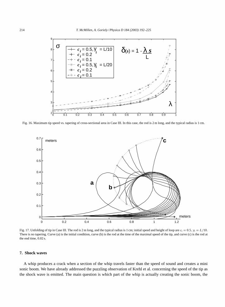
Case III. In Fig. 16 we see the results of several simulations, in which the maximum speed of the tip is comparedwith the tapering in the rod. We show several simulations with different values of the tapering λ. We see that for anuntapered rod, for which λ = 0, the maximum speed of the tip is between 4 and 6 times the initial speed of the loop,


0 0.5 1 1.5 2 2.5

-0.4

-0.2

0

0.2

meters

meters

Fig. 14. Unfolding of tip in Case II. The rod is 2 m long, and the typical radius is 1 cm; initial speed and height of loop are ci = 0.5, γi = L/10;applied tension is 120 kN. Elapsed time is 0.007 s.

or σ is between 2 and 3, the acceleration due solely to the free boundary condition. This acceleration, sometimesrefer to as the “Kucharski effect” is due to the rotation of the tip around the horizontal axis as the loop reaches theend [16]. As the tapering increases the maximum speed of the tip increases. At the maximal tapering, when the areaof the cross-section at the end of the tip is 1/20 the area at the handle, we get another doubling of the maximum tipspeed. Again, no general relation between the tapering and the maximal tip speed has been found analytically, buta general trend can be observed. The maximal tip speed increases nonlinearly as a function of the tapering, with noobvious scaling. We do see, however, that the tapering has a greater effect on the maximal tip speed than does theincrease of applied tension in Case II. As in Case II, acceleration is greater for a slower initial speed, although fora greater initial speed, the maximal tip speed is greater. Fig. 17 shows a result of one simulation in this case, as thetip of the whip unfolds.

Case IV. Results in Case IV, where the whip is allowed to swivel at the handle, are essentially indistinguishablefrom Case III. That is, there seems to be no advantage or disadvantage in allowing the swiveling, at least in the casewhere a loop is sent down the whip as we have prescribed. This could explain why there seems to be no preferenceamong whip-makers for swiveling or non-swiveling thongs.

0.2 0.4 0.6 0.8 1 1.2 1.4 1.6 1.8

0.2

0

0.2

meters

meters

b.a.

c.d.

e.

Fig. 15. High tension applied too early in Case II. The rod is 2 m long, and the typical radius is 1 cm; initial speed and height of loop areci = 0.1, γi = L/10; applied tension is 80 kN. The triangles are the left (handle) end of the whip, and the thicker curve is the initial condition.Elapsed time is 0.005 s.


0 0.1 0.2 0.3 0.4 0.5 0.6 0.7 0.8 0.9 12

3

4

5

6

7

8

9

λ

δ(s) = 1 - λ sc = 0.5, = L/10c = 0.2c = 0.1c = 0.5, = L/20c = 0.2c = 0.1

γ

γi i

i

iiiii

σ

L

Fig. 16. Maximum tip speed vs. tapering of cross-sectional area in Case III. In this case, the rod is 2 m long, and the typical radius is 1 cm.

0 0.2 0.4 0.6 0.8 1 1.2

0

0.1

0.2

0.3

0.4

0.5

0.6

0.7

meters

meters

ab

c

Fig. 17. Unfolding of tip in Case III. The rod is 2 m long, and the typical radius is 1 cm; initial speed and height of loop are ci = 0.5, γi = L/10.There is no tapering. Curve (a) is the initial condition, curve (b) is the rod at the time of the maximal speed of the tip, and curve (c) is the rod atthe end time, 0.02 s.

7. Shock waves

A whip produces a crack when a section of the whip travels faster than the speed of sound and creates a minisonic boom. We have already addressed the puzzling observation of Krehl et al. concerning the speed of the tip asthe shock wave is emitted. The main question is which part of the whip is actually creating the sonic boom, the


Fig. 18. The Mach cone of an object travelling in a straight line. (b) A bullet travelling faster than the speed of sound. (b) Illustration of the Machcone. The thinner circles are the sound waves, the thicker lines are the shock waves. The dashed line is the path of the object.

tip or a section of the whip. To try to answer this question, we compute the geometric (linear) shock wave that isemitted by the tip as the whip unfolds.

When an object travels faster than the speed of sound, a shock waveis formed. For an object travelling in a straightline, the first approximation of the shock wave is given by the Mach cone, because the shock wave is in the shapeof a cone following the object. This phenomenon can be observed, for example, in the wake that follows a swiftlymoving boat, or in the shock wave following a bullet, as in Fig. 18a. We now compute a similar approximation forthe shape of the shock wave in the case of an object travelling in an arbitrary path. We will apply this to the case ofthe tip of the cracking whip to see how the shock wave emanates from a cracking whip.

In the linear theory, a shock wave is formed by the envelope of infinitely many sound wave fronts meeting at thesame curve. Consider first the case of an object travelling with constant speed along a straight line, as in Fig. 18.Let the speed of sound be vs, and the speed of the object be v0. If the object leaves the origin at time 0, it reaches(v0t, 0) at time t. Thus, let x(s) = (v0s, 0) be the path of the object. At each point s the object emits a sound wave,whose front at time t is a circle centered at (v0s, 0), with radius vs(t − s). The shock wave is the envelope of thesesound waves. At time t this is a curve which we call z(s; t).

We calculate the shock wave curve z(s; t) as follows. Let y(s; t) be the line from (v0s, 0) to the tangent of thecircle to x(t) = (v0t, 0). The Mach cone z is then determined as the set of all the tangent points. The angle betweeny(s; t) and x(s; t) is determined by the condition

cosβ = |y(s; t)|v0(t − s)

= vs(t − s)

v0(t − s)= vs

v0. (108)

Thus, the envelope z(s; t) is given by

z(s; t) = (v0s, 0)+ y(s; t), (109)

where y(s; t) is determined by the system

(1, 0) · y(s; t)|y(s; t)| = vs

v0, (110)

|y(s; t)| = vs(t − s). (111)

The envelope z(s; t) is a space curve defined for every t > 0, for 0 ≤ s ≤ t. In this case of an object travelling on astraight path with constant velocity, as in Fig. 18, the Mach cone at each time t, is given by

z(s; t) =(s + 1

v20

(t − s),±(t − s)

√1

v20 − 1

). (112)


β x’(s)∗ (t-s)

x(t)

x(s)

y(s;t)

z(s;t)

x(s) +

Fig. 19. The shock wave of an object travelling in a curved path. The thinner circles are the sound waves, the thicker lines are the shock waves.The dashed line is the path of the object.

The case of an object travelling on a straight path can be easily generalized to the case of an object travelling alongan arbitrary path, x(s). Again, the envelope of the sound waves, which is the shock wave, is given by the curvez(s; t). Apparently (see Fig. 19), z is given by

z(s; t) = x(s)+ y(s; t), (113)

where y(s; t) is determined by the system

x′(s)|x′(s)| · y(s; t)

|y(s; t)| = vs

v0, (114)

|y(s; t)| = vs(t − s). (115)

We can further generalize the above to the case of an object travelling along an arbitrary path with an arbitraryspeed. In the above, we have assumed that the speed of the object v0 is constant, or in other words that |x′(s)| ≡v0 = constant. Now we allow that v(s) = x′(s) varies along the path of the object. The distance the object travelsfrom s to t is

d(s; t) =∫ t

s

|v(s′)| ds′. (116)

Then, the shock wave is still given by (113), but with y defined by

x′(s)|x′(s)| · y(s; t)

|y(s; t)| = vs(t − s)∫ ts|v(s′)| ds′

, (117)

|y(s; t)| = vs(t − s). (118)

We note, also, that the above formulation is valid in three dimensions as well. Given a path x(s), in three-space, theshock wave is defined by (113), where y is defined by (117) and (118). The difference now is that these equationsdefine a curve, instead of two points, for each s, t. The shock wave, for each time t, is then a surface in three-space.For example, an object travelling at constant speed v0 along the x-axis would have the Mach cone,

z(s, θ; t) =(s + 1

v20

(t − s), cos (θ)(t − s)

√1

v20 − 1

, sin (θ)(t − s)

√1

v20 − 1

), (119)

a surface for each time t.

7.1. Numerical computation of shock waves

We now compute the shock wave which is the crack of the whip, for the simulation seen in Fig. 14. In Fig. 20 wesee the results of this calculation, in which shock waves are computed coming from the tip of the rod. Comparing


0.5 1 1.5 2 2.5 3

1

0.5

0

0.5

1

meters

meters

Fig. 20. Numerical solution in Case II at various times. The solid curves are the rod; the dashed curve is the path the tip of the whip travels; thedash-dotted curves are the shock waves.

this result to the photographs of Krehl et al. in Fig. 1, we see that the shock waves as computed from coming off ofthe curve the tip of the whip travels, are consistent with those photographed in actual whip cracks. This suggeststhat is, in fact, the tip of the whip, or a small section of the rod near the tip, that produces the crack.

8. Conclusions

As anybody who has cracked a whip can attest, producing a loud crack requires a subtle combination of motionto create an initial loop and let it travel along the whip to the end. Similarly, we found at the numerical level, thatit takes a fair amount of experimenting with various boundary conditions, speeds and tensions, to find the correctparameters so that the tip accelerates sufficiently to produce a crack. The most efficient way to crack a whip, interms of producing the loudest crack for the least amount of effort, is to send a planar loop down a tapering rod withextra applied tension to provide further acceleration. The same type of motion is found in fly-fishing where tensionis used to optimize a throw [29].

The crack itself is a sonic boom created when a section of the whip at its tip travels faster than the speed of sound.The rapid acceleration of the tip of the whip is created when a wave travels to the end of the rod, and the energyconsisting of the kinetic energy of the moving loop, the elastic energy stored in the loop, and the angular momentum ofthe rod is concentrated into a small section of the rod, which is then transferred into acceleration of the end of the rod.

Several factors combine to create a wave with a high speed as it travels to the end of the rod. Additional tension atthe handle end, increasing the speed of the initial loop, and the tapering in the rod all serve to increase the maximumspeed of the tip of the rod. The main effect seems to be the tapering in the rod, which increases the maximal speed


nonlinearly. Thus, the main key in successful whip cracking seems to be in the design of an efficient elastic taperedwhip as both whip artists and craftspeople will tell you.

Acknowledgements

We thank Ph. Hanset, A. Ruina, and M. Tabor for discussions, and are indebted to A. Conway and P. Krehl forsharing their images of whips. TM is supported through the NSF-VIGRE initiative. AG is supported by the Sloanfoundation and the NSF grant DMS9972063.

Appendix A. Numerical scheme

A.1. Proof of Lemma 6.1

Lemma A.1. For everyn ≥ 0, we haveEn+1 = En + Rn, whereEn is defined by(98), andRn is given by

Rn = 12 [δ2

N+1�+h θ

nN(θ

n+1N − θn−1

N )− δ21�

+h θ

n0 (θ

n+10 − θn−1

0 )+ fnN(xn+1N+1 − xn−1

N+1)− fn0 (xn+11 − xn−1

1 )

+ gnN(yn+1N+1 − yn−1

N+1)− gn0(yn+11 − yn−1

1 )]. (A.1)

Proof. We first multiply Eq. (83) by δ2jh(θ

n+1j −θn−1

j ), and sum from j = 1 toN. The left-hand side of the resultingequation is, after summing by parts the second term, and simplifying,

LHS = h

N∑j=1

δ2j (�

+τ θ

nj )

2 − h

N∑j=1

δ2j (�

+τ θ

n−1j )2 + h

N∑j=1

δ2j�

−h θ

n+1j �−

h θnj − h

N∑j=1

δ2j�

−h θ

nj�

−h θ

n−1j

+h

N∑j=1

�−h δ

2j�

−h θ

nj (θ

n+1j−1 − θn−1

j−1 )− δ2N�

+h θ

nN(θ

n+1N − θn−1

N )+ δ20�

+h θ

n0 (θ

n+10 − θn−1

0 ). (A.2)

For the right-hand side of the equation we use the fact

cos θn+1j − cos θn−1

j =xn+1j+1 − xn−1

j+1 − xn+1j + xn−1

j

h, (A.3)

and hence

h

N∑j=1

fnj ( cos θn+1j − cos θn−1

j ) =N∑j=1

fnj (xn+1j+1 − xn−1

j+1 − xn+1j + xn−1

j )

= −N∑j=1

(f nj − fnj−1)(xn+1j − xn−1

j )+ fnN(xn+1N+1 − xn−1

N+1)− fn0 (xn+11 − xn−1

1 )

= −hN∑j=1

δj�2τx

nj (x

n+1j − xn−1

j )+ fnN(xn+1N+1 − xn−1

N+1)− fn0 (xn+11 − xn−1

1 ), (A.4)

and the fact that �2τx

nj (x

n+1j − xn−1

j ) = (�+τ x

nj )

2 − (�+τ x

n−1j )2, to compute


RHS = h

N∑j=1

�−h δ

2j�

−h θ

nj (θ

n+1j−1 − θn−1

j−1 )− h

N∑j=1

δj[(�+τ x

nj )

2 − (�+τ x

n−1j )2]

−h

N∑j=1

δj[(�+τ y

nj )

2 − (�+τ y

n−1j )2] + h(δ2

N+1 − δ2N)�

−h θ

nN+1(θ

n+1N − θn−1

N )

−h(δ21 − δ2

0)�−h θ

n1 (θ

n+10 − θn−1

0 )+ fnN(xn+1N+1 − xn−1

N+1)− fn0 (xn+11 − xn−1

1 )

+ gnN(yn+1N+1 − yn−1

N+1)− gn0(yn+11 − yn−1

1 ). (A.5)

Comparing the RHS with the LHS, we see that the lemma holds. �

A.2. Case I numerics

We first describe the numerical scheme for Case I. Then we will describe how the scheme is modified for CasesII and III.

We start by solving (81) and (82) for fnj , gnj . Setting

A1,1 = − 1

h2

(1

δ1+ 1

δ2

), A1,2 = 1

h2δ2, (A.6)

Aj,j−1 = 1

h2δj, Aj,j = − 1

h2

(1

δj+ 1

δj+1

), Aj,j+1 = 1

h2δj+1if 1 < j < N, (A.7)

AN,1 = 1

h2δ1, AN,N−1 = 1

h2δN, (A.8)

AjN = 1 for 1 ≤ j ≤ N, (A.9)

Aij = 0 otherwise, (A.10)

d = 1

h2

(1

δ0, 0, 0, . . . , 0,

1

δN,−

(1

δ1+ 1

δN

))T

, (A.11)

and

A+ij = (A−1)ij if i < N, A+

Nj = 0, (A.12)

bi = −(A−1d)i if i < N, bN = 1, (A.13)

and letting fnh = (f n1 , fn2 , . . . , f

nN)

T, and similarly for gnh, then (81) and (82) are solved by

fnh = bf n + A+(�2τ cos θn1 ,�

2τ cos θn2 , . . . , �

2τ cos θnN)

T, (A.14)

gnh = bgn + A+(�2τ sin θn1 ,�

2τ sin θn2 , . . . , �

2τ sin θnN)

T, (A.15)

where

f n = fn0 = fnN, gn = gn0 = gnN (A.16)

with the compatibility condition

�2τ

N∑j=1

cos θnj = 0, �2τ

N∑j=1

sin θnj = 0. (A.17)


In order to simplify notation, and conform to the notation in [43], we will call

c = (�2τ cos θn1 ,�

2τ cos θn2 , . . . , �

2τ cos θnN)

T,

s = (�2τ sin θn1 ,�

2τ sin θn2 , . . . , �

2τ sin θnN)

T, K = − 1

h(A+)T. (A.18)

We next make a few definitions to be used in the scheme.

Sn(θj) = 2∫ L

0

∫ L

0ξ sin (ηξθn+1

j + (1 − η)ξθnj + (1 − ξ)θn−1j ) dη dξ,

Cn(θj) = 2∫ L

0

∫ L

0ξ cos (ηξθn+1

j + (1 − η)ξθnj + (1 − ξ)θn−1j ) dη dξ,

Sn(θi, θj) = −Sn(θj)Cn(θi)+ Cn(θj)Sn(θi), Cn(θi, θj) = Sn(θj)S

n(θi)+ Cn(θj)Cn(θi). (A.19)

Next, we use the solution for f, g, to form a single semi-linear equation for θ. Substituting (A.14) and (A.15) into(83), we have

�2τθ

nj −�2

hθnj = 1

δ2j

�+h δ

2j�

+h θ

nj + bj

δ2j

[−f nSn(θj)+ gnCn(θj)] + 1

δ2j

[−(A+c)jSn(θj)+ (A+s)jCn(θj)].

(A.20)

A simple calculation shows that

cj = �2τ cos θnj = −Sn(θj)�2

τθnj − Cn(θj)�

+τ θ

nj�

+τ θ

n−1j , (A.21)

sj = �2τ sin θnj = Cn(θj)�

2τθ

nj − Sn(θj)�

+τ θ

nj�

+τ θ

n−1j . (A.22)

Another calculation shows

1

δ2j

[−(A+c)jSn(θnj )+ (A+s)jCn(θnj )] = h

δ2j

[−

N∑i=1

Kij Cn(θi, θj)�

2τθ

ni +

N∑i=1

Kij Sn(θi, θj)�

+τ θ

ni �

+τ θ

n−1i

].

(A.23)

Substitution into (A.20) yields

�2τθ

nj −�2

hθnj + h

δ2j

N∑i=1

Kij Cn(θi, θj)(�

2τθ

ni −�2

hθni ) = Bn(θh)j + bj

δ2j

[−f nSn(θj)+ gnCn(θj)], (A.24)

where

Bn(θh)j = 1

δ2j

�+h δ

2j�

+h θ

nj + h

δ2j

N∑i=1

Kij Sn(θi, θj)�

+τ θ

ni �

+τ θ

n−1i − h

δ2j

N∑i=1

Kij Cn(θi, θj)�

2hθ

ni . (A.25)


Summation by parts shows that

h

N∑i=1

Kij Cn(θi, θj)�

2hθ

ni = −

N∑i=2

(Kij Cn(θi, θj)−Ki−1,jC

n(θi−1, θj))�−h θ

ni

+ 1

h

(δ2

0

δ2N

KNjCn(θN, θj)−K1jC

n(θ1, θj)

)(θn1 − θnN + 2πk). (A.26)

Therefore,

Bn(θh)j = 1

δ2j

�+h δ

2j�

+h θ

nj + h

δ2j

N∑i=1

Kij Sn(θi, θj)�

+τ θ

ni �

+τ θ

n−1i

+ 1

δ2j

N∑i=2



ni

− 1

hδ2j

(δ2

0

δ2N

KNjCn(θN, θj)−K1jC

n(θ1, θj)

)(θn1 − θnN + 2πk). (A.27)

We are thus able to form the semi-linear equation. Setting

(Lθh)ij = h

δ2j

Kji Cn(θj, θi), (A.28)

An(θh)j = bjδ2j

[−f nSn(θnj )+ gnCn(θnj )] + Bn(θh)j, (A.29)

Eq. (A.20) is equivalent to

�2τθ

nh −�2

hθnh = (I + Lθh)

−1An(θh). (A.30)

Eq. (A.30) is a semi-linear equation. In order to form a semi-linear equation for θ only, we next solve for f n, gn.Let

Sbn(θj) = bj

δ2j

Sn(θj), (A.31)

Cbn(θj) = bj

δ2j

Cn(θj). (A.32)

Multiplying (A.30) by Sn(θh)T and Cn(θh)

T, respectively, and summing by parts, assuming the compatibilitycondition (A.17), the following relations hold:

a11(θh)fn + a12(θh)g

n =N∑j=1

Cn(θj)�+τ θ

nj�

+τ θ

n−1j −

N∑j=1

D−h S

n(θj)�−h θ

nj + Sn(θh)

T(I + Lθh)−1Bn(θh),

(A.33)

a21(θh)fn + a22(θh)g

n = −N∑j=1

Sn(θj)�+τ θ

nj�

+τ θ

n−1j −

N∑j=1

D−h C

n(θj)�−h θ

nj + Cn(θh)

T(I + Lθh)−1Bn(θh),

(A.34)


where

D−h uj = uj − uj−1

hif 2 ≤ j ≤ N, (A.35)

D−h u1 = u1 − (δ2

0/δN)2uN

h, (A.36)

and

a11(θh) = Sn(θh)T(I + Lθh)

−1Sbn(θh), (A.37)

a12(θh) = −Sn(θh)T(I + Lθh)−1Cbn(θh), (A.38)

a21(θh) = Cn(θh)T(I + Lθh)

−1Sbn(θh), (A.39)

a22(θh) = −Cn(θh)T(I + Lθh)

−1Cbn(θh). (A.40)

Thus, if we assume a priori that (A.33) and (A.34) hold, then the compatibility condition (A.17) is automaticallysatisfied. Thus, we solve for f n, gn, and substitute the result into (A.30), then we have a semilinear equation for θonly.

Accordingly, we form the semilinear equation for θ, and solve for θn+1 iteratively. Letting

Gn(θn+1h , θnh, θ

n−1h ) = (I + Lθh)

−1An(θh), (A.41)

we define the iteration:

1

τ2(θn+1,k+1h − 2θnh + θn−1

h )−�2hθ

nh = Gn(θ

n+1,kh , θnh, θ

n−1h ), (A.42)

θn+1,0h = 2θnh − θn−1

h . (A.43)

We iterate until ‖θn+1,k+1h − θ

n+1,kh ‖ < tol, where tol is typically 10−8. Once θnj has been calculated, fnj , g

nj are

defined by (A.14) and (A.15), and xnj , ynj by (88) and (89). All that remains is to calculate xna and yna . These must

satisfy

�2τx

na = 1

δ1�−h f

n1 , (A.44)

�2τy

na = 1

δ1�−h g

n1 . (A.45)

The set of equations (A.44) and (A.45) forms a linear system, which we solve by Gaussian elimination, afterthe calculation of all the θnj . There is still one degree of freedom, in which one can add a line to the solution,corresponding to moving the inertial frame of reference.

A.3. Case II numerics

In Case II, we can solve for fnh , gnh, with the boundary conditions in (95), directly by inverting a matrix, as there

is no compatibility condition. We solve for fh and gh in (A.14) and (A.15) by setting

f nh = (f1, f2, . . . , fN−1, fN+1), (A.46)


and similarly for gnh. Then f nh and gnh are solved by

f nh = A−1(�2τ cos θn1 − α

h2δ1,�2

τ cos θn2 , . . . , �2τ cos θnN)

T, (A.47)

gnh = A−1(�2τ sin θn1 ,�

2τ sin θn2 , . . . , �

2τ sin θnN)

T, (A.48)

where A is now

A1,1 = − 1

h2

(1

δ1+ 1

δ2

), A1,2 = 1

h2δ2, (A.49)

Aj,j−1 = 1

h2δj, Aj,j = − 1

h2

(1

δj+ 1

δj+1

), Aj,j+1 = 1

h2 δj+1if 1 < j < N, (A.50)

AN−1,N = 0, AN,N−1 = 1

δN, AN,N = 1

δN+1, (A.51)

Aij = 0 otherwise. (A.52)

We can thus take A+ = A−1. Then, b and c in (A.18) are changed by

b → 0, (A.53)

c → c −(

α

h2δ1, 0, . . . , 0

), (A.54)

and K = −(1/h)(A−1)T. We must also change the derivatives of θ at j = 1, N to correspond with the boundaryconditions (95). In particular,

�−h θ

n1 = θn1

h, �+

h θnN = 0. (A.55)

Making these changes, we see that

An(θh)j = 1

δ2j

�+h δ

2j�

+h θ

nj + h

δ2j

N∑i=1

Kij Sn(θi, θj)�

+τ θ

ni �

+τ θ

n−1i

+ 1

δ2j

N∑i=2



ni

− K1j

hδ2j

(α

δ1Sn(θj)− Cn(θ1, θj)θ

n1

), An(θh)N = 0. (A.56)

Then the iteration (A.42) and (A.43) with the relation (A.41) will solve Case II.

A.4. Case III numerics

The difference between Cases II and III is in the condition at the left end. In Case III the left end is held fixed.This means that the tension at the left end varies as a function of time, rather than being fixed, as in Case II. Notethat the condition xna = yna = 0 is equivalent to the condition

�−h f

n1 = �−

h gn1 = 0. (A.57)


Therefore, fn0 = fn1 and gn0 = gn1. And since fnN = gnN = 0, we only need to solve for fnj , gnj for 1 ≤ j ≤ N − 1

and i = N + 1 as in Case II. We thus solve for f nh and gnh as in Case II, by making the following change in A, inaddition to those in Case II:

A1,1 → − 1

h2δ2. (A.58)

The solution for f nh , gnh are then given by

f nh = A−1(�2τ cos θn1 ,�

2τ cos θn2 , . . . , �

2τ cos θnN)

T, (A.59)

gnh = A−1(�2τ sin θn1 ,�

2τ sin θn2 , . . . , �

2τ sin θnN)

T. (A.60)

The calculation in Case III then proceeds as in Case II. With these changes, An(θh) is as in (A.56) with α → 0.

A.5. Case IV numerics

Case IV proceeds as in Case III, but with θn0 = θn1 , and we only need to change the definition of the discretederivative �−

h θn1 , wherever it occurs.

A.6. Scaling—implementation of the scheme

In the actual computation, the length of the filament is scaled out. This is necessary in order to run a realisticsimulation, since L may be very large. For example, a 3 m long rod with a 2 cm typical radius, L = 300. Sinceh must be on the order of 10−2 in order for the iteration to converge, we would have to take make the number ofspatial steps N = 30,000, far too large to run a simulation in a lifetime. We thus scale the length of the filament asfollows:

s → s

L, t → t

L. (A.61)

We can then take the discrete space step h = 1/N. The equations for the linear momenta (14) and (15) and (81)and (82) remain unchanged, but the moment equations (16) and (83) are changed by

F,G → L2(F,G) (A.62)

with the corresponding changes made in the discretized equations (see [44] for details on the changes to the schemewith this scaling). With this scaling, we can take the number of space steps to be on the order of 102 in order toobtain convergence, a number that allows for computation in a reasonable amount of time.

References

[1] D. Morgan, Whips and Whipmaking, Cornell Maritime Press, Centerville, MD, 1972.[2] M. Allen, The Art of the Bullwhip, Mark Allen Productions, Las Vegas, 1989.[3] R. Edwards, How to Make a Whip, Cornell Maritine Press, Centerville, MD, 1997.[4] P. Krehl, S. Engemann, D. Schwenkel, The puzzle of whip cracking—uncovered by a correlation of whip-tip kinematics with shock wave

emission, Shock Waves 8 (1998) 1–9.[5] O. Lummer, Über die Theorie des Knalls, Schlesische Gesellschaft für vaterländische Kultur 83 (1905) 2.[6] Editorial, Why a whip “cracks” , Sci. Am. (April 3, 1915).[7] J.M. Jones, The crack of a whip, Sci. Am. (July 10, 1915) 43.[8] E.E. Larson, Why a whip cracks, Sci. Am. (July 24, 1915).[9] H.P. Maxim, The whiplash crack and bullet sound waves, Sci. Am. (September 11, 1915) 231.


[10] L. Prandtl, Gasbewegung, Handworterbuch der Naturwissenschaften 4 (1013) 454.[11] W. Bragg, The World of Sound, Dover, New York, 1968.[12] Z. Carrière, Le claquement du fouet, J. Phys. Radium Ser. VI 8 (1927) 365–384.[13] Z. Carrière, Exploration par le fouet des deux faces du mur du son, Cahiers de Physique 63 (1955) 1–17.[14] B. Bernstein, D.A. Hall, H.M. Trent, On the dynamics of a bull whip, J. Acoust. Soc. Am. 30 (1958) 1112–1115.[15] N.P. Myrhvold, P.J. Curie, Supersonic sauropods? Tail dynamics in the diplodocids, Paleobiology 23 (1997) 393–409.[16] W. Kucharski, Zur Kinetikdehnungsloser Seile mit Knickstellen, Ing. Arch. 12 (1941) 109–123.[17] R. Grammel, K. Zoller, Zur Mechanik der Peitsche und des Peitschenknalles, Z. Phys. 127 (1949) 11–15.[18] W. Burger, Peitschenknall mit Überschal, Bild der Wissenschaft, August 1995, pp. 102–103.[19] W. Steiner, H. Troger, On the equations of motion of the folded inextensible string, ZAMP 46 (1995) 960–970.[20] M. Zak, J.P. Zbilut, R.E. Meyers, From Instability to Intelligence, Springer, New York, 1997.[21] A. Conway, The Bullwhip Book, Greenery Press, Emeryville, CA, 2000.[22] R.S. Johnson, On the development of a solitary wave moving over uneven bottom, Proc. Camb. Philos. Soc. 73 (1973) 183–203.[23] R. Grimshaw, Slowly varying solitary waves. I. Korteweg–de Vries equation, Proc. R. Soc. London A 368 (1979) 359–375.[24] C.J. Knickerbocker, A.C. Newell, Shelves and the Korteweg–de Vries equation, J. Fluid. Mech. 98 (1980) 803–818.[25] T. Warn, The evolution of finite amplitude solitary Rosby waves on a weak shear, Stud. Appl. Math. 69 (1983) 127–133.[26] A.M. Samsonov, Evolution of a soliton in a nonlinearly elastic rod of variable cross section, Sov. Phys. Dokl. 29 (1984) 586–587.[27] D. Prasad, T.R. Akylas, On the generation of shelves by long linear waves in stratified flows, J. Fluid. Mech. 246 (1997) 245–262.[28] A.M. Samsonov, S.V. Dreiden, A.V. Porubov, I.V. Semenova, Longitudinal-strain soliton focusing in a narrowing nonlinear elastic rod,

Phys. Rev. B 57 (1998) 5778–5787.[29] G.A. Spolek, The mechanics of flycasting: the flyline, Am. J. Phys. 54 (1986) 832–835.[30] C. Gatti, N.C. Perkins, Numerical analysis of flycasting mechanics, BED-Bioeng. Conf. ASME 50 (2001) 277–278.[31] D. Reinhart, J. Ridgway, D.E. Chandler, Xenopus laevis fertilisation: analysis of sperm motility in egg jelly using light video microscopy,

Zygote 6 (1998) 173–182.[32] R.E. Caflish, J.H. Maddocks, Nonlinear dynamical theory of the elastica, Proc. R. Soc. Edinburgh A 99 (1984) 1–23.[33] S.S. Antman, Nonlinear Problems of Elasticity, Springer, New York, 1995.[34] M.F. Ashby, L.J. Gibson, U. Wegst, R. Olive, The mechanical properties of natural materials. I. Material property charts, Proc. R. Soc.

London A 450 (1995) 123–140.[35] N. Lee, S. Allen, E. Smith, L.W. Winters, Does the tip of a snapped towel travel faster than sound?, Phys. Teach. 31 (1993) 376–377.[36] D. Struik, Lectures on Classical Differential Geometry, Dover, Toronto, 1988.[37] B.D. Coleman, E.H. Dill, M. Lembo, Z. Lu, I. Tobias, On the dynamics of rods in the theory of Kirchhoff and Clebsch, Arch. Rat. Mech.

Anal. 121 (1993) 339–359.[38] R.S. Falk, J.M. Xu, Convergence of a second-order scheme for the nonlinear dynamical equations of elastic rods, SIAM J. Numer. Anal.

32 (1995) 1185–1209.[39] J.H. Maddocks, D.J. Dichmann, Conservation laws in the dynamics of rods, J. Elasticity 34 (1994) 83–96.[40] B.D. Coleman, E.H. Dill, Flexure waves in elastic rods, J. Acoust. Soc. Am. 91 (1992) 2663.[41] B.D. Coleman, E.H. Dill, D. Swigon, On the dynamics of flexure and stretch in the theory of elastic rods, Arch. Rat. Mech. Anal. 129

(1995) 147–174.[42] R. Grimshaw, H. Mitsudera, Slowly varying solitary wave solutions of the perturbed Korteweg–de Vries equation revisited, Stud. Appl.

Math. 90 (1993) 75–86.[43] B.D. Coleman, J.M. Xu, On the interaction of solitary waves of flexure in elastic rods, Acta Mech. 110 (1995) 173–182.[44] J.M. Xu, An analysis of the dynamical equations of elastic rods and their numerical approximation, Ph.D. Dissertation, Rutgers University,

New Brunswick, May 1992.[45] E. Isaacson, H.B. Keller, Analysis of Numerical Methods, Dover, New York, 1994.[46] C.V. Boys, Soap bubbles; their colours and the forces which mould them, being the substance of many lectures delivered to juvenile and

popular audiences with an addition of several new and original sections, Society for Promoting Christian Knowledge, London, Macmillan,New York, 1924.

Whip waves

Documents

Transcript of Whip waves