When Do Currency Unions Benefit From Default?∗

(Job Market Paper)

Xuan Wang †

December 22, 2019

Please click here for the most recent version.

Abstract

Since the Eurozone Crisis of 2010-12, a key debate on the viability of a currency unionhas focused on the role of a fiscal union in adjusting for country heterogeneity. How-ever, a fully-fledged fiscal union may not be politically feasible. This paper developsa two-country international finance model to examine the benefits of the bankruptcycode of a capital markets union - in the absence of a fiscal union - as an alternativemechanism to improve the financial stability and welfare of a currency union. Whendomestic credit risks are present, I show that a lenient union-wide bankruptcy codethat allows for default in the cross-border capital markets union removes the pecu-niary externality of banking insolvency, so it leads to a Pareto improvement withinthe currency union. Moreover, the absence of floating nominal exchange rates removesa mechanism to neutralise domestic credit risks; I show that softening the union-widebankruptcy code can recoup the lost benefits of floating nominal exchange rates. Themodel provides the financial stability and welfare implications of bankruptcy within acapital markets union in the Eurozone.

Keywords: Default, bankruptcy code, fiscal union, capital markets union, finan-cial stability, bank credit, inside money, price-level and exchange rate determinacy,liquidity-intermediary asset pricing

JEL Codes: E42, F33, G15, G21

∗I am grateful to Dimitrios Tsomocos for his guidance and unwavering support, to Herakles Pole-marchakis for his valuable suggestions and most generous help, and to Oren Sussman and Joel Shapirofor their insightful feedback and input. I wish to thank Klaus Adam, Saleem Bahaj, Laurent Calvet,Martin Ellison, Charles Goodhart, Denis Gromb, Samuel Hanson, Jiri Knesl, Kebin Ma, Frederic Mal-herbe, Alan Morrison, Anna Pavlova, Udara Peiris, Ilaria Piatti, Martin Schmalz, Tatjana Schulze,Sergio Vicente, Ji Yan, and seminar participants at the London FIT (Financial Intermediation The-ory) Workshop, Oxford Inter-departmental doctoral students Macro-Finance Research Workshop,the Saïd Business School FAME seminar, and HEC Paris PhD Finance Workshop for their helpfulcomments. I would also like to express appreciation for the help from Renee Adams, Thomas Noe,Theofanis Papamichalis, Alexandros Vardoulakis, and Ming Yang, as well as the generous financialsupport from Clarendon Scholarship, Peter Thompson Scholarship, Saïd Foundation Scholarship, andExeter College research grant.

†PhD (DPhil) candidate in Financial Economics, Saïd Business School and Exeter College, Uni-versity of Oxford.

1

1 Introduction

The establishment of a currency union in Europe has long begged the question of whatconstitutes a fiscal union that is capable of making cross-country transfers within thecurrency union (see Friedman 1997; Goodhart 1997, 1998). One argument is that asingle union-wide monetary authority may prove inadequate because countries in theEurozone exhibit economic and financial heterogeneity; thus, a fiscal union is neededto adjust for this heterogeneity and improve financial stability. Without such fiscalintegration, Friedman (1997) raised concerns that the adoption of the euro could createdivergence among member countries and, in turn, lead to political disunity.

The Eurozone Crisis may appear to validate these concerns, as following the crisisthe core and the peripheral Eurozone have exhibited diverging financial stability andeconomic fundamental profiles, as illustrated by the non-performing loan rates andunemployment rates in Figure 1. Thus, 20 years since the creation of the euro, a keydebate following the Eurozone Crisis has thus centred on the ability of a fiscal unionto improve the viability of sharing a single currency. Meaningful work on fiscal unionshas been timely produced (see Farhi and Werning 2017; Kehoe and Pastorino 2017).However, pragmatically, a fully-fledged fiscal union may not be politically feasible (seea detailed discussion in the Nobel Lecture by Sargent 2012). The question then arises:when such a fiscal union is absent, what else can be done to improve the welfare andfinancial stability of currency unions?

Figure 1: Country heterogeneity in the Eurozone

(a) Non-performing loans

0

5

10

15

20

25

2010 2011 2012 2013 2014 2015 2016 2017

Average - GIIPS

Average - Germany, France andNetherlands

Non-performing debt as a % of total gross debt

Source: Statistical Data Warehouse, ECB and OECD

Economic Surveys: Euro Area 2018. Average of first

three quarters. GIIPS: Greece, Ireland, Italy, Portu-

gal and Spain.

(b) Unemployment rate

0

5

10

15

20

25

2000 2002 2004 2006 2008 2010 2012 2014 2016 2018

Average - GIIPS

Average - Germany, France andNetherlands

Unemployment as a % of the labour force

Source: Eurostat database and OECD Economic Sur-

veys: Euro Area 2018, calculated as unweighted av-

erage. GIIPS: Greece, Ireland, Italy, Portugal and

Spain.

The goal of this paper therefore is to design the cross-border bankruptcy code of acapital markets union as an alternative mechanism to improve the financial stabilityand social welfare of a currency union, in the absence of a fiscal union.1 This questionis relevant as it sheds light on an ongoing debate on the capital markets union as

1In this paper, a banking union is one manifestation of a fiscal union. The model takes the viewthat a banking union needs fiscal coordination, and that it is essentially a common fiscal entity makingtransfers across banks in different countries within the currency union.

2

a close substitute for a fiscal union to improve the viability of the Eurozone (seeMartinez et al. 2019). Furthermore, the perspective on cross-border bankruptcy isalso timely. In 2016, the European Commission proposed a legal directive of a lenientcross-border insolvency law or bankruptcy code in Europe, as a key foundation of thecapital markets union. However, there has been little economic study that analysesthe welfare implication of such bankruptcy code adjustment and its relevance to thefinancial stability of the Eurozone.2

For this purpose, I develop a three-period nominal international finance model of atwo-country and two-good endowment economy with uncertainty. My innovation isto relate the cross-border insolvency reform or the bankruptcy code adjustment tothe functioning of the capital markets union in improving financial stability of a cur-rency union. This model has the unique features of a single currency, banking, andbankruptcy codes. I show that in the presence of moral hazard, when the union-widebankruptcy code3 is sufficiently lenient to allow for some degree of state-dependentdefault in the cross-border capital markets, the currency union-specific pecuniary ex-ternality of banking insolvency is removed from the system. Therefore, a Paretoimprovement is obtained despite the social cost of default. As such, bankruptcy codeleniency of a capital markets union can be a close substitute for a fiscal union. This isbecause the endogenous default on cross-border financial securities that ensues fromsoftening the union-wide bankruptcy code generates a liquidity transfer from the coun-try in the good state to the country in the bad state. This liquidity transfer via defaultadjusts for country heterogeneity and in turn shields the domestic banking sector frominsolvency. However, if the union-wide bankruptcy code is punitive, I show that mem-ber countries will suffer from internal devaluation due to the currency union-specificpecuniary externality of banking insolvency.

Moreover, to respond to the loss of floating nominal exchange rates in a currency union,I also consider the case of credible4 national currencies and the role of nominal exchangerates. I show that under relatively general conditions, competitive floating exchangerates can indeed neutralise credit risks across states and alleviate domestic bankingstress. In a currency union, however, softening the union-wide bankruptcy code mayfunction to recoup the lost benefits of flexible nominal exchange rates. The key point is,when countries join a currency union without a fiscal union, and the nominal exchangerate mechanism is removed to neutralise credit risks, then the bankruptcy code needsto adjust.

To formalise this theory, I model the issuance of the single currency via banks in a two-country and two-good endowment economy. As the focus is on monetary unions, themodel is nominal. Within the currency union, in each country there are a continuumof households and a domestic commercial banking sector. Each country’s householdsare risk averse and are endowed with one type of consumption good in the first twoperiods. The endowment at the second period is state contingent. Households borrow

2Section 6.3.2 provides a brief history and the institutional details of recent cross-border insolvencyreforms in Europe.

3I use the terms “union-wide bankruptcy code” and “cross-border bankruptcy code” interchange-ably in this paper. This bankruptcy code proxies for the cross-border insolvency law.

4“Credible” in this context means the sovereign does not intervene in the foreign exchange marketsvia quantitative measures and that exchange rate targeting is not in the national central bank’smandate.

3

commercial loans from their domestic commercial banking sector to get money for alltransactions. Households trade goods as they consume both home goods and foreigngoods. They also trade nominal financial securities via the capital markets union forrisk sharing. These modelling components are akin to those featured in Geanakoplosand Tsomocos (2002) and Peiris and Tsomocos (2015). More importantly, in mymodel there exists a union-wide central bank that issues the single currency as theonly stipulated means of exchange via lending interbank loans to the commercial banksectors in the two countries.5

This model features a particular type of nominal rigidity. The nominal rigidity herestems from the transaction means of money and the single currency denominationof nominal prices, asset payoffs and the face value of loans. This modelling choiceallows me to exclusively focus on the unique feature of sharing a single currency andto isolate its impact on welfare. The two key frictions in the model are the endogenousdomestic credit risks of commercial bank loans and their interaction with sharing asingle common currency.

The backbone of the model is the role of bank’s balance sheets in creating and circu-lating the single currency against credit. This feature builds on the theory of insidemoney and outside money à la Shapley and Shubik (1977) and Dubey and Geanako-plos (1992, 2003b, 2006). Inside money is defined as money endogenously issuedagainst an offsetting bank credit, and outside money refers to the initial monetaryendowment that is free and clear of any debt obligation.6 In my model, inside moneyis issued in the common currency the moment households apply for loans from theirrespective domestic commercial banking sectors. The domestic commercial bankingsectors ultimately obtain the common currency from the union-wide central bank viathe interbank loan contract.

For simplicity, the only role of the banking sector that I consider here is liquidity cre-ation against credit (see Diamond and Rajan 2001 and Hart and Zingales 2014). Inmy model, bank liquidity creation helps to establish the price-level determinacy andinflation determinacy, and therefore, the nominal exchange rate determination in thesubsequent model extension in which I consider national currencies. Consequently, thismodel is able to generate real effects from nominal and financial forces. In equilibrium,domestic commercial bank sectors end up splitting the seigniorage with the union-widecentral bank. As argued by Reis (2013), such a seigniorage split is a distinct featureof the central bank balance sheet of a currency union. Additionally, the domesticcommercial banks can obtain central bank reserves in the common currency via inter-bank borrowing. Therefore, these commercial banks can meet the liquidity demandsof domestic households at any point during the timeline subject to interest rates, eventhough the assets of these banks have a long-term and inter-period maturity.

As credit risks and banking fragility were at the forefront of the Eurozone Crisis5As in Farhi and Werning (2017); Kehoe and Pastorino (2017), as well as in the optimal currency

area literature, I take the existence of a currency union as given and do not endogenise the formationof the currency union in the first place. Papers by Perotti and Soons (2019); Fuchs and Lippi (2006)explicitly model the endogenous adoption of a currency union. As suggested in Farhi and Werning(2017), consensus seems to be lacking on the benefits of currency unions and the economic reasons forjoining a currency union. Thus, taking the existence of a currency union as an exogenous constraintserves a useful starting point here.

6These distinctions can be traced at least as far as back to Gurley and Shaw (1960).

4

(Figure 1a), the second key ingredient of the model is non-bank borrowers’ moralhazard and endogenous credit risks that give rise to non-performing loans. Uponloan repayment, households may default but will suffer a default cost. Subject to thedefault cost, households may choose to default fully, partially, or repay fully, dependingon the states of nature. As in Shubik and Wilson (1977), Zame (1993), and Dubeyet al. (2005), I model the default cost as a non-pecuniary penalty cost. The stanceof bankruptcy code is modelled as the harshness of the penalty per unit of default.With moral hazard present, I show that the currency union removes foreign exchangemarkets, which leads to an increase of credit risk volatilities across states, a key frictionthat leads to the pecuniary externality of banking insolvency causing welfare loss. Theessence of my model therefore is to explore the efficacy of softening the union-widebankruptcy code of the capital markets union to “undo” this friction.

With these two key features, I design three regimes in a currency union which I callhereafter Regimes A (internal devaluation), B (fiscal union), and C (bankruptcy le-niency), as well as a national currency regime which I call Regime D. The design ofthese regimes is mainly achieved by varying the relative stance between the domesticbankruptcy code for bank lending and the union-wide bankruptcy code of the cross-border capital markets union. For each regime, I show analytically and numerically theimplication of regime characteristics for allocation efficiency within state, risk sharing,inflation, and asset prices.

Let us start by considering Regime A as the baseline. It is a currency union thatrules out a fiscal union and sets a punitive union-wide bankruptcy code of the capitalmarkets union. It resembles the status quo of the Eurozone that it lacks a fully-fledged fiscal or banking union and meanwhile the stance for cross-border default istough. I show that non-performing loans arise endogenously in the bad state, andthat the domestic commercial bank sector fails and has to be costly bailed out usingthe national bailout tax. Regime A proves to be among the least desirable in allregimes, because the bailout cost causes a pecuniary externality and both the bailoutcost and the domestic credit risk premium distort risk sharing and asset allocations.Since the bailout cost is due to national taxation that would be levied in the bad statewhen the non-performing loan rate is high, such national fiscal action resembles theactual fiscal austerity measures adopted in the Eurozone after crises. Indeed, as Figure2 shows, during bad times in the peripheral countries, government primary balanceactually rose, suggesting fiscal austerity after crises. Prices in this regime would turnout suppressed due to higher transaction costs. Therefore, Regime A is also referredto as the internal devaluation regime throughout the paper.

5

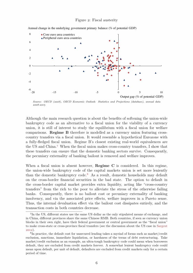
Figure 2: Fiscal austerity

Output gap (% of potential GDP)

-6

-4

-2

0

2

4

6

8

-20 -15 -10 -5 0 5 10

Core euro area countriesPeripheral euro area countries

Annual change in the underlying government primary balance (% of potential GDP)

Source: OECD (2018), OECD Economic Outlook: Statistics and Projections (database), annual data

2008-2017.

Although the main research question is about the benefits of softening the union-widebankruptcy code as an alternative to a fiscal union for the viability of a currencyunion, it is still of interest to study the equilibrium with a fiscal union for welfarecomparisons. Regime B therefore is modelled as a currency union featuring cross-country transfers via a fiscal union. It would resemble a hypothetical Eurozone witha fully-fledged fiscal union. Regime B’s closest existing real-world equivalences arethe US and China.7 When the fiscal union makes cross-country transfers, I show thatthese transfers can ensure that the domestic banking sectors survive. Consequently,the pecuniary externality of banking bailout is removed and welfare improves.

When a fiscal union is absent however, Regime C is considered. In this regime,the union-wide bankruptcy code of the capital markets union is set more lenientlythan the domestic bankruptcy code.8 As a result, domestic households may defaulton the cross-border financial securities in the bad state. The option to default inthe cross-border capital market provides extra liquidity, acting like “cross-countrytransfers” from the rich to the poor to alleviate the stress of the otherwise failingbanks. Consequently, there is no bailout cost or pecuniary externality of bankinginsolvency, and via the associated price effects, welfare improves in a Pareto sense.Thus, the internal devaluation effect via the bailout cost dissipates entirely, and thetransaction costs in both countries decrease.

7In the US, different states use the same US dollar as the only stipulated means of exchange, andin China, different provinces share the same Chinese RMB. Both countries, if seen as currency unionblocks in their own right, have their federal government or central government as the “fiscal union”to make cross-state or cross-province fiscal transfers (see the discussion about the US case in Sargent2012).

8In practice, the default cost for unsecured lending takes a myriad of forms such as market/creditexclusion, sanctions, immediate liquidation, or harshness of the terms of debt restructuring. Takemarket/credit exclusion as an example, an ultra-tough bankruptcy code could mean when borrowersdefault, they are excluded from credit markets forever. A somewhat lenient bankruptcy code couldmean upon default, per unit of default, defaulters are excluded from credit markets only for a certainperiod of time.

6

Nevertheless, a caveat of bankruptcy leniency remains: there exists a lower bound forthe union-wide bankruptcy code. If it is set too leniently, then for all states of nature,no households in the currency union would ever repay cross-border borrowing, andthe capital markets union would collapse. This scenario is inferior even to the internaldevaluation regime because such an ultra-lenient union-wide bankruptcy code impedescross-border risk sharing.

To corroborate the role of Regime C (bankruptcy leniency) in improving the via-bility of currency unions, the theory needs to explain why cross-border default viabankruptcy code adjustment is particularly vital for currency unions. To understandthis question, it is important to know what benefits a currency union has given up andwhether cross-border default can serve to recoup these benefits. Therefore, I extendthe model to consider currency union dissolution and national currencies, a questionlargely unaddressed in the existing literature.

Regime D is such an extension. It considers national currencies and competitive float-ing exchange rates. I prove that under very general conditions, competitive floatingexchanges indeed adjust for and neutralise domestic credit risks. Accordingly, bankssurvive and welfare improves. However, if a currency union is the a priori arrange-ment of member countries, in a parameterisation of the model I show that RegimeC (bankruptcy leniency) obviates such needs for floating exchange rates to neutralisedomestic credit risks. Essentially, removing nominal exchange rates implies rigiditiesin the country-level inflation. Since countries cannot rely on inflation as a form of“soft” default, the capital markets union should allow for actual default and acknowl-edge the underlying credit risks. Encouraging some degree of cross-border default bysoftening the union-wide bankruptcy code therefore provides a compensation for thelost benefits of nominal exchange rates.

The rest of the paper is structured as follows: Section 2 reviews the related literature.Section 3 presents the currency union model, various regime equilibrium analysesand the analytical results. Section 4 conducts a welfare and numerical analysis andprovides the impetus for policy considerations. Section 5 investigates the nationalcurrency case. Section 6 discusses the results, policy implications, and two layers ofinstitutional details (one on the Eurozone TARGET2 system and the other on thecross-border insolvency reforms in practice). Section 7 is a conclusion.

2 Related Literature

A burgeoning emergence of academic endeavour has started tackling this issue of cur-rency union viability.9 Broadly, there are three types of proposals, albeit not orthog-onal to one another and non-exhaustive: 1) fiscal unions (e.g., Farhi and Werning2017; Kehoe and Pastorino 2017), 2) banking unions (e.g.,Martinez et al. 2019), and3) union-wide safe assets (e.g., Brunnermeier et al. 2016). The welfare improvementhinges on whether these proposals can reduce transaction costs and improve risk shar-ing; however, pragmatically, the aforementioned proposals may encounter politicalresistance from nation states within the currency union. Therefore, the political eco-nomic consideration of these three proposals is likely to spark off further excitingresearch (see Foarta 2018). My work contributes to existing work by considering an

9See Brunnermeier and Reis (2015) for an excellent summary of recent theories.

7

alternative financial regime, i.e. capital markets union (see Martinez et al. 2019). Thekey step forward of my work is that I consider the economics of bankruptcy within thecapital markets union in the presence of credit risks, which are omitted in Martinezet al. (2019). This financial regime is plausible because the forces work through theinvisible hand of the markets, which might encounter less political resistance in termsof implementation.

My work is also related to the rich body of literature on optimal currency areas thatstarts with Mundell (1961); McKinnon (1963); Kenen (1969). Subsequently the newopen economy macro literature (salient examples include Obstfeld and Rogoff 2000;Gali and Monacelli 2005) builds micro-foundations and is applied to provide concretewelfare analysis on the monetary and fiscal issues in currency unions (see Gali andMonacelli 2008; Ferrero 2009; Aguiar et al. 2015; Farhi and Werning 2017; Kehoeand Pastorino 2017; Adam and Grill 2017). My work complements this body of lit-erature by introducing the finance elements and explicitly modelling the endogenousdetermination of the value of currencies. Moreover, I incorporate credit risks and moralhazard, which were at the forefront of the eurozone debt crisis. Rather than assum-ing a continuum of atomistic countries, I take the two-country international financeapproach, which is a suitable laboratory to analyse the north-and-south dynamics inthe Eurozone.

In terms of the broader message, my paper shares a similar kindred spirit to Adam andGrill (2017) and Goodhart et al. (2018) that cross-border default can conditionallybenefit currency unions. However, these two papers do not explain why cross-borderdefault is particularly vital to sustain a currency union. For example, the frictionin Adam and Grill (2017) is the non-state contingent bond, which is not necessarilya friction that is specific to currency unions. It is known in the general equilibriumtheory with incomplete markets that strategic default can improve risk sharing byincreasing the asset span (see Zame 1993; Dubey et al. 2005). Thus, the welfareimprovement result found in Adam and Grill (2017) is expected and should holdqualitatively, even assuming away currency unions. Different from Goodhart et al.(2018) and Adam and Grill (2017), my work explicitly models the arrangement ofsharing the common currency. Meanwhile, my model makes available state-contingentnominal financial securities in order to show that cross-border default is needed forrisk sharing due to being bound by the common currency in the presence of domesticcredit risks. Therefore, my model is able to conduct the counterfactual experiment oncurrency union dissolution and compare and contrast a currency union with the caseof national currencies and competitive flexible exchange rates.

To model a currency union with banking fragility (e.g. the Eurozone Crisis), themodel should explicitly include the currency, banks, liquidity, and credit. Therefore, Ichoose an international finance modelling framework based on the seminal papers byGeanakoplos and Tsomocos (2002); Tsomocos (2008); Peiris and Tsomocos (2015).Geanakoplos and Tsomocos (2002) model a general equilibrium to unify internationaltrade and finance. Their model is rich enough to include multiple goods, multiplecountries, multiple consumers in each country, multiple time periods, multiple creditmarkets, and multiple currencies. The authors prove the existence of the equilibrium.Because of the role of money and the heterogeneity of markets and agents, the authorsprove that fiscal and monetary policy both have real effects even under flexible prices.Parallel to Geanakoplos and Tsomocos (2002), Tsomocos (2008) proves generic de-

8

terminacy and money non-neutrality of international monetary equilibria. The authorobtains price-level determinacy and the endogenous determination of exchange ratesin a rich general equilibrium. Further enriching Geanakoplos and Tsomocos (2002),Peiris and Tsomocos (2015) develop an international finance model with incompletemarkets and relax the assumption of fully committed debt repayment. The authorsprove the equilibrium existence and obtain a non-trivial role for monetary policy withincomplete markets and credit risks. These frameworks incorporate money and finan-cial frictions into international trade, sharing a similar spirit to Manova (2012).

In this paper, I simplify and modify Peiris and Tsomocos (2015) to consider the specialcase of a currency union. Rather than assuming each country has one independentcentral bank as in Peiris and Tsomocos (2015), I assume that countries share the samecentral bank and I also consider the risk-shifting of domestic commercial banks, whichare not present in Peiris and Tsomocos (2015). These modifications allow me to isolatethe impact of sharing a common currency on the seigniorage split between domesticcommercial banks and the union-wide central bank (see Reis 2013).

Money and liquidity creation via bank credit are key features of this paper. This mech-anism was much emphasised by early economists when the banking sector was justbooming. Classic works by Macleod (1866), Wicksell (1906), Hahn (1920), Hawtrey(1923), Schumpeter (1954), Keynes (1931), Tobin (1963) and Minsky (1977) have allprovided insight into this monetary operation and its macro-financial implications.The early formalisation of this mechanism can be found in the general equilibriumtheory of money. In this literature, there is an assumed requirement that money mustbe used to carry out transactions formalised through cash-in-advance constraints simi-lar to Grandmont and Younes (1972, 1973); Lucas Jr and Stokey (1987). Inside moneyenters the economy against an offsetting obligation that guarantees its departure, andit is issued when borrowing agents apply for loans from the banks. As in Tsomocos(2003), commercial banks can be viewed as creators of “money” à la Tobin (1963).Some quantity of money, called outside money, is present as agents’ initial monetaryendowment that is used to pay for loan interest. The banking sector therefore can beeither an intermediary of existing money or a creator of new inside money, as in Dubeyand Geanakoplos (1992, 2003b, 2006), Bloise et al. (2005), Bloise and Polemarchakis(2006), Tsomocos (2003), and Goodhart et al. (2006, 2013).

Following the 2007-2009 Global Financial Crisis, there has been a revival of insidemoney modelling due to the renewed interest in banks’ balance sheet transformationfor credit extension and liquidity creation and the associated macro-financial outcomes.Recent advances include and are not limited to Bigio and Weill (2016), Brunnermeierand Sannikov (2016) , Faure and Gersbach (2017), Donaldson et al. (2018), Kumhofand Wang (2018), Bianchi and Bigio (2018), Piazzesi and Schneider (2018), McMahonet al. (2018), Kiyotaki and Moore (2018a), Kiyotaki and Moore (2018b), and Tsomocosand Wang (2019). Sharing a similar spirit to inside money provision against bankcredit, liquidity creation is also much emphasised in the literature on banking (seeGorton and Pennacchi 1990; Diamond and Rajan 2001; Stein 2012; Hart and Zingales2014; DeAngelo and Stulz 2015) and safe assets (see J Caballero and Farhi 2017).

In addition to banks and liquidity, the second key ingredient of my work is endogenousdefault, and it connects with a large body of literature on strategic sovereign default.Although I do not explicitly model the default decision by a separate government, in my

9

model the default decision of the atomistic households in a given country is interpretedas the aggregate default at the country level. Typically there are two ways of thinkingabout default at the country level: 1) strategic default via explicit default costs (e.g.Eaton and Gersovitz 1981; Aguiar and Gopinath 2006; Arellano 2008; Arellano andRamanarayanan 2012; Na et al. 2018 ) and 2) default without explicit costs but drivenby political considerations (e.g.Guembel and Sussman 2009; D’Erasmo and Mendoza2016). My paper belongs to the first group. As argued in Eaton and Gersovitz (1981),strategic default is suitable to analyse the trade-off of country-level default, becauseany negative net worth criterion for a country-level default is essentially irrelevant.

At the country level, default punishment can take a myriad of forms that range fromcredit or market exclusion (e.g. Eaton and Gersovitz 1981; Aguiar and Gopinath 2006;Arellano and Ramanarayanan 2012; Na et al. 2018) to sanctions (see the discussion inBulow and Rogoff 1989), and from the loss of insurance opportunities (e.g. Bloise et al.2017) to internal devaluation (e.g. Regime A of this paper). In light of this considera-tion, in this paper I do not model the various specific forms of punishment but assume anon-pecuniary default penalty à la Shubik and Wilson (1977) and Dubey et al. (2005).The intensity parameter λ of the default penalty is interpreted as the bankruptcy codein my model. Unlike Eaton and Gersovitz (1981); Aguiar and Gopinath (2006); Arel-lano and Ramanarayanan (2012); Na et al. (2018) that model default as a binarydecision, my paper emphasises that the social cost of default depends on the severityof default; hence, partial default is also considered. Modelling partial default is alsofound in Calvo (1988); Bolton and Jeanne (2007); Corsetti and Dedola (2013); Adamand Grill (2017) and is in line with empirical evidence (see Trebesch and Zabel 2017)and quantitative findings (see Gordon and Guerron-Quintana 2018). I acknowledgethat an alternative way of modelling default punishment would be to collateraliselending. However, because I model aggregate debt positions at a country level, seizing“collaterals” at a country level would imply further political frictions outside the scopeof this paper. In light of this issue, I have only considered uncollateralised lending.

Moreover, the model extension of this paper connects with the body of literature onthe cost and benefit of flexible exchange rates and the nexus between nominal exchangerates and default. For example, Neumeyer (1998) acknowledges that the general beliefthat “excessive” exchange rate variability harms the economy is difficult to prove ina formal setting. However, the author shows when the excess exchange rate risk isdriven by political factors that influence monetary affairs, flexible exchange rate causesinefficiency. Guembel and Sussman (2004) use a market microstructure approach toobtain optimal exchange rates, and the authors assume markets are incomplete so thatthe cost of flexible exchange rates stems from its volatility that impedes risk sharing.In the model extension of my paper in which national currencies are considered, Ideliberately choose not to model any cost of flexible exchange rates but only considerthe potential benefits. This is because I want to pin down the upper bound of the lostbenefits by removing nominal exchange rates and see how much cross-border default incurrency unions can recoup the lost benefits of flexible exchange rates. Indeed, a keybenefit of flexible exchange rate in my model extension is to neutralise domestic creditrisks such that banks remain solvent. The role of nominal exchange rate therefore isto provide a buffer for country-level default, an insight reminiscent of a key point fromUribe (2006).

Finally, as my modelling environment features agent heterogeneity, banking and liq-

10

uidity, and financial assets, it follows that default risk premium, rents extracted by thebanking sector, bailout costs, and the value of the currency all affect the stochasticdiscount factor (SDF) for asset pricing. The exact specification for SDF depends oneach regime considered. Such asset pricing formulae complement the growing body oftheoretical and empirical literature on intermediary asset pricing (see He and Krish-namurthy 2013; Adrian et al. 2014; He et al. 2017; Bongaerts et al. 2017; Kondor andVayanos 2019).

3 The Model - Currency Union

The model is a simple two-country endowment economy with uncertainty, and bothaggregate endowment risks and idiosyncratic income risks are present. There are twotypes of consumption goods available for international trade, and each country has onlyone type of consumption good. In each country reside a domestic commercial bankingsector and a continuum of households. A union-wide central bank acts as lender oflast resort of issuing the common currency to the two national commercial bankingsectors. The common currency is fiat because it does not enter utility functions.Households borrow from commercial banking sectors to obtain the common currencyfor transactions.

3.1 Model Description

The economy has three periods, t ∈ T = {0, 1, 2}, with date t = 1 having S states ofnature which I index with s ∈ S = {1, .., S}. Including date t = 0, there are S + 1date-events in the set S∗ = {0, 1, .., S}. Consumption happens at t = 0, 1, and datet = 2 is for any outstanding loan settlement. For simplicity there is no discounting.The two countries are indexed byH ∈ {I, J} where trade occurs at prices denominatedin a common currency. Country I has a measure 1 of households i and the commercialbanking sector i, and country J has a measure 1 of households j and the commercialbanking sector j.

Households in both countries are risk-averse and consumption goods are all perishable.In country I, households i are endowed with outside moneymi in the common currencyand domestic consumption good eiI0 at t = 0. At t = 1, households i are endowed withstate contingent domestic consumption goods eiI = (eiI1, .., eiIs, .., eiIS) ∈ RS

+. Similarly,in country J , households are endowed with outside money mj in the common currencyand domestic consumption good cjJ0 at t = 0. At t = 1, households j are endowedwith state contingent domestic consumption goods ejJ = (ejJ1, .., e

jJs, .., e

jJS) ∈ RS

+. Inevery state of nature, the two types of goods are traded at nominal spot prices pI =(pI0, pI1, ..., pIs, ...pIS) ∈ RS∗

+ and pJ = (pJ0, pJ1, ..., pJs, ..., pJS) ∈ RS∗+ in the common

currency. Given two types of contingent endowments and households’ preferences,both aggregate endowment risks and idiosyncratic income risks can be captured.

To link cross-country trade and capital flows, I make available state-contingent nominal

financial securities. These financial securities are akin to Arrow securities, but thepayoff of the financial security for state s is 1 unit of the common currency, ratherthan 1 unit of good I or J . I assume the number of these financial securities is the sameas the number of states, and I call these securities as the nominal Arrow securities. Theset of state prices is denoted as π = (π1, ..πl, .., πS) ∈ RS

+. These financial securitiesare traded on exchanges, so I have in mind this huge anonymous international capital

11

market in a currency union. Therefore, cross-country lenders and borrowers do nothave one-on-one interactions.

In addition to the financial contracts, there are inter-period domestic loan contractsand interbank loan contracts that provide liquidity in the common currency as theonly stipulated means of exchange. The union-wide central bank lends interbankloans (µiCB, µ

jCB) to provide the common currency to the commercial banking sectors

in the two countries. In each country, there is a domestic commercial bank sector thatextends loans (µiI or µ

jJ) to provide liquidity in the common currency to its respective

domestic households, as in Assumption 1.

Assumption 1 (bank lending). In terms of loans to non-bank sectors, commercial

banks only grant loans to domestic non-bank sectors, but not foreign non-bank sectors.

This assumption is based on the strong “home bias” of bank lending in the Eurozonewidely documented in empirical literature (see Acharya and Steffen 2015; Becker andIvashina 2017; Gabrieli and Labonne 2018; Ongena et al. 2018). It also reflects thedoom-loop in the Eurozone à la Brunnermeier et al. (2016) and Farhi and Tirole (2017)that banks in the eurozone hold disproportionately large amount of national debt orbonds issued by their own sovereigns.10

The capital markets union takes the form of financial asset markets that facilitate cross-country capital flow. Following Shubik and Wilson (1977) and Dubey et al. (2005),market participants choose how much to deliver for asset payoffs, and the asset marketis assumed an anonymous market with promises between different sellers not allowedto be distinguished even though they may deliver differently. This assumption impliesthat the expected delivery rates of the financial securities denoted as K are macrovariables taken as given by the households, in the same tradition as the competitivemarket environment. All deliveries are pooled and buyers of the pool for each financialsecurity receive a pro rata share of the net deliveries. Each ownership share of thepool of the financial security s receives a fraction Ks ∈ [0, 1] of the promised deliveryin state s.

10As many existing works have endogenised this home bias or relationship lending either in theeurozone context or in a broader context (see Acharya and Rajan 2013; Gennaioli et al. 2014; Uh-lig 2014; Acharya et al. 2014; Farhi and Tirole 2017); therefore, I do not seek to provide furthermicrofoundations for Assumption 1 in this paper.

12

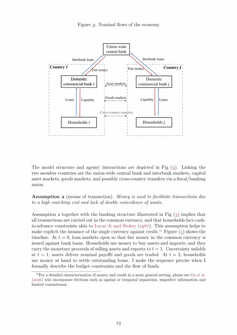
Figure 3: Nominal flows of the economy

Union-wide central bank

Domestic commercial bank �

Country � Country �

Domestic commercial bank �

Households � Households �

Interbank loans

Fiat money

Interbank loans

Fiat money

Loans Liquidity Liquidity Loans

Asset markets

Goods markets

Cross-country transfers

The model structure and agents’ interactions are depicted in Fig (3). Linking thetwo member countries are the union-wide central bank and interbank markets, capitalasset markets, goods markets, and possibly cross-country transfers via a fiscal/bankingunion.

Assumption 2 (means of transaction). Money is used to facilitate transactions due

to a high searching cost and lack of double coincidence of wants.

Assumption 2 together with the banking structure illustrated in Fig (3) implies thatall transactions are carried out in the common currency, and that households face cash-in-advance constraints akin to Lucas Jr and Stokey (1987). This assumption helps tomake explicit the issuance of the single currency against credit.11 Figure (4) shows thetimeline. At t = 0, loan markets open so that fiat money in the common currency isissued against bank loans. Households use money to buy assets and imports, and theycarry the monetary proceeds of selling assets and exports to t = 1. Uncertainty unfoldsat t = 1, assets deliver nominal payoffs and goods are traded. At t = 2, householdsuse money at hand to settle outstanding loans. I make the sequence precise when Iformally describe the budget constraints and the flow of funds.

11For a detailed characterisation of money and credit in a more general setting, please see Gu et al.(2016) who incorporate frictions such as spatial or temporal separation, imperfect information andlimited commitment.

13

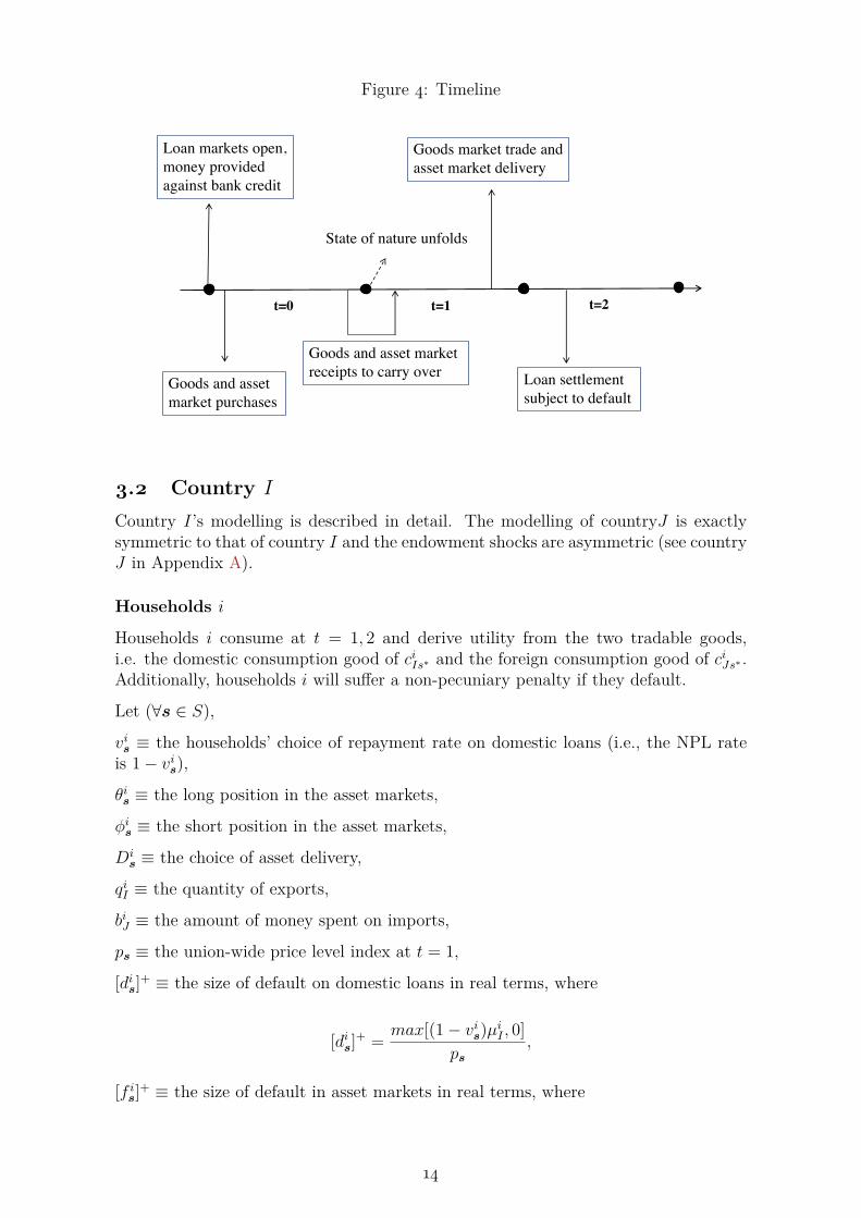
Figure 4: Timeline

Loan markets open, money provided against bank credit

State of nature unfolds

Goods market trade and asset market delivery

t=0 t=1

Goods and asset market receipts to carry over Loan settlement

subject to default Goods and asset market purchases

t=2

3.2 Country I

Country I’s modelling is described in detail. The modelling of countryJ is exactlysymmetric to that of country I and the endowment shocks are asymmetric (see countryJ in Appendix A).

Households i

Households i consume at t = 1, 2 and derive utility from the two tradable goods,i.e. the domestic consumption good of ciIs∗ and the foreign consumption good of ciJs∗ .Additionally, households i will suffer a non-pecuniary penalty if they default.

Let (∀s ∈ S),

vis ≡ the households’ choice of repayment rate on domestic loans (i.e., the NPL rateis 1− vis),

θis ≡ the long position in the asset markets,

φis ≡ the short position in the asset markets,

Dis ≡ the choice of asset delivery,

qiI ≡ the quantity of exports,

biJ ≡ the amount of money spent on imports,

ps ≡ the union-wide price level index at t = 1,

[dis]+ ≡ the size of default on domestic loans in real terms, where

[dis]+ = max[(1− vis)µiI , 0]ps

,

[f is]+ ≡ the size of default in asset markets in real terms, where

14

[f is]+ = max[φis −Dis, 0]

ps.

Formally households’ preference is given as follows:

Max︸ ︷︷ ︸µi

I ,θi,φi,ci

I ,ciJ ,q

iI ,b

iJ ,v

i,Di

E0

{U i(ciI0, c

iJ0, c

iIs, c

iJs

)− λi[dis]+ − λ[f is]+

},

where the preference over consumption goods U(·) is assumed to be homothetic, strictlyincreasing, concave, and differentiable. The disutility from default is separable fromconsumption utility and is linear in the amount of default. The λi denotes the domes-tic default penalty harshness, which is interpreted as the domestic bankruptcy codethroughout the paper. I denote the union-wide bankruptcy code as λ. Default can beeither strategic or due to ill fortune, but creditors cannot observe why borrowers de-fault. The households evaluate their own marginal benefit from default and marginalcost of default. If the former is larger than the latter, households default strategicallyeven if there are resources at hand.

Households i choose the amount of domestic loans of µiI to borrow, the quantity ofnominal Arrow securities of θi to buy, the quantity of nominal Arrow securities of φi tosell, the quantity of domestic goods of ciI to consume, the amount of importing goodsof ciJ to consume, the amount of exporting goods of qiI , the amount of money of biJ tospend on imports, the loan repayment rate of vi, and total asset delivery of Di.

Let ∆ denote any unused money from the corresponding flow of funds constraint, letηi0, η

i1s, η

i2s be the shadow price of the corresponding constraint, let rI be the domestic

loan rate and τIs be the domestic tax rate, let Ks be the aggregate delivery rates ofthe nominal Arrow security l = s, and let δis be any potential cross-country transfer.When a fiscal union is absent, then δis is simply set to 0 for all states. Households iare subject to the following budget sets and flow of funds constraints.

At t = 0:

biJ0 +S∑l=1

πlθil ≤

µiI1 + rI

+mi. ηi0 (1)

At t = 1 ∀s ∈ S:

biJs(1 + τIs) + (Dis −Ksθ

is) + φisτIs ≤ ∆(1) +

S∑l=1

πlφil + pI0q

iI0 + pIsq

iIs + δis. ηi1s (2)

At t = 2:

15

visµiI ≤ ∆(2)s. ηi2s (3)

And for s∗ ∈ S∗, the feasibility constraints are satisfied, i.e., ciIs∗ ≤ eiIs∗ − qiIs∗ andciJs∗ ≤

biJs∗pJs∗

.

Condition (1) states that at t = 0, households apply for an inter-period loan12 ofµiI from the domestic commercial banking sector at the loan rate rI to obtain insidemoney. Households i use the money inflow from the domestic commercial bankingsector, plus any outside money of mi to buy nominal Arrow securities and imports(money as a means of transaction). At the same time, households i receive monetaryincome from selling securities and exports for a total of ∑S

l=1 πlφil + pI0q

iI0 and carry

it over into t = 1 (money as a store of value).

Condition (2) states that at t = 1, households i use the monetary income from t = 0and export income of t = 1 plus any unused money ∆(1) and cross-country fiscaltransfer of δis (if any) to spend on the imports of biJs and to deliver the net monetarypayoff of Di

s − Ksθis for the security l = s. Moreover, import expenditures and

cross-country borrowing are subject to a state-contingent tax levied by the nationalgovernment for a possible bailout fund.

At t = 2, households use the residual money from t = 1 to settle the domestic loanand choose how much to repay or default (see Condition (3)). This loan settlementconstraint is equivalent to the transversality condition in infinite horizon models.

Domestic Commercial Banking Sector i

Bank i is the domestic commercial banking sector in country I. Bank i extends loansto domestic households and provides liquidity for the households to make purchases.To ensure the liquidity bank i provides would have a one-to-one convertibility to thecommon currency the union-wide central bank issues, bank i needs to borrow interbankloans from the union-wide central bank to meet the liquidity demands from domestichouseholds. In this sense, commercial banks act as the “creators of money” à la Tobin(1963), with the central bank being the ultimate fiat money issuer.13

Bank i needs to make the following choices. It needs to choose how much domesticliquidity of µiI/(1 + rI) to supply to the household, how much interbank loans µiCBto borrow from the union-wide central bank to obtain the fiat money denominated inthe common currency, how much interbank liquidity Li to make available to ensurethat the liquidity supplied to domestic households has a one-to-one convertibility tothe common currency obtained from the central bank. Bank i maximises its fran-chise value, defined as the average payoff across states weighted by the risk-neutralprobabilities. Formally,

12The modelling of the inter-period loan reflects the reality that the bank’s asset is typically lessliquid than its liability, i.e. money in this case.

13In practice, when individual commercial banks supply loans they immediately write deposits asIOU notes for the borrowers, but the deposits are convertible to central bank reserves with the centralbank being the lender of the last resort. Therefore, ultimately fiat money is issued by the centralbank, and the commercial banks are a risk-shifting “pass-through” of central bank fiat money.

16

Max︸ ︷︷ ︸µi

CB ,µiI ,L

i,ωi

S∑s=1

zsωis,

where ωis is bank i’s nominal profits for state s and zs is the risk-neutral probabilityfor state s. Let ρ be the interbank rate, and let Ri

s be the bank’s expected repaymentrate of the households. Bank i is subject to the following flow of funds constraints:

Li ≤ µiCB1 + ρ

, (4)

µiI1 + rI

≤ Li, (5)

ωis = ∆(4) + ∆(5) +Risµ

iI − µiCB. (6)

At t = 0, bank i borrows interbank loans from the union-wide central bank and obtainsfiat money in the common currency, ready to be extended as interbank liquidity of Li.This is shown in Condition (4).

Meanwhile when bank i extends commercial loans of µiI to the households, it mustensure the liquidity bank i provides against the bank loans has a one-to-one convert-ibility to the fiat money issued by the central bank. This is shown in Condition (5)and Lemma 2, which shall prove that Condition (5) is binding whenever ρ > 0. Eq(6) states at t = 2, ∀s ∈ S, bank i uses the households’ loan repayment to pay backthe interbank loans14 to the union-wide central bank, and the difference between thesetwo repayments adds to bank i’s net cash flow, i.e. profits.

Depending on the NPL rate of 1−vis for state s ∈ S, bank i’s nominal profits ωis couldbe negative and that bank i becomes insolvent. Given the characteristics of differentregimes to be specified in Proposition 2, there may be cross-country transfers of δbIsor domestic government bailout funds of TIs injected to bank i. I define ωi′s as theafter-bailout net cash inflow to bank i, ∀s ∈ S, i.e., ωi′s = ωis + δbIs + TIs.

National Government i

National government i collects taxes from domestic households to build a state-contingentbailout fund of TIs. Assumption 3 implies that national government will levy tax tobail out the domestic banking sector, should the government foresee domestic bankinginsolvency in a particular state. The households and the domestic commercial bankingsector are assumed uninformed at t = 0 of the national government’s contingent actionat t = 1. At t = 1, they take the government’s action as given.

Assumption 3 (bailout). The insolvency of the domestic banking sector incurs a high

social cost.

14Interbank loans are modelled as non-defautable. When the Euro Crisis emerged, the authoritiesarranged the form of the rescue to make sure that there was no default on the interbank loans thatFrench and German banks had provided to the Greeks.

17

The social cost in Assumption 3 can be interpreted in two dimensions. When thedomestic commercial banking sector incurs negative profits and becomes insolvent,it is unable to pay back the interbank loans to the union-wide central bank. Onedimension of the social cost is that domestic banking insolvency means defaulting onthe union-wide central bank. The implication is that the country as a whole may losethe membership of being in the currency union. The other dimension is that domesticbanking insolvency would require huge resources for the national government to restoreits domestic banking system. Given such considerations, the national government willbail out the domestic banking system should it foresee domestic banking insolvency ina certain state.

To collect the bailout fund, the national government levies taxes based on importexpenditures and cross-country borrowing as in Eq (7),15 reflecting the point that in abad state, the government resorts to fiscal austerity to bailout the domestic bankingsystem.

TIs = pJsciJsτIs + φisτIs. (7)

National government i uses the bailout funds to rescue the domestic commercialbanking sector whenever the banking sector’s nominal profits (adjusting for possi-ble cross-country transfers) would drop to negative, i.e. the bank fails. In short, inthe bad state the national government makes a state-contingent transfer to ensureωi′s = ωis + δbIs + TIs = 0.

3.3 Union-wide Central Bank

The union-wide central bank lends interbank loans of µhCB, ∀h ∈ {i, j}, and providesfiat money in the common currency to the two national commercial banking sectors.The union-wide central bank sets the interbank target rate of ρ as the policy rate.

To guarantee the determinacy of price level, the union-wide central bank, through theflow of funds of the banking system, collects households’ outside money as the seignior-age, but it does not redistribute the seigniorage within the same period. In this sense,the treatment of seigniorage in this model is non-Ricardian (Sims 1994; Buiter 1999).This approach follows Dubey and Geanakoplos (1992, 2006) and Tsomocos (2003). Itresonates the institutional separation between a central bank and a government, andtakes the view that price-level determinacy in equilibrium reflects the central bankmandate on price stability.

3.4 Equilibrium

The currency union equilibrium is defined as an allocation (ciIs∗ , ciJs∗ , cjIs∗ , c

jJs∗ , b

jIs∗ , b

iJs∗ ,

qiIs∗ , qjJs∗ , θ

hl , φ

hl , D

hs , µI , µJ , µCB) with prices (pIs∗ , pJs∗ , πl, rI , rJ , vhs , Rh

s), given bankru--ptcy codes (λh, λ) and policy rate and fiscal rules (ρ, τH , δh, δbH), ∀s∗ ∈ S∗, ∀s ∈ S,∀l ∈ S, h ∈ {i, j}, H ∈ {I, J} such that agents maximise subject to liquidity-in-advance constraints and budget constraints, markets clear, and expectations are ra-tional.

15Using tax rates rather than a lump-sum leads to clearer analytical expressions for propositions.The results are also robust to a lump-sum tax levy instead.

18

• Goods markets:pIs∗q

iIs∗ = bjIs∗ ,

pJs∗qjJs∗ = biJs∗ ,

• Asset markets for the nominal Arrow security s = l:∑h∈{i,j}

φhl =∑

h∈{i,j}θhl ,

• Domestic loan markets:

µhH1 + rH

= Lh,

• Interbank loan and money market:

1 + ρ = µiCB + µjCBM

,

• Rational expectation:

Ks =

∑

h∈{i,j}Dhs∑

h∈{i,j} φhs

if ∑h∈{i,j} φhs > 0

arbitrary if ∑h∈{i,j} φhs = 0

,

Rhs =

{vhs if 1− vhs > 0

arbitrary if 1− vhs = 0

}.

3.5 Equilibrium and Regime Characterisation

This subsection characterises the equilibrium and regimes. Suppose state s is a goodstate for country I and a bad state for country J , and state s′ is a bad state for countryI and a good state for country J , i.e. eiIs > eiIs′ , e

jJs < ejJs′ . The subsequent analysis

focuses on such asymmetric endowment shocks. Let γs the probability state s occurs,∀s ∈ S.

To ensure both nominal and real determinacy, Lemmas 1-3 prove the binding condi-tions of flow of funds constraints. Lemma 4 states the shadow price of the flow offunds constraint at t = 1. Lemma 5 and Proposition 1 characterise the equilibriumand Proposition 2 designs regimes of a currency union.

Lemma 1. Binding conditions of the Liquidity-in-advance constraints.

If rI > 0, then ∆(1) = 0.

If ρ > 0, then ∆(4) = 0.

Proof. See Appendix C.1.

19

Lemma 2. Interbank liquidity and the single currency convertibility.

If ρ > 0, then ∆(5) = 0.

Proof. See Appendix C.2.

Remark: That (5) binds means that the interbank liquidity the domestic bankingsector i extends to the households is pegged one-to-one to the common currency issuedby the union-wide central bank. This is not imposed a priori but rather a result ofthe non-arbitrage conditions from the interbank market.

Lemma 3. No worthless money at end.

If rI > 0, then ∆s(3) = 0.

If ρ > 0, then ∆s(6) = 0.

Proof. See Appendix C.3.

Lemma 4. Heterogeneous tightness of nominal constraints.

In a currency union with trades in goods market and asset market, if rI , rJ > 0 andno full default on loans, then ηi1s 6= ηi1s′ and/or η

j1s 6= ηj1s′ .

Proof. See Appendix C.4.

Lemma 5. (zero credit risks and the loss of exchange rate): If in the currencyunion ∀s ∈ S, h ∈ {i, j}, vhs = 1, given markets are complete, domestic bankingsectors break even for all states, i.e. ωhs = 0.

Proof. See Appendix C.5.

Claim. With domestic credit risks, the loss of floating nominal exchange rates (i.e.,

currency unions) translates into a currency crisis, disguised as a banking debt crisis,

i.e., ωhs < 0,∃s ∈ S, h ∈ {i, j}.

The above claim implies that the banking sectors in a currency union become morevulnerable due to losing the flexibility of exchange rates. Having a floating exchangerate might neutralise domestic credit risks and prevent such crises. Not to jump aheadof myself, I shall revisit this claim with a formal argument and proof in Proposition4 of the equilibrium analysis of the currency union and Proposition 6 in Section 5 inwhich I consider national currencies and the role of nominal exchange rates.

Given that in a currency union, zero domestic credit risks in all states of nature asin Lemma 5 is unlikely to hold in reality, in the subsequent analysis, I only focus onthe cases when domestic credit risks are present in a currency union. I also do notconsider the case of 100 % non-performing loans where there exists a state in whichthe household defaults on domestic loans completely. Formally, let,

Λh = {λh : vhs = 1, ∀s ∈ S, h ∈ {i, j}},

Λh = {λh : vhs = 0, ∃s ∈ S, h ∈ {i, j}}.

Thus, Λh covers the cases of full delivery of domestic loans in all states, and Λh covers

20

the cases in which there exists a state of full default on domestic loans. In all thesubsequent analysis I restrict λh to be an intermediate default penalty for domesticloans, i.e. for h ∈ {i, j}, λh /∈ Λh and λh /∈ Λh.

Proposition 1. (the Fisher effect, Quantity Theory of Money, and money

non-neutrality):

• The Fisher effect: Suppose for households i, biJs∗ > 0, ∀s∗ ∈ S∗. Supposefurther that households i have some money left over the moment the domesticloan comes due at s, then in equilibrium,

1 + rI =(E0(

U ici

Js

U ici

J0

)(pJ0

pJs) 1(1 + τIs)

)−1,

where U ici

J0and U i

ciJs

are household i’s marginal utilities of consuming imports att = 0 and in state s. A similar expression of the Fisher effect obtains for countryJ as well.

Taking the logarithm of the above Fisher equation and interpreting it loosely,the nominal interest rate equals the real interest rate plus the expected inflationadjusted by any bailout tax. Any tax needed for bank bailout in a currency unionalso distorts real allocation and inflation. As the bailout tax puts downwardpressure on inflation and the real interest rate, and it resembles fiscal austerity,I call this distortionary effect the internal devaluation effect.

• Quantity Theory of Money: If ρ > 0, the aggregate income of the currencyunion, namely the nominal value of consumption goods sales is equal to the totalstock of bank money and outside money, adjusted by asset trades and the bailouttax levy. Let ∆i

s = ∆(2)− pIsqiIs, and likewise for household j,

pI0qiI0 + pJ0q

jJ0 = M −

∑h∈{i,j}

S∑l=1

πlθhl +

∑h∈{i,j}

mh,

pIsqiIs + pJsq

jJs = M +

∑h∈{i,j}

mh −∑

H∈{I,J}THs −

∑h∈{i,j]

∆hs.

• Money non-neutrality: Suppose ρ > 0, any change in ρ results in a differentequilibrium in which some households’ consumption is different.

Remark: Even with flexible prices, money and default render monetary policy

non-neutral.

Proof. See Appendix C.6.

Corollary 1.1. (credit risks and the term-structure of interest rates): Supposeρ > 0, in a currency union with idiosyncratic credit risks, suppose vis >

∑Ss=1 zsv

is > vis′

and vjs <∑S

s=1 zsvjs < vjs′ , ∀s ∈ S, the term structure of interest rates incorporates

credit risks, and ωis, ωjs′ > 0.

21

In state s:

ρM + ( vjs∑Ss=1 zsv

js

− 1)µjCB + T js =∑

h∈{i,j}mh − ωis. (8)

In state s′:ρM + ( vis′∑S

s=1 zsvis

− 1)µiCB + T is′ =∑

h∈{i,j}mh − ωjs′ . (9)

Proof. See Appendix C.7.

Corollary 1.2. (Monetary policy rate pass-through): For H ∈ {I, J}, h ∈{i, j}, ∀s ∈ S,

1 + rH = 1 + ρ∑Ss=1 zsv

hs

. (10)

Corollary 1.1 states that both the liquidity creation by banks and the credit risksof households affect the term structure of the interest rates. The left-hand side ofthe Eqs (8) (9) is the union-wide central bank’s interest rate revenue for issuing thecommon currency. It equates the total outside money minus the rents extracted bycommercial banks, to be collected by the union-wide central bank at t = 2. Notethat the union-wide central bank does not collect all the outside money as profits.This amount of profits collected by the central bank is called seigniorage. No matterhow small it is, it serves to obtain price-level determinacy.16 Isomorphically, the termstructure of interest rate in relation to the seigniorage can be interpreted as the nexusbetween fiat money and the fiscal sovereign. Indeed, Goodhart (1998) argues thatseigniorage is part of the government’s taxation plan, and as Tsomocos (2003) puts it,by collecting the seigniorage, “the government compels the acceptance of fiat moneyas a final discharge of debt”.

Corollary 1.2 or Eq (10) shows the imperfect pass-through of the union-wide monetarypolicy hampered by credit risks. It states the borrowing cost at the national levelequates the union-wide monetary policy rate adjusted for the expected domestic NPLrates. The implication is that a fall in the union-wide monetary policy rate does notnecessarily translate to a loosened monetary condition at the national level, becausethe monetary policy pass-through is augmented with terms of financial contracts atthe national level.

Apart from the classic results above, the key step forward of this international financemodel is that it includes regime designs of a currency union by varying the domesticand cross-country bankruptcy codes (λh, λ, h ∈ {i, j}) and then their respective welfareproperties are ranked. Which regime the currency union falls under is endogenousto the relative harshness of domestic and union-wide bankruptcy code. In differentregimes, the terms in the term structure equations shall take on different values, andthe term structure equations summarise the driving force of the specific structural

16For a general proof of determinacy, please see Dubey and Geanakoplos (2006) and Tsomocos(2008).

22

assumptions in the various regimes considered. Proposition 2 formalises the regimedesign.

Proposition 2. (domestic and union-wide bankruptcy codes):

• If the union-wide bankruptcy code is harsher than the domestic bankruptcy code,households fully deliver on financial assets. i.e., for h ∈ {i, j},

– if λ > λh, Dhs = φhs at state s.

• If the union-wide bankruptcy code is more lenient, households may default onfinancial assets. i.e., for h ∈ {i, j},

– if λ < λh, 0 ≤ Dhs ≤ φhs at state s.

Proof. See Appendix C.8.

Proposition 2 states when the union-wide bankruptcy code is harsher than domesticbankruptcy codes, default in the cross-border capital markets does not occur; when thedomestic bankruptcy code is harsher than the union-wide bankruptcy code, default inthe cross-border capital markets may occur in equilibrium. Proposition 2 establishesthe foundation for the design of the following three regimes. Formally, define CAHsas country H’s current account net flow and FAHs as country H’s capital account netflow at t = 1, i.e.,

CAIs = pIsqiIs − pJsciJs,

FAIs = Ksθis −Di

s,

CAJs = pJsqjJs − pIsc

jIs,

FAJs = Ksθjs −Dj

s.

A positive CA means current account is running surplus and a positive FA meansinternational capital inflow, and vice versa. With these definitions, I state the followingregime designs.

• Regime A (baseline): λ > λh, δhs = δbHs = 0, THs = −ωhs whenever ωhs < 0,and THs = 0 whenever ωhs ≥ 0, where h ∈ {i, j}, H ∈ {I, J}, ∀s ∈ S.

Regime A is the baseline currency union in which a punitive union-wide bankruptcycode prevents default in the cross-border capital markets, and a fiscal union isalso ruled out. The domestic bailout tax is levied in the respective bad state tobailout the domestic banking system.

• Regime B (fiscal union): A currency union supported by a fiscal union, and apunitive union-wide bankruptcy code prevents default in the cross-border capitalmarkets, i.e., λ > λh, THs = 0, for h ∈ {i, j}, H ∈ {I, J}, ∀s ∈ S. I consider twocases for Regime B as follows.

– Regime B.a: A fiscal union that makes cross-country fiscal transfers ofδhs directly between households, and δhs = −FAHs − CAHs and δbHs = 0. It

23

follows that ∑h∈{i,j} δhs = 0.17

– Regime B.b: A fiscal union that makes cross-country fiscal transfer of δbHsdirectly between domestic commercial banks, such that ωhs + δbHs ≥ 0 and∑H∈{I,J} δ

bHs = 0, δhs = 0. Regime B.b can be interpreted as a banking

union supported by a common fiscal entity.

• Regime C (bankruptcy leniency): λ < λ < λh, δhs = δbHs = 0, and THs = 0.

Regime C is a currency union with a more lenient union-wide bankruptcy code,but a fiscal union is ruled out and no domestic bailout tax is levied. In thisregime, the bankruptcy code can induce endogenous default in the cross-bordercapital markets to emerge in equilibrium.

Note that the lower bound λ of the union-wide bankruptcy code in Regime C ensuresthe financial markets do not collapse. This is because if the union-wide bankruptcycode is too lenient, households in both countries would fully default on the financialassets; hence, assets would not be traded at t = 0. To sum up, Fig (5) illustratesthe regions of default penalty harshness and the corresponding regimes of the cur-rency union. The horizontal axis denotes the union-wide default penalty harshnessλ, the north-pointing vertical axis denotes domestic default penalty harshness λi andλj. For the ease of illustration, λi = λj, but the equality does not need to hold ingeneral. Focusing on the intermediate domestic default penalty harshness, Regime Cbelongs to the region where domestic bankruptcy codes are harsher than the union-wide bankruptcy code, and Regimes A and B belong to the region where the union-widebankruptcy code is tougher than domestic bankruptcy codes.

Figure 5: Regimes and bankruptcy codes

�

�� ��

Regime A &BRegime C

���

��

�

3.6 Equilibrium Analysis

In this subsection, I show the welfare properties of each regime for allocations, risksharing, and asset prices. In particular, propositions are given demonstrating themechanism in which a lenient bankruptcy code for the capital markets union couldimprove welfare. A caveat is also given that if certain conditions are not met, thepossibility of cross-border default could impede international risk sharing.

17Note that country H’s Balance of Payment (BoPHs ) in state s is BoPH

s = CAHs + FAH

s + δhs .

24

The intuition of the potential benefit of cross-border default in the capital marketsis that it provides extra liquidity for the borrower in the bad state such that risksharing improves. Before formalising welfare improvement, we need to understand themechanism how a lenient union-wide bankruptcy code can incentivise the borrower tograb the option to strategically default in the bad state. Suppose we are in RegimeC with a relatively lenient cross-country bankruptcy code. The households in the badstate may fully default on its cross-country borrowing whereas the other householdsin the other country may fully repay, if they both have short positions on the Arrowsecurity of this state. This is because the poor households have a high marginal utilityof consumption, which would outweigh the marginal cost of default on Arrow securities,given a lenient cross-country bankruptcy code. However, the other households are richin this state, and the marginal utility of consumption is low, which would push downthe marginal benefit of default. When the marginal benefit of default is less thanthe marginal cost of default, this rich households would fully deliver despite the poorhouseholds’ full default. Therefore, although the poor households would fully default,the aggregate default rate on the nominal Arrow security of that state actually wouldfall between 0 and 1.

Moreover, the poor households may enter both the short and long positions of thenominal Arrow security of the bad state. The poor households would buy this Arrowsecurity to insure against the bad shock, but they may also sell this Arrow securityat the same time because selling gives the option to default fully. The option todefault on Arrow securities provides extra liquidity leading to a possible increase inconsumption or a higher domestic loan repayment rate. This implies an increase inthe households’ utility. An interior solution can be obtained because although sellingmore of the Arrow security leads to extra liquidity due to default on the one hand,it implies this poor households would also need to buy more of this Arrow securitysuch that market clears, and buying on the other hand incurs more cost of liquidity.Proposition 3 formalises the mechanism of cross-border default. Later on, Proposition5 builds on Proposition 3 and proves Pareto improvement as a result of endogenousdefault in the cross-border capital markets.

Proposition 3. (strategic default on financial securities):

• When the union-wide bankruptcy code is lenient enough, households in the badstate may long and short the Arrow security of that state at the same time, andfully default on this Arrow security.

• Consider the case where S = {1, 2}, let γ1 = γ2, ei1 > ei2, and ej1 < ej2. Suppose

that in equilibrium λ < p2ηi12 < λi, ηj12 < λ

p2and ηi11 < ηi12 holds. Then,

φi2, φj2, θ

i2 > 0, θj2 = 0, Di

2 = 0, Dj2 = φj2, and 0 < K2 < 1 whenever

(K2 −

π2(vi2(1 + rI)− 1

))/pI2 > π2rI/pI1. Similar logic follows for the other state.18

Proof. See Appendix D.1.

Corollary 3.1. When the union-wide bankruptcy code is too lenient, it impedesinternational risk sharing in the currency union.

Corollary 3.2. As domestic bankruptcy codes become more lenient, the room to18In Section 4, an equilibrium with these characteristics is obtained.

25

adjust the union-wide bankruptcy code in the capital markets union decreases.

The insight of Proposition 3 is reminiscent of Example 2 in Dubey et al. (2005). Alenient cross-country bankruptcy code encourages the households in the bad state todefault fully. Even though the poor households have nominal inflows on hand fordelivery, they do not deliver anything while the rich households deliver fully! Defaultin this case is strategic and makes asset payoffs endogenous. Assets are still tradeddespite strategic default: the households in the poor country enter both long and shortpositions of Arrow securities and the households in the rich country only shorts Arrowsecurities of that state.

Note that financial securities are voluntarily traded despite the possibility of default,and no market participants are forced to buy or sell the financial securities. In thissense, the invisible hand of the markets provides “voluntary liquidity transfers” viaendogenous default. This mechanism is in principle different from Regime B where afiscal union employs a visible hand to move nominal resources directly. However, acaveat remains for Regime C (Corollary 3.1). Suppose now the union-wide bankruptcycode λ is set ultra-low, i.e. λ < ps′η

j1s′ or λ < psη

i1s, then Arrow securities are not

traded. The currency union loses risk sharing altogether. Therefore, there exist alower bound and an upper bound for the union-wide bankruptcy code of the capitalmarkets union.

Moreover, for the currency union to retain risk sharing and for the aforementioneddefault to occur in the cross-border capital markets in equilibrium, the union-widebankruptcy code λmust fall into the interval (ps′ηj1s′ , λi)∩(psηi1s, λ

j

as) in equilibrium. As

the domestic bankruptcy code λi or λj decrease, ||(ps′ηj1s′ , λi) ∩ (psηi1s, λj)|| decreases.Thus, as domestic bankruptcy codes become more lenient, the range to set cross-country bankruptcy code shrinks (Corollary 3.2).

A key condition for Proposition 3 to go through is ηj12 <λp2

in equilibrium (and itsequivalent for state 1), which says the union-wide bankruptcy code is strict enough toprevent default of the rich households. This condition ensures that defaultable Arrowsecurities are still traded in equilibrium even when the households of the poor countryin the bad state fully defaults. I call this condition within-union standard. When thetwo countries’ fundamentals differ exceptionally or when domestic bankruptcy code(s)are too lenient or discretionary, the “within-union standard” may fail to satisfy. Inthis case Regime C causes asset trades to collapse.

In contrast to Regime C, Regime B.a and Regime B.b advocate using the visible handof a common fiscal entity to make cross-country transfers. Whereas a fully-fledgedfiscal union in a currency union may be highly controversial and politically infeasible,in practice, there have been small steps towards building union-wide transfer funds, forexample, the concept of a banking union in the Eurozone. Therefore, it is of interestto investigate the properties of Regimes B.a and B.b.

Let var(1 − vh,B.as ) be the variance of non-performing loan rate of households h inRegime B.a, let var(1−vh,B.bs ) be that of households h in Regime B.b, and var(1−vh,As )that of Regime A, where h ∈ {i, j}. Lemma 6 says the domestic credit risk volatilityacross states is smaller in Regime B.a than in Regime B.b and Regime A.

26

Lemma 6 (credit risk volatility):

• A fiscal union that mediates transfers between households can reduce domesticcredit risk volatility across states.

• In Regime B.a, for h ∈ {i, j}, H ∈ {I, J}, suppose δhs = −FAHs −CAHs , it followsthat δis + δjs = 0, and moreover,

var(1− vh,B.as ) ≤ var(1− vh,B.bs ),

var(1− vh,B.as ) ≤ var(1− vh,As ).

Proof. See Appendix D.3.

Proposition 3 and Lemma 6 equip the currency union with distinct institutional fea-tures for the common objective to reduce domestic banking stress. Proposition 4formalises the mechanisms whereby this objective is achieved.

Proposition 4. (capital flow and banking crisis): Suppose λh /∈ Λh and λh /∈ Λh,for h ∈ {i, j}, H ∈ {I, J}, ∀s ∈ S.

• In Regime A, the volatility of domestic credit risks and international capital flowcan lead to domestic banking insolvency.

– If λ > λh and δhs = δbHs = 0, whenever vhs <∑S

s=1 zsvhs , then ωhs < 0 and

THs = −ωhs .

• In Regime B.a, international capital flow does not drive domestic banking insol-vency.

– If λ > λh, δbHs = 0, and THs = 0, setting δhs = −FAHs −CAHs , then ωhs = 0.

• In Regime B.b, the banking union funds alleviate domestic banking stress.

– If λ > λh, δhs = 0, and THs = 0, as long as ωjs + ωis ≥ 0, a banking unionfund of δbHs can be set to transfer between bank i and bank j such thatωhs + δbHs ≥ 0 and ∑H∈{I,J} δ

bHs = 0.

• In Regime C, default in the cross-border capital markets may prevent domesticbanking insolvency.

– If λ < λ < λh, δhs = δbHs = 0, and THs = 0, under the conditions inProposition 3 on strategic default, ωhs = 0.

Proof. See Appendix D.4.

Corollary 4.1. Under Proposition 4, Regimes B and C obviate the need for nationalbailout taxes whereas Regime A needs it.

Proposition 4 shows whether international capital flow may lead to domestic bankingstress under various regimes in a currency union. In Regime A, if domestic bailoutfunds are unavailable, the domestic commercial banking sector fails in the bad state.

27

In Regime B.a, the visible hand of a fiscal union sets the amount of cross-country fiscaltransfers mediated directly between households in different countries. Such transfersremove the stress from capital flow on member countries’ domestic banking system.Domestic commercial banks survive even in the bad state. In Regime B.b, the fiscalunion makes transfers directly between commercial banks of different countries, subjectto the total banking union fund constraint ωis +ωjs ≥ 0. However, Regime B.a faces nosuch constraint. This constraint is in line with Bolton and Oehmke (2018) that studybank resolution of global banks and show that the loss-absorbing capital is sharedacross jurisdictions but faces implementation constraints.

In Regime C, despite cross-country fiscal transfers being unavailable, a softened union-wide bankruptcy code can help domestic banks bypass the pressure from internationalcapital flow such that banks survive. The intuition is that a softened union-widebankruptcy code gives the domestic households the choice to default on their cross-country borrowing in the bad state. Because the domestic bankruptcy code is tougherthan the union-wide bankruptcy code in this regime, the marginal cost of default ondomestic bank loans is higher than the household’s marginal benefit of default. Ra-tionally, the households choose not to default on domestic loans even in the bad state.The takeaway is the relative stance of domestic and cross-country bankruptcy codescan change incentives on the margin and shift domestic credit risks to internationalcapital markets, relieving domestic banks from distress. Adjusting the union-widebankruptcy code, cross-border default provides a “voluntary” liquidity transfer viathe capital markets, in the absence of a fiscal union.

With different extent of domestic banking stress and accordingly distinct needs fornational level bailout tax, the regimes designed above bear different implications forallocation efficiency, risk sharing and asset prices. Under the conditions of Propositions3 and 4, the corollaries below formalise these implications for h ∈ {i, j}.

Corollary 4.2 (allocation efficiency within state):

• In Regime A, optimal allocation does not obtain in t = 0 due to domestic creditrisks and the cost of liquidity; optimal allocation within state does not obtain int = 1 due to the national bailout tax causing the internal devaluation effect.

At t = 0,

U ici

I0

U ici

J0

=U j

cjI0

U j

cjJ0

1(1 + rI)(1 + rJ) ,

and at t = 1, s ∈ S

U ici

Is

U ici

Js

=U j

cjIs

U j

cjJs

1(1 + τIs)(1 + τJs)

.

• In Regime B, optimal allocation efficiency does not obtain at t = 0 due todomestic credit risks and the cost of liquidity; optimal allocation within stateobtains at t = 1.

28

At t = 0,

U ici

I0

U ici

J0

=U j

cjI0

U j

cjJ0

1(1 + rI)(1 + rJ) ,

and at t = 1, s ∈ S

U ici

Is

U ici

Js

=U j

cjIs

U j

cjJs

.

• In Regime C, default in the cross-border capital markets obviates the need fornational bailout tax, optimal allocation does not obtain at t = 0 due to the costof interbank liquidity; optimal allocation within state obtains at t = 1.

At t = 0,

U ici

I0

U ici

J0

=U j

cjI0

U j

cjJ0

1(1 + ρ)2 ,

and at t = 1, s ∈ S

U ici

Is

U ici

Js

=U j

cjIs

U j

cjJs

.

Proof. See Appendix D.5.

We can observe that the wedge between the households’ marginal rate of substitutionacross goods distorts allocation efficiency within state. Regime A has the highest wedgedue to domestic borrowing costs and bailout tax rates, and the domestic borrowing costincorporates the cost of liquidity and commands domestic credit risk premia. RegimeC has the lowest wedge only resulting from the interbank transaction cost. Note thatthe transaction cost of money is Regime C is just the interbank transaction cost, andit is lower than the borrowing cost in Regime B. This is because the borrowing cost inRegime B commands the credit risk premium of domestic loans, but that of RegimeC precludes it owing to the shield of default in the cross-border capital markets.

Corollary 4.3. (risk sharing):

• In Regime A, optimal risk sharing does not obtain due to domestic credit risks,the cost of liquidity, and the bailout tax.

U ici

Is

U ici

Is′

=U j

cjIs

U j

cj

Is′

1(1 + τJs)(1 + τIs)(1 + rI)(1 + rJ) ,

29

U ici

Js

U ici

Js′

=U j

cjJs

U j

cj

Js′

1(1 + τIs′)(1 + τJs′)(1 + rI)(1 + rJ) .

• In Regime B, optimal risk sharing does not obtain due to borrowing costs whichcommands the domestic credit risk premium and incorporates the cost of liquid-ity.

U ici

Is

U ici

Is′

=U j

cjIs

U j

cj

Is′

1(1 + rI)(1 + rJ) ,

U ici

Js

U ici

Js′

=U j

cjJs

U j

cj

Js′

1(1 + rI)(1 + rJ) .

• In Regime C when default in the cross-border capital markets obviates the needfor national bailout tax, optimal risk sharing does not obtain due to two sourcesof inefficiency: the cost of interbank liquidity and the default premium in thecapital markets union.

U ici

Is

U ici

Is′

=U j

cjIs

U j

cj

Is′

KsKs′

(1 + ρ)2 ,

U ici

Js

U ici

Js′

=U j

cjJs

U j

cj

Js′

KsKs′

(1 + ρ)2 .

Proof. See Appendix D.6.

The above expressions tell us that the wedge between the households’ marginal rate ofsubstitution across states distorts risk sharing, and that the wedge in Regime A is thehighest because of the extra distortion stemming from the bailout tax. Between RegimeB and Regime C, however, it is not obvious whose wedge is higher. Both wedges inthese two regimes incorporate the interbank transaction cost and credit/default riskpremia.

Corollary 4.4. (asset prices): Financial, monetary, and fiscal factors all affect thestochastic discount factor.

• In Regime A, state prices are affected by the domestic credit risks, the cost ofliquidity, and the bailout tax directly.

πs = γsU ici

Js/pJs

U ici

I0/pI0

= γsU j

cjIs

/pIs

U j

cjJ0/pJ0(1 + τJs)(1 + rJ)

,

30

πs′ = γs′U ici

Js′/pJs′

U ici

I0/pI0(1 + τIs′)(1 + rI)

= γs′U j

cj

Is′/pIs′

U j

cjJ0/pJ0

.

• In Regime B state prices are only directly affected by the domestic credit risksand the cost of liquidity.

πs = γsU ici

Js/pJs

U ici

I0/pI0

= γsU j

cjIs

/pIs

U j

cjJ0/pJ0(1 + rJ)

,

πs′ = γs′U ici

Js′/pJs′

U ici

I0/pI0(1 + rI)

= γs′U j

cj

Is′/pIs′

U j

cjJ0/pJ0

.

• In Regime C state prices are affected by the interbank transaction cost and thecross-border default premium directly.

πs = γsU ici

Js/pJs

U ici

I0/pI0

= γsU j

cjIs

/pIsKs

U j

cjJ0/pJ0(1 + ρ)

,

πs′ = γs′U ici

Js′/pJs′Ks′

U ici

I0/pI0(1 + ρ) = γs′

U j

cj

Is′/pIs′

U j

cjJ0/pJ0

.

Proof. See Appendix D.7.

Asset prices are typically suppressed by the transaction wedge. The interbank trans-action cost, domestic loan credit risk premium, cross-border default premium, and thebailout tax all constitute the transaction wedge. We can observe from Corollary 4.4that the state prices in Regime A are typically lower than those in Regime B andRegime C, because Regime A is distorted by the bailout tax as the extra transactionwedge. Since the total transaction cost in Regime A is the highest, in this regimeone unit of currency tomorrow is worth the lowest level of consumption goods today.Thus, using internal devaluation to sustain a currency union would also put downwardpressure on asset prices. This is confirmed by the numerical analysis in Section 4.2.

4 Welfare and Numerical Analysis

4.1 Default and Welfare

The analysis so far suggests that both cross-country transfers and default in the capitalmarkets union can reduce the transaction wedge distorting allocations and prices.Table 1 provides a summary of the transaction wedge in Corollaries 4.1-4.4. The dash“-” indicates the relative degree of inefficiency. The more dashes assigned, there aremore sources of distortions to allocations, risk sharing, and asset prices.

31

Table 1: Regime comparison

Regime A Regime B Regime C

benchmark fiscal union default

Allocation within state - - - - - -

Risk sharing - - - - -

Asset prices - - - - -

Austerity tax yes no noBanking crises yes no noa “-” indicates the relative degree of inefficiency.

Let us observe that compared with Regime A, Regime C’s allocations, risk sharing,and asset prices are all much less distorted. This is because bankruptcy leniencyin the capital markets union can reduce the transaction cost for both countries inthe currency union; thus, naturally one expects Pareto improvement. Proposition 5formalises this claim.

Proposition 5. (Endogenous default and Pareto improvement):

• In the absence of a fiscal union, endogenous cross-border default can Paretoimprove a currency union.

• Consider the case where S = {1, 2}, let γ1 = γ2, ei1 > ei2, and ej1 < ej2. Consider

Regime A equilibrium, i.e. λi, λj < λ and vi2, vj1 < 1. Now reduce λ to λ

′

such that λi, λj > λ′ , whenever

(1 − π2

(vi2(1 + rI) − 1

))/pI2 > π2rI/pI1 and(

1 − π1(vj1(1 + rJ) − 1

))/pJ1 > π1rJ/pJ2, it leads to a utility increase for both

households i and j on the margin, while the expected utilities of domestic bankingsectors remain unchanged.

Proof. See Appendix D.8.

Interestingly, the philosophy underpinning the Pareto improvement here is to intro-duce an additional friction. Typically when a friction is added, there is one moreimperfection, and one might expect a worse outcome. Here, it is exactly the opposite.A currency union typically bear two imperfections: the interbank transaction costof money and the possibility to default on domestic loans, i.e. domestic credit risks.Suppose removing these two imperfections using brutal force is not possible, Regime Csimply introduces the possibility to default on financial assets as a third imperfection.The third imperfection is introduced in such a way that the most “harmful” imperfec-tion, i.e. state-varying domestic credit risks, is simply not manifested in equilibrium,leading to a superior outcome. Indeed, the possibility to default on financial assets canexactly shift borrowers’ incentive on the margin to bypass the state-varying domesticcredit risks, such that banks survive and no bailout tax is levied, as in Regime C.

I hasten to add that the conditions identified in Proposition 5 are only sufficient butnot necessary. The proof of Proposition 5 does not require setting the bailout taxrate to zero, which would provide an additional liquidity boost at t = 1 and increaseconsumption. However, as the softened bankruptcy code shifts the default incentive onthe margin, eventually the economy shifts to Regime C equilibrium where the bailout

32

tax is not even needed. Therefore, one can expect to further relax the conditions inProposition 5 for Pareto improvement to occur. As analytic solutions are not available,the exact sufficient and necessary conditions are difficult to pin down. Therefore, Iprovide numerical analysis in the next subsection.

4.2 Numerical Analysis

This subsection assumes two states (state s and state s′) in t = 1 and solves the modelnumerically. Table 2 exhibits the exogenous parameters and functional forms.

Table 2: Exogenous variables

Preference U i = αi0ln(ciI0) + (1− ai0)ln(ciJ0) + βiE0[αisln(ciIs) + (1− ais)ln(ciJs)]U j = αj0ln(cjJ0) + (1− aj0)ln(cjI0) + βjE0[αjsln(cjJs) + (1− ajs)ln(cjIs)]αi0 = αj0 = 0.5 αis = αjs′ = 0.7 αis′ = αjs = 0.3

Prob. of states γs = γs′ = 0.5Discount factor βi = βj = 1Endowment eiI0 = ejJ0 = 10 eiIs = ejJs′ = 15 eiIs′ = ejJs = 5Bankruptcy code λi = λj = 0.1036 λC = 0.098 λA = λB = 0.12Outside money mi = mj = 0.1Policy rate ρ = 0.01

4.2.1 Cross-border Default and Pareto Improvement

Table 3 shows the numerical solutions of the endogenous variables of Regime A,Regimes B.a and B.b, and Regime C.19 Let W I denote country I’s utility of consum-ing goods in both periods, SU I denote country I’s social utility, i.e. the consumptionutility minus the social cost of default, and df denote the default rate. Regime A leadsto the least desirable equilibrium among the four regimes considered: the default rateon domestic loans in the bad state is high, asset prices are suppressed, domestic com-mercial bank loan rates are much higher than the policy rate due to a high creditrisk premium, and bailout tax turns out positive as the domestic bank would becomeinsolvent in the bad state. Hence, both the allocation welfare and social utility ofRegime A are quite low.

19As country J is symmetric to country I, here I only display the prices and allocations of countryI for conciseness.

33

Table 3: Endogenous variables

Regime A Equilibrium (Baseline)W I = 3.2921 SU I = 3.2496 df i

s′ = 13.02% πs = 0.4807 rI = 8.03% τIs′ = 6.45%

Regime B.a EquilibriumW I = 3.2943 ↑ SU I = 3.2879 ↑ df i

s = 3.8% ↓ πs = 0.4875 ↑ rI = 4.49% ↓ τIs′ = 0% ↓

Regime B.b EquilibriumW I = 3.2943 ↑ SU I = 3.2711 ↑ df i

s′ = 6.75% ↓ πs = 0.4889 ↑ rI = 4.53% ↓ τIs′ = 0% ↓

Regime C EquilibriumW I = 3.2947 ↑ SU I = 3.2916 ↑ dfs′ = 1.63% ↓ πs = 0.4934 ↑ rI = 1% ↓ τIs′ = 0% ↓a Arrows indicate the direction of travel compared with Regime A.

Regime B.a is a fiscal union with no banking union. Default rates on domestic loansare the same across states, and are lower than Regime A, the internal devaluationregime; hence, the domestic commercial bank loan rates are lower. Moreover, assetprices, social utility and allocation welfare all improve upon Regime A, and the bailouttax is not needed. Regime B.b, a fiscal union with a banking union, exhibits a similarimprovement as Regime B.a.

Regime C assumes away cross-country fiscal transfers but a lenient union-wide bankruptcycode allows for cross-border default in the capital markets. In Regime C, the defaultrate is of asset payoffs and it is significantly lower than the default rate on domesticloans in Regime A. Since the cross-country bankruptcy code induces the default risksto move away from domestic loans for the purpose of alleviating domestic bankingstress, the domestic loan rate is equal to the monetary policy rate. Similar to RegimeB.a and Regime B.b, allocation welfare, social utility, and asset prices are all higherthan in Regime A, and the bailout tax is also not needed in Regime C.

Figure 6: Allocation welfare (shock variance)

14.65(5.35) 14.76(5.24) 14.87(5.13) 14.98(5.02) 15.09(4.91) 15.2(4.8)3.286

3.288

3.29

3.292

3.294

3.296

3.298

3.3

5.35(14.65) 5.24(14.76) 5.13(14.87) 5.02(14.98) 4.91(15.09) 4.8(15.2)3.286

3.288

3.29

3.292

3.294

3.296

3.298

3.3

Internal devaluationFiscal & banking unionCross-country default

Figure 6 conducts the robustness check of the numerical solution in Table 3 by varyingincome risks around the initial parameterisation of ehHs(h ∈ {i, j}, H ∈ {I, J}) set out

34

in Table 2. The horizontal axis represents the state-contingent endowments of thetwo states in each country. The further to the right, the greater the variance of thestate-contingent endowments while the mean remains unchanged at 10. The verticalaxis represents the households’ utility from consuming home and foreign goods, whichI call allocation welfare. As might be expected, Regime C with cross-border default inthe capital markets union Pareto dominates the Regime A which suffers from internaldevaluation. Regime B.b, the fiscal-banking union, is superior to Regime A as well butis slightly worse off than Regime C. This is because the transaction cost due to defaulton financial securities is lower than the transaction cost due to default on commercialbank loans.

Interestingly, as the variance of state-contingent endowments widens, the welfare im-provement of Regime C upon Regime A decreases. This is due to the substitutioneffect between default and consumption goods being dominated by the income effect,which reduces default risks in Regime A equilibrium. The widening variance impliesa lower endowment in the bad state, a higher marginal benefit of defaulting on do-mestic loans. The substitution effect thus would increase default rate. Meanwhile,a lower endowment in the bad state increases the value of this good and its relativeprice increases, which leads to an increase in liquidity inflow from goods sale to repaydomestic bank loans. Default rate hence decreases. The overall decrease in defaultrates push down the borrowing costs and the bailout tax rates in Regime A. Thus,Regime A’s allocation welfare deteriorates less as the variance widens, and the gapbetween Regime A and Regime C narrows. Adjusting the allocation welfare with thesocial cost of default, Figure 13 in Appendix E.1 replaces the vertical axis with socialutility (i.e. consumption utility minus the social cost of default) and shows a similarpicture. For more robustness check, I also replace the horizontal axis with country I’sstate 2 endowment eiI2 and shock the economy asymmetrically. Figure 14 in AppendixE.2 displays the social utility of both countries while changing eiI2. Again, cross-borderdefault Pareto improves upon the internal devaluation regime.

4.2.2 When Does Cross-border Default Not Work?

Nevertheless, a caveat remains on the welfare improving role of default in the cross-border capital markets. As Corollary 3.1 states, when the union-wide bankruptcycode λ is set too low, no households in either countries would ever repay cross-countryborrowing, leading to a collapse of international financial markets. Figure 7 providesnumerical support to this claim. As in Figure 6, the horizontal axis represents thestate-contingent endowments of the two states in each country. The solid line repre-sents the economy when the union-wide bankruptcy code is set to 0.098, only slightlymore lenient than the domestic bankruptcy codes (λh = 0.1036, h ∈ {i, j}). Thedashed line shows the economic allocation and prices when the union-wide bankruptcycode is set to 0.12, much tougher than the domestic bankruptcy codes. The dashedline essentially represents Regime A. The dash-dotted line represents financial au-tarky, where an ultra-low union-wide bankruptcy code (λ = 0.05) causes the collapseof financial markets and impedes risk sharing.

35

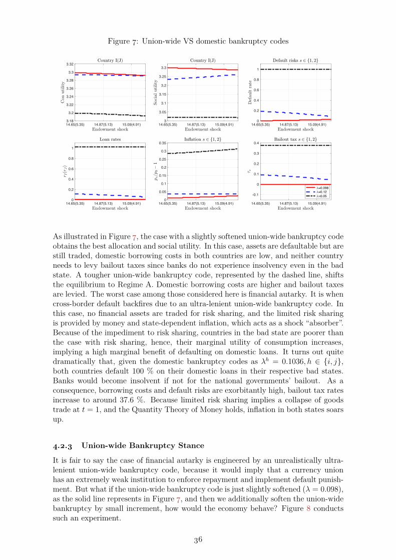
Figure 7: Union-wide VS domestic bankruptcy codes

14.65(5.35) 14.87(5.13) 15.09(4.91)3.18

3.2

3.22

3.24

3.26

3.28

3.3

3.32

14.65(5.35) 14.87(5.13) 15.09(4.91)3

3.05

3.1

3.15

3.2

3.25

3.3

14.65(5.35) 14.87(5.13) 15.09(4.91)0

0.2

0.4

0.6

0.8

1

14.65(5.35) 14.87(5.13) 15.09(4.91)0

0.2

0.4

0.6

0.8

1

14.65(5.35) 14.87(5.13) 15.09(4.91)0

0.05

0.1

0.15

0.2

0.25

0.3

0.35

14.65(5.35) 14.87(5.13) 15.09(4.91)

-0.1

0

0.1

0.2

0.3

0.4

=0.098=0.12=0.05

As illustrated in Figure 7, the case with a slightly softened union-wide bankruptcy codeobtains the best allocation and social utility. In this case, assets are defaultable but arestill traded, domestic borrowing costs in both countries are low, and neither countryneeds to levy bailout taxes since banks do not experience insolvency even in the badstate. A tougher union-wide bankruptcy code, represented by the dashed line, shiftsthe equilibrium to Regime A. Domestic borrowing costs are higher and bailout taxesare levied. The worst case among those considered here is financial autarky. It is whencross-border default backfires due to an ultra-lenient union-wide bankruptcy code. Inthis case, no financial assets are traded for risk sharing, and the limited risk sharingis provided by money and state-dependent inflation, which acts as a shock “absorber”.Because of the impediment to risk sharing, countries in the bad state are poorer thanthe case with risk sharing, hence, their marginal utility of consumption increases,implying a high marginal benefit of defaulting on domestic loans. It turns out quitedramatically that, given the domestic bankruptcy codes as λh = 0.1036, h ∈ {i, j},both countries default 100 % on their domestic loans in their respective bad states.Banks would become insolvent if not for the national governments’ bailout. As aconsequence, borrowing costs and default risks are exorbitantly high, bailout tax ratesincrease to around 37.6 %. Because limited risk sharing implies a collapse of goodstrade at t = 1, and the Quantity Theory of Money holds, inflation in both states soarsup.

4.2.3 Union-wide Bankruptcy Stance

It is fair to say the case of financial autarky is engineered by an unrealistically ultra-lenient union-wide bankruptcy code, because it would imply that a currency unionhas an extremely weak institution to enforce repayment and implement default punish-ment. But what if the union-wide bankruptcy code is just slightly softened (λ = 0.098),as the solid line represents in Figure 7, and then we additionally soften the union-widebankruptcy by small increment, how would the economy behave? Figure 8 conductssuch an experiment.

36

Figure 8: Cross-country bankruptcy code and default

0.08 0.086 0.092 0.0983.22

3.24

3.26

3.28

3.3

Con utilCon util - default cost

0.08 0.086 0.092 0.0983.22

3.24

3.26

3.28

3.3

Con utilCon util - default cost

0.08 0.086 0.092 0.0980

0.1

0.2

0.3

0.4

0.5

State 1 defaultState 2 default

0.08 0.086 0.092 0.0980.3

0.35

0.4

0.45

0.5

State 1 asset pricingState 2 asset pricing

0.08 0.086 0.092 0.0981.2

1.4

1.6

1.8

2

Price level of t0Price level of state 1Price level of state 2

0.08 0.086 0.092 0.0980

0.02

0.04

0.06

0.08

0.1

State 1 inflationState 2 inflation

Figure 8 varies the union-wide bankruptcy code (i.e. the horizontal axis λ) by smallamounts but ensures it is slightly more lenient than domestic bankruptcy codes. There-fore, what we observe is the comparative statics within Regime C with default in thecross-border capital markets. As λ decreases, the further left horizontally, the marginalcost of default decreases and the substitution effect dominates in equilibrium. Furtherto the left, therefore, default risks in the capital markets union increase, pushing downasset prices and generating inflationary pressure. As default risks in the cross-bordercapital markets increase, the value of the common currency decreases. The modellingof inside money and strategic default naturally enables the model to produce theendogenous relationship between default and the value of money.

4.2.4 Union-wide Monetary Policy

Albeit a currency union has a single monetary authority, and the “one size” of its policytool does not fit all, it remains to be of interest to study the properties of such monetaryregime, particularly the interplay of credit risks and value of the currency. This is arelevant exercise because after the eurozone crisis, the ECB has kept rates low basedon the classic argument about stimulating aggregate demand; however, the union-wideoutput recovery has turned out sluggish and goods prices remain subdued despite largequantities of reserve injection via asset purchase programmes. This phenomenon hassparked off a heated debate on “monetary hysteresis”. Figure 9 conducts such policyexperiment. It suggests that when the eurozone has limited cross-country transfersand a tough stance on cross-border default, the classic demand effect of low policyrates may not prevail, because we also need to consider the related impact on thedemand and supply of credit and liquidity.

37

Figure 9: Union-wide monetary policy

0.005 0.015 0.025 0.0353.29

3.291

3.292

3.293

3.294

3.295

=0.098=0.12

0.005 0.015 0.025 0.0353.22

3.24

3.26

3.28

=0.098=0.12

0.005 0.015 0.025 0.0350

0.05

0.1

0.15

0.2=0.098=0.12

0.005 0.015 0.025 0.0350.48

0.485

0.49

0.495

0.5=0.098=0.12

0.005 0.015 0.025 0.0350

0.02

0.04

0.06

0.08

0.1=0.098=0.12

0.005 0.015 0.025 0.0350

0.01

0.02

0.03

0.04

0.05

=0.098=0.12

0.005 0.015 0.025 0.0350

1

2

3p0 when =0.098p1 when =0.098p2 when =0.098

0.005 0.015 0.025 0.0350.37

0.38

0.39

0.4

0.41

0.42p0 when =0.12p1 when =0.12p2 when =0.12

The first two rows in Figure 9 display the equilibrium of Regime C (the solid line) andthat of Regime A (the dashed line), while varying the union-wide monetary policy rate(the horizontal axis). Counterintuitively, when the currency union is in the internaldevaluation regime (Regime A), a lower policy rate actually worsens allocation andtends to push down price level of goods (see the last subplot of Figure 9), which mighthelp explain the slow growth and subdued prices in the eurozone after the crisis. InRegime A, a lower policy rate, i.e. further to the left on the horizontal axis, meansa lower repayment pressure on domestic banks to the union-wide central bank. Onthe margin, this lower repayment pressure on the domestic banks transmits to a lowerrepayment pressure on domestic borrowers. In the bad state, this propagation causesa low repayment on domestic loans and a rise in NPLs. Therefore, domestic borrowingcosts rise and stifle goods trade. Moreover, the rise in domestic borrowing costs hamperdomestic credit extension, leading to a contraction in the price levels of goods. Thisresult suggests that in Regime A, the union-wide monetary policy should not followthe secular trend and perhaps it may even set the secular trend.

We can also observe, however, when the currency union is in Regime C (the solidline), the effect of monetary policy is more conventional. A lower policy rate decreasesborrowing costs and improve allocation welfare, although the social cost of defaultdecreases.

38

5 National Currencies

with Floating Exchange Rates

So far, the model has shown the possibility of welfare improvement as a result ofbankruptcy leniency in the cross-border capital markets in a currency union, butthe model has not explicitly explained why the cross-border bankruptcy leniency isparticularly vital in a currency union. To understand this question, one needs to knowwhat benefits has a currency union given up and whether cross-border bankruptcyleniency can recoup these benefits. As such, it is natural and unavoidable to askwhat if the currency union were to dissolve, a question largely unaddressed by existingliterature.

Therefore, in this section I assume the seemingly provocative scenario of currencyunion dissolution and consider national currencies priced by floating exchange rates,which I call Regime D. Not to complicate the model exceedingly, I do not considerthe transition from a currency union to national currencies but only conduct compar-ative statics of equilibria of a currency union and of national currencies. I also do notconsider the scenario in which national governments intervene in the foreign exchangemarket, nor do I assume heterogeneous bankruptcy codes between countries. Conse-quently, the floating exchange rate movements in this section are purely competitivedue to income shocks, rather than due to different policy or institutional stances.

Regime D considers a frictionless foreign exchange market that opens at t = 0 andt = 1. As in Regime A, Regime D assumes a harsh bankruptcy code for cross-countryborrowing and no cross-country fiscal transfers. It only considers the friction of pos-sible domestic credit risks stemming from idiosyncratic income shocks. Rather thanhaving a union-wide central bank, each country now has its own national centralbank that issues its own national currency. Moreover, each country issues its owncurrency-specific Arrow securities whose payoffs are in the respective national cur-rencies. Outside money and accordingly seigniorage in each country are also in therespective national currencies. Linking the countries are asset markets, goods mar-kets, and particularly frictionless foreign exchange markets. The model structure andagents’ interactions are depicted in Fig (11) in Appendix B.1.

Therefore, compared with a currency union, this regime has an additional market,i.e. the foreign exchange market, and for each state, there are two types of Arrowsecurities issued by country I and country J respectively. Rather than having acommon interbank loan and money market, this regime has two interbank loan andmoney markets, one in each country. The foreign exchange market is assumed to meettwice. At t = 0, it opens immediately after the loan markets, and at t = 1. it opensbefore import purchases. The other features remain the same as in the benchmarkregime, particularly financial assets are not defaultable, i.e. λ > λh, and the fiscalunion is ruled out, i.e. δhs = δbHs = 0, h ∈ {i, j}, H ∈ {I, J}, s ∈ S. The timeline isillustrated in Figure (12) in Appendix B.2.

5.1 Country I

Country I’s modelling is described in detail. The modelling of countryJ is exactlysymmetric to that of country I (see country J in Appendix B.3).

39

Households i

Households’ preference is the same as in the currency union except that the pricedeflator pIs indexing the default cost is now a country-wide price index rather than aunion-wide price index. Household i’s choice variables include the amount of domes-tic loans to borrow, foreign exchange to trade, domestic and foreign assets to trade,quantities of consumption goods to consume, the quantity of domestic goods to sell,the amount of money to spend on foreign goods, and the loan repayment rate. Inparticular, let f iIJs∗(∀s∗ ∈ S∗) be the amount of domestic currency I the householdsspend on purchasing foreign currency J . Let χs∗(∀s∗ ∈ S∗) be the floating exchangerate such that one unit of currency J is worth χs∗ units of domestic currency I. Anincrease in χs∗ means a depreciation of currency I and an appreciation of currency J.Let νi1, νi2, νi3s, νi4s, νi5s be the shadow price of the respective flow of funds constraint.Households i are subject to the following budget sets and flow of funds constraints.

At t = 0,

f iIJ ≤µiI

1 + rI+mi, νi1, (11)

biJ0 +S∑l=1

πJlθiJl ≤

f iIJχ, νi2 (12)

at t = 1 in state s,

f iIJs + φiIs(1 + τIs) ≤S∑l=1

πIlφiIl + pI0q

iI0 + pIsq

iIs + ∆(11), νi3s (13)

biJs(1 + τIs) ≤ θiJs + f iIJsχs

+ ∆(12), νi4s (14)

at t = 2,

visµiI ≤ ∆(13)s. νi5s (15)

And the feasibility constraints are satisfied, i.e. ciIs∗ ≤ eiIs∗ − qiIs∗ and ciJs∗ ≤bi

Js∗pJs∗

,s∗ ∈ S∗. At t = 0, househols i borrow from the domestic commercial banking sectorand obtain local currency to buy foreign currency (11). The households then useforeign currency to buy foreign assets (12) and imports. At the same time householdssell domestic assets and exports, and carry the monetary proceeds to the next period.

At t = 1 when the state of nature is realised, the households use existing monetaryproceeds in the local currency plus this period’s export income to deliver the payoffs

40

of domestic assets sold (13) and to purchase foreign currency. The households use theforeign currency at hand and foreign asset payoffs to pay for foreign goods (14).

At t = 2, the households use any unused local currency from (13) to pay back loans,subject to their default choice (15).

Domestic Commercial Banking Sector i

Bank i’s actions are the same as in the benchmark model except that bank i nowborrows interbank loans from the national central banking sector rather than theunion-wide central bank. Therefore, the ultimately fiat money in country I is issuedby the national central bank and is the national currency. Let µiCBI be the interbankloans bank i borrows from the national central bank and ρI as the policy rate set bythe national central bank. Bank i’s maximisation problem is specified as follows.

Max︸ ︷︷ ︸µi

CBI ,µiI ,L

i,ωi

S∑s

zsωis.

Bank i is subject to the following flow of funds constraints:

Li ≤ µiCBI1 + ρI

, (16)

µiI1 + rI

≤ Li, (17)

ωis = ∆(16) + ∆(17) +Risµ

iIs − µiCBI . (18)

National Government i

National government i collects taxes from domestic households to build a state-contingentbailout fund of TIs.

TIs = pJsciJsτIs + φisτIs. (19)

National government i uses the bailout funds to rescue the domestic commercial bankwhenever the bank’s nominal profits would drop to negative, i.e. when the bank wouldfail. In short, in the bad state the national government makes a state-contingenttransfer to ensure ωis + TIs = 0.

National Central Bank i

The national central bank lends interbank loans µiCBI to the domestic commercialbanking sector and provides fiat money in the national currency. The national centralbank sets the interbank rate ρI , and collects seigniorage in a non-Ricardian way.

41

5.2 Equilibrium

I define the equilibrium of this floating exchange rate model as Regime D equilib-rium. It is an allocation (cI , cJ , fIJ , fJI , bI , bJ , qI , qJ , θI , θJ , φI , φJ , µI , µJ , µCBI , µCBJ)with prices (pI , pJ , πI , πJ , χ, rI , rJ , v, R), given policy instruments and regime param-eters (ρI , ρJ , λi, λj, λ) and government action τ such that agents maximise subjectto liquidity-in-advance constraints and budget constraints, markets clear, and expec-tations are rational.

• Goods markets:pIs∗q

iIs∗ = bjIs∗ ,

pJs∗qjJs∗ = biJs∗ ,

• Foreign exchange market:f iIJs∗ = χs∗f

jJI∗ ,

• Asset markets:φiIl = θjIl,

φjJl = θiJl,

• Domestic loan markets:

µiI1 + rI

= Li,

µjJ1 + rJ

= Lj,

• Interbank loans and money markets:

1 + ρI = µiCBIMI

,

1 + ρJ = µjCBJMJ

,

• Rational expectation:

Ris =

{vis if 1− vis > 0

arbitrary if 1− vis = 0

},

Rjs =

{vjs if 1− vjs > 0

arbitrary if 1− vjs = 0

}.

42

5.3 Equilibrium Analysis

Lemma 7: Liquidity-in-advance binds and no worthless money at end.

If rI > 0,∀s ∈ S, then ∆(11) = 0.

If rI > 0, then ∆s(15) = 0.

If ρI > 0, then ∆(16),∆(17), and ∆s(18) = 0.

Proof. See Appendix D.9.

Lemma 8. (PPP and UIP):

• Purchasing Power Parity: At any Regime D equilibrium, for h ∈ {i, j},suppose τhs = 0, ∀s ∈ S,

– at t = 0 if household h chooses bhI0 > 0, bhJ > 0 and if household h does notspend all his domestic currency on foreign currency, then

Uhch

I0

Uhch

J0

= pI0χpJ0

,

– at t = 1 ∀s ∈ S,

Uhch

Is

Uhch

Js

= pIsχspJs

.

• Uncovered Interest Rate Parity: Suppose at t = 0 household h (h ∈ {i, j})can obtain foreign currency by either trading in the FX market or borrowingfrom the foreign commercial bank. Then if we are in Regime D equilibrium, wemust have that

1 + rI1 + rJ

= E0νi3sχs

E0νi3sχ= E0ν

j3s/χ

E0νj3s/χs

.

Proof. See Appendix D.10.

The purchasing power parity tells us that if households are purchasing a consumptiongood from country I and another good from country J that give the same marginalutility, then these two goods must have the same real price. Note in equilibrium, att = 0 household i could be buying consumption good J and selling consumption goodI, and household j could be buying consumption good I and selling consumption goodJ . In this case, due to the cost of liquidity we could have U i

ciI0/U i

ciJ0

= pI0/[χpJ0(1 + rI)]and U j

cjI0/U j

cjJ0

= [(1 + rJ)pI0]/(χpJ0). The uncovered interest parity is simply a non-arbitrage result on asset prices. It tells us that if the nominal rate of a country islowered, say, due to a lower credit risk premium, then its currency is expected toappreciate, and vice versa.

Lemma 8 shows that competitive floating exchange rates affect the relative price be-tween goods and link the nominal rates of the two countries. As the nominal rates

43

incorporate credit risk premia of domestic loans, naturally, these credit risk premiaare linked by floating exchange rates as well. Proposition 6 examines this relationshipbetween exchange rates and credit risks formally.

Proposition 6 (credit risk neutralisation): With competitive floating exchangeχs, set the bailout tax to zero, the domestic credit risk turns out state invariant, i.e.,vhs = vh,∀s ∈ S, h ∈ {i, j, }, H ∈ {I, J}.

Proof. See Appendix D.11.

The proof of Proposition 6 D.11 shows that at t = 2, household i’s loan settlementequation can be rearranged as visµiI = µi

I

1+rI+ mi, and household j’s loan settlement

equation can be rearranged as vjsµjJ = µj

J

1+rJ+ mj. We can observe that currency I,

which is issued against bank loan µiI in country I at t = 0, ends up repaying thevery same loan against which the currency itself is issued. Similarly, currency J endsup repaying the very same loan against which currency J is issued. Because the facevalue of the loans are state invariant, the loan repayments must also be state invariant.Therefore, currency exits the system exactly from its own originating country. This ismade possible by the FX markets and the floating exchange rates.

To see why, I use Figure (10) as a graphic representation of the proof of Proposition6. The solid arrows represent the flows of currency I and the dashed arrows representthe flows of currency J . At t = 0, currency I is originated against bank credit µiI .Together with outside money, it is used to purchase currency J via the FX market.Country I then uses this amount of currency J to buy imports and foreign assets fromcountry J . Meanwhile, country J spends currency J purchasing currency I via the FXmarket. This amount of currency I is then spent on buying country I’s exports andassets. Thus, currency I flows back to country I and currency J flows back to countryJ . Similarly at t = 1, country I spends some amount of currency I on purchasingsome amount of currency J via the FX market. Country I then uses this amount ofcurrency J to buy imports from country J . Country J uses this amount of currency Ito buy imports from country I. Thus, this amount of currency I flows back to countryI due to its export sales, and this amount of currency J flows back to country J due tocountry J ’s export sales. Therefore, currency flows back to its own originating countrydue to the swap at the FX markets. Whenever the two flows of these currencies meetat the FX markets, the relative strength of these two flows determine the floatingexchange rate.

44

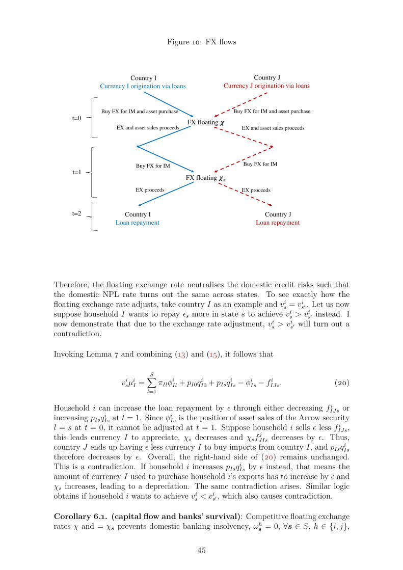
Figure 10: FX flows

Country I Currency I origination via loans

Country JCurrency J origination via loan�

FX floating �

FX floating ��

Country I Loan repayment

Country JLoan repayment

t=0

t=1

Buy FX for IM and asset purchase Buy FX for IM and asset purchase

EX and asset sales proceeds EX and asset sales proceeds

Buy FX for IM Buy FX for IM

EX proceeds EX proceeds

t=2

Therefore, the floating exchange rate neutralises the domestic credit risks such thatthe domestic NPL rate turns out the same across states. To see exactly how thefloating exchange rate adjusts, take country I as an example and vis = vis′ . Let us nowsuppose household I wants to repay εs more in state s to achieve vis > vis′ instead. Inow demonstrate that due to the exchange rate adjustment, vis > vis′ will turn out acontradiction.

Invoking Lemma 7 and combining (13) and (15), it follows that

visµiI =

S∑l=1

πIlφiIl + pI0q

iI0 + pIsq

iIs − φiIs − f iIJs. (20)

Household i can increase the loan repayment by ε through either decreasing f iIJs orincreasing pIsqiIs at t = 1. Since φiIs is the position of asset sales of the Arrow securityl = s at t = 0, it cannot be adjusted at t = 1. Suppose household i sells ε less f iIJs,this leads currency I to appreciate, χs decreases and χsf

jJIs decreases by ε. Thus,

country J ends up having ε less currency I to buy imports from country I, and pIsqiIstherefore decreases by ε. Overall, the right-hand side of (20) remains unchanged.This is a contradiction. If household i increases pIsqiIs by ε instead, that means theamount of currency I used to purchase household i’s exports has to increase by ε andχs increases, leading to a depreciation. The same contradiction arises. Similar logicobtains if household i wants to achieve vis < vis′ , which also causes contradiction.

Corollary 6.1. (capital flow and banks’ survival): Competitive floating exchangerates χ and = χs prevents domestic banking insolvency, ωhs = 0, ∀s ∈ S, h ∈ {i, j},

45

and there is no need for national bailout tax.

Proof. See Appendix D.12.

Corollary 6.2. Under the conditions of Proposition 5, if currency union is the regimea priori, cross-border default due to bankruptcy leniency obviates the need for floatingexchange rates to alleviate domestic banking stress.

Proof. See Appendix D.13.

Corollary 6.1 holds under very general conditions. It states that when there are domes-tic credit risks, floating exchange rates can help absorb the pressure of internationalcapital flow such that domestic banks survive for all states. However, if member coun-tries are in a currency union a priori, cross-country default may obviate such need forfloating exchange rates. In an ideal scenario with zero domestic credit risks, banks getloans repaid in full for all states of nature, and given markets are complete, the roleof floating exchange rate is trivialised (Lemma 5). In other words, if countries do nothave domestic credit risks in all states of nature, even without a fiscal union or defaultin the cross-border capital markets, sharing a common currency brings no particularharm to the health of the banking sector.

As the floating exchange rate neutralised domestic credit risks, one would expect alower transaction wedge in this Regime than in Regime A, because there is no needto level national bailout tax. Lemma 9 refines the FX constraints at t = 0 andunder Lemma 9, Corollaries 6.3-6.6 probe into the BoP dynamics and the welfareimplications for allocations, prices, and risk sharing.

Lemma 9: FX-in-advance binds.

If cov( 1χs, νi2s) > 0 and cov(χs, ν

j2s) > 0, focusing on symmetric equilibrium, rI = rJ ,

then ∆(12) = 0.

Proof. See Appendix D.14.

Corollary 6.3. (Balance of Payments): Under competitive floating exchange ratesand when FX-in-advance binds, current account and capital account exactly balance,CAHs + FAHs = 0, H ∈ {I, J}, s ∈ S.

Proof. See Appendix D.15.

Corollary 6.4. (allocation efficiency within state): Under Lemma 7, optimalallocation efficiency at t = 0 does not obtain due to domestic credit risks and the costof liquidity; optimal allocation within state obtains at t = 1.

U ici

I0

U ici

J0

=U j

cjI0

U j

cjJ0

1(1 + rI)(1 + rJ) ,

U ici

Is

U ici

Js

=U j

cjIs

U j

cjJs

.

46

Proof. See Appendix D.17.

Corollary 6.5. (risk sharing): Under Lemma 7, optimal risk sharing does notobtain due to the borrowing cost which commands the credit risk premium of domesticloans.

U ici

Is

U ici

Is′

=U j

cjIs

U j

cj

Is′

1(1 + rJ)(1 + rI)

,

U ici

Js

U ici

Js′

=U j

cjJs

U j

cj

Js′

1(1 + rJ)(1 + rI)

.

Proof. See Appendix D.18.

Corollary 6.6. (state prices): With national currencies and competitive floatingexchange rate, state prices are affected by the borrow cost and currency appreciationor depreciation.

πIs = γsU ici

Is/pIs

U ici

I0/pI0

= γsU j

cjJs

/pJsχ

U j

cjJ0/pJ0χs(1 + rJ)

,

πJs′ = γs′U ici

Is′/pIs′χs′

U ici

I0/pI0(1 + rI)χ

= γs′U j

cj

Js′/pJs′

U j

cjJ0/pJ0

.

Proof. See Appendix D.19.

5.4 Numerical Analysis

Table (4) displays the numerical result of national currencies and compares it withthose of currency unions. Note that the functional forms and exogenous variablesare the same as in the baseline regime in a currency union. The unique endogenousvariables in the national currency case are the exchange rates at t = 0 and t = 1.

47

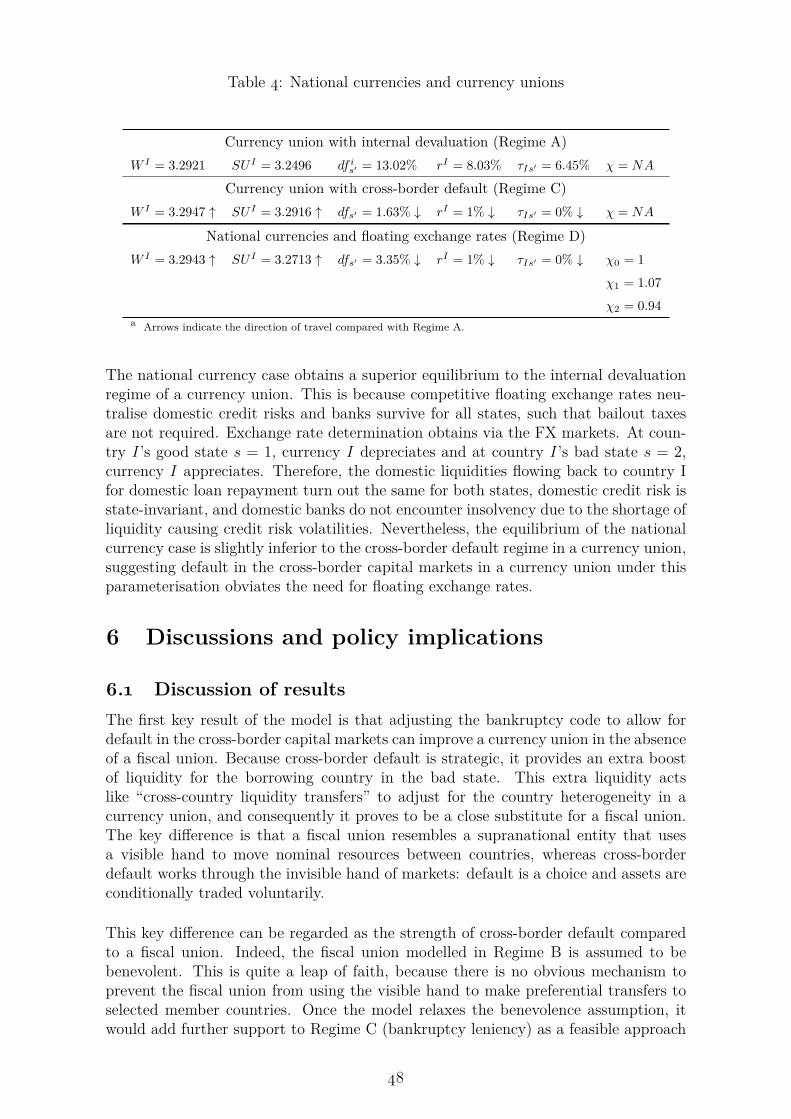
Table 4: National currencies and currency unions

Currency union with internal devaluation (Regime A)W I = 3.2921 SU I = 3.2496 df i

s′ = 13.02% rI = 8.03% τIs′ = 6.45% χ = NA

Currency union with cross-border default (Regime C)W I = 3.2947 ↑ SU I = 3.2916 ↑ dfs′ = 1.63% ↓ rI = 1% ↓ τIs′ = 0% ↓ χ = NA

National currencies and floating exchange rates (Regime D)W I = 3.2943 ↑ SU I = 3.2713 ↑ dfs′ = 3.35% ↓ rI = 1% ↓ τIs′ = 0% ↓ χ0 = 1

χ1 = 1.07

χ2 = 0.94a Arrows indicate the direction of travel compared with Regime A.

The national currency case obtains a superior equilibrium to the internal devaluationregime of a currency union. This is because competitive floating exchange rates neu-tralise domestic credit risks and banks survive for all states, such that bailout taxesare not required. Exchange rate determination obtains via the FX markets. At coun-try I’s good state s = 1, currency I depreciates and at country I’s bad state s = 2,currency I appreciates. Therefore, the domestic liquidities flowing back to country Ifor domestic loan repayment turn out the same for both states, domestic credit risk isstate-invariant, and domestic banks do not encounter insolvency due to the shortage ofliquidity causing credit risk volatilities. Nevertheless, the equilibrium of the nationalcurrency case is slightly inferior to the cross-border default regime in a currency union,suggesting default in the cross-border capital markets in a currency union under thisparameterisation obviates the need for floating exchange rates.

6 Discussions and policy implications

6.1 Discussion of results

The first key result of the model is that adjusting the bankruptcy code to allow fordefault in the cross-border capital markets can improve a currency union in the absenceof a fiscal union. Because cross-border default is strategic, it provides an extra boostof liquidity for the borrowing country in the bad state. This extra liquidity actslike “cross-country liquidity transfers” to adjust for the country heterogeneity in acurrency union, and consequently it proves to be a close substitute for a fiscal union.The key difference is that a fiscal union resembles a supranational entity that usesa visible hand to move nominal resources between countries, whereas cross-borderdefault works through the invisible hand of markets: default is a choice and assets areconditionally traded voluntarily.

This key difference can be regarded as the strength of cross-border default comparedto a fiscal union. Indeed, the fiscal union modelled in Regime B is assumed to bebenevolent. This is quite a leap of faith, because there is no obvious mechanism toprevent the fiscal union from using the visible hand to make preferential transfers toselected member countries. Once the model relaxes the benevolence assumption, itwould add further support to Regime C (bankruptcy leniency) as a feasible approach

48

to sustain currency unions.

However, the limitation of Regime C (bankruptcy leniency) is that it relies on theassumption that the institutional qualities or the economic fundamentals of membercountries in the currency union do not differ significantly. Suppose the two countrieshave divergent economic fundamentals to start with, for example, country J in its goodstate is much poorer than country I in its respective good state. Then in state s′, i.e.country I’s bad state and country J ’s good state, such a lenient union-wide bankruptcycode may encourage country J to even fully default in its good state. In this scenario,capital markets union collapses, impeding international risk sharing and leading towelfare loss. In this case, the within-union standard fails, and there is simply no roomto adjust for the union-wide bankruptcy code. If the model is extended to incorporateproduction and capital accumulation for multi-periods, the issue becomes more acute.Adjusting the bankruptcy code would need to be timely, because a delay would leadcountries to fall out of the within-union standard endogenously due to the persistentinternal devaluation effect. Moreover, even if their fundamentals do not differ toomuch, if country I has a lower institution quality, i.e. its domestic bankruptcy codeλi is much weaker than that of country J , Corollary 3.2 suggests that there simplymay not be any space left to adjust the union-wide bankruptcy code λ, otherwise thefinancial markets would unravel.

The second key result is that adjusting the bankruptcy code in a currency unioncan obviate the need for nominal exchange rates to neutralise domestic credit risks.Strategic default in the capital markets union is essentially a compensation for the lostbenefits of nominal exchange rates. However, assuming away potential costs of nom-inal exchange rates, the conditions for bankruptcy leniency to allow for cross-borderdefault to neutralise domestic credit risks are more exacting than those for nominal ex-change rates. The conditions for the former entail a lenient cross-country bankruptcycode, a sufficiently low cost of liquidity and a sufficiently high number of bad states,but the conditions for the latter are more general. However, nominal exchange ratescould potentially incur (unmodelled) costs, such as competitive devaluation because ofdiscretionary intervention by national governments. Such considerations would rendercross-country default in a currency union a more attractive regime.

Furthermore, this model sets the union-wide bankruptcy code of the capital marketsunion conditional on domestic bankruptcy codes, which are taken as structural parame-ters. In contrast, Franks and Sussman (2005) constructed an endogenous evolutionarytheory of bankruptcy codes, in which bankruptcy codes can emerge either due to free-dom of contracting of market participants or because of state activism in law-making.In this paper, I do not model the endogenous emergence of the bankruptcy codes,but I acknowledge that in practice the softening of the bankruptcy code in the capitalmarkets union could emerge via either market forces or law-making, or a combinationof both.

6.2 Policy implications and implementation

The immediate policy recommendation is that a currency union needs a capital mar-kets union that features a slightly softened bankruptcy environment. Softening thecross-border bankruptcy environment can take measures to encourage more reorgani-

49

sation rather than immediate liquidation of assets when companies become insolvent,to shorten the period of credit market exclusion for the defaulters, or to allow fordebt discharges and adjustments. To increase the space to design such a union-widebankruptcy code to induce benign default in the capital markets union, the domesticbankruptcy code, however, should not be too lenient. Thus, when a fiscal union isabsent in a currency union, member countries should strengthen their domestic insti-tutions by toughening the domestic bankruptcy code for domestic borrowing, and atthe same time mutually agree on a softened union-wide bankruptcy code for cross-country borrowing. An important caveat remains that the union-wide bankruptcycode cannot be too lenient. If it is sufficiently lenient, no country would ever repayin any state, leading to the collapse of the capital markets union and impeding risksharing.

This scope for policy is relevant not just for the Eurozone, but also for China whichhas been experiencing prolonged soaring local government debt. The issue for Chinais more nuanced because the local government debt is largely collateralised by landand real estate. It is further complicated by the Chinese government’s implicit guar-antee. Consequently, the talk of default of the local government financing vehicle inChina has sparked off heated debate among policy makers and academics. This real-world example and the associated macro-financial questions could be modelled in theframework of this paper.

As for the implementation of setting the union-wide bankruptcy code that induces de-fault in the capital markets union, the union-wide bankruptcy code should be commonknowledge to all market participants and should be strictly enforced. In this environ-ment, market participants would know that default in cross-border capital marketsis a possibility and ex ante they know exactly the severity of the default punishmentconditional on the size of default. Accordingly, default risks are priced in when assetsare traded prior to the realisation of uncertainty. For example, suppose the union-widebankruptcy code takes the form of credit exclusion as the default punishment and forsimplicity suppose borrowers are countries in the currency union. Market participantsshould know how many periods the defaulter is to be excluded given the size of de-fault. Once a country announces default, it should be excluded from credit to theextent that market participants have come to expect. This kind of implementation,therefore, ensures orderly default. It is important to note the distinction between thistype of orderly default and the unanticipated default whose risk is not correctly pricedin.

The model is kept stylised such that the results and transmission mechanisms are clear;therefore, the model does not specify the exact form of default punishment. A fully-fledged and more realistic quantitative model could certainly provide further micro-foundation for default punishment, such as credit exclusion or sanctions. Nevertheless,no matter what the exact form of default punishment is, as long as it feeds into themarginal rate of substitution across consumptions, the essence of the current stylisedmodel remains.

50

6.3 Institutional Details

6.3.1 The TARGET2 System

The model abstracted away the national central banks; thus, it is difficult to find anexact mapping between the model and the TARGET2 system, which is the Eurozonepayment system connecting national central banks (NCB)) and the European CentralBank (ECB). However, the two key results of this model can still shed light on theongoing debate on the imbalance of the TARGET2 system (see Sinn 2011; Sinn andWollmershäuser 2012; Whelan 2014).

TARGET is the acronym for Trans-European Automated Real-time Gross Settlement

Express Transfer System. In the TARGET2 system, all Eurosystem banks maintainreserve accounts with their national central banks, which are ultimately connectedby ECB as the lender of last resort. The TARGET2 system equips the nationalcentral banks with some degree of money creation power such that the creation of eurovia ECB becomes less rigid. Therefore, the TARGET2 system allows some nationalcentral banks to hold TARGET2 claims and some other national central banks to holdTARGET2 liabilities.

During the Eurozone Crisis, capital flight from the weak periphery largely took theform of depositors moving deposits from weak banks in the periphery into the strongerbanks in the core. This transfer of funds would have bankrupted many banks in theperiphery, but it was recycled back through the TARGET2 system. In this sense, theTARGET2 system provides some cross-country transfers already, partly resemblingthe fiscal transfers in Regime B (fiscal union) of my model. Therefore, in reality, theTARGET2 system has likely reduced the bailout costs of the Eurozone Crisis anddampened the internal devaluation effect in Regime A of this model.

Nevertheless, the imbalance of the TARGET2 system is not completely the same as thecross-country fiscal transfers in Regime B. This is because the imbalance of TARGET2system takes the form of claims and liabilities. These positions are debt positions thateventually need to be settled, whereas Regime B makes fiscal transfers that are freeand clear of any debt obligation. If the debt positions on the TARGET2 system needto be repaid in full eventually, it would merely imply the delay of national bailoutcosts and internal devaluation. If the debt positions on the TARGET2 system were tocarry priced-in credit risks and allow for default, a similar welfare-improving benefitcould arise as that of Regime C (bankruptcy leniency) in this paper.

6.3.2 Cross-border Insolvency Reforms in Practice

A variety of financial securities are traded in the cross-border capital markets in theEurozone. These financial securities can be sovereign bonds of member countries, cor-porate bonds and equities, or structured products of both the public and private debt.The key result of this paper on softening the bankruptcy code in the cross-border cap-ital markets union is a simplification. The insight is the role of a softened bankruptcyenvironment as a compensation for the removal of flexible nominal exchange rates.

Now let us turn to the practical interpretations of this result in conjunction with theinstitutional details of both the default punishment for sovereign debt and the cross-border insolvency reforms for private debt in the context of the Eurozone. There was

51

a wide misperception of the sovereign debt default risks before the Eurozone Crisis.The misperception was that member countries in the Eurozone simply would notdefault, for example, quoting the Economics Commissioner Joaquin Almunia at thetime: “No, Greece will not default. Please. In the euro area, the default does not exist.”However, the synchronisation of sovereign yields between the core and the peripherybefore the crisis does not mean the sovereign debt of the periphery was default-free.This synchronisation was largely a result of reduction in the inflation premium in theperiphery, and the inflation premium was a proxy for the sovereign’s credit risk profile.The reduction in the inflation premium was a natural result of removing the nominalexchange rates, but it does not imply the underlying credit risks suddenly magicallyvanished.

Therefore, it would be sensible to correct such misperception and to acknowledge andallow for sovereign default in a currency union, particularly when a fiscal union is notpresent. In this paper I only model the aggregate country-level debt and I do notmodel the sovereign debt separately; however, the logic of softening the bankruptcycode extends to the sovereign bond markets. In practice, the bankruptcy code forthe sovereign debt often takes the form of such default punishment as credit marketexclusion. Softening this type of default punishment could mean shorten the periodof credit market exclusion per unit of default. In this scenario, when the marginalcost of default is low enough, countries in the Eurozone can declare default and thepunishment should be strictly enforced. What is crucial is the correct pricing of defaultrisks in the sovereign yields.

As for private debt, a softened bankruptcy code can be a result of contracting or legalreforms. Regarding the latter, there have been practical steps in the European Unioncross-border insolvency reform, albeit not for the specific context of the Eurozone. In2012, the European Commission proposed to recast the 2000 Insolvency Regulationwith the main purpose to help identify the competent jurisdiction and applicable lawinsolvency proceedings. As the 2000 Insolvency Regulation carries legal uncertaintywith some of its key concepts defined in general terms (see Sussman 2006), then the2015 recast regulation provided further clarification on the “centre of main interest”(COMI). More importantly, in 2016, the European Commission proposed to adopt adirective on business restructuring and giving the troubled businesses a second chance,softening the traditionally punitive stance on default.

In spirit, the 2016 directive is similar to Chapter 11 of the US Bankruptcy Code, andit seems broadly consistent with the policy implication of my model. Nevertheless,in practice, the cross-border insolvency reforms in EU or the Eurozone are extremelycomplicated because the national-level bankruptcy codes are very diverse (see Davy-denko and Franks 2008). My model speaks to this issue because my result on softeningthe cross-border bankruptcy code is exactly conditional on national-level bankruptcycodes and takes into consideration of their heterogeneity. Thus, my result does notlead to the conclusion of an unconditional top-down harmonisation.

7 Conclusion

This paper has proposed an international finance model specifically for currency unionsto address the following question: what alternative arrangements can improve the

52

financial stability and viability of currency unions when a fiscal union is absent? Thisquestion is important due to the potential for member countries in a currency union torefuse to establish a fiscal union for political reasons. The model is able to show thatone alternative arrangement is a financial regime that features a softened bankruptcyenvironment in the cross-border capital markets within a currency union.

There are two contributions of this proposed theory. First, the model shows that whendomestic credit risks are present and when there is no fiscal union to make cross-country transfers, endogenous default in the capital markets union within a currencyunion can lead to a Pareto improvement and enhance the viability of a currency union.Second, the model answers the question of why default in the cross-border capitalmarkets is particularly vital for currency unions. That is, under very general conditionscompetitive floating exchange rates are shown to neutralise domestic credit risks andimprove welfare, and sharing a common currency loses such benefits of exchange rates.However, default in the cross-border capital markets under certain conditions recoupsthe lost benefits of exchange rates. Therefore, when countries join a currency unionwith an incomplete fiscal union or banking union, the bankruptcy code needs to adjust.

I acknowledge that the endogenous determination of default punishment and the en-dogenous adoption of currency unions should be the subject of further research. Thebankruptcy code λ is the key parameter of default punishment, and it is essentiallythe price of default. Suppose countries take the price of default as given and “de-mand” default, then the system would need the “supply” of default to endogenise theprice. This sits right at the intersection between law, finance, and political economy.Moreover, this paper takes currency unions as given and the model does not explicitlyexplain why countries choose to adopt a currency union. One possible explanationis that some countries do not have the institutional capacity to implement a credibledomestic bankruptcy code and excessively choose inflation or devaluation as “soft de-fault”. Again, this argument goes back to the first point on endogenising the price ofdefault. Excessive inflation or devaluation incurs the cost of persistent capital outflowand further political costs. Therefore, countries adopt a currency union by giving uptheir monetary autonomy as a self-commitment device.

In conclusion, a broader role of this paper is an initial attempt to bridge the gapbetween the value of money, exchange rate determination and bankruptcy codes ininternational finance. This opens new avenues for the research on the endogenousemergence of international dominant currencies and global financial cycles.

53

References

Acharya, V., Drechsler, I., and Schnabl, P. (2014). A pyrrhic victory? bank bailoutsand sovereign credit risk. The Journal of Finance, 69(6):2689–2739.

Acharya, V. V. and Rajan, R. G. (2013). Sovereign debt, government myopia, andthe financial sector. The Review of Financial Studies, 26(6):1526–1560.

Acharya, V. V. and Steffen, S. (2015). The “greatest” carry trade ever? understandingeurozone bank risks. Journal of Financial Economics, 115(2):215–236.

Adam, K. and Grill, M. (2017). Optimal sovereign default. American Economic

Journal: Macroeconomics, 9(1):128–64.

Adrian, T., Etula, E., and Muir, T. (2014). Financial intermediaries and the cross-section of asset returns. The Journal of Finance, 69(6):2557–2596.

Aguiar, M., Amador, M., Farhi, E., and Gopinath, G. (2015). Coordination and crisisin monetary unions. The Quarterly Journal of Economics, 130(4):1727–1779.

Aguiar, M. and Gopinath, G. (2006). Defaultable debt, interest rates and the currentaccount. Journal of International Economics, 69(1):64–83.

Arellano, C. (2008). Default risk and income fluctuations in emerging economies.American Economic Review, 98(3):690–712.

Arellano, C. and Ramanarayanan, A. (2012). Default and the maturity structure insovereign bonds. Journal of Political Economy, 120(2):187–232.

Asonuma, T. and Trebesch, C. (2016). Sovereign debt restructurings: preemptive orpost-default. Journal of the European Economic Association, 14(1):175–214.

Becker, B. and Ivashina, V. (2017). Financial repression in the european sovereigndebt crisis. Review of Finance, 22(1):83–115.

Bianchi, J. and Bigio, S. (2018). Banks, liquidity management and monetary policy.(under revision for Econometrica).

Bigio, S. and Weill, P.-O. (2016). A theory of bank balance sheets. Working Paper.

Bloise, G., Dréze, J. H., and Polemarchakis, H. M. (2005). Monetary equilibria overan infinite horizon. Economic Theory, 25(1):51–74.

Bloise, G., Polemarchakis, H., and Vailakis, Y. (2017). Sovereign debt and incentivesto default with uninsurable risks. Theoretical Economics, 12(3):1121–1154.

Bloise, G. and Polemarchakis, H. M. (2006). Theory and practice of monetary policy.Economic Theory, 27(1):1–23.

Bolton, P. and Jeanne, O. (2007). Structuring and restructuring sovereign debt: therole of a bankruptcy regime. Journal of Political Economy, 115(6):901–924.

Bolton, P. and Oehmke, M. (2018). Bank resolution and the structure of global banks.The Review of Financial Studies, 32(6):2384–2421.

Bongaerts, D., De Jong, F., and Driessen, J. (2017). An asset pricing approach toliquidity effects in corporate bond markets. The Review of Financial Studies,30(4):1229–1269.

54

Brunnermeier, M. K., Garicano, L., Lane, P. R., Pagano, M., Reis, R., Santos, T.,Thesmar, D., Van Nieuwerburgh, S., and Vayanos, D. (2016). The sovereign-bank diabolic loop and esbies. American Economic Review, 106(5):508–12.

Brunnermeier, M. K. and Reis, R. (2015). A crash course on the euro crisis. PrincetonUniversity and Columbia University manuscript.

Brunnermeier, M. K. and Sannikov, Y. (2016). The i theory of money. NBER WorkingPaper No.22533.

Buiter, W. H. (1999). The fallacy of the fiscal theory of the price level. NBER WorkingPaper No. W7302.

Bulow, J. and Rogoff, K. (1989). Sovereign debt: Is to forgive to forget? American

Economic Review, 79(1):43–50.

Calvo, G. A. (1988). Servicing the public debt: The role of expectations. The American

Economic Review, pages 647–661.

Corsetti, G. and Dedola, L. (2013). The mystery of the printing press: self-fulfillingdebt crises and monetary sovereignty.

Davydenko, S. A. and Franks, J. R. (2008). Do bankruptcy codes matter? a study ofdefaults in france, germany, and the uk. The Journal of Finance, 63(2):565–608.

DeAngelo, H. and Stulz, R. M. (2015). Liquid-claim production, risk management,and bank capital structure: Why high leverage is optimal for banks. Journal of

Financial Economics, 116(2):219–236.

D’Erasmo, P. and Mendoza, E. G. (2016). Distributional incentives in an equilib-rium model of domestic sovereign default. Journal of the European Economic

Association, 14(1):7–44.

Diamond, D. W. and Rajan, R. G. (2001). Liquidity risk, liquidity creation, andfinancial fragility: A theory of banking. Journal of political Economy, 109(2):287–327.

Donaldson, J. R., Piacentino, G., and Thakor, A. (2018). Warehouse banking. Journalof Financial Economics, 129(2):250 – 267.

Drèze, J. H. and Polemarchakis, H. M. (2001). Monetary equilibria. In Economics

Essays, pages 83–108. Springer.

Dubey, P. and Geanakoplos, J. (1992). The value of money in a finite horizon economy:a role for banks. Cowles Foundation Paper 901.

Dubey, P. and Geanakoplos, J. (2003a). Inside and outside fiat money, gains to trade,and is-lm. Economic Theory, 21(2-3):347–397.

Dubey, P. and Geanakoplos, J. (2003b). Monetary equilibrium with missing markets.Journal of Mathematical Economics, 39(5-6):585–618.

Dubey, P. and Geanakoplos, J. (2006). Determinacy with nominal assets and outsidemoney. Economic theory, 27(1):79–106.

Dubey, P., Geanakoplos, J., and Shubik, M. (2005). Default and punishment in generalequilibrium. Econometrica, 73(1):1–37.

55

Dubey, P. and Shubik, M. (1977). A theory of money and financial institutions. part36. the money rate of interest (a multiperiod nonatomic trading and productioneconomy with outside money, inside money and optimal bankruptcy rules). Tech-nical report, YALE UNIV NEW HAVEN CONN COWLES FOUNDATION FORRESEARCH IN ECONOMICS.

Eaton, J. and Gersovitz, M. (1981). Debt with potential repudiation: Theoretical andempirical analysis. The Review of Economic Studies, 48(2):289–309.

Espinoza, R. A., Goodhart, C. A., and Tsomocos, D. P. (2009). State prices, liquidity,and default. Economic Theory, 39(2):177–194.

Farhi, E. and Tirole, J. (2017). Deadly embrace: Sovereign and financial balancesheets doom loops. The Review of Economic Studies, 85(3):1781–1823.

Farhi, E. and Werning, I. (2017). Fiscal unions. American Economic Review,107(12):3788–3834.

Faure, S. A. and Gersbach, H. (2017). Loanable funds vs money creation in banking:a benchmark result. CFS Working Paper Series, No. 587.

Ferrero, A. (2009). Fiscal and monetary rules for a currency union. Journal of

International Economics, 77(1):1–10.

Fisher, I. (1933). The debt-deflation theory of great depressions. Econometrica,1(4):337–357.

Foarta, D. (2018). The limits to partial banking unions: A political economy approach.American Economic Review, 108(4-5):1187–1213.

Franks, J. and Sussman, O. (2005). Financial innovations and corporate bankruptcy.Journal of Financial Intermediation, 14(3):283–317.

Friedman, M. (1997). The euro: monetary unity to political disunity. Project Syndi-

cate, 28.

Fuchs, W. and Lippi, F. (2006). Monetary union with voluntary participation. The

Review of Economic Studies, 73(2):437–457.

Gabrieli, S. and Labonne, C. (2018). Bad sovereign or bad balance sheets? eurointerbank market fragmentation and monetary policy, 2011-2015.

Gali, J. and Monacelli, T. (2005). Monetary policy and exchange rate volatility in asmall open economy. The Review of Economic Studies, 72(3):707–734.

Gali, J. and Monacelli, T. (2008). Optimal monetary and fiscal policy in a currencyunion. Journal of International economics, 76(1):116–132.

Geanakoplos, J. and Tsomocos, D. P. (2002). International finance in general equilib-rium. Research in Economics, 56(1):85–142.

Gennaioli, N., Martin, A., and Rossi, S. (2014). Sovereign default, domestic banks,and financial institutions. The Journal of Finance, 69(2):819–866.

Goodhart, C. and Jensen, M. (2015). Currency school versus banking school: anongoing confrontation. Economic Thought, 4(2):20–31.

Goodhart, C. A. (1997). Two concepts of money, and the future of europe. Optimum

Currency Areas-New Analytical and Policy Developments, pages 89–96.

56

Goodhart, C. A. (1998). The two concepts of money: implications for the analysis ofoptimal currency areas. European Journal of Political Economy, 14(3):407–432.

Goodhart, C. A., Kashyap, A. K., Tsomocos, D. P., and Vardoulakis, A. P. (2012).Financial regulation in general equilibrium. Technical report, National Bureau ofEconomic Research.

Goodhart, C. A., Kashyap, A. K., Tsomocos, D. P., Vardoulakis, A. P., et al. (2013).An integrated framework for analyzing multiple financial regulations. Interna-

tional Journal of Central Banking, 9(1):109–143.

Goodhart, C. A., Peiris, M. U., and Tsomocos, D. P. (2018). Debt, recovery rates andthe greek dilemma. Journal of Financial Stability, 36:265–278.

Goodhart, C. A., Sunirand, P., and Tsomocos, D. P. (2006). A model to analysefinancial fragility. Economic Theory, 27(1):107–142.

Gordon, G. and Guerron-Quintana, P. (2018). A quantitative theory of hard and softsovereign defaults.

Gorton, G. and Pennacchi, G. (1990). Financial intermediaries and liquidity creation.The Journal of Finance, 45(1):49–71.

Graeber, D. (2012). Debt: The First 5000 Years. Penguin UK.

Grandmont, J.-M. and Younes, Y. (1972). On the role of money and the existence ofa monetary equilibrium. The Review of Economic Studies, 39(3):355–372.

Grandmont, J.-M. and Younes, Y. (1973). On the efficiency of a monetary equilibrium.The Review of Economic Studies, 40(2):149–165.

Gu, C., Mattesini, F., and Wright, R. (2016). Money and credit redux. Econometrica,84(1):1–32.

Guembel, A. and Sussman, O. (2004). Optimal exchange rates: a market microstruc-ture approach. Journal of the European Economic Association, 2(6):1242–1274.

Guembel, A. and Sussman, O. (2009). Sovereign debt without default penalties. TheReview of Economic Studies, 76(4):1297–1320.

Gurley, J. G. and Shaw, E. S. (1960). Money in a theory of finance. Washington, DC:Brookings Institution.

Hahn, A. (1920). Volkswirtschaftliche theorie des bankkredits. Tübingen: J.C.B.Mohr.

Hart, O. and Zingales, L. (2014). Banks are where the liquidity is. Technical report,National Bureau of Economic Research.

Hawtrey, R. G. (1923). Currency and Credit. Longmans, Green.

He, Z., Kelly, B., and Manela, A. (2017). Intermediary asset pricing: New evidencefrom many asset classes. Journal of Financial Economics, 126(1):1–35.

He, Z. and Krishnamurthy, A. (2013). Intermediary asset pricing. American Economic

Review, 103(2):732–70.

Huang, L. and Winton, A. (2016). Soft collateral, bank lending, and the optimal creditrating system. Bank Lending, and the Optimal Credit Rating System (November

8, 2016).

57

J Caballero, R. and Farhi, E. (2017). The safety trap. The Review of Economic

Studies, 85(1):223–274.

Kehoe, P. J. and Pastorino, E. (2017). Fiscal unions redux. Economic Theory,64(4):741–776.

Kenen, P. (1969). The theory of optimum currency areas: an eclectic view. Monetary

problems of the international economy, 45(3):41–60.

Keynes, J. M. (1931). The consequences to the banks of the collapse of money values.In Essays in Persuasion, pages 150–158. Springer 2010.

Kiyotaki, N. and Moore, J. (2018a). Inside money and liquidity. Working paper.

Kiyotaki, N. and Moore, J. (2018b). Liquidity, business cycles, and monetary policy.Forthcoming in Journal of Political Economy.

Kondor, P. and Vayanos, D. (2019). Liquidity risk and the dynamics of arbitragecapital. The Journal of Finance, 74(3):1139–1173.

Kumhof, M. and Wang, X. (2018). Banks, money and the zero lower bound on depositrates. Bank of England Staff Working Papers No. 752.

Lane, P. R. (2012). The european sovereign debt crisis. Journal of Economic Perspec-

tives, 26(3):49–68.

Lin, L., Tsomocos, D. P., and Vardoulakis, A. P. (2016). On default and uniquenessof monetary equilibria. Economic Theory, 62(1-2):245–264.

Lucas Jr, R. E. and Stokey, N. (1987). Money and interest in a cash-in-advanceeconomy. Econometrica, 55(3):491–513.

Macleod, H. D. (1866). The Theory and Practice of Banking: with the elementary

principles of Currency, Prices, Credit, and Exchanges, volume 1.

Manova, K. (2012). Credit constraints, heterogeneous firms, and international trade.Review of Economic Studies, 80(2):711–744.

Martinez, J., Philippon, T., and Sihvonen, M. (2019). Does a currency union need acapital market union? risk sharing via banks and markets. NBER Working Paper26026.

McKinnon, R. I. (1963). Optimum currency areas. The American Economic Review,53(4):717–725.

McMahon, M., Peiris, M. U., and Polemarchakis, H. (2018). Perils of unconventionalmonetary policy. Journal of Economic Dynamics and Control, 93:92–114.

Mendoza, E. G. and Yue, V. Z. (2012). A general equilibrium model of sovereigndefault and business cycles. The Quarterly Journal of Economics, 127(2):889–946.

Minsky, H. P. (1977). The financial instability hypothesis: an interpretation of keynesand an alternative to ‘standard’ theory. Nebraska Journal of Economics and

Business, 16(1):5–16.

Mitman, K. (2016). Macroeconomic effects of bankruptcy and foreclosure policies.American Economic Review, 106(8):2219–55.

58

Mundell, R. A. (1961). A theory of optimum currency areas. The American Economic

Review, 51(4):657–665.

Na, S., Schmitt-Grohé, S., Uribe, M., and Yue, V. (2018). The twin ds: Optimaldefault and devaluation. American Economic Review, 108(7):1773–1819.

Neumeyer, P. A. (1998). Currencies and the allocation of risk: the welfare effects of amonetary union. American Economic Review, pages 246–259.

Obstfeld, M. and Rogoff, K. (2000). New directions for stochastic open economymodels. Journal of International Economics, 50(1):117–153.

Ongena, S., Popov, A. A., and Van Horen, N. (2018). The invisible hand of thegovernment:’moral suasion’during the european sovereign debt crisis.

Peiris, M. U. and Tsomocos, D. P. (2015). International monetary equilibrium withdefault. Journal of Mathematical Economics, 56:47–57.

Perotti, E. and Soons, O. (2019). The political economy of a diverse monetary union.Working Paper.

Piazzesi, M. and Schneider, M. (2018). Payments, credit and asset prices. BIS WorkingPapers, No. 737.

Reis, R. (2013). The mystique surrounding the central bank’s balance sheet, appliedto the european crisis. American Economic Review, 103(3):135–40.

Sargent, T. J. (2012). Nobel lecture: United states then, europe now. Journal of

Political Economy, 120(1):1–40.

Schumpeter, J. A. (1954). History of Economic Analysis. New York: Oxford UniversityPress.

Shapley, L. and Shubik, M. (1977). Trade using one commodity as a means of payment.Journal of political economy, 85(5):937–968.

Shubik, M. (1999). The Theory of Money and Financial Institutions, volume 1. Cam-bridge, MA: MIT Press.

Shubik, M. and Tsomocos, D. P. (1992). A strategic market game with a mutualbank with fractional reserves and redemption in gold. Journal of Economics,55(2):123–150.

Shubik, M. and Wilson, C. (1977). The optimal bankruptcy rule in a trading economyusing fiat money. Journal of economics, 37(3):337–354.

Sims, C. A. (1994). A simple model for study of the determination of the price leveland the interaction of monetary and fiscal policy. Economic theory, 4(3):381–399.

Sinn, H.-W. (2011). The ecb’s secret bailout strategy, project syndicate, 29. april 2011.

Sinn, H.-W. and Wollmershäuser, T. (2012). Target loans, current account balancesand capital flows: the ecb’s rescue facility. International Tax and Public Finance,19(4):468–508.

Stein, J. C. (2012). Monetary policy as financial stability regulation. The Quarterly

Journal of Economics, 127(1):57–95.

Sussman, O. (2006). The economics of the eu’s corporate-insolvency law and the questfor harmonisation by market forces. Unpublished working paper.

59

Tobin, J. (1963). Commercial banks as creators of ’money’. Technical report, CowlesFoundation for Research in Economics, Yale University.

Trebesch, C. and Zabel, M. (2017). The output costs of hard and soft sovereign default.European Economic Review, 92:416–432.

Tsomocos, D. P. (2003). Equilibrium analysis, banking and financial instability. Jour-nal of Mathematical Economics, 39(5-6):619–655.

Tsomocos, D. P. (2008). Generic determinacy and money non-neutrality of interna-tional monetary equilibria. Journal of Mathematical Economics, 44(7-8):866–887.

Tsomocos, D. P. and Wang, X. (2019). Financial stability, endogenous liquidity, andmonetary policy transmission in the interest rate lower bound. Working Paper.

Uhlig, H. (2014). Sovereign default risk and banks in a monetary union. German

Economic Review, 15(1):23–41.

Uribe, M. (2006). A fiscal theory of sovereign risk. Journal of Monetary Economics,53(8):1857–1875.

Whelan, K. (2014). Target2 and central bank balance sheets. Economic Policy,29(77):79–137.

White, M. J. (1983). Bankruptcy costs and the new bankruptcy code. The Journal

of Finance, 38(2):477–488.

Wicksell, K. (1906). Lectures on political economy vol. ii money.

Woodford, M. (2010). Financial intermediation and macroeconomic analysis. Journalof Economic Perspectives, 24(4):21–44.

Zame, W. R. (1993). Efficiency and the role of default when security markets areincomplete. The American Economic Review, pages 1142–1164.

60

Appendices

A Currency Union - country J

A.1 Country J

Household j

Household j consumes both the domestic goods and foreign goods at t = 0 and t = 1and suffers a non-pecuniary penalty from default. Household j’s maximisation problemis outlined as follows:

Max︸ ︷︷ ︸µj

J ,θj ,φj ,cj

J ,cjI ,q

jJ ,b

jI ,v

j ,Dj

E0

{U j(cjJ0, c

jI0, c

jJs, c

jIs

)− λj[djs]+ − λ[f js ]+

},

where λj[djs]+ = λjmax[(1 − vjs)µjJ/ps, 0] is the non-pecuniary cost of domestic loan

default, and λ[f js ]+ = λmax[(φjs−Djs)/ps, 0] is the non-pecuniary cost of cross-country

default.

Subject to

bjI0 +S∑l=1

πlθjl ≤

µjJ1 + rJ

+mj, (21)

bjIs(1 + τJs) + (Djs −Ksθ

js) + φjsτJs ≤ ∆(21) +

S∑l=1

πlφjl + pI0q

iI0 + pJsq

jJs + δjs, (22)

vjsµjJ ≤ ∆(22)s. (23)

And for s∗ ∈ S∗, the feasibility constraints are satisfied, i.e. cjJs∗ ≤ ejJs∗ − qjJs∗ and

cjIs∗ ≤bj

Is∗pIs∗

. At t = 0, household j borrows from the domestic commercial bank j

to get money to buy nominal Arrow securities and imports. Household j also getsmonetary income by selling nominal Arrow securities and exports that gets carriedover to the next period. At t = 1, household j sells exports and uses existing moneyto purchase imports and deliver (net) asset payoffs subject to domestic tax levy. Att = 2, household j uses unused money to settle outstanding loans and chooses howmuch to repay or default.

Domestic Commercial Bank j

Bank j extends loans and provides liquidity for household j. To ensure the liquiditybank j provides has a one-to-one convertibility with the common currency the union-wide central bank issues, bank j needs to borrow interbank loans from the union-widecentral bank. Similar to bank i, bank j’s maximisation problem is outline as follows,

61

Max︸ ︷︷ ︸µj

CB ,µjJ ,L

j ,ωj

S∑s=1

zsωjs,

subject to

Lj ≤ µjCB1 + ρ

, (24)

µjJ1 + rJ

≤ Lj, (25)

ωjs = ∆(24) + ∆(25) +Rjsµ

jJ − µ

jCB. (26)

At the beginning of t = 0, bank j borrows from the union-wide central bank andobtain fiat money in the common currency, ready to be extended as interbank liquidityLj. Then bank j extends loans to the domestic households but has to ensure theliquidity bank j provides against the bank loans has a one-to-one convertibility withthe fiat money issued by the central bank. At t = 2, bank j uses the households’ loanrepayments to pay back the interbank loans to the union-wide central bank.

National Government j

National government j collects taxes from the domestic household based on importexpenditures and cross-country borrowing to build a state-contingent bailout fund ofTJs.

TJs = pIscjIsτJs + φjsτJs.

National government j uses the bailout funds to rescue the national commercial bankwhenever the bank’s nominal profits would drop to negative. This is to ensure ωjs +TJs = 0 at the bad state.

62

B Regime D - Country J

B.1 Structure and Flows

Figure 11: Nominal flows of the economy

National central bank �

Domestic commercial bank �

Country � Country �

Domestic commercial bank �

Households � Households �

Interbank loans Currency � Interbank loansCurrency �

Loans Liquidity Liquidity LoansAsset Markets �

Goods markets

National central bank �

FX markets

Asset Markets �

B.2 Regime D Timeline

Figure 12: Timeline

Loan markets open, money provided against bank credit,FX market opens

State of nature unfolds

FX market opens again,Goods market trade and asset market delivery

t=0 t=1

Goods and asset market receipts to carry over Loan settlement

subject to default Goods and asset market purchases

t=2

63

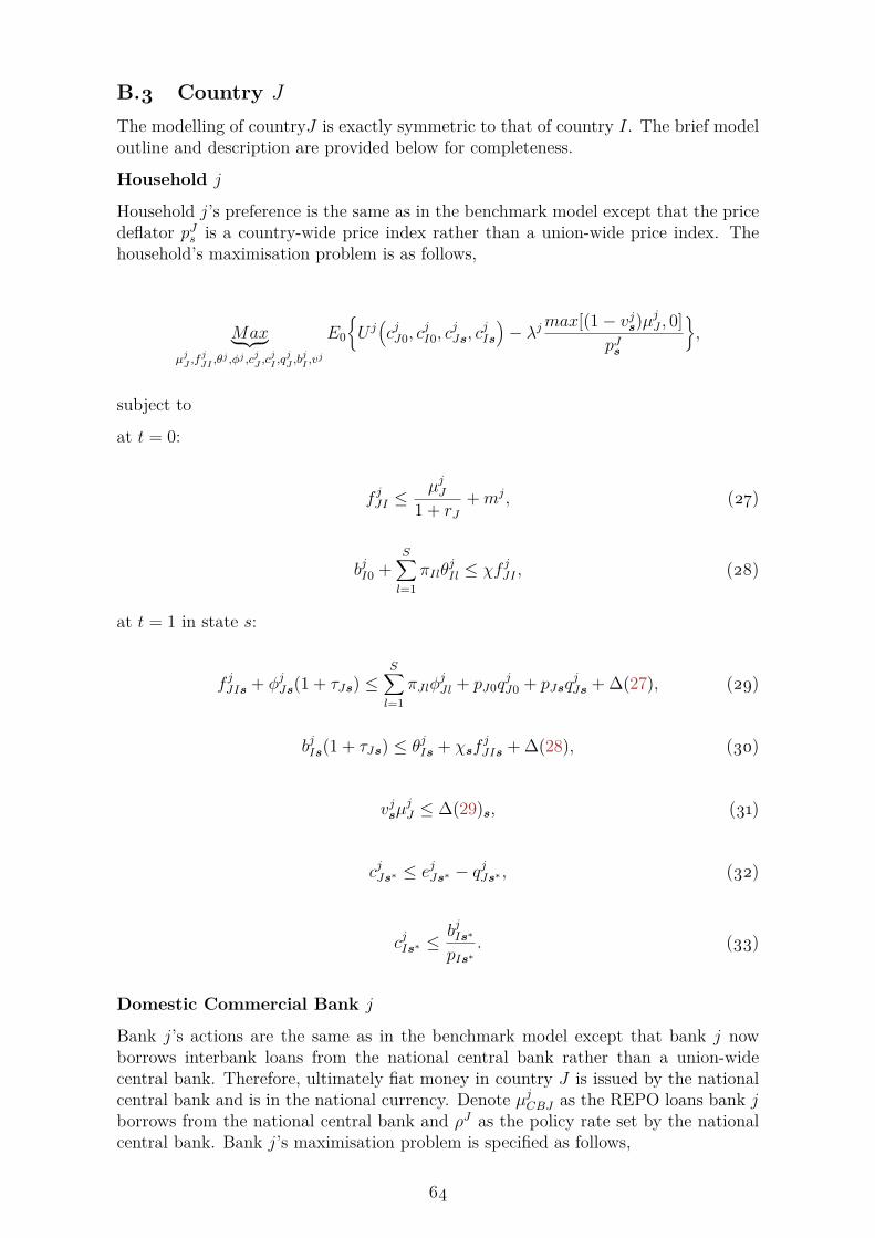
B.3 Country J

The modelling of countryJ is exactly symmetric to that of country I. The brief modeloutline and description are provided below for completeness.

Household j

Household j’s preference is the same as in the benchmark model except that the pricedeflator pJs is a country-wide price index rather than a union-wide price index. Thehousehold’s maximisation problem is as follows,

Max︸ ︷︷ ︸µj

J ,fjJI ,θ

j ,φj ,cjJ ,c

jI ,q

jJ ,b

jI ,v

j

E0

{U j(cjJ0, c

jI0, c

jJs, c

jIs

)− λjmax[(1− vjs)µ

jJ , 0]

pJs

},

subject to

at t = 0:

f jJI ≤µjJ

1 + rJ+mj, (27)

bjI0 +S∑l=1

πIlθjIl ≤ χf jJI , (28)

at t = 1 in state s:

f jJIs + φjJs(1 + τJs) ≤S∑l=1

πJlφjJl + pJ0q

jJ0 + pJsq

jJs + ∆(27), (29)

bjIs(1 + τJs) ≤ θjIs + χsfjJIs + ∆(28), (30)

vjsµjJ ≤ ∆(29)s, (31)

cjJs∗ ≤ ejJs∗ − qjJs∗ , (32)

cjIs∗ ≤bjIs∗

pIs∗. (33)

Domestic Commercial Bank j

Bank j’s actions are the same as in the benchmark model except that bank j nowborrows interbank loans from the national central bank rather than a union-widecentral bank. Therefore, ultimately fiat money in country J is issued by the nationalcentral bank and is in the national currency. Denote µjCBJ as the REPO loans bank jborrows from the national central bank and ρJ as the policy rate set by the nationalcentral bank. Bank j’s maximisation problem is specified as follows,

64

Max︸ ︷︷ ︸µj

CBJ ,µjJ ,L

j ,ωj

S∑s

zsωjs,

subject to

Lj ≤ µjCBJ1 + ρJ

, (34)

µjJ1 + rJ

≤ Lj, (35)

ωjs = ∆(34) + ∆(35) +Rjsµ

jJs − µ

jCBJ . (36)

National Government j

National government j collects taxes from domestic households to build a state-contingent bailout fund of TJs.

TJs = pIscjIsτJs + φjsτJs. (37)

National government j uses the bailout funds to rescue the domestic commercial bankwhenever the bank’s nominal profits would drop to negative, i.e. the bank fails. Inshort, at the bad state the national government makes a state-contingent transfer toensure ωjs + TJs = 0.

National Central Bank j

The national central bank lends REPO loans µJCBJ to the domestic commercial bankand provides fiat money in the national currency. The national central bank sets theREPO loan rate ρJ .

C Equilibrium and Regime Characterisation

C.1 Proof of Lemma 1.

Proof. First, I identify the condition for household i’s liquidity-in-advance constraintto bind. Suppose rI > 0 and suppose further household i does not spend on all themoney at hand, i.e. ∆(1) > 0. The household can borrow ε less loan, but it only leadsto ε/(1 + rI) reduction on the money at hand from (1).

Moreover, from (3), the reduction of loan needing to repay is visε, and the pecuniarybenefit due to the reduction of default cost amounts to (1− vis)ε. Thus, there is extramoney (vis − 1/(1 + rI) + 1 − vis)/ε = rIε/(1 + rI) at t = 2. Household i can eitheruse this extra money to consume more or increase loan repayment, and both lead towelfare improvement. This is a contradiction; hence, ∆(1) = 0.

Second, I prove the binding condition for bank i’s liquidity-in-advance constraint.Suppose bank i does not extend all the money at hand as interbank liquidity to

65

household i, i.e. ∆(4) > 0. Bank i can borrow ε less interbank loan, but it only leadsto ε/(1 + ρ) reduction on the money at hand in (6). The reduction of loan needing torepay is ε, which means there is an extra money of ρε/(1 + ρ) in (6) that adds to banki’s cash flow, increasing its utility. This is a contradiction. Hence, ∆(4) = 0. �

C.2 Proof of Lemma 2

Proof. Suppose ∆(5) > 0, bank i can reduce the interbank liquidity Li by ε, given (4)binds, it means bank i borrows (1 + ρ)ε less interbank loans. From (6), the money athand is reduced by ε, but the interbank loan needing to repay is reduced by (1 + ρ)ε.This means there is an extra money of ρε that adds to bank i’s cash flow at t = 2,increasing its utility. This is a contradiction. Hence, ∆(5) = 0. �

C.3 Proof of Lemma 3.

Proof. Suppose ∆s(3) > 0, then household i can either increase repayment rate vis orborrow ε more at the interest rate of rI . If household i increases vis, it leads to animmediate increase in utility because the cost of default decreases This improvementof welfare means a contradiction. If household i borrows ε more, then household ihas an extra money of ε/(1 + rI) and uses it to buy more imports or sell less exports,leaving all other actions unchanged, without violating the inequality (3), because thehousehold has enough money at hand to repay the extra loan. The improvement ofwelfare means a contradiction.

Similarly contradiction arises if ∆s(6) > 0. Therefore, ∆s(3) = 0 and ∆s(6) = 0. �

C.4 Proof of Lemma 4.

Proof. Suppose φis > 0, θis′ > 0. From household i’s perspective, the FOC for φisleads to πs

U i

ciI0

pI0= (1 + τIs)γsηI1s. FOC for θis′ leads to πs′

U i

ciJ0

pJ0= γs′η

i1s′ . Suppose

ηi1s = ηi1s′ , and also the FOCs for ciI0, ciJ0, and µiI lead toU i

ciJ0

pJ0= (1 + rI)

U i

ciI0

pI0, it follows

πs

(1+τIs)γs= πs′ (1+rI)

γs′. Hence,

πsγs′ > πs′γs. (38)

On the other hand, from household j’s perspective, household j’s FOC for θjs leads to

πs

Uj

cjI0

pI0= γsη

j1s, FOC for φjs′ gives πs′

Uj

cjJ0

pJ0= γs′(1 + τJs′)ηj1s′ . Given ηj1s = ηj1s′ , and also

the FOCs for cjJ0, cjI0, µ

jJ lead to

Uj

cjI0

pI0= (1+rJ)

Uj

cjJ0

pJ0, it follows that πs(1+rJ )

γs= πs′

(1+τJs′ )γs′.

Hence,

π1γ2 < π2γ1. (39)

We can see that (39) contradicts (38).

Suppose θis > 0, φis′ > 0, by the same logic, a contradiction also arises. Therefore, it isnot possible that ηi1s = ηi1s′ and η

j1s = ηj1s′ . �

66

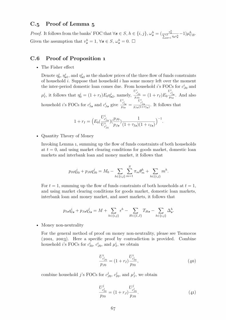
C.5 Proof of Lemma 5

Proof. It follows from the banks’ FOC that ∀s ∈ S, h ∈ {i, j}, ωhs = ( vhs∑S

s=1 ηsvhs

−1)µhCB.Given the assumption that vhs = 1, ∀s ∈ S, ωhs = 0. �

C.6 Proof of Proposition 1

• The Fisher effect

Denote ηi0, ηis1, and ηis2 as the shadow prices of the three flow of funds constraintsof household i. Suppose that household i has some money left over the momentthe inter-period domestic loan comes due. From household i’s FOCs for ciJ0 and

µiI , it follows that ηi0 = (1 + rI)E0ηis2, namely,

U i

ciJ0

pJ0= (1 + rI)E0

U i

ciIs

pIs. And also

household i’s FOCs for ciIs and ciJs giveU i

ciIs

pIs=

U i

ciJs

pJs(1+τIs) . It follows that

1 + rI =(E0(

U ici

Js

U ici

J0

)(pJ0

pJs) 1(1 + τIs)(1 + ιIs)

)−1.

• Quantity Theory of Money

Invoking Lemma 1, summing up the flow of funds constraints of both householdsat t = 0, and using market clearing conditions for goods market, domestic loanmarkets and interbank loan and money market, it follows that

pI0qiI0 + pJ0q

jJ0 = M0 −

∑h∈{i,j}

S∑m=1

πmθhm +

∑h∈{i,j}

mh.

For t = 1, summing up the flow of funds constraints of both households at t = 1,and using market clearing conditions for goods market, domestic loan markets,interbank loan and money market, and asset markets, it follows that

pIsqiIs + pJsq

jJs = M +

∑h∈{i,j}

εh −∑

H∈{I,J}THs −

∑h∈{i,j}

∆hs.

• Money non-neutrality

For the general method of proof on money non-neutrality, please see Tsomocos(2001, 2003). Here a specific proof by contradiction is provided. Combinehousehold i’s FOCs for ciI0, ciJ0, and µiI , we obtain

U ici

J0

pJ0= (1 + rI)

U ici

I0

pI0, (40)

combine household j’s FOCs for cjJ0, cjI0, and µ

jJ , we obtain

U j

cjI0

pI0= (1 + rJ)

U j

cjJ0

pJ0. (41)

67

Suppose the union-wide central bank increases the interbank rate ρ. Supposeconsumption and default remain unchanged. Based on banks’ FOCs that 1+rI =

1+ρ∑S

s=1 zsvis

and 1+rJ = 1+ρ∑S

s=1 zsvjs

, we can see that rI and rJ both increase. Eq(40)implies pI0

pJ0has to increase, whereas Eq(41) implies that pJ0

pI0has to increase. This

is a contradiction. �

C.7 Proof of Corollary 1.1

Proof. Let zs be the risk-neutral probabilities ∀s ∈ S. Bank i’s FOC has 1 + rI =1+ρ∑S

s=1 zsvis

, ωis = visµiI−µiCB = ( vi

s∑S

s=1 zsvis

−1)µiCB. Given the assumption vis >∑Ss=1 zsv

is,

and vis′ <∑S

s=1 zsvis, then ωis > 0, and ωis′ < 0. Similarly, for bank j, ωjs′ > 0 and

ωjs < 0.

At state s, the union-wide central bank’s profits ωCBs = µiCB −µi

CB

1+ρ + vjsµjs−

µjCB

1+ρ + T js .

Rearranging the algebra and plugging in the market clearing condition for interbankloans and money, as well as bank j’s FOCs,

ωCBs =µiCB −µiCB1 + ρ

+ vjsµjJ −

µjCB1 + ρ

+ T js

=µiCB −µiCB1 + ρ

+ vjsµjJ −

1 + ρ

1 + rJµjJ + 1 + ρ

1 + rJµjJ −

µjCB1 + ρ

+ T js

= ρ

1 + ρ(µiCB + µjCB) + (vjs −

(1 + ρ)∑Ss=1 zsv

js

1 + ρ)µjJ + T js

= ρ

1 + ρ(µiCB + µjCB) + (vjs −

(1 + ρ)∑Ss=1 zsv

js

1 + ρ) (1 + ρ)∑S

s=1 zsvjs

µjCB1 + ρ

+ T js

=ρM + ( vjs∑Ss=1 zsv

js

− 1)µjCB + T js ,

Moreover, via the flow of funds and budget constraints of the households and com-mercial banks, total outside money that flows into the union-wide central bank equals∑h∈{i,j}m

h − ωis. Thus,

ρM + ( vjs∑Ss=1 zsv

js

− 1)µjCB + T js =∑

h∈{i,j}mh − ωis.

Similar proof follows for state s′,

ρM + ( vis′∑Ss=1 zsv

is

− 1)µiCB + T is′ =∑

h∈{i,j}mh − ωjs′ .

�

68

C.8 Proof of Proposition 2

Proof. At country I’s bad state s′ when credit risks are present, suppose λ > λi, itmeans the marginal cost of default on financial securities is larger than the marginalcost of default on domestic loans. At the bad state s′, household i’s FOC for vis′ givesλi

ps′=

U i

ciIs′

pIs′, it follows that

λ

ps′>U ici

Is′

pIs′. (42)

The left-hand side of (42) is the marginal cost of default on financial securities andthe right-hand side of (42) is the marginal benefit. Since the marginal cost of defaulton financial securities is larger than the marginal benefit, household i fully delivers oncross-country borrowing, i.e. Di

s′ = φis′ .

At the good state household i’s FOC for vis gives λi

ps≥

U i

ciIs

pIs. Since λ > λi, it follows

that λps>

U i

ciIs

pIs. Hence, Di

s = φis.

Overall, ∀s ∈ S, Dis = φis.

Now suppose the cross-country bankruptcy code is more lenient, i.e. λ < λi. It meansthe marginal cost of default on financial securities is smaller than the marginal cost of

default on domestic loans. At the bad state, λ ≤U i

ciIs′

pIs′, and λi

ps′≥

U i

ciIs′

pIs′. It is less costly

to default on financial securities, so household would default on financial securitiesfirst instead of domestic loans, i.e. Di

s′ < φis′ .

At the good state household i’s FOC for vis gives λi

ps′≥

U i

ciIs′

pIs′, since λ < λi, the

relationship between λps′

andU i

ciIs′

pIs′is ambiguous. The marginal cost of default on

financial securities can be larger than, or equal to, or smaller than the marginal benefit.Therefore, Di

s ≤ φis.

Overall, ∀s ∈ S, Dis ≤ φis. The same logic follows for the case of country J . �

D Equilibrium Analysis

D.1 Proof of Proposition 3

Proof. Since λ̄p2

= ηi11, a2λ̄p2

= ηi22 holds. Given ηj12 < λp2

and a2λ < a2λ̄ < λi,then ηj12 <

λp2< ηi12. These conditions are the on-the-verge conditions between the

households’ marginal benefit of default and their marginal cost of default on Arrowsecurities. Thus, if holding short positions, household i defaults on Arrow securityl = 2 fully while household j fully delivers the payoff of Arrow security l = 2.

Due to risk-aversion, it is straightforward to see that household i buys Arrow security

69

l = 2 because ei1 > ei2, ηi11 < ηi12, and household j sells Arrow security l = 2 becauseej1 < ej2, ηj11 > ηj12. However, to see why household i also sells Arrow security l = s′ atthe same time whenever

(K2 − π2

(vi2(1 + rI) − 1

))/pI2 > π2r

l/pI1 holds, I show viaproof by contradiction.

Suppose φi2 = 0 is the equilibrium outcome. Suppose now household i sells ε amountof Arrow security l = 2. According to the market clearing condition of Asset markets,household i would need to buy ε amount of Arrow security l = 2. This means householdi needs to borrow π2ε more money at t = 0 while needing to pay back π2εv

i2(1 + rI) at

state 2, so the extra monetary cost is π2ε(vi2(1+ rI)−1

). However, because household

i can default fully on the ε amount of Arrow security sold, the extra money inflow dueto default amounts to K2ε, where K2 = 1 − ε∑

h∈i,jφh

2. Thus, the total money inflow

K2ε−π2ε(vi2(1+rI)−1

)is positive. For the good state 1, ηi21 <

λi

p1holds, vi1 = 1, so the

extra monetary cost is π2εrl. If(K2 − π2

(vi2(1 + rI)− 1

))/pI2 > π2r

l/pI1 holds, then

∇U i(·)(K2ε−π2ε(vi2(1+rI)−1

)) > ∇U i(·)(π2εr

l) holds, leading to an overall increasein household i’s expected utility. This is inconsistent with φi2 = 0 as an equilibriumoutcome. �

D.2 First-order conditions of Currency Unions

D.2.1 FOCs of Regimes A & B

:

U ici

J0

pJ0= (1 + rI)E0

U ici

Is

pIs, (43)

U ici

I0

pI0= E0

U ici

Js

pJs(1 + τIs), (44)

U j

cjI0

pI0= (1 + rJ)E0

U j

cjJs

pJs, (45)

U j

cjJ0

pJ0= E0

U j

cjIs

pIs(1 + τJs), (46)

1 + rI = 1 + ρ∑Ss=1 zsv

is

, (47)

1 + rJ = 1 + ρ∑Ss=1 zsv

js

, (48)

for state s:

70

U ici

Is

pIs=

U ici

Js

pJs(1 + τIs), (49)

πsU ici

I0

pI0= γs

U ici

Js

pJs, (50)

λi

ps≥U ici

Is

pIs, (51)

λ

ps>U ici

Is

pIs, (52)

πsU j

cjI0

pI0= γs

U j

cjIs

pIs(1 + τJs), (53)

U j

cjJs

pJs=

U j

cjIs

pIs(1 + τJs), (54)

λj

ps≥U j

cjJs

pJs, (55)

λ

ps>U j

cjJs

pJs, (56)

for state s′:

πs′U ici

J0

pJ0= γs′

U ici

Js′

pJs′(1 + τIs′), (57)

U ici

Is′

pIs′=

U ici

Js′

pJs′(1 + τIs′), (58)

λi

ps′≥U ici

Is′

pIs′, (59)

λ

ps′>U ici

Is′

pIs′, (60)

πs′U j

cjJ0

pJ0= γs′

U j

cj

Is′

pIs′, (61)

71

U j

cj

Js′

pJs′=

U j

cj

Is′

pIs′(1 + τJs′), (62)

λj

ps′≥U j

cj

Js′

pJs′, (63)

λ

ps′>U j

cj

Js′

pJs′. (64)

D.2.2 FOCs of Regime C

The following FOCs are derived under the conditions of Proposition 5. Under theconditions of Proposition 5, φis′ , φ

js′ , θ

is′ > 0, θjs′ = 0, Di

s′ = 0, Djs′ = φjs′ , φjs, φis, θjs >

0, θis = 0, Djs = 0, Di

s = φis, and τ is, τ js , τ is′ , τjs′ = 0.

U ici

J0

pJ0= (1 + rI)E0

U ici

Is

pIs, (65)

U ici

I0

pI0= E0

U ici

Js

pJs, (66)

U j

cjJ0

pJ0= E0

U j

cjIs

pIs, (67)

U j

cjI0

pI0= (1 + rJ)E0

U j

cjJs

pJs, (68)

1 + rI = 1 + ρ∑Ss=1 zsv

is

, (69)

1 + rJ = 1 + ρ∑Ss=1 zsv

js

, (70)

for state s

πsU ici

I0

pI0= γs

U ici

Js

pJs, (71)

λ

ps>U ici

Is

pIs, (72)

λi

ps>U ici

Is

pIs, (73)

72

U ici

Is

pIs=U ici

Js

pJs, (74)

πsU j

cjI0

pI0= γsKs

U j

cjIs

pIs, (75)

πsU j

cjJ0

pJ0= γs

λsps, (76)

λ

ps<U j

cjJs

pJs, (77)

U j

cjIs

pIs=U j

cjJs

pJs, (78)

λj

ps>U j

cjJs

pJs, (79)

for state s′:

λ

ps′<U ici

Is′

pIs′, (80)

πs′U ici

I0

pI0= γs′

λs′

ps′, (81)

πs′U ici

J0

pJ0= γs′Ks′

U ici

Js′

pJs′, (82)

U ici

Is′

pIs′=U ici

Js′

pJs′, (83)

λi

ps′>U ici

Is′

pIs′, (84)

πs′U j

cjJ0

pJ0= γs′

U j

cj

Is′

pIs′, (85)

U j

cj

Is′

pIs′=U j

cj

Js′

pJs′, (86)

73

λj

ps′>U j

cj

Js′

pJs′, (87)

λ

ps′>U j

cj

Js′

pJs′. (88)

D.3 Proof of Lemma 6

Proof : Given λ > λh, h ∈ {i, j}. at state s, FAIs = −φis, then δis = φis−pIsqiIs+pJsciJs,

and δjs = −θjs − pJsqjJs + pIsc

jIs. Because φis = θjs, pIsqiIs = pIsc

jIs, and pJsciJs = pJsq

jJs,

it follows that δis + δjs = 0. Moreover, invoking Lemma 1, visµiI = µjJ

1+rJ+mj + pIsq

iIs −

pJsciJs − φis + δis = µj

J

1+rJ+mj, and vjsµ

jJ = µi

I

1+rI+mi.

Similarly, for state s′, δis′ + δjs′ = 0, vis′µiI = µjJ

1+rJ+mj, vjs′µ

jJ = µi

I

1+rI+mi.

Therefore, vis = vis′ = vi, and vjs = vjs′ = vj, i.e. var(1− vh,B.as ) = 0.

�

D.4 Proof of Proposition 4

Proof : Commercial bank h’s FOC gives ωhs = (vhs −∑S

s=1 zsvhs)µhH . In Regime A,

λ > λh and δhs = 0 for h ∈ {i, j}, ∀s ∈ S. Given vhs <∑S

s=1 zsvhs , ωhs < 0. In Regime

B.a, λ > λh, and δhs = −FAHs − CAhs, as shown in Proof of Lemma 6 vhs = vh. Itfollows vhs −

∑Ss=1 zsv

hs = 0 and ωhs = 0.

For the case of Regime C, the conditions are more exacting. Given the conditionsin Proposition 3, i.e. consider the case where S = {1, 2}, let γ1 = γ2, ei1 > ei2, andej1 < ej2. Suppose that in equilibrium λ < p2η

i12 < λi, ηj12 <

λp2

and ηi11 < ηi12 holds.Suppose

(K2 − π2

(vi2(1 + rI)− 1

))/pI2 > π2rI/pI1 holds, then, φi2, φ

j2, θ

i2 > 0, θj2 = 0,

Di2 = 0, Dj

2 = φj2, and 0 < K2 < 1 . Assume similar conditions for the other state.Thus, households purchase and sell the Arrow security of their respective bad state inorder to default fully on the Arrow security, without defaulting on domestic loans. Itfollows that vhs = 1 and ωhs = 0, where s ∈ {1, 2}.

�

D.5 Proof of Corollary 4.2

Proof : Suppose the conditions of Proposition 4 are met. For the allocation at t = 0,combine households i’s FOCs (43), (44), (49), (58), we have

U ici

I0

U ici

J0

= pI0pJ0

11 + rI

. (89)

Likewise, combining household j’s FOCs (45), (46), (54), (62) leads to

74

U j

cjJ0

U jci

I0

= pJ0

pI0

11 + rJ

. (90)

Combine (89) and (90), we have

U ici

I0

U ici

J0

=U j

cjI0

U j

cjJ0

1(1 + rI)(1 + rJ) . (91)

For the allocation at t = 1 at state s, s ∈ S, household i’s FOCs for ciIs and ciJs give

U ici

Is

pIs=

U ici

Js

pJs(1 + τIs). (92)

Household j’s FOCs for cjJs and cjIs give

U j

cjJs

pJs=

U j

cjIs

pIs(1 + τJs). (93)

Combine (92) and (93), we have

U ici

Is

U ici

Js

=U j

cjIs

U j

cjJs

1(1 + τIs)(1 + τJs)

. (94)

In Particular, for Regime B and Regime C, τHs = 0, and therefore,

U ici

Is

U ici

Js

=U j

cjIs

U j

cjJs

, (95)

�

D.6 Proof of Corollary 4.3

Proof : Under the conditions of Proposition 4. For Regime A, combine (49) and (50),we obtain

U ici

Is

pIs=

πsUici

I0

γspI0(1 + τIs). (96)

Combine (57) and (58) we obtain

U ici

Is′

pIs′=πs′U

ici

J0

pJ0γs′. (97)

Combine (96), (97) and (89), we have

75

U ici

Is

U ici

Is′

= πsγs′pIsπs′γspIs′(1 + τIs)(1 + rI)

. (98)

Combine (53), (61) and (90), we have

U j

cjIs

U j

cj

Is′

= πs(1 + τJs)γs′pIs(1 + rJ)πs′γspIs′

. (99)

Combine (98) and (99), we have

U ici

Is

U ici

Is′

=U j

cjIs

U j

cj

Is′

1(1 + τIs)(1 + τJs)(1 + rI)(1 + rJ) . (100)

The same rearrangement of FOCs in Regime B gives us exactly the same risk sharingconditions as in (102) except that τHs = 0 in Regime B, i.e.,

U ici

Is

U ici

Is′

=U j

cjIs

U j

cj

Is′

1(1 + rI)(1 + rJ) . (101)

For Regime C, combine (71) and (74):

U ici

Is

pIs=πsU

ici

I0

γspI0. (102)

Rearrange (75):

U j

cjIs

pIs=

πsUj

cjI0

γsKspI0. (103)

Combine (82) and (83):

U ici

Is′

pIs′=

πs′Uici

J0

γs′Ks′pJ0. (104)

Rearrange (85):

U j

cj

Is′

pIs′=πs′U

j

cjJ0

γs′pJ0. (105)

Note that as Proposition 4 shows that vhs = 1 in Regime C; thus, rhs = ρ. Combining(102), (103), (104) and (105), we have

76

U ici

Is

U ici

Is′

=U j

cjIs

U j

cj

Is′

KsKs′

(1 + ρ)2 .

Similar expressions obtain for risk sharing with respect to consumption good J . �

D.7 Proof of Corollary 4.4

Proof : Under the conditions of Proposition 4. in Regime A, for state s household i’sells the Arrow security of that state. Rearrange (50), i.e. household i’s FOC for φis,we obtain

πs = γsU ici

Js/pJs

U ici

I0/pI0

. (106)

Household j’ buys the Arrow security of that state. Combine (53) and (90), we obtain

πs = γsU j

cjIs

/pIs

U j

cjJ0/pJ0(1 + τJs)(1 + rJ)

. (107)

For state s′, household i’s buys the Arrow security of that state. Combine (57) and(89) we obtain

πs′ = γs′U ici

Js′/pJs′

U ici

I0/pI0(1 + τIs′)(1 + rI)

. (108)

Household j sells the Arrow security of that state. Rearrange (61), i.e. household j’sFOC for φjs′ , we obtain

πs′ = γs′U j

cj

Is′/pIs′

U j

cjJ0/pJ0

. (109)

It follows that

πs = γsU ici

Js/pJs

U ici

I0/pI0

= γsU j

cjIs

/pIs

U j

cjJ0/pJ0(1 + τJs)(1 + rJ)

,

πs′ = γs′U ici

Js′/pJs′

U ici

I0/pI0(1 + τIs′)(1 + rI)

= γs′U j

cj

Is′/pIs′

U j

cjJ0/pJ0

.

For Regime B, similar rearrangements of FOCs give

77

πs = γsU ici

Js/pJs

U ici

I0/pI0

= γsU j

cjIs

/pIs

U j

cjJ0/pJ0(1 + rJ)

,

πs′ = γs′U ici

Js′/pJs′

U ici

I0/pI0(1 + rI)

= γs′U j

cj

Is′/pIs′

U j

cjJ0/pJ0

.

For Regime C, for state s let us rearrange (71):

πsU ici

I0

pI0= γs

U ici

Js

pJs. (110)

Combine (68), (75), (78), and (86), we obtain

πsU j

cjI0

pI0= γsKs

U j

cjIs

pIs. (111)

Moreover, as shown in Proposition 4 and Corollary 4.3, rh = ρ in Regime C. It followsthat

πs = γsU ici

Js/pJs

U ici

I0/pI0

= γsU j

cjIs

/pIsKs

U j

cjJ0/pJ0(1 + ρ)

.

Similarly for state s′ we obtain

πs′ = γs′U ici

Js′/pJs′Ks′

U ici

I0/pI0(1 + ρ) = γs′

U j

cj

Is′/pIs′

U j

cjJ0/pJ0

.

�

D.8 Proof of Proposition 5

Proof. First I show decreasing λ to λ′ leads to utility increase for both household iand household j on the margin.

In the Regime A equilibrium, p2ηi12 = λi < λ, it follows that

λ

p2> ηi12. (112)

The marginal cost of default on financial securities is larger than the marginal benefit,so household i fully delivers on assets. Given ηi11 < ηi12, φi2 = 0 and θi2 > 0.

Now let us decrease λ to λ′ , and λ′ < p2ηi12 = λi. It follows that

78

λ′

p2< ηi12. (113)

Equation (113) states the marginal cost of default on financial securities is larger thanthe marginal benefit, so household i would fully default if holding short positions.

Suppose now household i sells an infinitesimal ε of Arrow security l = 2, i.e. φi2 = ε.According to the market clearing condition of asset markets, household i would needto buy ε amount of Arrow security l = 2. This means household i needs to borrowπ2ε more money at t = 0 while needing to pay back πsεv

i2(1 + rI) at t = 2, so

the extra monetary cost is π2ε(vi2(1 + rI) − 1). However, because household i fullydefaults on the ε amount of Arrow security sold, so the extra money inflow due todefault amounts to K2ε, where K2 = 1 − ε∑

h∈{i,j} φhs. Thus the total money inflow

at state 2 is Ksε − π2ε(vi2(1 + rI) − 1). For the good state 1, the monetary costis πsεrI . Since

(K2 − π2

(vi2(1 + rI) − 1

))/pI2 > π2rI/pI1 holds, then on the margin

∇U i(·)(K2ε−π2ε(vi2(1+rI)−1

)) > ∇U i(·)(π2εrI) holds, leading to an overall increase

in household i’s expected utility.

Similarly, setting λ = λC leads to an overall increase in household j’s expected utilityon the margin.

Second I show that the expected utilities of commercial banks are zero and remainunchanged. From Proposition 4, ωhs = (vhs −

∑Ss=1 zsv

hs)µhH , h ∈ {i, j}, H ∈ {I, J}.

It follows that Uh(·) = ∑Ss=1 zsω

hs = ∑S

s=1(zs(vhs −∑S

s=1 zsvhs)µhH) = (∑S

s=1 zsvhs −∑S

s=1 zs∑S

s=1 zsvhs)µhH = 0. �

D.9 Proof of Lemma 7

Proof. See the the proofs in C.1, C.2, and C.3. �

D.10 Proof of Lemma 8

Proof. Set τhs = 0 ∀s ∈ S, h ∈ {i, j}.

• Purchasing Power Parity

At t = 0, suppose household i purchases consumption good I and good J . FOCfor ciI0 gives

U ici

I0= pI0ν

i1. (114)

FOC for ciJ0 gives

U ici

J0= pJ0ν

i2. (115)

FOC for f iIJ gives

79

νi1 = 1χνi2. (116)

Combine (114), (115), and (116):

U ici

I0

U ici

J0

= pI0χpJ0

. (117)

If household i only purchases good J and sells consumption good I, then FOCfor ciI0 becomes

U ici

I0= pI0E0ν

i3s. (118)

FOC for µiI gives

νi1 = (1 + rI)E0νi3s. (119)

Combine (115), (116), (118), and (119) :

U ici

I0

U ici

J0

= pI0χpJ0(1 + rI)

. (120)

Similarly, if household j buys both good I and good J , thenUj

cjI0

Uj

cjJ0

= pI0χpJ0

, and if

household only buys good I and sells good J , thenUj

cjI0

Uj

cjJ0

= (1+rJ )pI0χpJ0

.

At t = 1, household h’s FOCs for chIs, chJs, and the FOC for FX lead to

Uhch

Is

Uhch

Js

= pIsχspJs

. (121)

• Uncovered Interest Rate Parity

Suppose household i can obtain currency J via FX market and foreign bank j.If household i obtains currency J via FX market, then household i’s FOC for θis′gives

πJs′νi2 = γs′ν

i4s′ . (122)

Household i’s FOC for f iIJ gives

νi1 = 1χνi2. (123)

80

Household i’s FOCs for µiI and ∆is(13) give

νi1 = (1 + rI)E0νi3s. (124)

Household i’s FOC for f iIJs gives

νi3sχs = νi4s. (125)

Combine (122), (123), (124), and (125):

πJs′χ(1 + rI)E0νi3s = γs′ν

i4s′ . (126)

If household i obtains currency J by borrowing µiJ from foreign bank j. Let νi′0be the shadow price of the liquidity-in-advance constraint, then household i’sFOC for θis′ gives

π′Js′νi′

0 = γs′νi4s′ . (127)

Household i’s FOC for µiJ gives

νi′

0 = (1 + rJ)E0νi4s. (128)

Combine (125), (127) and (128):

π′Js′(1 + rJ)E0χsνi3s = γs′ν

i4s′ . (129)

To exclude arbitrage, it must be πJs′ = π′Js′ , and combine (126) and (129):

1 + rI1 + rJ

= E0νi3sχs

E0νi3sχ. (130)

Now suppose household j can obtain currency I via FX market and foreign banki. If household j obtains currency I via FX market, then household j’s FOC forθis gives

πIsνj2 = γsν

j4s. (131)

Household j’s FOC for f jJI gives

νj1 = χνj2. (132)

Household j’s FOC for µjJ gives

νj1 = (1 + rJ)E0νj3s. (133)

Household j’s FOC for f jJIs gives

81

νj3s = χsνj4s. (134)

Combine (131), (132), (133) and (134):

πIs1χ

(1 + rJ)E0νj3s = γsν

j4s. (135)

If household j obtains currency I by borrowing µjI from bank i. Let νj′

0 be theshadow price of the liquidity-in-advance constraint, then household j’s FOC forθjs gives

π′Isνj′

0 = γsνj4s. (136)

Household j’s FOC for µjI gives

νj′

0 = (1 + rI)E0νj4s. (137)

Combine (136), (137) and (134):

π′Is(1 + rJ)E0νj3sχs

= γsνj4s. (138)

To rule out arbitrage, it must be πIs = π′Is, so it follows that

1 + rI1 + rJ

= E0νj3s/χ

E0νj3s/χs

. (139)

�

D.11 Proof of Proposition 6

Proof. Invoking Lemma 4, substitute (13) into (15), given τHs = 0, we have

visµiI =

S∑l=1

πIlφiIl + pI0q

iI0 + pIsq

iIs − f iIJs − φiIs. (140)

Since ∑Sl=1 πIlφ

iIl + pI0q

iI0 = ∑S

l=1 πIlθjIl + bjI0 = χf jJI −∆j

2 = f iIJ −∆j2. Substitute it in

(140), we have

visµiI = f iIJ −∆j

2 + pIsqiIs − f iIJs − φiIs. (141)

With market clearing conditions θjIs = φiIs, f iIJs = f jJIsχs and pIsqiIs = bjIs, and alsoθjIs + f jJIsχs + ∆j

2 = bjIs, (141) becomes

visµiI = f iIJ . (142)

82

Given ∆(11), (142) becomes

visµiI = µiI

1 + rI+mi. (143)

Similarly for country J

vjsµjJ = µjJ

1 + rJ+mj. (144)

Thus, vis = vi and vjs = vj. �

D.12 Proof of Corollary 6.1

Proof. As shown in the proof of Corollary 1.1, bank h’s FOC gives ωhs = ( vhs∑S

s=1 ηsvhs

−

1)µhCBH , s ∈ S, h ∈ {i, j}, H ∈ {I, J}. As shown in the proof of Proposition 6, vhs = vh,thus vh

s∑S

s=1 ηsvhs

− 1 = 0, ωhs = 0, and there is no need for national bailout tax. �

D.13 Proof of Corollary 6.2

Proof. Under the conditions of Proposition 5, ωhs = 0, s ∈ S, h ∈ {i, j}. �

D.14 Proof of Lemma 9

Proof. Let ∆i02 = ∆(12), and denote ∆j

02 for the equivalent of household j. Suppose∆i

02 6= 0 and ∆j02 6= 0. Household i’s FOC for ∆i

02 and household j’s FOC for ∆j02 lead

to

νi2 = E0νi4s, (145)

νj2 = E0νj4s. (146)

Household i and household j’s FOCs for FX give νi1 = νi2/χ and νj1 = χνj2. Combinethese two equations with (145) and (146), we have

χνi1 = E0νi4s, (147)

1/χνj2 = E0νj4s. (148)

Moreover, household i’s FOC for µiI gives νi1 = (1+rI)E0νi5s. Substitute it in (147), we

have χ(1 + rI)E0νi5s = E0ν

i4s. Also, FOC for f iIJs gives νi3s = 1/χsν

i4s, and νi3s = νi5s,

it follows that

E0(1 + rI)χ

χs

νi4s = E0νi4s. (149)

83

Similarly for household j

E0(1 + rJ)χs

χνj4s = E0ν

j4s, (150)

which are equivalent to

cov((1 + rI)χχs

, νi4s) + E0(1 + rI)χ

χs

E0νi4s = E0ν

i4s, (151)

cov((1 + rJ)χs

χ, νi4s) + E0

(1 + rJ)χs

χE0ν

j4s = E0ν

j4s. (152)

Given cov( 1χs, νi4s) > 0 and cov(χs, ν

j4s) > 0, from (151) and (152) it follows that

E0(1 + rI)χ

χs

< 1, (153)

and

E0(1 + rJ)χs

χ< 1. (154)

Given rI = rJ , (153) and (154) contradict each other. �

D.15 Proof of Corollary 6.3

Proof. When FX-in-advance binds, the current account net inflow of country I is

CAIs = pIsqiIs − χsb

iJs = pIsq

iIs − χsθ

iJs − f iIJs. (155)

The capital account net inflow of country I is

FAIs = −φiIs + χsθiJs. (156)

The net position of the BoP is

CAIs + FAIs = pIsqiIs − f iIJs − φiIs. (157)

From (13) we know

pIsqiIs = ∆(13) + f iIJs + φiIs − (

S∑l=1

πIlφiIl + pI0q

iI0). (158)

Combine (157) and (158) we have

84

CAIs + FAIs = ∆(13)− (S∑l=1

πIlφiIl + pI0q

iI0). (159)

As shown in Lemma 6, ∆(13) = µiI

1+rI+ mi. Also ∑S

l=1 πIlφiIl + pI0q

iI0 = f jJIχ = f iIJ =

µiI

1+rI+mi. Therefore, CAIs + FAIs = 0. Likewise for country J CAJs + FAJs = 0. �

D.16 First-order conditions of Regime D

The following FOCs are derived under Lemma 7.

(1 + rI)E0U ici

Is

pIs= 1χ

U ici

J0

pJ0, (160)

U ici

I0

pI0= E0

U ici

Is

pIs, (161)

(1 + rJ)E0

U j

cjJs

pJs= χ

U j

cjI0

pI0, (162)

U j

cjJ0

pJ0= E0

U j

cjJs

pJs, (163)

1 + rI = 1 + ρI∑Ss=1 zsv

is

, (164)

1 + rJ = 1 + ρJ∑Ss=1 zsv

js

, (165)

For state s:

U ici

Is

pIs= 1χs

U ici

Js

pJs, (166)

πIsU ici

I0

pI0= γs

U ici

Is

pIs, (167)

λi

pIs≥U ici

Is

pIs, (168)

λ

pIs>U ici

Is

pIs, (169)

85

U j

cjJs

pJs= χs

U j

cjIs

pIs, (170)

πIsU j

cjI0

pI0= γs

U j

cjIs

pIs, (171)

λj

pJs≥U j

cjJs

pJs, (172)

λ

pJs>U j

cjJs

pJs, (173)

For state s′:

U ici

Is′

pIs′= 1χs′

U ici

Js′

pJs′, (174)

U ici

J0

pJ0πJs′ = γs′

U ici

Js′

pJs′, (175)

λi

pIs′≥U ici

Is′

pIs′, (176)

λ

pIs′>U ici

Is′

pIs′, (177)

U j

cj

Js′

pJs′= χs′

U j

cj

Is′

pIs′, (178)

πJs′U j

cjJ0

pJ0= γs′

U j

cj

Js′

pJs′, (179)

λj

pJs′≥U j

cj

Js′

pJs′, (180)

λ

pJs′>U j

cj

Js′

pJs′. (181)

�

86

D.17 Proof of Corollary 6.4

Proof. To obtain the MRS between goods at t = 0, let us combine (160) and (161):

(1 + rI)U ici

I0

pI0= 1χ

U ici

J0

pJ0. (182)

Combine (162) and (163):

(1 + rJ)U j

cjJ0

pJ0= χ

U j

cjI0

pI0. (183)

Combine (182) and (183):

U ici

I0

U ici

J0

=U j

cjI0

U j

cjJ0

1(1 + rI)(1 + rJ) . (184)

To obtain the MRS between goods at t = 1, combine (166) and (174), and combine(170) and (178), we obtain ∀s ∈ S:

U ici

Is

pIs= 1χs

U ici

Js

pJs, (185)

U j

cjJs

pJs= χs

U j

cjIs

pIs. (186)

Combine (185) and (186):

U ici

Is

U ici

Js

=U j

cjIs

U j

cjJs

. (187)

�

D.18 Proof of Corollary 6.5

Proof. To derive the risk sharing condition between households with respect to con-sumption good I, let us rearrange (167):

U ici

Is=πIspIsU

ici

I0

pI0γs. (188)

Combine (160), (161), (174), and (175):

U ici

Is′=πJs′χ(1 + rI)pIs′U i

ciI0

pI0χs′γs′. (189)

87

Combine (188) and (189):

U ici

Is

U ici

Is′

= πIspIsχs′γs′

γsπJs′χ(1 + rI)pIs′. (190)

Rearrange (171):

U j

cjIs

=pIsπIsU

j

cjI0

pI0γs. (191)

Combine (162), (163), (178), and (179):

U j

cj

Is′=

χU j

cjI0πJs′pIs′

pI0(1 + rJ)γs′χs′. (192)

Combine (191) and (192):

U j

cjIs

U j

cj

Is′

= pIsπIs(1 + rJ)γs′χs′γsχπJs′pIs′

. (193)

Combine (190) and (193)

U ici

Is

U ici

Is′

=U j

cjIs

U j

cj

Is′

1(1 + rJ)(1 + rI)

. (194)

Similar rearrangements of algebra lead to a similar expression as follows for the risksharing condition with respect to consumption good J :

U ici

Js

U ici

Js′

=U j

cjJs

U j

cj

Js′

1(1 + rJ)(1 + rI)

. (195)

�

D.19 Proof of Corollary 6.6

Proof. For the state price of state s, combine (167) (170), (171), and (183):

πIs = γsU ici

Is/pIs

U ici

I0/pI0

= γsU j

cjJs

/pJsχ

U j

cjJ0/pJ0χs(1 + rJ)

. (196)

For the state price of state s′, combine (174), (175), (179), and (182):

88

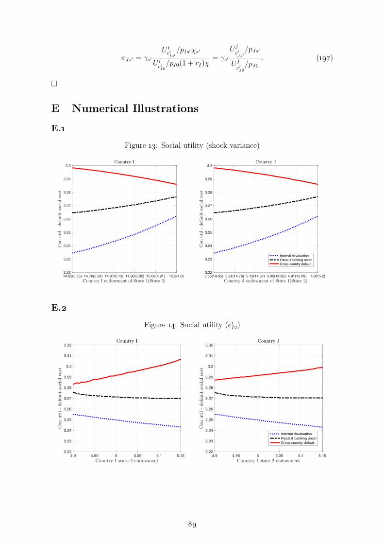
πJs′ = γs′U ici

Is′/pIs′χs′

U ici

I0/pI0(1 + rI)χ

= γs′U j

cj

Js′/pJs′

U j

cjJ0/pJ0

. (197)

�

E Numerical Illustrations

E.1

Figure 13: Social utility (shock variance)

14.65(5.35) 14.76(5.24) 14.87(5.13) 14.98(5.02) 15.09(4.91) 15.2(4.8)3.22

3.23

3.24

3.25

3.26

3.27

3.28

3.29

3.3

5.35(14.65) 5.24(14.76) 5.13(14.87) 5.02(14.98) 4.91(15.09) 4.8(15.2)3.22

3.23

3.24

3.25

3.26

3.27

3.28

3.29

3.3

Internal devaluationFiscal &banking unionCross-country default

E.2

Figure 14: Social utility (eiI2)

4.9 4.95 5 5.05 5.1 5.153.22

3.23

3.24

3.25

3.26

3.27

3.28

3.29

3.3

3.31

3.32

4.9 4.95 5 5.05 5.1 5.153.22

3.23

3.24

3.25

3.26

3.27

3.28

3.29

3.3

3.31

3.32

Internal devaluationFiscal & banking unionCross-country default

89