The Competitive and Welfare Effects of New Product Introduction: The

Case of Crystal Pepsi ∗

Wei Xiao†

Johns Hopkins University

JOB MARKET PAPER

November, 2008

Abstract

The introduction of new products is an important method of competition in many markets.Towards understanding its impact on competition and welfare, this paper estimates the effectsof Crystal Pepsi being introduced by PepsiCo.

Estimating a structural model of the soft drink market, the competitive effect is decomposedinto two parts: the effect on the prices of existing products from increased competition, and theeffect of having additional product variety. I find that firms’ profit and consumer welfare bothincreased in response to the introduction of Crystal Pepsi, with the price effect accounting fornearly 90% of the gain in consumer surplus. The introduction of Crystal Pepsi is also used asan experiment to test the competitiveness of the soft drink market. Evidence of price collusionis found.

In comparing the welfare impact of introducing Crystal Pepsi under price collusion andprice competition, I find that social welfare increases more under collusion. Under competition,rivals of PepsiCo increase prices and, consequently, a new product introduction actually harmsconsumers; at the same time, PepsiCo’s profit gain is smaller. This finding suggests that firmshave a stronger incentive to invest in R&D when they collude in price than when they competein price.

JEL CLASSIFICATION: L11, L13, L49, L66, O31

Keywords: New Product Introduction, Social Welfare, Market Structure, Random Coefficient Model

∗I am grateful to my advisors, Joe Harrington and Matt Shum, for their continuous encouragement and guidance.Special thanks to Ronald Cotterill, the director of the Food Marketing Policy Center at University of Connecticut,to make part of the data in this paper available. I would also like to thank participants in applied microeconomicseminar at Johns Hopkins and Southern Economic Association Annual Meeting for their comments and suggestions.All remaining errors are my own.

†Department of Economics, Johns Hopkins University, 3400 N.Charles Street, Baltimore MD 21218. Email:weixiao@jhu.edu

1

1 Introduction

New product introduction is a common phenomenon in many industries; cereal, beer, soft drink

and yogurt are a few examples. Consumers benefit from this continuous development of new

products. On the one hand, consumer welfare improves as the choice set expands because they

have more products with different attributes. This is called the variety effect. On the other hand,

the introduction of a new product enhances competition on the supply side and lowers the prices of

existing products, allowing consumers to enjoy the same utility through a lower level of expenditure

than when the new product does not exist. This is called the price effect. Of course, firms are

the driving force behind these developments. They introduce new products or brands to crowd the

product space, gain market share from rival firms, and to deter potential entry1.

Some papers have studied the effects of new product introduction in a discrete choice framework.

For example, Trajtenberg (1989) studied the social gains from innovation in computed tomography

(CT) scanners. Pakes et al (1993) used the discrete choice system to compute an ideal price index

for automobiles that accounts for new good introduction. Nevo (2003) also constructed a price

index that takes into account new product introduction and quality changes in the Ready to Eat

(RTE) breakfast cereal market. Petrin (2002) estimated consumer welfare and producer surplus

from minivan introduction using a random coefficient model complemented with micro moments.

Kim (2004) estimated the effects of new brands on incumbents’ profits and consumer welfare in

the U.S. processed cheese market. These studies all assumed a particular competition model,

mostly Bertrand Nash oligopoly, to estimate the effects of new product introduction2, so they

ignored the question of whether the assumed market structure is correct for the target industry. As

my findings indicate, different market structures may have different or even opposite implications

regarding welfare, so it is important to examine the competition model first, then analyze welfare

estimates.

Hausman and Leonard (2002) used retail scanner data from before and after new product

introduction to estimate the benefit to consumers from a new brand in U.S. bath tissue market.1See Schmalensee (1978).2This is partly because they normally only have the data for post-introduction period, and not enough for market

structure analysis.

2

They compared the “direct” and “indirect” estimates of price effect to assess the validity of the

assumed competition model.3 However, they employed Gorman’s two-stage budgeting approach,

which suffers from the two common problems of market-level demand systems: the inability to

incorporate micro information on consumers, and the restriction of substitution patterns between

products. 4

In this paper, I follow the discrete choice approach taken in Berry et al. (2004), which allows

flexible substitution patterns, and investigate the implicit competition behavior of firms in soft

drink industry to analyze the competition effects of the introduction of Crystal Pepsi. I use the

introduction of Crystal Pepsi as an experiment to infer the market structure and find that price

collusion best describe the competition behavior between firms. Then I quantify the change in

consumer welfare from the introduction of Crystal Pepsi in the soft drink market, decomposing it

into a variety effect and price effect. I also estimate changes in producer surplus, measuring the

extent of profit gains by the introducer and the pricing interaction between firms upon the launch

of new product under different competition patterns. I find that the launch of a new product

has different impacts on social welfare when firms compete in different ways. In particular, a new

product can bring more social welfare in a collusive market than an oligopolistic market. Under

oligopoly, non-introducing firms can take a ”free ride” to increase their prices upon the entry of

new product to gain more profit, which would not happen in a collusive market, and this price

effect would eventually hurt consumers.

The rest of the paper is organized as follows. Section 2 describes the U.S. soft drink market

and the introduction of Crystal Pepsi. Section 3 introduces the demand and supply model used for

the analysis. Section 4 describes the data and outlines the estimation strategy. Section 5 presents

the empirical results of the model estimation and the counterfactual simulations, and I conclude in

section 6.3Direct price effect is the estimates of price reductions for existing products using pre- and post-introduction data.

Indirect price effect is to use only post-introduction data to simulate the prices without new product and estimatethe price effect of new product.

4Nevo(1997) estimates the multilevel demand system and mixed logit model from one dataset of RTE cerealmarket. The multilevel demand model yields some ”disturbing” cross-price elasticities and strange implications,while mixed logit model produces reasonable results.

3

2 The Soft Drink Industry and Crystal Pepsi Introduction

In 2006, the U.S. market consumed 4.89 billion gallons of soft drinks through retail chains, gen-

erating $16.3 billion in revenue5. Simmons National Consumer Survey in 2006 shows that more

than 80% of the population drinks carbonated beverages, and among those who drink, the average

amount of consumption in the last seven days is more than 5.5 glasses.

The soft drink industry is highly concentrated. The market share of Coca-Cola, the number-one

manufacturer, was 38.3% in 2006, followed by PepsiCo with 32.2%. The three-firm concentration

(C3) was nearly 90%.

The soft drink industry is one of the most prodigious introducers of new brands or flavors.

As is typical of most new products, most new soft drink brands do not succeed6. However, by

introducing new brands manufacturer can take market share and profits from rivals, and at the

same time, the new brands crowd the product space and make the market more competitive, which

can lower the prices of existing brands and improve consumer welfare. As an example, I use the

introduction of Crystal Pepsi by PepsiCo in the early 90’s to examine the competitive effects of

new product introduction and its impact on consumer welfare.

Crystal Pepsi is a caffeine-free soft drink; it tastes like original Pepsi but it is colorless. In April

1992, PepsiCo began testing the market in Providence, Denver and Dallas with good feedback,

and in December Crystal Pepsi was distributed national-wide with a large marketing campaign.

After three months Crystal Pepsi captured a national market share of 2.4%, which is an excellent

performance according to industry criterion. But it fell quickly and ended up with the annual share

of 1.1% in 1993, and was pulled off the market in early 1994.

Since the data for estimation are prices set by the retailers, while my research question is about

manufacturers’ behavior, if the interactions between retailer and manufacturers are not taken into

account, the implications of the estimation results will be ambiguous.7 Here I review the marketing

chain from manufacturers to consumers in the soft drink industry.8 The soft drink marketing chain5Mintel Report on Carbonated Soft Drink 2007, and the retail chain exclude Wal-Mart.6Urban et.al(1983) shows that around 80% of new consumers goods introduction failed.7Many empirical studies on merger, new product introduction treat scanner retail prices as set by manufacturers,

so whether the implied effects are from retailers or manufacturers is not clear. For example, Dube (2005), Kim (2004)and Nevo (2000).

8Most of the contents in this paragraph are from Tollison, Kaplan and Higgins (1991).

4

comprises three parts: concentrate or syrup producers, bottlers, and retailers. Concentrate or syrup

producers are the firms that produce concentrate or syrup, the raw material used to produce the

finished soft drink products. Bottlers perform two major roles, the first is to purchase concentrate

or syrup, manufacture soft drink by mixing the syrup with carbonated water and other ingredients

and pack them into finished products ready to sell, and second is to deliver and market finished soft

drink products to the retailers.9 And retailers are firms such as grocery stores that make soft drinks

available to consumers. Historically, Coca-Cola Co. and PepsiCo produced the concentrate or syrup

and sold them to independent bottlers. However, from the late 1970s there was a trend of vertical

integration of bottlers by concentrate producers, and by 1993, 70.8% of Coca-Cola and 70.6% of

PepsiCo’s concentrate volume were distributed by their company-owned bottlers.10 For example,

PepsiCo manufactures concentrates and sells them to its own bottlers, as well as independent

franchise bottlers, throughout the United States, and the bottlers manufacture, distribute and

market finished soft drink products under PepsiCo trademarks.11

In a regional market, as the metropolitan area of my sample, bottlers compete with each other

for the trademarks they carry, and price discounting has been a major weapon. Among the soft

drink products sold in retailers, around 75% of the volume was sold at a discount price12, and the

costs of discounting were mainly borne by bottlers.13 Bottlers are offering price breaks and feature

ads based on numbers of cases sold and they even pay for shelf space.14

In this paper, the term manufacturer refers to the combination of concentrate producer and

bottler, and the results and conclusions should be explained accordingly.9Generally speaking, distributors lie between bottlers and retailers in the marketing chain, and this second function

is performed by the distributor, but in soft drink industry, bottlers take the roles of both parts.10See Saltzman, Levy and Hilke (1999) Table III.5.11PepsiCo bottlers, whether independently owned or company owned, generally manufacture and distribute soft

drink from other concentrate or syrup producers as well. This fact may contribute partly, but not much, to the pricecollusion conclusion I draw later.

12From Marketing Fact Book, 1983, 1986 and 1989 editions.13The price coupon and feature ads are normally on weekly basis, and the weekly prices variation mainly come

from this.14“The soda wars - a report from the battlefront”, US News and World Report, July 8, 1985, p58.

5

3 The Model

In this section, I present a structural model of demand and supply to evaluate the competitive

effects of the introduction of Crystal Pepsi. In contrast with the existing literature on soft drink

industry15, I tailor the framework of the BLP model16 to fit the market characteristics and to meet

the need for the analysis of Crystal Pepsi.

3.1 Demand

The core part of the model is to estimate the consumer’s demand, and the estimation of supply

and the following analysis of competition effects and welfare change all depend on this step.

Suppose there are J products, indexed by j, M consumers, indexed by i, M is the market size,

and we observe T weeks (indexed by t). The conditional indirect utility of consumer i from product

j in week t is

uijt = xjβ∗i + α∗

i pjt + ξjt + εijt ≡ Vijt + εijt (3.1)

where xj is a K-dimensional (row) vector of observable product characteristics, pjt is the price

of product j in week t, ξjt is an unobservable (by the econometrician) product characteristic, and

εijt is a mean-zero stochastic term. Finally, (α∗i β∗

i ) are K + 1 individual specific coefficients.

Examples of observed characteristics are calories, carbohydrates, sodium, caffeine and whether

the drink is clear. The unobserved characteristic covers all factors not included in the model

but affect consumer’s utility; we assume consumers observe it and then it can be interpreted as

consumer taste on that product. So, as ξjt can change over time, we can think of it as consumer

taste changing.

The specification given by (3.1) assumes that all consumers face the same product character-

istics. However, consumers with different demographics may have different preference for those

product characteristics; this is the motivation of the random coefficient model. I model the distri-

bution of consumers’ taste parameters for the characteristics as multivariate normal (conditional15For example, Gasmi et al.(1992), Cotteril et al. (1996), Dube (2005) and Chan (2006)16To my knowledge, this paper is the first one to apply BLP framework in soft drink industry.

6

on demographics) with a mean that is a function of demographic variables and parameters to be

estimated, and a variance-covariance matrix to be estimated as well. Let

α∗i

β∗i

=

α

β

+ ΠDi + Σνi, νi ∼ N(0, Ik+1)

where K is the dimension of the observed characteristics vector, Di is a d× 1 vector of demo-

graphic variables, Π is a (K+1)×d matrix of coefficients that measure how the taste characteristics

vary with demographics, and Σ is a scaling matrix. This specification allows individual charac-

teristics to consist of demographics that are “observed” and additional characteristics that are

“unobserved”, denoted Di and νi respectively. Substitute this into (3.1), we have:

uijt = δjt(xj , pjt, ξjt;α, β) + µ1ijt(xj , pjt, Di; Π) + µ2

ijt(xj , pjt, νi; Σ) + εijt

δjt = xjβ + αpjt + ξjt, µ1ijt = [pjt, xj ]

′ ∗ (ΠDi), µ2ijt = [pjt, xj ]

′ ∗ (Σνi)

The utility is now expressed as the mean utility, represented by δjt, and a deviation from that

mean, µijt + εijt, which are the effects of the random coefficient.

Specification of the demand system is completed with the introduction of an “outside good”;

the consumers may decide not to purchase any of the products. The indirect utility from this

outside option is

uiot = ξ0 + π0Di + σ0νi0 + εi0t

I assume that the consumer purchases one unit of the product that gives her the highest utility

and no tie exists.17 Then the probability that consumer i chooses good j in week t is given by

Prob(yijt = 1|Di, νi, εijt) = Prob(uijt > uilt,∀ l 6= j, l = 0, 1, . . . , J |Di, νi, εijt) (3.2)

The market share of product j in week t, as a function of the mean utility levels of all J + 117Hendel (1999) develops a multiple discreteness model in which consumers are allowed to purchase more than one

item. And see Dube (2005) for an application.

7

goods and the parameters, is given by

sjt =∫

Prob(yijt = 1)dF ∗(D, ν, ε) =∫

Prob(yijt = 1)dF ∗(ε)dF ∗(ν)dF ∗(D) (3.3)

where F (·) denotes the population distribution function. The second equality comes from the

assumption that the distribution of D, ν and ε are independent.

I further assume that εijt are i.i.d. with type I extreme value distribution. Then from (3.2), the

probability of consumer choosing product j at week t is

Prob(yijt = 1|Di, νi) =exp(Vijt)

ΣJtl=0exp(Vilt)

=exp(Vijt)

1 + ΣJtl=1exp(Vilt)

The second equality come from normalizing the mean utility of the outside good to be zero.

In my specification, νi is stochastic unobserved individual characteristics, so the above equation

produces a mixed logit model, which generate rich substitution pattern between choices. Or, it can

be written as

Prob(yijt = 1|Di) =exp(δjt + µ1

ijt + µ2ijt)

1 + ΣJtl=1exp(δlt + µ1

ilt + µ2ilt)

(3.4)

3.2 Supply and Equilibrium

Suppose there are F groups, each of them contains a subset, zf , of the j = 1, 2, . . . , J products.

The profit of group f ∈ F is

Πf = Σj∈zf(pj −mcj)Msj(p)− Cf

where sj(p) is the market share of product j, which is a function of prices of all products, M

is the market size, mcj is the constant marginal cost of product j, and Cf is the fixed cost of

production of group f . Then, under the assumption of pure-strategy Nash-Bertrand equilibrium,

the first order condition of group’s profit maximization problem becomes

8

∂Πf

∂pj= sj(p) +

∑r∈zf

(pr −mcr)∂sr(p)∂pj

= 0

When a multi-product group sets price for a single product, it maximizes the profit of all

products within the group. This effect is captured by the second term, which include the impact

of pj on both product j’s own price effect on its revenue and other products’ revenue inside the

group.

These J equations imply the marginal cost and price-cost margin for each product. For notation

convenience, define the matrix

Ωjr(p) = −∂sj(p)∂pr

, j, r ∈ J

and the market structure matrix

Λwjr =

1 if ∃f : r, j ⊂ zf

0 otherwise(3.5)

The market structure matrix Λw indicates the competition pattern behind firms. If firms

maximize the single product’s profit, Λw is an identity matrix; if firms compete oligopolistically,

zf covers all the products produced by firm f ; and if firms collude in price, Λw is a matrix with

all elements being one.

The first order conditions can be written as

s(p)− Ω(p). ∗ Λw(p−mc) = 0

where p, mc, s(p) are, respectively, the price vector for all products, the marginal cost vector

for all products, and the vector of market shares. This implies a markup equation and a marginal

cost equation

p−mc = (Ω(p). ∗ Λw)−1s(p) ⇒ mc = p− (Ω(p). ∗ Λw)−1s(p) (3.6)

9

I use equation (3.6) in two ways. First, I use the estimates of the demand system to compute

the marginal costs implied by (3.6). These estimates of marginal costs rely on obtaining the

consistent estimates of the demand system and on the assumption of equilibrium market structure.

Second, under the assumption that the marginal cost does not change and for the same equilibrium

structure, I simulate the counterfactual equilibrium prices that would have occurred were Crystal

Pepsi not introduced. That is, I replace the post-introduction market structure Λw in (3.6) with

the structure matrix of assumed market structure in pre introduction period, Λwo, and plug in the

estimated marginal costs. The predicted equilibrium prices without Crystal Pepsi solve

p∗ = mc + (Ω(p∗). ∗ Λwo)−1s(p∗) (3.7)

4 Data and Estimation

4.1 The Data

The data used for demand estimation is a scanner data set collected by Information Resource

Inc.(IRI), containing household-level soft drink purchase data and store-level sales data in 8 store

chains in a large metropolitan area. The sample period is 104 weeks from June 1991 to June 1993,

and Crystal Pepsi is present in the last 25 weeks. The household level data tracks 1024 household’s

soft drink shopping history with the information on shopping date, units and prices of products

purchased, store locations and household demographics. The store level data contains the weekly

prices and units sold for each available product, the promotion activity, and the total brands in

each week.

The product’s characteristics include calories, carbohydrates, sodium content and whether it is

clear. Those data are obtained from CocaCola and PepsiCo’s websites or supermarket packages 18.

4.2 Retailer and Manufacturer Interaction

This section discusses a few comments and assumptions about the role of retailers. As mentioned

before, the data used for estimation are the retail prices in the stores, however, my research question18Assuming the current brand’s contents are the same as in early 90’s

10

is about manufacturers’ behavior. As a bridge between manufactures and consumers, how does the

role of retailers fit into the model?19

I focus on the category of soft drink products, so if the retail chains compete with each other

in this category by optimizing their soft drink prices across all products, the inferred implications

from retail prices about competition models and market structures will be ambiguous on whether

the interaction is among manufacturers or retailers. In this case, I would have to incorporate the

retailers into the model in which manufacturers maximize their profits from the wholesale prices and

retailers choose the optimal retail prices based on the manufacturers’ wholesale prices. However,

if retailers do not compete with each other on the basis of a single product category (in this case,

soft drinks), I can reasonably assume that retail prices are determined non-strategically, retailers

take the manufacturers’ wholesale prices as given, and the strategic pricing is among manufacturers

only.

Slade (1995) interviewed managers of grocery stores who report that the majority of consumers

do not engage in across-store price comparisons for a given brand. Instead, the price comparison

is usually across different manufacturers or brands within a store. Slade empirically tests this

argument in the product category of saltine crackers with positive results. In addition, Walters

and Mackenzie (1988) find evidence that there is often no strategic interdependence among retail-

ers with respect to the pricing of brands within a particular product category. Moreover, if the

manufacturer is the Stackelberg price leader in the retailer-manufacturer interaction game, and if

retailers do not compete with each other on the category, Sudhir (2001) shows that the measure of

coordination or the competitiveness among products is equivalent between two models: the retailer

coordination model, in which the retailer coordinates the prices of the target product category ig-

noring manufacturers; and the constant margin retailer model, in which the competition is among

manufacturers and retailers play non-strategically with a fixed markup.20 Therefore, the observed

retail prices could be used to analyze manufacturers’ behavior.

Given the preceding discussion, I assume that retailers set the prices of soft drink products by19Many studies using supermarket scanner data assume that the observed retail prices are set by the manufactures

without rationales, for example, Dube (2005), Kim (2004) and Nevo (2000).20In other words, if the retailer sets the prices to maximize the profit of each single product, from econometric

pointview, this is equivalent to the scenario that manufacturers’ strategy is to maximize single product profit andthe retailer charge a constant margin.

11

the fixed markup rule. Thus, incorporating the retailer explicitly does not change the model stated

previously significantly. To see this, suppose wjt is the wholesale price of product j in week t, and

P rjt is the retail price, then

P rjt = wjt + rjt

where rjt is the retailer mark-up. When retailer applies a fixed mark-up rule, we have:

rjt = m ∗ wjt

Hence,

P rjt = (1 + m)wjt

When manufacturers choose the wholesale prices wjt to maximize their profit and the retailers

set the retail prices by fixed mark-up rule accordingly, the system of demand and supply equations

remain the same as that without an explicit retail chain, except the adjustment of marginal costs,

which would be divided by a factor (1+m).21 Note that m cannot be identified in the estimation and

its value has to be given exogenously using empirical information on retailer’s mark-up. However,

the exact retail mark-ups are generally not available and have to be estimated from the observed

retail prices, which are not accurate and vary under different assumptions.22 In addition, the

demand parameter estimates, price-cost margin ratios, price elasticities and welfare changes are

not affected by the incorporation of retailer price setting behavior.23 As a result, I do not make a

distinction between manufacturer and retailer prices.21This can be seen from (3.6) and (5.1).22Barsky et al. (2001) estimated that the retailer’s markup on national’s brands in soft drink category is between

14% and 37%.23Except that the price coefficients and the absolute level of welfare changes will be discounted by a factor (1+m),

but the sign and significance will not change.

12

4.3 Model Estimation

In this section I describe the procedure I use to estimate the consumers’ demand. The parameters

to be estimated are α, β, the coefficient matrix Π and the scale matrix Σ. I employ the generalized

method of moments (GMM) with both the market share and micro moments that follows Berry

et al. (2004). The essential idea is to form the GMM objective function as an interaction of the

instruments and a value of unknown parameters, which is an error term computed from the model.

4.3.1 The Micro Moments

The idea for using micro moments originally comes from Imbens and Lancaster (1994), and has

been used by Berry et al. (2004) and Petrin (2002). The motivation is that the macro data can be

viewed as the aggregate of micro data, and the aggregate data may contain useful information on

the average of micro variables, so combining both the macro and the micro moments can improve

the accuracy of the estimation.

I have the household level purchase data, so I can search for the parameters that match the

average model predictions of households’ demographics conditional on purchasing a specific brand

to the observed averages from the data set. Formally, the micro moments can be written as

G1(θ) =∑

j

(nj/n)xkj1/nj

nj∑ij=1

Dij − E[D|yi = j, β, ν] (4.1)

where nj is the number of households who purchased product j, xkj is the kth characteristic

of product j, Dij is the demographics of household i who purchase product j, and yi = j is an

indicator function for household i purchasing product j.

Notice that we cannot calculate the conditional expectation E[D|yi = j, β, ν] directly, so I

approximate it by Bayes’ rule to write it as

E[D|y = j, β, ν] =∫

DDdP (D|y = j, β, ν) =

∫D DPr(y = j|D,β, ν)dP (D)

Pr(y = j, β, ν)

and substitute from model’s predictions for choice probabilities (3.4) to obtain

13

E[D|y = j, β, ν] =

∫D

∫ν DPr(y = j|D,β, ν)dP (v)dP (D)

Pr(y = j, β, ν)(4.2)

To calculate the probabilities, Pr(y = j|D,β, ν) and Pr(y = j, β, ν), in (4.2), I need the

model parameters θ and the mean utility δ. θ is the parameters to be estimated from the moment

conditions, while I substitute the δ here with the one estimated from the market share moments

by contraction mapping. In doing so, for each value of β, Pr(y = j, β, ν) will equal the observed

market share sj . On the other hand, the integral in the numerator of (4.2) has to be simulated.

By taking random draws of (Dr, vr), I can approximate (4.2) as

E[D|y = j, β, ν] ≈(ns)−1

∑r DrPr(y = j|Dr, vr, β, δ(β))

sj(4.3)

The micro moments are formed by substituting (4.3) into (4.1). Since I have two demographic

variables (income and family size) and six product characteristics (constant, price, advertisement,

caffeine dummy, clear dummy and package dummy), there will be 2 × 6 = 12 micro moments in

total.

4.3.2 Moments from Market Share

Let Z = (z1, . . . , zM ) be a set of instruments, and ω is a function of the model parameters, which

will be defined below as an error term. The second set of moments can be written as

G2(θ) = E[Z′ · ω(θ∗)]

where θ∗ denotes the true value of those parameters.

I define the error term as the unobserved product characteristics, ξjt . To computer these

unobserved characteristics, I first solve the mean utility level δ·t from the system of equations

s·t(x, p, δ·t; Σ) = S·t (4.4)

14

where s·t is the market share function of all products in week t defined by (3.3), and S·t is the

observed market share. Once δjt is solved, the error term, ξjt, is defined as δjt(x, p, S·t; Σ)− (xj β +

αpjt), here α and β are estimates from the regression of δjt on xj and pjt.

To solve this system of equations I need to find the market share function. The market share

is defined by (3.3). I assume ε follows the type I extreme value distribution, so the market share

becomes

sjt =∫

exp(Vijt)

1 +∑Jt

l=1 exp(Vilt)dF ∗(ν)dF ∗(D) (4.5)

If I further assume ν ∼ N(0, IK+1), and obtain the empirical distribution of D, I can approxi-

mate the above integral from direct Monte Carlo simulation by

sjt(p·t, x·t, δ·t; Σ) =1ns

ns∑i=1

sijt

=1ns

ns∑i=1

exp[δjt +∑K+1

k=1 xkjt(

∑dh=1 πkhDih) +

∑K+1k=1 xk

jt(∑K+1

l=1 σklvkil)]

1 +∑J

m=1 exp[δmt +∑K+1

k=1 xkmt(

∑dh=1 πkhDih) +

∑K+1k=1 xk

mt(∑K+1

l=1 σklvkil)]

where i = 1, . . . , ns are draws from P ∗(ν) and P ∗(D) respectively. xkjt, k = 1, . . . ,K + 1, are

product characteristics including price that have random slope coefficients.24

Clearly, with the computation of market share under current full random coefficient model, the

mean utility δ·t does not have an analytical solution from the equation system (4.4). As suggested

by Berry et al (1995), they are solved numerically by using the contraction mapping, which is to

computing the series

δh+1·t = δh

·t + lns·t − lns(p·t, x·t, δh·t; Σ), h = 1, . . . ,H (4.6)

where s(·) are the predicted market shares from above simulation, H is the smallest integer

such that ‖δH·t − δH−1

·t ‖ is smaller than some tolerance level, and δH·t is the approximation to δ·t.

For the estimation in this step, I treat each week as a separate market and use the average24Here I abuse the notation to include price into x, while in the model x and p are denoted separately. However,

the meaning is clear here and the equation is simplified with this abuse.

15

weekly price as the price set by manufacturer. These are strong assumptions, since my data sample

contains only one metropolitan area, and the demographic distribution is the same for every week

(or for every market). I make different draws for each week, so the variation in market share comes

not only from the prices and other varying characteristics but also from the random draws of the

distribution of unobserved demographics, ν, and its coefficient matrix Σ.25 The economic meaning

of ν will not be limited to unobserved demographics of individuals, it explains the variation of

both observed and unobserved demographics that cause the variation in market share from week

to week.

4.3.3 The Objective Function

The two sets of moments that enter the GMM objective function are G1(θ),the micro moments

associated with household level data, and G2(θ), the market share moments associated with store

level data. The population moment conditions are assumed to equal zero at the true value of θ, or

E[G(θ)] = E[G1(θ);G2(θ)] = 0

Following Hansen (1982), the efficient GMM estimate is

θ = argminθG(θ)′W−1G(θ) = argminθG

∗(θ)′G∗(θ)

where W is the weight matrix that is a consistent estimate of the asymptotic variance-covariance

matrix of the moments, and G∗(·) is the “square root” of W times G(·). By using the variance-

covariance matrix of the moments, we give less weight to those moments that have higher variances.

Let Γ = E[∂G∗(θ)/∂θ], the gradient of the moments with respect to the parameters evaluated

at the true parameter values, and let V = E[G∗(θ)G∗(θ)′]. The asymptotic variance of√

n(θ − θ)

is then given by

(Γ′Γ)−1Γ′V Γ(Γ′Γ)−1

25I tried one set random draws of ν for all weeks, here the variation of market share only comes from the changesin varying product characteristics, the estimation results are similar.

16

Reported standard errors are calculated using the consistent estimates Γ(θ) and V (θ).

4.3.4 Instrument

The consistent and efficient estimation of the mean utility δ(β) from the second set of moments

relies on the valid instrument variables that satisfy two requirements. First, they are uncorrelated

with the the error term of the model, or the unobserved product characteristics, ξjt. Second, they

are correlated with the price, pjt.

I use two sets of instrument variables. The first set is the total number of brands available

in consumer’s choice set, which varies over weeks due to entry and exit of brands and over stores

due to the generic products. The number of brands is an indicator of ‘crowdedness’of product

characteristics space and is a measure of the intensity of the competition a single product faces

in that week, so it will be correlated with price since the markup of each product depends on the

competition intensity and the distance from the nearest product on characteristic space. On the

other hand, the number of brands in each week is purely firm’s behavior, and it is likely to be

exogenous to unobserved product characteristics.

Since an alternative explanation of the error term is the consumer’s taste towards products, one

may argue that the decision of a firm to introduce a new brand is to satisfy those tastes. In this

case, the number of brands will be correlated with the error term. I would say that it is more sound

to argue that the firm’s decision of new product launch depends on the overall population taste on

soft drink market level, and when it comes to consumer’s taste for a single product, this correlation

will be weak if it exits at all. Another concern about this instrument is that the variation of number

of brands in the store does not come from manufacturers’ introducing new products, but from the

retailer’s decision on shelf space. If so, the number of brands on the shelf does not indicate the

competition intensity among manufacturers.26 To address this concern, imagine that in a single

store, the number of brands is what the consumers would choose from, and it is a measure of

competition intensity in that store. When the retailer changes the number of brands in the store,

it will adjust the prices accordingly. Since I assume retailers employ the fixed mark-up rule to26For an extreme example, if manufacturers’ brands remain the same over thewhole sample period, and the number

of brand in the data set varies because stores add to or remove brands from the shelf week by week.

17

set the retail price proportional to manufacturer’s wholesale price, the price change is attribute

to manufacturers even if it is retailer’s decision. Even though this is a simplified assumption on

retailer-manufacturer interaction, it makes this instrument valid. In addition, as mentioned in

Section 2, bottlers of different trademarks compete with each other in local markets by discounting

price and even paying for the shelf space, which is the main source of weekly price variation,27

so the number of products in stores indicates the competition intensity and is correlated with the

prices, while this competition is not correlated with unobserved product characteristics.

The second set of instrument variables comes from exploiting the rich panel data; they are the

prices of rival firms’ products in the past. For example, for ξjt of PEPSI BOTTLE 67.6 oz in first

week of 1993, the average price of Coca-Cola and Cadbury Schweppes in the first week of June 1991

can be the instrument. This instrument is valid under the assumption that the consumer’s taste

changes over time. In the soft drink market, this is not unusual, for example, in the early 90’s, diet

beverages gained popularity and clear products (including Crystal Pepsi) were advertised heavily,

affecting consumer’s preference. In addition, consumer demand fluctuates in different seasons like

winter and summer.28 Given this, the price of rival firm’s products in past different season is

exogenous to consumer taste, or the unobserved characteristics. At the same time, the rival firm’s

past price will be correlated with current product price, since in one city, all firms share some

same cost, such as transportation cost and cost to put the products on the same retail chain. For

the products’ characteristics are constant over time, the prices are also correlated from the direct

competition in same area.

Here are some notes on the instruments. First, I use both the number of brands and number of

UPC’s as instruments in the estimation. The argument for number of UPC’s as valid instruments

is similar to number of brands. Second, the first set of instruments varies across weeks but not

products, while the second set of instruments varies across products but not weeks. Using each

single set of instrument would not identify the parameters since they lack variation in one dimension,27In my sample, around 33% of the soft drink UPC’s were sold on discount from either feature or display in the

post introduction period.28For example, the average weekly market share of regular Pepsi in the sample followed a cyclical pattern over

seasons. The market share in the summer are obviously higher than in spring, in the summers from 1991 to 1993,the average weekly market shares are 11.5%, 9.6% and 11.7%, while in the springs of 1992 and 1993 are 7.6% and8.2% respectively. This indicates that consumers prefer Pepsi more in the summer than in the spring.

18

but by combining two sets of instrument together, I have the variation across both products and

weeks. It is this two-dimensional variation that identifies the demand parameters.

4.3.5 Measuring the Welfare and Profit Effects

To measure the effects of Crystal Pepsi’s introduction, I implement a counterfactual simulation

without Crystal Pepsi and estimate the consumer’s surplus and firms’ profit in 25 week after Crystal

Pepsi was launched. I simulate the counterfactual equilibrium prices from (3.7) with the new

structure matrix Ωwo(·), assuming the marginal costs do not change. And in the new equilibrium,

the market shares change accordingly with the new price vector.

Then I estimate the change of profit for each firm by computing the simulated profit without

Crystal Pepsi, and comparing with the profit with Crystal Pepsi.

∆Πf =T∑

t=1

[Πtf (p1,mc; θ)−Πt

f (p0,mc; θ)]

where Πtf (p1,mc; θ) is firm f ’s profit at the post-introduction equilibrium price p1 and Πt

f (p0,mc; θ)

is firm f ’s profit at the counterfactual equilibrium price p0. So, ∆Πf measures the firm’s profit

change from the introduction of Crystal Pepsi. The total supplier’s surplus change is the sum of

those profit changes.

Consumer welfare is measured by the compensating variation (CV), which is the dollar amount

a consumer needs to be compensated in the equilibrium without Crystal Pepsi to attain the same

utility level as in equilibrium with Crystal Pepsi. If the marginal utility of income is fixed for each

consumer, McFadden(1981) and Small and Rosen(1981) show that the compensating variation for

individual i can be written as

CVi =ln[

∑Jj=0 V w

ij (p1)]− ln[∑J−1

j=0 V woij (p0)]

α∗i

(4.7)

where V wij (p1) represents the utility level of individual i from product j at the equilibrium

price p1 with Crystal Pepsi as defined by (3.1), and V woij (p0) is the utility at the counterfactual

equilibrium price without Crystal Pepsi. α∗i is defined in (3.1) and is the marginal utility of income.

19

The compensating variation can be decomposed into two parts for two different effects, the

variety effect and the price effect.

CVi = CV vei + CV pe

i (4.8)

=ln[

∑Jj=0 V w

ij (p1)]− ln[∑J−1

j=0 V woij (p1)]

α∗i

+ln[

∑J−1j=0 V wo

ij (p1)]− ln[∑J−1

j=0 V woij (p0)]

α∗i

The first part is the variety effect of compensating variation, which captures the consumer’s

welfare change when removing the Crystal Pepsi from the actual equilibrium but keeping the

equilibrium prices fixed. The second part measures the price effect: the welfare change in a market

without Crystal Pepsi but the prices move from the counterfactual equilibrium level to actual

equilibrium level.

The total consumer’s compensating variation is given by the integral over the population

M

∫CVi(·)dP ∗(D)dP ∗(ν)

5 Results

5.1 Descriptive Statistics

In soft drink market, there are many brands and each brand has various package sizes. Every

combination of brand and package size is identified as a UPC in the data set, which adds up to

more than one thousand UPC’s in the market. Obviously, it is unrealistic to include all the UPC’s

in the model. Instead, I choose the top 45 UPC’s with the largest market shares, and define a

product by brand and an indicator of large package with 288 OZ, which ends up with 26 products

for my model. The characteristics of those products are reported in table 1 29 . In the sample

period, large bottle Pepsi has the biggest market share of 2.37%, Crystal Pepsi has the highest

price of 0.90 dollar per 32 fluid ounce, and the most advertised brand is Diet Coke. Before the

entry of Crystal Pepsi, the clear brands are 7UP, Canada Dry and Sprite, and small package 7UP29Calories, carbohydrates and sodium are the common ingredient of soft drink, and I tried including them in the

estimation but it turns out that they have very little effect on the demand, so I exclude them in the reported results.

20

has the biggest market share of 2.04%.

Table 2 summarizes the income and family size of households in the sample, the mean annual

income is $35, 700 and the mean family size is 2.66 . And Table 3 reports the average demographics

of purchasers for each product, which shows that the average income of Crystal Pepsi purchasers

is $37, 300 and the average family size is 3.18, both are higher than the population mean.

5.2 Parameter Estimates

Table 4 and 5 present the results from four different demand-side models: ordinary least square

(OLS) logit, logit model with instrumental variables, conditional logit with fixed effect, and random

coefficient model with micro moments. In Table 4, the size of estimated price coefficient decreases

significantly from OLS to instrumental variables, which is similar to Berry et al.(1995) and Petrin

(2002)’s findings, indicating that instrumental variables are important in the final specification.

The OLS and IV logit models restrict the parameters of interaction terms and random coefficients

in Table 4 to be zero. As many interaction terms and random coefficients are significantly different

from zero, the Wald test is to reject OLS or IV in favor of the more flexible framework.

Columns 2 and 3 of Table 5 report the demand coefficient estimates and their standard errors

from a conditional Logit model with fixed effect. The household data tracks what households

purchase in each week from what store, while the store level data contains the prices of available

products for each store in every week. I match each household’s shopping trip with the available

products of the store in that week to form a group.30 Then I run the fixed effect logit on those

groups using maximum likelihood estimation.31 Most parameters are significant and all the primary

parameters of product characteristics are highly significant with expected signs.

Conditional logit model exploits the information of households’ demographics and the charac-

teristics of products they directly choose from, however, this model assumes that the error term

follows the logistic distribution, and as a consequence, the unobserved consumer taste variation

over weeks is assumed away. I use the results from conditional logit as a benchmark to check with30For example, household x purchased product i at store y in week t, and store y had m soft drink products on

the shelf, so I know that household x chose item i from those m products, this forms a group.31The fixed effects are for groups, and the likelihood is calculated relative to each group, i.e. conditional likelihood

is used.

21

the demand estimates from the final specification. Columns 4 and 5 in Table 5 are estimated from

the random coefficient model with micro moments stated in the paper, and compared with columns

2 and 3, the coefficients of product’s characteristics and the interaction terms with demographics

are significant and of the same sign as conditional logit except two out of eleven. Thus the random

coefficient model combining the micro moments from household level data and the moments from

market level data provides reasonable and significant estimates of demand for the analysis of social

welfare and market structure.

5.3 Elasticities and Substitutes

There is no analytical expression for demand elasticities, so I numerically compute the own and

cross price elasticities of market share for all the products. From (4.5), the elasticity of product j

to product h is

ηjht =∂sjtpht

∂phtsjt=

−pjt

sjt

∫αisijt(1− sijt)dF ∗(D)dF ∗(ν) if j = h

phtsjt

∫αisijtsihtdF ∗(D)dF ∗(ν) if j 6= h

(5.1)

where sijt = P (yijt = 1) = exp(Vijt)

1+∑Jt

l=1 exp(Vilt). The integral is obtained from direct Monte Carlo

simulation. And ∂sjt

∂phtwill be used in (3.5) to estimate the marginal cost.

I compute the elasticities for each market and report the median of own and cross price elas-

ticities for a sample in Table 6.32 Own price elasticities are between −3.36 and −8.37, which are

reasonable compared to the estimates in other studies of the soft drink industry reported in Table

7. The elasticities demonstrate that for some brands consumers tend more to substitute between

products of the same size than to other sizes of the same brand. For example, demand for large

Diet 7UP is more sensitive to the price of large Pepsi (0.40) than to the price of small Diet 7UP

(0.05). This result is consistent to the findings by Guadagni and Little (1983) and Dube (2005)

that households tend to switch among products of the same package size.32The complete set of elasticities is available in a separate appendix.

22

5.4 Examination of Market Structure

One advantage of the model is that I can simulate the prices without Crystal Pepsi under different

scenarios of market structure. As I have the data of prices before introduction, the comparison of

actual prices with the simulated prices without Crystal Pepsi could shed light on the competition

pattern between firms. The actual and simulated prices change due to the introduction of Crystal

Pepsi should be approximately equal if the demand system is correctly specified, the firms’ marginal

costs are constant over the sample period and over the relevant range of output, and the assumed

model of competition is correct. The random coefficient model used for demand system is flexible,

and the estimates are reasonable and robust comparing to alternative specifications, in addition,

the price changes are relatively small, so misspecification of the demand system is unlikely to be

substantial if it exists at all. In the same way, for relatively small quantity changes, the marginal

cost changes are not likely to be large unless firms are operating at near full capacity. Other reasons

that could cause big changes in marginal cost are production efficiency improvements or local labor

cost variation, however, given that the sample length is only two years in a single metropolitan area,

substantial marginal cost changes are not likely to happen. Thus, neither of the first two potential

reasons should lead to a substantial difference between actual and simulated prices without Crystal

Pepsi, and consequently, the finding of a substantial divergence between two sets of prices would

suggest the failure of the assumed model of competition to accurately describe the true firms’

behavior.

I access three alternative models of competition for both pre and post introduction of Crystal

Pepsi to examine which simulated price changes match the actual price changes closest. I consider

three market structures: oligopoly price competition, in which each firm sets the prices to maximize

profit; perfect price collusion, in which the prices of all products are set by a cartel; and single

product pricing, in which prices are set to maximize each single product’s profit. Since either pre or

post introduction period can be one of those three structures, there are nine possible combinations.

For example, firms may collude in price before the introduction of Crystal Pepsi, but they become

oligopoly competing in price in post introduction period. It is worth noting that the marginal cost

estimates depend on the assumed model of post introduction period, thus for each combination,

23

I hold the marginal cost constant from the post introduction estimates, and simulate the prices

without Crystal Pepsi from the assumed pre-introduction market structure.

Columns 2 and 3 of table 8 report the mean and standard error of weekly median actual and sim-

ulated prices of 26 products, and column 4 presents the paired t-statistics of the null hypothesis that

the actual percent price changes of all products from pre to post introduction are the same as sim-

ulated one. Of the nine alternative competition models, simulated prices from collusion/collusion

model stand out to be reasonably close in magnitude and not statistically significantly different

from zero compared to the actual prices without Crystal Pepsi. And oligopoly/oligopoly model

rejects the null hypothesis at 6.2% level. All other assumed competition models reject the null

hypothesis significantly with absolute value of t-statistics greater than 833.

This finding is different from Gasmi et al. (1992) whose evidence does not support collusive

pricing in the soft drink industry. However, Gasmi et al. (1992) employs the reduced linear demand

equations, limits itself to interactions between two firms (CocaCola and PepsiCo) and aggregates

each firm’s differentiated brands as one single product. This simplification is questionable because

each single brand is priced and advertised separately to meet corporation goal.34 Compared to the

aggregate linear market-level demand system, random coefficient logit model distinguishes different

brands, considers more than two manufacturers and exploits the interactions between consumer

preferences and product characteristics, which leads to more realistic substitution pattern, and

consequently allows richer strategic interaction among firms.

In addition, the aggregation in Gasmi et al (1992) is equivalent to assuming that each firm

maximizes its profit over all brands and then testing whether cooperation exists among duopoly,

while in this paper, I evaluate all three possible market structures. So I am confident that the

finding in this paper about the existence of price collusion is more reliable.35

33The degrees of freedom is 24.34I do not say the goal is to maximize firm’s overall profit, because this is one of the hypotheses I will examine.

The possible goals could be maximizing single brand’s profit, maximizing the whole market profit (collusion) ormaximizing firm’s overall profit (oligopoly).

35Actually, the adjusted LR statistic in Gasmi et al (1992) does not reject the price collusion significantly.

24

5.5 Changes in Consumer Welfare

As stated in section 4.3.5, I use compensating variation to measure changes in consumer welfare

from the introduction of Crystal Pepsi. In the counterfactual scenario, there is no Crystal Pepsi, and

other soft drink prices solve the set of equilibrium first order conditions in (3.7). For consumers

not purchasing Crystal Pepsi, the compensation is determined entirely by the changes in soft

drink prices associated with the entry of Crystal Pepsi. Households benefits more from purchasing

products whose prices decrease more. Table 9 summarizes the median current prices and the

counterfactual prices without Crystal Pepsi under the collusion model. It shows that Crystal Pepsi

products were substitutes to all existing clear brands, in particular, large 7UP and large Diet 7UP

experienced the largest percentage price decreases. In addition, large Caffeine Free Diet Pepsi,

large Pepsi, large Coke Classic, RC and all Dr Pepper products decreased their price upon the

entry of Crystal Pepsi. Specifically, large Pepsi’s price was reduced by nearly 12%, this shows the

cannibalization effect of new product on introducer’s existing brands. As reported in Table 11,

the estimated gains to non-Crystal Pepsi purchasers from increased price competition account for

almost 89% of total consumer benefits, and if measured in per 32 fluid ounce serving of soft drink,

the price effect is 0.55 cents.

For Crystal Pepsi purchasers, welfare change is the dollar amount that a Crystal Pepsi consumer

needs to be compensated at the new equilibrium prices to achieve the “Crystal Pepsi standard of

living”. The variety effect is measured as the first term in (4.8), which is 0.07 cents per 32 fluid

ounce serving and accounts for 11% of total consumer surplus.

5.6 Profit Dissipation and Total Welfare Change

Before turning to measure the firms’ profit change, I compare the markups of all products with

and without the entry of Crystal Pepsi. Table 10 reports the estimated marginal costs and the

margins. The third column of post-introduction margins indicates that carbonated soft drink is a

high profit industry, the average markup is 43%, large Pepsi has the highest markup of 58%, while

the new introduced product Crystal Pepsi has the lowest markup of 29%. The fact that Crystal

Pepsi has the highest marginal cost and lowest markup shows that introducing a new product is

25

costly for firms.

Upon the entry of Crystal Pepsi, six out of seven clear products decreased their margins,

specifically margins of large Diet 7UP and large 7UP decreased by more than 10%, which is the

largest decreases of all products. The only exception is small Diet 7UP whose margin increased

by 1%. Among seven PepsiCo products (excluding Crystal Pepsi), margins of four increased and

three decreased. This illustrates that Crystal Pepsi competed more with other clear brands while

the effect on introducer’s brands was mixed.

Changes in PepsiCo and all firms’ variable profit due to the introduction of Crystal Pepsi are

reported in row 2 of Table 11. These estimates are obtained by computing implied profits without

Crystal Pepsi and comparing them to the profit with Crystal Pepsi using the median prices over

weeks. Results suggest that PepsiCo benefited significantly from introducing Crystal Pepsi, as

variable profits increased by $5, 052.07 per week in the sample relative to what profits would be

without the introduction.36 Other manufactures benefited as well from PepsiCo’s innovation, their

weekly profit in sample increased by $1, 301, which is an increase of 12% of their total profit37. Total

profit of firms were increased by $6, 353, approximately 38% of the profit were Crystal Pepsi not

introduced. However, the introducer, PepsiCo, took most profit benefits (80%) from the innovation.

Social welfare is the sum of consumer surplus and producer welfare, which add up to $7, 879

per week in the sample. Around 81% of the social welfare surplus went to producers, however, in

particular the introducer of Crystal Pepsi, this shows that firms have incentive to keep introducing

new brands to gain more profit. For consumer surplus, purchasers of Crystal Pepsi gained positive

utility from the characteristics of the new product, while most benefits went to non Crystal Pepsi

consumers due to price reduction.

5.7 Market Structure and Welfare

The results reported in preceding sections are under the competition model of collusion that best

matches the observed data. However, the oligopoly competition model is not unreasonably far36The profit increase is 87.6% of PepsiCo’s profit if not introducing Crystal Pepsi. This number is huge at first

glance, but I only include the products of PepsiCo in the model that are most correlated with Crystal Pepsi, so thisratio is over estimated of the actual percentage increase.

37For the same reason that only part of the products are included in the model, the number here only illustratethe change in the sample.

26

in magnitude and not statistically significantly different from zero according to the t-test. Here

I simulate the equilibrium prices and the social welfare change under the price competition of

oligopoly, and compare them to the results from the collusion model to investigate the effects of

new product on social welfare under different market structures. This exercise would illustrate the

incentive of firm’s innovation and its impact on social welfare under different antitrust policies.

The welfare changes from oligopoly competition are reported in the first row of Table 11. The

consumer surplus from the variety effect remains the same and the profit increase for new product

introducer PepsiCo is smaller than in collusion case. However, contrary to the collusion model,

the price effect of consumer surplus is dropped to −$1, 405 from $1, 352 and the rival firms’ profit

improvement rises from $1, 301 to $2, 162. As a result, total consumer welfare would decrease

from the introduction of Crystal Pepsi if firms competed in oligopoly, while total social welfare

improvement is reduced to $5, 090, which is around 35% decrease from collusion model.

The above comparison shows that when a firm in a cartel introduces a new product, consumers

benefit from the innovation, and both the innovator firm and other producers’ profit increase. On

the other hand, when a firm introduces new product in oligopolistic market, introducer will gain

less profit and the rival firms could take a “free ride” on the innovation to raise prices for more

revenue, while, surprisingly, consumers would be hurt from the innovation.

6 Conclusions

This paper examines the effects of introduction of Crystal Pepsi in the soft drink market on con-

sumer welfare and firms’ profits. The effects of new product introduction in carbonated soft drink

market has not been analyzed formally before using a random coefficient model combining house-

hold level and store level data.

The estimation results of logit models indicate that controlling for price endogeneity is important

in this market. The price coefficient estimates increase significantly by using instrumental variables.

The results from a random coefficient model show that advertising has significantly positive effects

on demand, but this effect decays as household income increases.

Comparing the price effect of Crystal Pepsi introduction from counterfactual equilibrium under

27

various competition models to the actual price effect, the price collusion model best describes the

firms’ behavior. Under the collusion model, the new product increased consumer’s welfare mostly

by the price effect due to the price reduction from the entry. The new product helped the introducer

PepsiCo to capture the combined market share and increase its profit. And the profit of other firms

increases as well from the introduction of the new brand.

Simulated equilibrium from the oligopolistic model demonstrates that non-introducing firms

would raise their prices upon the entry of the new product and gain more profit, and at the

same time, the introducer would capture less profit than in the collusion model. Surprisingly,

consumers would be hurt from the innovation if producers compete in oligopoly. The social welfare

improvement is still positive from the innovation but is lower than in a collusive market.

My results suggest that the innovation in a collusion market will bring more social welfare

improvement. Firms in an oligopolistic market would have less incentive to invest in R&D and

innovation because they can take “free ride” by increasing prices to gain profit when other firms

introduce new products.

28

References

[1] Barsky, R., Bergen, M., Dutta, S. and Levy, D., “What Can the Price Gap Between Branded

And Private Label Products Tell Us About Markups?”, NBER Working Paper 8426, (2001)

[2] Benedetto, C Di., “Identifying the Key Success Factors in New Product Launch ”, Journal of

Product Innovation Management, Vol. 16 (1999), pp. 530-544

[3] Berry, S., “Estimating Discrete Choice Models of Product Differentiation ”, RAND Journal of

Economics, Vol. 25 (1994), pp. 242-262

[4] Pakes, A., Berry, S., and Levinsohn, J. “Applications and Limitations of Some Recent Ad-

vances in Empirical Industrial Organization: Price Indexes and the Analysis of Environmental

Change”, American Economic Review, Vol. 83 (1993), pp. 247-52

[5] Berry, S., Levinsohn, J., and Pakes, A., “Automobile Prices in Market Equilibrium”, Econo-

metrica, Vol. 63 (1995), pp. 841-890

[6] Berry, S., Levinsohn, J., and Pakes, A., “Differentiated Products Demand Systems from a

Combination of Micro and Macro Data: The New Car Market ”, Journal of Political Economy,

Vol. 112 (2004), pp. 68-105

[7] Chan, T., “Estimating A Continuous Hedonic Choice Model with An Application to Demand

for Soft Drinks”, RAND Journal of Economics, Vol. 37 (2006), pp. 466-495

[8] Clairmonte, F. and Cavanagh, J., “Merchants of Drink: Transnational Control of World Bev-

erages”, Third World Network, 1988

[9] Cotterill, R., Franklin, A., and Ma, L., “Measuring Market Power Effects in Differentiated

Product Industries: An Application to the Soft Drink Industry”, Food Marketing Policy Cen-

ter, University of Connecticut, 1996

[10] Dube, J., “Multiple Discreteness and Product Differentiation: Demand for Carbonated Soft

Drinks”, Marketing Science, 23(1) (2004)

29

[11] Dube, J., “Product Differentiation and Mergers in The Carbonated Soft Drink Industry”,

Journal of Economics & Management Strategy, Vol. 14, No. 4 (2005), pp. 897-904

[12] Gasmi, F., Laffont, and Vuong, Q., “Econometric Analysis of Collusive Behavior in a Soft

Drink Industry”, Journal of Economics and Management Strategy, Vol. 1 (1992), pp. 277-311

[13] Guadagni, P.M. and Little J.D.C., “A Logit Model of Brand Choice Calibrated on Scanner

Data”, Marketing Science, Vol. 2 (1983), pp. 203-38

[14] Hansen, L., “Large Sample Properties of Generalized Method of Moments Estimators”, Econo-

metrica, Vol. 50 (1982), pp. 1029-54

[15] Hausman, J., “Valuation of New Goods Under Perfect and Imperfect Competition”, in Bres-

nahan and Gordon (eds.), The Economics of New Goods, University of Chicago Press, 1997

[16] Hausman, J. and Leonard, G., “The Competitive Effects of A New Product Introduction: A

Case Study”, Journal of Industrial Economics, Vol. L, No. 3 (2002), pp. 237-263

[17] Hendel, I., “Estimating Multiple-Discrete Choice Models: An Application to Computerization

Returns”, Review of Economic Studies, Vol. 66 (1999), pp. 423-46

[18] Imbens, G. and Lancaster, T., “Combining Micro and Macro Data in Microeconometric Mod-

els”, Review of Economic Studies, Vol. 61 (1994), pp.655-80

[19] Kadiyali, V., Vilcassim, N. and Chintagunta, P., “Product Line Extensions and Competitive

Market Interactions: An Empirical Analysis ”, Journal of Econometrics, Vol. 89 (1999), pp.

339-63

[20] Kim, D., “Estimation of the Effects of New Brands on Incumbents’ Profits and Consumer

Welfare: The U.S. Processed Cheese Market Case”, Review of Industrial Organization, Vol. 25

(2004), pp. 275-293

[21] Langan, G.E. and Cotterill R.W., “Estimating Brand Level Demand Elasticities and Measuring

Market Power for Regular Carbonated Soft Drink”, University of Connecticut, 1994

30

[22] Masten, S., “Case Studies in Contracting and Organization”, Oxford University Press, 1996

[23] McFadden, D., “Econometric Models of Probabilistic Choice”, in Manski and McFadden (eds.),

Structural Analysis of Discrete Choice Data, MIT Press (1981), pp. 198-272

[24] Nevo, A., “Demand for Ready-to-Eat Cereal and Its Implications for Price Competition,

Merger Analysis and Valuation of New Brands”, Ph.D. Dissertaion, Department of Economics,

Harvard University, 1997

[25] Nevo, A., “Mergers with Differentiated Products: The Case of the Ready-to-Eat Cereal In-

dustry”, RAND Journal of Economics, Vol. 31, No. 3 (2000), pp. 395-421

[26] Nevo, A., “A Practitioner’s Guide to Estimation of Random-Coefficient Logit Models of De-

mand”, Journal of Economic & Management Strategy, Vol. 9 (2000), pp. 513-548

[27] Nevo, A., “Measuring Market Power in the Ready-to-Eat Cereal Industry”, Econometrica, Vol.

69 (2001), pp. 307-402

[28] Nevo, A., “New Products, Quality Changes, and Welfare Measures Computed from Estimated

Demand Systems”, Review of Economics and Statistics, Vol. 85 (2003), pp. 266-275

[29] Petrin, A., “Quantifying the Benefits of New Products: The Case of the Minivan”, Journal of

Political Economy, Vol. 110, No. 4 (2002), pp. 705-729

[30] Saltzman, H., Levy, R., and Hilke, J., “Transformation and Continuity: The U.S. Carbonated

Soft Drink Bottling Industry and Antitrust Policy Since 1980”, Federal Trade Commision,

1999

[31] Schmalensee, R., “Entry Deterrence in the Ready-to-Eat Breakfast Cereal Industry”, Bell

Journal of Economics, (1978)

[32] Slade, M.E., “Product Market Rivalry with Multiple Strategic Weapons: An Analysis of Price

and Advertising Competition”, Journal of Economics & Management Strategy, No. 4 (1995),

pp 445-76

31

[33] Shum, M., “Does Advertising Overcome Brand Loyalty? Evidence from The Breakfast-Cereals

Market”, Journal of Economics & Management Strategy, Vol. 13, No. 2 (2004), pp. 241-72

[34] Small, K. and Rosen, H., “Applied Welfare Economics with Discrete Choice Models”, Econo-

metrica, Vol. 49 (1981), pp. 105-130

[35] Sudhir, K., “Structural Analysis of Manufacturer Pricing in the Presence of a Strategic Re-

tailer”, Marking Science, Vol. 20, No. 3 (2001), pp. 244-64

[36] Tollison, R., Kaplan, D., and Higgins, R., “Competition and Concentration: The Economics

of the Carbonated Soft Drink Industry”, Lexington Books, 1991

[37] Trajtenberg, M., “The Welfare Analysis of Product Innovations, with an Application to Com-

puted Tomography Scanners”, Journal of Political Economy, Vol. 94 (1989), pp. 444-79

[38] Urban, G.L., Katz, G.M., Hatch, T.E., and Silk, A.J., “The ASSESSOR Pre-test Market

Evaluation System”, Interfaces, 13 (1983), pp.38-59

[39] Walters, R. and Mackenzie, S., “A Structural Equations Analysis of the Impact of Price

Promotions on Store Performance”, Journal of Marketing Research, 25 (1988), pp. 51-63

32

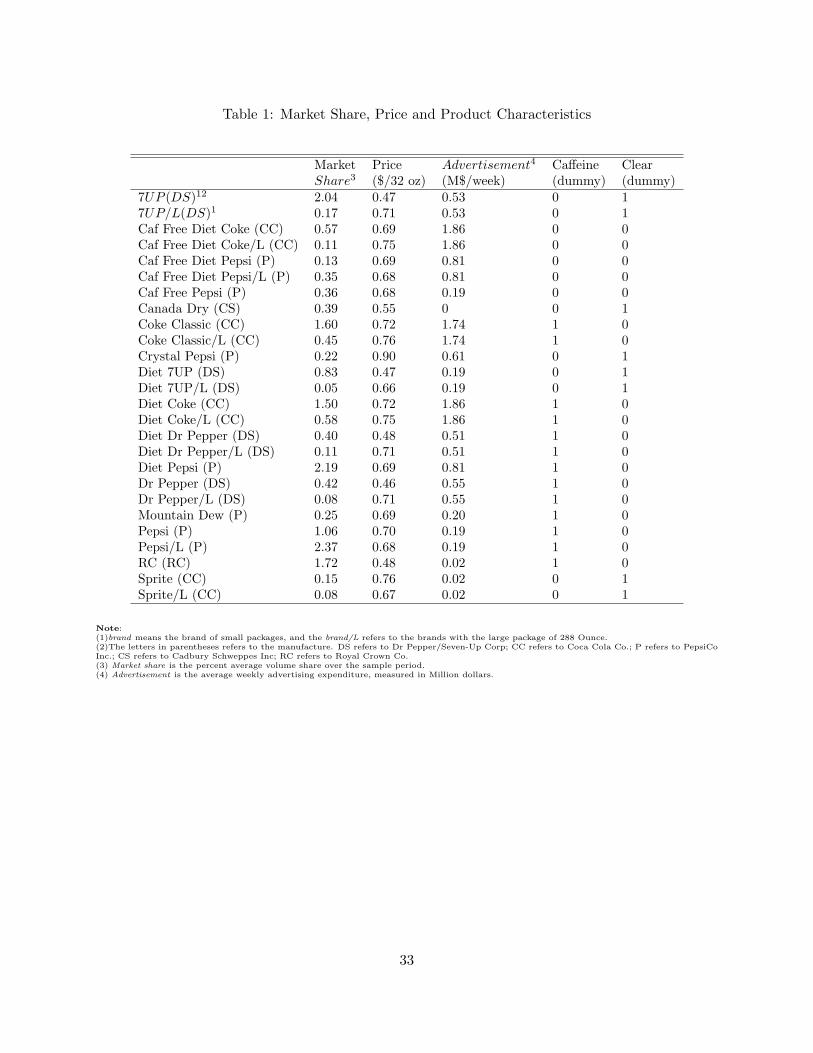
Table 1: Market Share, Price and Product Characteristics

Market Price Advertisement4 Caffeine ClearShare3 ($/32 oz) (M$/week) (dummy) (dummy)

7UP (DS)12 2.04 0.47 0.53 0 17UP/L(DS)1 0.17 0.71 0.53 0 1Caf Free Diet Coke (CC) 0.57 0.69 1.86 0 0Caf Free Diet Coke/L (CC) 0.11 0.75 1.86 0 0Caf Free Diet Pepsi (P) 0.13 0.69 0.81 0 0Caf Free Diet Pepsi/L (P) 0.35 0.68 0.81 0 0Caf Free Pepsi (P) 0.36 0.68 0.19 0 0Canada Dry (CS) 0.39 0.55 0 0 1Coke Classic (CC) 1.60 0.72 1.74 1 0Coke Classic/L (CC) 0.45 0.76 1.74 1 0Crystal Pepsi (P) 0.22 0.90 0.61 0 1Diet 7UP (DS) 0.83 0.47 0.19 0 1Diet 7UP/L (DS) 0.05 0.66 0.19 0 1Diet Coke (CC) 1.50 0.72 1.86 1 0Diet Coke/L (CC) 0.58 0.75 1.86 1 0Diet Dr Pepper (DS) 0.40 0.48 0.51 1 0Diet Dr Pepper/L (DS) 0.11 0.71 0.51 1 0Diet Pepsi (P) 2.19 0.69 0.81 1 0Dr Pepper (DS) 0.42 0.46 0.55 1 0Dr Pepper/L (DS) 0.08 0.71 0.55 1 0Mountain Dew (P) 0.25 0.69 0.20 1 0Pepsi (P) 1.06 0.70 0.19 1 0Pepsi/L (P) 2.37 0.68 0.19 1 0RC (RC) 1.72 0.48 0.02 1 0Sprite (CC) 0.15 0.76 0.02 0 1Sprite/L (CC) 0.08 0.67 0.02 0 1

Note:(1)brand means the brand of small packages, and the brand/L refers to the brands with the large package of 288 Ounce.(2)The letters in parentheses refers to the manufacture. DS refers to Dr Pepper/Seven-Up Corp; CC refers to Coca Cola Co.; P refers to PepsiCoInc.; CS refers to Cadbury Schweppes Inc; RC refers to Royal Crown Co.(3) Market share is the percent average volume share over the sample period.(4) Advertisement is the average weekly advertising expenditure, measured in Million dollars.

33

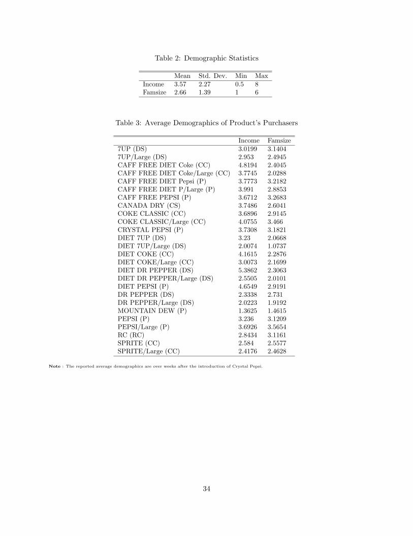
Table 2: Demographic Statistics

Mean Std. Dev. Min MaxIncome 3.57 2.27 0.5 8Famsize 2.66 1.39 1 6

Table 3: Average Demographics of Product’s Purchasers

Income Famsize7UP (DS) 3.0199 3.14047UP/Large (DS) 2.953 2.4945CAFF FREE DIET Coke (CC) 4.8194 2.4045CAFF FREE DIET Coke/Large (CC) 3.7745 2.0288CAFF FREE DIET Pepsi (P) 3.7773 3.2182CAFF FREE DIET P/Large (P) 3.991 2.8853CAFF FREE PEPSI (P) 3.6712 3.2683CANADA DRY (CS) 3.7486 2.6041COKE CLASSIC (CC) 3.6896 2.9145COKE CLASSIC/Large (CC) 4.0755 3.466CRYSTAL PEPSI (P) 3.7308 3.1821DIET 7UP (DS) 3.23 2.0668DIET 7UP/Large (DS) 2.0074 1.0737DIET COKE (CC) 4.1615 2.2876DIET COKE/Large (CC) 3.0073 2.1699DIET DR PEPPER (DS) 5.3862 2.3063DIET DR PEPPER/Large (DS) 2.5505 2.0101DIET PEPSI (P) 4.6549 2.9191DR PEPPER (DS) 2.3338 2.731DR PEPPER/Large (DS) 2.0223 1.9192MOUNTAIN DEW (P) 1.3625 1.4615PEPSI (P) 3.236 3.1209PEPSI/Large (P) 3.6926 3.5654RC (RC) 2.8434 3.1161SPRITE (CC) 2.584 2.5577SPRITE/Large (CC) 2.4176 2.4628

Note : The reported average demographics are over weeks after the introduction of Crystal Pepsi.

34

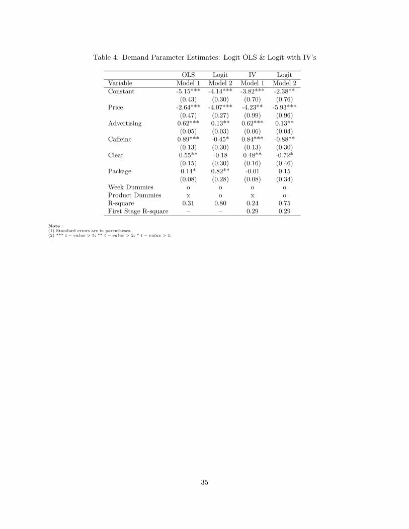
Table 4: Demand Parameter Estimates: Logit OLS & Logit with IV’s

OLS Logit IV LogitVariable Model 1 Model 2 Model 1 Model 2Constant -5.15*** -4.14*** -3.82*** -2.38**

(0.43) (0.30) (0.70) (0.76)Price -2.64*** -4.07*** -4.23** -5.93***

(0.47) (0.27) (0.99) (0.96)Advertising 0.62*** 0.13** 0.62*** 0.13**

(0.05) (0.03) (0.06) (0.04)Caffeine 0.89*** -0.45* 0.84*** -0.88**

(0.13) (0.30) (0.13) (0.30)Clear 0.55** -0.18 0.48** -0.72*

(0.15) (0.30) (0.16) (0.46)Package 0.14* 0.82** -0.01 0.15

(0.08) (0.28) (0.08) (0.34)Week Dummies o o o oProduct Dummies x o x oR-square 0.31 0.80 0.24 0.75First Stage R-square – – 0.29 0.29

Note :(1) Standard errors are in parentheses.(2) *** t − value > 5; ** t − value > 2; * t − value > 1.

35

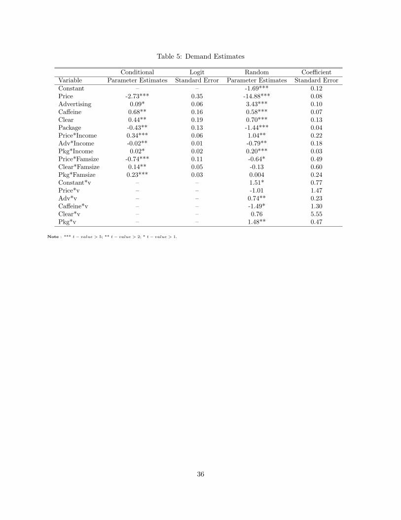
Table 5: Demand Estimates

Conditional Logit Random CoefficientVariable Parameter Estimates Standard Error Parameter Estimates Standard ErrorConstant – – -1.69*** 0.12Price -2.73*** 0.35 -14.88*** 0.08Advertising 0.09* 0.06 3.43*** 0.10Caffeine 0.68** 0.16 0.58*** 0.07Clear 0.44** 0.19 0.70*** 0.13Package -0.43** 0.13 -1.44*** 0.04Price*Income 0.34*** 0.06 1.04** 0.22Adv*Income -0.02** 0.01 -0.79** 0.18Pkg*Income 0.02* 0.02 0.20*** 0.03Price*Famsize -0.74*** 0.11 -0.64* 0.49Clear*Famsize 0.14** 0.05 -0.13 0.60Pkg*Famsize 0.23*** 0.03 0.004 0.24Constant*v – – 1.51* 0.77Price*v – – -1.01 1.47Adv*v – – 0.74** 0.23Caffeine*v – – -1.49* 1.30Clear*v – – 0.76 5.55Pkg*v – – 1.48** 0.47

Note : *** t − value > 5; ** t − value > 2; * t − value > 1.

36

Table 6: Own and Cross-Price Elasticities

Product Canada Coke Crystal DIET Diet Diet Diet Pepsi Pepsi/LDry Classic Pepsi 7UP Coke Coke/L Pepsi

7UP (DS) 0.07 0.17 0.17 0.10 0.13 0.07 0.42 0.16 0.177UP/Large (DS) 0.05 0.05 0.09 0.06 0.06 0.14 0.19 0.07 0.37Caff Free Diet Coke (CC) 0.03 0.37 0.06 0.02 0.36 0.21 0.31 0.03 0.02Caff Free Diet Coke/L (CC) 0.02 0.17 0.04 0.01 0.19 0.40 0.17 0.01 0.02Caff Free Diet Pepsi (P) 0.04 0.34 0.13 0.08 0.21 0.15 0.48 0.16 0.19Caff Free Diet Pepsi/L (P) 0.04 0.12 0.09 0.05 0.09 0.19 0.24 0.10 0.40Caff Free Pepsi (P) 0.03 0.16 0.08 0.08 0.04 0.01 0.31 0.29 0.34Canada Dry (CS) -4.20 0.06 0.12 0.07 0.08 0.06 0.25 0.12 0.14Coke Classic (CC) 0.01 -8.37 0.05 0.03 0.58 0.35 0.74 0.24 0.20Coke Classic/L (CC) 0.01 0.64 0.03 0.03 0.30 0.62 0.52 0.20 0.39Crystal Pepsi (P) 0.06 0.12 -7.36 0.09 0.12 0.05 0.35 0.15 0.16Diet 7UP (DS) 0.07 0.16 0.15 -5.52 0.07 0.03 0.40 0.21 0.24Diet 7UP/L (DS) 0.04 0.03 0.07 0.05 0.03 0.05 0.13 0.07 0.40Diet Coke (CC) 0.02 0.66 0.05 0.02 -7.71 0.40 0.43 0.05 0.04Diet Coke/L (CC) 0.01 0.34 0.02 0.01 0.40 -5.80 0.33 0.02 0.06Diet Dr Pepper (DS) 0.04 0.37 0.07 0.05 0.22 0.14 0.83 0.31 0.37Diet Dr Pepper/L (DS) 0.03 0.10 0.05 0.03 0.09 0.18 0.33 0.15 0.78Diet Pepsi (P) 0.03 0.46 0.07 0.05 0.33 0.22 -7.11 0.28 0.33Dr Pepper (DS) 0.03 0.41 0.07 0.05 0.24 0.16 0.86 0.31 0.36Dr Pepper/L (DS) 0.03 0.11 0.05 0.03 0.09 0.20 0.35 0.16 0.77Mountain Dew (P) 0.05 0.12 0.07 0.04 0.14 0.08 0.57 0.25 0.39Pepsi (P) 0.02 0.24 0.04 0.04 0.06 0.02 0.51 -5.98 0.55Pepsi/Large (P) 0.01 0.07 0.03 0.03 0.01 0.03 0.23 0.24 -3.36RC (RC) 0.06 0.10 0.07 0.04 0.15 0.10 0.54 0.18 0.20Sprite (CC) 0.06 0.10 0.13 0.11 0.05 0.02 0.30 0.22 0.25Sprite/L (CC) 0.04 0.01 0.07 0.04 0.01 0.02 0.07 0.05 0.39

Note :(1) The entry i, j, where i indexes row and j column, gives the percent change in market share of product i with a 1% change in price of j.(2) Each entry is the mean of the elasticities across 26 weeks.

37

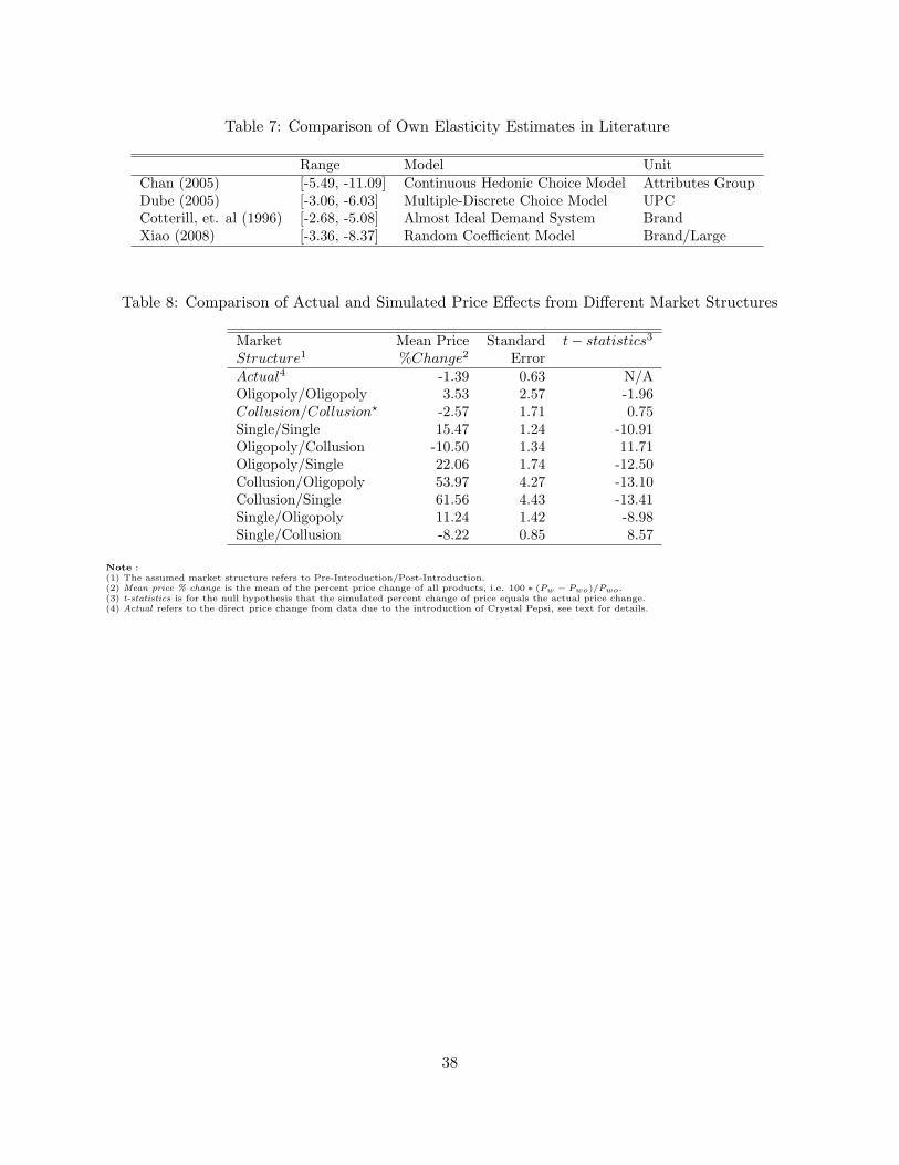
Table 7: Comparison of Own Elasticity Estimates in Literature

Range Model UnitChan (2005) [-5.49, -11.09] Continuous Hedonic Choice Model Attributes GroupDube (2005) [-3.06, -6.03] Multiple-Discrete Choice Model UPCCotterill, et. al (1996) [-2.68, -5.08] Almost Ideal Demand System BrandXiao (2008) [-3.36, -8.37] Random Coefficient Model Brand/Large

Table 8: Comparison of Actual and Simulated Price Effects from Different Market Structures

Market Mean Price Standard t− statistics3

Structure1 %Change2 ErrorActual4 -1.39 0.63 N/AOligopoly/Oligopoly 3.53 2.57 -1.96Collusion/Collusion? -2.57 1.71 0.75Single/Single 15.47 1.24 -10.91Oligopoly/Collusion -10.50 1.34 11.71Oligopoly/Single 22.06 1.74 -12.50Collusion/Oligopoly 53.97 4.27 -13.10Collusion/Single 61.56 4.43 -13.41Single/Oligopoly 11.24 1.42 -8.98Single/Collusion -8.22 0.85 8.57

Note :(1) The assumed market structure refers to Pre-Introduction/Post-Introduction.(2) Mean price % change is the mean of the percent price change of all products, i.e. 100 ∗ (Pw − Pwo)/Pwo.(3) t-statistics is for the null hypothesis that the simulated percent change of price equals the actual price change.(4) Actual refers to the direct price change from data due to the introduction of Crystal Pepsi, see text for details.

38

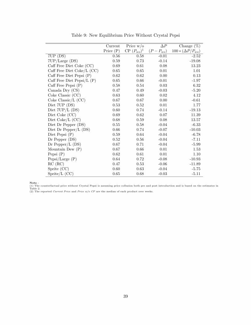
Table 9: New Equilibrium Price Without Crystal Pepsi

Current Price w/o ∆P Change (%)Price (P) CP (Pwo)1 (P − Pwo) 100 ∗ (∆P/Pwo)

7UP (DS) 0.56 0.58 -0.01 -2.527UP/Large (DS) 0.59 0.73 -0.14 -19.08Caff Free Diet Coke (CC) 0.69 0.61 0.08 13.23Caff Free Diet Coke/L (CC) 0.65 0.65 0.01 1.01Caff Free Diet Pepsi (P) 0.62 0.62 0.00 0.13Caff Free Diet Pepsi/L (P) 0.65 0.66 -0.01 -1.97Caff Free Pepsi (P) 0.58 0.54 0.03 6.32Canada Dry (CS) 0.47 0.49 -0.03 -5.20Coke Classic (CC) 0.63 0.60 0.02 4.12Coke Classic/L (CC) 0.67 0.67 0.00 -0.61Diet 7UP (DS) 0.53 0.52 0.01 1.77Diet 7UP/L (DS) 0.60 0.74 -0.14 -19.13Diet Coke (CC) 0.69 0.62 0.07 11.39Diet Coke/L (CC) 0.68 0.59 0.08 13.57Diet Dr Pepper (DS) 0.55 0.58 -0.04 -6.33Diet Dr Pepper/L (DS) 0.66 0.74 -0.07 -10.03Diet Pepsi (P) 0.59 0.64 -0.04 -6.78Dr Pepper (DS) 0.52 0.56 -0.04 -7.11Dr Pepper/L (DS) 0.67 0.71 -0.04 -5.99Mountain Dew (P) 0.67 0.66 0.01 1.53Pepsi (P) 0.62 0.61 0.01 1.10Pepsi/Large (P) 0.64 0.72 -0.08 -10.93RC (RC) 0.47 0.53 -0.06 -11.89Sprite (CC) 0.60 0.63 -0.04 -5.75Sprite/L (CC) 0.65 0.68 -0.03 -5.11

Note :(1) The counterfactual price without Crystal Pepsi is assuming price collusion both pre and post introduction and is based on the estimates inTable 2.(2) The reported Current Price and Price w/o CP are the median of each product over weeks.

39

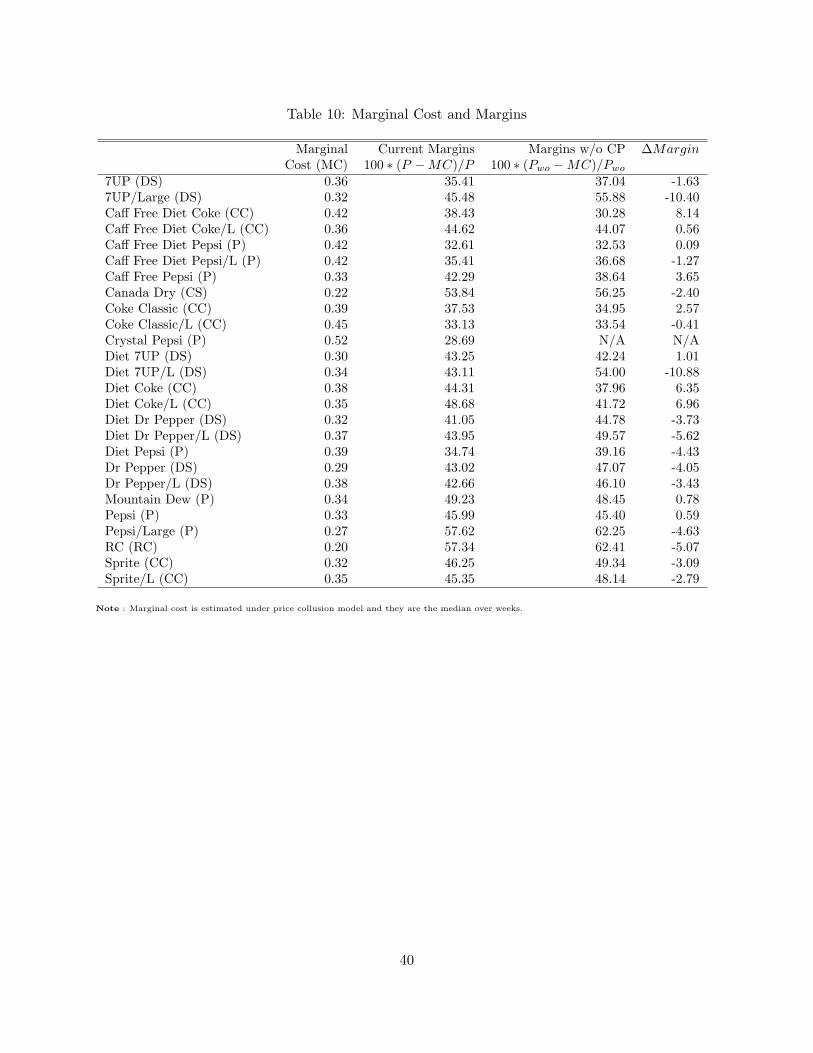
Table 10: Marginal Cost and Margins

Marginal Current Margins Margins w/o CP ∆MarginCost (MC) 100 ∗ (P −MC)/P 100 ∗ (Pwo −MC)/Pwo

7UP (DS) 0.36 35.41 37.04 -1.637UP/Large (DS) 0.32 45.48 55.88 -10.40Caff Free Diet Coke (CC) 0.42 38.43 30.28 8.14Caff Free Diet Coke/L (CC) 0.36 44.62 44.07 0.56Caff Free Diet Pepsi (P) 0.42 32.61 32.53 0.09Caff Free Diet Pepsi/L (P) 0.42 35.41 36.68 -1.27Caff Free Pepsi (P) 0.33 42.29 38.64 3.65Canada Dry (CS) 0.22 53.84 56.25 -2.40Coke Classic (CC) 0.39 37.53 34.95 2.57Coke Classic/L (CC) 0.45 33.13 33.54 -0.41Crystal Pepsi (P) 0.52 28.69 N/A N/ADiet 7UP (DS) 0.30 43.25 42.24 1.01Diet 7UP/L (DS) 0.34 43.11 54.00 -10.88Diet Coke (CC) 0.38 44.31 37.96 6.35Diet Coke/L (CC) 0.35 48.68 41.72 6.96Diet Dr Pepper (DS) 0.32 41.05 44.78 -3.73Diet Dr Pepper/L (DS) 0.37 43.95 49.57 -5.62Diet Pepsi (P) 0.39 34.74 39.16 -4.43Dr Pepper (DS) 0.29 43.02 47.07 -4.05Dr Pepper/L (DS) 0.38 42.66 46.10 -3.43Mountain Dew (P) 0.34 49.23 48.45 0.78Pepsi (P) 0.33 45.99 45.40 0.59Pepsi/Large (P) 0.27 57.62 62.25 -4.63RC (RC) 0.20 57.34 62.41 -5.07Sprite (CC) 0.32 46.25 49.34 -3.09Sprite/L (CC) 0.35 45.35 48.14 -2.79

Note : Marginal cost is estimated under price collusion model and they are the median over weeks.

40

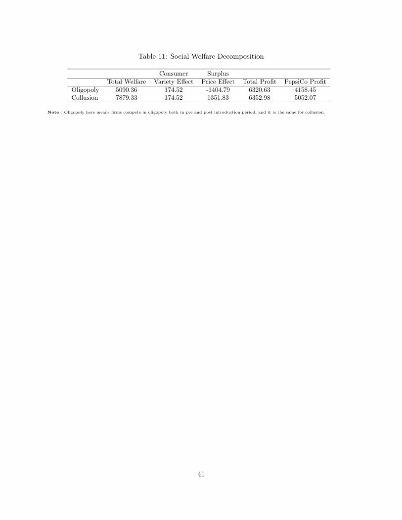
Table 11: Social Welfare Decomposition

Consumer SurplusTotal Welfare Variety Effect Price Effect Total Profit PepsiCo Profit

Oligopoly 5090.36 174.52 -1404.79 6320.63 4158.45Collusion 7879.33 174.52 1351.83 6352.98 5052.07

Note : Oligopoly here means firms compete in oligopoly both in pre and post introduction period, and it is the same for collusion.

41

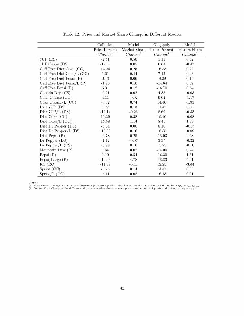
Table 12: Price and Market Share Change in Different Models

Collusion Model Oligopoly ModelPrice Percent Market Share Price Percent Market Share

Change1 Change2 Change1 Change2

7UP (DS) -2.51 0.50 1.15 0.427UP/Large (DS) -19.08 0.05 6.63 -0.47Caff Free Diet Coke (CC) 13.24 0.25 16.53 0.22Caff Free Diet Coke/L (CC) 1.01 0.44 7.43 0.43Caff Free Diet Pepsi (P) 0.13 0.06 -8.29 0.15Caff Free Diet Pepsi/L (P) -1.98 0.16 -14.64 0.32Caff Free Pepsi (P) 6.31 0.12 -16.70 0.54Canada Dry (CS) -5.21 0.02 4.88 -0.03Coke Classic (CC) 4.11 -0.92 9.02 -1.17Coke Classic/L (CC) -0.62 0.74 14.46 -1.93Diet 7UP (DS) 1.77 0.13 11.47 0.00Diet 7UP/L (DS) -19.14 -0.26 8.69 -0.53Diet Coke (CC) 11.39 0.38 19.40 -0.08Diet Coke/L (CC) 13.58 1.14 8.41 1.39Diet Dr Pepper (DS) -6.34 0.00 8.10 -0.17Diet Dr Pepper/L (DS) -10.03 0.16 16.35 -0.09Diet Pepsi (P) -6.78 0.25 -18.03 2.68Dr Pepper (DS) -7.12 -0.07 3.37 -0.22Dr Pepper/L (DS) -5.99 0.16 15.75 -0.10Mountain Dew (P) 1.54 0.02 -14.00 0.24Pepsi (P) 1.10 0.54 -16.30 1.61Pepsi/Large (P) -10.93 4.78 -18.83 4.91RC (RC) -11.89 -0.41 12.25 -3.64Sprite (CC) -5.75 0.14 14.47 0.03Sprite/L (CC) -5.11 0.08 16.73 0.01

Note :(1) Price Percent Change is the percent change of price from pre-introduction to post-introduction period, i.e. 100 ∗ (pw − pwo)/pwo.(2) Market Share Change is the difference of percent market share between post-introduction and pre-introduction, i.e. sw − swo.

42