Incentives for Non-Price Competition in the California WIC Program Job Market … · 2014-10-08 ·...

Incentives for Non-Price Competition in the California WIC

Program

Job Market Paper

Patrick W. McLaughlina,1,2

aDepartment of Agricultural and Resource Economics, University of California, Davis, OneShields Avenue, Davis, California, USA, email: [email protected]

Abstract

Institutional details of the California WIC Program’s food assistance compo-nent give rise to a retailer who does not compete in price for perfectly price inelasticWIC consumers. A theoretical model of non-price competition hypothesizes thatpure non-price competition in brands mimics price competition whereby these re-tailers carry more and better brands under intense spatial competition; and, thatretailers will either minimally or maximally differentiate in horizontal (e.g, physi-cal) space. I use a unique dataset on these retailers’ locations and brand offeringsas well as participants’ food benefit redemption patterns to empirically confirmthat retailers compete in brands. Namely, retailers carry more and better brandsin salient product categories when facing more competitors, which, in turn, re-duces attrition and increases market share. The results also suggest that maximalhorizontal differentiation prevails, allowing the retailers to minimize costly brandcompetition.

1This paper is based on multiple chapters of my dissertation to be completed in 2015 at theUniversity of California, Davis. I express my utmost gratitude to my advisors Richard Sexton,Rachael Goodhue, Tina Saitone and James Chalfant for their guidance and support. Also, Ithank Firas Abu-Sneneh, Matthew Nesvet, Jon Einar Fl̊atnes and participants in the Brown BagSeries in the Department of Agricultural and Resource Economics at University of California,Davis and Selected Presentations at the Agricultural and Applied Economics Association’s 2013Annual Meeting in Washington, D.C. for insightful comments and suggestions.

2This paper is subject to revisions and should not be cited. Please contact the author for thelatest version.

Contents

1 Introduction 3

2 Background 8

3 Previous Work 15

4 Conceptual Framework 194.1 Specific Product Category Incentives . . . . . . . . . . . . . . . . . 194.2 Brand Competition under a Varying Intensity of Spatial Competition 21

5 Data 275.1 In-store Product Survey and Vendor Characteristics . . . . . . . . . 275.2 FI Redemptions . . . . . . . . . . . . . . . . . . . . . . . . . . . . . 305.3 Geographic Location of WIC Vendors . . . . . . . . . . . . . . . . . 345.4 Supermarket Chains Wholesale Costs . . . . . . . . . . . . . . . . . 365.5 Preliminary Descriptive Analysis . . . . . . . . . . . . . . . . . . . 37

6 Empirical Models 446.1 Incentives for Brand Competition . . . . . . . . . . . . . . . . . . . 45

6.1.1 Vendor Attrition . . . . . . . . . . . . . . . . . . . . . . . . 456.1.2 Vendor FI Market Share . . . . . . . . . . . . . . . . . . . . 46

6.2 Non-Price Competition and the Intensity of Spatial Competition . . 476.3 Spatial Error Structure . . . . . . . . . . . . . . . . . . . . . . . . . 50

7 Results 517.1 Incentives for Brand Competition . . . . . . . . . . . . . . . . . . . 52

7.1.1 Vendor Attrition . . . . . . . . . . . . . . . . . . . . . . . . 527.1.2 Vendor FI Market Share . . . . . . . . . . . . . . . . . . . . 557.1.3 Exogeneity of Key Regressors . . . . . . . . . . . . . . . . . 58

7.2 Non-Price Competition and the Intensity of Spatial Competition . . 60

8 Conclusion 61

9 References 65

10 Appendix 70

2

1. Introduction

How will firms compete with one another when they have no incentive to compete

in price? My paper offers an answer to this question using vendors serving the food

assistance component of the California Special Supplemental Nutritional Program

for Women, Infants and Children (California WIC Program) as a case study. The

WIC Program is a federally funded and state administered two-part health inter-

vention and food assistance program for low-income new and to-be mothers, as

well as their infants and young children. The Program is far-reaching nationally,

covering one-half of all newborn infants and one-quarter of all children under the

age of five in the United States (Davis 2007). Over 1.5 million individuals partic-

ipated in the California WIC Program in 2012, accounting for roughly one-sixth

of all participants nationwide.

The institutional details of food assistance in the California WIC Program

render it an ideal yet previously unexplored case study in non-price competition.

First, consumers participating in the Program are insensitive to price due to the

structure of food benefits distribution. The Program provides food benefits to

participants at no cost via redeemable vouchers, or food instruments (FIs), for

fixed quantities of food items of specific product categories. For example, FI

6011 allows for purchase of thirty-six ounces of breakfast cereal, one loaf of whole

wheat bread and one gallon of low-fat milk. Participants can choose any brands

among a Program-approved set, which often includes leading national brands,

when redeeming their FI regardless of the price listed on shelves. In this respect,

WIC differs from other food assistance programs, such as SNAP, where benefits

amount to a direct monetary transfer and participants face budgetary restrictions.

WIC participants, on the other hand, have no incentive to choose inexpensive

3

brands when offered the choice.

My study focuses on the strategic non-price behavior of a subset of retailers

who sell WIC food items. FI redemption takes place at state-authorized WIC

vendors, a diverse group of over 5,500 private retailers in California, as of 2012,

including supercenters (e.g., Walmart), supermarkets (e.g, Safeway), smaller gro-

ceries, corner and convenience stores. WIC vendors provide goods specified by

individual FIs to participants in exchange for reimbursement by the state up to a

pre-specified maximum dollar amount, or maximum allowable departmental reim-

bursement (MADR) in regulation parlance. Vendors record the prices of the goods

sold under the FI to compute the redemption value and have the right to request

reimbursement up to the MADR. Additionally, the Program requires all vendors

to carry at least one brand of every WIC product category, although virtually all

vendors exceed these minimum stocking requirements.

While WIC sales constitute a small fraction of total business for most vendors,

they are the primary source of food business for a special class of vendors, which

are the focus of this study. In particular, roughly one-sixth of all California WIC

vendors are so-called “Above 50%” (A50) vendors, a designation the Program

applies to all vendors with WIC sales comprising 50% or more of all food sales.

A50 vendors are pivotal in the operations of California WIC, accounting for over

one-third of all WIC transactions in the state. Because participants almost exclu-

sively comprise A50 vendors’ food customer base, these vendors have no strategic

incentive to lower the prices charged for WIC items to attract WIC consumers

due to the perfect inelasticity of their demand. In this sense, my study organically

abstracts from price competitive behavior allowing me to observe pure non-price

competition in a market setting.

4

One opportunity for A50 vendors to engage in non-price competition is the

quantity and quality of brands that they carry. California WIC authorizes numer-

ous brands, for which some product categories are highly horizontally (e.g., flavors

of breakfast cereal) and vertically differentiated (e.g., national versus “off” brands).

If WIC participants have strong preferences for particular brands, then A50 ven-

dors have an incentive to craft their WIC brand profile to attract customers. On

the other hand, government payments reimbursing vendors are capped, and carry-

ing more and better brands is costly, thus decreasing margins on FI redemptions.

Hence, it is unclear a priori that A50 vendors will engage in costly non-price

competition, and, if they do, what form it will take.

As the distance between competitors diminishes, or as they become more nu-

merous, A50 vendors’ incentive to strengthen their brand profile increases as a way

to attract and maintain WIC customers. The threat of costly brand competition

may cause vendors to choose retail locations in order to minimize the intensity of

spatial competition. On the other hand, restrictions placed by California WIC on

the eligible set of food items may limit the amount of brand competition that ven-

dors can undertake. In this case, vendors can agglomerate in one location without

having to succumb to brand competitive measures. Thus, the institutional details

of the Program may interact with the strategic behavior of A50 vendors in complex

ways that are little understood presently.

To the above end, I develop a theoretical model of non-price competition where

vendors choose locations in the tradition of Hotelling (1929) and the quality of

brands that they sell. The model is consistent with the idea that the strength

of the optimal brand profile increases with the intensity of spatial competition.

In general, whether A50 vendors adhere to a principle of minimal or maximal

5

horizontal differentiation depends upon the strength of the cost restrictions. I

show that both strategies are Nash equilibiria and develop an empirical approach

to uncover which equilibrium persists in a real market setting. The addition of

space distinguishes my study from previous work on non-price competition in the

airline industry (Douglas and Miller 1974; White 1972) and causes me to arrive at

more nuanced conclusions.

I empirically examine the incentives of A50 vendors to engage in brand compe-

tition using a unique cross-sectional data source on the location and characteristics

of WIC vendors and the redemption patterns of participants. In particular, I ob-

serve the brand profile and in-store characteristics of a random sample of A50

vendors; and for all WIC vendors, their geographic location and the FIs redeemed

over multiple years with a unique participant identification number. I use the

location of WIC vendors to define two variables measuring the intensity of spatial

competition that an A50 vendor faces.

First, I find that having more of certain brand types reduces vendor attri-

tion, the rate at which participants fail to be repeat customers. Contrary to the

common belief that food assistance-eligible consumers face limited food retail op-

tions, I observe that a significant number of participants commit vendor attrition

when the proximity of other A50 competitors grows. In such an environment,

A50 vendors with more of certain brand types (but not others) experience less

attrition, effectively minimizing the intensity of spatial competition. Therefore,

one demonstrated incentive for brand competition is to relieve the competitive

pressure applied by nearby rival vendors.

Second, I find that vendors who carry more numerous and costly brands of cer-

tain product categories have higher benefit redemption market shares, a necessary

6

condition for the profitability of brand competition. Brand variables positively

relate to market share for only a subset of product categories, which is consistent

with the first set of findings. Vendors with more and better brands of breakfast ce-

real claim a higher market share of FI redemptions, a result not replicated for fruit

juice brands. These results reflect the brand offerings of A50 vendors: many high-

cost, leading brands of breakfast cereal are available on nearly all A50 vendors’

shelves, however the offering of juice brands is much more heterogeneous in this

regard. It appears then that A50 vendors may optimally focus brand competition

in specific categories rather than improve variety overall when they cannot strate-

gically set prices. Additionally, policymakers looking to reduce Program costs can

disallow expensive brands that consumers care little about without significantly

impacting welfare.

Last, I empirically model the average wholesale costs of vendors’ brand profiles,

a proxy for quality, as a function of the intensity of spatial competition. This

approach allows me to test the prediction that more spatial competition leads to

increased brand competition while assessing whether vendors tend to minimally

or maximally differentiate. Accounting for the theorized endogeneity and spatial

autocorrelation in the errors, I confirm that A50 vendors carry more and better

brands when they face more competitors. Further, results from estimation are

consistent with vendors maximally but not minimally horizontally differentiating,

on average (Hotelling 1929; d’Aspremont et al. 1979). I find then that non-

price competition is analogous to price competition where firms seek out mutually

disparate locations to alleviate the competitive pressures they place on one other.

Further, the degree of allowed brand competition enhances access to the California

WIC Program by indirectly encouraging more A50 vendor locations compared to

7

a case where expensive and preferred brands are disallowed. This finding suggests

that the competitive structure of WIC FI redemptions can alleviate problems of

food access and food deserts.

The contribution of my work to the economics literature is twofold. First, my

paper characterizes non-price competition in a context where price competition

is irrelevant. My findings differ from previous applications studying non-price

competition in several key ways. Second, my work relates the implications of non-

price competition to the operations and efficiency to the California WIC Program,

a contribution no other study has made to date. In particular, realized non-price

competition bears implications for cost-saving measures related to food benefits

provision and increased food access in the California WIC Program.

The organization of my paper is as follows. I provide detailed background on

the California WIC program in the immediately proceeding section to motivate

the incentives vendor and participants face. The next section places my work

in the literature. The conceptual framework follows, including a description of

the incentives to invest in brand competition in specific product categories and a

theoretical model of brand and spatial competition. Then, I describe the vendor

survey, participant benefits redemptions and in-store and geographical data in

the subsequent section. Then, I provide a preliminary descriptive analysis of the

competitive environment and brand profile of A50 vendors to motivate hypotheses.

I present three empirical models to test these hypotheses and discuss the results

of their estimation. The final section concludes.

2. Background

The federal government funds all WIC Programs and charges states with admin-

istering the provision of supplemental food, nutritional counseling, and access to

8

health-care services. Eligible participant candidates have a household income of at

most 185% of the federal poverty line and are often eligible for or receiving Supple-

mental Nutrition Assistance Program (SNAP; formerly known as Food Stamps),

Temporary Assistance for Needy Families (TANF) and/or Medicaid benefits. Par-

ticipants receive food assistance benefits and other health care and educational

resources at local WIC clinics.

State WIC programs provide the supplemental food to the participant at no

cost and are responsible for reimbursing state authorized WIC food vendors. The

federal government mandates product categories that are beneficial to the well-

being of prenatal and postpartum mothers and the healthy development of their

newborns and young children.3 However, it is the responsibility of the individual

state to approve specific food brands, package sizes, and types from which WIC

participants are allowed to choose (USDA FNS 2013).

The California WIC Program’s criteria for authorizing a food item include

that a given food brand or type (a) promotes (or at a minimum, does not detract

from) WIC health and nutrition goals, while being a product that participants

would want to consume and (b) helps maintain the cost-effectiveness of the Pro-

gram, while being consistently available on the wholesale market (California DPH

2012a).4 Product categories require either brand specific or non-brand specific

approval. For example, the Program subjects individual brands of ready-to-eat

breakfast cereal to the approval process but generally allows all brands of oatmeal

3The mandated product categories include infant formula and infant foods, milk, eggs, cheese,dry beans and lentils, peanut butter, breakfast cereal, fruit juice, and whole grain products.

4The approval process for infant formula, on the other hand, is unique compared to all otherproduct categories. The California WIC Program approves a single brand of infant formula byway of a bidding process that selects the manufacturer who offers the highest per unit rebateto the state agency following reimbursement of the WIC vendors (USDA FNS 2013, CaliforniaDPH 2012a).

9

provided they have no feature at odds with approval criteria.5 In practice, the

requirements allow vendors to stock and participants to purchase multiple brands

of most product categories to varying degrees.

The latter criterion of cost-effectiveness ensures that candidate food brands and

types are not so costly that they could undermine the ability of WIC to adequately

provide benefits. Because WIC is not an entitlement program it must maximize

Program benefits under a fixed annual budget constraint, necessitating the re-

quirement for cost control. In California, the Program administration minimizes

costs in the non-brand-specific approval process by excluding product types that

are premium, luxury or otherwise highly priced compared to related goods.6 Nev-

ertheless, the cost of brands eligible for FI redemption varies considerably within

and across product categories.

Program participants “purchase” the supplementary food by means of re-

deemable food vouchers, or food instruments (FIs), for specified bundles of WIC-

approved products. Consumers receive FIs monthly for bundles that vary in

breadth from a month’s supply of infant formula to a basket of low-fat milk, eggs,

cheese, and peanut butter or dry beans. Table 1 describes the top five leading FIs

of the California WIC Program in terms of the number redeemed and dollar value.

The top three FIs are combination food packages that allow for multiple product

categories for purchase. The fourth and fifth leading FIs provide multiple quanti-

ties of infant formula for which only one specific brand is approved for purchase

5For example, oatmeal labeled as organic or produced with added sugar is not eligible forpurchase.

6For example, the state agency approves many types of cheese (e.g., cheddar) where any brandis permissible; however all brands of more expensive artisan or organic cheeses are excluded(California DPH 2012). For brand-specific product categories, certain brands may not receiveapproval if they are prohibitively costly even if they meet nutritional requirements, (e.g., organiccold breakfast cereals) (California DPH 2012).

10

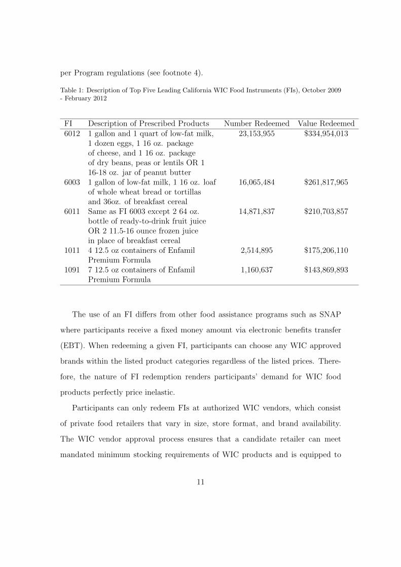
per Program regulations (see footnote 4).

Table 1: Description of Top Five Leading California WIC Food Instruments (FIs), October 2009- February 2012

FI Description of Prescribed Products Number Redeemed Value Redeemed6012 1 gallon and 1 quart of low-fat milk, 23,153,955 $334,954,013

1 dozen eggs, 1 16 oz. packageof cheese, and 1 16 oz. packageof dry beans, peas or lentils OR 116-18 oz. jar of peanut butter

6003 1 gallon of low-fat milk, 1 16 oz. loaf 16,065,484 $261,817,965of whole wheat bread or tortillasand 36oz. of breakfast cereal

6011 Same as FI 6003 except 2 64 oz. 14,871,837 $210,703,857bottle of ready-to-drink fruit juiceOR 2 11.5-16 ounce frozen juicein place of breakfast cereal

1011 4 12.5 oz containers of Enfamil 2,514,895 $175,206,110Premium Formula

1091 7 12.5 oz containers of Enfamil 1,160,637 $143,869,893Premium Formula

The use of an FI differs from other food assistance programs such as SNAP

where participants receive a fixed money amount via electronic benefits transfer

(EBT). When redeeming a given FI, participants can choose any WIC approved

brands within the listed product categories regardless of the listed prices. There-

fore, the nature of FI redemption renders participants’ demand for WIC food

products perfectly price inelastic.

Participants can only redeem FIs at authorized WIC vendors, which consist

of private food retailers that vary in size, store format, and brand availability.

The WIC vendor approval process ensures that a candidate retailer can meet

mandated minimum stocking requirements of WIC products and is equipped to

11

handle FI redemptions (USDA FNS 2013). The minimum stocking requirements

amount to vendors maintaining an inventory such that at least one brand of each

product category is available for purchase at all times. As later revealed in the

data, virtually all WIC vendors exceed the minimum stocking requirements in all

product categories. For most vendors, many non-WIC customers also purchase the

WIC goods and hence the minimum requirements are likely irrelevant. However,

for vendors with a large number of WIC customers and an effectively fixed FI

reimbursement payment, the only incentive to carry more and better brands is to

compete with other vendors.

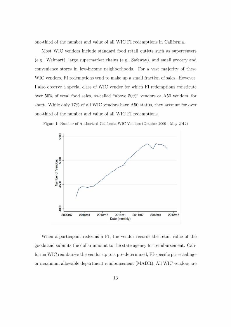
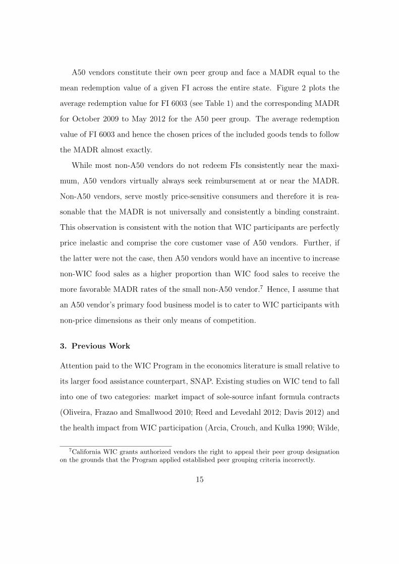
There are many WIC vendors in California, presently amounting to over 5,500

food retailers. Figure 1 depicts the number of vendors from October 2009 to

May 2012. For most of this time frame, a significant amount of entry occurred,

suggesting food retailers see WIC authorization as highly lucrative. The number of

WIC vendors leveled off toward the end of 2011, however, as result of a USDA Food

and Nutrition Service (FNS) moratorium on new vendor authorization imposed

that same year (California DPH 2012b). This number remained stable throughout

the early part of 2012, the time period of the in-store product survey that informs

the quantity and quality of brands for this study.

WIC vendors include standard food retail outlets such as supercenters (e.g.,

Walmart), large supermarket chains (e.g., Safeway), and small grocery and con-

venience stores in low-income neighborhoods. For a vast majority of these WIC

vendors, FI redemptions tend to make up a small fraction of total sales. However,

I also observe a special class of WIC vendor for which FI redemptions constitute

over 50% of total food sales, so-called “above 50%” vendors or A50 vendors, for

short. While only 17% of all WIC vendors have A50 status, they account for over

12

one-third of the number and value of all WIC FI redemptions in California.

Most WIC vendors include standard food retail outlets such as supercenters

(e.g., Walmart), large supermarket chains (e.g., Safeway), and small grocery and

convenience stores in low-income neighborhoods. For a vast majority of these

WIC vendors, FI redemptions tend to make up a small fraction of sales. However,

I also observe a special class of WIC vendor for which FI redemptions constitute

over 50% of total food sales, so-called “above 50%” vendors or A50 vendors, for

short. While only 17% of all WIC vendors have A50 status, they account for over

one-third of the number and value of all WIC FI redemptions.

Figure 1: Number of Authorized California WIC Vendors (October 2009 - May 2012)

When a participant redeems a FI, the vendor records the retail value of the

goods and submits the dollar amount to the state agency for reimbursement. Cali-

fornia WIC reimburses the vendor up to a pre-determined, FI-specific price ceiling–

or maximum allowable department reimbursement (MADR). All WIC vendors are

13

aware of the various MADRs they face, which the Program updates on a biweekly

basis. The purpose of the MADR is to control costs by preventing WIC vendors

from setting exceedingly high prices for goods purchased by price-unresponsive

participants.

The MADR of a given FI varies by peer group, a grouping of vendors defined by

store size as measured by number of check-out registers, geographical region and

A50 status. Prior to the end of May 2012, California WIC computed the MADR

as a twelve-week rolling average of the FI redemption values of a given non-A50

peer group plus a group-specific tolerance factor dependent upon redemption value

variance. Presently, new California WIC regulations specify that small vendors

with one or two registers (three or four registers) have a MADR of a 15% (11%)

markup over the average redemption value of large non-A50 vendors, although

data presented in this study do not reflect this change.

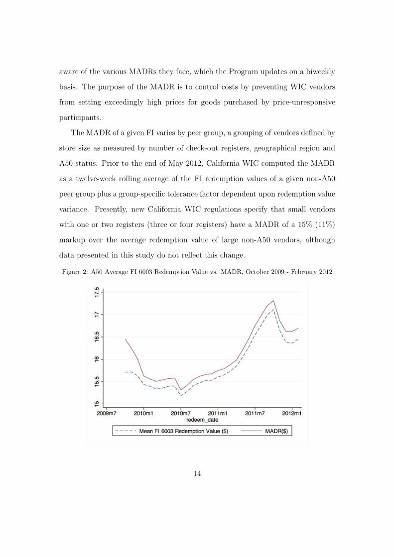
Figure 2: A50 Average FI 6003 Redemption Value vs. MADR, October 2009 - February 2012

14

A50 vendors constitute their own peer group and face a MADR equal to the

mean redemption value of a given FI across the entire state. Figure 2 plots the

average redemption value for FI 6003 (see Table 1) and the corresponding MADR

for October 2009 to May 2012 for the A50 peer group. The average redemption

value of FI 6003 and hence the chosen prices of the included goods tends to follow

the MADR almost exactly.

While most non-A50 vendors do not redeem FIs consistently near the maxi-

mum, A50 vendors virtually always seek reimbursement at or near the MADR.

Non-A50 vendors, serve mostly price-sensitive consumers and therefore it is rea-

sonable that the MADR is not universally and consistently a binding constraint.

This observation is consistent with the notion that WIC participants are perfectly

price inelastic and comprise the core customer vase of A50 vendors. Further, if

the latter were not the case, then A50 vendors would have an incentive to increase

non-WIC food sales as a higher proportion than WIC food sales to receive the

more favorable MADR rates of the small non-A50 vendor.7 Hence, I assume that

an A50 vendor’s primary food business model is to cater to WIC participants with

non-price dimensions as their only means of competition.

3. Previous Work

Attention paid to the WIC Program in the economics literature is small relative to

its larger food assistance counterpart, SNAP. Existing studies on WIC tend to fall

into one of two categories: market impact of sole-source infant formula contracts

(Oliveira, Frazao and Smallwood 2010; Reed and Levedahl 2012; Davis 2012) and

the health impact from WIC participation (Arcia, Crouch, and Kulka 1990; Wilde,

7California WIC grants authorized vendors the right to appeal their peer group designationon the grounds that the Program applied established peer grouping criteria incorrectly.

15

McNamara, and Ranney 1999; Carlson and Senauer 2003). My work departs from

both categories by using the WIC program to answer broader questions of non-price

competition relevant to food retail, industrial organization, and efficient operation

of the WIC Program.

There is a longstanding general interest in the economics of non-price com-

petition. One classic application is in the United States’ airline industry where

price was effectively parametric to firms prior to deregulation (Douglas and Miller

1974). The bulk of the literature examines the incentives to compete in advertising

(Stigler 1968) and quality as measured by the frequency of flights (Douglas and

Miller 1974; White 1972). These authors conclude that (a) non-price dimensions

are determined by the level of a fixed price and (b) that costly non-price com-

petition can eliminate rents despite a small number of firms and no free entry.

For example, Douglas and Miller (1974) theorize that airlines offer more frequent

flights, reducing the distance of scheduled flights to consumers’ ideally preferred

times, until profits are exhausted. My context differs from the regulated airline

example in two key ways: one, WIC consumers are perfectly price inelastic and

hence all price considerations are abstracted from; and, two, the added component

of differentiation in physical space gives the opportunity for firms to earn positive

rents.

Non-price competition and spatial competition have also long been studied to-

gether by economists. In a model of horizontal differentiation, Hotelling (1929) first

argued for the principle of minimum differentiation where two profit-maximizing

firms choose identical central locations along a segmented line generally inter-

pretable as firm characteristic space.8 Later, d’Aspremont et al. (1979) proved

8A horizontally differentiated attribute is one where no value of the attribute ranks higher

16

that firms instead optimally locate on the end point of the line for some model

specifications–or the principle of maximum differentiation. Price-setting firms op-

timally choose their non-price attributes to limit head-to-head competition, max-

imizing distance from the competitor to lessen price competition. On the other

hand, Hotelling’s result is valid under non-price competition (i.e., if prices are

fixed). While the space of “more and better” brands is not horizontal per se, I

use this context of the theoretical literature to ask: will firms use their non-price

characteristics to distance themselves from competitors even when they do not

strategically set prices?

One possibility is that firms will compete in some dimensions but not others.

Work generalizing the Hotelling (1929) framework to multiple dimensions finds a

mixture of evidence for both the principles of minimum and maximum differenti-

ation. For two or more dimensions, Tabuchi (1994) and Irmen and Thisse (1998)

show that two firms will maximally differentiate in one dimension and minimally

differentiate in the other(s). In particular, firms maximally differentiate in dimen-

sions where there is the greatest opportunity (i.e., the line is the longest) and

the transportation costs in utility terms are the highest. On the other hand, de

Palma et al. (1985) show that the principle of minimum differentiation holds in

all dimensions when consumers view firms as significantly heterogeneous in some

exogenous characteristic. Again, the brand variables are not strictly horizontal;

however this literature frames the question of whether non-price competitive firms

will choose to compete in all brand or product characteristics, or only a select few

to minimize the intensity of spatial competition.

than any other per se in utility term; and consumers have their own ideal preferred value of theattribute (i.e., an address). Examples include different flavors of breakfast cereal or fruit juiceand their literal geographic location.

17

Alternative characterizations of brand competition include the non-address ap-

proach to variety competition of Dixit and Stiglitz (1977) and Spence (1976); and

the vertical differentiation models of Mussa and Rosen (1978) and Shaked and

Sutton (1982). For example, Dixit and Stiglitz (1977) discuss the ambiguity of

competitive equilibria producing optimal product variety; however, if two product

categories have similar costs, firms will specialize in a product category with a

low elasticity of substitution. Shaked and Sutton (1982) characterize oligopolis-

tic competition in vertical differentiation where only firms producing high quality

(e.g., carrying more expensive brands) earn positive profits. My work evaluates

such predictions in a natural food retail setting where firms do not compete in

price.

Second, my work complements the existing empirical literature on non-price

competition in food retail. A consistent finding of existing studies is that compet-

ing in non-price dimensions can help maintain a relatively price-inelastic customer

base, allowing retailers to charge higher prices. For example, Bonanno and Lopez

(2009) find that supermarkets tend to increase milk prices to capture consumer

surplus when they offer both additional food and non-food services. Richards and

Hamilton (2006) find that price and variety of fresh fruit offerings are strategic

complements with consumers’ higher willingness to pay. However, the response

in variety alone across competing supermarkets is heterogeneous, where variety of

one firm responds to some competitors but not others. Matsa (2011) shows that

supermarkets under intense spatial competition increase the quality of their stores

via reducing the frequency that carried products “stock-out”, a result amplified by

the presence highly price-competitive Walmart. To the extent that the confound-

ing presence of price competition drives any of the preceding results, my work

18

characterizes some of the incentives food retailers have to compete in non-price

attributes alone.

4. Conceptual Framework

I present the conceptual foundation of my study in two parts. In each, I assume

that the primary function of the A50 vendor is to “sell” FI redemptions, where WIC

consumer demand for FI redemptions at a particular vendor is a function of offered

brands and location. Given the incentive to compete in non-price dimensions, the

first part discusses the incentives to invest in brands of some product categories but

not others when optimally choosing the non-price attribute. This section provides

an overview of general hypotheses of how A50 vendors respond to the institutional

details of the California WIC Program as well as consumer demand for WIC food

products. I present a framework where A50 vendors may compete in brands of

some product categories but not others.

The second part spells out the incentives to offer more and better brands of

WIC goods under intense spatial competition, and characterizes how vendors will

locate under such competition. In particular, I revise the analysis of Hotelling

(1929) to a setting where price is exogenously fixed and vendors strategically choose

a non-price attribute instead. I find that A50 vendors carry more and better brands

the closer they are to one another; and, multiple equilibria in strategically chosen

geographic location exist.

4.1. Specific Product Category Incentives

A combination of the structure of FIs, the set of goods eligible for redemption

and characteristics of consumer demand likely determine the product categories in

which A50 vendors will compete. First, consider the FIs themselves, for example

19

FIs 6003 and 6011, the second and third leading FIs in terms of redemption number

and dollar value. FI 6003 allows for one gallon of low-fat milk, one sixteen-ounce

loaf of whole wheat bread and thirty-six ounces of breakfast cereal; and FI 6011,

which offers the same as FI 6003 except for two sixty-four ounce bottles of fruit

juice in place of the breakfast cereal. Participants can purchase, for instance, three

12-ounce boxes or one 36-ounce box under FI 6003; or, redeem two 64-ounce bottles

of juice under FI 6011. Vendors may carry multiple brands from these product

categories to capitalize on a preference for variety in these product categories if

one exists. On the other hand, both of these two FIs allow only one whole-wheat

bread purchase, eliminating an incentive to stock multiple brands due to variety

preferences.

Vendors may also stock many brands of a highly horizontally differentiated

product category regardless of any preference for variety. For example, consider

brands of breakfast cereal, a classic and broadly horizontally differentiated good.

If different subsets of participants prefer specific brands of breakfast cereal over

all other brands on the basis of horizontal attributes then vendors may do well to

stock many. As the number of breakfast cereal brands increases, the vendor be-

comes closer to each group of participant in product space, increasingly obtaining

participants’ patronage. However, for relatively homogenous product categories

(e.g., low-fat milk) the breadth of horizontal differentiation is limited. Hence, a

small number of brands likely will persist for these categories.

Variation in the restrictiveness of WIC product eligibility categories may result

in brands proliferating for some types but not others. For example, WIC allows

for many different breakfast cereals brands with various grain contents and hence

flavors. On the other hand, WIC explicitly limits eligible bread to “100% whole

20

wheat” loaves with very limited added ingredients. Other cost-reduction-inspired

restrictions such as no organic whole wheat bread reduces the set of available

bread brands on the quality dimension as well. Hence, the types of bread A50

vendors can stock may be relatively homogenous, incentivizing vendors to stock

few brands and seek out the cheapest ones. However, there are comparatively

large sets of nationally recognizable as well as less prolific “off-brands” of breakfast

cereal and fruit juice brands from which A50 vendors can choose, and hence more

opportunities for brand competition.

Even though breakfast cereal and fruit juice vary considerably in terms of hor-

izontal characteristics and potential quality, ultimately the strength of consumer

demand for specific brands will impact A50 vendors’ chosen brand profile. In the

case of breakfast cereal, studies find that high price-cost margins come mainly from

consumers’ high willingness to pay for their most preferred brand (Nevo 2001) to

which consumers exhibit strong loyalty (Chidmi and Lopez 2007). This strong

preference for specific brands likely carries over to price-inelastic FI redemptions.

Consumers in the fruit juice market, on the other hand, do not exhibit strong con-

sumer preferences for brands. For example, Huang, Perloff and Villas-Boas (2006)

observe that orange juice consumers are highly sensitive to price and frequently

substitute across different brands. Thus having more and better brands in this

product category is less likely to have an impact on the number of FIs that a

vendor redeems. A50 vendors then may do well to invest in more preferred yet

expensive breakfast cereal brands rather than the costly juice ones.

4.2. Brand Competition under a Varying Intensity of Spatial Competition

The following models the optimal combination of chosen brands and location

among A50 vendors facing pure non-price competition. I assume WIC participants

21

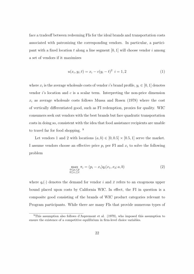
face a tradeoff between redeeming FIs for the ideal brands and transportation costs

associated with patronizing the corresponding vendors. In particular, a partici-

pant with a fixed location t along a line segment [0, 1] will choose vendor i among

a set of vendors if it maximizes

u(xi, yi; t) = xi − c(yi − t)2 i = 1, 2 (1)

where xi is the average wholesale costs of vendor i’s brand profile, yi ∈ [0, 1] denotes

vendor i’s location and c is a scalar term. Interpreting the non-price dimension

xi as average wholesale costs follows Mussa and Rosen (1978) where the cost

of vertically differentiated good, such as FI redemption, proxies for quality. WIC

consumers seek out vendors with the best brands but face quadratic transportation

costs in doing so, consistent with the idea that food assistance recipients are unable

to travel far for food shopping. 9

Let vendors 1 and 2 with locations (a, b) ∈ [0, 0.5] × [0.5, 1] serve the market.

I assume vendors choose an effective price pi per FI and xi to solve the following

problem

max0≤pi≤p̄0≤xi≤x̄

πi = (pi − xi)qi(x1, x2; a, b) (2)

where qi(·) denotes the demand for vendor i and x̄ refers to an exogenous upper

bound placed upon costs by California WIC. In effect, the FI in question is a

composite good consisting of the brands of WIC product categories relevant to

Program participants. While there are many FIs that provide numerous types of

9This assumption also follows d’Aspremont et al. (1979), who imposed this assumption toensure the existence of a competitive equilibrium in firm-level choice variables.

22

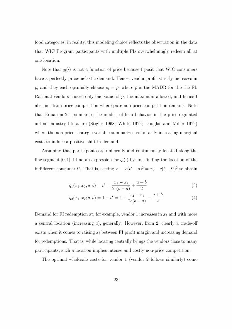
food categories, in reality, this modeling choice reflects the observation in the data

that WIC Program participants with multiple FIs overwhelmingly redeem all at

one location.

Note that qi(·) is not a function of price because I posit that WIC consumers

have a perfectly price-inelastic demand. Hence, vendor profit strictly increases in

pi and they each optimally choose pi = p̄, where p̄ is the MADR for the the FI.

Rational vendors choose only one value of p, the maximum allowed, and hence I

abstract from price competition where pure non-price competition remains. Note

that Equation 2 is similar to the models of firm behavior in the price-regulated

airline industry literature (Stigler 1968; White 1972; Douglas and Miller 1972)

where the non-price strategic variable summarizes voluntarily increasing marginal

costs to induce a positive shift in demand.

Assuming that participants are uniformly and continuously located along the

line segment [0, 1], I find an expression for qi(·) by first finding the location of the

indifferent consumer t?. That is, setting x1− c(t?− a)2 = x2− c(b− t?)2 to obtain

q1(x1, x2; a, b) = t? =x1 − x2

2c(b− a)+a+ b

2(3)

q2(x1, x2; a, b) = 1− t? = 1 +x2 − x1

2c(b− a)− a+ b

2(4)

Demand for FI redemption at, for example, vendor 1 increases in x1 and with more

a central location (increasing a), generally. However, from 2, clearly a trade-off

exists when it comes to raising xi between FI profit margin and increasing demand

for redemptions. That is, while locating centrally brings the vendors close to many

participants, such a location implies intense and costly non-price competition.

The optimal wholesale costs for vendor 1 (vendor 2 follows similarly) come

23

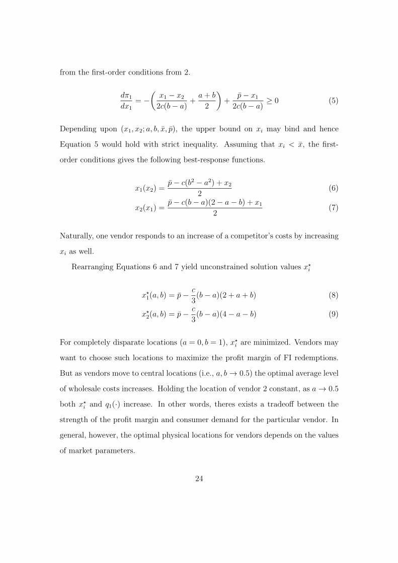
from the first-order conditions from 2.

dπ1

dx1

= −(x1 − x2

2c(b− a)+a+ b

2

)+

p̄− x1

2c(b− a)≥ 0 (5)

Depending upon (x1, x2; a, b, x̄, p̄), the upper bound on xi may bind and hence

Equation 5 would hold with strict inequality. Assuming that xi < x̄, the first-

order conditions gives the following best-response functions.

x1(x2) =p̄− c(b2 − a2) + x2

2(6)

x2(x1) =p̄− c(b− a)(2− a− b) + x1

2(7)

Naturally, one vendor responds to an increase of a competitor’s costs by increasing

xi as well.

Rearranging Equations 6 and 7 yield unconstrained solution values x?i

x?1(a, b) = p̄− c

3(b− a)(2 + a+ b) (8)

x?2(a, b) = p̄− c

3(b− a)(4− a− b) (9)

For completely disparate locations (a = 0, b = 1), x?i are minimized. Vendors may

want to choose such locations to maximize the profit margin of FI redemptions.

But as vendors move to central locations (i.e., a, b→ 0.5) the optimal average level

of wholesale costs increases. Holding the location of vendor 2 constant, as a→ 0.5

both x?i and q1(·) increase. In other words, theres exists a tradeoff between the

strength of the profit margin and consumer demand for the particular vendor. In

general, however, the optimal physical locations for vendors depends on the values

of market parameters.

24

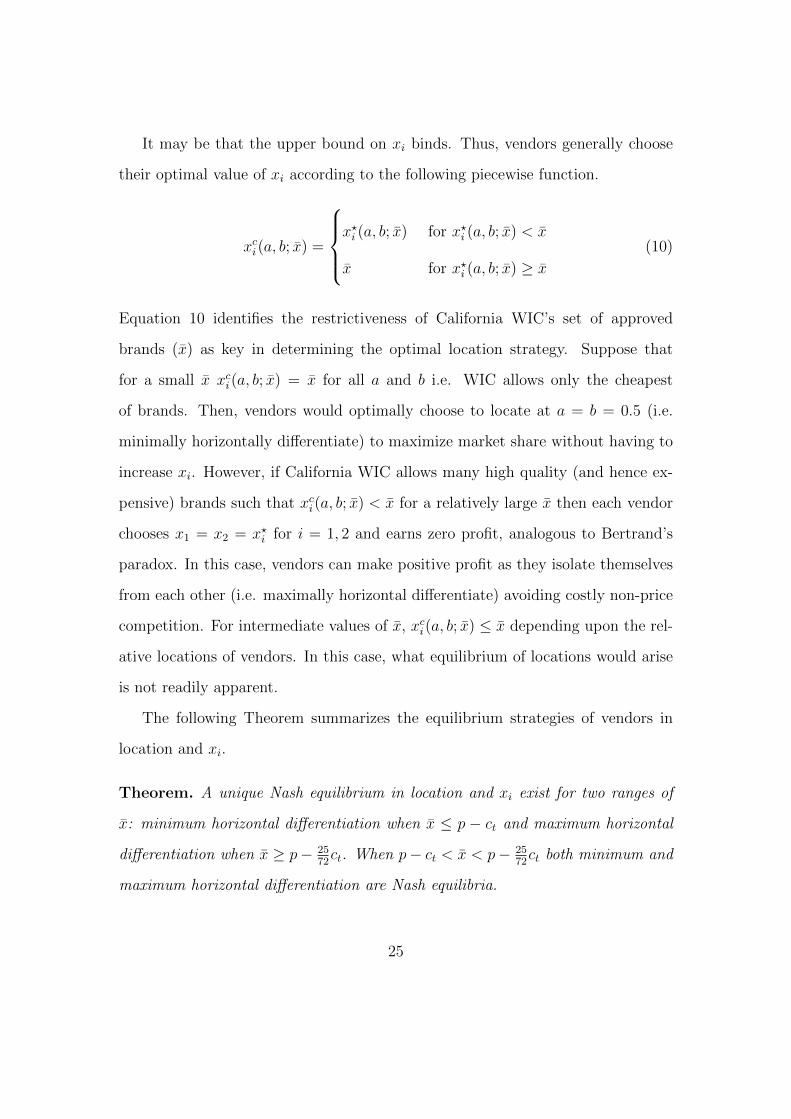
It may be that the upper bound on xi binds. Thus, vendors generally choose

their optimal value of xi according to the following piecewise function.

xci(a, b; x̄) =

x?i (a, b; x̄) for x?i (a, b; x̄) < x̄

x̄ for x?i (a, b; x̄) ≥ x̄

(10)

Equation 10 identifies the restrictiveness of California WIC’s set of approved

brands (x̄) as key in determining the optimal location strategy. Suppose that

for a small x̄ xci(a, b; x̄) = x̄ for all a and b i.e. WIC allows only the cheapest

of brands. Then, vendors would optimally choose to locate at a = b = 0.5 (i.e.

minimally horizontally differentiate) to maximize market share without having to

increase xi. However, if California WIC allows many high quality (and hence ex-

pensive) brands such that xci(a, b; x̄) < x̄ for a relatively large x̄ then each vendor

chooses x1 = x2 = x?i for i = 1, 2 and earns zero profit, analogous to Bertrand’s

paradox. In this case, vendors can make positive profit as they isolate themselves

from each other (i.e. maximally horizontal differentiate) avoiding costly non-price

competition. For intermediate values of x̄, xci(a, b; x̄) ≤ x̄ depending upon the rel-

ative locations of vendors. In this case, what equilibrium of locations would arise

is not readily apparent.

The following Theorem summarizes the equilibrium strategies of vendors in

location and xi.

Theorem. A unique Nash equilibrium in location and xi exist for two ranges of

x̄: minimum horizontal differentiation when x̄ ≤ p − ct and maximum horizontal

differentiation when x̄ ≥ p− 2572ct. When p− ct < x̄ < p− 25

72ct both minimum and

maximum horizontal differentiation are Nash equilibria.

25

Proof. See Appendix.

For the intermediate values of x̄ both minimal and maximal horizontal dif-

ferentiation are optimal strategies. When both vendors choose central locations,

each optimally chooses the maximum quality allowed (xi = x̄) and earns positive

profits. If, say, vendor 1 deviates and locates as far away as possible (a = 0) then

this vendor’s market share falls dramatically relative to their chosen value of xi.

This deviation is relatively unprofitable despite xci decreasing. The limit on the

quantity and quality of brands then intuitively limits the degree to which non-price

competition can occur.

On the other hand, vendors can reduce the costs of non-price competition by

maximally horizontally differentiating in the first place. Here, they have the same

market share as in the minimum differentiation case but higher profit margins as

result of mollifying competition in xi. However, theoretically both equilbria can

persist in real pure non-price competition settings. The empirical approach of my

work seeks to uncover which equilibrium appears to persist.

Nevertheless, sufficiently low values of x̄ will induce minimal differentiation in

location. Vendors would agglomerate in one place that all participants must travel

to in order to redeem their FIs. In effect, a strict low-cost brand policy could

impede Program access by reducing the number of locations where A50 vendors

exist. Instead, allowing costly non-price competition to take place can induce

at least some vendors to maximally horizontal differentiate, perhaps locating in

regions where food retailers otherwise do not exist (e.g., food deserts). Further,

given a fixed p̄, sufficiently high values of x̄ increase participant welfare while

leaving an incentive for A50 vendors to choose lower values of xi to maximize

reimbursement net of brand costs.

26

Using the data described in the proceeding section, I develop my empirical ap-

proach to test the following hypotheses: (a) vendors have an incentive to compete

in brands, i.e., q1 is increasing in x1; (b) vendors do, in fact, compete in brands i.e.

the optimal choice of x1 increases as the value of b− a decreases; and, (c) vendors

tend to minimally or maximally horizontally differentiate. While I do not observe

participants transportation costs or the upper bound on quality (x̄) per se, I do

observe all FI redemptions, vendors’ brand profile for select product categories and

vendors’ exact physical locations. The responsiveness of market share and average

wholesale costs, for example, to key vendor variables both assesses the validity of

the model and sheds light on which equilibrium described in the Theorem persists.

5. Data

The three primary sources of data are: (i) an in-store product survey for Cali-

fornia A50 vendors, (ii) individual vendor FI redemptions for California, and (iii)

information on the precise geographic locations and other relevant information of

all WIC vendors in California. Additionally, I use a secondary dataset on the

wholesale costs of select WIC goods faced by several large California supermar-

ket chains. The ensuing subsections describe each dataset in detail, followed by a

preliminary descriptive analysis to motivate the empirical modeling approach.

5.1. In-store Product Survey and Vendor Characteristics

A one-time in-store product survey of a random sample of California A50 vendors

took place from late April to early May 2012. The sampling methodology stratified

the sample by vendor size (number of registers) and county population, accounting

27

for one-third of all A50 vendors in the state.10 California WIC requested the

selected A50 vendors to complete and submit a questionnaire detailing the specific

brands carried for a subset of WIC food product categories.11

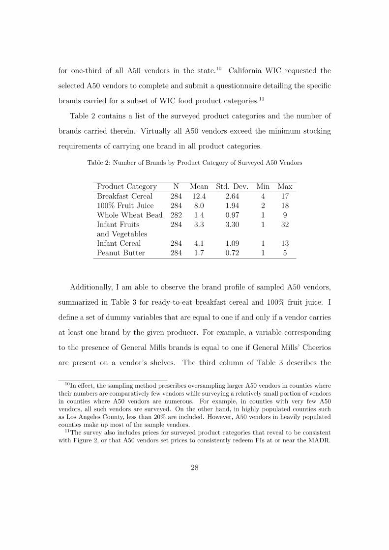
Table 2 contains a list of the surveyed product categories and the number of

brands carried therein. Virtually all A50 vendors exceed the minimum stocking

requirements of carrying one brand in all product categories.

Table 2: Number of Brands by Product Category of Surveyed A50 Vendors

Product Category N Mean Std. Dev. Min MaxBreakfast Cereal 284 12.4 2.64 4 17100% Fruit Juice 284 8.0 1.94 2 18Whole Wheat Bead 282 1.4 0.97 1 9Infant Fruits 284 3.3 3.30 1 32and VegetablesInfant Cereal 284 4.1 1.09 1 13Peanut Butter 284 1.7 0.72 1 5

Additionally, I am able to observe the brand profile of sampled A50 vendors,

summarized in Table 3 for ready-to-eat breakfast cereal and 100% fruit juice. I

define a set of dummy variables that are equal to one if and only if a vendor carries

at least one brand by the given producer. For example, a variable corresponding

to the presence of General Mills brands is equal to one if General Mills’ Cheerios

are present on a vendor’s shelves. The third column of Table 3 describes the

10In effect, the sampling method prescribes oversampling larger A50 vendors in counties wheretheir numbers are comparatively few vendors while surveying a relatively small portion of vendorsin counties where A50 vendors are numerous. For example, in counties with very few A50vendors, all such vendors are surveyed. On the other hand, in highly populated counties suchas Los Angeles County, less than 20% are included. However, A50 vendors in heavily populatedcounties make up most of the sample vendors.

11The survey also includes prices for surveyed product categories that reveal to be consistentwith Figure 2, or that A50 vendors set prices to consistently redeem FIs at or near the MADR.

28

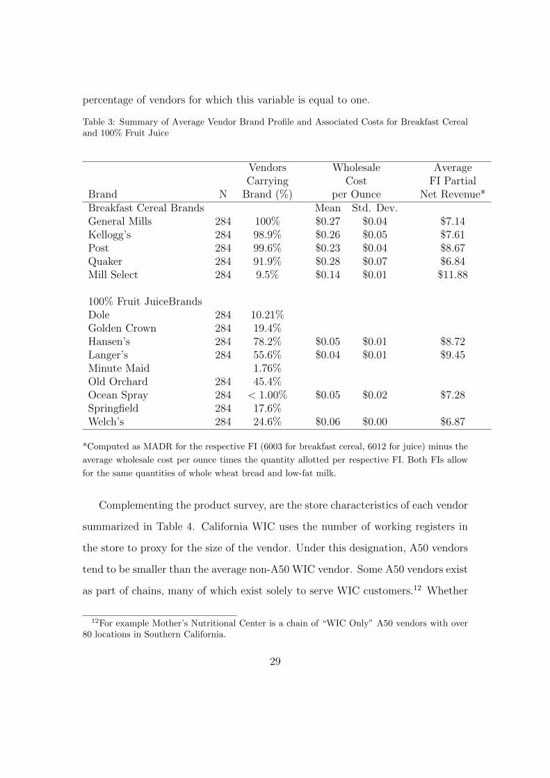
percentage of vendors for which this variable is equal to one.

Table 3: Summary of Average Vendor Brand Profile and Associated Costs for Breakfast Cerealand 100% Fruit Juice

Vendors Wholesale AverageCarrying Cost FI Partial

Brand N Brand (%) per Ounce Net Revenue*Breakfast Cereal Brands Mean Std. Dev.General Mills 284 100% $0.27 $0.04 $7.14Kellogg’s 284 98.9% $0.26 $0.05 $7.61Post 284 99.6% $0.23 $0.04 $8.67Quaker 284 91.9% $0.28 $0.07 $6.84Mill Select 284 9.5% $0.14 $0.01 $11.88

100% Fruit JuiceBrandsDole 284 10.21%Golden Crown 284 19.4%Hansen’s 284 78.2% $0.05 $0.01 $8.72Langer’s 284 55.6% $0.04 $0.01 $9.45Minute Maid 1.76%Old Orchard 284 45.4%Ocean Spray 284 < 1.00% $0.05 $0.02 $7.28Springfield 284 17.6%Welch’s 284 24.6% $0.06 $0.00 $6.87

*Computed as MADR for the respective FI (6003 for breakfast cereal, 6012 for juice) minus the

average wholesale cost per ounce times the quantity allotted per respective FI. Both FIs allow

for the same quantities of whole wheat bread and low-fat milk.

Complementing the product survey, are the store characteristics of each vendor

summarized in Table 4. California WIC uses the number of working registers in

the store to proxy for the size of the vendor. Under this designation, A50 vendors

tend to be smaller than the average non-A50 WIC vendor. Some A50 vendors exist

as part of chains, many of which exist solely to serve WIC customers.12 Whether

12For example Mother’s Nutritional Center is a chain of “WIC Only” A50 vendors with over80 locations in Southern California.

29

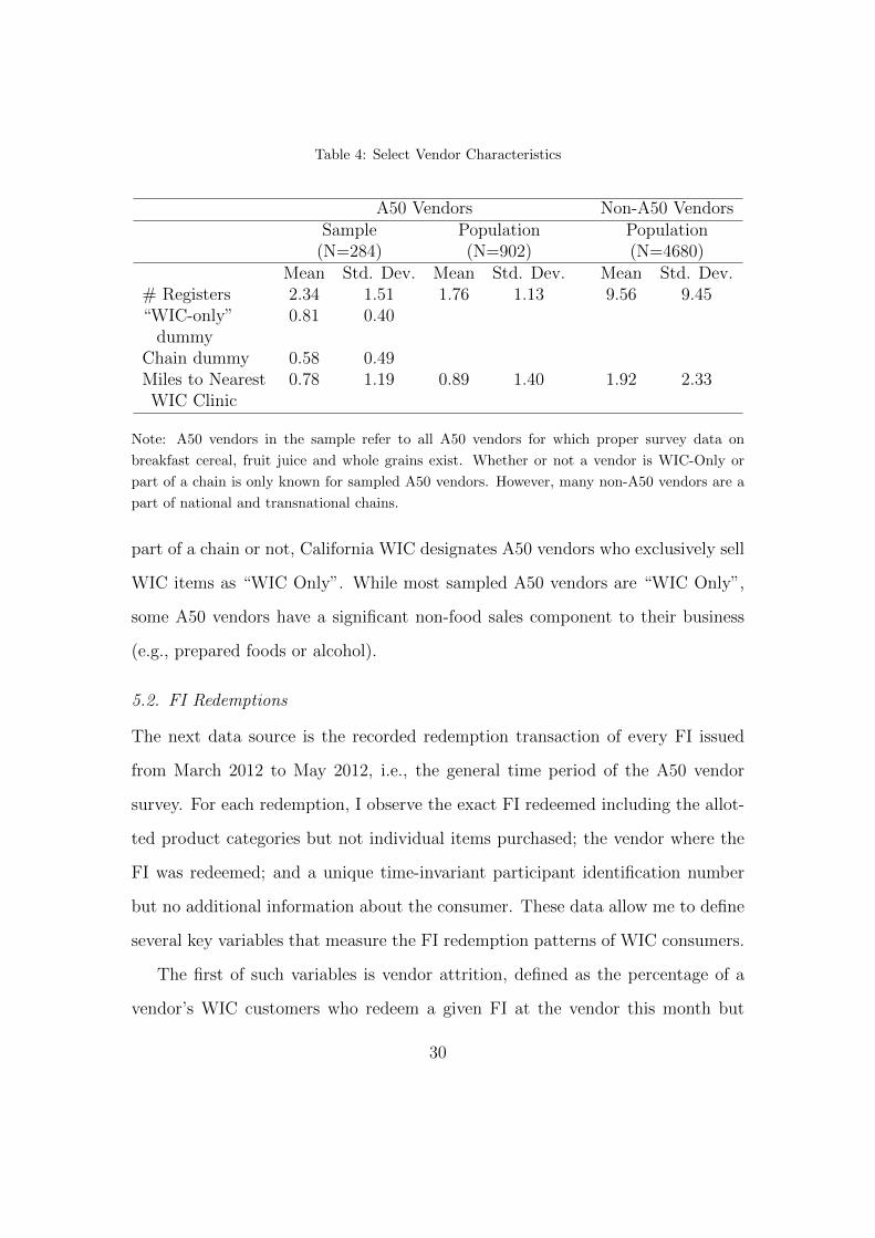
Table 4: Select Vendor Characteristics

A50 Vendors Non-A50 VendorsSample Population Population

(N=284) (N=902) (N=4680)Mean Std. Dev. Mean Std. Dev. Mean Std. Dev.

# Registers 2.34 1.51 1.76 1.13 9.56 9.45“WIC-only” 0.81 0.40

dummyChain dummy 0.58 0.49Miles to Nearest 0.78 1.19 0.89 1.40 1.92 2.33WIC Clinic

Note: A50 vendors in the sample refer to all A50 vendors for which proper survey data on

breakfast cereal, fruit juice and whole grains exist. Whether or not a vendor is WIC-Only or

part of a chain is only known for sampled A50 vendors. However, many non-A50 vendors are a

part of national and transnational chains.

part of a chain or not, California WIC designates A50 vendors who exclusively sell

WIC items as “WIC Only”. While most sampled A50 vendors are “WIC Only”,

some A50 vendors have a significant non-food sales component to their business

(e.g., prepared foods or alcohol).

5.2. FI Redemptions

The next data source is the recorded redemption transaction of every FI issued

from March 2012 to May 2012, i.e., the general time period of the A50 vendor

survey. For each redemption, I observe the exact FI redeemed including the allot-

ted product categories but not individual items purchased; the vendor where the

FI was redeemed; and a unique time-invariant participant identification number

but no additional information about the consumer. These data allow me to define

several key variables that measure the FI redemption patterns of WIC consumers.

The first of such variables is vendor attrition, defined as the percentage of a

vendor’s WIC customers who redeem a given FI at the vendor this month but

30

redeem the same FI elsewhere the following month.13 Vendor attrition is an im-

portant measure of market success in this context, as the overwhelming majority

of customers who commit attrition once do not return to the same vendor again.

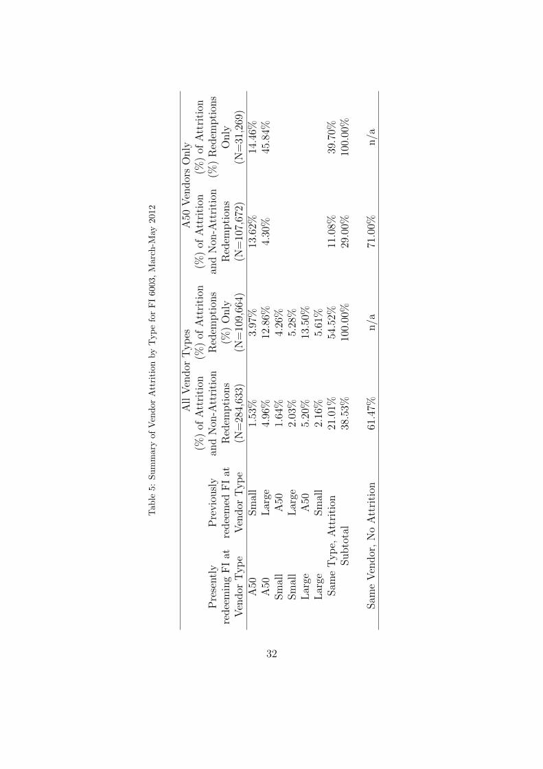
Table 5 summarizes the overall level of vendor attrition, as well as substitution

patterns across vendor types for FI 6003. Because participants typically redeem

all of their monthly allotment of FIs at one vendor at one time, defining attrition

in terms of this one widely redeemed FI captures a representative picture of overall

vendor attrition.

Unconditional on vendor type, WIC consumers commit attrition roughly 38.5%

percent of the time. WIC participants patronizing an A50 vendor, however, are

relatively more loyal, committing attrition for less than 30% of all redemptions

at these vendors. For the most part, participants tend to patronize vendors of

the same type when they choose to patronize another WIC vendor. However,

there is considerable substitution between A50 and large non-A50 vendors, where

participants committing attrition at an A50 vendor are about equally as likely to

patronize either vendor type. On the other hand, the same participants are about

one-third as likely to visit a small non-A50 vendor.

For sampled A50 vendors, I observe that, on average, roughly one-third of all

redemptions of FI 6003 result in attrition, only slightly higher compared to the

population of redemptions (Table 6). Several vendor outliers exist on both ends

of the range. For example, several vendors experience low or no attrition over

the study period. These vendors tend to be relatively isolated vendors that are a

part of WIC-Only chains, however, one such vendor exists primarily as a liquor

13The event of a consumer failing to redeem an FI in the following month is not countedtowards vendor attrition, as the consumer is not in the market in the given month.

31

Tab

le5:

Su

mm

ary

of

Ven

dor

Att

riti

on

by

Typ

efo

rF

I6003,

Marc

h-M

ay2012

All

Ven

dor

Typ

esA

50V

endor

sO

nly

(%)

ofA

ttri

tion

(%)

ofA

ttri

tion

(%)

ofA

ttri

tion

(%)

ofA

ttri

tion

Pre

sentl

yP

revio

usl

yan

dN

on-A

ttri

tion

Red

empti

ons

and

Non

-Att

riti

on(%

)R

edem

pti

ons

redee

min

gF

Iat

redee

med

FI

atR

edem

pti

ons

(%)

Only

Red

empti

ons

Only

Ven

dor

Typ

eV

endor

Typ

e(N

=28

4,63

3)(N

=10

9,66

4)(N

=10

7,67

2)(N

=31

,269

)A

50Sm

all

1.53

%3.

97%

13.6

2%14

.46%

A50

Lar

ge4.

96%

12.8

6%4.

30%

45.8

4%Sm

all

A50

1.64

%4.

26%

Sm

all

Lar

ge2.

03%

5.28

%L

arge

A50

5.20

%13

.50%

Lar

geSm

all

2.16

%5.

61%

Sam

eT

yp

e,A

ttri

tion

21.0

1%54

.52%

11.0

8%39

.70%

Subto

tal

38.5

3%10

0.00

%29

.00%

100.

00%

Sam

eV

endor

,N

oA

ttri

tion

61.4

7%n/a

71.0

0%n/a

32

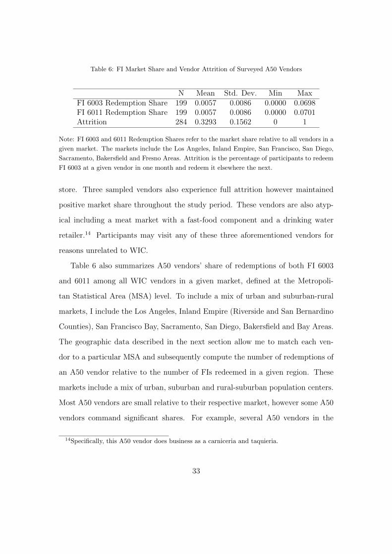
Table 6: FI Market Share and Vendor Attrition of Surveyed A50 Vendors

N Mean Std. Dev. Min MaxFI 6003 Redemption Share 199 0.0057 0.0086 0.0000 0.0698FI 6011 Redemption Share 199 0.0057 0.0086 0.0000 0.0701Attrition 284 0.3293 0.1562 0 1

Note: FI 6003 and 6011 Redemption Shares refer to the market share relative to all vendors in a

given market. The markets include the Los Angeles, Inland Empire, San Francisco, San Diego,

Sacramento, Bakersfield and Fresno Areas. Attrition is the percentage of participants to redeem

FI 6003 at a given vendor in one month and redeem it elsewhere the next.

store. Three sampled vendors also experience full attrition however maintained

positive market share throughout the study period. These vendors are also atyp-

ical including a meat market with a fast-food component and a drinking water

retailer.14 Participants may visit any of these three aforementioned vendors for

reasons unrelated to WIC.

Table 6 also summarizes A50 vendors’ share of redemptions of both FI 6003

and 6011 among all WIC vendors in a given market, defined at the Metropoli-

tan Statistical Area (MSA) level. To include a mix of urban and suburban-rural

markets, I include the Los Angeles, Inland Empire (Riverside and San Bernardino

Counties), San Francisco Bay, Sacramento, San Diego, Bakersfield and Bay Areas.

The geographic data described in the next section allow me to match each ven-

dor to a particular MSA and subsequently compute the number of redemptions of

an A50 vendor relative to the number of FIs redeemed in a given region. These

markets include a mix of urban, suburban and rural-suburban population centers.

Most A50 vendors are small relative to their respective market, however some A50

vendors command significant shares. For example, several A50 vendors in the

14Specifically, this A50 vendor does business as a carniceria and taquieria.

33

Sacramento area have market shares exceeding five-percent of all redemptions in

the region.

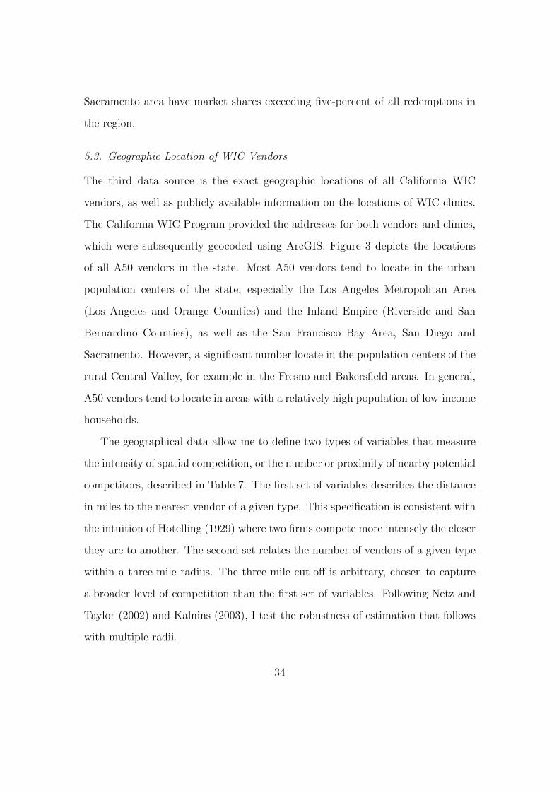
5.3. Geographic Location of WIC Vendors

The third data source is the exact geographic locations of all California WIC

vendors, as well as publicly available information on the locations of WIC clinics.

The California WIC Program provided the addresses for both vendors and clinics,

which were subsequently geocoded using ArcGIS. Figure 3 depicts the locations

of all A50 vendors in the state. Most A50 vendors tend to locate in the urban

population centers of the state, especially the Los Angeles Metropolitan Area

(Los Angeles and Orange Counties) and the Inland Empire (Riverside and San

Bernardino Counties), as well as the San Francisco Bay Area, San Diego and

Sacramento. However, a significant number locate in the population centers of the

rural Central Valley, for example in the Fresno and Bakersfield areas. In general,

A50 vendors tend to locate in areas with a relatively high population of low-income

households.

The geographical data allow me to define two types of variables that measure

the intensity of spatial competition, or the number or proximity of nearby potential

competitors, described in Table 7. The first set of variables describes the distance

in miles to the nearest vendor of a given type. This specification is consistent with

the intuition of Hotelling (1929) where two firms compete more intensely the closer

they are to another. The second set relates the number of vendors of a given type

within a three-mile radius. The three-mile cut-off is arbitrary, chosen to capture

a broader level of competition than the first set of variables. Following Netz and

Taylor (2002) and Kalnins (2003), I test the robustness of estimation that follows

with multiple radii.

34

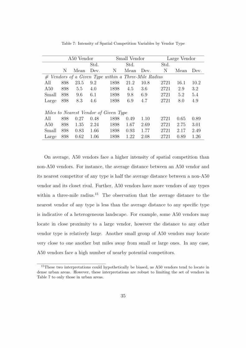
Table 7: Intensity of Spatial Competition Variables by Vendor Type

A50 Vendor Small Vendor Large VendorStd. Std. Std.

N Mean Dev. N Mean Dev. N Mean Dev.# Vendors of a Given Type within a Three-Mile RadiusAll 898 23.5 9.2 1898 21.2 10.8 2721 16.1 10.2A50 898 5.5 4.0 1898 4.5 3.6 2721 2.9 3.2Small 898 9.6 6.1 1898 9.8 6.9 2721 5.2 5.4Large 898 8.3 4.6 1898 6.9 4.7 2721 8.0 4.9

Miles to Nearest Vendor of Given TypeAll 898 0.27 0.48 1898 0.49 1.10 2721 0.65 0.89A50 898 1.35 2.24 1898 1.67 2.69 2721 2.75 3.01Small 898 0.83 1.66 1898 0.93 1.77 2721 2.17 2.49Large 898 0.62 1.06 1898 1.22 2.08 2721 0.89 1.26

On average, A50 vendors face a higher intensity of spatial competition than

non-A50 vendors. For instance, the average distance between an A50 vendor and

its nearest competitor of any type is half the average distance between a non-A50

vendor and its closet rival. Further, A50 vendors have more vendors of any types

within a three-mile radius.15 The observation that the average distance to the

nearest vendor of any type is less than the average distance to any specific type

is indicative of a heterogeneous landscape. For example, some A50 vendors may

locate in close proximity to a large vendor, however the distance to any other

vendor type is relatively large. Another small group of A50 vendors may locate

very close to one another but miles away from small or large ones. In any case,

A50 vendors face a high number of nearby potential competitors.

15These two interpretations could hypothetically be biased, as A50 vendors tend to locate indense urban areas. However, these interpretations are robust to limiting the set of vendors inTable 7 to only those in urban areas.

35

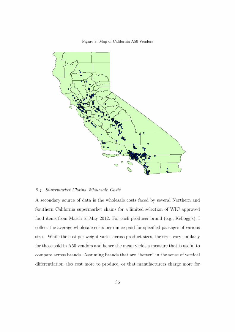
Figure 3: Map of California A50 Vendors

8

each peer group” (7 CFR §246.12(4)). The regulations also require that distinct allowable

redemption and selection criteria be established for A-50 vendors. California has chosen

to satisfy this requirement, in part, by combining all A-50 vendors into a single, statewide

peer group.

Figure 2. Geographic Location of A-50 Vendors

As of January 2012 the state had 4,679 authorized vendors that derived less than

50% of their food revenues from the WIC Program.8 FNS regulations specify that at least

two criteria must be used for establishing peer groups for such vendors, and one criterion

must be geography. Based in part upon recommendations contained in a consultant report

!!!!!!!!!!!!!!!!!!!!!!!!!!!!!!!!!!!!!!!!!!!!!!!!!!!!!!!!8 The Program also authorizes farmers markets across the State as a means to increase participant access to fresh fruits and vegetables. These locations are not included in the authorized vendor total.

5.4. Supermarket Chains Wholesale Costs

A secondary source of data is the wholesale costs faced by several Northern and

Southern California supermarket chains for a limited selection of WIC approved

food items from March to May 2012. For each producer brand (e.g., Kellogg’s), I

collect the average wholesale costs per ounce paid for specified packages of various

sizes. While the cost per weight varies across product sizes, the sizes vary similarly

for those sold in A50 vendors and hence the mean yields a measure that is useful to

compare across brands. Assuming brands that are “better” in the sense of vertical

differentiation also cost more to produce, or that manufacturers charge more for

36

goods highly preferred by many consumers, the wholesale costs offer a proxy of

brand quality (Mussa and Rosen 1978).

Table 3 summarizes the mean wholesale cost for several producer brands of

ready-to-eat breakfast cereal and ready-to-drink 100% fruit juice. Within a prod-

uct category, the average wholesale cost per ounce identifies which brands are

“costly.” For example, the three of the top four leading cereal brands in the United

States (General Mills, Kellogg’s and Quaker) have similarly high costs. On the

other hand, the “off-brand” Mill Select costs roughly half as much. For fruit juice,

Welch’s, a well-known brand, emerges as the costlier brand compared to Hansen’s

and Langer’s.

Combining the wholesale costs with the redemption values and the specific

quantities allowed by FIs, I calculate average partial net revenue measures for FIs

6003 and 6011 (Table 3). Specifically, each entry is the MADR of the FI minus the

average wholesale cost per ounce times the number of ounces allowed by the FI.

Whole-wheat bread and low-fat milk are common to both FIs and hence I ignore

their wholesale costs in this calculation. I observe that when consumers redeem

the most expensive brands, the average partial net revenue is similar across FIs.

For example, a consumer purchasing General Mills cereal and Welch’s juice yield

$7.14 and $6.87, respectively, before the costs of the remaining goods. Carrying

more and better brands in either product category thus yields similar FI profit

margins.

5.5. Preliminary Descriptive Analysis

I focus the analysis on the incentives to optimize the brand profile of ready-to-eat

breakfast cereal and ready-to-drink 100% fruit juice. These product categories are

ideal candidates for study for the following reasons: (a) the strength of incentives

37

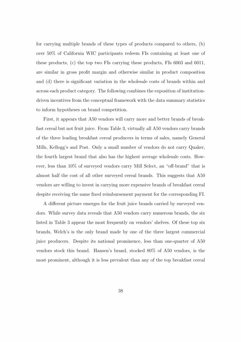
for carrying multiple brands of these types of products compared to others, (b)

over 50% of California WIC participants redeem FIs containing at least one of

these products, (c) the top two FIs carrying these products, FIs 6003 and 6011,

are similar in gross profit margin and otherwise similar in product composition

and (d) there is significant variation in the wholesale costs of brands within and

across each product category. The following combines the exposition of institution-

driven incentives from the conceptual framework with the data summary statistics

to inform hypotheses on brand competition.

First, it appears that A50 vendors will carry more and better brands of break-

fast cereal but not fruit juice. From Table 3, virtually all A50 vendors carry brands

of the three leading breakfast cereal producers in terms of sales, namely General

Mills, Kellogg’s and Post. Only a small number of vendors do not carry Quaker,

the fourth largest brand that also has the highest average wholesale costs. How-

ever, less than 10% of surveyed vendors carry Mill Select, an “off-brand” that is

almost half the cost of all other surveyed cereal brands. This suggests that A50

vendors are willing to invest in carrying more expensive brands of breakfast cereal

despite receiving the same fixed reimbursement payment for the corresponding FI.

A different picture emerges for the fruit juice brands carried by surveyed ven-

dors. While survey data reveals that A50 vendors carry numerous brands, the six

listed in Table 3 appear the most frequently on vendors’ shelves. Of these top six

brands, Welch’s is the only brand made by one of the three largest commercial

juice producers. Despite its national prominence, less than one-quarter of A50

vendors stock this brand. Hansen’s brand, stocked 80% of A50 vendors, is the

most prominent, although it is less prevalent than any of the top breakfast cereal

38

brands.16 Nevertheless it appears that A50 vendors tend to forgo the high cost

fruit juice brands in favor of the lower cost one.

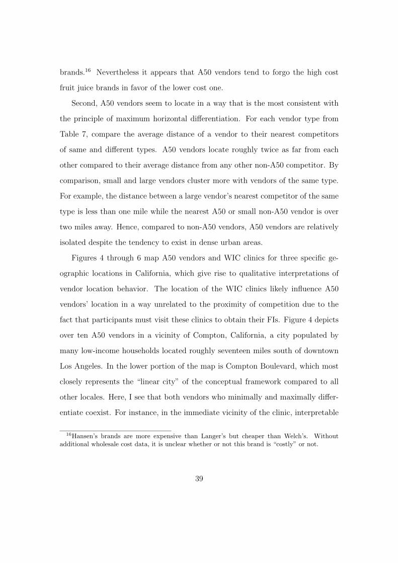
Second, A50 vendors seem to locate in a way that is the most consistent with

the principle of maximum horizontal differentiation. For each vendor type from

Table 7, compare the average distance of a vendor to their nearest competitors

of same and different types. A50 vendors locate roughly twice as far from each

other compared to their average distance from any other non-A50 competitor. By

comparison, small and large vendors cluster more with vendors of the same type.

For example, the distance between a large vendor’s nearest competitor of the same

type is less than one mile while the nearest A50 or small non-A50 vendor is over

two miles away. Hence, compared to non-A50 vendors, A50 vendors are relatively

isolated despite the tendency to exist in dense urban areas.

Figures 4 through 6 map A50 vendors and WIC clinics for three specific ge-

ographic locations in California, which give rise to qualitative interpretations of

vendor location behavior. The location of the WIC clinics likely influence A50

vendors’ location in a way unrelated to the proximity of competition due to the

fact that participants must visit these clinics to obtain their FIs. Figure 4 depicts

over ten A50 vendors in a vicinity of Compton, California, a city populated by

many low-income households located roughly seventeen miles south of downtown

Los Angeles. In the lower portion of the map is Compton Boulevard, which most

closely represents the “linear city” of the conceptual framework compared to all

other locales. Here, I see that both vendors who minimally and maximally differ-

entiate coexist. For instance, in the immediate vicinity of the clinic, interpretable

16Hansen’s brands are more expensive than Langer’s but cheaper than Welch’s. Withoutadditional wholesale cost data, it is unclear whether or not this brand is “costly” or not.

39

as the “market center”, two A50 vendors locate in neighboring shopping centers on

the same side of the street. However, as we move away from the clinic it appears

that the distance between vendors increases geometrically, consistent with maxi-

mal differentiation. While both equilibria are realized empirically, I ask whether

or not one particular equilibrium location strategy is prominent throughout the

state.

Looking at broader geographic regions, the principle of maximum horizontal

differentiation seemingly dominates. One example is Boyle Heights, a low-income

neighborhood of Los Angeles located ten miles east of downtown that is populated

predominantly by Latino households, a key WIC demographic. Figure 5 shows

that while a handful of A50 vendors locate very close to one another, most vendors

exist more dispersed compared to those in Compton. The locale of other urban

areas such as the San Francisco Bay and San Diego Areas, as well as the major

population centers of the otherwise rural Central Valley, Fresno and Bakersfield,

look similar to Figures 4 and 5, suggesting most vendors attempt to distance

themselves from one another.

40

Figure 4: Map of A50 Vendors and WIC Clinics in Compton, CA, Los Angeles MSA

Y

Y

!

!

!!

!

!

!

!

!

!

!

Sources: Esri, HERE, DeLorme, USGS, Intermap, increment PCorp., NRCAN, Esri Japan, METI, Esri China (Hong Kong), Esri(Thailand), TomTom, MapmyIndia, © OpenStreetMapcontributors, and the GIS User Community

Legend! A50 VendorsY WIC Clinics

41

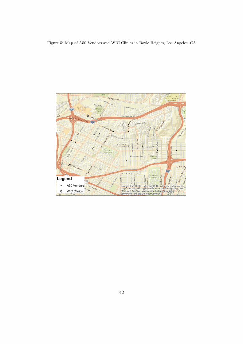
Figure 5: Map of A50 Vendors and WIC Clinics in Boyle Heights, Los Angeles, CA

Y

Y

Y

!

!

!

!

!

!

!

!

!

!

!

!

!

!

!

!

!

!

!

!

!

!

!

!


Legend! A50 Vendors

Y WIC Clinics

42

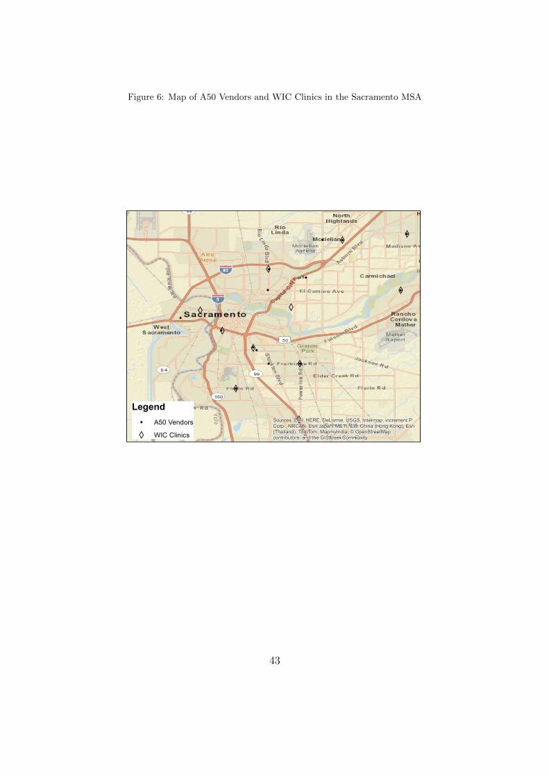
Figure 6: Map of A50 Vendors and WIC Clinics in the Sacramento MSA

YY

Y

Y

Y

Y

Y

Y

Y

Y

Y

!

!

!

!

!

! !

!

!

!

!

!

!

!

!


Legend! A50 VendorsY WIC Clinics

43

Maximal horizontal differentiation is the most striking, however, in the Sacra-

mento region. Figure 6 shows that the vast majority of A50 vendors locate as close

as possible to WIC clinics. Further, few A50 vendors locate nearby to one another.

In fact, the nearest A50 competitor to some vendors in Sacramento is over four

miles away. Incidentally, these vendors also have the highest FI redemptions shares

in their respective market among any other A50 vendors in the state.

The observed substitution patterns among vendor types summarized in Table

5 help form hypotheses on which vendors constitute the set of competitors that

A50 vendors face. WIC participants patronizing an A50 vendor, however, are

relatively more loyal committing attrition for less than 30% of all redemptions

at these vendors. For the most part, participants tend to patronize vendors of

the same type when they choose to patronize another WIC vendor. However,

there is considerable substitution between A50 and large non-A50 vendors, where

participants committing attrition at an A50 vendor are about equally as likely to

patronize either vendor type. On the other hand, the same participants are about

one-third as likely to visit a small non-A50 vendor.

6. Empirical Models

I empirically characterize non-price brand competition in a two-part modeling

approach. The first part establishes the incentives to invest in carrying more and

better brands for some product categories but not others. This part consists of

modeling the conditional mean of vendor attrition and vendor FI market share as

a function of brands and the intensity of spatial competition. The second part

tests whether or not brand competition increases with the intensity of spatial

competition while addressing the endogeneity of vendor location.

The following is relevant for each ensuing model. For vendor i, let brandsi be a

44

vector of the brand variables i.e., the logarithm of the number of brands of a given

product category or dummies for the presence of specific ones; ISCi be either set

of intensity of competition variable described in Table 7; and Xi be a vector of

controls.

6.1. Incentives for Brand Competition

6.1.1. Vendor Attrition

The empirical model of vendor attrition serves as a first-pass test for the existence

of a strong consumer demand response to certain brand variables. Because com-

mitting attrition amounts to exercising a costly option to patronize other vendors,

it is of considerable interest to test whether or not it is driven by vendors’ brand

profile.17 Further, when customers commit vendor attrition, they fail to return to

the vendor the overwhelming majority of the time. If participants are willing to

forgo patronizing a vendor due to an inadequate product offering then there is a

strong incentive to improve variety.

In particular, I estimate the parameters of the following Equation

attritioni = α0 + α1brandsi + α2ISCi + α3Xi + ε1i (11)

For the brand variables most valued by consumers, I expect that α1j < 0 where

α1k ∈ α1 = {α11, α12, . . . , α1j, . . . , α1J} and J is the number of brands. A50 ven-

dors would do well to ensure that their brand profile sufficiently reflects consumer

preferences. Finding α1k = 0 for some variables, however, does not rule out the

possibility that consumers value these attributes. Instead, the marginal utility of

17Relevant costs likely include (but are not necessarily limited to) transportation costs ofvisiting a potentially distant vendor, search costs of finding other vendors and risk associatedwith the possibility that desired brands are not present at the incoming vendor.

45

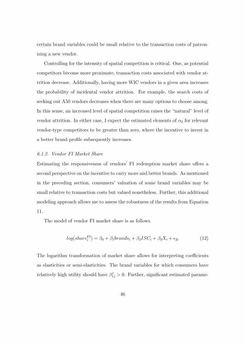
certain brand variables could be small relative to the transaction costs of patron-

izing a new vendor.

Controlling for the intensity of spatial competition is critical. One, as potential

competitors become more proximate, transaction costs associated with vendor at-

trition decrease. Additionally, having more WIC vendors in a given area increases

the probability of incidental vendor attrition. For example, the search costs of

seeking out A50 vendors decreases when there are many options to choose among.

In this sense, an increased level of spatial competition raises the “natural” level of

vendor attrition. In either case, I expect the estimated elements of α2 for relevant

vendor-type competitors to be greater than zero, where the incentive to invest in

a better brand profile subsequently increases.

6.1.2. Vendor FI Market Share

Estimating the responsiveness of vendors’ FI redemption market share offers a

second perspective on the incentive to carry more and better brands. As mentioned

in the preceding section, consumers’ valuation of some brand variables may be

small relative to transaction costs but valued nonetheless. Further, this additional

modeling approach allows me to assess the robustness of the results from Equation

11.

The model of vendor FI market share is as follows.

log(shareFIi ) = β0 + β1brandsi + β2ISCi + β3Xi + ε2i (12)

The logarithm transformation of market share allows for interpreting coefficients

as elasticities or semi-elasticities. The brand variables for which consumers have

relatively high utility should have β11j > 0. Further, significant estimated parame-

46

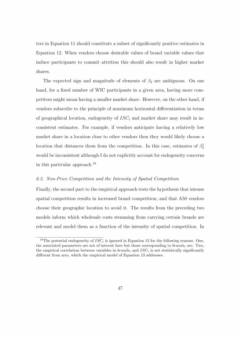
ters in Equation 11 should constitute a subset of significantly positive estimates in

Equation 12. When vendors choose desirable values of brand variable values that

induce participants to commit attrition this should also result in higher market

shares.

The expected sign and magnitude of elements of β2 are ambiguous. On one

hand, for a fixed number of WIC participants in a given area, having more com-

petitors might mean having a smaller market share. However, on the other hand, if

vendors subscribe to the principle of maximum horizontal differentiation in terms

of geographical location, endogeneity of ISCi and market share may result in in-

consistent estimates. For example, if vendors anticipate having a relatively low

market share in a location close to other vendors then they would likely choose a

location that distances them from the competition. In this case, estimates of β12

would be inconsistent although I do not explicitly account for endogeneity concerns

in this particular approach.18

6.2. Non-Price Competition and the Intensity of Spatial Competition

Finally, the second part to the empirical approach tests the hypothesis that intense

spatial competition results in increased brand competition; and that A50 vendors

choose their geographic location to avoid it. The results from the preceding two

models inform which wholesale costs stemming from carrying certain brands are

relevant and model them as a function of the intensity of spatial competition. In

18The potential endogeneity of ISCi is ignored in Equation 12 for the following reasons. One,the associated parameters are not of interest here but those corresponding to brandsi are. Two,the empirical correlation between variables in brandsi and ISCi is not statistically significantlydifferent from zero, which the empirical model of Equation 13 addresses.

47

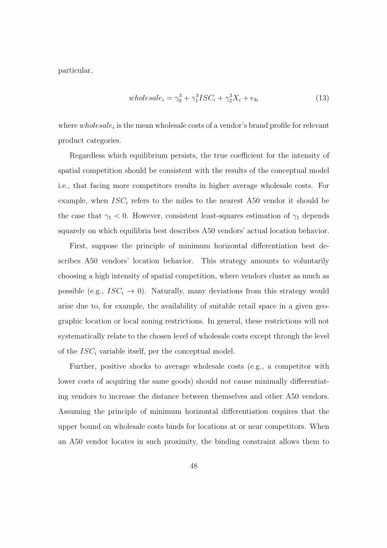
particular,

wholesalei = γ30 + γ3

1ISCi + γ32Xi + ε3i (13)

where wholesalei is the mean wholesale costs of a vendor’s brand profile for relevant

product categories.

Regardless which equilibrium persists, the true coefficient for the intensity of

spatial competition should be consistent with the results of the conceptual model

i.e., that facing more competitors results in higher average wholesale costs. For

example, when ISCi refers to the miles to the nearest A50 vendor it should be

the case that γ1 < 0. However, consistent least-squares estimation of γ1 depends

squarely on which equilibria best describes A50 vendors’ actual location behavior.

First, suppose the principle of minimum horizontal differentiation best de-

scribes A50 vendors’ location behavior. This strategy amounts to voluntarily

choosing a high intensity of spatial competition, where vendors cluster as much as

possible (e.g., ISCi → 0). Naturally, many deviations from this strategy would

arise due to, for example, the availability of suitable retail space in a given geo-

graphic location or local zoning restrictions. In general, these restrictions will not

systematically relate to the chosen level of wholesale costs except through the level

of the ISCi variable itself, per the conceptual model.

Further, positive shocks to average wholesale costs (e.g., a competitor with

lower costs of acquiring the same goods) should not cause minimally differentiat-

ing vendors to increase the distance between themselves and other A50 vendors.

Assuming the principle of minimum horizontal differentiation requires that the

upper bound on wholesale costs binds for locations at or near competitors. When

an A50 vendor locates in such proximity, the binding constraint allows them to

48

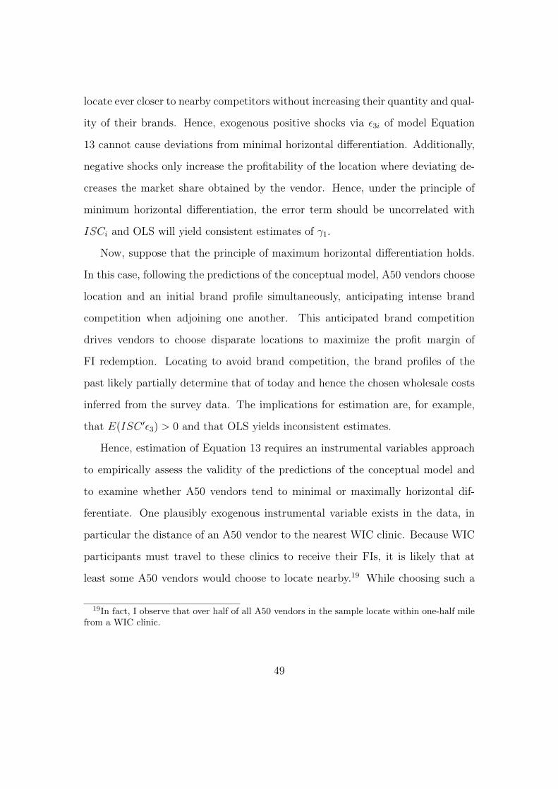
locate ever closer to nearby competitors without increasing their quantity and qual-

ity of their brands. Hence, exogenous positive shocks via ε3i of model Equation

13 cannot cause deviations from minimal horizontal differentiation. Additionally,

negative shocks only increase the profitability of the location where deviating de-

creases the market share obtained by the vendor. Hence, under the principle of

minimum horizontal differentiation, the error term should be uncorrelated with

ISCi and OLS will yield consistent estimates of γ1.

Now, suppose that the principle of maximum horizontal differentiation holds.

In this case, following the predictions of the conceptual model, A50 vendors choose

location and an initial brand profile simultaneously, anticipating intense brand

competition when adjoining one another. This anticipated brand competition

drives vendors to choose disparate locations to maximize the profit margin of

FI redemption. Locating to avoid brand competition, the brand profiles of the

past likely partially determine that of today and hence the chosen wholesale costs

inferred from the survey data. The implications for estimation are, for example,

that E(ISC ′ε3) > 0 and that OLS yields inconsistent estimates.

Hence, estimation of Equation 13 requires an instrumental variables approach

to empirically assess the validity of the predictions of the conceptual model and

to examine whether A50 vendors tend to minimal or maximally horizontal dif-

ferentiate. One plausibly exogenous instrumental variable exists in the data, in

particular the distance of an A50 vendor to the nearest WIC clinic. Because WIC

participants must travel to these clinics to receive their FIs, it is likely that at

least some A50 vendors would choose to locate nearby.19 While choosing such a

19In fact, I observe that over half of all A50 vendors in the sample locate within one-half milefrom a WIC clinic.

49

location may reduce the transportation costs associated with FI redemption for

some participants, WIC clinics do not necessarily neighbor all participants’ homes.

In this case, some A50 vendors may do well to locate away from the clinic and

closer to areas densely populated in WIC participants. Consequently, proximity

to a WIC clinic does not inherently relieve A50 vendors of the pressure to engage

in brand competition. Instead, the distance to the nearest clinic affects the chosen

wholesale costs only insofar as it affects the location decision of the vendor.

6.3. Spatial Error Structure

It is likely that shocks in Equations 11-13 are common to neighboring vendors

to some extent. For example, heavy traffic along a certain freeway or regional

variation in wholesales costs could impact all vendors within a vicinity. The con-

sequences of failing to properly model spatial dependence include inefficient pa-

rameter estimates, biased t-statistics, and hence incorrect inference (Anselin 2006).

To account for the possibility of spatial dependence, I use spatial econometrics to

model the error terms of Equations 11-13.

In particular, I assume the εki, k = 1, 2, 3, take the functional form of a spatial

error model (SEM). That is,

εki = ρWεki + vki (14)

where vki is identically and independently distributed and W is an inverse-distance

row-normalized weighting matrix. This functional form allows for spatial depen-

dence of εki among vendors that dissipates as the distance between two vendors

increases.

Empirical model estimation in conjunction with a SEM follows Kelejian and

50

Prucha (1998). This approach is a generalized spatial two-stage least squares

(GS2SLS) procedure, which follows similarly to Cochrane-Orcutt procedures used

in time series econometrics.20 First, Equation 13, for example, is estimated by

two-stage least squares using spatially lagged exogenous variables as instruments.

The purpose of this auxiliary regression is to estimate ρ of Equation 14 and,

subsequently, Equation 13 is re-estimated using ρ̂ via the generalized method of

moments (GMM). Next, a Cochrane-Orcutt transformed version of Equation 13

using the previous estimate of ρ is re-estimated via two-stage least squares Lastly,

ρ is re-estimated using efficient GMM.

In the event that independent variables fail to be orthogonal to the error terms

of Equations 11-13, GS2SLS is easily modified to accommodate additional endoge-

nous variables (Drukker, Prucha and Raciborski 2013). In this case, excluded

exogenous variables and their spatial lags serve as instrumental variables in ad-

dition to the spatially lagged included exogenous variables, as described above.

Otherwise, the GS2SLS estimation proceeds normally as outlined in Kelejian and

Prucha (1998).

7. Results

The following presents estimation results of the three empirical models. Each

subsection interprets findings and discusses the veracity of the results in light of

specific issues that arise in estimation. The first two models establish an incentive

to compete in brands, while suggesting which types of brands and competitors

are salient. These findings motivate the specification and interpretation of the

20It is worth noting that Das, Kelejian and Prucha (2003) find the GS2SLS to be consistentand nearly as efficient as popular maximum likelihood in small sample Monte Carlo experiments.Hence, GS2LS can be relied upon to provide reliable estimates of parameters of interest.

51

third empirical model of wholesale costs as a function of the intensity of spatial

competition.

7.1. Incentives for Brand Competition

The following details the results of the estimated vendor attrition and vendor FI

market share models. Additionally, I defend the assumption of exogeneity of key

regressors and the implications for results.

7.1.1. Vendor Attrition

Table 8 presents the estimates of the vendor attrition model in Equation 11.21 The

preferred specifications of the vendor attrition model are contained in columns (e)

and (f). For specifications (a) and (b), a subset of the control variable are indi-

vidually and jointly insignificant while correlated with the brand variables. That

these variables correlate is unsurprising as, for example, intuitively a “WIC-Only”

store should carry more WIC food brands, all else equal. Omitting the offending

variables from the model to reduce multicollinearity affects the significance of the

coefficient estimates for the brand variables while preserving their magnitudes.

Models (c) and (d) remove only the brand variables, revealing the joint insignifi-

cance of the select control variables to be robust. Hence, I focus my discussion on

the results of specifications (e) and (f) of the vendor attrition model.

The reduction in attrition related to even small increases in the number of cereal

brands is dramatically large. Vendors with the lowest number of brands, where

unit increases are large in percentage terms, also experience the highest levels of

21I test for the presence of spatial autocorrelation using Moran’s I Statistic formulated as I =(ε̂′kWε̂k/S0)/(ε̂′k ε̂k/n) where S0 =

∑i

∑j wij (Anselin 2006). I fail to reject the null hypothesis

of no spatial autocorrelation in the error term (i.e., ρ = 0) and hence I do not present SEMresults.

52

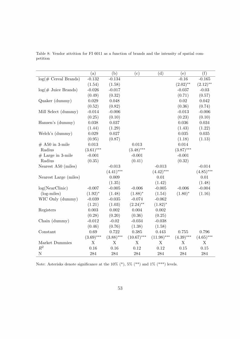
Table 8: Vendor attrition for FI 6011 as a function of brands and the intensity of spatial com-petition

(a) (b) (c) (d) (e) (f)

log(# Cereal Brands) -0.132 -0.134 -0.16 -0.165(1.54) (1.58) (2.02)∗∗ (2.12)∗∗

log(# Juice Brands) -0.026 -0.017 -0.037 -0.03(0.49) (0.32) (0.71) (0.57)

Quaker (dummy) 0.029 0.048 0.02 0.042(0.52) (0.82) (0.36) (0.74)

Mill Select (dummy) -0.014 -0.006 -0.013 -0.006(0.25) (0.10) (0.23) (0.10)

Hansen’s (dummy) 0.038 0.037 0.036 0.034(1.44) (1.29) (1.43) (1.22)

Welch’s (dummy) 0.029 0.027 0.035 0.035(0.95) (0.87) (1.18) (1.13)

# A50 in 3-mile 0.013 0.013 0.014Radius (3.61)∗∗∗ (3.48)∗∗∗ (3.87)∗∗∗

# Large in 3-mile -0.001 -0.001 -0.001Radius (0.35) (0.41) (0.32)

Nearest A50 (miles) -0.013 -0.013 -0.014(4.41)∗∗∗ (4.42)∗∗∗ (4.85)∗∗∗

Nearest Large (miles) 0.009 0.01 0.01(1.35) (1.42) (1.48)

log(NearClinic) -0.007 -0.005 -0.006 -0.005 -0.006 -0.004(log-miles) (1.92)∗ (1.48) (1.88)∗ (1.54) (1.80)∗ (1.16)

WIC Only (dummy) -0.039 -0.035 -0.074 -0.062(1.21) (1.03) (2.24)∗∗ (1.82)∗

Registers 0.003 0.002 0.004 0.002(0.28) (0.20) (0.36) (0.25)

Chain (dummy) -0.012 -0.02 -0.034 -0.038(0.46) (0.76) (1.38) (1.58)

Constant 0.69 0.722 0.385 0.443 0.755 0.796(3.69)∗∗∗ (3.88)∗∗∗ (10.67)∗∗∗ (11.98)∗∗∗ (4.39)∗∗∗ (4.65)∗∗∗

Market Dummies X X X X X XR2 0.16 0.16 0.12 0.12 0.15 0.15N 284 284 284 284 284 284

Note: Asterisks denote significance at the 10% (*), 5% (**) and 1% (***) levels.

53

attrition. Thus the logarithmic transformation may overstate the average effect

of increasing cereal brands. Nevertheless, this coefficient’s sign and statistical

significance is robust to estimates forgoing the transformation. No other brand

variable is statistically significant in any specification. Participants may still value

these brand characteristics, although the strength of the preference is at most weak

compared to that for variety of cereal brands.

The incentive to invest in brands predictably grows as potential competitors

become more numerous and less distant. Results suggest a high degree of competi-

tion between A50 vendors relates to higher rates of vendor attrition. For example,

a vendor with an additional A50 competitor within a three-mile radius sees a

1.4% increase in attrition, on average. Naturally, when two competing vendors

are nearby one another the cost of going to one versus another is relatively small.

The effect of the intensity of spatial competition with other A50 vendors is small,

however, compared to the estimated coefficient for the logarithm of the number of

breakfast cereal brands.

The proximity of large vendors, on the other hand, appears to have no effect,

indicating A50 vendors are not directly competing with large traditional retail-

ers. Additionally, I exclude spatial variables pertaining to small non-A50 vendors

due to the relatively little level of substitution between these and A50 vendors

observed in Table 5. However, the results of Table 8 are unchanged by including

small vendors although point estimates for their effects on vendor attrition are sta-

tistically insignificant. Lastly, despite the fact that participants must physically

obtain FIs from local WIC clinics, a vendor’s distance to them has a limited effect

on attrition. This finding may be due to the fact that vendors tend to locate near

clinics anyway and hence the relevant variable predicting attrition behavior is the

54

intensity of spatial competition.

7.1.2. Vendor FI Market Share

I use two definitions of the dependent variable to test whether the results in Table

9 are specific to the FI for which share is measured.22 FI 6003 allows for 36 ounces

of breakfast cereal while FI 6011 has two 64 ounce bottles of fruit juice, and over

50% of all WIC participants receive at least one of these FIs. Coefficient estimates

are nearly identical across both market share definitions, indicating the observed

incentives for competition apply broadly to a vendor’s market performance and

are not idiosyncratic to specific FIs.

Consistent with estimates in Table 8, the number of breakfast cereal brands

relates positively to higher market shares of all FIs (Table 9). The share of FI re-

demptions is relatively elastic to the number of cereal brands, indicating a strong

incentive to increase variety. Likewise, the number of juice brands has no statis-

tically significant relationship with any measure of market share. Thus, there is

seemingly no strong incentive to compete in variety of brands other than breakfast

cereal.

Somewhat in departure from estimates in Table 8, vendors who carry varieties

of the Quaker brand of cereal, but not Mill Select, tend to have higher shares. With

respect to breakfast cereal brands, vendors see an increase in market share when

they invest in carrying expensive brands (e.g., Quaker) rather than the cheapest

ones (e.g., Mill Select). This finding is reflected in the average brand profile of A50

vendors where the overwhelming majority of such vendors carry high wholesale cost

brands.

22Likewise in the vendor attrition model, I find no evidence of spatial autocorrelation.

55

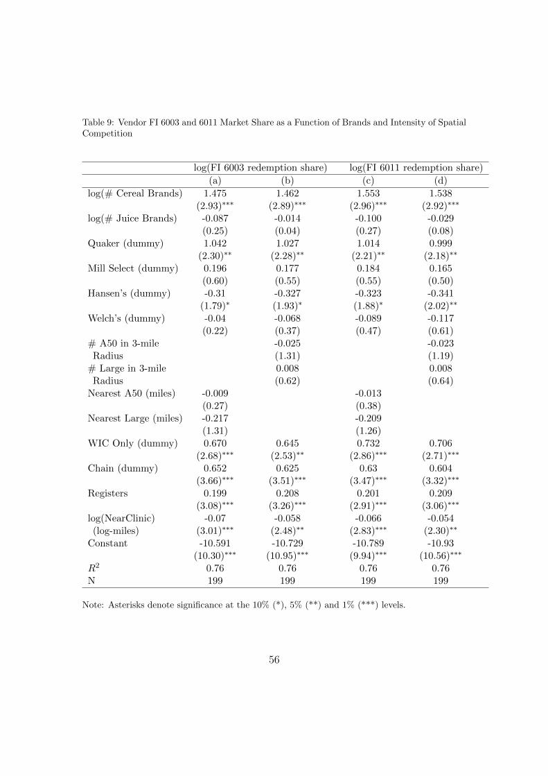
Table 9: Vendor FI 6003 and 6011 Market Share as a Function of Brands and Intensity of SpatialCompetition

log(FI 6003 redemption share) log(FI 6011 redemption share)

(a) (b) (c) (d)

log(# Cereal Brands) 1.475 1.462 1.553 1.538(2.93)∗∗∗ (2.89)∗∗∗ (2.96)∗∗∗ (2.92)∗∗∗

log(# Juice Brands) -0.087 -0.014 -0.100 -0.029(0.25) (0.04) (0.27) (0.08)

Quaker (dummy) 1.042 1.027 1.014 0.999(2.30)∗∗ (2.28)∗∗ (2.21)∗∗ (2.18)∗∗

Mill Select (dummy) 0.196 0.177 0.184 0.165(0.60) (0.55) (0.55) (0.50)

Hansen’s (dummy) -0.31 -0.327 -0.323 -0.341(1.79)∗ (1.93)∗ (1.88)∗ (2.02)∗∗

Welch’s (dummy) -0.04 -0.068 -0.089 -0.117(0.22) (0.37) (0.47) (0.61)

# A50 in 3-mile -0.025 -0.023Radius (1.31) (1.19)

# Large in 3-mile 0.008 0.008Radius (0.62) (0.64)

Nearest A50 (miles) -0.009 -0.013(0.27) (0.38)

Nearest Large (miles) -0.217 -0.209(1.31) (1.26)

WIC Only (dummy) 0.670 0.645 0.732 0.706(2.68)∗∗∗ (2.53)∗∗ (2.86)∗∗∗ (2.71)∗∗∗

Chain (dummy) 0.652 0.625 0.63 0.604(3.66)∗∗∗ (3.51)∗∗∗ (3.47)∗∗∗ (3.32)∗∗∗

Registers 0.199 0.208 0.201 0.209(3.08)∗∗∗ (3.26)∗∗∗ (2.91)∗∗∗ (3.06)∗∗∗

log(NearClinic) -0.07 -0.058 -0.066 -0.054(log-miles) (3.01)∗∗∗ (2.48)∗∗ (2.83)∗∗∗ (2.30)∗∗

Constant -10.591 -10.729 -10.789 -10.93(10.30)∗∗∗ (10.95)∗∗∗ (9.94)∗∗∗ (10.56)∗∗∗

R2 0.76 0.76 0.76 0.76N 199 199 199 199

Note: Asterisks denote significance at the 10% (*), 5% (**) and 1% (***) levels.

56

Fruit juices, on the other hand, see no such positive relationship between car-

rying either the expensive or inexpensive brands with share. In fact, carrying

Hansen’s brand juice–the low cost brand–correlates to a decrease in market share.

This may suggest that carrying only cheap brands of any product category is un-

desirable. Nevertheless, vendors have no strong incentive to invest in stocking the

higher cost juice brand. These findings are consistent with the average fruit juice

brand profile of A50 vendors where no one brand clearly dominates and expensive

brands are carried infrequently. Hence, I find strong evidence of vendor’s incentive

to compete in brands only for the product categories most valued by consumers.

Another striking result is that no measure of the intensity of spatial competition

significantly relates to vendor FI market share. This finding is consistent with the

fact that many A50 vendors tend to locate in regions dense with WIC participants

and experience high market share as a result. Instead of reducing a vendor’s share

of a likely relatively fixed amount of WIC business, intense spatial competition is

a zero-sum game where participants are more likely to shop around as opposed to

shift their patronage permanently. On the other hand, vendors with few competi-

tors may also have comparatively few WIC clients and, thus, the impact of the

intensity of spatial competition on market share is limited. The importance of the

vendor attrition variable, then, is to capture the degree of customer loyalty an A50

vendor experiences.

Estimated coefficients of other control variables take on the expected sign.

For example, it is unsurprising that WIC only stores, who are the most likely to

excel in unobserved store experience characteristics, on average have a higher FI

redemption share. Larger vendors that are part of a chain also redeem more FIs

perhaps due to greater inventory and more effective management. Additionally,

57

vendors closer to local WIC clinics where participants receive FIs also tend to have

a slightly higher market share.

7.1.3. Exogeneity of Key Regressors

The assumption that brand and spatial variables are exogenous in the empirical

framework requires defense. The brand variables especially necessitate such a dis-

cussion, as I argue that vendors will choose non-price characteristics strategically.

This modeling choice follows much of the discrete choice literature where the treat-

ment of the endogeneity of prices is the main concern (Nevo 2000). In essence, I

argue that the brand and intensity of spatial competition variables are not updated

on a continuous basis and are predetermined with respect to the measured market

outcomes. The following discusses the veracity of these findings in light of several

specific issues of endogeneity.

First, vendor-specific omitted variables potentially correlated with WIC brands

could bias estimates of the respective parameters of brands in Equations 11 and

12. Specifically, none of the included regressors will fully capture store experience,

such as cleanliness, ease of shopping experience and good customer service. Nearly

all consumers of all types rank such characteristics as nearly as important as prices

and variety in choosing their primary food retail outlet (Progressive Grocer 2010).

It may be that price inelastic WIC participants shopping at A50 vendors have

a stronger preference for store experience, as they forgo the greater variety of

the large vendor. Additionally, I do not observe certain qualities of other product

categories not considered in this analysis. For example, the expiration dates of milk

or the freshness of fruits and vegetables sold independent of FIs could correlate to

the quantity and quality of other brands.23

23Participants may receive cash value vouchers (CVVs) in addition to FIs to purchase fresh

58

The consequences of such omitted variables bias would still be consistent with

the idea that vendors will engage in non-price competition when they cannot com-

pete in price. Further, the variance in magnitude of hypothetical estimate bias

across product categories manifests in in a way that is consistent with the in-

terpretation that carrying more and better brands is more important for some

product categories than others.24 However, there is still reason yet to believe

that brand variables rather than omitted store experience ones drive the results

of the brands parameters. In particular, improving the quality of store experience

is likely less costly than improving the vendor’s brand profile. Increasing overall

selection of goods requires incurring significant fixed costs (Ellickson 2006) and

managing inventory to ensure brands are consistently available is costly as well

(Matsa 2011). Improving the consumer shopping experience of A50 vendors would

then likely precede any investment in increasing the quantity and quality of brands.

If true, then the correlation between brand variables and omitted store experience

variables–and hence the error term–would be relatively small.

Second, codetermination between the attrition and brand variables may per-

sist. A vendor who competes in brands would likely improve his brand profile in

response to an observed increase in attrition. However, the presence of this type of

endogeneity is likely unproblematic for the following reasons. Vendors responding

positively in brands to an upward shock in attrition would only serve to attenuate

key results.25 Further, if vendors tend to maximally differentiate geographically,

fruits and vegetables. The CVVs differ from FIs in that participants have a fixed cash amountto spend.

24In other words, if the bias affects each brand variable equally I reject the null hypothesis thateach parameter is the same. If the bias varies by brand variable then my original explanationremains valid.

25The interpretation of results would also remain the same by the same argument of theprevious footnote.

59

then it is likely that brands are not updated on a continuous basis. Instead, an

initially modest brand profile would persist as long as the vendors remained iso-

lated.

To provide evidence for the claim that vendors’ brand profiles are relatively

fixed, I am able to obtain additional prior FI redemption data from October 2009

to February 2012 and define vendor attrition over this period. First, the results

in Table 8 are robust to using vendor attrition dating back to June 2011, nine

months prior to the in-store survey. This finding suggests the brand profile re-

sponds slowly to competitive changes. Second, past attrition prior to June 2011

then should serve as a plausibly exogenous instrument for present vendor attrition

rates. However, first-stage regressions indicate that past attrition is in fact a weak

instrument.26 Nevertheless the empirical results indicate that vendors have an

incentive to compete in brands, while their observed brand profile combined with

the upcoming results of the second part of the empirical approach suggests they

do in fact engage in this behavior. However, this incentive does not readily appear

in explaining measured brand variables as a function of past vendor attrition.

7.2. Non-Price Competition and the Intensity of Spatial Competition

Table 10 presents the estimated coefficients of Equation 13. In general, estimation

techniques that do not account for endogeneity in the intensity of spatial competi-

tion appear to yield inconsistent estimates. For example, compare the magnitudes

of the ISC coefficient from models (a) to (c), ignoring the statistical insignificance

of both estimates for the moment. Only the coefficient estimate of the 2SLS model

is consistent with the theoretical prediction that non-price competition intensifies

26F-statistics from first-stage regressions are consistently below 10 for most permutations ofmonthly vendor attrition variables ranging from October 2009 to February 2012.

60

with greater proximity of competitors. Hence, initial evidence suggests that A50

vendors tend to engage in maximum horizontal differentiation.

However, both estimates are clearly statistically insignificant. Consequently,

Hausman-type tests fail to the reject null hypothesis of the consistency of OLS

at commonly accepted significance levels. Estimating Equation 13 within a SEM

framework, I find statistically significant positive estimated values for specifications

(e) through (h).27 This finding indicates spatial autocorrelation in the unobserved

factors influencing chosen wholesales costs. Hence the estimates in (a) through (d)

are inefficient, requiring the GS2SLS-SEM approach for inference.

Additionally, “WIC Only” stores tend to carry less expensive brands, on av-

erage, although this result is not robust to specification. This finding may arise

due to the fact that “WIC Only” vendors are the most likely to carry the “off”

breakfast cereal brands which tends to lower the average wholesale costs. Even

though few consumers would prefer these brands to nationally recognized ones,

the opportunity cost of shelving space for WIC-approved cereals will be lower for

these vendors compared to non-“WIC Only” vendors, all else equal. This expla-

nation may also account for the insignificance of the coefficient for the number of

registers. However, it is intuitive that chain A50 vendors have better brands, on

average, as they are likely able to purchase better brands for a cheaper unit price.

8. Conclusion

Food retailers who do not compete in price have an incentive to invest in carrying

more and better brands to maintain customers and increase their market share.

However, carrying more and better brands is costly, and retailers tend to locate

27I define the weighting matrix W for only those variables for which market is defined toexclude the possibility of results biased by thin markets.

61

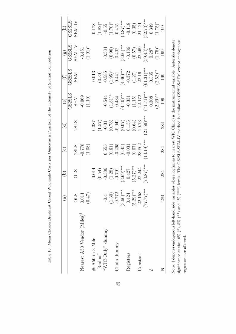
Tab

le10

:M

ean

Ch

osen

Bre

akfa

stC

erea

lW

hole

sale

Cost

sp

erO

un

ceas

aF

un

ctio

nof

the

Inte

nsi

tyof

Sp

ati

al

Com

pet

itio

n

(a)

(b)

(c)

(d)

(e)

(f)

(g)

(h)

GS2S

LS

GS2S

LS

GS2S

LS

GS2S

LS

OL

SO

LS

2SL

S2S

LS

SE

MSE

MSE

M-I

VSE

M-I

V

Nea

rest

A50

Ven

dor

(Miles

)†0.

014

-0.7

78-0

.069

-0.4

51(0

.47)

(1.0

8)(1

.10)

(1.9

1)∗

#A

50in

3-M

ile

-0.0

140.

387

-0.0

130.

178

Rad

ius†

(0.5

4)(1

.57)

(0.3

9)(1.8

2)∗

“WIC

-Only

”dum

my

-0.4

-0.3

860.

555

-0.3

1-0

.544

-0.5

85-0

.334

-0.5

5(1

.30)

(1.2

8)(0

.61)

(0.7

8)(1.8

1)∗

(1.9

5)∗

(0.9

6)(1.7

0)∗

Chai

ndum

my

-0.7

72-0

.791

-0.2

95-0

.042

0.43

40.

441

0.40

20.

415

(3.6

6)∗∗∗

(3.6

9)∗∗∗

(0.4

5)(0

.07)

(4.4

0)∗∗∗

(4.4

6)∗∗∗

(3.6

6)∗∗∗

(3.8

7)∗∗∗

Reg

iste

rs0.

424

0.42

7-0

.031

0.13

5-0

.331

-0.3

72-0

.186

-0.1

18(5.2

9)∗∗∗

(5.2

7)∗∗∗

(0.0

7)(0

.64)

(1.1

5)(1

.27)

(0.5

7)(0

.35)

Con

stan

t22

.158

22.2

4423

.862

20.7

322

.172

22.1

922

.469

21.1

21(7

7.77

)∗∗∗

(73.

87)∗∗∗

(14.

19)∗∗∗

(21.

59)∗∗∗

(71.

71)∗∗∗

(61.

31)∗∗∗

(59.

43)∗∗∗

(32.

73)∗∗∗

ρ̂0.

308

0.33

50.

287

0.34

9(2.2

9)∗∗

(2.5

2)∗∗

(1.7

5)∗

(1.7

5)∗

N28

428

428

428

419

919

919

919

9

Not

e:†

den

otes

end

ogen

ous

left

-han

dsi

de

vari

ab

les

wh

ere

log(m

iles

ton

eare

stW

ICC

lin

ic)

isth

ein

stru

men

talva

riab

le.

Ast

eris

ks

den

ote

sign

ifica

nce

atth

e10

%(*

),5%

(**)

and

1%(*

**)

leve

ls.

Th

eG

S2S

LS

-SE

M-I

Vm

eth

od

issi

mil

ar

toG

S2S

LS

-SE

Mex

cep

ten

dogen

ou

s

regr

esso

rsar

eal

low

ed.

62

themselves in a way that minimizes the necessity to engage in such measures.

Using A50 vendors, an organic example of a non-price competing firm, I find that

they compete in brands for least one product category. Carrying many brands

of breakfast cereal reduces the rate of vendor attrition and increases their market

share in conjunction with having more expensive brands. Having more and better

brands in this category effectively reduces the intensity of spatial competition that

an A50 vendor faces by attempting to increase its differentiation relative to rivals

in a quality dimension. However, I do not find this result for fruit juice brands

despite similar profit margins for respective FIs allowing for these goods. This

finding is consistent with the conclusions of the demand literature (Nevo 2000;

Huang, Perloff and Villas-Boas 2006; Chidmi and Lopez 2007) where consumers

reveal a strong willingness-to-pay for particular breakfast cereal brands but not

juice brands.

My findings are consistent with a theoretical model in the tradition of Hotelling

(1929) that supports either the principle of minimum or maximum horizontal (i.e.,

geographic) differentiation as equilibria when faced with pure non-price competi-

tion. Overall, it appears that the array of approved food items under California

WIC allows for intense non-price competition and, hence, I observe that ven-

dors tend to maximally differentiate. Interestingly, this outcome is observationally

equivalent to the case where the allowed wholesale costs for brand profiles is unlim-

ited. This suggests that, given fixed payments for FIs, the competitive environment

of FI redemption induces vendors to choose locations specifically to reduce their

own costs and hence the costs of the Program.

The ability to choose location while competing using a vertical quality com-

ponent differentiates my work from other applications in non-price competition.

63

Namely, my findings differ from those of studies of the airline industry where firms

compete in quality until exhaustion of profits. The ability to differentiate in hor-

izontal space allows the A50 vendors to earn positive profits, in theory, and thus

mimics location behavior under price competition. Additionally, I show that non-

price dimensions are important as competitive “ends” in and of themselves, as

opposed to a means to increase prices charged to consumers.

The observation that participants highly value the opportunity to purchase

more and better brands should be of interest to policymakers and Program admin-

istrators. Recent federal budget cuts reduced funding to the Program nationwide

and cost-containment is a high priority among program administrators. To the ex-

tent that any policy changes affect the brands that WIC vendors carry, reductions

in the welfare of participants may occur. For example, if California WIC admin-

istrators decide to cut costs by limiting the availability of costly breakfast cereal

brands for purchase then consumer welfare would dramatically decrease. Existing

WIC participants may fail to fully redeem their FIs if no offered brands are pre-

ferred nothing at all. Additionally, prospective participants may be dissuaded from

participation in the Program if they are unable to purchase the specific goods they

value the most. On the other hand, restricting the costs of allowable juice brands

would have minimal consequences for welfare or participation and hence may be

better targets for cost reduction measures, although only a minority of vendors

are seen to carry expensive juice brands. Further, restricting brand choice of rel-

evant product categories available for non-price competition may induce vendors

to relocate to minimally differentiate in space. The realization of such an outcome

may exacerbate issues of food access for WIC consumers, where fewer unique A50

vendor locations are available. Policymakers would do well to appreciate the im-

64

portance of brand and non-price attributes broadly to and food retailers’ market

outcomes, the welfare of WIC participants and Program access.

9. References

[1] Anselin, L. 2006. “Spatial Econometrics.” Palgrave Handbook of Economet-

rics: Volume 1, Econometric Theory. 901-969.

[2] Anselin, Luc. 2010. “Thirty years of spatial econometrics.” Papers in Regional

Science. 89(1): 3-25.

[3] Arcia, G.T., L.A. Crouch, and R.A. Kulka. 1990. “Impact of the WIC Program

on Food Expenditures.” American Journal of Agricultural Economics. 72(1):

218-226.

[4] Basker, E and M. Noel. 2009. “The Evolving Food Chan: Competitive Effects

of Walmart’s Entry into the Supermarket Industry.” Journal of Economics

and Management Strategy. 18(4): 977-1009.

[5] Bonnano, A. and R.A. Lopez. 2009. “Competition Effects of Supermarket

Services.” American Journal of Agricultural Economics. 91(3): 555-568.

[6] California Department of Public Health. 2012a. “Moratorium on Ac-

cepting New Vendor Store Applications Will Continue Indefinitely,

Discontinuation of the Exception List.” Vendor Alerts. Accessed:

http://www.cdph.ca.gov/programs/wicworks/Documents/VendorAlerts/WIC-

Vendor-Alert-2012-10.pdf

[7] California Department of Public Health. 2012b. “Food Policy Manual.” Ac-

cessed: http://www.cdph.ca.gov/programs/wicworks/WIC%20Foods/WIC-

FP-1-0-WICFoodAuthorizationProcess.pdf

65

[8] Carlson, A. and B. Senauer. 2003. “The Impact of the Special Supplemen-

tal Nutrition Program for Women, Infants, and Children on Child Health.”

American Journal of Agricultural Economics. 85(2): 479-491.

[9] Chidmi, B. and R.A. Lopez. 2007. “Brand-Supermarket Demand for Break-

fast Cereals and Retail Competition.” American Journal of Agricultural Eco-

nomics. 89(2): 324-337.

[10] Cotterill, R. and A. Franklin. 1995. “The Urban Grocery Store Gap.” Food

Marketing Policy Center, University of Connecticut. Food Marketing Policy

Paper. 8.

[11] d’Aspremont, C., J.J. Gabszewicz and J.-F. Thisse. 1979. “On Hotelling’s

Stability in Competition.” Econometrica. 47(5): 1145-1150.

[12] Davis, D.E. 2007. “Containing the Cost of Infant Formula to the WIC Pro-

gram.” Issue Briefs, South Dakota State University. No. 2007491.

[13] Davis, D.E. 2012. “Bidding for WIC Infant Formula Contracts: Do Non-

WIC Customers Subsidize WIC Customers?” American Journal of Agricul-

tural Economics. 94(1): 80-96.

[14] Das, D., H.H. Kelejian, and I.R. Prucha. 2003. “Finite sample properties of

estimators of spatial autoregressive models with autoregressive disturbances.”

Papers in Regional Science. 82(1): 1-26.

[15] Dixit, A.K. and J. Stiglitz. 1977. “Monopolistic Competition and Optimal

Product Diversity.” American Economic Review. 67(3): 297-308.

[16] Douglas, G.W. and J.C. Miller III. 1974. “Quality Competition, Industry

66

Equilibrium and Efficiency in the Price Constrained Airline Inudstry.” Amer-

ican Economic Review. 64(4): 657-669.

[17] Drukker, D.M., I.R. Prucha and R. Raciborski. 2013 “A Command for Es-

timating Spatial-Autoregressive Models with Spatial-Autoregressive Distur-

bances and and Additional Endogenous Variables.” The Stata Journal 13(2):

287-301.

[18] Ellickson, J.B. 2006. “Quality Competition in Retailing: A Structural Anal-

ysis.” International Journal of Industrial Organization. 24(3): 521-554.

[19] Feather, P.M. 2003. “Valuing Food Store Access: Policy Implications for the

Food Stamp Program.” American Journal of Agricultural Economics. 85(1):

162-172.

[20] Hotelling, H. 1929. “Stability in Competition.” The Economic Journal.

39(153): 41-57.

[21] Huang, R., J.M. Perloff and S.B. Villas-Boas. 2006. “Effects of Sales on Brand

Loyalty.” Journal of Agricultural and Food Industrial Organization. 4(1):1-26.

[22] Irmen, A. and J.-F. Thisse. 1998. “Competition in Multi-characteristics Space:

Hotelling Was Almost Right.” Journal of Economic Theory. 78(1): 76-102.

[23] Kalnins, A. 2003. “Hamburger Prices and Spatial Econometrics.” Journal of

Economics and Management Strategy. 12(4): 591-616.

[24] Kelejian, H.H., and I.R. Prucha. 1998. “A generalized spatial two-stage least

squares procedure for estimating a spatial autoregressive model with autore-

gressive disturbances.” The Journal of Real Estate Finance and Economics.

17(1): 99-121.

67

[25] Matsa, D. 2011. “Competition and Product Quality in the Supermarket In-

dustry.” Quarterly Journal of Economics. 126(3): 1539-1591.

[26] Mussa, M. and S. Rosen. 1978. “Monopoly and Product Quality.” Journal of

Economic Theory. 18(2): 301-317.

[27] Netz, J.A. and B.A. Taylor. 2002. “Maximum or Minimum Differentiation?

Location Patterns of Retail Outlets.” The Review of Economics and Statistics.

84(1): 162-175.

[28] Nevo, A. 2001. “Measuring Market Power in the Ready-to-Eat Cereal Indus-

try.” Econometrica. 69(2): 307-342.

[29] Oliveira, V and E. Frazao. 2009. “The WIC Program: Background, Trends

and Economics Issues.” U.S. Department of Agriculture, Economic Research

Service Economic Research Report. No. (ERR-73).

[30] Oliveira, V, E. Frazao and D. Smallwood. 2010. “Rising Infant Formula Costs

to the WIC Program: Recent Trends in Rebates and Wholesale Prices.” U.S.

Department of Agriculture, Economic Research Service Economic Research

Report. No. 59384.

[31] Progressive Grocer. 2010. “Progressive Grocers 2010 Marketing Handbook.”

[32] Reed, A.J. and J.W. Levedahl. 2012. “WIC and the Price of Infant Formula.”

American Journal of Agricultural Economics. 94(3): 687-701.

[33] Reardon T., P. Timmer, C.B. Barrett and J Berdgu. 2003. “The Rise of Su-

permarkets in Africa, Asia, and Latin America.” American Journal of Agri-

cultural Economics. 85(5): 1140-1146.

68

[34] Richards, T.J. and S.F. Hamilton. 2006. “Rivalry in Price and Variety Among

Supermarket Retailers.” American Journal of Agricultural Economics. 88(3):

710-726.

[35] Richards, T.J. and G. Pofahl. 2010. “Pricing Power by Supermarket Retailers:

A Ghost in the Machine?” Choices. 25(2).

[36] Saitone, T.L. and R.J. Sexton. 2010. “Product Differentiation and Quality

in Food Markets: Industrial Organization Implications.” Annual Review of

Resource Economics. 2:341-268.

[37] Sexton, R.J. 2013. “Market Power, Misconceptions and Modern Agricultural

Markets.” American Journal of Agricultural Economics. 95(2): 209-219.

[38] Shaked, A. and J. Sutton. 1982. “Relaxing Price Competition Through Prod-

uct Differentiation.” Review of Economic Studies. 49(1): 3-13.

[39] Stigler, G.C. 1968. “Price and Non-Price Competition.” Journal of Political

Economy. 76(1): 149-154.

[40] Tabuchi, T. 1994. “Two-Stage Two-Dimensional Competition between Two

Firms.” Regional Science and Urban Economics. 24(2): 207-227.

[41] U.S. Department of Agriculture Food and Nutrition Service. 2012.

“WIC Program Participation and Costs.” FNS Program Data. Accessed:

http://www.fns.usda.gov/pd/wisummary.htm

[42] U.S. Department of Agriculture Food and Nutrition

Service. 2013. “WIC Program Regulations.” Accessed:

http://www.fns.usda.gov/wic/lawsandregulations/WICRegulations-

7CFR246.pdf

69

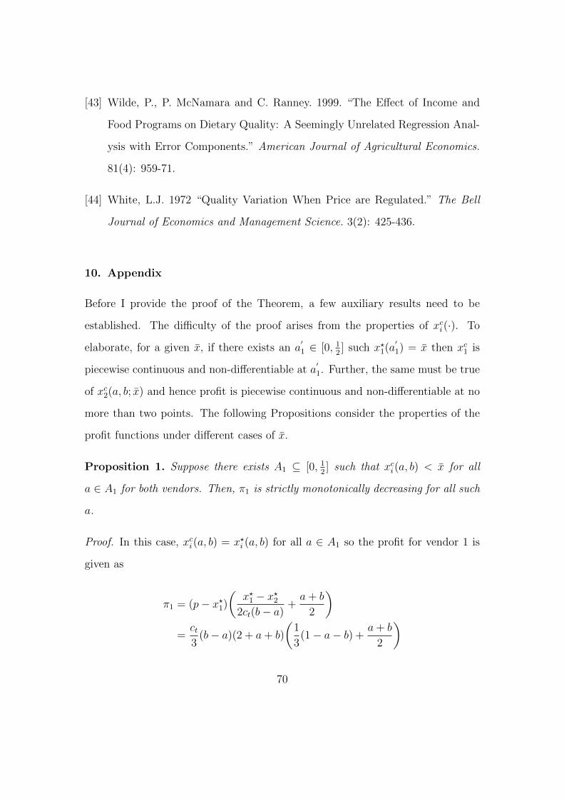
[43] Wilde, P., P. McNamara and C. Ranney. 1999. “The Effect of Income and

Food Programs on Dietary Quality: A Seemingly Unrelated Regression Anal-

ysis with Error Components.” American Journal of Agricultural Economics.

81(4): 959-71.

[44] White, L.J. 1972 “Quality Variation When Price are Regulated.” The Bell

Journal of Economics and Management Science. 3(2): 425-436.

10. Appendix

Before I provide the proof of the Theorem, a few auxiliary results need to be

established. The difficulty of the proof arises from the properties of xci(·). To

elaborate, for a given x̄, if there exists an a′1 ∈ [0, 1

2] such x?1(a

′1) = x̄ then xc1 is

piecewise continuous and non-differentiable at a′1. Further, the same must be true

of xc2(a, b; x̄) and hence profit is piecewise continuous and non-differentiable at no

more than two points. The following Propositions consider the properties of the

profit functions under different cases of x̄.

Proposition 1. Suppose there exists A1 ⊆ [0, 12] such that xci(a, b) < x̄ for all

a ∈ A1 for both vendors. Then, π1 is strictly monotonically decreasing for all such

a.

Proof. In this case, xci(a, b) = x?i (a, b) for all a ∈ A1 so the profit for vendor 1 is

given as

π1 = (p− x?1)

(x?1 − x?2

2ct(b− a)+a+ b

2

)=ct3

(b− a)(2 + a+ b)

(1

3(1− a− b) +

a+ b

2

)

70

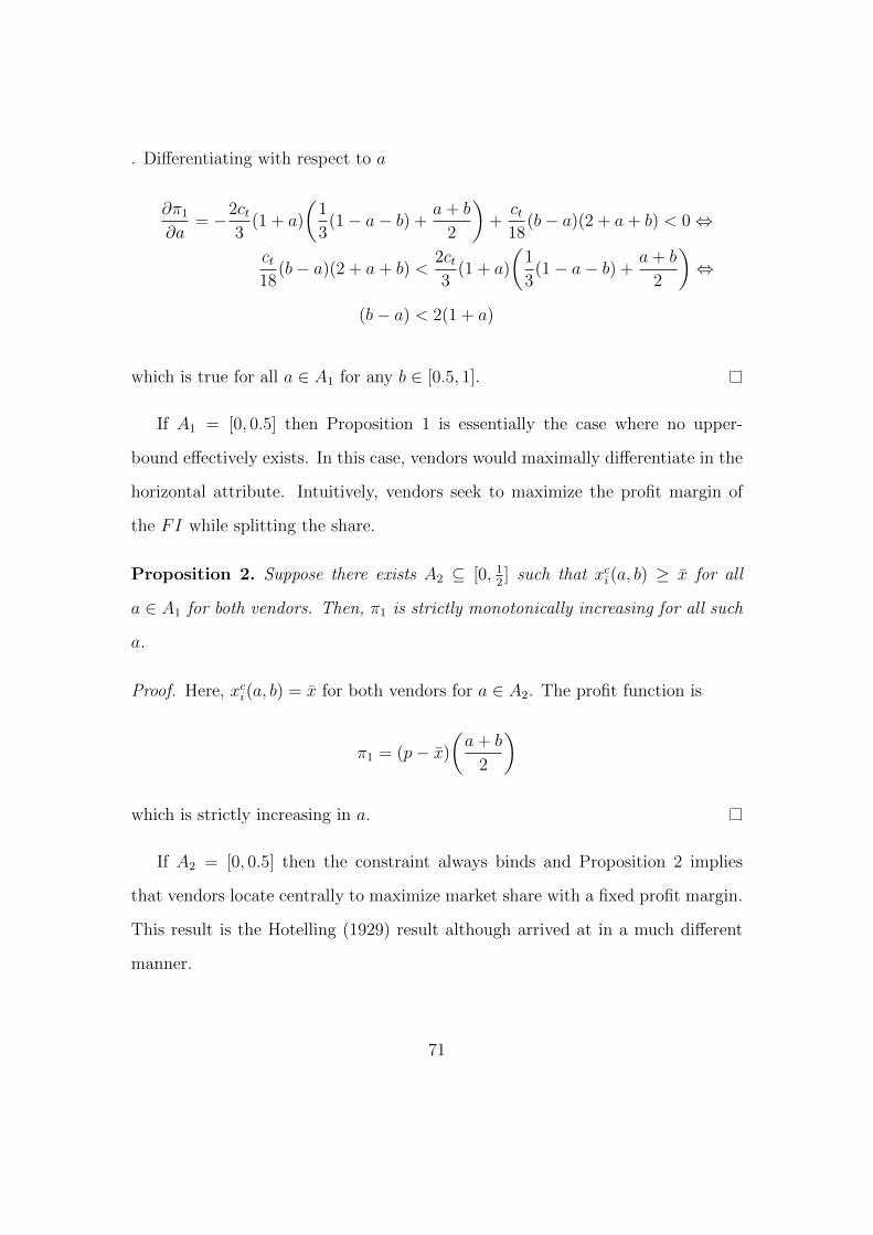
. Differentiating with respect to a

∂π1

∂a= −2ct

3(1 + a)

(1

3(1− a− b) +

a+ b

2

)+ct18

(b− a)(2 + a+ b) < 0⇔

ct18

(b− a)(2 + a+ b) <2ct3

(1 + a)

(1

3(1− a− b) +

a+ b

2

)⇔

(b− a) < 2(1 + a)

which is true for all a ∈ A1 for any b ∈ [0.5, 1].

If A1 = [0, 0.5] then Proposition 1 is essentially the case where no upper-

bound effectively exists. In this case, vendors would maximally differentiate in the

horizontal attribute. Intuitively, vendors seek to maximize the profit margin of

the FI while splitting the share.

Proposition 2. Suppose there exists A2 ⊆ [0, 12] such that xci(a, b) ≥ x̄ for all

a ∈ A1 for both vendors. Then, π1 is strictly monotonically increasing for all such

a.

Proof. Here, xci(a, b) = x̄ for both vendors for a ∈ A2. The profit function is

π1 = (p− x̄)

(a+ b

2

)

which is strictly increasing in a.

If A2 = [0, 0.5] then the constraint always binds and Proposition 2 implies

that vendors locate centrally to maximize market share with a fixed profit margin.

This result is the Hotelling (1929) result although arrived at in a much different

manner.

71

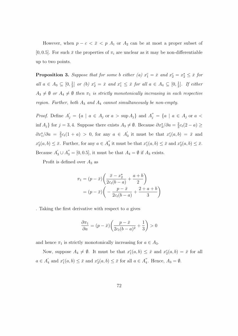
However, when p − c < x̄ < p A1 or A2 can be at most a proper subset of

[0, 0.5]. For such x̄ the properties of πi are unclear as it may be non-differentiable

up to two points.

Proposition 3. Suppose that for some b either (a) xc1 = x̄ and xc2 = x?2 ≤ x̄ for

all a ∈ A3 ⊆ [0, 12] or (b) xc2 = x̄ and xc1 ≤ x̄ for all a ∈ A4 ⊆ [0, 1

2]. If either

A3 6= ∅ or A4 6= ∅ then π1 is strictly monotonically increasing in each respective

region. Further, both A3 and A4 cannot simultaneously be non-empty.

Proof. Define A′j = {a | a ∈ Aj or a > supAj} and A

′′j = {a | a ∈ Aj or a <

inf Aj} for j = 3, 4. Suppose there exists A3 6= ∅. Because ∂x?2/∂a = 23ct(2− a) ≥

∂x?1/∂a = 23ct(1 + a) > 0, for any a ∈ A

′3 it must be that xc1(a, b) = x̄ and

xc2(a, b) ≤ x̄. Further, for any a ∈ A′′3 it must be that xc1(a, b) ≤ x̄ and xc2(a, b) ≤ x̄.

Because A′3 ∪ A

′′3 = [0, 0.5], it must be that A4 = ∅ if A3 exists.

Profit is defined over A3 as

π1 = (p− x̄)

(x̄− x?2

2ct(b− a)+a+ b

2

)= (p− x̄)

(− p− x̄

2ct(b− a)+

2 + a+ b

3

)

. Taking the first derivative with respect to a gives

∂π1

∂a= (p− x̄)

(p− x̄

2ct(b− a)2+

1

3

)> 0

and hence π1 is strictly monotonically increasing for a ∈ A3.

Now, suppose A4 6= ∅. It must be that xc1(a, b) ≤ x̄ and xc2(a, b) = x̄ for all

a ∈ A′4 and xc1(a, b) ≤ x̄ and xc2(a, b) ≤ x̄ for all a ∈ A′′

4 . Hence, A3 = ∅.

72

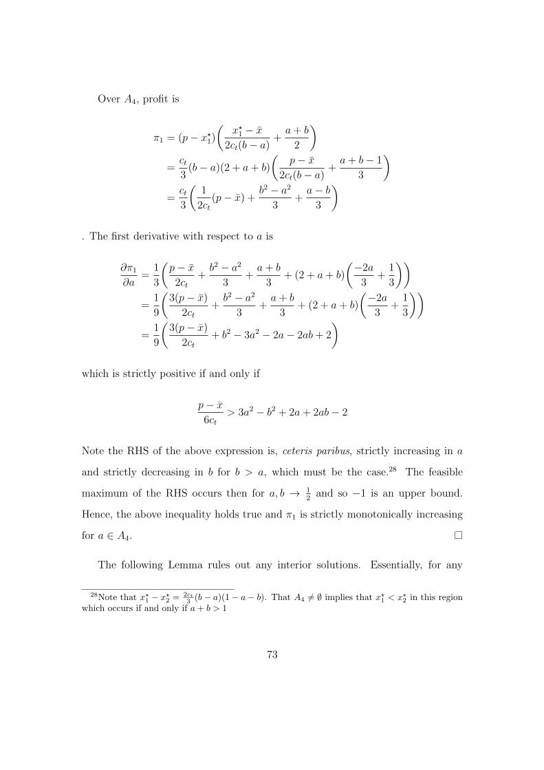
Over A4, profit is

π1 = (p− x?1)

(x?1 − x̄

2ct(b− a)+a+ b

2

)=ct3

(b− a)(2 + a+ b)

(p− x̄

2ct(b− a)+a+ b− 1

3

)=ct3

(1

2ct(p− x̄) +

b2 − a2

3+a− b

3

)

. The first derivative with respect to a is

∂π1

∂a=

1

3

(p− x̄2ct

+b2 − a2

3+a+ b

3+ (2 + a+ b)

(−2a

3+

1

3

))=

1

9

(3(p− x̄)

2ct+b2 − a2

3+a+ b

3+ (2 + a+ b)

(−2a

3+

1

3

))=

1

9

(3(p− x̄)

2ct+ b2 − 3a2 − 2a− 2ab+ 2

)

which is strictly positive if and only if

p− x̄6ct

> 3a2 − b2 + 2a+ 2ab− 2

Note the RHS of the above expression is, ceteris paribus, strictly increasing in a

and strictly decreasing in b for b > a, which must be the case.28 The feasible

maximum of the RHS occurs then for a, b → 12

and so −1 is an upper bound.

Hence, the above inequality holds true and π1 is strictly monotonically increasing

for a ∈ A4.

The following Lemma rules out any interior solutions. Essentially, for any

28Note that x?1 − x?2 = 2ct3 (b− a)(1− a− b). That A4 6= ∅ implies that x?1 < x?2 in this region

which occurs if and only if a+ b > 1

73

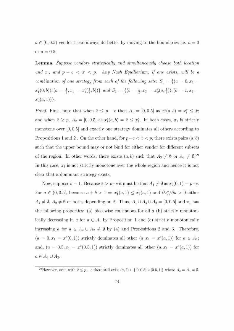
a ∈ (0, 0.5) vendor 1 can always do better by moving to the boundaries i.e. a = 0

or a = 0.5.

Lemma. Suppose vendors strategically and simultaneously choose both location

and xi, and p − c < x̄ < p. Any Nash Equilibrium, if one exists, will be a

combination of one strategy from each of the following sets: S1 = {(a = 0, x1 =

xc1(0, b)), (a = 12, x1 = xc1(1

2, b))} and S2 = {(b = 1

2, x2 = xc2(a, 1

2)), (b = 1, x2 =

xc2(a, 1))}.

Proof. First, note that when x̄ ≤ p − c then A1 = [0, 0.5] as xci(a, b) = x?i ≤ x̄;

and when x̄ ≥ p, A2 = [0, 0.5] as xci(a, b) = x̄ ≤ x?i . In both cases, π1 is strictly

monotone over [0, 0.5] and exactly one strategy dominates all others according to

Propositions 1 and 2 . On the other hand, for p−c < x̄ < p, there exists pairs (a, b)

such that the upper bound may or not bind for either vendor for different subsets

of the region. In other words, there exists (a, b) such that A3 6= ∅ or A4 6= ∅.29

In this case, π1 is not strictly monotone over the whole region and hence it is not

clear that a dominant strategy exists.

Now, suppose b = 1. Because x̄ > p−c it must be thatA1 6= ∅ as xci(0, 1) = p−c.

For a ∈ (0, 0.5], because a + b > 1 ⇒ xc1(a, 1) ≤ xc2(a, 1) and ∂x?i /∂a > 0 either

A4 6= ∅, A2 6= ∅ or both, depending on x̄. Thus, A1 ∪A4 ∪A2 = [0, 0.5] and π1 has

the following properties: (a) piecewise continuous for all a (b) strictly monoton-

ically decreasing in a for a ∈ A1 by Proposition 1 and (c) strictly monotonically

increasing a for a ∈ A4 ∪ A2 6= ∅ by (a) and Propositions 2 and 3. Therefore,

(a = 0, x1 = xc(0, 1)) strictly dominates all other (a, x1 = xc(a, 1)) for a ∈ A1;

and, (a = 0.5, x1 = xc(0.5, 1)) strictly dominates all other (a, x1 = xc(a, 1)) for

a ∈ A4 ∪ A2.

29However, even with x̄ ≤ p− c there still exist (a, b) ∈ {[0, 0.5]× [0.5, 1]} where A3 = A4 = ∅.

74

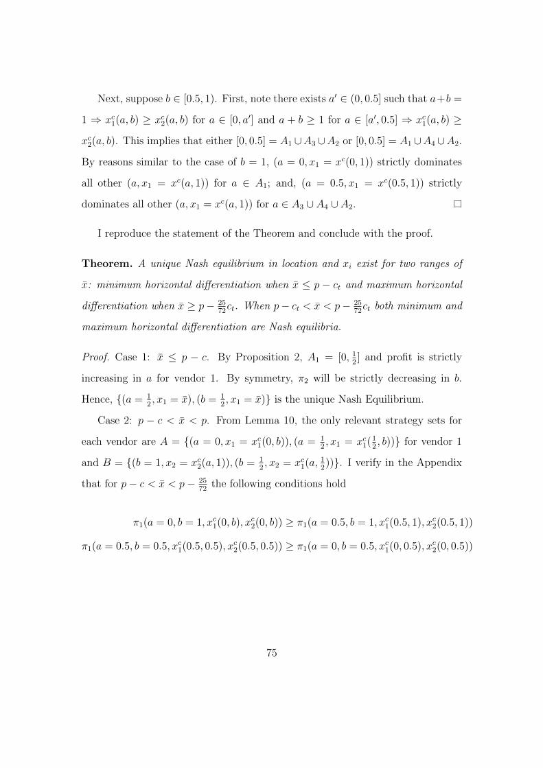
Next, suppose b ∈ [0.5, 1). First, note there exists a′ ∈ (0, 0.5] such that a+b =

1 ⇒ xc1(a, b) ≥ xc2(a, b) for a ∈ [0, a′] and a + b ≥ 1 for a ∈ [a′, 0.5] ⇒ xc1(a, b) ≥

xc2(a, b). This implies that either [0, 0.5] = A1 ∪A3 ∪A2 or [0, 0.5] = A1 ∪A4 ∪A2.

By reasons similar to the case of b = 1, (a = 0, x1 = xc(0, 1)) strictly dominates

all other (a, x1 = xc(a, 1)) for a ∈ A1; and, (a = 0.5, x1 = xc(0.5, 1)) strictly

dominates all other (a, x1 = xc(a, 1)) for a ∈ A3 ∪ A4 ∪ A2.

I reproduce the statement of the Theorem and conclude with the proof.

Theorem. A unique Nash equilibrium in location and xi exist for two ranges of

x̄: minimum horizontal differentiation when x̄ ≤ p − ct and maximum horizontal

differentiation when x̄ ≥ p− 2572ct. When p− ct < x̄ < p− 25

72ct both minimum and

maximum horizontal differentiation are Nash equilibria.

Proof. Case 1: x̄ ≤ p − c. By Proposition 2, A1 = [0, 12] and profit is strictly

increasing in a for vendor 1. By symmetry, π2 will be strictly decreasing in b.

Hence, {(a = 12, x1 = x̄), (b = 1

2, x1 = x̄)} is the unique Nash Equilibrium.

Case 2: p − c < x̄ < p. From Lemma 10, the only relevant strategy sets for

each vendor are A = {(a = 0, x1 = xc1(0, b)), (a = 12, x1 = xc1(1

2, b))} for vendor 1

and B = {(b = 1, x2 = xc2(a, 1)), (b = 12, x2 = xc1(a, 1

2))}. I verify in the Appendix

that for p− c < x̄ < p− 2572

the following conditions hold

π1(a = 0, b = 1, xc1(0, b), xc2(0, b)) ≥ π1(a = 0.5, b = 1, xc1(0.5, 1), xc2(0.5, 1))

π1(a = 0.5, b = 0.5, xc1(0.5, 0.5), xc2(0.5, 0.5)) ≥ π1(a = 0, b = 0.5, xc1(0, 0.5), xc2(0, 0.5))

75

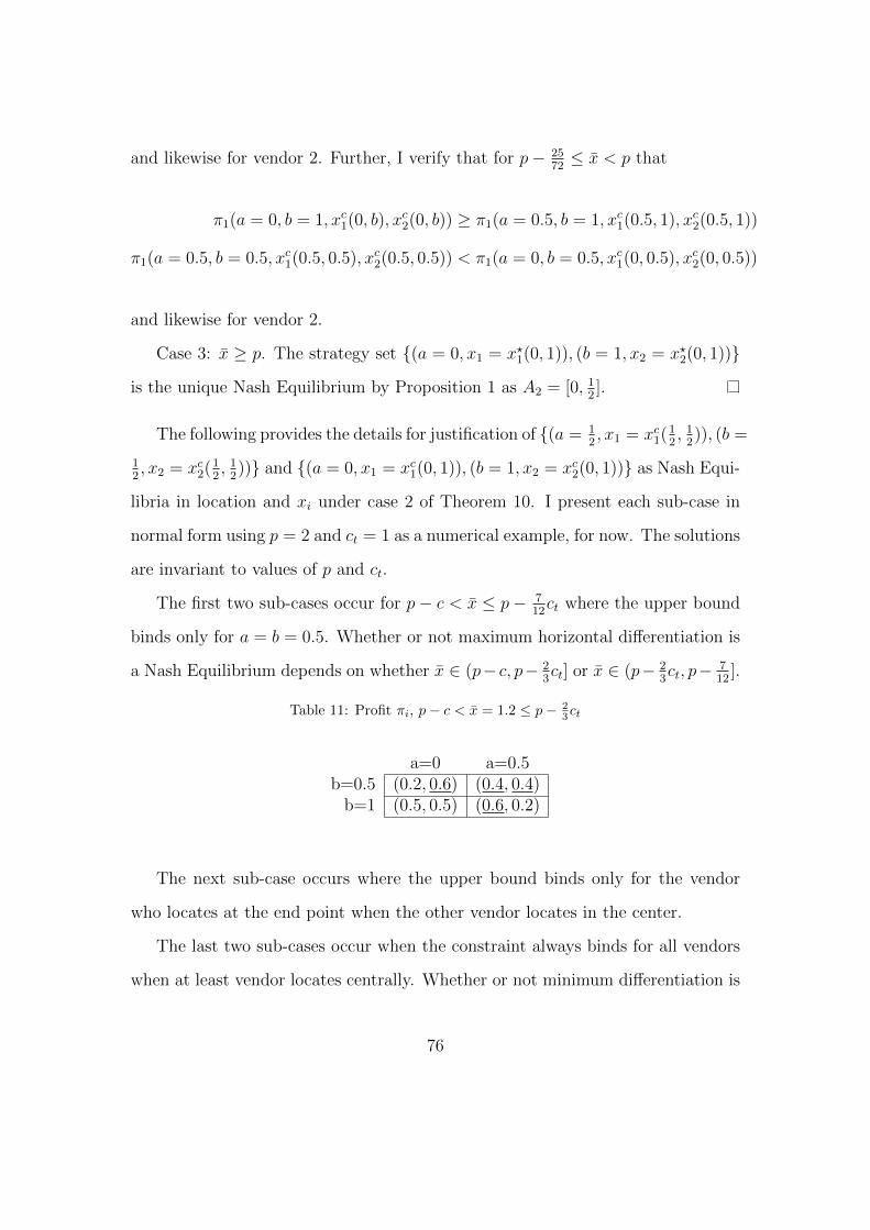
and likewise for vendor 2. Further, I verify that for p− 2572≤ x̄ < p that

π1(a = 0, b = 1, xc1(0, b), xc2(0, b)) ≥ π1(a = 0.5, b = 1, xc1(0.5, 1), xc2(0.5, 1))

π1(a = 0.5, b = 0.5, xc1(0.5, 0.5), xc2(0.5, 0.5)) < π1(a = 0, b = 0.5, xc1(0, 0.5), xc2(0, 0.5))

and likewise for vendor 2.

Case 3: x̄ ≥ p. The strategy set {(a = 0, x1 = x?1(0, 1)), (b = 1, x2 = x?2(0, 1))}

is the unique Nash Equilibrium by Proposition 1 as A2 = [0, 12].

The following provides the details for justification of {(a = 12, x1 = xc1(1

2, 1

2)), (b =

12, x2 = xc2(1

2, 1

2))} and {(a = 0, x1 = xc1(0, 1)), (b = 1, x2 = xc2(0, 1))} as Nash Equi-

libria in location and xi under case 2 of Theorem 10. I present each sub-case in

normal form using p = 2 and ct = 1 as a numerical example, for now. The solutions

are invariant to values of p and ct.

The first two sub-cases occur for p− c < x̄ ≤ p− 712ct where the upper bound

binds only for a = b = 0.5. Whether or not maximum horizontal differentiation is

a Nash Equilibrium depends on whether x̄ ∈ (p− c, p− 23ct] or x̄ ∈ (p− 2

3ct, p− 7

12].

Table 11: Profit πi, p− c < x̄ = 1.2 ≤ p− 23ct

a=0 a=0.5b=0.5 (0.2, 0.6) (0.4, 0.4)

b=1 (0.5, 0.5) (0.6, 0.2)

The next sub-case occurs where the upper bound binds only for the vendor

who locates at the end point when the other vendor locates in the center.

The last two sub-cases occur when the constraint always binds for all vendors

when at least vendor locates centrally. Whether or not minimum differentiation is

76

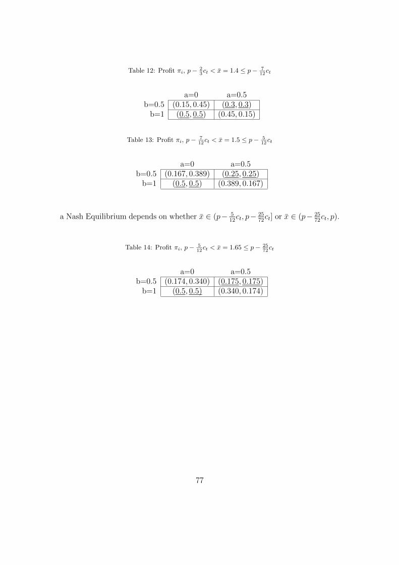
Table 12: Profit πi, p− 23ct < x̄ = 1.4 ≤ p− 7

12ct

a=0 a=0.5b=0.5 (0.15, 0.45) (0.3, 0.3)

b=1 (0.5, 0.5) (0.45, 0.15)


12ct

a=0 a=0.5b=0.5 (0.167, 0.389) (0.25, 0.25)

b=1 (0.5, 0.5) (0.389, 0.167)

a Nash Equilibrium depends on whether x̄ ∈ (p− 512ct, p− 25

72ct] or x̄ ∈ (p− 25

72ct, p).


72ct

a=0 a=0.5b=0.5 (0.174, 0.340) (0.175, 0.175)

b=1 (0.5, 0.5) (0.340, 0.174)

77

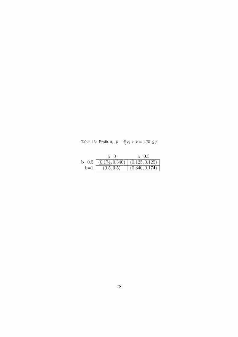
Table 15: Profit πi, p− 2572ct < x̄ = 1.75 ≤ p

a=0 a=0.5b=0.5 (0.174, 0.340) (0.125, 0.125)

b=1 (0.5, 0.5) (0.340, 0.174)

78

Incentives for Non-Price Competition in the California WIC Program Job Market … · 2014-10-08 ·...

Documents

Transcript of Incentives for Non-Price Competition in the California WIC Program Job Market … · 2014-10-08 ·...