vsm tutorial

COPYRIGHT NOTICE

© Labcenter Electronics Ltd 1990-2011. All Rights Reserved. The PROTEUS software programs (ISIS, PROSPICE and ARES) and their associated library files, data files and documentation are copyright © Labcenter Electronics Ltd. All rights reserved. You have bought a licence to use the software on one machine at any one time; you do not own the software. Unauthorized copying, lending, or re-distribution of the software or documentation in any manner constitutes breach of copyright. Software piracy is theft.

PROSPICE incorporates source code from Berkeley SPICE3F5 which is copyright © Regents of Berkeley University. Manufacturer’s SPICE models included with the software are copyright of their respective originators.

WARNING You may make a single copy of the software for backup purposes. However, you are warned that the software contains an encrypted serialization system. Any given copy of the software is therefore traceable to the master disk supplied with your licence.

PROTEUS also contains special code that will prevent more that one copy using a particular licence key on a network at any given time. Therefore, you must purchase a licence key for each copy that you want to run simultaneously.

DISCLAIMER No warranties of any kind are made with respect to the contents of this software package, nor its fitness for any particular purpose. Neither Labcenter Electronics Ltd nor any of its employees or sub-contractors shall be liable for errors in the software, component libraries, simulator models or documentation, or for any direct, indirect or consequential damages or financial losses arising from the use of the package.

Users are particularly reminded that successful simulation of a design with the PROSPICE simulator does not prove conclusively that it will work when manufactured. It is always best to make a one off prototype before having large numbers of boards produced.

Manufacturers’ SPICE models included with PROSPICE are supplied on an ‘as-is’ basis and neither Labcenter nor their originators make any warranty whatsoever as to their accuracy or functionality

TABLE OF CONTENTS

COPYRIGHT NOTICE ................................................................................................................... 1

© Labcenter Electronics Ltd 1990-2010. All Rights Reserved. ................................................. 1

WARNING .................................................................................................................................. 1

DISCLAIMER ............................................................................................................................. 1

TABLE OF CONTENTS ................................................................................................................ 1

INTRODUCTION ........................................................................................................................... 1

INTERACTIVE TUTORIAL ........................................................................................................... 3

Overview .................................................................................................................................... 3

Requirements: ........................................................................................................................ 4

Project Setup ............................................................................................................................. 5

Further Reading: .................................................................................................................... 7

Compile and Run ....................................................................................................................... 8

Further Reading: .................................................................................................................... 9

Writing Firmware ...................................................................................................................... 10

Basic Debugging ...................................................................................................................... 15

Important Points: .................................................................................................................. 17

The Watch Window .................................................................................................................. 18

Hardware Breakpoints ............................................................................................................. 22

Interactive Measurements........................................................................................................ 24

Further Reading: .................................................................................................................. 26

Graph Based Measurements ................................................................................................... 27

Further Reading: .................................................................................................................. 32

Diagnostic Messaging .............................................................................................................. 33

GRAPH BASED TUTORIAL ....................................................................................................... 36

Introduction .............................................................................................................................. 36

Getting Started ......................................................................................................................... 36

Generators ............................................................................................................................... 37

Probes ...................................................................................................................................... 39

Graphs ...................................................................................................................................... 39

Simulation ................................................................................................................................. 41

Taking Measurements .............................................................................................................. 42

Using Current Probes ............................................................................................................... 44

Frequency Analysis .................................................................................................................. 44

Swept Variable Analysis ........................................................................................................... 45

Noise Analysis .......................................................................................................................... 46

1

INTRODUCTION The aim of this guide is to cover in brief the basic principles of microcontroller and graph based simulation with Proteus VSM. Typically, we will cover the basic principles here with more detailed information being available in the appropriate reference manual.

All of the reference manuals are included in HTMLHelp format with the software and can be accessed either from the start menu or from the Help Menu in the applications. The reference manuals also include many topics not covered at all in this getting started guide.

You will also find that each dialogue form in the Proteus software has specific help associated with it. Help on a dialogue form can be launched by clicking on the question mark at the top right of the dialogue form and then on a particular field of the dialogue.

You may also find our web based support forums useful for general Proteus enquiries and discussion : http://support.labcenter.co.uk

Finally, if you still have questions or problems after consulting the reference manual please contact your local authorized distributor for technical support or mail us directly at [email protected] quoting your customer number in the subject line of the email.

http://support.labcenter.co.uk/

mailto:[email protected]

LABCENTER ELECTRONICS LTD.

2

3

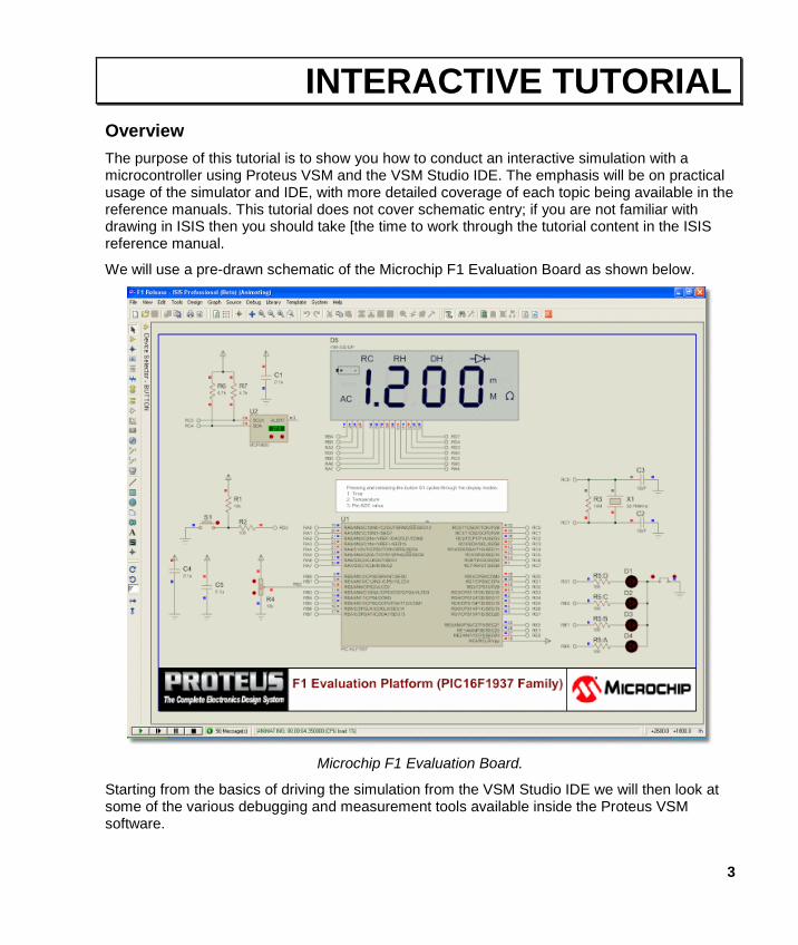
INTERACTIVE TUTORIAL Overview The purpose of this tutorial is to show you how to conduct an interactive simulation with a microcontroller using Proteus VSM and the VSM Studio IDE. The emphasis will be on practical usage of the simulator and IDE, with more detailed coverage of each topic being available in the reference manuals. This tutorial does not cover schematic entry; if you are not familiar with drawing in ISIS then you should take [the time to work through the tutorial content in the ISIS reference manual.

We will use a pre-drawn schematic of the Microchip F1 Evaluation Board as shown below.

Microchip F1 Evaluation Board.

Starting from the basics of driving the simulation from the VSM Studio IDE we will then look at some of the various debugging and measurement tools available inside the Proteus VSM software.


4

Requirements:

To work through this tutorial you will need :

• An installed copy of the VSM Studio IDE. This can be downloaded free of charge from the Labcenter website (http://www.labcenter.com).

• An installed copy of the Proteus Software at Version 7.8 or later. A demonstration copy of the software can be downloaded free of charge from the Labcenter website if you do not have a professional copy.

• An installed copy of the Hi-Tech PIC16 compiler at Version 9.8 or later. A free (Lite) copy of this can be downloaded from the Microchip website.

We would still recommend you read through the tutorial, even if you do not have the tools installed. Most of the material - and all of the debugging techniques - are generic and will prove useful in your own designs.

If you choose not to use the VSM Studio IDE then the section of the Proteus VSM Reference Manual entitled ‘Supported Debug Formats’ is critical reading. Once you understand this, all of the debugging tools discussed in this tutorial will be available.

PROTEUS VSM

5

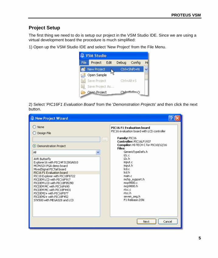
Project Setup The first thing we need to do is setup our project in the VSM Studio IDE. Since we are using a virtual development board the procedure is much simplified:

1) Open up the VSM Studio IDE and select 'New Project' from the File Menu.

2) Select 'PIC16F1 Evaluation Board' from the 'Demonstration Projects' and then click the next button.


6

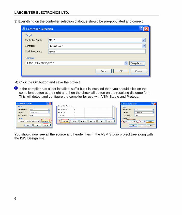
3) Everything on the controller selection dialogue should be pre-populated and correct.

4) Click the OK button and save the project.

If the compiler has a 'not installed' suffix but it is installed then you should click on the compilers button at the right and then the check all button on the resulting dialogue form. This will detect and configure the compiler for use with VSM Studio and Proteus.

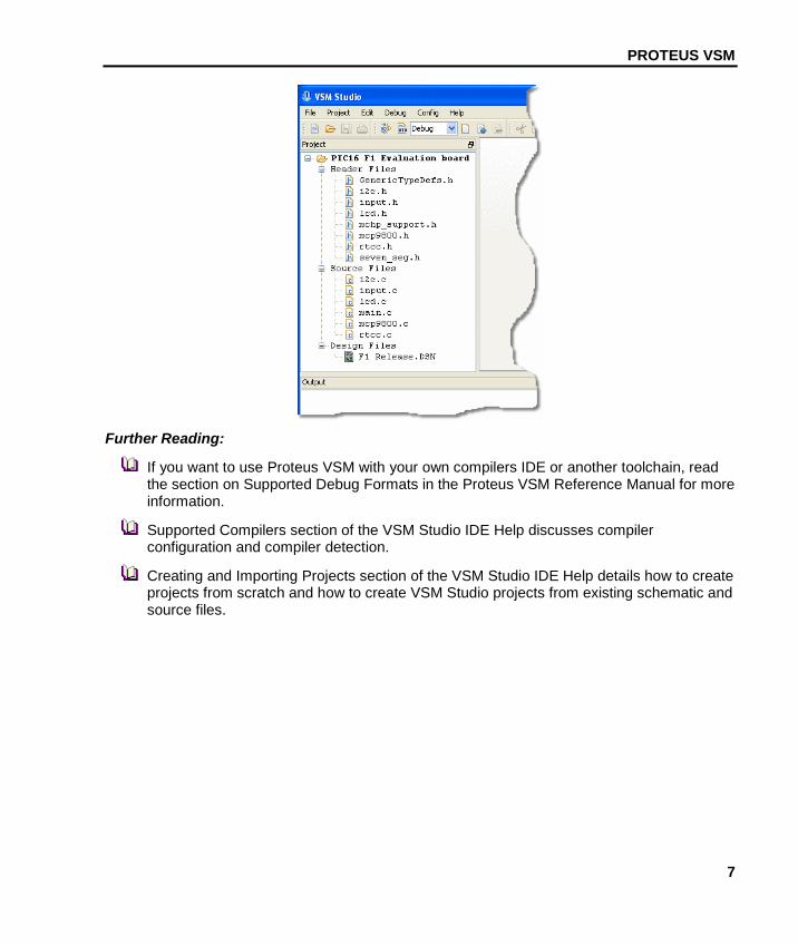
You should now see all the source and header files in the VSM Studio project tree along with the ISIS Design File.

PROTEUS VSM

7

Further Reading:

If you want to use Proteus VSM with your own compilers IDE or another toolchain, read the section on Supported Debug Formats in the Proteus VSM Reference Manual for more information.

Supported Compilers section of the VSM Studio IDE Help discusses compiler configuration and compiler detection.

Creating and Importing Projects section of the VSM Studio IDE Help details how to create projects from scratch and how to create VSM Studio projects from existing schematic and source files.


8

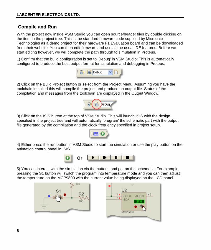
Compile and Run With the project now inside VSM Studio you can open source/header files by double clicking on the item in the project tree. This is the standard firmware code supplied by Microchip Technologies as a demo project for their hardware F1 Evaluation board and can be downloaded from their website. You can then edit firmware and use all the usual IDE features. Before we start editing however, we will complete the path through to simulation in Proteus.

1) Confirm that the build configuration is set to 'Debug' in VSM Studio; This is automatically configured to produce the best output format for simulation and debugging in Proteus.

2) Click on the Build Project button or select from the Project Menu. Assuming you have the toolchain installed this will compile the project and produce an output file. Status of the compilation and messages from the toolchain are displayed in the Output Window.

3) Click on the ISIS button at the top of VSM Studio. This will launch ISIS with the design specified in the project tree and will automatically 'program' the schematic part with the output file generated by the compilation and the clock frequency specified in project setup.

4) Either press the run button in VSM Studio to start the simulation or use the play button on the animation control panel in ISIS.

5) You can interact with the simulation via the buttons and pot on the schematic. For example, pressing the S1 button will switch the program into temperature mode and you can then adjust the temperature on the MCP9800 with the current value being displayed on the LCD panel.

PROTEUS VSM

9

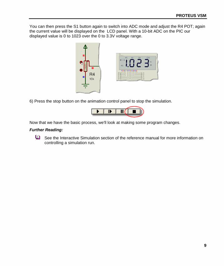
You can then press the S1 button again to switch into ADC mode and adjust the R4 POT; again the current value will be displayed on the LCD panel. With a 10-bit ADC on the PIC our displayed value is 0 to 1023 over the 0 to 3.3V voltage range.

6) Press the stop button on the animation control panel to stop the simulation.

Now that we have the basic process, we'll look at making some program changes.

Further Reading:

See the Interactive Simulation section of the reference manual for more information on controlling a simulation run.


10

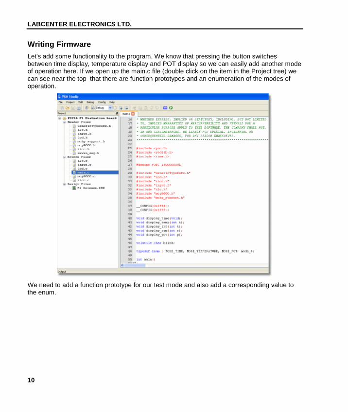
Writing Firmware Let's add some functionality to the program. We know that pressing the button switches between time display, temperature display and POT display so we can easily add another mode of operation here. If we open up the main.c file (double click on the item in the Project tree) we can see near the top that there are function prototypes and an enumeration of the modes of operation.

We need to add a function prototype for our test mode and also add a corresponding value to the enum.

PROTEUS VSM

11

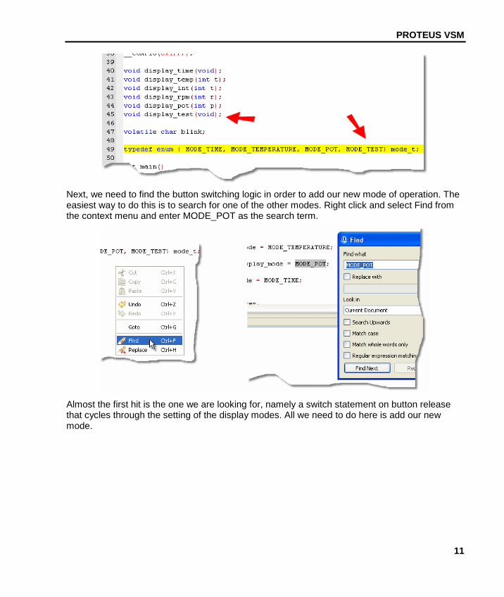
Next, we need to find the button switching logic in order to add our new mode of operation. The easiest way to do this is to search for one of the other modes. Right click and select Find from the context menu and enter MODE_POT as the search term.

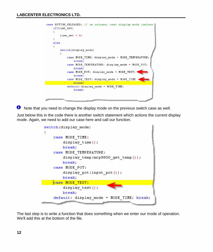
Almost the first hit is the one we are looking for, namely a switch statement on button release that cycles through the setting of the display modes. All we need to do here is add our new mode.


12

Note that you need to change the display mode on the previous switch case as well.

Just below this in the code there is another switch statement which actions the current display mode. Again, we need to add our case here and call our function.

The last step is to write a function that does something when we enter our mode of operation. We'll add this at the bottom of the file.

PROTEUS VSM

13

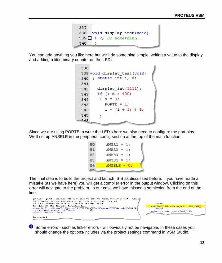
You can add anything you like here but we'll do something simple, writing a value to the display and adding a little binary counter on the LED's:

Since we are using PORTE to write the LED's here we also need to configure the port pins. We'll set up ANSELE in the peripheral config section at the top of the main function.

The final step is to build the project and launch ISIS as discussed before. If you have made a mistake (as we have here) you will get a compiler error in the output window. Clicking on this error will navigate to the problem. In our case we have missed a semicolon from the end of the line.

Some errors - such as linker errors - will obviously not be navigable. In these cases you should change the options/includes via the project settings command in VSM Studio.


14

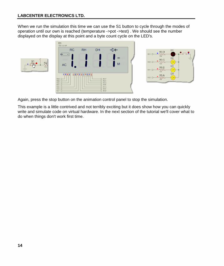
When we run the simulation this time we can use the S1 button to cycle through the modes of operation until our own is reached (temperature ->pot ->test) . We should see the number displayed on the display at this point and a byte count cycle on the LED's.

Again, press the stop button on the animation control panel to stop the simulation.

This example is a little contrived and not terribly exciting but it does show how you can quickly write and simulate code on virtual hardware. In the next section of the tutorial we'll cover what to do when things don't work first time.

PROTEUS VSM

15

Basic Debugging Much of the real power of using Proteus VSM comes from it's debugging capabilities. We have already seen how we can write code and test during free running simulation and we'll now look at how to step through our code in simulation time.

1) Start the simulation in ISIS with the pause button on the animation control panel.

2) You should notice that the simulation reports that it is paused at time zero and that a source window and a variables window have appeared.

At this stage the simulation has 'booted' and a stable operating point has been found but no instructions have executed and no real time has elapsed. The source window will not show any file as there is no source line at the current program counter value.

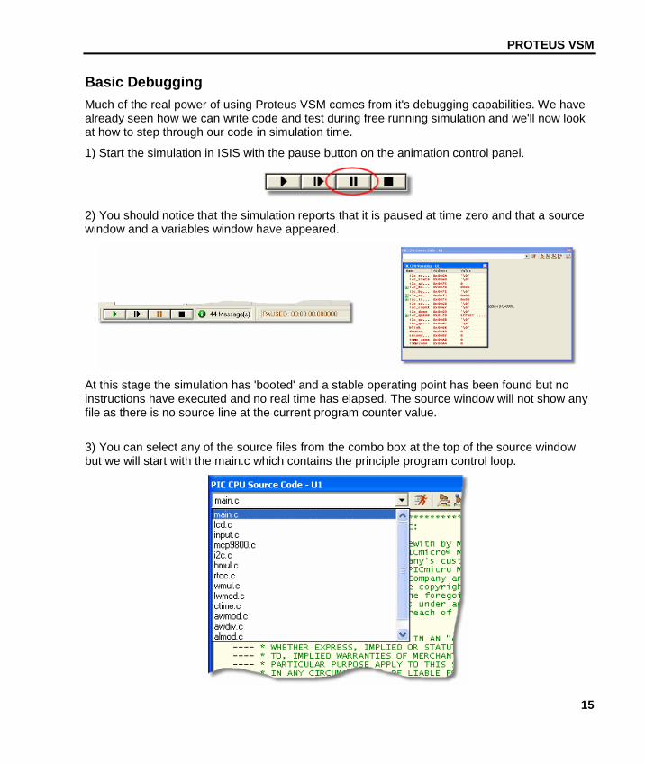
3) You can select any of the source files from the combo box at the top of the source window but we will start with the main.c which contains the principle program control loop.


16

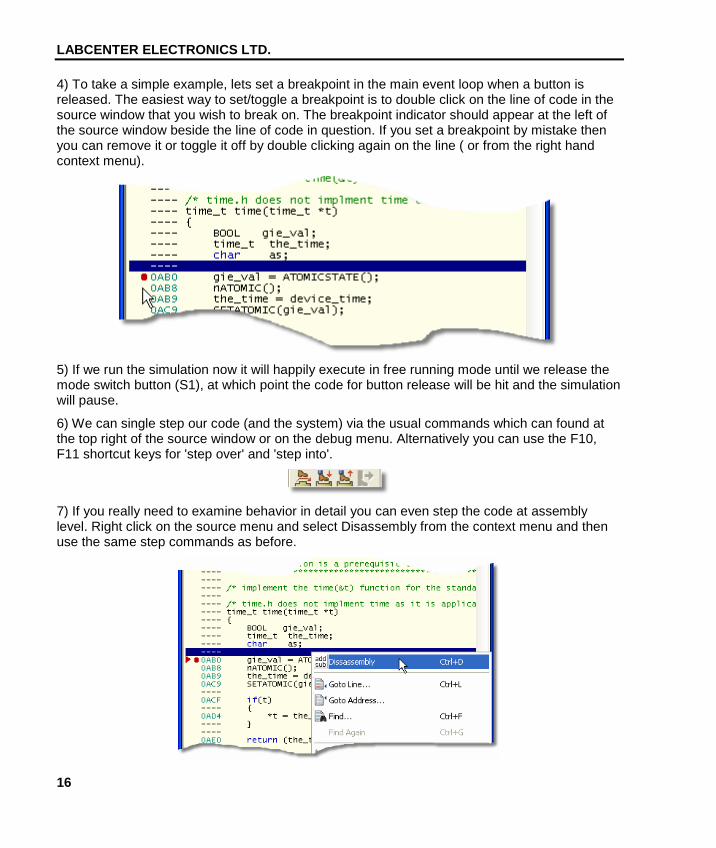
4) To take a simple example, lets set a breakpoint in the main event loop when a button is released. The easiest way to set/toggle a breakpoint is to double click on the line of code in the source window that you wish to break on. The breakpoint indicator should appear at the left of the source window beside the line of code in question. If you set a breakpoint by mistake then you can remove it or toggle it off by double clicking again on the line ( or from the right hand context menu).

5) If we run the simulation now it will happily execute in free running mode until we release the mode switch button (S1), at which point the code for button release will be hit and the simulation will pause.

6) We can single step our code (and the system) via the usual commands which can found at the top right of the source window or on the debug menu. Alternatively you can use the F10, F11 shortcut keys for 'step over' and 'step into'.

7) If you really need to examine behavior in detail you can even step the code at assembly level. Right click on the source menu and select Disassembly from the context menu and then use the same step commands as before.

PROTEUS VSM

17

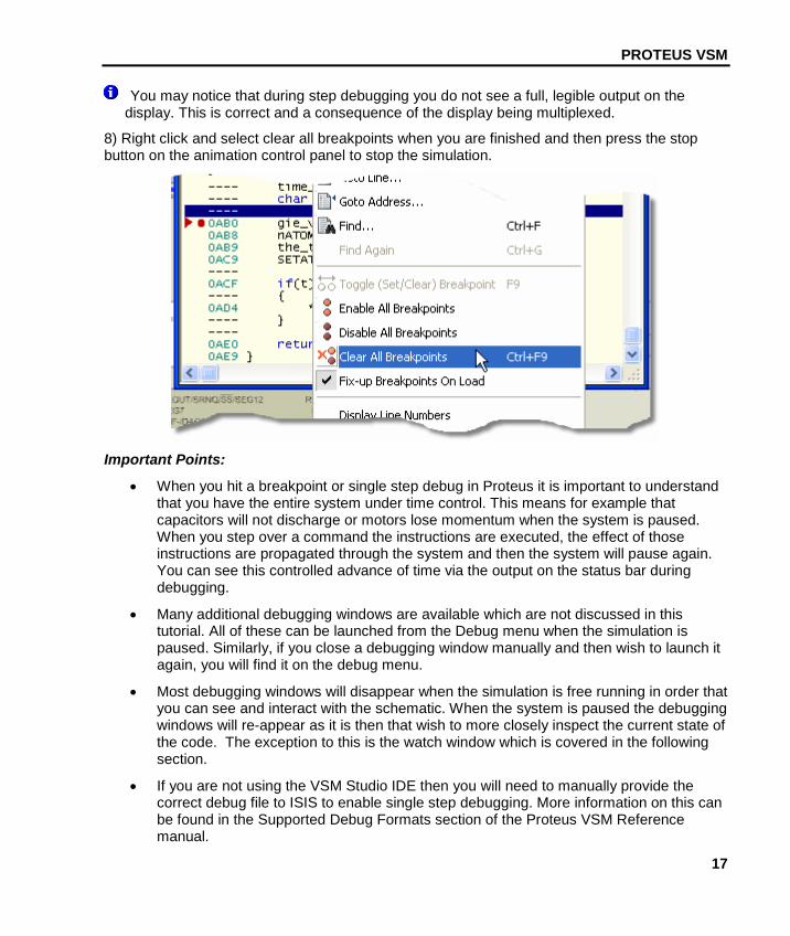
You may notice that during step debugging you do not see a full, legible output on the display. This is correct and a consequence of the display being multiplexed.

8) Right click and select clear all breakpoints when you are finished and then press the stop button on the animation control panel to stop the simulation.

Important Points:

• When you hit a breakpoint or single step debug in Proteus it is important to understand that you have the entire system under time control. This means for example that capacitors will not discharge or motors lose momentum when the system is paused. When you step over a command the instructions are executed, the effect of those instructions are propagated through the system and then the system will pause again. You can see this controlled advance of time via the output on the status bar during debugging.

• Many additional debugging windows are available which are not discussed in this tutorial. All of these can be launched from the Debug menu when the simulation is paused. Similarly, if you close a debugging window manually and then wish to launch it again, you will find it on the debug menu.

• Most debugging windows will disappear when the simulation is free running in order that you can see and interact with the schematic. When the system is paused the debugging windows will re-appear as it is then that wish to more closely inspect the current state of the code. The exception to this is the watch window which is covered in the following section.

• If you are not using the VSM Studio IDE then you will need to manually provide the correct debug file to ISIS to enable single step debugging. More information on this can be found in the Supported Debug Formats section of the Proteus VSM Reference manual.


18

The Watch Window The watch window is the one debugging window that remains open during free running simulation and it also gives us a different way to target breakpoints. To start with, lets use the watch window to monitor the ADC conversions from the POT.

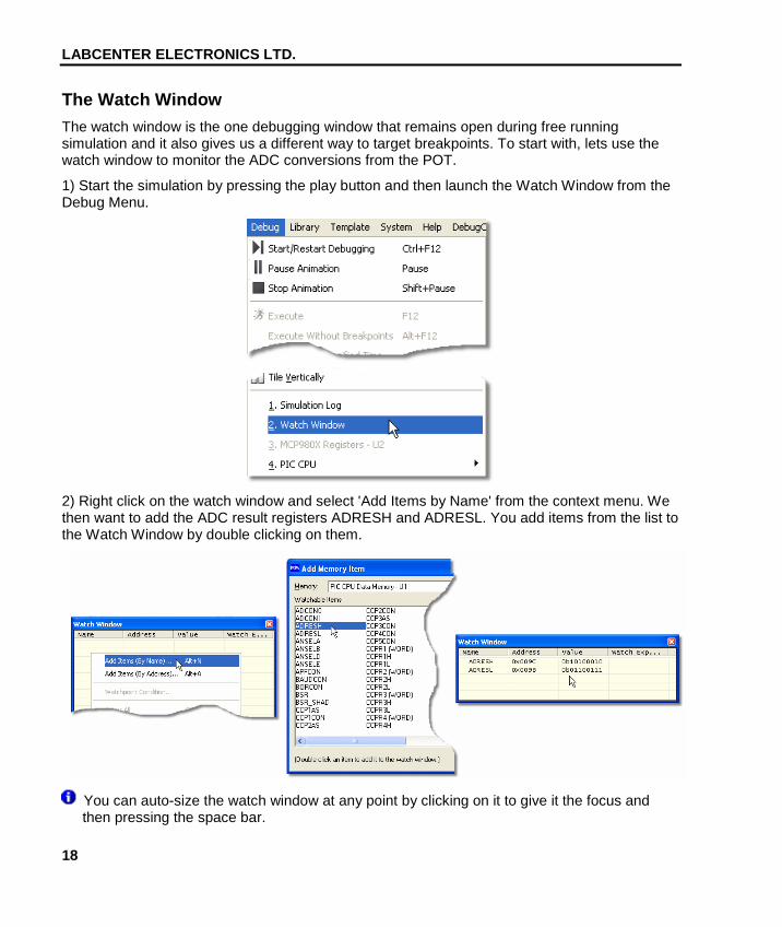
1) Start the simulation by pressing the play button and then launch the Watch Window from the Debug Menu.

2) Right click on the watch window and select 'Add Items by Name' from the context menu. We then want to add the ADC result registers ADRESH and ADRESL. You add items from the list to the Watch Window by double clicking on them.

You can auto-size the watch window at any point by clicking on it to give it the focus and then pressing the space bar.

PROTEUS VSM

19

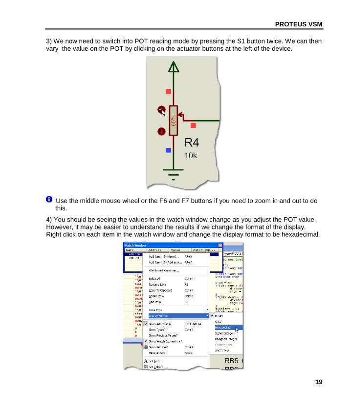
3) We now need to switch into POT reading mode by pressing the S1 button twice. We can then vary the value on the POT by clicking on the actuator buttons at the left of the device.

Use the middle mouse wheel or the F6 and F7 buttons if you need to zoom in and out to do this.

4) You should be seeing the values in the watch window change as you adjust the POT value. However, it may be easier to understand the results if we change the format of the display. Right click on each item in the watch window and change the display format to be hexadecimal.


20

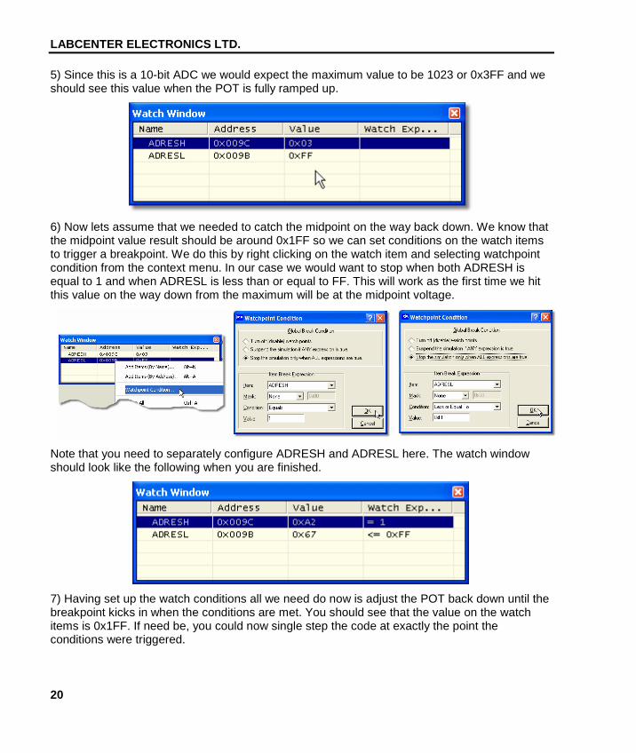
5) Since this is a 10-bit ADC we would expect the maximum value to be 1023 or 0x3FF and we should see this value when the POT is fully ramped up.

6) Now lets assume that we needed to catch the midpoint on the way back down. We know that the midpoint value result should be around 0x1FF so we can set conditions on the watch items to trigger a breakpoint. We do this by right clicking on the watch item and selecting watchpoint condition from the context menu. In our case we would want to stop when both ADRESH is equal to 1 and when ADRESL is less than or equal to FF. This will work as the first time we hit this value on the way down from the maximum will be at the midpoint voltage.

Note that you need to separately configure ADRESH and ADRESL here. The watch window should look like the following when you are finished.

7) Having set up the watch conditions all we need do now is adjust the POT back down until the breakpoint kicks in when the conditions are met. You should see that the value on the watch items is 0x1FF. If need be, you could now single step the code at exactly the point the conditions were triggered.

PROTEUS VSM

21

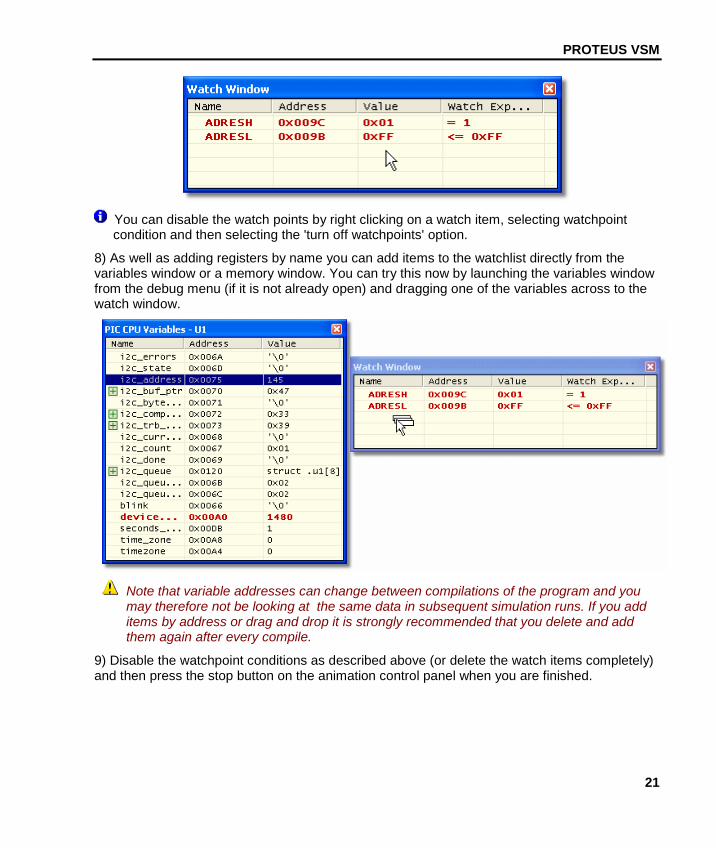
You can disable the watch points by right clicking on a watch item, selecting watchpoint condition and then selecting the 'turn off watchpoints' option.

8) As well as adding registers by name you can add items to the watchlist directly from the variables window or a memory window. You can try this now by launching the variables window from the debug menu (if it is not already open) and dragging one of the variables across to the watch window.

Note that variable addresses can change between compilations of the program and you may therefore not be looking at the same data in subsequent simulation runs. If you add items by address or drag and drop it is strongly recommended that you delete and add them again after every compile.

9) Disable the watchpoint conditions as described above (or delete the watch items completely) and then press the stop button on the animation control panel when you are finished.


22

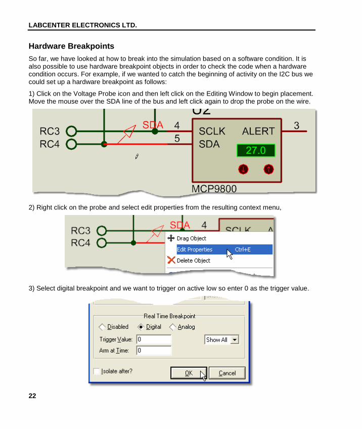
Hardware Breakpoints So far, we have looked at how to break into the simulation based on a software condition. It is also possible to use hardware breakpoint objects in order to check the code when a hardware condition occurs. For example, if we wanted to catch the beginning of activity on the I2C bus we could set up a hardware breakpoint as follows:

1) Click on the Voltage Probe icon and then left click on the Editing Window to begin placement. Move the mouse over the SDA line of the bus and left click again to drop the probe on the wire.

2) Right click on the probe and select edit properties from the resulting context menu,

3) Select digital breakpoint and we want to trigger on active low so enter 0 as the trigger value.

PROTEUS VSM

23

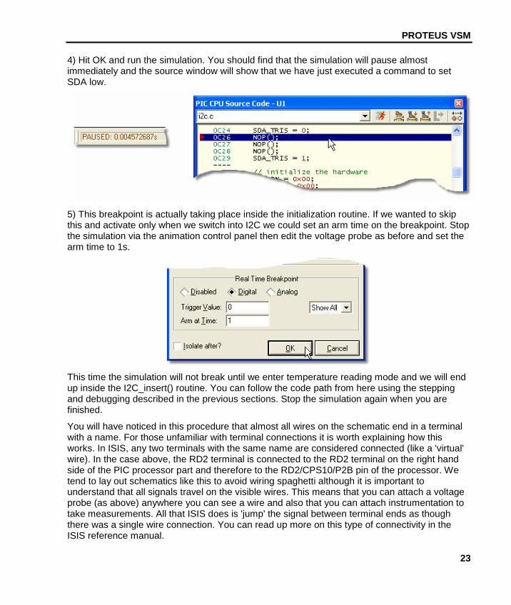
4) Hit OK and run the simulation. You should find that the simulation will pause almost immediately and the source window will show that we have just executed a command to set SDA low.

5) This breakpoint is actually taking place inside the initialization routine. If we wanted to skip this and activate only when we switch into I2C we could set an arm time on the breakpoint. Stop the simulation via the animation control panel then edit the voltage probe as before and set the arm time to 1s.

This time the simulation will not break until we enter temperature reading mode and we will end up inside the I2C_insert() routine. You can follow the code path from here using the stepping and debugging described in the previous sections. Stop the simulation again when you are finished.

You will have noticed in this procedure that almost all wires on the schematic end in a terminal with a name. For those unfamiliar with terminal connections it is worth explaining how this works. In ISIS, any two terminals with the same name are considered connected (like a 'virtual' wire). In the case above, the RD2 terminal is connected to the RD2 terminal on the right hand side of the PIC processor part and therefore to the RD2/CPS10/P2B pin of the processor. We tend to lay out schematics like this to avoid wiring spaghetti although it is important to understand that all signals travel on the visible wires. This means that you can attach a voltage probe (as above) anywhere you can see a wire and also that you can attach instrumentation to take measurements. All that ISIS does is 'jump' the signal between terminal ends as though there was a single wire connection. You can read up more on this type of connectivity in the ISIS reference manual.


24

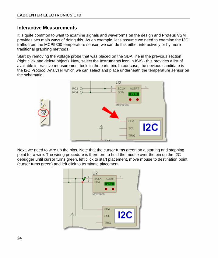
Interactive Measurements It is quite common to want to examine signals and waveforms on the design and Proteus VSM provides two main ways of doing this. As an example, let's assume we need to examine the I2C traffic from the MCP9800 temperature sensor; we can do this either interactively or by more traditional graphing methods.

Start by removing the voltage probe that was placed on the SDA line in the previous section (right click and delete object). Now, select the Instruments icon in ISIS - this provides a list of available interactive measurement tools in the parts bin. In our case, the obvious candidate is the I2C Protocol Analyser which we can select and place underneath the temperature sensor on the schematic.

Next, we need to wire up the pins. Note that the cursor turns green on a starting and stopping point for a wire. The wiring procedure is therefore to hold the mouse over the pin on the I2C debugger until cursor turns green, left click to start placement, move mouse to destination point (cursor turns green) and left click to terminate placement.

PROTEUS VSM

25

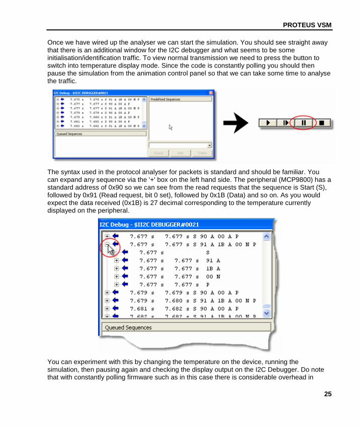
Once we have wired up the analyser we can start the simulation. You should see straight away that there is an additional window for the I2C debugger and what seems to be some initialisation/identification traffic. To view normal transmission we need to press the button to switch into temperature display mode. Since the code is constantly polling you should then pause the simulation from the animation control panel so that we can take some time to analyse the traffic.

The syntax used in the protocol analyser for packets is standard and should be familiar. You can expand any sequence via the '+' box on the left hand side. The peripheral (MCP9800) has a standard address of 0x90 so we can see from the read requests that the sequence is Start (S), followed by 0x91 (Read request, bit 0 set), followed by 0x1B (Data) and so on. As you would expect the data received (0x1B) is 27 decimal corresponding to the temperature currently displayed on the peripheral.

You can experiment with this by changing the temperature on the device, running the simulation, then pausing again and checking the display output on the I2C Debugger. Do note that with constantly polling firmware such as in this case there is considerable overhead in


26

terms of performance as we are constantly writing textual data to the display. However, in most cases you are using the instrument it is for testing or debugging, at which point the simulation speed is secondary to problem solving.

Further Reading:

More information on the I2C Protocol Analyser - along with other instrumentation - is available in the Proteus VSM reference manual. In particular, note that you can use the analyser as an I2C master device as well as simply a monitor.

More information on picking, placing and wiring in ISIS can be found in the ISIS Tutorial documentation.

PROTEUS VSM

27

Graph Based Measurements We can look at the same traffic in a different way by using graph based simulation. There are however some important differences which affect how we set up the simulation, namely:

• You cannot interact with the circuit during a graph based simulation.

• A graph based simulation runs for a specified period of time.

• The results are not visible until this period of time has finished and the simulation has stopped.

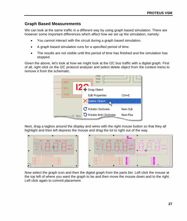
Given the above, let's look at how we might look at the I2C bus traffic with a digital graph. First of all, right click on the I2C protocol analyser and select delete object from the context menu to remove it from the schematic.

Next, drag a tagbox around the display and wires with the right mouse button so that they all highlight and then left depress the mouse and drag the lot to right out of the way.

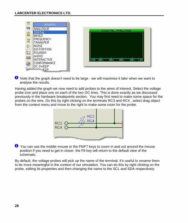
Now select the graph icon and then the digital graph from the parts bin. Left click the mouse at the top left of where you want the graph to be and then move the mouse down and to the right. Left click again to commit placement.


28

Note that the graph doesn't need to be large - we will maximise it later when we want to analyse the results.

Having added the graph we now need to add probes to the wires of interest. Select the voltage probe icon and place one on each of the two I2C lines. This is done exactly as we discussed previously in the hardware breakpoints section. You may first need to make some space for the probes on the wire. Do this by right clicking on the terminals RC3 and RC4 , select drag object from the context menu and move to the right to make some room for the probe.

You can use the middle mouse or the F6/F7 keys to zoom in and out around the mouse position if you need to get in closer. the F8 key will return to the default view of the schematic.

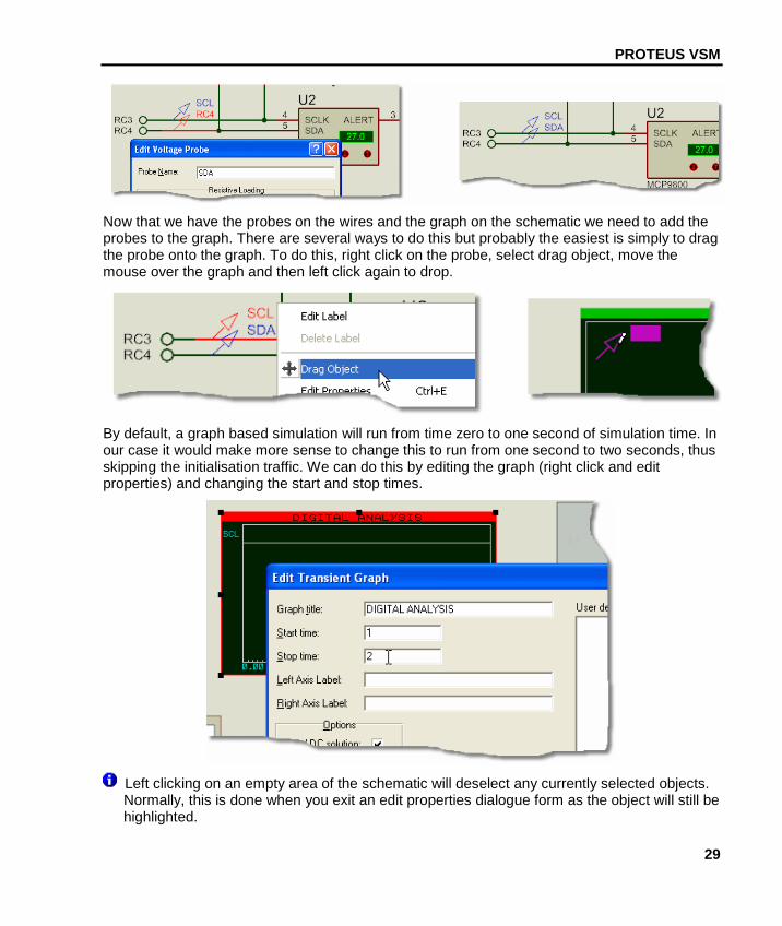
By default, the voltage probes will pick up the name of the terminal. It's useful to rename them to be more meaningful in the context of our simulation. You can do this by right clicking on the probe, editing its properties and then changing the name to the SCL and SDA respectively.

PROTEUS VSM

29

Now that we have the probes on the wires and the graph on the schematic we need to add the probes to the graph. There are several ways to do this but probably the easiest is simply to drag the probe onto the graph. To do this, right click on the probe, select drag object, move the mouse over the graph and then left click again to drop.

By default, a graph based simulation will run from time zero to one second of simulation time. In our case it would make more sense to change this to run from one second to two seconds, thus skipping the initialisation traffic. We can do this by editing the graph (right click and edit properties) and changing the start and stop times.

Left clicking on an empty area of the schematic will deselect any currently selected objects. Normally, this is done when you exit an edit properties dialogue form as the object will still be highlighted.


30

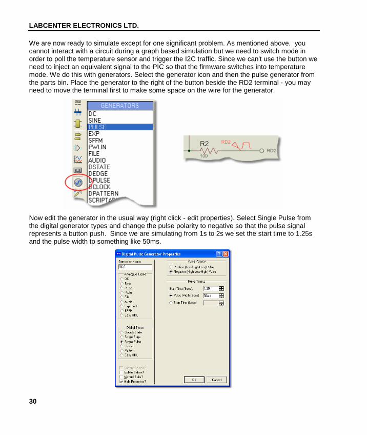
We are now ready to simulate except for one significant problem. As mentioned above, you cannot interact with a circuit during a graph based simulation but we need to switch mode in order to poll the temperature sensor and trigger the I2C traffic. Since we can't use the button we need to inject an equivalent signal to the PIC so that the firmware switches into temperature mode. We do this with generators. Select the generator icon and then the pulse generator from the parts bin. Place the generator to the right of the button beside the RD2 terminal - you may need to move the terminal first to make some space on the wire for the generator.

Now edit the generator in the usual way (right click - edit properties). Select Single Pulse from the digital generator types and change the pulse polarity to negative so that the pulse signal represents a button push. Since we are simulating from 1s to 2s we set the start time to 1.25s and the pulse width to something like 50ms.

PROTEUS VSM

31

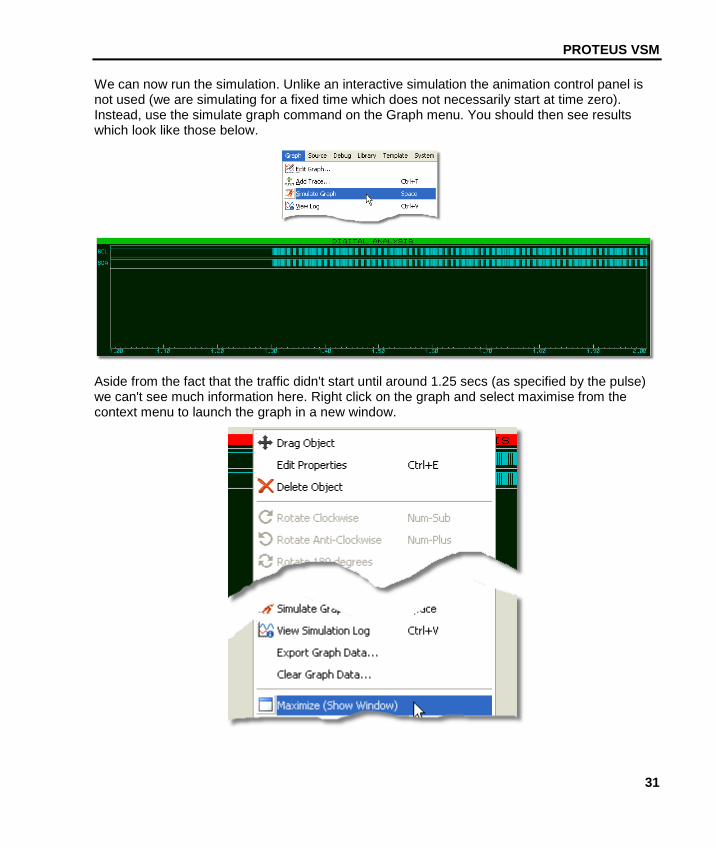
We can now run the simulation. Unlike an interactive simulation the animation control panel is not used (we are simulating for a fixed time which does not necessarily start at time zero). Instead, use the simulate graph command on the Graph menu. You should then see results which look like those below.

Aside from the fact that the traffic didn't start until around 1.25 secs (as specified by the pulse) we can't see much information here. Right click on the graph and select maximise from the context menu to launch the graph in a new window.


32

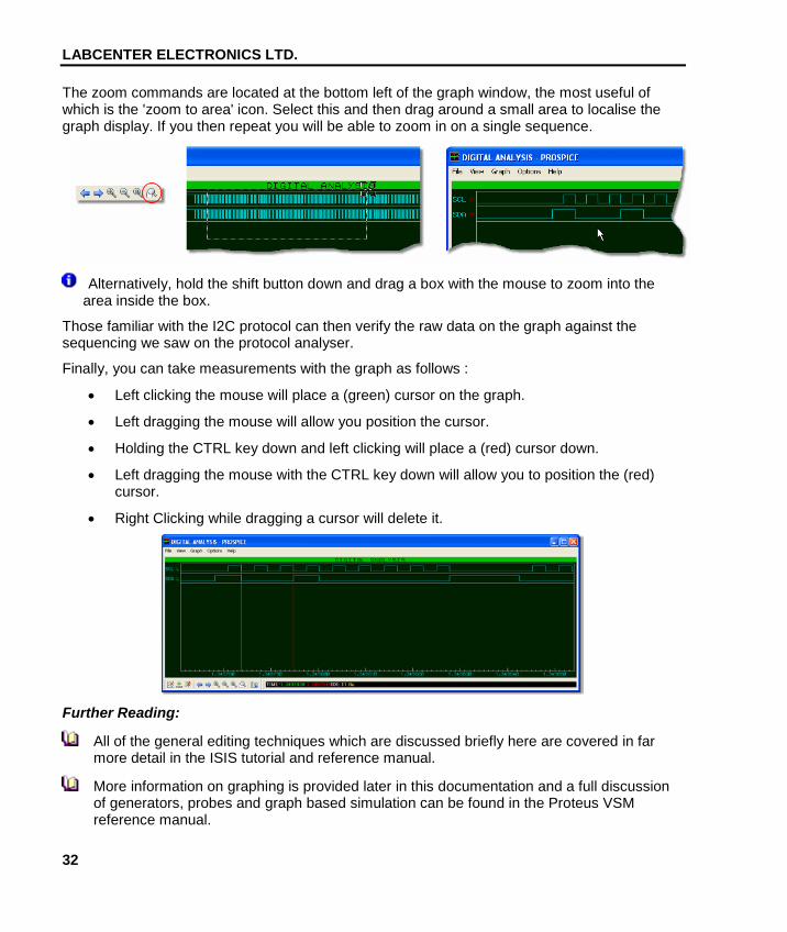
The zoom commands are located at the bottom left of the graph window, the most useful of which is the 'zoom to area' icon. Select this and then drag around a small area to localise the graph display. If you then repeat you will be able to zoom in on a single sequence.

Alternatively, hold the shift button down and drag a box with the mouse to zoom into the area inside the box.

Those familiar with the I2C protocol can then verify the raw data on the graph against the sequencing we saw on the protocol analyser.

Finally, you can take measurements with the graph as follows :

• Left clicking the mouse will place a (green) cursor on the graph.

• Left dragging the mouse will allow you position the cursor.

• Holding the CTRL key down and left clicking will place a (red) cursor down.

• Left dragging the mouse with the CTRL key down will allow you to position the (red) cursor.

• Right Clicking while dragging a cursor will delete it.

Further Reading:

All of the general editing techniques which are discussed briefly here are covered in far more detail in the ISIS tutorial and reference manual.

More information on graphing is provided later in this documentation and a full discussion of generators, probes and graph based simulation can be found in the Proteus VSM reference manual.

PROTEUS VSM

33

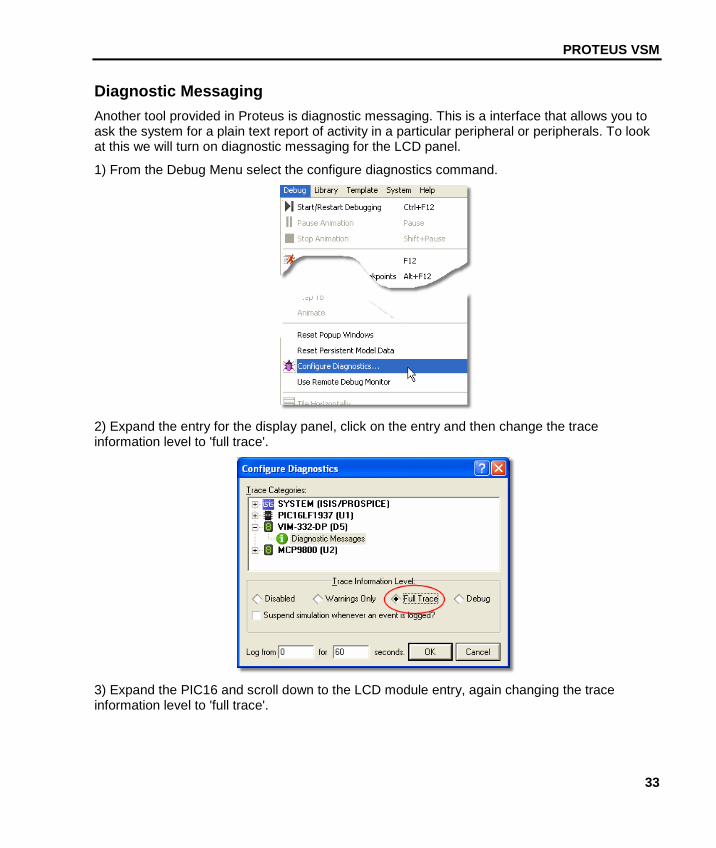
Diagnostic Messaging Another tool provided in Proteus is diagnostic messaging. This is a interface that allows you to ask the system for a plain text report of activity in a particular peripheral or peripherals. To look at this we will turn on diagnostic messaging for the LCD panel.

1) From the Debug Menu select the configure diagnostics command.

2) Expand the entry for the display panel, click on the entry and then change the trace information level to 'full trace'.

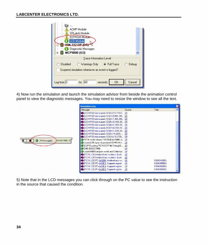
3) Expand the PIC16 and scroll down to the LCD module entry, again changing the trace information level to 'full trace'.


34

4) Now run the simulation and launch the simulation advisor from beside the animation control panel to view the diagnostic messages. You may need to resize the window to see all the text.

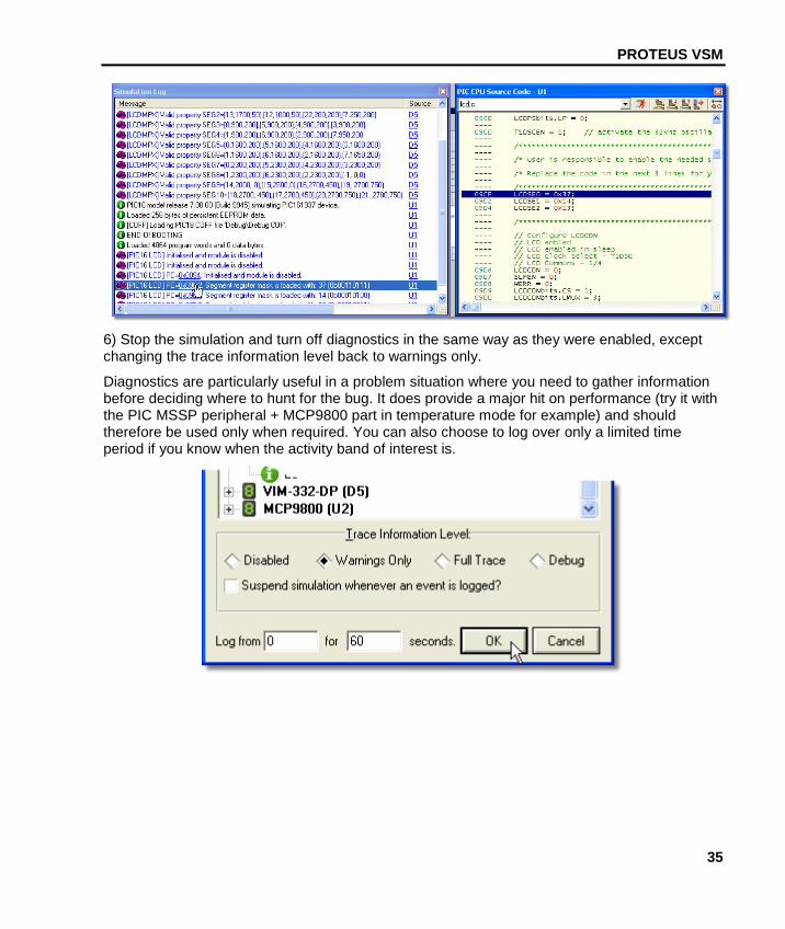
5) Note that in the LCD messages you can click through on the PC value to see the instruction in the source that caused the condition.

PROTEUS VSM

35

6) Stop the simulation and turn off diagnostics in the same way as they were enabled, except changing the trace information level back to warnings only.

Diagnostics are particularly useful in a problem situation where you need to gather information before deciding where to hunt for the bug. It does provide a major hit on performance (try it with the PIC MSSP peripheral + MCP9800 part in temperature mode for example) and should therefore be used only when required. You can also choose to log over only a limited time period if you know when the activity band of interest is.

36

GRAPH BASED TUTORIAL Introduction The purpose of this tutorial is to show you, by use of a simple amplifier circuit, how to perform a graph based simulation using PROTEUS VSM. It takes you, in a step-by-step fashion, through:

• Placing graphs, probes and generators.

• Performing the actual simulation.

• Using graphs to display results and take measurements.

• A survey of the some of the analysis types that are available.

The tutorial does not cover the use of ISIS in its general sense - that is, procedures for placing components, wiring them up, tagging objects, etc. This is covered to some extent in the Interactive Simulation Tutorial and in much greater detail within the ISIS manual itself. If you have not already made yourself familiar with the use of ISIS then you must do so before attempting this tutorial.

We do strongly urge you to work right the way through this tutorial before you attempt to do your own graph based simulations: gaining a grasp of the concepts will make it much easier to absorb the material in the reference chapters and will save much time and frustration in the long term.

Getting Started The circuit we are going to simulate is an audio amplifier based on a 741 op-amp, as shown overleaf. It shows the 741 in an unusual configuration, running from a single 5 volt supply. The feedback resistors, R3 and R4, set the gain of the stage to be about 10. The input bias components, R1, R2 and C1, set a false ground reference at the non-inverting input which is decoupled from the signal input.

As is normally the case, we shall perform a transient analysis on the circuit. This form of analysis is the most useful, giving a large amount of information about the circuit. Having completed the description of simulation with transient analysis, the other forms of analysis will be contrasted.

PROTEUS VSM

37

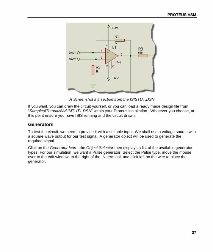
A Screenshot if a section from the ISISTUT.DSN

If you want, you can draw the circuit yourself, or you can load a ready made design file from "Samples\Tutorials\ASIMTUT1.DSN" within your Proteus installation. Whatever you choose, at this point ensure you have ISIS running and the circuit drawn.

Generators To test the circuit, we need to provide it with a suitable input. We shall use a voltage source with a square wave output for our test signal. A generator object will be used to generate the required signal.

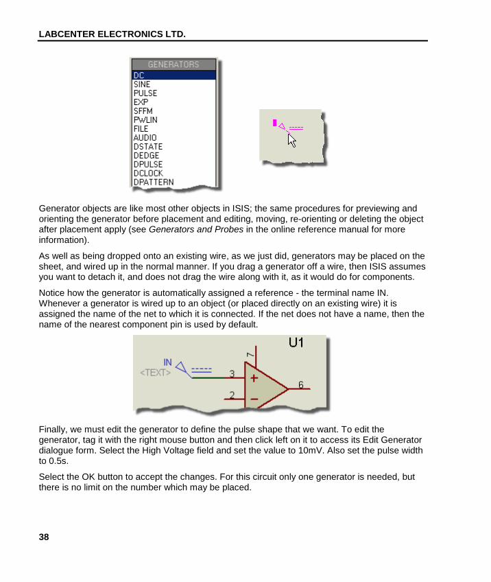
Click on the Generator Icon - the Object Selector then displays a list of the available generator types. For our simulation, we want a Pulse generator. Select the Pulse type, move the mouse over to the edit window, to the right of the IN terminal, and click left on the wire to place the generator.


38

Generator objects are like most other objects in ISIS; the same procedures for previewing and orienting the generator before placement and editing, moving, re-orienting or deleting the object after placement apply (see Generators and Probes in the online reference manual for more information).

As well as being dropped onto an existing wire, as we just did, generators may be placed on the sheet, and wired up in the normal manner. If you drag a generator off a wire, then ISIS assumes you want to detach it, and does not drag the wire along with it, as it would do for components.

Notice how the generator is automatically assigned a reference - the terminal name IN. Whenever a generator is wired up to an object (or placed directly on an existing wire) it is assigned the name of the net to which it is connected. If the net does not have a name, then the name of the nearest component pin is used by default.

Finally, we must edit the generator to define the pulse shape that we want. To edit the generator, tag it with the right mouse button and then click left on it to access its Edit Generator dialogue form. Select the High Voltage field and set the value to 10mV. Also set the pulse width to 0.5s.

Select the OK button to accept the changes. For this circuit only one generator is needed, but there is no limit on the number which may be placed.

PROTEUS VSM

39

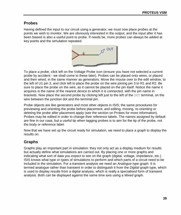
Probes Having defined the input to our circuit using a generator, we must now place probes at the points we wish to monitor. We are obviously interested in the output, and the input after it has been biased is also a useful point to probe. If needs be, more probes can always be added at key points and the simulation repeated.

To place a probe, click left on the Voltage Probe icon (ensure you have not selected a current probe by accident - we shall come to these later). Probes can be placed onto wires, or placed and then wired, in the same manner as generators. Move the mouse over to the edit window, to the left of U1 pin 3, and click left to place the probe on the wire joining pin 3 to R1 and R2. Be sure to place the probe on the wire, as it cannot be placed on the pin itself. Notice the name it acquires is the name of the nearest device to which it is connected, with the pin name in brackets. Now place the second probe by clicking left just to the left of the OUT terminal, on the wire between the junction dot and the terminal pin.

Probe objects are like generators and most other objects in ISIS; the same procedures for previewing and orienting the probe before placement, and editing, moving, re-orienting or deleting the probe after placement apply (see the section on Probes for more information). Probes may be edited in order to change their reference labels. The names assigned by default are fine in our case, but a useful tip when tagging probes is to aim for the tip of the probe, not the body or reference label.

Now that we have set up the circuit ready for simulation, we need to place a graph to display the results on.

Graphs Graphs play an important part in simulation: they not only act as a display medium for results but actually define what simulations are carried out. By placing one or more graphs and indicating what sort of data you expect to see on the graph (digital, voltage, impedance, etc.) ISIS knows what type or types of simulations to perform and which parts of a circuit need to be included in the simulation. For a transient analysis we need an Analogue type graph. It is termed analogue rather than transient in order to distinguish it from the Digital graph type, which is used to display results from a digital analysis, which is really a specialised form of transient analysis. Both can be displayed against the same time axis using a Mixed graph.


40

To place a graph, select the Graph icon: the Object Selector displays a list of the available graph types. Select the Analogue type, move the mouse over to the edit window, click the left mouse button once and then drag out a rectangle of the appropriate size, clicking the mouse button again to place the graph.

Graphs behave like most objects in ISIS, though they do have a few subtleties. We will cover the features pertinent to the tutorial as they occur, but the reference chapter on graphs is well worth a read. You can tag a graph in the usual way with the mouse button, and then (using the left mouse button) drag one of the handles, or the graph as a whole, about to resize and/or reposition the graph.

We now need to add our generator and probes on to the graph. Each generator has a probe associated with it, so there is no need to place probes directly on generators to see the input wave forms. There are three ways of adding probes and generators to graphs:

• The first method is to tag each probe/generator in turn and drag it over the graph and release it - exactly as if we were repositioning the object. ISIS detects that you are trying to place the probe/generator over the graph, restores the probe/generator to its original position, and adds a trace to the graph with the same reference as that of the probe/generator. Traces may be associated with the left or right axes in an analogue graph, and probes/generators will add to the axis nearest the side they were dropped. Regardless of where you drop the probe/generator, the new trace is always added at the bottom of any existing traces.

The second and third method of adding probes/generators to a graph both use the Add Trace command on the graph menu; this command always adds probes to the current graph (when there is more than one graph, the current graph is the one currently selected on the Graph menu).

• If the Add Trace command is invoked without any tagged probes or generators, then the Add Transient Trace dialogue form is displayed, and a probe can be selected from a list of all probes in the design (including probes on other sheets).

• If there are tagged probes/generators, invoking the Add Trace command causes you to be prompted to Quick Add the tagged probes to the current graph; selecting the No option invokes the Add Transient Trace dialogue form as previously described. Selecting the Yes option adds all tagged probes/generators to the current graph in alphabetical order.

We will Quick Add our probes and the generator to the graph. Either tag the probes and generators individually, or, more quickly, drag a tag box around the entire circuit - the Quick Add feature will ignore all tagged objects other than probes and generators. Select the Add Trace option from the Graph menu and answer Yes to the prompt. The traces will appear on the graph (because there is only one graph, and it was the last used, it is deemed to be the current graph). At the moment, the traces consist of a name (on the left of the axis), and an empty data area (the main body of the graph). If the traces do not appear on the graph, then it is probably too small for ISIS to draw them in. Resize the graph, by tagging it and dragging a corner, to make it sufficiently big.

PROTEUS VSM

41

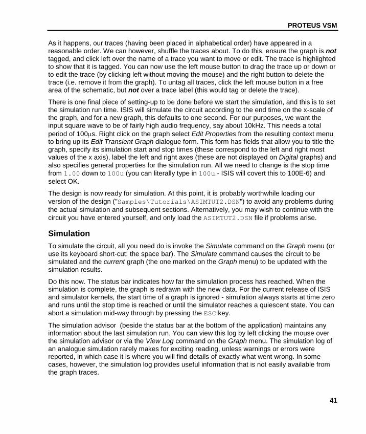
As it happens, our traces (having been placed in alphabetical order) have appeared in a reasonable order. We can however, shuffle the traces about. To do this, ensure the graph is not tagged, and click left over the name of a trace you want to move or edit. The trace is highlighted to show that it is tagged. You can now use the left mouse button to drag the trace up or down or to edit the trace (by clicking left without moving the mouse) and the right button to delete the trace (i.e. remove it from the graph). To untag all traces, click the left mouse button in a free area of the schematic, but not over a trace label (this would tag or delete the trace).

There is one final piece of setting-up to be done before we start the simulation, and this is to set the simulation run time. ISIS will simulate the circuit according to the end time on the x-scale of the graph, and for a new graph, this defaults to one second. For our purposes, we want the input square wave to be of fairly high audio frequency, say about 10kHz. This needs a total period of 100µs. Right click on the graph select Edit Properties from the resulting context menu to bring up its Edit Transient Graph dialogue form. This form has fields that allow you to title the graph, specify its simulation start and stop times (these correspond to the left and right most values of the x axis), label the left and right axes (these are not displayed on Digital graphs) and also specifies general properties for the simulation run. All we need to change is the stop time from 1.00 down to 100u (you can literally type in 100u - ISIS will covert this to 100E-6) and select OK.

The design is now ready for simulation. At this point, it is probably worthwhile loading our version of the design ("Samples\Tutorials\ASIMTUT2.DSN") to avoid any problems during the actual simulation and subsequent sections. Alternatively, you may wish to continue with the circuit you have entered yourself, and only load the ASIMTUT2.DSN file if problems arise.

Simulation To simulate the circuit, all you need do is invoke the Simulate command on the Graph menu (or use its keyboard short-cut: the space bar). The Simulate command causes the circuit to be simulated and the current graph (the one marked on the Graph menu) to be updated with the simulation results.

Do this now. The status bar indicates how far the simulation process has reached. When the simulation is complete, the graph is redrawn with the new data. For the current release of ISIS and simulator kernels, the start time of a graph is ignored - simulation always starts at time zero and runs until the stop time is reached or until the simulator reaches a quiescent state. You can abort a simulation mid-way through by pressing the ESC key.

The simulation advisor (beside the status bar at the bottom of the application) maintains any information about the last simulation run. You can view this log by left clicking the mouse over the simulation advisor or via the View Log command on the Graph menu. The simulation log of an analogue simulation rarely makes for exciting reading, unless warnings or errors were reported, in which case it is where you will find details of exactly what went wrong. In some cases, however, the simulation log provides useful information that is not easily available from the graph traces.


42

Launching the Simulation Advisor after a Simulation Run.

If you invoke the Simulate command a second time, you may notice something odd - no simulation occurs. This is because ISIS's partition management is clever enough to work out whether or not the part(s) of a design being probed by a particular graph have changed and thus it only performs a simulation when required. In terms of our simple circuit, nothing has changed, and therefore no simulation takes place. If for some reason you want to always re-simulate a graph, you can check the Always Simulate check box on the graphs Edit Transient Analysis dialogue form. If you are in doubt as to what was actually simulated, you can check the Log Netlist check box on the same dialogue form; this causes the simulator netlist to be included in the simulation log.

So the first simulation is complete. Looking at the traces on the graph, it’s hard to see any detail. To check that the circuit is working as expected, we need to take some measurements...

Taking Measurements A graph sitting on the schematic, alongside a circuit, is referred to as being minimised. To take timing measurements we must first maximise the graph. To do this, first ensure the graph is not tagged, and then click the left mouse button on the graph's title bar; the graph is redrawn in its own window. Along the top of the display, the menu bar is maintained. Below this, on the left side of the screen is an area in which the trace labels are displayed and to right of this are the traces themselves. At the bottom of the display, on the left is a toolbar, and to the right of this is a status area that displays cursor time/state information. As this is a new graph, and we have not yet taken any measurements, there are no cursors visible on the graph, and the status bar simply displays a title message.

The traces are colour coded, to match their respective labels. The OUT and U1(POS IP) traces are clustered at the top of the display, whilst the IN trace lies along the bottom. To see the traces in more detail, we need to separate the IN trace from the other two. This can be achieved by using the left mouse button to drag the trace label to the right-hand side of the screen. This causes the right y-axis to appear, which is scaled separately from the left. The IN trace now seems much larger, but this is because ISIS has chosen a finer scaling for the right axis than the left. To clarify the graph, it is perhaps best to remove the IN trace altogether, as the U1(POS IP) is just as useful. Click right on the IN label twice to delete it. The graph now reverts to a single, left hand side, y-axis.

We shall measure two quantities:

• The voltage gain of the circuit.

• The approximate fall time of the output.

These measurements are taken using the Cursors.

PROTEUS VSM

43

Each graph has two cursors, referred to as the Reference and Primary cursors. The reference cursor is displayed in red, and the primary in green. A cursor is always 'locked' to a trace, the trace a cursor is locked to being indicated by a small 'X' which 'rides' the waveform. A small mark on both the x- and y-axes will follow the position of the 'X' as it moves in order to facilitate accurate reading of the axes. If moved using the keyboard, a cursor will move to the next small division in the x-axis.

Let us start by placing the Reference cursor. The same keys/actions are used to access both the Reference and Primary cursors. Which is actually affected is selected by use of the CTRL key on the keyboard; the Reference cursor, as it is the least used of the two, is always accessed with the CTRL key (on the keyboard) pressed down. To place a cursor, all you need to do is point at the trace data (not the trace label - this is used for another purpose) you want to lock the cursor to, and click left. If the CTRL key is down, you will place (or move) the Reference cursor; if the CTRL key is not down, then you will place (or move) the Primary cursor. Whilst the mouse button (and the bkey for the Reference cursor) is held down, you can drag the cursor about. So, hold down (and keep down) the CTRL key, move the mouse pointer to the right hand side of the graph, above both traces, and press the left mouse button. The red Reference cursor appears. Drag the cursor (still with the CTRL key down) to about 70u or 80u on the x-axis. The title on the status bar is removed, and will now display the cursor time (in red, at the left) and the cursor voltage along with the name of the trace in question (at the right). It is the OUT trace that we want.

You can move a cursor in the X direction using the left and right cursor keys, and you can lock a cursor to the previous or next trace using the up and down cursor keys. The LEFT and RIGHT keys move the cursor to the left or right limits of the x-axis respectively. With the control key still down, try pressing the left and right arrow keys on the keyboard to move the Reference cursor along small divisions on the time axis.

Now place the Primary cursor on the OUT trace between 20u and 30u. The procedure is exactly the same as for the Reference cursor, above, except that you do not need to hold the CTRL key down. The time and the voltage (in green) for the primary cursor are now added to the status bar.

Also displayed are the differences in both time and voltage between the positions of the two cursors. The voltage difference should be a fraction above 100mV. The input pulse was 10mV high, so the amplifier has a voltage gain of 10. Note that the value is positive because the Primary cursor is above the Reference cursor - in delta read-outs the value is Primary minus Reference.

We can also measure the fall time using the relative time value by positioning the cursors either side of the falling edge of the output pulse. This may be done either by dragging with the mouse, or by using the cursor keys (don't forget the CTRL key for the Reference cursor). The Primary cursor should be just to the right of the curve, as it straightens out, and the Reference cursor should be at the corner at the start of the falling edge. You should find that the falling edge is a little under 10µs.


44

Using Current Probes Now that we have finished with our measurements, we can return to the circuit - just close the graph window in the usual way, or for speed you can press ESC on the keyboard. We shall now use a current probe to examine the current flow around the feedback path, by measuring the current into R4.

Current probes are used in a similar manner to voltage probes, but with one important difference. A current probe needs to have a direction associated with it. Current probes work by effectively breaking a wire, and inserting themselves in the gap, so they need to know which way round to go. This is done simply by the way they are placed. In the default orientation (leaning to the right) a current probe measures current flow in a horizontal wire from left to right. To measure current flow in a vertical wire, the probe needs to be rotated through 90° or 270°. Placing a probe at the wrong angle is an error, that will be reported when the simulation is executed. If in doubt, look at the arrow in the symbol. This points in the direction of current flow.

Select a current probe by clicking on the Current Probe icon. Click left on the clockwise Rotation icon such that the arrow points downwards. Then place the probe on the vertical wire between the right hand side of R4 and U1 pin 6. Add the probe to the right hand side of the graph by tagging and dragging onto the right hand side of the minimised graph. The right side is a good choice for current probes because they are normally on a scale several orders of magnitude different than the voltage probes, so a separate axis is needed to display them in detail. At the moment no trace is drawn for the current probe. Press the space bar to re-simulate the graph, and the trace appears.

Even from the minimised graph, we can see that the current in the feedback loop follows closely the wave form at the output, as you would expect for an op-amp. The current changes between 10µA and 0 at the high and low parts of the trace respectively. If you wish, the graph may be maximised to examine the trace more closely.

Frequency Analysis As well as transient analysis, there are several other analysis types available in analogue circuit simulation. They are all used in much the same way, with graphs, probes and generators, but they are all different variations on this theme. The next type of analysis that we shall consider is Frequency analysis. In frequency analysis, the x-axis becomes frequency (on a logarithmic scale), and both magnitude and phase of probed points may be displayed on the y-axes.

To perform a frequency analysis a Frequency graph is required. Click left on the Graph icon, to re-display the list of graph types in the object selector, and click on the Frequency graph type. Then place a graph on the schematic as before, dragging a box with the left mouse button. There is no need to remove the existing transient graph, but you may wish to do so in order to create some more space (click right twice to delete a graph).

PROTEUS VSM

45

Now to add the probes. We shall add both the voltage probes, OUT and U1(POS IP). In a frequency graph, the two y-axes (left and right) have special meanings. The left y-axis is used to display the magnitude of the probed signal, and the right y-axis the phase. In order to see both, we must add the probes to both sides of the graph. Tag and drag the OUT probe onto the left of the graph, then drag it onto the right. Each trace has a separate colour as normal, but they both have the same name. Now tag and drag the U1(POS IP) probe onto the left side of the graph only.

Magnitude and phase values must both be specified with respect to some reference quantity. In ISIS this is done by specifying a Reference Generator. A reference generator always has an output of 0dB (1 volt) at 0°. Any existing generator may be specified as the reference generator. All the other generators are in the circuit are ignored in a frequency analysis. To specify the IN generator as the reference in our circuit, simply tag and drag it onto the graph, as if you were adding it as a probe. ISIS assumes that, because it is a generator, you are adding it as the reference generator, and prints a message on status line confirming this. Make sure you have done this, or the simulation will not work correctly.

There is no need to edit the graph properties, as the frequency range chosen by default is fine for our purposes. However, if you do so (by pointing at the graph and pressing CTRL-E), you will see that the Edit Frequency Graph dialogue form is slightly different from the transient case. There is no need to label the axes, as their purpose is fixed, and there is a check box which enables the display of magnitude plots in dB or normal units. This option is best left set to dB, as the absolute values displayed otherwise will not be the actual values present in the circuit.

Now press the space bar (with the mouse over the frequency graph) to start the simulation. When it has finished, click left on the graph title bar to maximise it. Considering first the OUT magnitude trace, we can see the pass-band gain is just over 20dB (as expected), and the useable frequency range is about 50Hz to 20kHz. The cursors work in exactly the same manner as before - you may like to use the cursors to verify the above statement. The OUT phase trace shows the expected phase distortion at the extremes of the response, dropping to -90° just off the right of the graph, at the unity gain frequency. The high-pass filter effect of the input bias circuitry can be clearly seen if the U1(POS IP) magnitude trace is examined. Notice that the x-axis scale is logarithmic, and to read values from the axis it is best to use the cursors.

Swept Variable Analysis It is possible with ISIS to see how the circuit is affected by changing some of the circuit parameters. There are two analysis types that enable you to do this - the DC Sweep and the AC Sweep. A DC Sweep graph displays a series of operating point values against the swept variable, while an AC Sweep graph displays a series of single point frequency analysis values, in magnitude and phase form like the Frequency graph.

As these forms of analysis are similar, we shall consider just one - a DC Sweep. The input bias resistors, R1 and R2, are affected by the small current that flows into U1. To see how altering the value of both of these resistors affects the bias point, a DC Sweep is used.


46

To begin with place a DC Sweep graph on an unused space on the schematic. Then tag the U1(POS IP) probe and drag it onto the left of the graph. We need to set the sweep value, and this is done by editing the graph (point at it and press CTRL-E). The Edit DC Sweep Graph dialogue form includes fields to set the swept variable name, its start and ending values, and the number of steps taken in the sweep. We want to sweep the resistor values across a range of say 100kΩ to 5MΩ, so set the Start field to 100k and the Stop field to 5M. Click on OK to accept the changes.

Of course, the resistors R1 and R2 need to be altered to make them swept, rather than the fixed values they already are. To do this, click right and then left on R1 to edit it, and alter the Value field from 470k to X. Note that the swept variable in the graph dialogue form was left at X as well. Click on OK, and repeat the editing on R2 to set its value to X.

Now you can simulate the graph by pointing at it and pressing the space-bar. Then, by maximising the graph, you can see that the bias level reduces as the resistance of the bias chain increases. By 5MΩ it is significantly altered. Of course, altering these resistors will also have an effect on the frequency response. We could have done an AC Sweep analysis at say 50Hz in order to see the effect on low frequencies.

Noise Analysis The final form of analysis available is Noise analysis. In this form of analysis the simulator will consider the amount of thermal noise that each component will generate. All these noise contributions are then summed (having been squared) at each probed point in the circuit. The results are plotted against the noise bandwidth.

There are some important peculiarities to noise analysis:

• The simulation time is directly proportional to the number of voltage probes (and generators) in the circuit, since each one will be considered.

• Current probes have no meaning in noise analysis, and are ignored.

• A great deal of information is presented in the simulation log file.

• PROSPICE computes both input and output noise. To do the former, an input reference must be defined - this is done by dragging a generator onto the graph, as with a frequency reference. The input noise plot then shows the equivalent noise at the input for each output point probed.

To perform a noise analysis on our circuit, we must first restore R1 and R2 back to 470kΩ. Do this now. Then select a Noise graph type, and place a new graph on an unused area of the schematic. It is really only output noise we are interested in, so tag the OUT voltage probe and drag it onto the graph. As before, the default values for the simulation are fine for our needs, but you need to set the input reference to the input generator IN. The Edit Noise Graph dialogue form has the check box for displaying the results in dBs. If you use this option, then be aware that 0dB is considered to be 1 volt r.m.s. Click on Cancel to close the dialogue form.

PROTEUS VSM

47

Simulate the graph as before. When the graph is maximised, you can see that the values that result from this form of analysis are typically extremely small (pV in our case) as you might expect from a noise analysis of this type. But how do you track down sources of noise in your circuit? The answer lies in the simulation log. View the simulation log now, by pressing CTRL+V. Use the down arrow icon to move down past the operating point printout, and you should see a line of text that starts

Total Noise Contributions at...

This lists the individual noise contributions (across the entire frequency range) of each circuit element that produces noise. Most of the elements are in fact inside the op-amp, and are prefixed with U1_. If you select the Log Spectral Contributions option on the Edit Noise Graph dialogue form, then you will get even more log data, showing the contribution of each component at each spot frequency.


48

vsm tutorial

Documents

Transcript of vsm tutorial