Traitement des Images etVision Artificielle

Segmentation

Martin de La Gorce

martin.de-la-gorce@enpc.fr

February 2015

1 / 1

Segmentation

The goal of segmentation is to group together similar-lookingpixels i.e. to partition the image into uniform regions

The problem of segmentation is often not well defined : whatconsists in a good segmentation is often subjective anddepends on the application

2 / 1

What is segmentation used for ?

Segmentation can be use

for itself, for example to quantify the size of an organ in aMRI image

As as preliminary step is an higher level task such asobject recognition or scene understanding

3 / 1

Limit of Edges

The problem with edge is that:they do not necessarly define the boundaries of the objectwe want to segment .Some object boundaries can present almost no edgesedges do not always define closed non intersecting curvesand thus we cannot define regions

edges matchesboundaries

edges are missingat boundaries and weget extra "clutter"

4 / 1

Edges

two approaches

find closed curves that contain strong edges

find regions that contain statistical distribution of pixelintensities that are uniform across each region

obviously these two approaches are not exclusive and can becombined

5 / 1

Region based segmentation

0 50 100 150 200 2500100020003000400050006000700080009000

image histogramme seuils=45,120

How can we determine automatically were to put thethreshold ?

How can we deal with color images ?

How can we remove isolated pixels in the segmentation ?

6 / 1

Color normalization

Let I(i , j , c) denote the intensity of the image at pixel (i , j)in thecth color chanelIn order to cope change of lighting condition across an object,We consider the intensity normalized image defined by:

I(i , j , c) = I(i , j , c)/L(i , j)

with L the luminance defined by

L(i , j) =√

I(i , j , 0)2 + I(i , j , 1)2 + I(i , j , 2)2

I I7 / 1

Color normalization

I I

8 / 1

Color space Clustering

We cluster the colors into compact groups in the color space,using for example k-means (see next slides)

nomalized colors distribution clusters

9 / 1

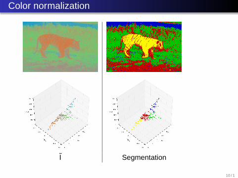
Color normalization

I Segmentation

10 / 1

K-means

Goal: Given N points p1, . . . , pN we try to find k clusters centersc1, , ck and N labels l1, . . . , lN with li ∈ {1, . . . , k} that minimizeE with

E =n∑

i=1

‖cli − pi‖2

11 / 1

K-means

E =n∑

i=1

‖cli − pi‖2

We denote sj the set of point with label j i.e

sj = {i |li = j} ⊂ {p1, . . . , pN}

We get an alternative formulation of E :

E =k∑

j=1

∑

i∈sj

‖cj − pi‖2

12 / 1

K-means

E =n∑

i=1

‖cli − pi‖2

We minimize E iteratively by minimizing E alternatively withrespect the (c1, . . . , ck ) and with respect to (l1, . . . , lN):

The minimization of E with respect to each center cj isdone by taking the barycenter of each cluster:

cj =1|sj |

∑

i∈sj

pi

with |sj | the number of point in sj

The minimization of E with respect to the labels is done bychoosing for each point the label corresponding to thenearest center:

li = argminj(‖cj − pi‖2)

13 / 1

K-means

Updating labels: Each data point find wich center it is theclosest to. We can visualize this using the voronoi regionsassociate to the centers:

14 / 1

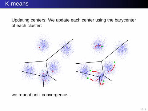
K-means

Updating centers: We update each center using the barycenterof each cluster:

we repeat until convergence...

15 / 1

K-means

We initialize the algorithm with random centers chosenamong the points

We iterate until convergence. The convergence isguarantied in a finite number of iteration by the fact that wereduce E at each step and the set of possible labels isfinite.

Limitations:

The solution we find at convergence can be a localminimum: starting with a different set of center can lead toan different solution at convergence.

We have to choose the manually the number of centers k

16 / 1

Using pixel neighboring

A segmentation of an image base on pixels clusteringtakes a per-pixel decisions an lead with segmentationregion with many isolated points

We can remove isolated points by replacing the label ofeach pixel using the label that is the most represented in asmall neighborhood (majority filter)

We actually want to change only the label of pixels whose coloris far from their respective center...

17 / 1

Using pixel neighboring

A better approach consists in minimizing a function that tradesbetween

the distance of the color of each to the cluster center

the difference of between labels of neighboring pixels:

This can be formalized as the minimization of a function E :

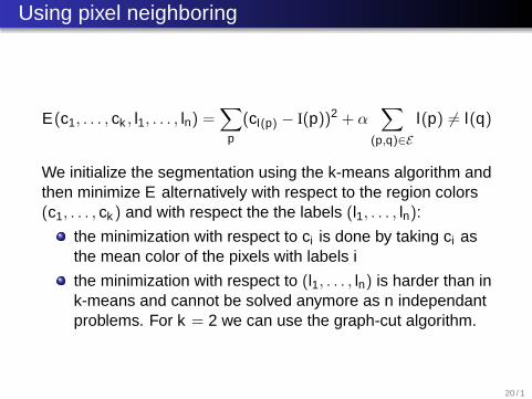
E(c1, . . . , ck , l1, . . . , ln) =∑

p

(cl(p)− I(p))2 +α∑

(p,q)∈E

[l(p) 6= l(q)]

with [a 6= b] = 1 id a 6= b and [a 6= b] = 0 is a = b and E the setof edges between neighboring pixels

18 / 1

Using pixel neighboring

E(c1, . . . , ck , l1, . . . , ln) =∑

p

(cl(p) − I(p))2 + α∑

(p,q)∈E

l(p) 6= l(q)

This model is know as the Pott model and the finding aglobal minimum is NP-Hard.

The equivalent continuous formulation is refered in theliterature as the piecewise constant Mumford-Shahfunctional.

19 / 1

Using pixel neighboring

E(c1, . . . , ck , l1, . . . , ln) =∑

p

(cl(p) − I(p))2 + α∑

(p,q)∈E

l(p) 6= l(q)

We initialize the segmentation using the k-means algorithm andthen minimize E alternatively with respect to the region colors(c1, . . . , ck ) and with respect the the labels (l1, . . . , ln):

the minimization with respect to ci is done by taking ci asthe mean color of the pixels with labels i

the minimization with respect to (l1, . . . , ln) is harder than ink-means and cannot be solved anymore as n independantproblems. For k = 2 we can use the graph-cut algorithm.

20 / 1

Graph-cut algorithm

We consider a graph with nodes V = {v1, . . . , Vn} andoriented edges {e1, . . . , ek} ⊂ V × V with associatednon-negative weights w1, . . . , wk

Given a source node s ∈ V and a target node t ∈ V , wedefine a s-t cut as a binary partition of (S, T ) of V(S⋃

T = V ,S⋂

T = ∅) such that s ∈ S and t ∈ T

21 / 1

Graph-cut algorithm

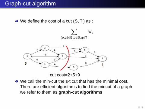
We define the cost of a cut (S, T ) as :

∑

(p,q)∈E ,p∈S,q∈T

we

cut cost=2+5+9

We call the min-cut the s-t cut that has the minimal cost.There are efficient algorithms to find the mincut of a graphwe refer to them as graph-cut algorithms

22 / 1

min-cut / max-flow

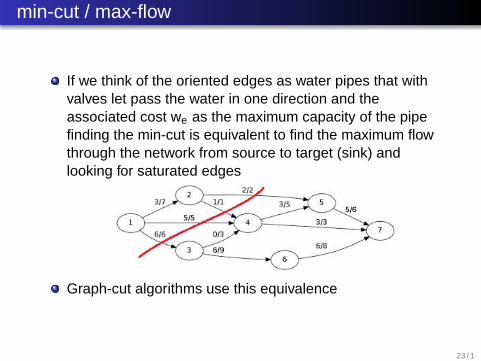
If we think of the oriented edges as water pipes that withvalves let pass the water in one direction and theassociated cost we as the maximum capacity of the pipefinding the min-cut is equivalent to find the maximum flowthrough the network from source to target (sink) andlooking for saturated edges

Graph-cut algorithms use this equivalence

23 / 1

Graph-cut algorithm

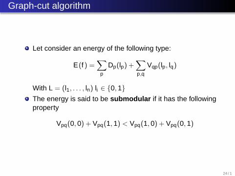
Let consider an energy of the following type:

E(f ) =∑

p

Dp(lp) +∑

p,q

Vqp(lp, lq)

With L = (l1, . . . , ln) li ∈ {0, 1}

The energy is said to be submodular if it has the followingproperty

Vpq(0, 0) + Vpq(1, 1) < Vpq(1, 0) + Vpq(0, 1)

24 / 1

Graph-cut algorithm

Let consider a an energy,

E(f ) =∑

p

Dp(lp) +∑

p,q

Vqp(lp, lq)

If E is submodular, then we can create a graph G(V , E)such that the global of E is obtained by solving the min-cutproblem G using lp = 0 ⇔ p ∈ T , lp = 1 ⇔ p ∈ S.When Vpq(0, 0) = Vpq(1, 1) = 0 the construction of thegraph is easy:

25 / 1

Graph-cut algorithm

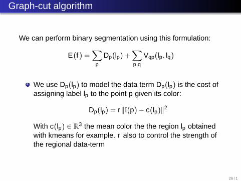
We can perform binary segmentation using this formulation:

E(f ) =∑

p

Dp(lp) +∑

p,q

Vqp(lp, lq)

We use Dp(lp) to model the data term Dp(lp) is the cost ofassigning label lp to the point p given its color:

Dp(lp) = r‖I(p) − c(lp)‖2

With c(lp) ∈ R3 the mean color the the region lp obtainedwith kmeans for example. r also to control the strength ofthe regional data-term

26 / 1

Graph-cut algorithm

E(f ) =∑

p

Dp(lp) +∑

p,q

Vqp(lp, lq)

We use Vqp(lp, lq) to model a prior that neighboring pixelshave in general the same label using

Vqp(0, 0) = Vqp(1, 1) = 0

Vqp(0, 1) = Vqp(1, 0) = α

With α a factor that control the smoothing of thesegmentation

Using this definition of Vpq, then sum∑

p,q Vqp(lp, lq)measures the length of the boundary between the tworegions

27 / 1

Graph-cut algorithm

α = 0.01 α = 0.05

α = 0.1 α = 0.3

28 / 1

Graph-cut algorithm

E(f ) =∑

p

Dp(lp) +∑

p,q

Vqp(lp, lq)

We can use Dp(0) = ∞ to constrain some points to havelabel 1 and Dp(1) = ∞ to constrain other points to havelabel 0. This allow a user to specify by hand some pointsthat have to be the object or the background

29 / 1

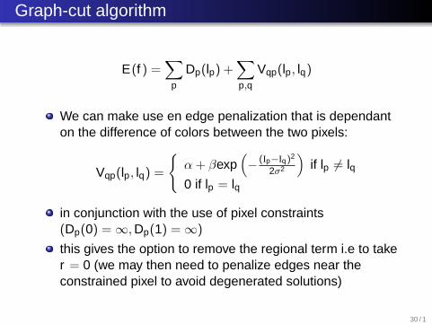
Graph-cut algorithm

E(f ) =∑

p

Dp(lp) +∑

p,q

Vqp(lp, lq)

We can make use en edge penalization that is dependanton the difference of colors between the two pixels:

Vqp(lp, lq) =

{α + βexp

(− (Ip−Iq)2

2σ2

)if lp 6= lq

0 if lp = lq

in conjunction with the use of pixel constraints(Dp(0) = ∞, Dp(1) = ∞)

this gives the option to remove the regional term i.e to taker = 0 (we may then need to penalize edges near theconstrained pixel to avoid degenerated solutions)

30 / 1

Graph-cut algorithm

31 / 1

Multi-label segmentation

Coming back the the original multi-label formulation;

E(c1, . . . , ck , l1, . . . , ln) =∑

p

(cl(p) − I(p))2 +∑

(p,q)∈E

l(p) 6= l(q)

the minimization with respect the the labels (l1, . . . , ln) whenk > 2 can be done using extensions of the graph cut algorithmssuch as the αβ − swap algorithm as other random-markov fieldinference methods.

32 / 1

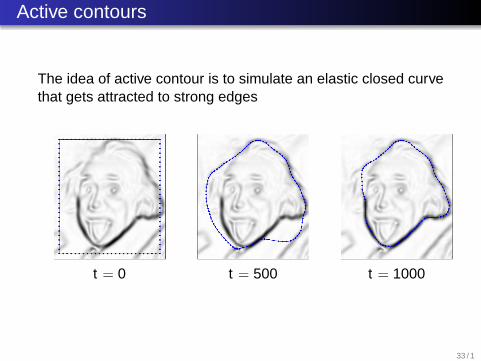
Active contours

The idea of active contour is to simulate an elastic closed curvethat gets attracted to strong edges

t = 0 t = 500 t = 1000

33 / 1

Active contours

We look for a smooth closed curve that contain strong edgeswe parameterize the curve using a function c that goesfrom [0, 1] into R2: t → c(t) = (x(t), y(t)). We havec(0) = c(1)We define an image H that has low value for point wherethe gradient of the image is large for example

H(x , y) = −‖∇I(x , y)‖

The amount of strong edges contained by the curve ismeasured using a data term

∫ 1

t=0H(c(t))dt =

∫ 1

t=0H(x(t), y(t))

34 / 1

Active contours

The smoothness of the curve is evaluated using tworegularization terms :

the first term is the integral of the squared speed of thecurve (interpreting t as the time):

∫ 1

t=0

∥∥∥∥

dcdt

∥∥∥∥

2

(t)dt =

∫ 1

t=0x ′(t)2 + y ′(t)2dt

its minimization makes the curve contract like an elasticmembrane

the second term is the integral of the squared accelerationof the curve:

∫ 1

t=0

∥∥∥∥

d2cd2t

∥∥∥∥

2

(t)dt =

∫ 1

t=0(x ′′(t)2 + y ′′(t)2)

its minimization makes the curve behave like a thin-plate

35 / 1

Active contours

We look for a smooth closed curve that contain strong edges byminimizing a weighted sum of the three terms

E(c) =

∫ 1

t=0H(c(t))dt + α

∫

t

∥∥∥∥

dcdt

∥∥∥∥

2

(t)dt + β

∫

t

∥∥∥∥

d2cd2t

∥∥∥∥

2

(t)dt

36 / 1

Active contours

The curve remains at the point with the the strongestgradient is the global minimum: not very interesting

Local minimums are more interesting. The local minima ofthe snake energy comprise the set of alternative solutions

We need to find several local minimas and use an higherlevel reasoning that allows to chose among them.

Or using supervision we perform a local search startingfrom a position not too far from the boundary of the object

37 / 1

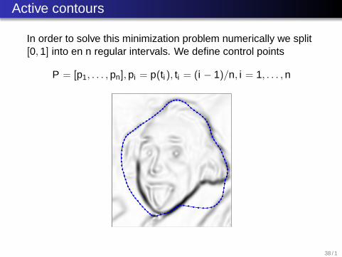
Active contours

In order to solve this minimization problem numerically we split[0, 1] into en n regular intervals. We define control points

P = [p1, . . . , pn], pi = p(ti), ti = (i − 1)/n, i = 1, . . . , n

38 / 1

Active contours

Using h = 1/n we can approximate the first and second orderderivative of c as follows:

dcdt

(ti) 'pi+1 − pi

hd2cd2t

(ti) 'pi−1 − 2pi + pi+1

h2

with pn+1 = p1 et p−1 = pn

39 / 1

Active contours

We approximate the integrals by finite sums

E(P) = Edata(P) + Eelastic(P) + Ethinplate(P)

With:

Edata(P) = h∑

i

C(pi)

Eelastic(P) =αhh2

n∑

i=1

‖pi − pi+1‖2

Ethinplate(P) =βhh4

n∑

i=1

‖pi−1 + pi+1 − 2pi‖2

with h = 1/n, pn+1 = p1 et p−1 = pn

40 / 1

Active contours

We will perform a gradient descent.

The gradient decompose into the sum of three gradients

∂Edata

∂pi= h∇H(pi)

∂Eelastic

∂pi=

2α

h(−pi−1 + 2pi − pi+1)

∂Ethinplate

∂pi=

2β

h3 (pi−2 − 4pi−1+6pi − 4pi+1 + pi+1)

If the function f is interpreted as an energy , the oppositeof each gradient can be interpreter as a "force":

the data term creates forces that pull the model toward highgradient regionthe elastic term create forces that contract the curvethe thin-plate term create forces that smoothes the curve

41 / 1

Active contours

We will rewrite the previous equations in a matrix from.We introduce the sparse circulant matrix D :

D =

−1 1 0 ∙ ∙ ∙ 0

0. . .

. . .. . .

......

. . .. . .

. . . 00 ∙ ∙ ∙ 0 −1 11 0 ∙ ∙ ∙ 0 −1

Using the froebenius norm on matrices ‖X‖ =∑

ij X 2ij ,we have

Eelastic(P) =α

h‖DP‖2

Ethinplate(P) =β

h3 ‖DT DP‖2

42 / 1

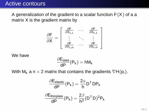
Active contours

A generalization of the gradient to a scalar function F (X ) of a amatrix X is the gradient matrix by

∂F∂X

=

∂F∂X1,1

∙ ∙ ∙ ∂F∂Xn,1

.... . .

...∂F

∂X1,m∙ ∙ ∙ ∂F

∂Xn,m

We have∂Edata

dP(Pk ) = hMk

With Mk a n × 2 matrix that contains the gradients ∇H(pi).

∂Eelastic

dP(Pk ) =

2α

hDT DPk

∂Ethinplate

dP(Pk ) =

2β

h3 (DT D)2Pk

43 / 1

Active contours

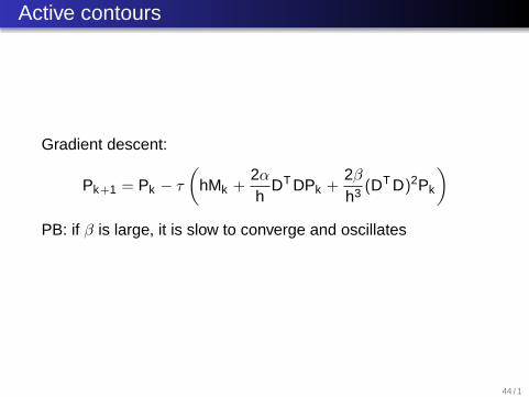
Gradient descent:

Pk+1 = Pk − τ

(

hMk +2α

hDT DPk +

2β

h3 (DT D)2Pk

)

PB: if β is large, it is slow to converge and oscillates

44 / 1

Majoration-Minimization

Reminder from last class:Instead of minimizing directly E(P), the Majoration-Minimizationapproach consists in solving a sequence of easier minimizationproblems Pk+1 = argminxGk (P)

The MM method requires that

Each function Gk (P) is majoring E i.e. ∀x : Gk (P) ≥ E(P)

Gk and E touch each other at Pk i.e Gk (Pk ) = E(Pk )

One dimensional illustration:

45 / 1

Active contours

For λ big enough (larger that the largest curvature of H) wehave for any p0:

∀p ∈ R2 : H(p) ≤ H(p0) + ∇H(p0) × (p − p0) + λ‖p − p0|2

x

H(x)

x

H(x)

λ too small λ big enough

We have a majoration of H that touches H en p0

46 / 1

Active contours: Majoration-Minimization

We iterate with Pk = argminPGk (P) with

Gk (P) = hn∑

i=1

(H(pi,k−1) + ∇H(pi,k−1) × (pi − pi,k−1)

)

+ λh‖P − Pk−1‖2 +

α

h‖DP‖2 +

β

h3 ‖DT DP‖2

(1)

Gk (P) is a majoration of E(P) such that E(Pk ) = GK (Pk ) andwe have a valid majoration -minimization scheme

47 / 1

Active contours: Majoration-Minimization

Pk = argminPGk (P)

We rewrite

n∑

i=1

∇H(pi,k−1) × (pi − pi,k−1) =< M(Pk−1), (P − Pk−1) >

With Mk−1 the n × 2 matrix that contains the 2D gradientsMk−1[i , :] = ∇H(pi,k−1).The gradient matrix of Gk writes

∂Gk

∂P(P)T = hMk−1 + 2λh(P − Pk−1) +

2α

hDT DP +

2β

h3 (DT D)2P

48 / 1

Active contours: Majoration-Minimization

∂Gk

∂P(P)T = hMk−1 + 2λh(P − Pk−1) +

2α

hDT DP +

2β

h3 (DT D)2P

We rewrite it as :

∂Gk

∂P(P)T = 2h

(12

Mk−1 − λPk−1 + AP)

with

A = λId +α

h2 DT D +β

h4 (DT D)2

49 / 1

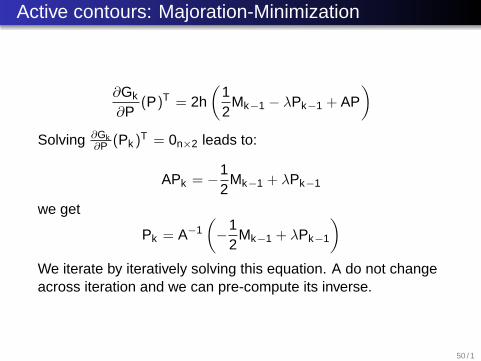
Active contours: Majoration-Minimization

∂Gk

∂P(P)T = 2h

(12

Mk−1 − λPk−1 + AP)

Solving ∂Gk∂P (Pk )T = 0n×2 leads to:

APk = −12

Mk−1 + λPk−1

we get

Pk = A−1(

−12

Mk−1 + λPk−1

)

We iterate by iteratively solving this equation. A do not changeacross iteration and we can pre-compute its inverse.

50 / 1

Active contours: Majoration-Minimization

t = 0 t = 200 t = 400

t = 600 t = 800 t = 1000 51 / 1