The Mechanisms of Alcohol Control - UCSC Directory of ...cdobkin/Papers/2016 The Mechanisms...
86
The Mechanisms of Alcohol Control By CHRISTOPHER S. CARPENTER, CARLOS DOBKIN, and CASEY WARMAN A substantial economics literature documents that tighter alcohol controls reduce alcohol- related harms, but far less is known about mechanisms. We use the universe of Canadian mortality records to document that Canada’s Minimum Legal Drinking Age (MLDA) significantly reduces mortality rates of young men but has much smaller effects on women. Using drinking data that are far more detailed than in prior work, we document that the MLDA substantially reduces ‘extreme’ drinking among men but not women. Our results suggest that alcohol control efforts targeting young adults should focus on reducing extreme drinking behavior. Christopher S. Carpenter is a Professor in the Department of Economics at Vanderbilt University. Carlos Dobkin is a Professor in the Department of Economics at the University of California Santa Cruz. Casey Warman is an Assistant Professor in the Department of Economics at Dalhousie University. The authors thank three anonymous referees, Phil DeCicca, Michael Haan, Beau Kilmer, Emma Pierard, Courtney Ward and numerous seminar and conference participants for very valuable comments. The authors also thank Heather Hobson for assistance at the Atlantic Research Data Centre at Dalhousie University. The research in this paper uses confidential versions of the Canadian Community Health Surveys, the National Population Health Surveys, and Canadian vital statistics data. Carpenter and Dobkin gratefully acknowledge an award from NIH/NIAAA #RO1 AA017302-01. While the research and analysis are based on data from Statistics Canada, the opinions expressed do not represent the views of Statistics Canada. The usual caveats apply. The data used in this article are restricted by Statistics Canada. Readers interested in obtaining the data can contact Christopher S. Carpenter, 2301 Vanderbilt Place, Department of Economics, Vanderbilt University, Nashville, TN, 37235. Email: [email protected].
-
Upload
vuongkhanh -
Category
Documents
-
view
212 -
download
0
Transcript of The Mechanisms of Alcohol Control - UCSC Directory of ...cdobkin/Papers/2016 The Mechanisms...
The Mechanisms of Alcohol Control
By CHRISTOPHER S. CARPENTER, CARLOS DOBKIN, and CASEY WARMAN
A substantial economics literature documents that tighter alcohol controls reduce alcohol-
related harms, but far less is known about mechanisms. We use the universe of Canadian
mortality records to document that Canada’s Minimum Legal Drinking Age (MLDA)
significantly reduces mortality rates of young men but has much smaller effects on women. Using
drinking data that are far more detailed than in prior work, we document that the MLDA
substantially reduces ‘extreme’ drinking among men but not women. Our results suggest that
alcohol control efforts targeting young adults should focus on reducing extreme drinking
behavior.
Christopher S. Carpenter is a Professor in the Department of Economics at Vanderbilt
University. Carlos Dobkin is a Professor in the Department of Economics at the University of
California Santa Cruz. Casey Warman is an Assistant Professor in the Department of Economics
at Dalhousie University. The authors thank three anonymous referees, Phil DeCicca, Michael
Haan, Beau Kilmer, Emma Pierard, Courtney Ward and numerous seminar and conference
participants for very valuable comments. The authors also thank Heather Hobson for assistance
at the Atlantic Research Data Centre at Dalhousie University. The research in this paper uses
confidential versions of the Canadian Community Health Surveys, the National Population
Health Surveys, and Canadian vital statistics data. Carpenter and Dobkin gratefully
acknowledge an award from NIH/NIAAA #RO1 AA017302-01. While the research and analysis
are based on data from Statistics Canada, the opinions expressed do not represent the views of
Statistics Canada. The usual caveats apply. The data used in this article are restricted by
Statistics Canada. Readers interested in obtaining the data can contact Christopher S. Carpenter,
2301 Vanderbilt Place, Department of Economics, Vanderbilt University, Nashville, TN, 37235.
Email: [email protected].

Carpenter, Dobkin, and Warman 1
I. Introduction
A substantial literature in economics documents that restricting access to alcohol reduces
alcohol-related harms such as mortality, crime, and risky sexual behavior.1 Motor vehicle
fatalities have received the most attention from economists due to the availability of high quality
outcome data and the fact they are the leading cause of death for young adults age 15-20 in the
United States.2 Researchers have studied how motor vehicle fatalities respond to alcohol control
policies such as: alcohol excise taxes (Cook 1981; Dee 1999; and others); drunk driving laws
(Eisenberg 2003; Grant 2010; and others); restrictions on the days and hours of alcohol sales
(Stehr 2010; Lovenheim and Steefel 2009; Biderman et al. 2010; and others); and minimum legal
drinking ages (MLDAs) (Cook and Tauchen 1984; Dee 1999; Lovenheim and Slemrod 2009;
Carpenter and Dobkin 2009; 2011; and others). Many of these studies have focused specifically
on youth fatalities, in part because multiple alcohol control policies are explicitly youth-targeted
(e.g., Zero Tolerance drunk driving laws and MLDAs) (see Bonnie and O’Connell 2004 for a
review).
However, there is limited evidence on how these laws affect the frequency and intensity
of alcohol consumption and which of the changes in alcohol consumption result in the reduction
in alcohol-related harms. Compared to the hundreds of studies on the effects of stricter alcohol
control policies on fatalities and other acute outcomes described in a recent review of the
literature by Wagenaar and Toomey (2002), only a few studies document their effects on
drinking (for examples see Kenkel 1995 and Sloan et al. 1995). Moreover, only a handful of
these use quasi-experimental designs (for examples see Dee 1999; Carpenter 2004; and Crost
and Rees 2013), and we are not aware of any that credibly adjudicate among the multiple
possible mechanisms through which alcohol control policies can reduce alcohol-related harms.3

Carpenter, Dobkin, and Warman 2
We fill this gap in the literature by combining a quasi-experimental approach (described
below) with extremely detailed Canadian data on daily alcohol consumption that allows us to
measure the entire distribution of drinking behavior. Our data are far superior to those used in
most previous work on this topic and which generally ask survey respondents only about past
year or past month drinking participation and heavy episodic or ‘binge’ drinking (typically
defined by public health scholars as five or more drinks consumed at one sitting for a man and
four or more drinks for a woman). These measures are problematic for several reasons,
including the fact that the threshold for defining binge drinking is arbitrary.4 In addition the
evidence uniquely linking binge drinking (as opposed to lighter or heavier drinking) to adverse
events is sparse. This is due to the fact that without very rich measures of alcohol consumption
and variation in how laws restricting access to alcohol affect drinking intensity it is not possible
to identify what levels of drinking are causing adverse outcomes.
We know from alcohol pharmacology that alcohol has very different effects depending
on how much is consumed.5 For example, 1 or 2 drinks consumed in one sitting for an average
180 pound man leads to a blood alcohol concentration (BAC) of less than 0.05 and is
characterized by increased sociability and euphoria with relatively little impairment. At 4 or 5
drinks (the standard definition of binge drinking) that same person will have a BAC of around
0.06 to 0.10 and is likely to suffer from impairments in judgment, coordination, depth
perception, and peripheral vision. But 8 or 10 drinks consumed in one sitting results in much
more severe deficits, including substantial compromises in reaction time and motor skills. Thus,
we know that different intensities of alcohol consumption lead to different physiologic
responses, highlighting the importance of understanding the effects of alcohol controls on the full
distribution of drinking intensity.

Carpenter, Dobkin, and Warman 3
Understanding what dimensions of alcohol consumption are responsible for the
substantial effects of tighter alcohol control on alcohol-related harms is also important because
studies examining the effect of stricter alcohol control on drinking behaviors demonstrate that
alcohol consumption can be very responsive to public policy. Thus, if we knew what types of
alcohol consumption were responsible for most of the alcohol-related harms, it is possible that
we could develop interventions tailored to affect these particular margins.6
Our approach to documenting the mechanisms of alcohol control is to use variation in
alcohol access induced by the Minimum Legal Drinking Age in Canada.7 Following prior work
for the United States (Carpenter and Dobkin 2009), we use a regression discontinuity approach
and examine the age profile of deaths in Canada around the MLDA.8 Using confidential
microdata on the universe of deaths in Canada from 1980 to 2008 with information on exact date
of birth and date of death of each decedent, we first confirm the basic result found in prior US
work: namely, that Canada’s MLDA significantly affects mortality. We estimate that total
deaths increase significantly by about 6 percent at the MLDA, and this is almost entirely
attributable to a 17 percent increase in motor vehicle accident mortality. Moreover, we find a
stark gender difference: the MLDA has large and significant effects at reducing deaths among
young men but has much smaller and statistically insignificant effects on deaths among young
women.
We then turn to unusually detailed survey data on alcohol consumption from Canadian
health surveys. In these surveys respondents are asked how many drinks they consumed on each
of the seven days prior to the interview date. As noted above, this information allows us to
document, for the first time in the literature, the full distribution of drinking frequency and
intensity among young adults. It also allows us to determine exactly how the frequency and
Carpenter, Dobkin, and Warman 4
intensity of alcohol consumption change when people are allowed to drink legally. Similar
analyses are not possible with most surveys in the United States which typically only ask about
two thresholds: any drinking and binge drinking. This limitation of existing US data turns out to
be very important. Specifically, we document the first evidence that ‘extreme’ drinking – which
we define as consuming 8 (10) or more drinks on a single day for women (men) – is very
prevalent among young people in Canada: about 8 percent of respondents in our sample report
this behavior at least once in the week prior to the interview date. Moreover, we show that this
extreme drinking behavior varies greatly by gender: men are over twice as likely to exhibit this
level of consumption as women. We then document that the MLDA substantially reduces
alcohol consumption at levels well above the standard binge drinking threshold, suggesting that
previous work has failed to measure an important effect of alcohol control policy on alcohol
consumption.
Finally, we examine how the effects of the MLDA on the distribution of drinking
intensity vary by gender to see which levels of consumption – if any – match the sharp gender
difference in mortality. We find that the MLDA affects drinking among young women mainly in
the range of 1 to 5 drinks consumed on a single day (that is, both moderate and ‘binge’ drinking),
and in this range on average the effects of the MLDA are larger for women than for men (that is,
the opposite of the mortality effects by gender). When we examine effects higher in the drinks
distribution, however, this pattern is exactly reversed and matches the gender-specific mortality
results. Specifically, we find that the MLDA significantly affects the likelihood that men report
having as many as 10 drinks in one day. For women, in contrast, there is no evidence that the
MLDA affects drinking beyond the threshold of 5 drinks consumed on a single day. This
gender-specific result – while independently interesting – is suggestive of an important role for
Carpenter, Dobkin, and Warman 5
extreme drinking in the increased mortality at the MLDA, thus providing important new
evidence on the mechanisms of alcohol control. Taken together, our results suggest that alcohol
control policy should focus on moderating extreme drinking behavior, especially among young
men.
The remainder of the paper proceeds as follows. Section II describes the data and
methods. Section III presents the results, and Section IV provides a discussion and concludes.9
II. Data and Methods
Our mortality data come from Statistics Canada which provided us a confidential version
of the country’s historical vital statistics microdata. We have access to all of the information
recorded on the death certificate, and we study the period 1980 to 2008.10
We use data on each
decedent’s date of birth and date of death to compute the person’s exact age in days on the day
she died. The death certificate also includes information on province of residence and cause of
death which we use in the analyses below.11
Our data on alcohol consumption come from confidential versions of the 1994-95, 1996-
97, and 1998-99 National Population Health Surveys (NPHS) and Cycles 1.1, 1.2, 2.1, 3.1, 2007-
2008, 2009-2010, and 2011 of the Canadian Community Health Surveys (CCHS). When pooled,
the survey data on alcohol consumption span 1994-2011. The NPHS were designed to be
longitudinal with a starting sample size in the 1994/95 wave of approximately 17,000; in the
1996-97 NPHS, however, provinces were allowed to ‘buy-in’ with larger provincial sample
sizes. To maximize sample size, we make use of the NPHS in its repeated cross-section form.12
The CCHS was designed to be the explicit successor to the NPHS cross-sectional component and
did not include a longitudinal component. Together, these surveys are designed to provide
Carpenter, Dobkin, and Warman 6
nationally representative data on health characteristics and behaviors and have included detailed
questions about alcohol consumption in each wave.13
When pooled, the combined NPHS and
CCHS yield about 36,000 young adults surveyed within two years of their provincial drinking
age. In the confidential master files of the CCHS data we observe each respondent’s self-
reported date of birth and the date the interview was administered, which we use to construct
each respondent’s exact age in days at the time of the interview.
The NPHS and CCHS ask respondents about several alcohol-related behaviors.
Specifically, respondents are first asked screener questions about past year alcohol consumption.
Individuals who drank in the past year were then asked: “Thinking back over the past week, did
you have a drink of beer, wine, liquor, or any other alcoholic beverage?”14
Respondents who
reported any past week drinking were then administered the ‘drinking wheel’ which asks
individuals the number of alcoholic drinks they consumed on each of the seven days preceding
the interview, beginning with the day immediately prior to the interview. From these variables
we construct any past week drinking participation and any past week binge drinking (defined as
five or more drinks consumed on a single day for men and four or more drinks for women) as
well as the frequency of each behavior (i.e., the number of days in the prior week the respondent
reported any drinking and binge drinking). To more comprehensively measure the full
distribution of alcohol consumption and how this changes at the MLDA, we also create a
variable called ‘extreme’ drinking that equals twice the binge drinking definition (i.e., ten or
more drinks consumed on a single day for men and eight or more for women), as well as the
frequency of extreme drinking behavior over the past week. Finally, we calculate total drinks
consumed over the past week by summing up the number of reported drinks on each of the prior

Carpenter, Dobkin, and Warman 7
seven days, and we also examine the maximum number of drinks consumed on any one day in
the past week as an alternative measure of drinking intensity.
An additional advantage of the NPHS and the CCHS is the short reporting window (i.e.,
past week). The existing literature uses surveys with much longer reporting windows (usually
the past year or the past month) which leads to downward bias in regression discontinuity
estimates of the effect of the MLDA as people just over the MLDA are reporting in part about
their behavior prior to the MLDA. There is also evidence that long reporting windows for
behavior such as alcohol consumption result in substantial underreporting.15
The
comprehensiveness of the alcohol questions – coupled with the specific questions about very
recent drinking – provide us with a unique opportunity to determine how the MLDA affects the
full distribution of alcohol consumption.
One concern with self-reported measures of alcohol consumption is there may be
underreporting due to desirability bias. If there is a discontinuous change to the bias at the
MLDA this could lead us to overestimate the effect of the MLDA on alcohol consumption.
However, a number of facts suggest this is unlikely to be a substantial problem. First, 84 percent
of people under the provincial drinking age report having consumed alcohol at some point in
their lives, despite the fact that it is illegal to have done so. This is broadly inconsistent with
substantial underreporting due to desirability bias. Second, as we will show below, we find
discontinuous changes in some but not all alcohol consumption behaviors (for example, effects
on past week drinking participation and extreme drinking but not past week binge drinking for
men). It is unlikely that underreporting would vary in such a systematic way across these
multiple dimensions of alcohol consumption. Such patterns would also have to be driven by
gender-specific differences in reporting bias across the distribution of drinking. One piece of
Carpenter, Dobkin, and Warman 8
evidence inconsistent with this possibility is that we find no evidence that the gender
composition of respondents to the drinking questions changes at the MLDA, which rules out one
specific example of possible desirability bias (i.e., nonresponse to the drinking questions).
Strictly speaking, however, we cannot definitively rule out a role for desirability bias in
contributing to the observed patterns.
In addition to the information on the respondent’s age and alcohol consumption
behaviors, the CCHS also includes standard demographic characteristics such as gender,
race/ethnicity, and marital status, which we include in the multivariate regression models. Our
main analysis sample includes all young adults who gave a valid response to the initial past year
drinking screening question. Throughout, we use weights that account for the different sample
sizes of the two surveys (NPHS and CCHS) to make the results representative of the Canadian
population over the analysis period.16
To isolate the causal effect of the MLDA on consumption and mortality outcomes, we
use a regression discontinuity design (Thistlewaite and Campbell 1960). This approach
leverages the fact that the full price of accessing alcohol falls discontinuously the day young
adults can drink legally in the province they live in. We follow past work on this topic from the
United States and model the age profile of outcomes using a second order polynomial in relative
age interacted with a dummy variable for being over the provincial MLDA (Carpenter and
Dobkin 2009). For each outcome we estimate the following regression:
(1) Yi = α0 + α1Zi + α2Bi + α3Ai + α4ZiAi + α5Ai2 + α6Zi Ai
2 + εi
where Yi is a measure of alcohol consumption for individual i, Ai is the individual’s age re-
centered at the provincial MLDA and Zi is an indicator variable that takes on a value of one if the
individual is older than the MLDA at the time of the survey. We also include an indicator

Carpenter, Dobkin, and Warman 9
variable Bi that takes on a value of one for individuals who are surveyed on their birthday or in
the week immediately after. This variable is intended to absorb the pronounced birthday
celebration effects observable in the age profiles.17
For the mortality outcomes we estimate a
very similar regression except rather than conduct the analysis at the individual level we use
average mortality rates at each age in months. For both the mortality and drinking analyses we
consider individuals within two years of the provincial MLDA. For the majority of the outcomes
we consider, the bandwidth selection procedures recommended in Imbens and Kalyanaraman
(2012) and Calonico, Cattaneo, and Titiunik (2014) suggest bandwidths between 2 and 4 are
optimal. We choose to use a bandwidth of 2 for all outcomes as this is conservative and
document in the appendices that the results do not change much over a broad range of
bandwidths. In some specifications we also include controls for demographic characteristics to
increase the precision of our estimates. We are primarily interested in the estimate of α1 which
gives us the estimate of the discrete change in the outcome at the MDLA. Finally, we follow the
literature’s standard procedures for investigating the robustness of our findings, including
documenting that our estimates are robust to the choice of bandwidth and that the covariates are
evolving smoothly through the discontinuity (Lee and Lemieux 2010, Imbens and Lemieux
2008).
III. Results
A. Results on the MLDA and Mortality in Canada
We begin by documenting how the MLDA affects mortality in Canada to provide a point
of comparison with prior work in the US. We start with Figure 1, which presents the age profile
of mortality rates per 100,000 person years for: motor vehicle accidents (MVAs), injuries other

Carpenter, Dobkin, and Warman 10
than those due to car accidents, and internal causes such as cancer.18
The line over each series is
from a quadratic in age fit to the monthly aggregate fatality rates. Based on prior research, we
would expect the largest effects of alcohol control policy to be on MVAs while internal cause
deaths should not be substantially affected. Indeed, Figure 1 shows evidence of a discrete
increase in the death rate due to motor vehicle accidents at the MLDA. We do not find visual
evidence of increases in deaths due to injuries or due to internal causes, however. The increase
over the couple of years prior to the MLDA is likely due to the substantial increase in the number
of drivers over this age range, while the overall decline with age that starts a year or so after the
MLDA is probably the result of young adults learning to drive more safely. The overall
curvature in the age profile of death rates due to motor vehicle accidents is similar to the pattern
found for the United States (Carpenter and Dobkin 2009).
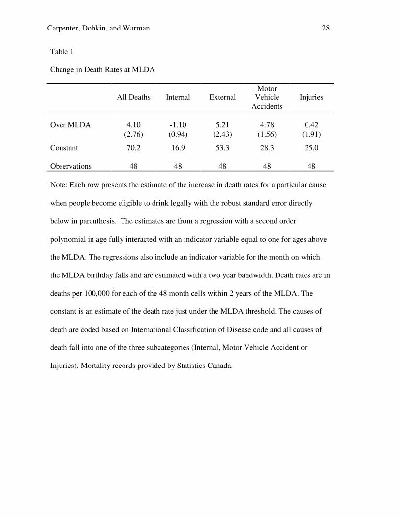
In Table 1 we present the point estimates of the change in death rates that occurs at the
MLDA that correspond to the age profiles in Figure 1. The estimate of the change in death rates
is presented with its standard error directly below, and these models include an indicator variable
for the MLDA-birthday month to account for celebration effects. Because the polynomial in age
in the regression has been re-centered at the MLDA, the constant provides an estimate of the
death rate immediately before people are legally of age to drink. The regression results for
motor vehicle mortality in the fourth column of Table 1 reveal that the increase in motor vehicle
deaths visible in the age profiles in Figure 1 is about 4.8 deaths per 100,000 person years at the
MLDA on a base of 28.3 (i.e., a 17 percent increase) and that this is statistically significant.
Column 2 shows that – consistent with the age profile in Figure 1 – the estimates of the change
in deaths due to internal causes is small and statistically insignificant. Column 5 of Table 1
shows that the estimated effect of the MLDA on deaths due to injuries other than motor vehicle

Carpenter, Dobkin, and Warman 11
accidents is also small and statistically significant, such that the RD estimate on total external
deaths (5.21 deaths per 100,000 person years) is similar to the baseline MVA estimate and is
statistically significant. The estimated increase in total deaths in column 1 of Table 1 is
approximately the same size as the increase in motor vehicle fatalities at the MLDA (though it is
not statistically significant), suggesting that deaths due to MVAs are driving the majority of the
overall increase in mortality.19
Notably, the estimated effect sizes for Canada are very similar to
those estimated previously using this same design in the US.
We next examine how the mortality effects of the MLDA vary by gender in Figures 2 and
3. Figure 2 reveals that young men in this age range have much higher death rates than women
and that there is an increase in their MVA-related death rates at the MLDA. A close examination
of the corresponding age profiles for women in Figure 3 reveals no compelling evidence of a
change in mortality rates at the MLDA for any cause of death. In Table 2 we present the
regression estimates of the changes in death rates at the MLDA by gender. These estimates
confirm that the increase in motor vehicle accident mortality is much larger for men compared to
women – 7.3 additional deaths per 100,000 for men with only 2.1 additional deaths per 100,000
for women – and the estimate is only statistically significant for men.20
In Appendix 5 we
present estimates of the mortality effect at bandwidths from 0.75 years to 3 years for men. The
figure reveals that the estimate of the effect of the MLDA on motor vehicle fatalities is
statistically significant throughout the entire range of bandwidths for men and that the other two
causes of death are not significant at conventional levels at all but one point. The corresponding
robustness analysis for women in Appendix 6 reveals that for all three causes of death the
estimate of the mortality effect is consistently much smaller and statistically insignificant
through almost the entire range of bandwidths. These results suggest that any alcohol
Carpenter, Dobkin, and Warman 12
consumption mechanisms underlying the mortality effect of the MLDA ought to exhibit a strong
gender differential consistent with the gender-specific mortality effects observed above.21
B. Descriptive Evidence – Alcohol Consumption
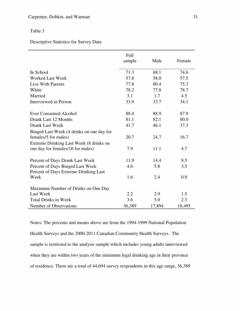
Before turning to RD evidence on the effect of the MLDA on drinking behaviors, we first
present some basic demographic information about the sample of young adults surveyed when
they are within two years of the MLDA in their province of residence. These patterns are
presented in Table 3 and reveal that the majority of the sample reports that they work and that
they live at home. The differences across gender are small with women being slightly more
likely to be in school and slightly less likely to live at home. When we examine the patterns of
alcohol consumption we find that 88 percent of young adults report having consumed alcohol at
some point in their lives and 81 percent report drinking in the past year; this differs little across
gender. In contrast, gender differences are very apparent when we examine measures that reflect
the frequency or intensity of alcohol consumption. For frequency of past week drinking men
report drinking on 14.4 percent of days and women on 9.5 percent. There is a similar pattern for
binge drinking and extreme drinking with more men reporting they drink at these intensities and
that they do so more frequently than women. The remaining rows of Table 3 show that by all
measures young males drink more heavily than young females.
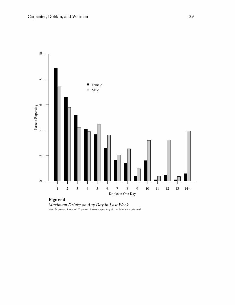
To more fully characterize the gender differences in drinking intensity, in Figure 4 we
present a histogram of the maximum number of drinks a person reports consuming on any single
day in the last week for the same sample of respondents as are included in Table 3. To put the
histogram in a scale that is easier to examine we suppress the set of bars corresponding to people
that report not drinking in the last week (54 percent of men and 63 percent of women). The
figure reveals that many young adults are engaging in extreme drinking. Over 11 percent of
Carpenter, Dobkin, and Warman 13
males report consuming at least 10 drinks on a single day (which is twice the threshold for binge
drinking for males) in the week prior to interview, and almost 4 percent of male respondents
report consuming 14 or more drinks on at least one day in the prior week. Among young women
in our sample extreme drinking is less common but still nontrivial: almost 5 percent of females
report consuming 8 or more drinks on a single day in the prior week (again, twice the threshold
for binge drinking for females). To our knowledge, this is the first large-scale evidence on the
extent of this ‘extreme’ drinking behavior using population-representative surveys.
C. Results on the MLDA and Alcohol Consumption in Canada
In this section we comprehensively document how alcohol consumption responds to the
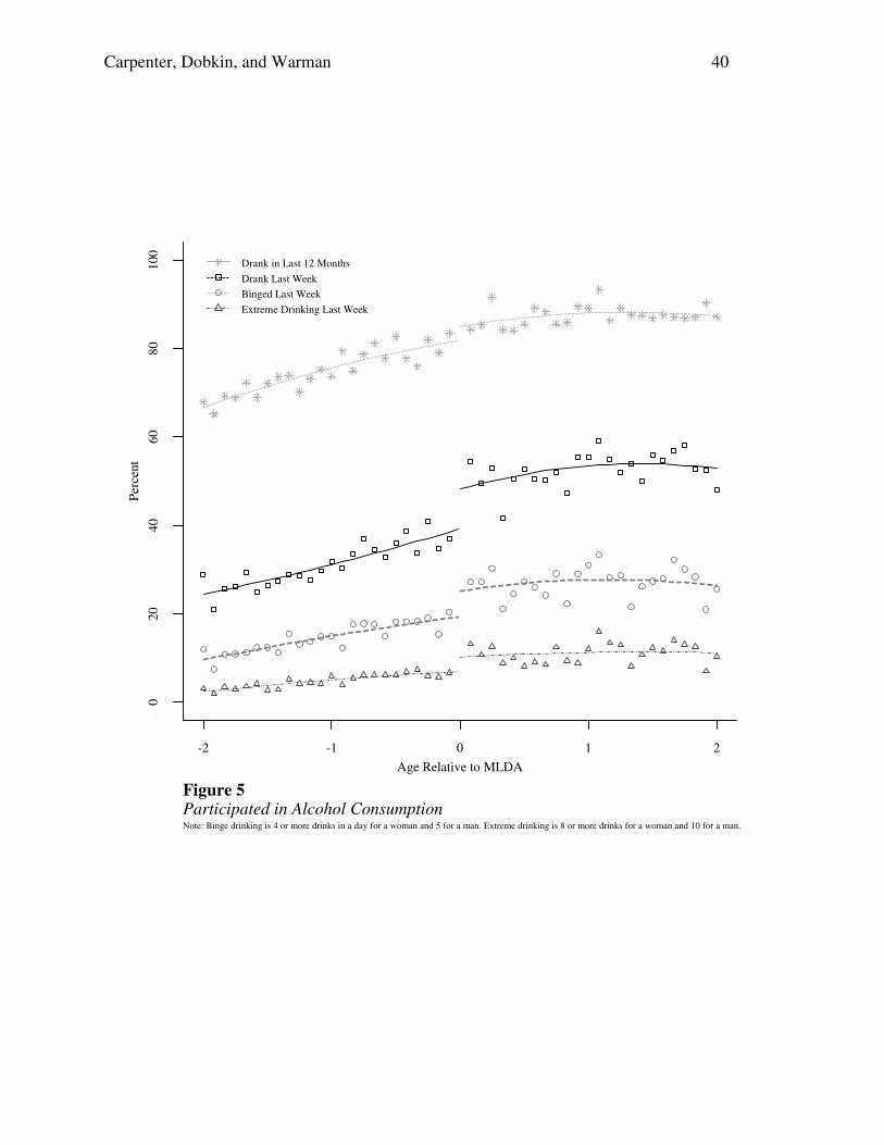
MLDA in Canada, using information on the full distribution of drinking. We begin with Figure
5 which presents age profiles for key measures of alcohol consumption in our data that are the
closest to those that have been examined in prior work: the percent of respondents reporting any
drinking in the past twelve months, the percent reporting any drinking in the past week, and the
percent reporting any binge drinking in the past week. We have also included the age profile of
extreme drinking which we are able to estimate due to the detailed questions on alcohol
consumption in the Canadian surveys. To make the age profile less noisy the percentages have
been calculated for 30 day blocks of age rather than for age in days (though the regressions use
exact age in days). Over these age profiles we have superimposed the fitted lines from a
regression on the underlying microdata that includes a quadratic polynomial in age fully
interacted with an indicator variable for being over the provincial drinking age.
Figure 5 reveals that about 40 percent of youths below their provincial MLDA report
having consumed alcohol in the past week and that there is evidence of a discontinuous increase
at the MLDA of about 8 percentage points. There is also a discrete jump in binge drinking of

Carpenter, Dobkin, and Warman 14
around 5 percentage points and a discrete jump in extreme drinking of 2-3 percentage points.
However, there is not much evidence of a discontinuity at the MLDA for past year drinking
participation, suggesting that the MLDA does not restrict people from having their first exposure
to alcohol. In Figure 6 we present the age profiles of several measures of the intensive margin of
drinking. The figure reveals that at the MLDA there are discernible increases in the proportion
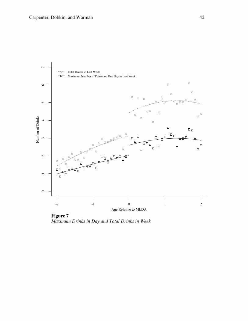
of days on which people engage in drinking, binge drinking, and extreme drinking. Figure 7
contains age profiles of the total number of drinks consumed in the past week and the maximum
number of drinks the individual reports consuming on any one day in the past week. Here too
we find strong evidence that these previously unstudied measures of alcohol consumption
increase significantly at the MLDA.
In Table 4 we present the point estimates of the discrete changes in the various alcohol
consumption measures we observe in Figures 5-7. Each entry is the coefficient on the indicator
variable for being over the MLDA which is our estimate of the discrete change in alcohol
consumption at the MLDA with its standard error directly below it in parenthesis. For the
regressions where the dependent variable is either a proportion or binary, the point estimates and
the standard errors have been multiplied by 100. We cluster standard errors on day of age
relative to the provincial drinking age. We present estimates without covariates in the top panel,
and in the bottom panel we present the same regressions with a rich set of covariates added. The
addition of covariates has a very small impact on the point estimates, suggesting that the
covariates are uncorrelated with the indicator variable for being over the MLDA in regressions
that condition on a quadratic polynomial in age. The covariates do predict alcohol consumption
as can be inferred from the fact that their inclusion slightly reduces the size of the standard errors
for a number of the point estimates.

Carpenter, Dobkin, and Warman 15
The results in Table 4 confirm the visual evidence from Figures 5-7. We focus on the
results in the bottom panel of the table as these are the ones with the covariates included.22
We
first confirm that the increase in past year drinking is small and statistically insignificant: the
estimate in the bottom panel of the first column suggests that past year drinking increases by
three percentage points at the MLDA, or less than four percent relative to the average past year
drinking rate of youths just under their provincial MLDA (confirming the very small visual
increase in Figure 5). In contrast, we estimate that the likelihood a young adult reports drinking
any alcohol in the past week increases by about 8 percentage points at the MLDA, and this
estimate is statistically significant.23
Relative to the drinking rate of youths just under their
provincial MLDA, this is about a 22.9 percent increase. Taken together, these two estimates
highlight the importance of the very recent alcohol consumption information in the CCHS and
suggest that the longer reference windows more common in US datasets are likely to bias down
estimates of the effect of the MLDA on drinking.
Table 4 also shows that the probability of binge drinking in the last week increases at the
MLDA by about 5.0 percentage points, or by about 29 percent relative to the rate for youths just
below the MLDA. We see that proportion of the population participating in extreme drinking
increases at the MLDA by 2.7 percentage points, or by about 44 percent relative to the rate for
youths just below the MLDA. There is also a discernible and statistically significant increase in
the frequency of binge drinking and extreme drinking at the MLDA.24
Finally, for all the
outcomes there is a very large celebration effect. This is documented in the second row of each
panel which presents the coefficient on the indicator variable for having been surveyed on a date
for which the relevant reference window includes the respondent’s MLDA-birthday.25

Carpenter, Dobkin, and Warman 16
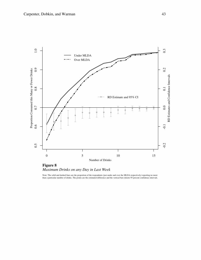
We summarize the changes in the drinking participation in Figure 8, which shows an
estimate of the cumulative distribution function of the maximum number of drinks consumed on
a single day in the past week for youths just under the MLDA (solid line) and youths just over
the MLDA (dashed line). The two cumulative distribution functions are estimated using the
same regression discontinuity approach as is used in the rest of the paper. The vertical distance
between these two lines is presented by the dot (as scaled by the right y-axis) with its 95 percent
confidence interval. These dots are the RD estimates of the effect of the MLDA on each level of
drinking intensity [i.e., the causal effect of the easier alcohol access on the likelihood the
individual reports consuming less than that number of drinks on every day in the past week].
When the two lines lie on top of each other (as they do at or near 12 drinks consumed on a single
day), there is no meaningful difference in population level drinking behavior at that point in the
maximum-drinks-on-a-single-day distribution – and thus the RD estimates are near zero and
statistically insignificant. The patterns in Figure 8 confirm those in Figure 5 and Table 4 and
demonstrate that looking only at past week drinking and binge drinking behavior misses
important effects of the MLDA which occur much higher in the drinks distribution than at the
binge drinking threshold. Specifically, while there is evidence of discontinuities for at least 1
and at least 4 or 5 drinks on a single day (equivalent to past week drinking participation and past
week binge drinking), there is also evidence of increases at levels up to 10 drinks.26
Several additional analyses suggest that the MLDA effects on drinking that we identify
are robust. For example, Figures 5-7 indicate that the choice of polynomial order is appropriate,
as the regression lines fit the age profiles well. Also, the fact that as documented in Table 4 the
inclusion of covariates does not significantly affect the point estimates is indirect evidence that
the quadratic polynomial is sufficiently flexible to absorb the changes in peoples’ circumstances
Carpenter, Dobkin, and Warman 17
that are occurring with age (such as changes in employment status or school attendance) and that
there are no sharp changes in these factors at the MLDA. As more direct evidence in Table 5 we
present estimates of the change in sample characteristics at the MLDA including: working,
school attendance, living at home and marital status. We do not find evidence of statistically
significant changes in any of these variables, further suggesting that our RD estimates of the
effect of the MLDA on drinking outcomes are not confounded by systematic changes in
unobserved characteristics at the relevant threshold. The last column of Table 5 also reports
evidence that there is no discontinuous change in the number of people interviewed at the
provincial MLDA threshold, in the spirit of the McCrary (2008) density test.
D. Drinking Results Stratified by Gender
The analysis above reveals that the MLDA affects multiple margins of drinking behavior.
This is one of the main challenges to pinpointing the mechanisms of alcohol control: because so
many different drinking outcomes exhibit significant discontinuities at the MLDA, the various
mechanisms that may plausibly contribute to the mortality effects are empirically
indistinguishable from one another without a sharper comparison. Fortunately, the gender-
specific nature of the mortality effect of the MLDA provides us such a comparison. Specifically,
we estimated above that the mortality effect of the MLDA was large and statistically significant
for young males while it was much smaller and insignificant for young females.
Given this sharp gender difference, we next explore to what extent the various drinking
outcomes documented above exhibit gender-specific differences in the effects of the MLDA.
Table 6 presents these results.27
The table reveals that for most measures of alcohol
consumption, other than extreme drinking, women report larger increases at the MLDA than
men. This is despite the fact that women have lower baseline levels of drinking. For example,
Carpenter, Dobkin, and Warman 18
we estimate in Table 6 that the probability the individual reported any binge drinking in the prior
week increased by 7.1 percentage points for women, or by about 58.7 percent relative to the
binge drinking rate of young women just below the MLDA. In contrast, the estimate of the
effect of the MLDA on binge drinking probability for men is much smaller (2.6 percentage
points, or just 12 percent of the rate for young men just below the MLDA) and statistically
insignificant. The same pattern also holds true for the frequency of binge drinking in Table 6.
These results for binge drinking (and for drinking participation) are inconsistent with the gender-
specific mortality pattern documented above and cast doubt that binge drinking per se is the key
causal factor behind the fatality effects of the MLDA.
Further examination of Table 6, however, reveals that this gender-specific pattern is
exactly reversed for extreme drinking. That is, for extreme drinking we find large and
statistically significant increases in both participation rates and frequency of this type of drinking
behavior at the MLDA for men but find no evidence of increases in either measure of extreme
drinking for women. In fact, the point estimates of the effect of the MLDA for the two extreme
drinking outcomes for women are both zero.28
Taken together, the results in Table 6 suggest that
the MLDA prevents some moderate consumption of alcohol by both men and women with a
much larger impact on the moderate drinking of women. However, the starkest differences (and
the differences that exhibit the gender-specific pattern of mortality effects observed above) in the
impact of the MLDA appear to be higher in the distribution of drinking intensity where it
prevents a substantial amount of extreme drinking by young men.
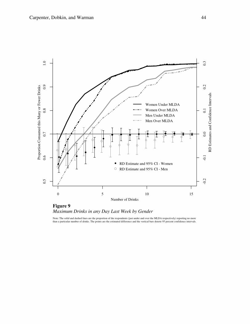
We demonstrate these gender-based differences more explicitly in Figure 9 which
presents estimates of the cumulative density function of maximum drinks consumed on a single
day in the past week and the associated RD estimates at each point in the maximum-drinks-on-a-

Carpenter, Dobkin, and Warman 19
single-day distribution by gender (i.e., Figure 9 presents Figure 8 separately by gender). The
figure reveals that for women the MLDA has a large effect on alcohol consumption up to about
five drinks in a day, but above this the MLDA has no effect.29
In contrast, the cdf of maximum
drinks consumed on a single day for men shows the MLDA has an estimated impact on alcohol
consumption up to 14 drinks in a day, though only the point estimates up to nine drinks per day
are statistically significant.30
Taken together, the gender differences in the effect of the MLDA
on alcohol consumption – in addition to providing new evidence on treatment effect
heterogeneity of the MLDA – provide evidence consistent with the idea that one key mechanism
of alcohol control in this context is the moderation of otherwise extreme drinking behavior.31
IV. Discussion and Conclusion
A substantial literature in health economics links stricter alcohol control policies to
reduced alcohol-related harms – especially motor vehicle mortality – but provides far less
evidence on the effect of the policies on alcohol consumption. Even less is known about what
types of reductions in alcohol consumption are causing the reduction in death rates. These gaps
are largely due to data limitations, which we rectify in this paper by examining the effect of the
MLDA in Canada on mortality and on the full distribution of alcohol consumption. We
document that – as in the US – motor vehicle accident mortality increases sharply at the MLDA
by about 17 percent. Important to our tests of alcohol consumption mechanisms, we show that
these effects are much larger and only statistically significant for men.
We then address the challenges of previous research in pinpointing mechanisms by taking
advantage of very detailed survey questions on alcohol consumption which allow us to map out
how the MLDA affects the entire distribution of alcohol consumption with respect to intensity

Carpenter, Dobkin, and Warman 20
and frequency of very recent drinking. We show that the MLDA has effects on moderate and
binge drinking that are as large or larger for women than for men. This is surprising given that
men have a larger increase in mortality rates, and it suggests that binge drinking alone is very
unlikely to be responsible for the mortality-reducing effects of the MLDA. In fact, we estimate
no significant effect of the MLDA on binge drinking, as defined in the public health literature,
among young men. Investigating further, however, we found that at the MLDA men increase
their extreme drinking much more substantially than women do. This – in combination with the
findings that men have much larger increases in fatality rates due to motor vehicle accidents then
women at the MLDA – is most consistent with the hypothesis that the MLDA reduces mortality
rates by reducing extreme drinking behavior among young men.
Importantly, our results are likely to inform a growing body of research on gender
differences in the effects of alcohol control policies generally and minimum drinking ages in
particular.32
For example, prior work using this same RD design for the United States also found
larger reduced form effects of the MLDA on mortality for young men compared to young
women (Carpenter and Dobkin 2009) and a similar gender-specific pattern for arrests (Carpenter
and Dobkin 2013, forthcoming), emergency room visits, and inpatient hospital admissions
(Carpenter and Dobkin 2014).33
If the drinking age in the US also works primarily to moderate
extreme drinking by young men, our results are also suggestive of an important role for extreme
drinking in morbidity, crime, and other acute alcohol-related harms.
Our results also have important implications for large scale survey design in the United
States and elsewhere that currently lack detailed questions on the distribution of drinks
consumed. Commonly used datasets such as the Centers for Disease Control’s Behavioral Risk
Factor Surveillance System and the National Centers for Health Statistics’ National Health
Carpenter, Dobkin, and Warman 21
Interview Survey should consider including more detailed questions about recent alcohol
consumption that more fully capture the distribution of drinking intensity. This would allow
researchers to more accurately characterize the prevalence, correlates, determinants, and effects
of extreme drinking behaviors throughout the US population. Our results suggest that failing to
do so may lead to incomplete and/or incorrect conclusions about the appropriate economic and
policy responses to curb problem drinking.
Overall these findings significantly advance our understanding of the alcohol
consumption mechanisms through which alcohol control reduces mortality rates and suggest that
policies designed to reduce acute alcohol-related harms should include a focus on curbing
extreme drinking.34
Since mortality is the largest social cost of youth drinking, these results also
suggest that the MLDA and other alcohol control policies that can reduce extreme drinking (as
opposed to lower intensities of drinking) are more likely to pass typical cost/benefit calculations.
In contrast, policies that primarily manipulate moderate drinking are less likely to be justifiable.
Carpenter, Dobkin, and Warman 22
References
Biderman, Ciro, Joao M P DeMello, and Alexandre Schneider. 2010. “Dry Laws and Homicides:
Evidence from the Sao Paulo Metropolitan Area.” Economic Journal 120(543): 157-82.
Boes, Stefan and Steven Stillman. 2013. “Does Changing the Legal Drinking Age Influence
Youth Behavior?” IZA Discussion Paper 7522.
Bonnie, Richard, and Mary Ellen O’Connell, eds. 2004. Reducing Underage Drinking: A
Collective Responsibility. Washington, DC: The National Academies Press.
CBC. 2012. “Sask. Party Members Vote to Lower Drinking Age.” CBC News, cbc.ca, updated
November 13, 2012 8:15pm. Available here:
http://news.ca.msn.com/local/saskatchewan/sask-party-members-vote-to-lower-drinking-age.
Calonico, Sebastian, Mattias Cattaneo, and Rocio Titiunik. 2014. “Robust Nonparametric
Confidence Intervals for Regression-Discontinuity Designs.” Econometrica. Forthcoming.
Carpenter, Christopher. 2004. “How Do Zero Tolerance Drunk Driving Laws Work?” Journal of
Health Economics. 23(1): 61-83.
Carpenter, Christopher and Carlos Dobkin. 2014. “The Minimum Drinking Age and Morbidity
in the US.” Working paper.
__________. 2013. “The Minimum Legal Drinking Age and Crime.” Review of Economics and
Statistics. Forthcoming.
__________. 2011. “The Minimum Legal Drinking Age and Public Health.” Journal of
Economic Perspectives. 25(2): 133-56.
__________. 2009. “The Effect of Alcohol Access on Consumption and Mortality: Regression
Discontinuity Evidence from the Minimum Drinking Age.” American Economic Journal:
Applied Economics. 1(1): 164-82.

Carpenter, Dobkin, and Warman 23
Carrell, Scott, Mark Hoekstra, and James West. 2011. “Does Drinking Impair College
Performance? Evidence from a Regression Discontinuity Approach.” Journal of Public
Economics. 95(1-2): 54-62.
Conover, Emily and Dean Scrimgeour. 2013. “Health Consequences of Easier Access to
Alcohol: New Zealand Evidence.” Journal of Health Economics. 32(3): 570-85.
Cook, Philip. 1981. “The Effect of Liquor Taxes on Drinking, Cirrhosis, and Auto Fatalities.” In
Alcohol and public policy: Beyond the shadow of prohibition, eds. Mark Moore and Dean
Gerstein, 255-85. Washington, DC: National Academies of Science.
Cook, Philip, and Michael Moore. 2001. “Environment and Persistence in Youthful Drinking
Patterns.” In Risky Behavior Among Youths: An Economic Analysis, ed. Jonathan Gruber,
375-437. Chicago: University of Chicago Press.
Cook, Philip, and George Tauchen. 1982. “The Effect of Liquor Taxes on Heavy Drinking.” The
Bell Journal of Economics. 13(2): 379-90.
__________. 1984. “The Effect of Minimum Drinking Age Legislation on Youthful Auto
Fatalities.” The Journal of Legal Studies. 13(1): 169-90.
Crost, Benjamin and Santiago Guerrero. 2012. “The Effect of Alcohol Availability on Marijuana
Use: Evidence from the Minimum Legal Drinking Age.” Journal of Health Economics,
31(1): 112-21.
Crost, Benjamin and Daniel Rees. 2013. “The Minimum Legal Drinking Age and Marijuana
Use: New Estimates from NLSY97.” Journal of Health Economics. 32(2): 474-76.
Dee, Thomas. 1999. “State Alcohol Policies, Teen Drinking and Traffic Fatalities.” Journal of
Public Economics. 72(2): 289-315.
Carpenter, Dobkin, and Warman 24
Edwards, Griffith, Peter Anderson, Thomas F. Babor, Sally Caswell, Roberta Ferrence, Norman
Geisbrecht, Christine Godfrey, Harold D. Holder, Paul H. M. M. Lemmens, Klaus Makela,
Lorraine T. Midanik, Thor Norstrom, Esa Ostrerberg, Anders Romelsjo, Robin Room, Jussi
Simpura, and Ole-Jorgen Skog, eds. 1994. Alcohol Policy and the Public Good. Oxford:
Oxford University Press.
Eisenberg, Daniel. 2003. “Evaluating the Effectiveness of Policies Related to Drunk Driving.”
Journal of Policy Analysis and Management. 22(2): 249-74.
Geisbrecht, Norman, Timothy Stockwell, Perry Kendall, Robert Strang, and Gerald Thomas.
2011. “Alcohol in Canada: Reducing the Toll Through Focused Interventions and Public
Health Policies.” Canadian Medical Association Journal. 183(4): 450-55.
Grant, Darren. 2010. “Dead on Arrival: Zero Tolerance Laws Don’t Work.” Economic Inquiry.
49(2): 474-88.
Imbens, Guido and Karthik Kalyanaraman. 2012. “Optimal Bandwidth Choice for the
Regression Discontinuity Estimator.” Review of Economic Studies. 79(3): 933-59.
Imbens, Guido and Thomas Lemieux. 2008. “Regression Discontinuity Designs: A Guide to
Practice.” Journal of Econometrics. 142(2): 615-35.
Kenkel, Donald S. 1995. “Drinking, Driving, and Deterrence: The Effectiveness and Social
Costs of Alternative Policies.” Journal of Law and Economics. 36(2): 877-913.
Kreft, Steven F. and Nancy M. Epling. 2007. “Do Border Crossings Contribute to Underage
Motor-Vehicle Fatalities? An Analysis of Michigan Border Crossings.” Canadian Journal of
Economics. 40(3): 765-81.
Lee, David, and Thomas Lemieux. 2010. “Regression Discontinuity Designs in Economics.”
Journal of Economic Literature. 48(2): 281-355.

Carpenter, Dobkin, and Warman 25
Levitt, Steven D. and Jack Porter. 2001. “How Dangerous are Drinking Drivers?” Journal of
Political Economy. 109(6): 1198-237.
Lindo, Jason, Peter Siminski, and Oleg Yerokhin. 2013. “Breaking the Link Between Legal
Access to Alcohol and Motor Vehicle Accidents: Evidence from New South Wales.”
Working paper.
Lindo, Jason, Isaac Swenson, and Glenn Waddell. 2013. “Alcohol and Student Performance:
Estimating the Effect of Legal Access.” Journal of Health Economics. 32(2013): 22-32.
Lovenheim, Michael and Joel Slemrod. 2010. “The Fatal Toll of Driving to Drink: The Effect of
Minimum Legal Drinking Age Evasion on Traffic Fatalities.” Journal of Health Economics.
29(1): 62-77.
Lovenheim, Michael and Daniel Steefel. 2009. “Do Blue Laws Save Lives? The Effect of
Sunday Alcohol Sales Bans on Fatal Vehicle Accidents.” Journal of Policy Analysis and
Management. 30(4): 798-820.
McCrary, Justin. 2008. “Manipulation of the Running Variable in the Regression Discontinuity
Design: A Density Test.” Journal of Econometrics. 142(2): 698-714.
Nelson, Jon P. 2014. “Binge Drinking, Alcohol Prices, and Alcohol Taxes: A Systematic Review
of Results for Youth, Young Adults, and Adults from Economic Studies, Natural
Experiments, and Field Studies.” SSRN Working Paper 2407019.
__________. 2013. “Gender Differences in Alcohol Demand: A Systematic Review of the Role
of Prices and Taxes.” Health Economics. Forthcoming.
Rehm, Jurgen. 1998. “Measuring Quantity, Frequency, and Volume of Drinking.” Alcoholism:
Clinical and Experimental Research. 22(2) April Supplement: 4S-14S.
Carpenter, Dobkin, and Warman 26
Seidl, Stephan, Uwe Jensen, and Andreas Alt. 2000. “The Calculation of Blood Ethanol
Concentrations in Males and Females.” International Journal of Legal Medicine. 114(1–2):
71–7.
Sloan, Frank, Bridget Reilly, and Chrostph Schenzler. 1995. “Effects of Tort Liability and
Insurance on Heavy Drinking and Drinking and Driving.” Journal of Law and Economics.
38(1): 49-78.
Stabile, Mark, Audrey Laporte, and Peter C. Coyte. 2006. “Household Responses to Public
Home Care Programs.” Journal of Health Economics. 25(4): 674-701.
Stehr, Mark. 2010. “The Effect of Sunday Sales of Alcohol on Highway Crash Fatalities.” BE
Journal of Economic Analysis and Policy. 10(1).
Stockwell, Tim, Susan Donath, Mark Cooper-Stanbury, Tany Chikritzhs, Paul Catalon, and Cid
Mateo. 2004. “Under-reporting of Alcohol Consumption in Household Surveys: A
Comparison of Quantity-Frequency, Graduated-Frequency, and Recent Recall.” Addiction.
99(8): 1024-33.
Stockwell, Tim, Jinhui Zhao, Tanya Chikritzhs, and Tom K. Greenfield. 2008. “What Did You
Drink Yesterday? Public Health Relevance of a Recent Recall Method Used in the 2004
Australian National Drug Strategy Household Survey.” Addiction. 103(6): 919-28.
Thistlewaite, Donald, and Donald Campbell. 1960. “Regression-Discontinuity Analysis: An
Alternative to the Ex Post Facto Experiment.” Journal of Educational Psychology. 51: 309-
17.
Vingilis, Evelyn and Reginald Smart. 1981. “Effects of Raising the Legal Drinking Age in
Ontario.” British Journal of Addiction. 76(4): 415-24.

Carpenter, Dobkin, and Warman 27
Wagenaar, Alexander C and Traci L. Toomey. 2002. “Effects of Minimum Drinking Age Laws:
Review and Analyses of the Literature from 1960 to 2000.” Journal of Studies on Alcohol.
Supplement 14: 206-25.
Wechsler, Henry and Toben Nelson. 2006. “Relationship Between Level of Consumption and
Harms in Assessing Drink Cut-Points for Alcohol Research: Commentary on ‘Many College
Freshmen Drink at Levels Far Beyond the Binge Threshold’ by White et al.” Alcoholism:
Clinical and Experimental Research. 30(6): 922-27.
__________. 2001. “Binge Drinking and the American College Student: What’s Five Drinks?”
Psychology of Addictive Behaviors. 15(4): 287-91.
White, Aaron M., Courtney L, Kraus, and Harry Scott Swartzwelder. 2006. “Many College
Freshmen Drink at Levels Far Beyond the Binge Threshold.” Alcoholism: Clinical and
Experimental Research. 30(6): 1006-10.
Carpenter, Dobkin, and Warman 28
Table 1
Change in Death Rates at MLDA
All Deaths Internal External
Motor
Vehicle
Accidents
Injuries
Over MLDA 4.10 -1.10 5.21 4.78 0.42
(2.76) (0.94) (2.43) (1.56) (1.91)
Constant 70.2 16.9 53.3 28.3 25.0
Observations 48 48 48 48 48
Note: Each row presents the estimate of the increase in death rates for a particular cause
when people become eligible to drink legally with the robust standard error directly
below in parenthesis. The estimates are from a regression with a second order
polynomial in age fully interacted with an indicator variable equal to one for ages above
the MLDA. The regressions also include an indicator variable for the month on which
the MLDA birthday falls and are estimated with a two year bandwidth. Death rates are in
deaths per 100,000 for each of the 48 month cells within 2 years of the MLDA. The
constant is an estimate of the death rate just under the MLDA threshold. The causes of
death are coded based on International Classification of Disease code and all causes of
death fall into one of the three subcategories (Internal, Motor Vehicle Accident or
Injuries). Mortality records provided by Statistics Canada.

Carpenter, Dobkin, and Warman 29
Table 2
Change in Death Rates at MLDA by Gender
All Deaths Internal External
Motor
Vehicle
Accidents
Injuries
Male
Over MLDA 6.91 -3.95 10.86 7.32 3.54
(5.15) (2.24) (4.56) (2.63) (3.20)
Constant 103.5 21.2 82.34 43.3 39.0
Female
Over MLDA 1.14 1.89 -0.75 2.12 -2.86
(2.29) (1.58) (1.70) (1.17) (1.36)
Constant 35.2 12.5 22.70 12.5 10.2
p-value of
difference
in effect by
gender 0.309 0.036 0.019 0.074 0.069
Note: Each row presents the estimate of the increase in death rates for a particular cause
when people become eligible to drink legally with the robust standard error of the estimate
directly below in parenthesis. The estimates are from a regression with a second order
polynomial in age fully interacted with an indicator variable equal to one for ages above the
MLDA. The regressions also include an indicator variable for the month on which the
MLDA birthday falls and are estimated with a two year bandwidth. Death rates are in
deaths per 100,000 for each of the 48 month cells within 2 years of the MLDA. The
constant is an estimate of the death rate just under the MLDA threshold. The causes of
death are coded based on International Classification of Disease code and all causes of
death fall into one of the three subcategories (Internal, Motor Vehicle Accident or Injuries).
Mortality records provided by Statistics Canada. In the bottom row we present the p-value

Carpenter, Dobkin, and Warman 30
of the difference in the estimates of the MLDA effect.
Carpenter, Dobkin, and Warman 31
Table 3
Descriptive Statistics for Survey Data
Full
sample Male Female
In School 71.3 68.1 74.6
Worked Last Week 57.8 58.0 57.5
Live With Parents 77.8 80.4 75.3
White 78.2 77.8 78.7
Married 3.1 1.7 4.5
Interviewed in Person 33.9 33.7 34.1
Ever Consumed Alcohol 88.4 88.9 87.9
Drank Last 12 Months 81.1 82.1 80.0
Drank Last Week 41.7 46.1 37.3
Binged Last Week (4 drinks on one day for
females/5 for males) 20.7 24.7 16.7
Extreme Drinking Last Week (8 drinks on
one day for females/10 for males) 7.9 11.1 4.7
Percent of Days Drank Last Week 11.9 14.4 9.5
Percent of Days Binged Last Week 4.6 5.8 3.5
Percent of Days Extreme Drinking Last
Week 1.6 2.4 0.9
Maximum Number of Drinks on One Day
Last Week 2.2 2.9 1.5
Total Drinks in Week 3.6 5.0 2.3
Number of Observations 36,389 17,894 18,495
Notes: The percents and means above are from the 1994-1999 National Population
Health Surveys and the 2000-2011 Canadian Community Health Surveys. The
sample is restricted to the analysis sample which includes young adults interviewed
when they are within two years of the minimum legal drinking age in their province
of residence. There are a total of 44,694 survey respondents in this age range, 36,389
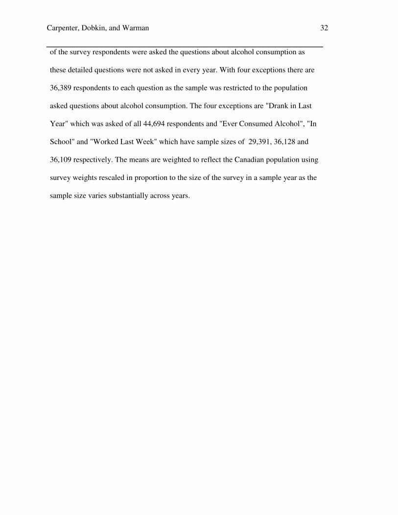
Carpenter, Dobkin, and Warman 32
of the survey respondents were asked the questions about alcohol consumption as
these detailed questions were not asked in every year. With four exceptions there are
36,389 respondents to each question as the sample was restricted to the population
asked questions about alcohol consumption. The four exceptions are "Drank in Last
Year" which was asked of all 44,694 respondents and "Ever Consumed Alcohol", "In
School" and "Worked Last Week" which have sample sizes of 29,391, 36,128 and
36,109 respectively. The means are weighted to reflect the Canadian population using
survey weights rescaled in proportion to the size of the survey in a sample year as the
sample size varies substantially across years.

Carpenter, Dobkin, and Warman 33
Table 4
Change in Drinking at MLDA
Drank
Last 12
Months
Drank
Last
Week
Binged
Last
Week
Extreme
Drinking
Last
Week
Percent
of Days
Drank
Last
Week
Percent
of Days
Binged
Last
Week
Percent
of Days
Extreme
Drinking
Last
week
Max
Drinks
in One
Day
Last
Week
Total
Drinks
in Last
Week
No Controls other than Birth
week
Over MLDA 3.7 8.3 5.0 2.5 3.7 1.8 0.5 0.48 1.17
(1.9) (2.5) (1.9) (1.3) (0.9) (0.5) (0.3) (0.18) (0.35)
Week after 1.6 20.0 17.7 12.3 6.7 3.6 2.7 1.96 2.96
Birthday (2.9) (5.2) (4.1) (4.3) (2) (1.1) (1) (0.56) (0.89)
Constant 81.5 38.9 19.1 6.9 10.2 3.9 1.4 2.00 3.10
(1.5) (1.6) (1.2) (0.7) (0.5) (0.3) (0.2) (0.1) (0.2)
Full set of controls
Over MLDA 2.9 8.0 5.0 2.7 3.5 1.8 0.5 0.48 1.16
(1.7) (2.4) (1.8) (1.2) (0.9) (0.5) (0.3) (0.17) (0.34)
Week after 2.6 19.6 17.4 12.1 6.7 3.5 2.7 1.94 2.93
Birthday (2.8) (4.7) (3.8) (4.2) (1.7) (1.1) (1) (0.54) (0.85)
Mean 78.8 34.9 17.0 6.1 9.2 3.6 1.3 1.77 2.81
Observations 44,694 36,389 36,389 36,389 36,389 36,389 36,389 36,389 36,389
Note: See notes for Table 3 for a description of the sample. All regressions include a second order
polynomial in age fully interacted with an indicator variable that takes on a value of 1 for people
interviewed when they are older than the MLDA. The estimates in the top row of each panel in the
table are for the coefficients on this indicator variable with its standard error directly below in
parenthesis. The regressions also include an indicator variable that takes on a value of one if the person
is interviewed in the week immediately after the birthday on which they become eligible to drink
legally. This is intended to absorb the pronounced "celebration" effects noticeable in the age profiles

Carpenter, Dobkin, and Warman 34
and is presented in the second major row of each panel. For the binary outcome variables the point
estimates and their SE have been multiplied by 100 to make them easier to read and interpretable as
percentage points. The standard errors are clustered on the running variable. The regressions are
weighted to account for the sampling frame. Extreme drinking is 8 or more drinks in a day for women
and 10 or more drinks in a day for men. The regressions in the bottom panel include controls for year
of survey, province of residence, white, marital status, living with parents, interview in person, in
school, work last week, gender, month of interview, and dummies flagging when in school or work
last week are missing. The means on the second to last row are for the subsample of people
interviewed when they are within one year of reaching the provincial MLDA.

Carpenter, Dobkin, and Warman 35
Table 5
Change in Sample Characteristics at MLDA
Interview
in Person
Work
Last
Week
In
School
Live
With
Parents Married Male White
Number of
People
Interviewed
Over MLDA -2.46 0.46 1.84 3.94 -1.34 0.57 0.03 1.09
(2.19) (2.43) (2.3) (2.08) (0.7) (2.57) (2.45) (1.24)
Constant 37.7 60.2 65.7 75.8 3.1 50.5 78.1 23.5
Observations 36,389 36,019 36,128 36,389 36,389 36,389 36,389 1,439
Notes: The point estimates of the discrete change at the MLDA are in percentage terms, with the
exception of the change in the number of people interviewed. For the number of people interviewed
the dependent variable is the number of people interviewed at a particular age in days. Standard
errors are in parenthesis below the point estimates. For details about the sample please see the notes
for Table 3 and for details on regression specifications please see the notes for Table 4. All
regressions include a second order polynomial in age fully interacted with an indicator variable that
takes on a value of 1 for people interviewed when they are older than the MLDA. The regressions
also include an indicator variable that takes on a value of one if the person is interviewed in the
week immediately after the birthday on which they become eligible to drink legally.

Carpenter, Dobkin, and Warman 36
-2 -1 0 1 2
Age Relative to MLDA
10
15
20
25
30
35
40
Dea
th R
ate
per
100,0
00
Motor Vehicle Accident
Injuries
Internal
Figure 1Age Profile of Mortality Rates by Cause

Carpenter, Dobkin, and Warman 37
-2 -1 0 1 2
Age Relative to MLDA
10
20
30
40
50
60
Dea
th R
ate
per
100,0
00
Motor Vehicle Accident
Injuries
Internal
Figure 2Age Profile of Mortality Rates - Men

Carpenter, Dobkin, and Warman 38
-2 -1 0 1 2
Age Relative to MLDA
05
10
15
20
25
30
Dea
th R
ate
per
100,0
00
Motor Vehicle Accident
Injuries
Internal
Figure 3Age Profile of Mortality Rates - Women
Carpenter, Dobkin, and Warman 39
1 2 3 4 5 6 7 8 9 10 11 12 13 14+
02
46
810
Drinks in One Day
Per
cent
Rep
ort
ing
Female
Male
Note: 54 percent of men and 63 percent of women report they did not drink in the prior week.
Figure 4Maximum Drinks on Any Day in Last Week
Carpenter, Dobkin, and Warman 40
-2 -1 0 1 2
Age Relative to MLDA
020
40
60
80
100
Per
cent
Drank in Last 12 Months
Drank Last Week
Binged Last Week
Extreme Drinking Last Week
Figure 5Participated in Alcohol ConsumptionNote: Binge drinking is 4 or more drinks in a day for a woman and 5 for a man. Extreme drinking is 8 or more drinks for a woman and 10 for a man.

Carpenter, Dobkin, and Warman 41
-2 -1 0 1 2
Age Relative to MLDA
05
10
15
20
Per
cent
of
Day
s in
Las
t W
eek
Drinking
Binge Drinking
Extreme Drinking
Figure 6Percent of Days Drinking Last WeekNote: Binge drinking is 4 or more drinks in a day for a woman and 5 for a man. Extreme drinking is 8 or more drinks for a woman and 10 for a man.
Carpenter, Dobkin, and Warman 42
-2 -1 0 1 2
Age Relative to MLDA
01
23
45
67
Num
ber
of
Dri
nks
Total Drinks in Last Week
Maximum Number of Drinks on One Day in Last Week
Figure 7Maximum Drinks in Day and Total Drinks in Week
Carpenter, Dobkin, and Warman 43
0 5 10 15
Number of Drinks
0.5
0.6
0.7
0.8
0.9
1.0
Pro
port
ion C
onsu
med
this
Man
y o
r F
ewer
Dri
nks
Under MLDA
Over MLDA
RD Estimate and 95% CI
-0.2
-0.1
0.0
0.1
0.2
0.3
RD
Est
imat
es a
nd C
onfi
den
ce I
nte
rval
sFigure 8Maximum Drinks on any Day in Last Week
Note: The solid and dashed lines are the proportion of the respondents (just under and over the MLDA respectively) reporting no more
than a particular number of drinks. The points are the estimated difference and the vertical bars denote 95 percent confidence intervals.
Carpenter, Dobkin, and Warman 44
0 5 10 15
Number of Drinks
0.5
0.6
0.7
0.8
0.9
1.0
Pro
port
ion C
onsu
med
this
Man
y o
r F
ewer
Dri
nks
Women Under MLDA
Women Over MLDA
Men Under MLDA
Men Over MLDA
RD Estimate and 95% CI - Women
RD Estimate and 95% CI - Men
-0.2
-0.1
0.0
0.1
0.2
0.3
RD
Est
imat
es a
nd C
onfi
den
ce I
nte
rval
sFigure 9Maximum Drinks in any Day Last Week by Gender
Note: The solid and dashed lines are the proportion of the respondents (just under and over the MLDA respectively) reporting no more
than a particular number of drinks. The points are the estimated difference and the vertical bars denote 95 percent confidence intervals.
Carpenter, Dobkin, and Warman 45
1 Arguably the first to do so using modern quasi-experimental methods is Cook and Tauchen
(1982), who demonstrate that alcohol tax increases reduce death rates from liver cirrhosis.
2 Our paper focuses on young adults in Canada between the ages of 16 and 19 in Alberta,
Manitoba, and Quebec and between the ages of 17 and 20 in the rest of Canada. These are the
‘young men’, ‘young women’, and/or ‘young adults’ referenced in this paper.
3 Levitt and Porter (2001) provide novel evidence on the relative risk of drinking drivers using
information on two-car crashes. They find that drivers with any alcohol in their blood are seven
times more likely to cause a fatal crash, while drivers with a blood alcohol content (BAC) above
0.10 are 13 times more likely to cause a fatal crash.
4 The arbitrary nature of the binge drinking threshold (that is, 5 drinks for men and 4 drinks for
women) has been repeatedly criticized and debated by public health scholars. See, for example,
Wechsler and Nelson (2001); White et al. (2006); Wechsler and Nelson (2006); and others.
5 There are, of course, many other variables that affect the level of impairment at a particular
BAC; the description above is meant only as an illustrative example. Gender, body weight, body
composition/muscularity, and other factors all contribute to heterogeneity in these relationships.
6 Moreover, it is plausible that the broad range of alcohol control policies available to regulators
affect different parts of the drinking distribution in systematically different ways, further
increasing the latitude to match a specific alcohol control policy to a particular alcohol-related
harm. For example, it is possible that ‘aggravated’ drunk driving laws – which impose
additional sanctions at BACs above 0.15 and are being adopted by states in the US – affect a
different part of the distribution of drinking than do other types of alcohol control policies such
as taxes. This is an important area for future work.

Carpenter, Dobkin, and Warman 46
7 Alberta, Manitoba, and Quebec all have an MLDA of 18. The rest of Canada has an MLDA of
19. These MLDAs have been constant since the late 1970s, though recently some provinces
have actively considered lowering their MLDA (CBC 2012). The ‘age of majority’ for other
rights and responsibilities of adulthood also varies across provinces, but it does not exactly
coincide with the provincial MLDA (e.g., the age of majority in Ontario is 18 but its provincial
MLDA is 19). An exception to provincial variation in minimum ages for various rights is
voting: 18 is the minimum voting age throughout Canada. Importantly, the minimum age for
obtaining a driving permit in Canada varies across provinces but is several years lower than the
minimum drinking age (typically 14 or 16, depending on the province). Thus, we are not aware
of any rights or responsibilities of adulthood that should affect the outcomes we study in a
discontinuous way at the provincial MLDA other than easier access to alcohol. We combine all
provinces for the analyses in this paper; separate analyses by provincial MLDA are not
informative because the vast majority of the Canadian population resides in provinces with an
MLDA of 19. We revisit this issue below.
8 This design has been used recently to examine the effects of easier alcohol access on: marijuana
consumption (Crost and Guerrero 2012), academic outcomes of students at the United States
Military Academy (Carrell, Hoekstra, and West 2011), and academic outcomes of students at the
University of Oregon (Lindo, Swenson, and Waddell 2013), among others. It has also been used
to study the link between easier access to alcohol and health outcomes in Australia (Lindo,
Siminski, and Yerokhin 2013) and New Zealand (Conover and Scrimgeour 2013; Boes and
Stillman 2013).
9 We do not provide a detailed literature review on the effects of stricter alcohol controls on
motor vehicle accident mortality and other adverse events for youths. For a broad review of

Carpenter, Dobkin, and Warman 47
alcohol control policies and youth outcomes, see Cook and Moore (2001) and Wagenaar and
Toomey (2002). For pre-post evaluations of Canada’s MLDAs on outcomes, see Vingilis and
Smart (1981) and Kreft and Epling (2007).
10 Canada’s most populated province (Ontario) changed its MLDA in 1979 from 18 to 19, which
is why we begin in 1980 (the data are available back to 1974). There are not enough data from
1974-1979 to separately analyze the earlier period. Prince Edward Island changed its MLDA in
July 1987 from 18 to 19, so we analyze data from July 1988 (allowing for one year of
grandfathering) to 2008 for that province. Over our sample period other provincial alcohol
control policies and characteristics changed as well, including: increased outlet density,
imposition of minimum alcohol pricing, and stricter (i.e., lower) blood alcohol content
requirements for impaired driving (see Geisbrecht et al. 2011 for a discussion). Liquor
privatization also increased over our sample period, though Canada’s alcohol distribution sytem
is still characterized by much greater government involvement than in most of the United States.
We assume that these policies do not directly affect the discontinuity in drinking or mortality we
study, though they are important to keep in mind for generalizability and interpretation purposes.
11 The death certificates also include information on province of death, which matches province
of residence in the vast majority of cases. We use province of residence for our baseline
analyses to match the first stage results on alcohol consumption (which are based on the
respondent’s province of residence). Border crossing to lower-age provinces is mainly relevant
for Ottawa, which is located in Ontario (with an age-19 MLDA) but is right on the border with
Quebec (which has an age-18 MLDA). We obtained very similar results when we excluded
individuals residing in border towns to lower-age provinces.

Carpenter, Dobkin, and Warman 48
12
For an example of other research that uses these data in a similar fashion, see Stabile et al.
(2006).
13 The drinking related questions became optional questions (used only by certain provinces) in
2007-2011.
14 The surveys standardize what constitutes a drink. Specifically, the questionnaire asks: “When
we use the word ‘drink’ it means: one bottle or can of beer or a glass of draft; one glass of wine
or a wine cooler; one drink or cocktail with 1 and a 1/2 ounces of liquor”. Thus, while it is
possible that the type of beverage consumed changes discretely at the MLDA, total ethanol
consumption should be measured fairly accurately given the standardized ‘drink’ definition.
15 Alcohol researchers have used alcohol sales data to estimate that the amount of drinking is
underreported in surveys by 40 to 60 percent (Rehm 1998). Recent research, however,
demonstrates that the severity of underreporting of alcohol consumption is far lower in surveys
that ask about very recent drinking such as the CCHS (see, for example, Stockwell et al. 2004
and Stockwell et al. 2008).
16 To ensure that observations from smaller cycles are not overweighted, we normalize the
weights so that for each cycle the weights average to the sample size. Adjusted weights are
recalculated for each subsample.
17 This is equivalent to running a regression without a birthday indicator on a data set where the
observations that fall on the birthday or the week immediately after have been dropped and
recovering the estimate of the change in the outcome at the threshold by projecting over the
missing part of the age profile.
18 These categories are mutually exclusive and comprise all deaths. The injuries category
includes deaths due to falls, burns, drowning, and overdoses, among others. The sum of motor

Carpenter, Dobkin, and Warman 49
vehicle accident deaths and deaths due to injuries equals deaths due to external causes. We
provide a detailed list of the relevant ICD codes in Appendix 1.
19 Appendix 2 presents estimates from our preferred regression specification for bandwidths from
0.75 years to 3 years and shows that the point estimates are not sensitive to the choice of
bandwidth. Appendix 3 presents robustness of our main mortality results to linear and cubic
polynomials in relative age (our preferred specification uses a quadratic polynomial in relative
age); these results confirm that the MLDA patterns by cause of death are not sensitive to our
choice of polynomial. Appendix 4 presents the full set of coefficient estimates from our
preferred model for each cause of death.
20 We also present in Table 2 p-values for tests of equality of the coefficients by gender. Gender
differences in the effects of the MLDA on deaths due to external causes and motor vehicle
fatalities are statistically significant.
21 Appendix 7 presents robustness of our gender-specific mortality results to linear and cubic
polynomials in relative age (our preferred specification uses a quadratic polynomial in relative
age); these results confirm that the gender-specific MLDA patterns by cause of death are not
sensitive to our choice of polynomial. Appendix 8 presents the full set of coefficient estimates
by gender from our preferred model for each cause of death
22 We present expanded sets of coefficient estimates in Appendix 9. We also show robustness of
the full sample alcohol consumption models to controlling for linear and cubic polynomials in
relative age (instead of quadratic) in Appendix 10.
23 In results not reported but available upon request we also find that our main results are robust
to: restricting attention to the NPHS and CCHS cycles that include all provinces; restricting

Carpenter, Dobkin, and Warman 50
attention to respondents from Ontario (the only province observed in all waves); and estimating
the models without weights. These results are available upon request.
24 In Appendices 11-13 we present the RD estimates and confidence intervals for the key
drinking outcomes at every bandwidth between 0.25 and 3 years. These figures show that the
estimates are robust to choice of bandwidth.
25 Note that the effects on extreme drinking (and indeed all drinking outcomes) are net of the
celebration drinking effects, despite that much celebration drinking is likely to be extreme in
nature.
26 Appendix 14 presents the effects of the MLDA on the full distribution of drinking intensity in
a different way. Recall that people just under the MLDA report that on average they drank on 10
percent of days in the prior week and as documented in Table 4 this increases by 3.7 percentage
points at the MLDA. In Appendix 14 the hollow triangles (which are bracketed by their 95
percent confidence intervals) show the estimate of how this increase is distributed over the
different levels of drinking. In addition, as a baseline, the percent of days people report drinking
just prior to the MLDA are shown using solid triangles. The figure reveals very substantial
increases at the MLDA in the frequency of alcohol consumption up to a level of 12 drinks,
though at the higher level the estimates are somewhat imprecise.
27 The corresponding age profiles and fitted regressions are presented in Appendices 15-22.
Appendices 23 and 24 present the full set of coefficient estimates for the drinking outcomes for
males and females, respectively.
28 Table 6 also presents p-values for tests of equality of the effects of the MLDA on drinking
outcomes by gender and shows that the effects on both extreme drinking measures are
significantly different for young men compared to young women.

Carpenter, Dobkin, and Warman 51
29
In Appendix 25 we present the same contrast in terms of BAC computed using the formula
from Seidl et al. (2000) which adjusts for weight, height and gender. We also assume that all the
drinks are consumed over a 4 hour period though the results are qualitatively similar when we
assume the drinks are consumed at half hour intervals.
30 In Appendix 26 we present the percent of days on which men and women report each level of
drinking and how this changes at the MLDA (i.e., Appendix 26 presents Appendix 14 separately
by gender). This figure also reveals that men increase the percent of days on which they engage
in extreme drinking when they become eligible to drink legally.
31 We also explored other cuts of the consumption and mortality data, such as by provincial
MLDA and by weekday versus weekend. These alternative splits of the sample gave results
consistent with those that result from gender stratification, but they did not uniquely point to a
role for extreme drinking. That is, results by provincial MLDA or day of week exhibited effects
on drinking intensities that were often statistically significant but that could not adjudicate
among multiple possible alcohol consumption channels, which is the focus of the current
analysis. Limited statistical precision was also a challenge in these stratified models, particularly
for the mortality analyses. For completeness, we present these results in Appendices 27
(mortality, by provincial MLDA), 28 (consumption, by provincial MLDA), 29 (mortality, by
weekday/weekend), and 30 (consumption, by weekday/weekend). We also considered other
demographic cuts of the data besides gender; however, there are not enough nonwhites in the
Canadian sample to perform meaningful analyses by race, and there is no information on
education on the Canadian death certificate.
32 Multiple recent reviews of the evidence address the extent of gender differences in the effects
of alcohol prices and taxes on young adult drinking participation and binge drinking. Nelson

Carpenter, Dobkin, and Warman 52
(2013, 2014) finds that most studies show no responsiveness of binge drinking to prices or taxes
for either young men or young women, while there is some evidence that higher taxes reduce
drinking participation for young adults of both genders. In contrast, Carpenter (2004) finds that
age-targeted Zero Tolerance drunk driving laws had larger effects at reducing binge drinking of
young males compared to young females.
33 An exception is Conover and Scrimgeour (2013), who find very similar effects of a New
Zealand alcohol policy liberalization on male and female hospitalizations.
34 This contrasts with the population-level model of alcohol control advocated in Edwards et al.
(1994) which emphasizes policies such as higher taxes to reduce total alcohol consumption and
aggregate health costs of chronic alcohol use.

Appendix 1: ICD-9 and ICD-10 Codes Used to Create Cause-of-Deaths Categories ICD-9 ICD-10 MVA
‘81’, ‘820’, ’821’, ’822’, ’823’, ’824’, ‘825’
‘V0’,’ V1’, ’V2’, ’V3’, ’V4’, ’V5’, ’V6’, ’V7’, ‘V8’
Injuries
‘291’, ’303’, ’860’, ’3575’, ’4255’, ‘5353’, ’5710’, ’5711’, ’5712’, ’5713’, ‘7903’, '292', '304', '850', '851', '852', '853', '854', '855', '856', '857', '858', '3321', ‘3576’, '305', 95, 96
‘X6’, ’X7’, ’X80’, ’X81’, ’X82’, ’X83’, ‘X84’, ’X870’, ‘X85’, ’X86’, ’X87’, ’X88’, ’X89’, ’X9’, ‘Y0’, ‘F10’, ’K70’, ’X45’, ’X65’, ’Y15’, ’Y91’, ‘K70’, ’T51’, ’X46’, ’Y15’, ’Y90’, ‘Y91’, ’G312’, ’G621’, ’I426’, ’K292’, ‘R780’, ’E244’, ’G721’, ’K852’, ’K860’, ‘Z502’, ’Z714’, ’Z721’, ’K860’, ’T518’, ‘T519’, ‘F11’, ’F12’, ’F13’, ’F14’, ’F15’, ’F16’, ’F17’, ’F18’, ’F19’, ’F55’, ’T40’, ’T41’, ’T43’, ’F55’, ’X40’, ’X42’ and not in 'F116', 'F126', 'F136', 'F146', 'F156', 'F166', 'F176', 'F171', 'F172', 'F186', 'F196'
External MVA and Injuries MVA and Injuries Internal Everything else Everything else

● ●
●
●
●
●●
●
●● ●
●
● ●●
●● ● ●
●● ●
●● ●
● ●● ● ● ● ● ● ● ●
1.0 1.5 2.0 2.5 3.0Bandwidth in Years
−5
05
1015
Jum
p in
Dea
ths
at M
LDA
●
Motor Vehicle AccidentInjuryInternal
Appendix 2: Increase in Deaths at MLDA(Robustness to bandwidth choice )
Note: Regression estimates for every bandwidth between 1/4 year and 3 years. In the main specifications in the paper the bandwidth is 2 years.

Polynomial order 1 2 3 1 2 3 1 2 3 1 2 3 1 2 3
Over MLDA 5.83 4.10 10.73 0.20 -1.10 0.29 5.63 5.21 10.44 4.35 4.78 8.58 1.27 0.42 1.85(1.60) (2.76) (2.74) (0.63) (0.94) (1.55) (1.50) (2.43) (2.36) (0.95) (1.56) (2.01) (1.13) (1.91) (2.78)
Constant 71.1 70.2 68.5 16.2 16.9 17.2 54.9 53.3 51.3 29.1 28.3 26.9 25.7 25.0 24.4
Observations 48 48 48 48 48 48 48 48 48 48 48 48 48 48 48
Appendix 3: Change in Death Rates at MLDA
Note: Each row presents the estimate of the increase in death rates for a particular cause when people become eligible to drink legally with the robust standard error directly below in parenthesis. The estimates are from a regression with a first, second or third order polynomial respectively in age fully interacted with an indicator variable equal to one for ages above the MLDA. The regressions also include an indicator variable for the month on which the MLDA birthday falls and are estimated with a two year bandwidth. Death rates are in deaths per 100,000 for each of the 48 month cells within 2 years of the MLDA. The constant is an estimate of the death rate just under the MLDA threshold. The causes of death are coded based on International Classification of Disease code and all causes of death fall into one of the three subcategories (Internal, Motor Vehicle Accident or Injuries). Mortality records provided by Statistics Canada.
All Deaths InternalMotor Vehicle
AccidentsInjuriesExternal

All Deaths Internal ExternalMotor Vehicle
AccidentsInjuries
Over MLDA 4.10 -1.10 5.21 4.78 0.42(2.76) (0.94) (2.43) (1.56) (1.91)
Age 7.84 3.61 4.23 2.26 1.98
(4.26) (1.21) (3.98) (2.42) (2.48)
Age*Over MLDA -0.62 -1.60 0.98 -3.58 4.56
(6.63) (2.52) (5.68) (3.56) (4.03)
Age*Age -1.23 1.11 -2.34 -1.25 -1.09
(1.89) (0.61) (1.85) (1.28) (1.07)
Age*Age*Over MLDA -2.04 -1.84 -0.20 0.73 -0.94
(3.21) (1.30) (2.66) (1.68) (1.82)
Birth Month 0.13 0.26 -0.13 -2.17 2.04
(1.53) (0.71) (1.44) (1.22) (1.31)
Constant 70.22 16.94 53.29 28.31 24.98
(2.14) (0.50) (1.84) (0.82) (1.26)
Observations 48 48 48 48 48R-squared 0.931 0.576 0.925 0.870 0.897
Appendix 4: Change in Death Rates at MLDA
Note: Each row presents the estimate of the increase in death rates for a particular cause when people become eligible to drink legally with the robust standard error directly below in parenthesis. The estimates are from a regression with a second order polynomial in age fully interacted with an indicator variable equal to one for ages above the MLDA. Age has been recentered at the MLDA to ease the interpretation of the age profile. The regressions also include an indicator variable for the month on which the MLDA birthday falls and are estimated with a two year bandwidth. Death rates are in deaths per 100,000 for each of the 48 month cells within 2 years of the MLDA. The constant is an estimate of the death rate just under the MLDA threshold. The causes of death are coded based on International Classification of Disease code and all causes of death fall into one of the three subcategories (Internal, Motor Vehicle Accident or Injuries). Mortality records provided by Statistics Canada.

● ●
● ●
● ●
●●
●● ● ●
● ● ● ●● ● ●
●● ●
● ● ● ● ● ● ● ● ● ● ● ● ●
1.0 1.5 2.0 2.5 3.0Bandwidth in Years
−20
−10
010
20C
hang
e in
Dea
th R
ates
at M
LDA
and
95%
CI
●
Motor Vehicle AccidentInjuryInternal
Appendix 5: Change in Death Rates at MLDA − Men(Robustness to bandwidth choice )
Note: Regression estimates for every bandwidth between 1/4 year and 3 years. In the main specifications in the paper the bandwidth is 2 years.

●●
●
●●
●
●
●
●●
●
● ● ● ●
●●
● ● ●●
●● ● ● ● ●
●
●● ●
● ● ●●
1.0 1.5 2.0 2.5 3.0Bandwidth in Years
−10
−5
05
10C
hang
e in
Dea
th R
ates
at M
LDA
and
95%
CI ●
Motor Vehicle AccidentInjuryInternal
Appendix 6: Change in Death Rates at MLDA − Women(Robustness to bandwidth choice )
Note: Regression estimates for every bandwidth between 1/4 year and 3 years. In the main specifications in the paper the bandwidth is 2 years.

Polynomial order
1 2 3 1 2 3 1 2 3 1 2 3 1 2 3
Male
Over MLDA 9.67 6.91 17.49 -1.03 -3.95 -0.91 10.70 10.86 18.40 7.58 7.32 13.59 3.11 3.54 4.81
(2.85) (5.15) (5.47) (1.29) (2.24) (3.60) (2.59) (4.56) (4.78) (1.60) (2.63) (3.12) (1.91) (3.20) (4.69)
Constant 103.6 103.5 99.3 19.8 21.2 20.3 83.9 82.3 79.0 43.1 43.3 40.6 40.7 39.0 38.5
Female
Over MLDA 1.80 1.14 3.62 1.50 1.89 1.57 0.30 -0.75 2.05 0.96 2.12 3.31 -0.66 -2.86 -1.26
(1.34) (2.29) (2.94) (0.94) (1.58) (2.22) (1.20) (1.70) (2.18) (0.82) (1.17) (1.65) (0.93) (1.36) (1.73)
Constant 36.7 35.2 35.9 12.5 12.5 13.8 24.3 22.7 22.1 14.4 12.5 12.5 9.9 10.2 9.6
Observations 48 48 48 48 48 48 48 48 48 48 48 48 48 48 48
Note: Each row presents the estimate of the increase in death rates for a particular cause when people become eligible to drink legally with the robust standard error directly below in parenthesis. The estimates are from a regression with a first, second or third order polynomial respectively in age fully interacted with an indicator variable equal to one for ages above the MLDA. The regressions also include an indicator variable for the month on which the MLDA birthday falls and are estimated with a two year bandwidth. Death rates are in deaths per 100,000 for each of the 48 month cells within 2 years of the MLDA. The constant is an estimate of the death rate just under the MLDA threshold. The causes of death are coded based on International Classification of Disease code and all causes of death fall into one of the three subcategories (Internal, Motor Vehicle Accident or Injuries). Mortality records provided by Statistics Canada.
Appendix 7: Change in Death Rates at MLDA All Deaths Internal
Motor Vehicle Accidents
InjuriesExternal
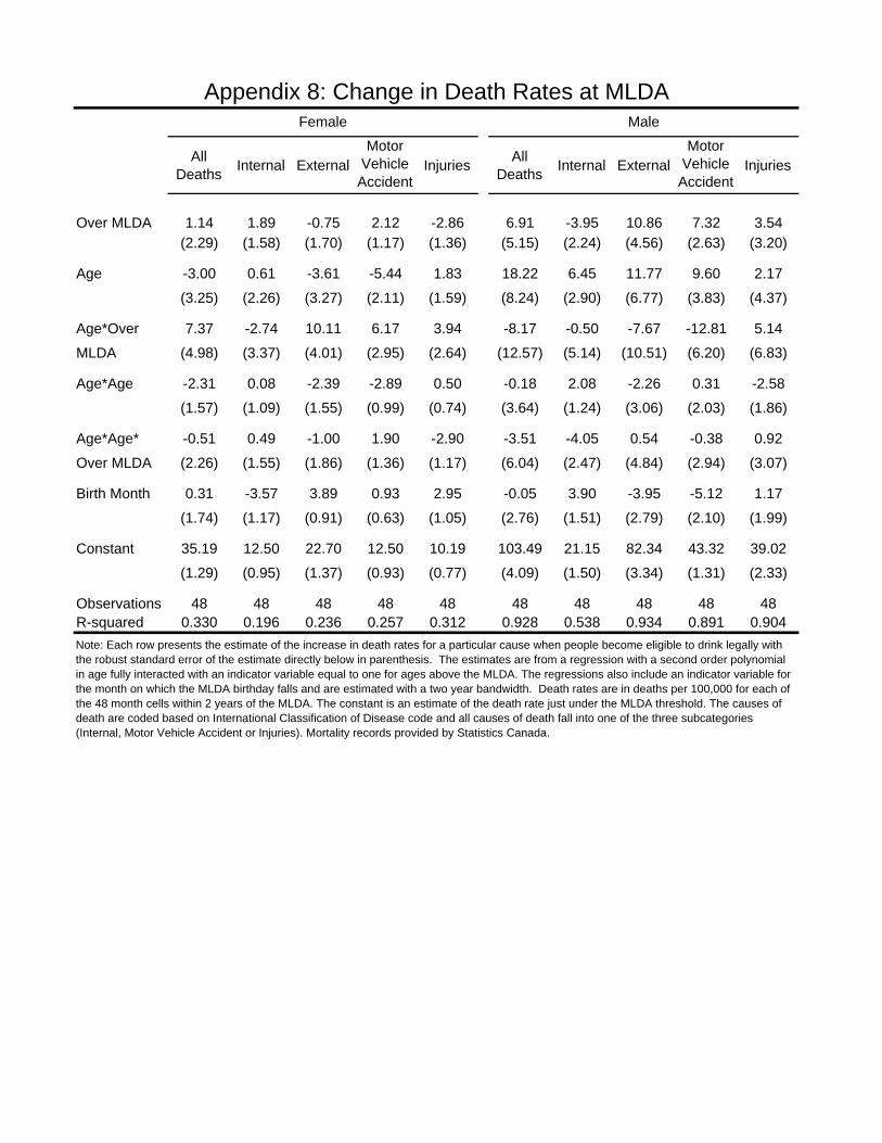
All Deaths
Internal ExternalMotor
Vehicle Accident
InjuriesAll
DeathsInternal External
Motor Vehicle
AccidentInjuries
Over MLDA 1.14 1.89 -0.75 2.12 -2.86 6.91 -3.95 10.86 7.32 3.54(2.29) (1.58) (1.70) (1.17) (1.36) (5.15) (2.24) (4.56) (2.63) (3.20)
Age -3.00 0.61 -3.61 -5.44 1.83 18.22 6.45 11.77 9.60 2.17
(3.25) (2.26) (3.27) (2.11) (1.59) (8.24) (2.90) (6.77) (3.83) (4.37)
Age*Over 7.37 -2.74 10.11 6.17 3.94 -8.17 -0.50 -7.67 -12.81 5.14
MLDA (4.98) (3.37) (4.01) (2.95) (2.64) (12.57) (5.14) (10.51) (6.20) (6.83)
Age*Age -2.31 0.08 -2.39 -2.89 0.50 -0.18 2.08 -2.26 0.31 -2.58
(1.57) (1.09) (1.55) (0.99) (0.74) (3.64) (1.24) (3.06) (2.03) (1.86)
Age*Age* -0.51 0.49 -1.00 1.90 -2.90 -3.51 -4.05 0.54 -0.38 0.92
Over MLDA (2.26) (1.55) (1.86) (1.36) (1.17) (6.04) (2.47) (4.84) (2.94) (3.07)
Birth Month 0.31 -3.57 3.89 0.93 2.95 -0.05 3.90 -3.95 -5.12 1.17
(1.74) (1.17) (0.91) (0.63) (1.05) (2.76) (1.51) (2.79) (2.10) (1.99)
Constant 35.19 12.50 22.70 12.50 10.19 103.49 21.15 82.34 43.32 39.02
(1.29) (0.95) (1.37) (0.93) (0.77) (4.09) (1.50) (3.34) (1.31) (2.33)
Observations 48 48 48 48 48 48 48 48 48 48R-squared 0.330 0.196 0.236 0.257 0.312 0.928 0.538 0.934 0.891 0.904
Female Male
Appendix 8: Change in Death Rates at MLDA
Note: Each row presents the estimate of the increase in death rates for a particular cause when people become eligible to drink legally with the robust standard error of the estimate directly below in parenthesis. The estimates are from a regression with a second order polynomial in age fully interacted with an indicator variable equal to one for ages above the MLDA. The regressions also include an indicator variable for the month on which the MLDA birthday falls and are estimated with a two year bandwidth. Death rates are in deaths per 100,000 for each of the 48 month cells within 2 years of the MLDA. The constant is an estimate of the death rate just under the MLDA threshold. The causes of death are coded based on International Classification of Disease code and all causes of death fall into one of the three subcategories (Internal, Motor Vehicle Accident or Injuries). Mortality records provided by Statistics Canada.

Drank Last 12 Months
Drank Last Week
Binged Last Week
Extreme Drinking
Last Week
Percent of Days Drank Last Week
Percent of Days
Binged Last Week
Percent of Days
Extreme Drinking
Last week
Max Drinks in One Day Last Week
Total Drinks in
Last Week
Over MLDA 2.92 7.96 4.96 2.65 3.54 1.76 0.51 0.48 1.16(1.658) (2.409) (1.836) (1.226) (0.885) (0.474) (0.260) (0.168) (0.335)
Week after 2.63 19.63 17.43 12.12 6.66 3.52 2.71 1.94 2.93Birthday (2.823) (4.684) (3.788) (4.183) (1.688) (1.058) (1.013) (0.539) (0.845)Age 1.47 2.35 0.92 0.22 0.50 0.07 0.03 9.76 9.48 (0.824) (0.973) (0.743) (0.407) (0.296) (0.184) (0.090) (6.392) (11.794)Age*Age -0.67 0.77 -0.32 -0.34 -0.07 -0.23 -0.09 -2.64 -12.53 (1.098) (1.294) (0.958) (0.508) (0.400) (0.238) (0.112) (8.087) (14.990)Age * Over -1.24 5.99 7.84 5.15 6.39 2.65 1.50 122.47 283.19MLDA (10.846) (15.644) (12.104) (7.964) (5.935) (3.105) (1.684) (111.915) (214.001)Age*Age -0.71 -3.93 -1.74 -0.47 -1.06 -0.24 -0.09 -22.34 -30.59*Over MLDA (1.446) (2.085) (1.615) (1.048) (0.803) (0.411) (0.221) (14.664) (27.981)Newfoundland -0.16 -0.29 5.74 2.09 -0.86 1.25 0.35 0.43 0.45
(1.316) (1.891) (1.622) (1.165) (0.793) (0.459) (0.253) (0.177) (0.323)PEI -0.97 -4.75 1.52 -0.55 -3.46 -0.21 -0.34 -0.02 -0.69
(1.629) (2.792) (2.658) (2.021) (1.029) (0.761) (0.423) (0.316) (0.505)Nova Scotia -2.90 -5.32 0.84 2.16 -3.44 0.05 0.26 0.00 -0.34
(1.499) (1.797) (1.710) (1.402) (0.607) (0.460) (0.307) (0.183) (0.354)New Brunswick 0.58 -4.74 -1.33 -1.95 -3.39 -0.99 -0.47 -0.35 -1.04
(1.300) (2.001) (1.719) (1.155) (0.665) (0.407) (0.263) (0.148) (0.307)Quebec 4.68 -0.36 -2.39 -3.11 -0.89 -0.95 -0.80 -0.40 -0.88
(0.779) (1.252) (1.003) (0.519) (0.467) (0.241) (0.115) (0.081) (0.161)
Manitoba -2.68 -6.57 -1.05 1.47 -2.62 -0.46 0.28 -0.05 -0.29(1.269) (1.532) (1.260) (0.945) (0.546) (0.314) (0.219) (0.140) (0.269)
Saskatchewan 4.91 6.81 7.86 4.70 1.97 1.68 0.99 0.82 1.26(1.044) (1.624) (1.472) (1.125) (0.690) (0.416) (0.294) (0.152) (0.331)
Alberta -1.81 -2.61 -2.15 -0.43 -1.43 -0.56 -0.07 -0.18 -0.41(0.917) (1.309) (1.037) (0.745) (0.495) (0.272) (0.162) (0.103) (0.192)
BC 1.25 -0.98 -0.80 -1.63 -1.20 -0.43 -0.31 -0.17 -0.45(0.986) (1.257) (1.024) (0.673) (0.475) (0.268) (0.158) (0.096) (0.200)
Territories 9.90 3.50 6.02 1.60 0.02 0.85 0.09 0.33 0.13(1.726) (2.791) (2.217) (1.554) (1.006) (0.557) (0.327) (0.217) (0.367)
1994 -2.04 -5.36 -1.99 -2.40 -2.12 -0.84 -0.55 -0.40 -0.81(2.256) (2.585) (2.092) (1.420) (0.951) (0.559) (0.293) (0.220) (0.423)
1995 -3.49 -8.35 -7.74 -3.21 -3.29 -1.88 -0.97 -0.68 -1.38(3.559) (3.919) (2.825) (1.657) (1.185) (0.650) (0.315) (0.247) (0.437)
1996 -2.20 -9.52 -7.05 -3.73 -3.39 -2.11 -0.95 -0.74 -1.52(1.984) (2.529) (1.890) (1.106) (0.856) (0.431) (0.223) (0.162) (0.296)
1997 -0.55 -13.32 -5.99 -4.20 -4.60 -1.70 -0.84 -0.72 -1.37(2.725) (3.017) (2.658) (0.949) (0.832) (0.514) (0.203) (0.201) (0.324)
1998 -3.17 -4.26 -2.35 -2.24 -1.39 -1.31 -0.73 -0.50 -1.12(2.263) (2.542) (2.206) (1.440) (1.008) (0.503) (0.268) (0.182) (0.324)
1999 0.51 -10.47 -6.88 -1.72 -3.62 -1.60 -0.04 -0.41 -0.63(3.354) (4.211) (3.210) (2.421) (1.628) (0.878) (0.647) (0.393) (0.842)
2000 1.22 -3.47 -0.89 -2.71 -1.18 -0.54 -0.64 -0.33 -0.65(1.497) (1.818) (1.476) (0.876) (0.665) (0.389) (0.206) (0.138) (0.273)
2001 -0.04 -3.58 -4.44 -2.93 -1.08 -1.16 -0.63 -0.51 -0.87(1.037) (1.298) (1.020) (0.664) (0.511) (0.277) (0.151) (0.098) (0.194)
2002 0.93 1.52 -0.79 -1.66 0.11 -0.21 -0.42 -0.19 -0.29(1.390) (1.696) (1.360) (0.901) (0.615) (0.374) (0.201) (0.124) (0.255)
2003 1.82 -0.26 -1.75 -0.90 0.01 -0.53 -0.21 -0.19 -0.29(1.009) (1.234) (0.954) (0.680) (0.509) (0.250) (0.155) (0.094) (0.190)
2004 0.95 -0.09 -1.02 -2.14 -0.71 -0.77 -0.58 -0.21 -0.62(1.318) (2.114) (1.606) (0.962) (0.689) (0.394) (0.209) (0.155) (0.271)
2008 0.48 0.64 -0.48 -1.28 0.78 -0.21 -0.12 -0.07 0.07(1.279) (1.840) (1.671) (1.126) (0.909) (0.525) (0.347) (0.182) (0.515)
2009 2.52 -1.29 -1.10 -1.49 -1.40 -0.41 -0.20 -0.12 -0.34
Appendix 9: Change in Drinking at MLDA (Full Model)

(1.131) (2.100) (1.710) (1.099) (0.713) (0.455) (0.290) (0.206) (0.375)2010 -1.35 -2.04 -3.65 -3.75 -2.70 -1.65 -0.96 -0.52 -1.37
(1.329) (2.142) (1.644) (1.042) (0.653) (0.363) (0.212) (0.156) (0.259)2011 -1.40 -3.71 -5.14 -3.53 -2.37 -1.26 -0.72 -0.56 -1.06
(1.388) (1.874) (1.435) (0.829) (0.631) (0.387) (0.212) (0.123) (0.259)January 0.42 -2.47 0.86 -0.65 0.02 0.24 -0.06 -0.11 -0.01
(1.543) (2.017) (1.726) (1.161) (0.761) (0.453) (0.272) (0.178) (0.350)February 2.04 -2.48 -1.23 -2.06 -0.51 -0.51 -0.55 -0.33 -0.57
(1.509) (1.880) (1.523) (1.049) (0.853) (0.374) (0.225) (0.154) (0.290)March 1.03 -4.63 -2.23 -2.86 -1.06 -0.65 -0.46 -0.43 -0.62
(1.540) (1.845) (1.462) (1.008) (0.673) (0.368) (0.239) (0.152) (0.293)May 1.11 -0.14 0.63 -1.26 0.18 0.07 -0.14 -0.16 -0.15
(1.376) (1.788) (1.474) (1.035) (0.654) (0.390) (0.255) (0.153) (0.298)June 1.89 1.08 0.35 -0.28 0.84 0.01 -0.12 0.02 0.01
(1.415) (1.816) (1.504) (1.062) (0.692) (0.380) (0.233) (0.163) (0.292)July 1.46 4.14 1.70 -0.70 2.54 0.58 -0.13 0.06 0.38
(1.362) (1.843) (1.544) (1.087) (0.728) (0.424) (0.255) (0.164) (0.316)August 2.32 1.02 -0.69 -2.50 1.26 -0.09 -0.26 -0.25 -0.10
(1.435) (1.841) (1.475) (0.960) (0.723) (0.388) (0.236) (0.150) (0.294)September 0.41 0.80 0.45 -1.52 1.14 0.26 -0.10 -0.05 0.24
(1.522) (1.793) (1.459) (0.991) (0.772) (0.427) (0.269) (0.161) (0.375)October 0.85 -2.31 -1.35 -2.12 -0.26 -0.29 -0.37 -0.31 -0.39
(1.440) (1.824) (1.479) (0.983) (0.704) (0.399) (0.232) (0.153) (0.297)November 0.51 -4.54 -2.14 -1.23 -0.99 -0.61 -0.18 -0.30 -0.43
(1.472) (1.907) (1.566) (1.138) (0.738) (0.394) (0.254) (0.175) (0.319)December 2.44 -0.04 -0.66 -2.61 -0.36 -0.31 -0.44 -0.28 -0.47
(1.702) (2.239) (1.805) (1.130) (0.773) (0.466) (0.275) (0.176) (0.336)Male 2.24 8.33 7.54 6.05 4.60 2.11 1.39 1.31 2.52
(0.596) (0.770) (0.627) (0.403) (0.291) (0.160) (0.091) (0.059) (0.116)White 22.49 21.15 13.87 5.30 6.91 3.14 1.15 1.33 2.35
(0.981) (1.111) (0.809) (0.444) (0.391) (0.193) (0.099) (0.073) (0.141)Married -2.53 -10.29 -9.80 -4.40 -4.56 -2.76 -1.15 -0.89 -1.89
(1.499) (2.291) (1.741) (1.089) (0.774) (0.420) (0.214) (0.147) (0.268)Live with parents -1.32 -2.42 -1.68 -1.08 -0.53 -0.40 -0.21 -0.12 -0.20
(0.801) (1.009) (0.815) (0.543) (0.367) (0.213) (0.126) (0.076) (0.149)Interview in person -3.00 -4.36 -2.01 -0.53 -1.29 -0.44 -0.13 -0.19 -0.33
(0.653) (0.840) (0.682) (0.440) (0.319) (0.182) (0.108) (0.066) (0.140)In school 0.65 -1.43 -2.66 -3.47 -1.80 -1.13 -0.87 -0.46 -1.11
(0.652) (0.945) (0.777) (0.509) (0.404) (0.212) (0.118) (0.076) (0.157)
Worked last week 6.34 5.12 2.78 0.65 0.87 0.24 -0.03 0.25 0.12(0.640) (0.790) (0.645) (0.381) (0.304) (0.168) (0.093) (0.058) (0.123)
Missing school 14.19 13.11 7.90 4.97 4.52 1.69 0.83 1.02 1.66 Information (8.906) (7.739) (5.007) (3.284) (2.762) (1.200) (0.636) (0.596) (1.018)
Missing work -2.41 -0.37 1.76 -0.89 -0.22 0.58 -0.07 -0.09 0.03 information (10.236) (6.933) (4.292) (2.520) (2.398) (1.003) (0.491) (0.494) (0.849)Constant 58.3 23.3 9.8 6.5 5.4 2.6 1.4 1.18 1.93
(2.3) (2.6) (2.0) (1.3) (0.9) (0.6) (0.3) (0.191) (0.399)
R-squared 0.108 0.107 0.068 0.049 0.111 0.059 0.043 0.098 0.086Mean 78.8 34.9 17 6.06 9.16 3.61 1.25 1.774 2.808Observations 44,694 36,389 36,389 36,389 36,389 36,389 36,389 36,389 36,389

Drank Last 12 Months
Drank Last
Week
Binged Last
Week
Extreme Drinking
Last Week
Percent of Days
Drank Last Week
Percent of Days
Binged Last Week
Percent of Days
Extreme Drinking
Last week
Max Drinks in One Day
Last Week
Total Drinks in
Last Week
Full set of Covariates Linear Controls Over MLDA 3.6 11.5 6.5 3.1 4.5 2.0 0.6 0.68 1.43
(1.1) (1.5) (1.2) (0.8) (0.5) (0.3) (0.2) (0.11) (0.23)
Week after 1.4 16.9 15.6 11.4 5.7 3.1 2.6 1.72 2.56 Birthday (2.7) (4.5) (3.6) (4.1) (1.6) (1) (1) (0.53) (0.82)
Full set of Covariates Quadratic Controls Over MLDA 2.9 8.0 5.0 2.7 3.5 1.8 0.5 0.48 1.16
(1.7) (2.4) (1.8) (1.2) (0.9) (0.5) (0.3) (0.17) (0.34)
Week after 2.6 19.6 17.4 12.1 6.7 3.5 2.7 1.94 2.93 Birthday (2.8) (4.7) (3.8) (4.2) (1.7) (1.1) (1) (0.54) (0.85)
Full set of Covariates Cubic Controls Over MLDA 3.2 13.7 6.8 5.2 6.0 2.1 1.0 0.90 1.88
(2.2) (3.1) (2.4) (1.6) (1.1) (0.6) (0.3) (0.21) (0.41)
Week after 3.2 16.3 16.2 10.1 4.9 3.3 2.3 1.64 2.39 Birthday (3) (4.9) (4) (4.3) (1.8) (1.1) (1) (0.55) (0.86)
Observations 44,694 36,389 36,389 36,389 36,389 36,389 36,389 36,389 36,389
Appendix 10: Change in Drinking at MLDA
Note: See notes for Table 3 for a description of the sample. All regressions include a first, second or third order polynomial in age fully interacted with an indicator variable that takes on a value of 1 for people interviewed when they are older than the MLDA. The estimates in the top row of each panel in the table are for the coefficients on this indicator variable with its standard error directly below in parenthesis. The regressions also include an indicator variable that takes on a value of one if the person is interviewed in the week immediately after the birthday on which they become eligible to drink legally. This is intended to absorb the pronounced "celebration" effects noticeable in the age profiles and is presented in the second major row of each panel. For the binary outcome variables the point estimates and their SE have been multiplied by 100 to make them easier to read and interpretable as percentage points. The standard errors are clustered on the running variable. The regressions are weighted to account for the sampling frame. Extreme drinking is 8 or more drinks in a day for women and 10 or more drinks in a day for men. All the regressions also include controls for year of survey, province of residence, white, marital status, living with parents, interview in person, in school, work last week, gender, month of interview, and dummies flagging when in school or work last week are missing. The means on the second to last row are for the subsample of people interviewed when they are within one year of reaching the provincial MLDA.
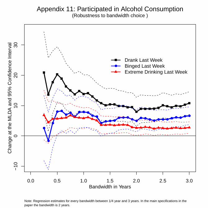
●
●
●
● ●
●●
●
● ● ●● ●
●● ● ●
● ● ●●
●● ● ● ● ● ● ● ● ● ● ● ●
0.0 0.5 1.0 1.5 2.0 2.5 3.0Bandwidth in Years
−10
010
2030
Cha
nge
at th
e M
LDA
and
95%
Con
fiden
ce In
terv
al
●
Drank Last WeekBinged Last WeekExtreme Drinking Last Week
Appendix 11: Participated in Alcohol Consumption(Robustness to bandwidth choice )
Note: Regression estimates for every bandwidth between 1/4 year and 3 years. In the main specifications in the paper the bandwidth is 2 years.

●
●
●
● ● ● ●●
● ● ●● ●
● ● ● ●● ● ● ● ●
● ● ● ● ● ● ● ● ● ● ● ●
0.0 0.5 1.0 1.5 2.0 2.5 3.0Bandwidth in Years
05
1015
Cha
nge
at th
e M
LDA
and
95%
Con
fiden
ce In
terv
al
●
DrinkingBinge DrinkingExtreme Drinking
Appendix 12: Percent of Days Drinking Last Week(Robustness to bandwidth choice )
Note: Regression estimates for every bandwidth between 1/4 year and 3 years. In the main specifications in the paper the bandwidth is 2 years.

●
●
● ● ● ● ● ●● ● ● ● ● ● ● ● ● ● ● ● ● ● ● ● ● ● ● ● ● ● ● ● ● ●
0.0 0.5 1.0 1.5 2.0 2.5 3.0Bandwidth in Years
−10
−5
05
10C
hang
e at
the
MLD
A a
nd 9
5% C
onfid
ence
Inte
rval
●
Drank Last 12 MonthsTotal Drinks in WeekMaximum Drinks in Day
Appendix 13: Drank Last 12 Months, Maximum and Total Drinks(Robustness to bandwidth choice )
Note: Regression estimates for every bandwidth between 1/4 year and 3 years. In the main specifications in the paper the bandwidth is 2 years.
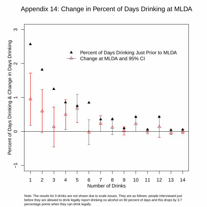
1 2 3 4 5 6 7 8 9 10 11 12 13 14Number of Drinks
−1
01
23
Per
cent
of D
ays
Drin
king
& C
hang
e in
Day
s D
rinki
ngAppendix 14: Change in Percent of Days Drinking at MLDA
Percent of Days Drinking Just Prior to MLDAChange at MLDA and 95% CI
Note: The results for 0 drinks are not shown due to scale issues. They are as follows: people interviewed just before they are allowed to drink legally report drinking no alcohol on 90 percent of days and this drops by 3.7 percentage points when they can drink legally.
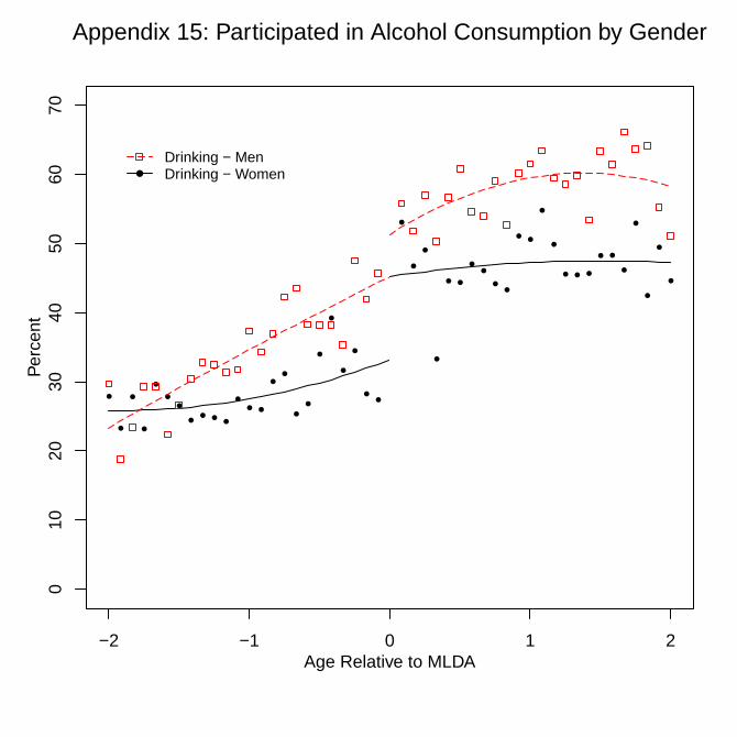
●
●
●
●
●
●
●
●● ●
●
●
● ●
●●
●
●
●
●
●
●
●●
●
●
●
●
● ●
●●
●●
●●
●
●
● ● ●
● ●
●
●
●
●
●
−2 −1 0 1 2Age Relative to MLDA
010
2030
4050
6070
Per
cent
●
Drinking − MenDrinking − Women
Appendix 15: Participated in Alcohol Consumption by Gender

●
●
● ●
●
● ●
●
●
●
●●
●
●●
●
● ●
●●
●
●
●
●
●●
●
●
●
●
●
● ●
●
●
●
●
●
●
●
● ●
●●
●
● ●●
−2 −1 0 1 2Age Relative to MLDA
010
2030
40P
erce
nt
●
MenWomen
Appendix 16: Participated in Binge Drinking by Gender
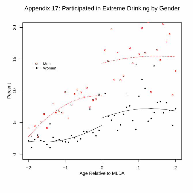
●
●
●
●
●●
●
●
●
●●
● ● ●
●
●
●
●
● ●
●
●
●
●
●
●
●
●
●
●
●
●●
●
●
●
●
●
●
●
●
● ●
●
●
●
●
●
−2 −1 0 1 2Age Relative to MLDA
05
1015
20P
erce
nt
●
MenWomen
Appendix 17: Participated in Extreme Drinking by Gender
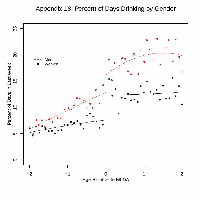
●
●
●
●
●●
● ●
●
● ●
● ●
●●
●
●
●
●●
●
●
●
●
●
●
●
●
● ●
●
● ●
●
●
●
●
●
●
●
●
●
● ●
●
●
●
●
−2 −1 0 1 2Age Relative to MLDA
05
1015
2025
Per
cent
of D
ays
in L
ast W
eek ●
MenWomen
Appendix 18: Percent of Days Drinking by Gender

●
●
● ●
●
●
●
●
● ●
● ●
●
●
●●
● ●
●● ●
●
●
●
●
●
●
●
● ●
●
●
●
●
●
●
●
●
●●
●
●
●
●
●
●
●
●
−2 −1 0 1 2Age Relative to MLDA
02
46
810
Per
cent
of D
ays
in L
ast W
eek ●
MenWomen
Appendix 19: Percent of Days Binge Drinking by Gender

●
●
●
●
●● ●
●
●●
● ● ●
●●
●
●●
●●
●
●
●
●
●
● ●●
●●
●
●
●●
●
●
●
●
●
●●
●
●
●
●
●
●
●
−2 −1 0 1 2Age Relative to MLDA
01
23
45
Per
cent
of D
ays
in L
ast W
eek ●
MenWomen
Appendix 20: Percent of Days Extreme Drinking by Gender
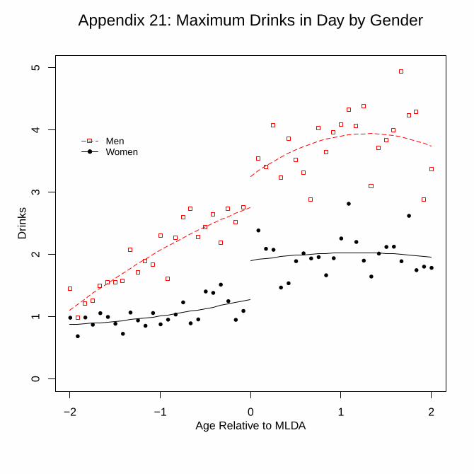
●
●
●
●
●●
●
●
●
●●
●
●●
●
●
●●
● ●
●
●
●
●
●
● ●
●●
●
●● ●
●
●
●
●
●
●
●
●
● ●
●
●
●● ●
−2 −1 0 1 2Age Relative to MLDA
01
23
45
Drin
ks
●
MenWomen
Appendix 21: Maximum Drinks in Day by Gender

●
●
●
●
● ●
●
●
●●
●
●
●
●●
●
●●
● ●
●
●
●
●
●
●
●
●
●
●
●
●
●●
●
●
●
●
● ●
●
●
● ●
●
●●
●
−2 −1 0 1 2Age Relative to MLDA
02
46
8D
rinks
●
MenWomen
Appendix 22: Total Drinks in Week by Gender

Drank Last 12 Months
Drank Last Week
Binged Last Week
Extreme Drinking
Last Week
Percent of Days Drank Last Week
Percent of Days
Binged Last Week
Percent of Days
Extreme Drinking
Last week
Max Drinks in One Day Last Week
Total Drinks in Last Week
Over MLDA 3.19 6.78 2.58 5.11 3.32 1.82 1.00 0.54 1.42
(2.279) (3.384) (2.659) (1.944) (1.337) (0.727) (0.433) (0.274) (0.552)
Week after 4.43 6.66 7.00 7.88 3.16 0.94 1.47 1.27 1.68
Birthday (5.112) (5.529) (6.832) (5.257) (2.432) (2.081) (1.223) (0.770) (1.432)
Age 2.02 2.73 1.82 -0.18 0.83 0.14 -0.07 14.39 13.58
(1.168) (1.337) (1.069) (0.660) (0.477) (0.287) (0.161) (10.453) (20.384)
Age*Age -0.10 -0.06 -0.13 -1.27 -0.02 -0.34 -0.31 -7.63 -24.40
(1.558) (1.742) (1.357) (0.842) (0.639) (0.368) (0.201) (13.069) (25.694)
Age * Over -6.10 8.02 1.06 3.60 8.81 1.55 1.55 113.89 360.57
MLDA (15.276) (21.596) (17.329) (12.664) (9.174) (4.672) (2.778) (181.494) (350.887)
Age*Age -1.74 -3.86 -1.92 1.08 -1.74 -0.06 0.24 -21.55 -31.57
*Over MLDA (2.037) (2.842) (2.358) (1.694) (1.237) (0.627) (0.369) (24.036) (46.271)
Newfoundland -0.73 0.68 8.27 4.55 -0.82 2.06 0.74 0.73 0.76
(1.804) (2.745) (2.663) (2.129) (1.336) (0.794) (0.462) (0.315) (0.565)
PEI -3.85 -6.71 -1.18 -3.27 -5.24 -0.96 -1.35 -0.48 -1.83
(2.231) (3.899) (3.985) (3.019) (1.705) (1.279) (0.473) (0.432) (0.749)
Nova Scotia -1.93 -4.87 3.06 5.00 -3.79 0.89 0.84 0.28 0.05
(1.782) (2.788) (2.807) (2.446) (1.064) (0.832) (0.574) (0.337) (0.671)
New Brunswick -1.97 -2.89 0.46 -2.12 -3.61 -1.01 -0.57 -0.39 -1.36
(2.006) (2.913) (2.675) (1.876) (1.117) (0.648) (0.467) (0.256) (0.564)
Quebec 3.42 -2.79 -3.59 -5.16 -2.28 -1.47 -1.37 -0.74 -1.66
(1.129) (1.663) (1.327) (0.868) (0.740) (0.358) (0.201) (0.131) (0.272)
Manitoba -4.03 -8.98 -2.07 1.36 -3.47 -0.52 0.35 -0.12 -0.39
(1.812) (2.204) (1.909) (1.532) (0.921) (0.524) (0.395) (0.244) (0.495)
Saskatchewan 4.51 4.11 8.48 4.67 0.79 1.84 1.18 0.86 1.33
(1.426) (2.312) (2.201) (1.803) (1.030) (0.659) (0.510) (0.249) (0.562)
Alberta -2.53 -3.39 -4.10 -1.27 -2.27 -0.85 -0.22 -0.32 -0.70
(1.251) (1.884) (1.537) (1.250) (0.793) (0.424) (0.281) (0.177) (0.334)
BC -0.15 -2.35 -1.15 -2.53 -2.02 -0.51 -0.51 -0.30 -0.78
(1.351) (1.732) (1.547) (1.137) (0.786) (0.431) (0.278) (0.164) (0.344)
Territories 7.25 -5.71 2.18 0.80 -3.95 -0.01 -0.16 -0.12 -0.84
(2.307) (4.040) (3.293) (2.511) (1.524) (0.862) (0.565) (0.377) (0.645)
1994 -2.86 -9.12 -2.38 -3.17 -3.21 -1.46 -0.91 -0.62 -1.40
(3.169) (3.627) (3.348) (2.479) (1.504) (0.892) (0.494) (0.389) (0.740)
1995 -1.65 -4.20 -7.78 -2.56 -2.58 -2.00 -1.20 -0.68 -1.64
(4.564) (5.992) (4.927) (3.274) (2.164) (1.259) (0.626) (0.493) (0.893)
1996 -4.05 -15.16 -12.03 -6.62 -5.10 -3.54 -1.65 -1.32 -2.65
(2.631) (3.503) (2.697) (1.779) (1.380) (0.667) (0.405) (0.274) (0.529)
1997 -5.08 -18.00 -9.12 -5.25 -6.47 -2.24 -1.11 -1.11 -2.06
(4.488) (3.408) (2.730) (1.625) (1.127) (0.681) (0.360) (0.279) (0.508)
1998 -5.15 -4.14 0.57 -1.62 -0.77 -0.86 -0.84 -0.48 -1.19
(3.183) (3.664) (3.411) (2.444) (1.600) (0.834) (0.460) (0.312) (0.571)
1999 1.00 -7.38 -3.82 2.45 -2.77 -0.27 1.07 0.18 0.56
(4.003) (6.625) (6.010) (5.399) (3.315) (1.958) (1.527) (0.879) (1.980)
2000 -0.99 -7.88 -3.59 -4.38 -2.73 -1.20 -0.99 -0.62 -1.21
(2.264) (2.674) (2.190) (1.370) (1.111) (0.646) (0.354) (0.244) (0.500)
2001 -0.33 -5.99 -5.58 -4.06 -1.66 -1.54 -0.90 -0.79 -1.33
(1.502) (1.807) (1.534) (1.081) (0.814) (0.437) (0.264) (0.161) (0.337)
2002 1.01 -1.83 -1.41 -2.83 -0.63 -0.48 -0.64 -0.38 -0.58
(1.839) (2.354) (2.064) (1.404) (0.968) (0.562) (0.338) (0.209) (0.432)
2003 2.05 -1.91 -2.39 -1.25 0.02 -0.86 -0.37 -0.31 -0.51
(1.353) (1.690) (1.451) (1.114) (0.849) (0.394) (0.267) (0.157) (0.326)
Appendix 23: Change in Drinking at MLDA - Males

2004 0.08 -5.55 -3.72 -4.09 -2.51 -1.66 -1.14 -0.63 -1.49
(1.810) (3.069) (2.533) (1.546) (1.110) (0.600) (0.352) (0.253) (0.455)
2008 0.11 -1.19 -1.53 -0.77 1.17 -0.21 -0.03 -0.11 0.19
(1.770) (2.617) (2.473) (1.905) (1.527) (0.905) (0.621) (0.314) (0.938)
2009 2.31 -0.47 -0.83 -2.20 -1.97 -0.42 -0.47 -0.07 -0.49
(1.666) (2.954) (2.610) (1.832) (1.051) (0.733) (0.483) (0.371) (0.662)
2010 -3.82 -3.86 -5.06 -4.12 -4.38 -2.20 -1.36 -0.74 -2.12
(1.921) (2.960) (2.479) (1.862) (0.956) (0.574) (0.355) (0.281) (0.451)
2011 -2.06 -5.64 -8.82 -5.11 -3.61 -1.92 -1.04 -0.94 -1.74
(1.918) (2.604) (2.028) (1.397) (0.962) (0.652) (0.391) (0.210) (0.468)
January -0.23 -5.40 -2.13 -1.36 -0.23 -0.22 0.05 -0.28 -0.09
(2.197) (2.885) (2.468) (1.838) (1.202) (0.692) (0.470) (0.294) (0.616)
February 0.79 -5.71 -2.92 -2.32 -0.99 -1.06 -0.64 -0.45 -0.86
(2.182) (2.619) (2.351) (1.800) (1.518) (0.610) (0.401) (0.268) (0.531)
March 0.86 -4.55 -2.91 -3.36 -1.12 -0.81 -0.45 -0.51 -0.76
(2.252) (2.745) (2.269) (1.711) (1.108) (0.622) (0.431) (0.264) (0.537)
May -0.11 -0.60 -0.40 -1.05 0.45 -0.14 0.07 -0.18 -0.08
(2.012) (2.528) (2.263) (1.700) (1.060) (0.624) (0.448) (0.271) (0.543)
June 3.08 2.51 2.17 0.69 1.38 0.34 0.04 0.23 0.26
(2.028) (2.546) (2.267) (1.709) (1.097) (0.613) (0.393) (0.280) (0.519)
July 2.21 1.29 0.42 -0.17 2.62 0.53 -0.03 0.01 0.45
(1.960) (2.653) (2.328) (1.782) (1.161) (0.656) (0.415) (0.271) (0.524)
August 2.74 -0.52 -0.97 -2.65 1.39 -0.07 -0.08 -0.27 0.02
(2.040) (2.656) (2.351) (1.618) (1.159) (0.625) (0.414) (0.262) (0.524)
September 0.16 1.09 0.81 -1.32 1.83 0.42 0.03 0.02 0.52
(2.183) (2.644) (2.256) (1.618) (1.314) (0.709) (0.469) (0.283) (0.687)
October 0.73 -3.49 -2.40 -2.35 -0.35 -0.43 -0.40 -0.42 -0.52
(2.068) (2.627) (2.248) (1.603) (1.130) (0.647) (0.394) (0.265) (0.525)
November 1.75 -4.58 -2.34 -0.52 -0.31 -0.59 0.01 -0.26 -0.31
(2.117) (2.722) (2.418) (1.857) (1.190) (0.633) (0.426) (0.306) (0.563)
December 0.64 -3.05 -1.19 -3.21 -0.79 -0.50 -0.50 -0.44 -0.75
(2.476) (3.289) (2.800) (1.857) (1.260) (0.764) (0.482) (0.308) (0.599)
White 21.24 25.23 17.58 8.16 8.91 4.24 1.82 1.86 3.43(1.363) (1.504) (1.007) (0.722) (0.631) (0.276) (0.170) (0.118) (0.239)
Married -0.45 -9.56 -10.18 -3.83 -5.35 -3.17 -1.26 -1.02 -2.45
(2.685) (4.532) (3.647) (2.676) (1.597) (0.860) (0.525) (0.359) (0.612)
Live with parents 0.12 -1.78 -1.07 -1.05 -0.61 -0.41 -0.20 -0.13 -0.29
(1.122) (1.465) (1.231) (0.902) (0.603) (0.343) (0.217) (0.132) (0.266)
Interview in perso -3.46 -2.74 -1.28 -0.63 -1.20 -0.39 -0.23 -0.14 -0.34
(0.935) (1.197) (1.029) (0.743) (0.494) (0.287) (0.188) (0.112) (0.239)
In school -0.21 -2.76 -2.51 -3.98 -2.65 -1.27 -1.11 -0.56 -1.46
(0.916) (1.290) (1.097) (0.800) (0.624) (0.309) (0.195) (0.122) (0.258)
Worked last week 4.22 3.84 2.63 0.55 0.21 0.00 -0.18 0.21 -0.13
(0.906) (1.134) (0.936) (0.644) (0.507) (0.265) (0.167) (0.098) (0.217)
Missing school 22.94 20.40 14.19 7.51 6.43 2.90 1.36 1.61 2.50
Information (10.524) (10.606) (7.282) (5.066) (4.105) (1.831) (1.004) (0.927) (1.620)
Missing work -11.71 -4.42 0.86 1.34 0.13 0.66 0.19 -0.01 0.43
information (12.448) (7.876) (4.946) (3.309) (3.156) (1.228) (0.642) (0.635) (1.135)
Constant 64.3 34.5 18.1 11.2 10.6 4.8 2.6 2.52 4.55
(3.2) (3.7) (3.1) (2.1) (1.5) (0.9) (0.6) (0.327) (0.703)
R-squared 0.108 0.129 0.075 0.048 0.120 0.060 0.041 0.088 0.076
Mean 79.2 39.8 21.7 8.89 11.1 4.77 1.9 2.411 3.916Observations 22,139 17,894 17,894 17,894 17,894 17,894 17,894 17,894 17,894

Drank Last 12 Months
Drank Last Week
Binged Last Week
Extreme Drinking
Last Week
Percent of Days Drank Last Week
Percent of Days
Binged Last Week
Percent of Days
Extreme Drinking
Last week
Max Drinks in One Day Last Week
Total Drinks in Last Week
Over MLDA 2.14 8.43 7.06 -0.06 3.55 1.63 -0.03 0.37 0.80
(2.471) (3.291) (2.479) (1.374) (0.991) (0.556) (0.257) (0.176) (0.306)
Week after 0.90 33.18 27.92 16.44 10.16 6.10 3.92 2.63 4.18
Birthday (2.764) (9.071) (9.398) (5.309) (3.158) (2.200) (1.611) (0.778) (1.395)
Age -1.30 1.90 -0.20 0.72 -0.02 -0.04 0.14 8.16 10.10
(1.644) (1.863) (1.269) (0.556) (0.472) (0.261) (0.098) (6.557) (10.046)
Age*Age 5.58 1.94 11.63 6.24 3.09 3.16 1.43 5.58 4.01
(15.802) (21.120) (16.361) (8.498) (6.314) (3.691) (1.678) (8.471) (13.254)
Age * Over 0.11 -4.55 -1.88 -2.29 -0.54 -0.50 -0.47 106.19 166.04
MLDA (2.134) (2.833) (2.175) (1.123) (0.857) (0.490) (0.223) (112.142) (195.994)
Age*Age 0.93 2.29 0.29 0.73 0.28 0.06 0.14 -27.91 -36.50
*Over MLDA (1.217) (1.390) (0.954) (0.459) (0.344) (0.195) (0.080) (14.905) (26.028)
Newfoundland 0.36 -1.43 3.30 -0.20 -0.97 0.46 -0.04 0.14 0.13
(1.961) (2.400) (1.903) (1.123) (0.776) (0.480) (0.244) (0.170) (0.323)
PEI 1.74 -3.16 4.10 1.97 -1.77 0.51 0.60 0.39 0.36
(2.388) (4.149) (3.481) (2.641) (1.175) (0.836) (0.671) (0.439) (0.653)
Nova Scotia -3.80 -5.33 -1.15 -0.36 -2.88 -0.70 -0.25 -0.22 -0.63
(2.446) (2.477) (2.036) (1.132) (0.610) (0.398) (0.177) (0.135) (0.198)
New Brunswick 3.22 -6.94 -3.37 -1.89 -3.18 -1.03 -0.39 -0.33 -0.74
(1.644) (2.787) (2.228) (1.321) (0.708) (0.489) (0.234) (0.154) (0.241)
Quebec 5.91 1.96 -1.33 -1.25 0.40 -0.47 -0.28 -0.09 -0.16
(1.072) (1.772) (1.431) (0.617) (0.517) (0.314) (0.115) (0.089) (0.153)
Manitoba -1.33 -4.06 0.05 1.75 -1.66 -0.37 0.26 0.05 -0.12
(1.802) (2.084) (1.652) (1.129) (0.558) (0.356) (0.192) (0.130) (0.196)
Saskatchewan 5.43 9.14 6.64 4.45 3.09 1.39 0.73 0.71 1.09
(1.540) (2.279) (1.890) (1.294) (0.869) (0.465) (0.255) (0.166) (0.299)
Alberta -0.98 -1.52 0.01 0.66 -0.41 -0.19 0.13 -0.01 -0.04
(1.343) (1.831) (1.423) (0.824) (0.567) (0.341) (0.157) (0.103) (0.182)
BC 2.60 0.28 -0.65 -0.90 -0.44 -0.39 -0.15 -0.08 -0.16
(1.406) (1.764) (1.348) (0.720) (0.509) (0.313) (0.149) (0.099) (0.192)
Territories 12.61 11.94 9.02 1.88 3.53 1.47 0.22 0.66 0.84
(2.619) (3.804) (3.008) (1.836) (1.293) (0.716) (0.312) (0.221) (0.363)
1994 -1.43 -1.23 -1.51 -1.39 -0.87 -0.11 -0.12 -0.15 -0.12
(3.152) (3.660) (2.434) (1.391) (1.117) (0.718) (0.349) (0.182) (0.398)
1995 -5.54 -11.38 -7.40 -3.66 -3.83 -1.69 -0.74 -0.65 -1.11
(5.038) (4.862) (3.362) (1.144) (1.213) (0.607) (0.200) (0.190) (0.298)
1996 -0.26 -3.73 -1.95 -0.87 -1.66 -0.69 -0.26 -0.16 -0.40
(2.822) (3.648) (2.568) (1.281) (1.050) (0.551) (0.201) (0.173) (0.281)
1997 3.36 -9.13 -3.14 -3.33 -2.97 -1.21 -0.62 -0.37 -0.77
(2.774) (4.430) (4.140) (0.905) (1.005) (0.680) (0.160) (0.253) (0.319)
1998 -1.04 -4.00 -5.70 -2.85 -1.84 -1.82 -0.61 -0.51 -0.98
(3.103) (3.451) (2.652) (1.292) (1.156) (0.510) (0.244) (0.158) (0.253)
1999 0.24 -12.45 -9.05 -4.49 -4.18 -2.52 -0.77 -0.79 -1.40
(4.953) (5.047) (3.389) (1.507) (1.383) (0.585) (0.245) (0.228) (0.330)
2000 3.15 1.46 2.24 -0.90 0.47 0.21 -0.26 0.01 -0.04
(1.919) (2.473) (2.004) (1.055) (0.745) (0.450) (0.200) (0.131) (0.226)
2001 0.19 -0.77 -3.04 -1.62 -0.35 -0.70 -0.31 -0.20 -0.33
(1.443) (1.771) (1.359) (0.736) (0.579) (0.338) (0.144) (0.104) (0.179)
2002 0.57 5.26 -0.09 -0.23 0.99 0.11 -0.15 0.04 0.07
(2.068) (2.326) (1.759) (1.165) (0.724) (0.490) (0.212) (0.133) (0.250)
2003 1.51 1.75 -0.86 -0.44 0.10 -0.14 -0.03 -0.03 -0.02
(1.462) (1.677) (1.253) (0.746) (0.507) (0.320) (0.150) (0.095) (0.184)
Appendix 24: Change in Drinking at MLDA - Females

2004 1.77 5.00 1.42 -0.38 0.90 0.02 -0.09 0.17 0.14
(1.848) (2.729) (1.997) (1.112) (0.758) (0.484) (0.214) (0.170) (0.266)
2008 0.62 2.28 0.36 -2.09 0.19 -0.32 -0.28 -0.07 -0.16
(1.905) (2.455) (2.119) (0.945) (0.745) (0.425) (0.219) (0.133) (0.220)
2009 2.56 -2.33 -1.65 -0.78 -0.77 -0.45 0.07 -0.18 -0.18
(1.550) (2.914) (2.117) (1.216) (0.941) (0.525) (0.325) (0.160) (0.324)
2010 1.31 -0.08 -2.31 -3.27 -1.08 -1.11 -0.57 -0.31 -0.65
(1.845) (2.962) (2.112) (0.898) (0.824) (0.438) (0.218) (0.128) (0.225)
2011 -0.89 -1.70 -1.40 -1.99 -1.23 -0.63 -0.42 -0.19 -0.44
(2.003) (2.604) (1.983) (0.877) (0.763) (0.428) (0.165) (0.128) (0.221)
January 1.19 0.75 3.86 0.17 0.48 0.70 -0.14 0.09 0.16
(2.150) (2.718) (2.306) (1.398) (0.870) (0.575) (0.261) (0.191) (0.316)
February 3.33 0.58 0.21 -1.79 -0.03 -0.04 -0.44 -0.20 -0.27
(1.987) (2.577) (1.970) (1.126) (0.744) (0.461) (0.222) (0.161) (0.253)
March 1.38 -4.42 -1.49 -2.21 -0.88 -0.46 -0.43 -0.33 -0.43
(2.047) (2.359) (1.750) (1.041) (0.715) (0.414) (0.220) (0.148) (0.243)
May 2.60 0.74 1.76 -1.32 0.09 0.30 -0.32 -0.11 -0.14
(1.868) (2.515) (1.901) (1.122) (0.737) (0.472) (0.229) (0.152) (0.255)
June 0.95 0.09 -1.46 -1.20 0.58 -0.31 -0.26 -0.17 -0.15
(1.932) (2.527) (1.900) (1.264) (0.794) (0.445) (0.249) (0.166) (0.263)
July 0.85 7.71 3.27 -1.04 2.78 0.71 -0.15 0.17 0.44
(1.854) (2.444) (1.883) (1.145) (0.791) (0.497) (0.261) (0.168) (0.312)
August 2.10 2.96 -0.32 -2.25 1.36 -0.09 -0.39 -0.19 -0.13
(2.025) (2.591) (1.790) (1.040) (0.800) (0.454) (0.219) (0.145) (0.251)
September 0.85 0.86 0.24 -1.56 0.65 0.13 -0.21 -0.10 0.02
(2.088) (2.421) (1.793) (1.121) (0.769) (0.457) (0.251) (0.149) (0.263)
October 0.84 -1.09 -0.26 -1.84 -0.06 -0.15 -0.33 -0.18 -0.20
(2.016) (2.466) (1.827) (1.087) (0.757) (0.453) (0.232) (0.146) (0.253)
November -0.56 -4.15 -1.78 -1.78 -1.51 -0.59 -0.31 -0.30 -0.47
(2.108) (2.568) (1.912) (1.262) (0.764) (0.445) (0.267) (0.158) (0.264)
December 4.33 2.71 -0.57 -2.26 0.03 -0.24 -0.44 -0.18 -0.26
(2.227) (3.025) (2.146) (1.167) (0.826) (0.494) (0.239) (0.165) (0.277)
White 23.89 17.02 10.02 2.29 4.90 2.00 0.45 0.79 1.24(1.397) (1.505) (1.148) (0.510) (0.400) (0.252) (0.096) (0.073) (0.126)
Married -3.58 -9.62 -9.37 -4.10 -3.49 -2.39 -0.94 -0.70 -1.31
(1.811) (2.551) (1.945) (1.057) (0.826) (0.459) (0.196) (0.141) (0.256)
Live with parents -2.79 -3.43 -2.50 -1.36 -0.72 -0.49 -0.28 -0.17 -0.24
(1.050) (1.367) (1.044) (0.581) (0.405) (0.243) (0.122) (0.075) (0.136)
Interview in perso -2.51 -6.10 -2.82 -0.53 -1.42 -0.53 -0.05 -0.25 -0.34
(0.914) (1.104) (0.833) (0.437) (0.356) (0.206) (0.098) (0.061) (0.120)
In school 1.36 0.40 -2.57 -2.64 -0.56 -0.90 -0.55 -0.28 -0.59
(0.953) (1.233) (1.024) (0.611) (0.429) (0.277) (0.121) (0.079) (0.154)
Worked last week 8.41 6.03 2.73 0.61 1.31 0.41 0.08 0.26 0.29
(0.894) (1.113) (0.852) (0.398) (0.328) (0.196) (0.082) (0.058) (0.110)
Missing school -5.55 -4.19 -5.73 0.76 1.16 -0.99 -0.19 -0.18 -0.04
Information (7.739) (7.931) (6.455) (4.345) (3.143) (1.424) (0.800) (0.531) (0.919)
Missing work 18.58 15.65 10.23 -1.37 1.24 2.07 0.26 0.53 0.64
information (7.460) (8.401) (6.896) (4.093) (2.934) (1.553) (0.835) (0.527) (0.918)
Constant 54.6 20.6 9.7 8.1 4.8 2.6 1.6 1.19 1.86
(3.0) (3.4) (2.6) (1.5) (1.0) (0.6) (0.3) (0.191) (0.339)
R-squared 0.113 0.082 0.049 0.026 0.076 0.041 0.024 0.061 0.052
Mean 78.3 30 12.1 3.17 7.2 2.42 0.592 1.124 1.678Observations 22,555 18,495 18,495 18,495 18,495 18,495 18,495 18,495 18,495

−.2
−.1
0.1
.2.3
RD
Est
imat
es a
nd C
I
.5.6
.7.8
.91
Pro
port
ion
with
BA
C a
t or
Bel
ow th
is L
evel
0 .05 .1 .15 .2 .25 .3Blood Alcohol Concentration
Women Under MLDA Women Over MLDA
Men Under MLDA Men Over MLDA
RD Estimate and 95% CI − Women RD Estimate and 95% CI − Men
Appendix 25: Drinks Evenly Spaced Over 4 Hours

1 2 3 4 5 6 7 8 9 10 11 12 13 14Number of Drinks
−1
01
23
Per
cent
of D
ays
Drin
king
& C
hang
e in
Day
s D
rinki
ng
●
● ● ●
●
●
●
●●
● ●● ● ●
●
●
●
● ● ●
● ●
●
●
●●
● ●
Appendix 26: Change in Percent of Days Drinking at MLDA
● Female − Change at MLDA and 95% CIMale − Change at MLDA and 95% CI
● Female − Percent of Days Drinking Just Prior to MLDAMale − Percent of Days Drinking Just Prior to MLDA
Note: The results for 0 drinks are not shown due to scale issues. They are as follows: women interviewed just before they are allowed to drink legally report drinking no alcohol on 92 percent of days and this drops by 3.9 percentage points when they can drink legally. For men the corresponding numbers are 92 percent and 3.5 percentage point decline.
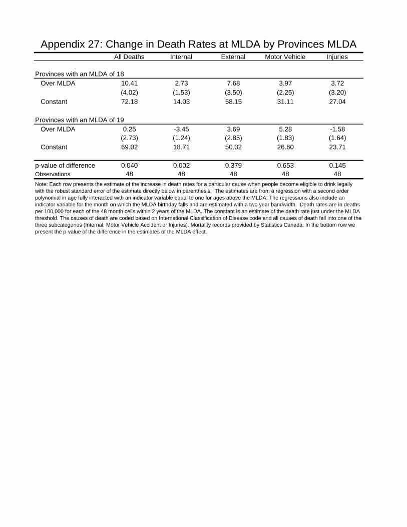
All Deaths Internal External Motor Vehicle Injuries
Provinces with an MLDA of 18 Over MLDA 10.41 2.73 7.68 3.97 3.72
(4.02) (1.53) (3.50) (2.25) (3.20) Constant 72.18 14.03 58.15 31.11 27.04
Provinces with an MLDA of 19 Over MLDA 0.25 -3.45 3.69 5.28 -1.58
(2.73) (1.24) (2.85) (1.83) (1.64) Constant 69.02 18.71 50.32 26.60 23.71
p-value of difference 0.040 0.002 0.379 0.653 0.145Observations 48 48 48 48 48
Appendix 27: Change in Death Rates at MLDA by Provinces MLDA
Note: Each row presents the estimate of the increase in death rates for a particular cause when people become eligible to drink legally with the robust standard error of the estimate directly below in parenthesis. The estimates are from a regression with a second order polynomial in age fully interacted with an indicator variable equal to one for ages above the MLDA. The regressions also include an indicator variable for the month on which the MLDA birthday falls and are estimated with a two year bandwidth. Death rates are in deaths per 100,000 for each of the 48 month cells within 2 years of the MLDA. The constant is an estimate of the death rate just under the MLDA threshold. The causes of death are coded based on International Classification of Disease code and all causes of death fall into one of the three subcategories (Internal, Motor Vehicle Accident or Injuries). Mortality records provided by Statistics Canada. In the bottom row we present the p-value of the difference in the estimates of the MLDA effect.
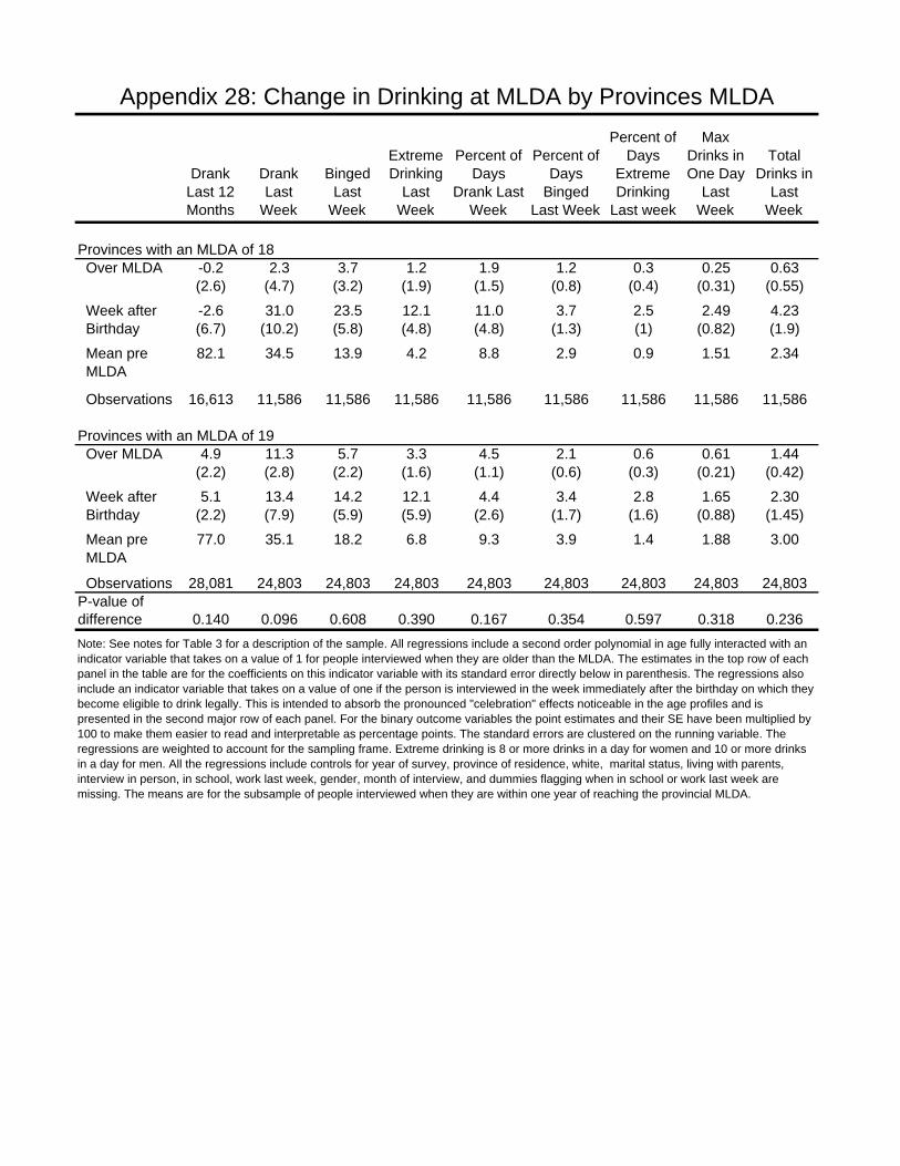
Drank Last 12 Months
Drank Last
Week
Binged Last
Week
Extreme Drinking
Last Week
Percent of Days
Drank Last Week
Percent of Days
Binged Last Week
Percent of Days
Extreme Drinking
Last week
Max Drinks in One Day
Last Week
Total Drinks in
Last Week
Provinces with an MLDA of 18 Over MLDA -0.2 2.3 3.7 1.2 1.9 1.2 0.3 0.25 0.63
(2.6) (4.7) (3.2) (1.9) (1.5) (0.8) (0.4) (0.31) (0.55)
Week after -2.6 31.0 23.5 12.1 11.0 3.7 2.5 2.49 4.23 Birthday (6.7) (10.2) (5.8) (4.8) (4.8) (1.3) (1) (0.82) (1.9)
Mean pre 82.1 34.5 13.9 4.2 8.8 2.9 0.9 1.51 2.34 MLDA
Observations 16,613 11,586 11,586 11,586 11,586 11,586 11,586 11,586 11,586
Provinces with an MLDA of 19 Over MLDA 4.9 11.3 5.7 3.3 4.5 2.1 0.6 0.61 1.44
(2.2) (2.8) (2.2) (1.6) (1.1) (0.6) (0.3) (0.21) (0.42)
Week after 5.1 13.4 14.2 12.1 4.4 3.4 2.8 1.65 2.30 Birthday (2.2) (7.9) (5.9) (5.9) (2.6) (1.7) (1.6) (0.88) (1.45)
Mean pre 77.0 35.1 18.2 6.8 9.3 3.9 1.4 1.88 3.00 MLDA Observations 28,081 24,803 24,803 24,803 24,803 24,803 24,803 24,803 24,803P-value ofdifference 0.140 0.096 0.608 0.390 0.167 0.354 0.597 0.318 0.236
Appendix 28: Change in Drinking at MLDA by Provinces MLDA
Note: See notes for Table 3 for a description of the sample. All regressions include a second order polynomial in age fully interacted with an indicator variable that takes on a value of 1 for people interviewed when they are older than the MLDA. The estimates in the top row of each panel in the table are for the coefficients on this indicator variable with its standard error directly below in parenthesis. The regressions also include an indicator variable that takes on a value of one if the person is interviewed in the week immediately after the birthday on which they become eligible to drink legally. This is intended to absorb the pronounced "celebration" effects noticeable in the age profiles and is presented in the second major row of each panel. For the binary outcome variables the point estimates and their SE have been multiplied by 100 to make them easier to read and interpretable as percentage points. The standard errors are clustered on the running variable. The regressions are weighted to account for the sampling frame. Extreme drinking is 8 or more drinks in a day for women and 10 or more drinks in a day for men. All the regressions include controls for year of survey, province of residence, white, marital status, living with parents, interview in person, in school, work last week, gender, month of interview, and dummies flagging when in school or work last week are missing. The means are for the subsample of people interviewed when they are within one year of reaching the provincial MLDA.

All Deaths Internal External Motor Vehicle Injuries
Weekend (Thursday to Sunday) Over MLDA 2.96 2.75 0.21 1.91 0.84
(0.09) (0.09) (0.74) (0.01) (0.49) Constant 31.88 22.85 9.03 10.88 11.97
Weekday (Monday to Wednesday) Over MLDA 1.15 2.46 -1.32 2.88 -0.42
(0.42) (0.05) (0.05) (0.01) (0.73) Constant 38.33 30.42 7.91 17.43 13.00
p-value of difference 0.413 0.886 0.098 0.463 0.461Observations 48 48 48 48 48
Appendix 29: Change in Death Rates Weekend vs. Weekday
Note: Each row presents the estimate of the increase in death rates for a particular cause when people become eligible to drink legally with the robust standard error of the estimate directly below in parenthesis. The estimates are from a regression with a second order polynomial in age fully interacted with an indicator variable equal to one for ages above the MLDA. The regressions also include an indicator variable for the month on which the MLDA birthday falls and are estimated with a two year bandwidth. Death rates are in deaths per 100,000 for each of the 48 month cells within 2 years of the MLDA. The constant is an estimate of the death rate just under the MLDA threshold. The causes of death are coded based on International Classification of Disease code and all causes of death fall into one of the three subcategories (Internal, Motor Vehicle Accident or Injuries). Mortality records provided by Statistics Canada. In the bottom row we present the p-value of the difference in the estimates of the MLDA effect.
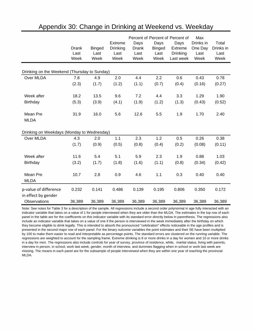
Drank Last
Week
Binged Last
Week
Extreme Drinking
Last Week
Percent of Days Drank Last
Week
Percent of Days
Binged Last
Week
Percent of Days
Extreme Drinking
Last week
Max Drinks in One Day
Last Week
Total Drinks in
Last Week
Drinking on the Weekend (Thursday to Sunday)
Over MLDA 7.8 4.9 2.0 4.4 2.2 0.6 0.43 0.78
(2.3) (1.7) (1.2) (1.1) (0.7) (0.4) (0.16) (0.27)
Week after 18.2 13.5 9.6 7.2 4.4 3.3 1.29 1.90
Birthday (5.3) (3.9) (4.1) (1.9) (1.2) (1.3) (0.43) (0.52)
Mean Pre 31.9 16.0 5.6 12.6 5.5 1.9 1.70 2.40
MLDA
Drinking on Weekdays (Monday to Wednesday)
Over MLDA 4.3 2.0 1.1 2.3 1.2 0.5 0.26 0.38
(1.7) (0.9) (0.5) (0.8) (0.4) (0.2) (0.08) (0.11)
Week after 11.6 5.4 5.1 5.9 2.3 1.9 0.88 1.03
Birthday (3.2) (1.7) (1.8) (1.6) (1.1) (0.8) (0.34) (0.42)
Mean Pre 10.7 2.8 0.9 4.6 1.1 0.3 0.40 0.40
MLDA
p‐value of difference 0.232 0.141 0.486 0.139 0.195 0.806 0.350 0.172
in effect by gender
Observations 36,389 36,389 36,389 36,389 36,389 36,389 36,389 36,389
Appendix 30: Change in Drinking at Weekend vs. Weekday
Note: See notes for Table 3 for a description of the sample. All regressions include a second order polynomial in age fully interacted with an indicator variable that takes on a value of 1 for people interviewed when they are older than the MLDA. The estimates in the top row of each panel in the table are for the coefficients on this indicator variable with its standard error directly below in parenthesis. The regressions also include an indicator variable that takes on a value of one if the person is interviewed in the week immediately after the birthday on which they become eligible to drink legally. This is intended to absorb the pronounced "celebration" effects noticeable in the age profiles and is presented in the second major row of each panel. For the binary outcome variables the point estimates and their SE have been multiplied by 100 to make them easier to read and interpretable as percentage points. The standard errors are clustered on the running variable. The regressions are weighted to account for the sampling frame. Extreme drinking is 8 or more drinks in a day for women and 10 or more drinks in a day for men. The regressions also include controls for year of survey, province of residence, white, marital status, living with parents, interview in person, in school, work last week, gender, month of interview, and dummies flagging when in school or work last week are missing. The means in each panel are for the subsample of people interviewed when they are within one year of reaching the provincial MLDA.