Mathematics Colloquium, UCSC
61
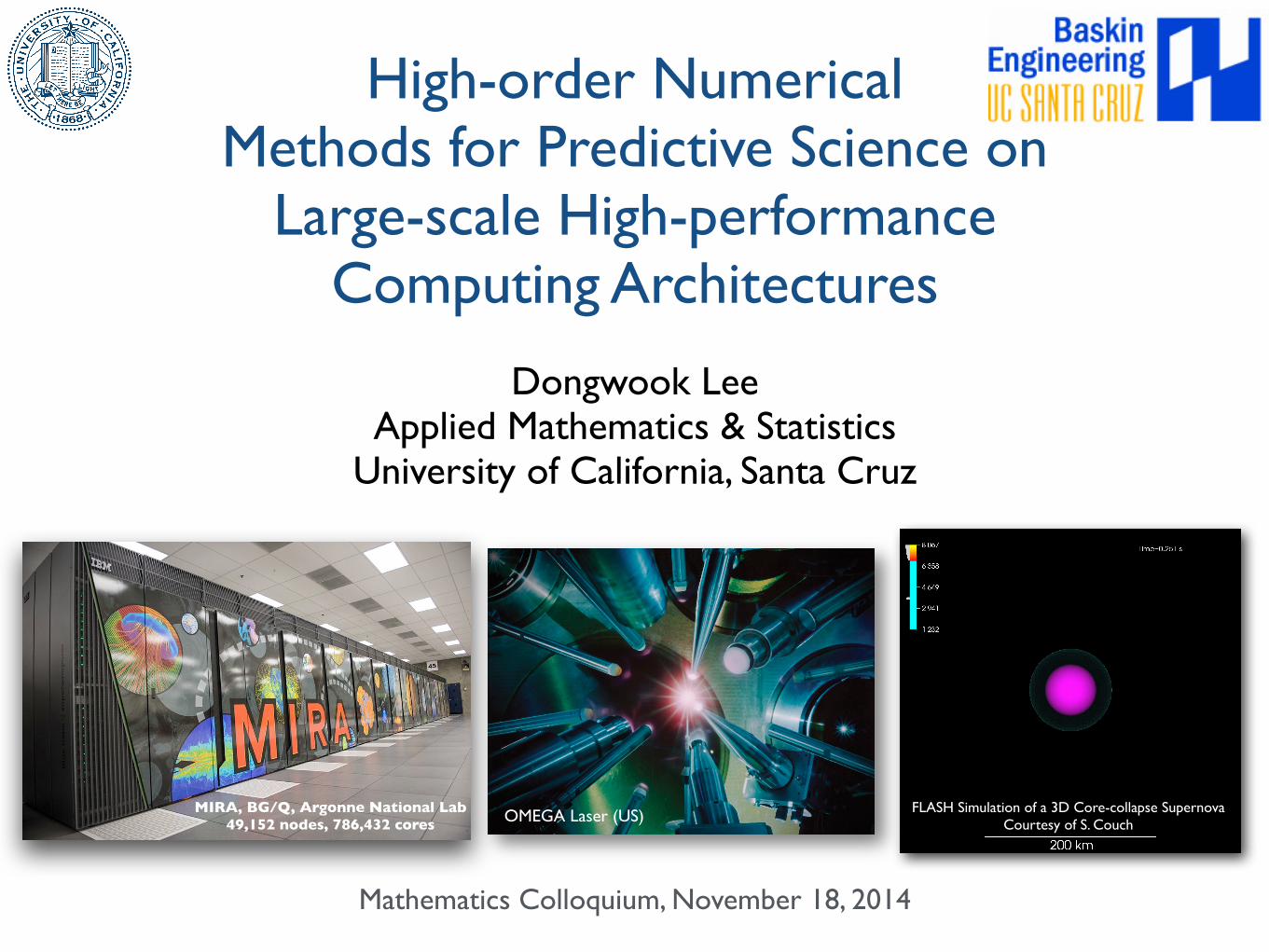
Dongwook Lee Applied Mathematics & Statistics University of California, Santa Cruz High-order Numerical Methods for Predictive Science on Large-scale High-performance Computing Architectures Mathematics Colloquium, November 18, 2014 FLASH Simulation of a 3D Core-collapse Supernova Courtesy of S. Couch MIRA, BG/Q, Argonne National Lab 49,152 nodes, 786,432 cores OMEGA Laser (US)
-
Upload
dongwook159 -
Category
Education
-
view
140 -
download
1
Transcript of Mathematics Colloquium, UCSC
Dongwook LeeApplied Mathematics & Statistics
University of California, Santa Cruz
High-order Numerical Methods for Predictive Science on
Large-scale High-performanceComputing Architectures
Mathematics Colloquium, November 18, 2014
FLASH Simulation of a 3D Core-collapse SupernovaCourtesy of S. Couch
MIRA, BG/Q, Argonne National Lab49,152 nodes, 786,432 cores OMEGA Laser (US)
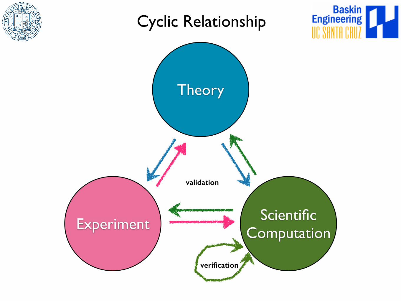
Theory
Experiment ScientificComputation
validation
verification
Cyclic Relationship
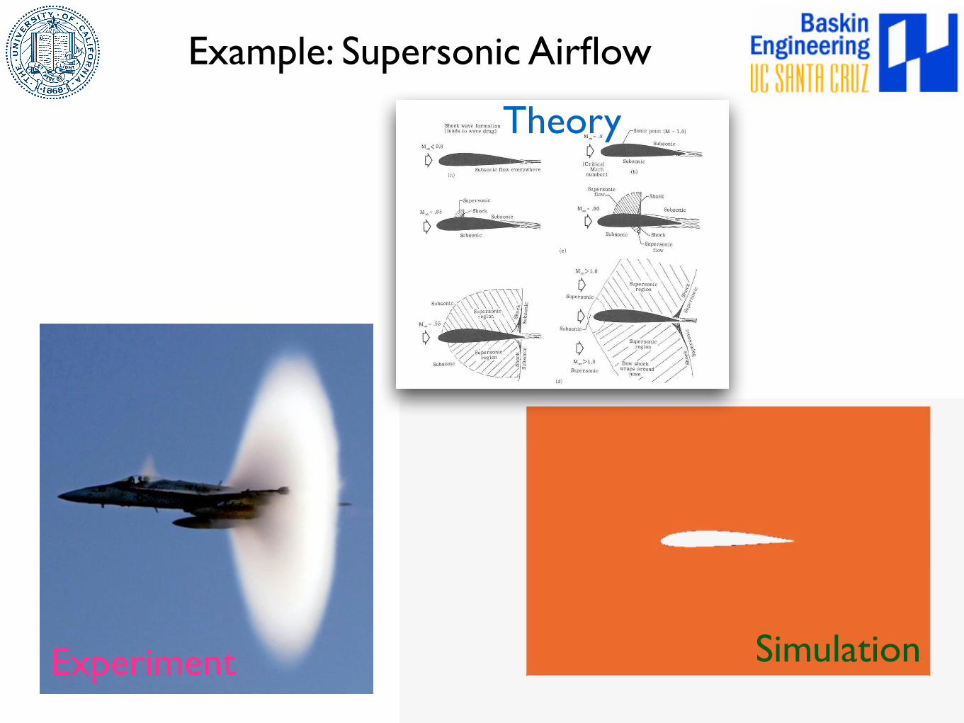
Example: Supersonic Airflow
Theory
Experiment Simulation

Topics for Today
1. High Performance Computing
2. Ideas on Numerical Methods
3. Validation & Predictive Science

First Episode
1. High Performance Computing
2. Ideas on Numerical Methods
3. Validation & Predictive Science
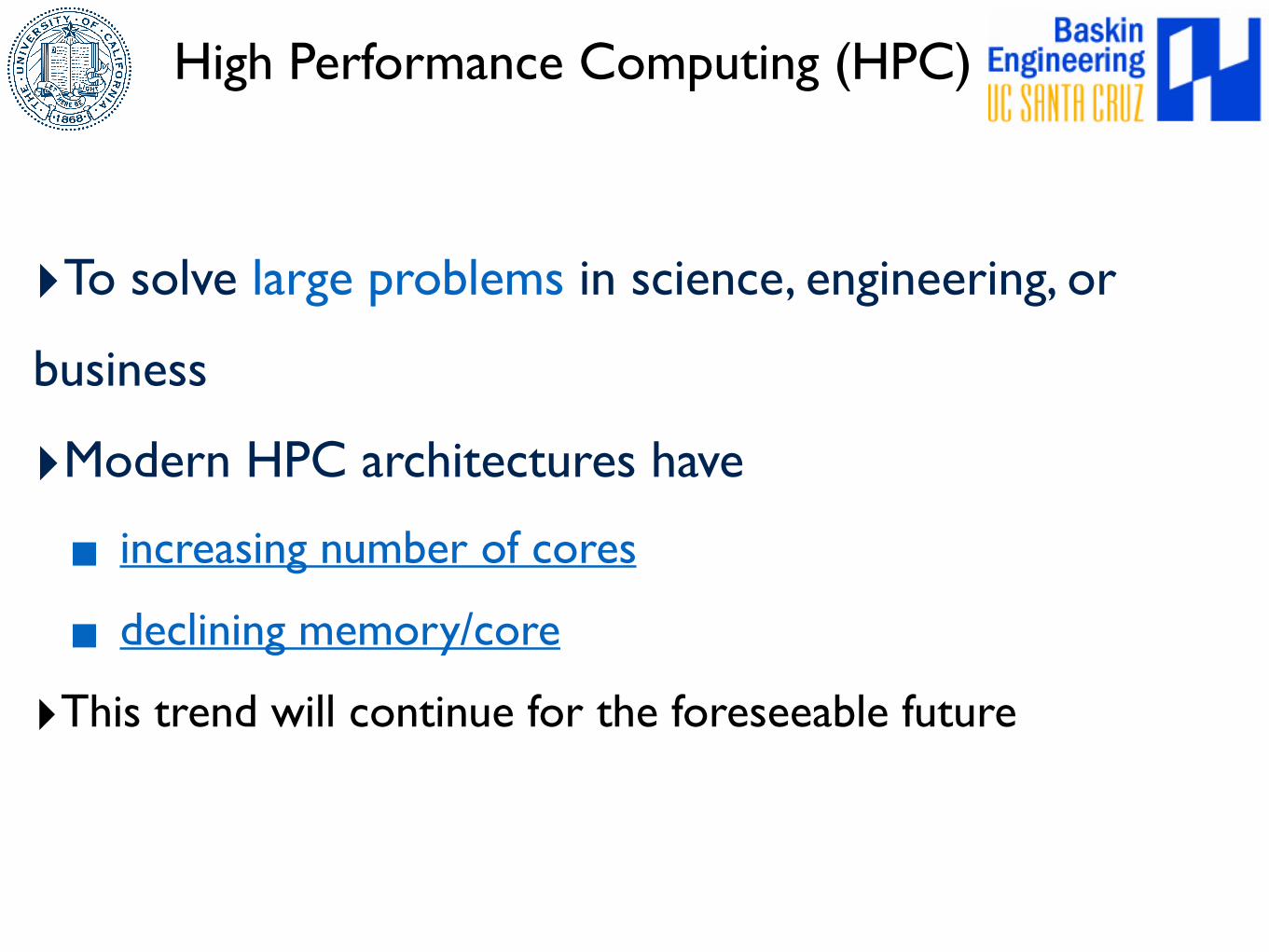
High Performance Computing (HPC)
‣To solve large problems in science, engineering, or
business
‣Modern HPC architectures have
▪ increasing number of cores
▪ declining memory/core
‣This trend will continue for the foreseeable future
High Performance Computing (HPC)
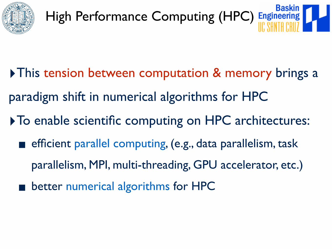
‣This tension between computation & memory brings a
paradigm shift in numerical algorithms for HPC
‣To enable scientific computing on HPC architectures:
▪ efficient parallel computing, (e.g., data parallelism, task
parallelism, MPI, multi-threading, GPU accelerator, etc.)
▪ better numerical algorithms for HPC
Numerical Algorithms for HPC
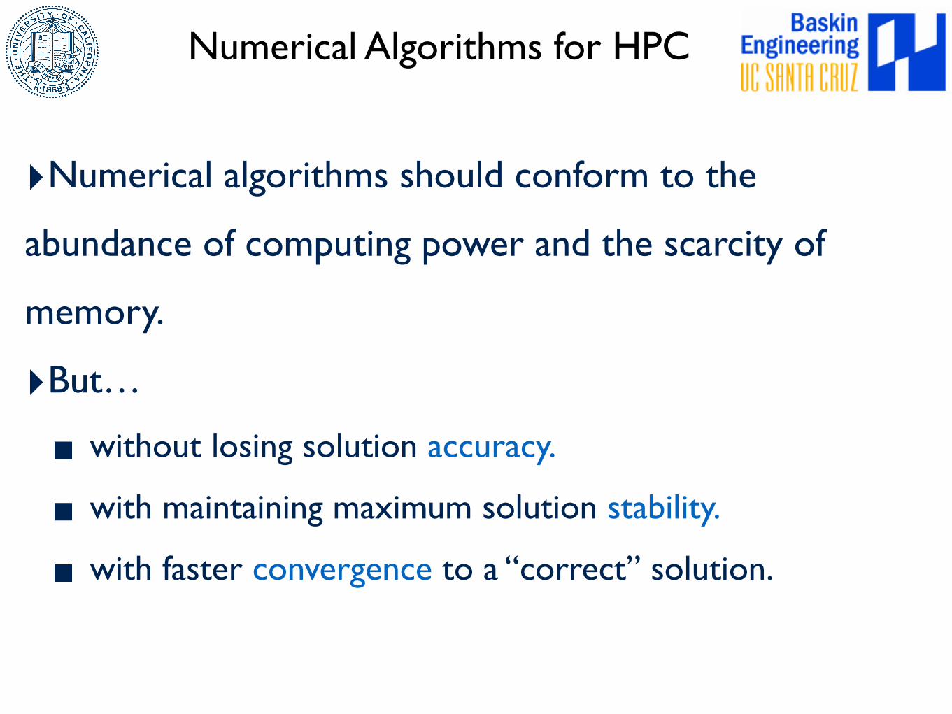
‣Numerical algorithms should conform to the
abundance of computing power and the scarcity of
memory.
‣But…
▪ without losing solution accuracy.
▪ with maintaining maximum solution stability.
▪ with faster convergence to a “correct” solution.
High-Order Numerical Algorithms
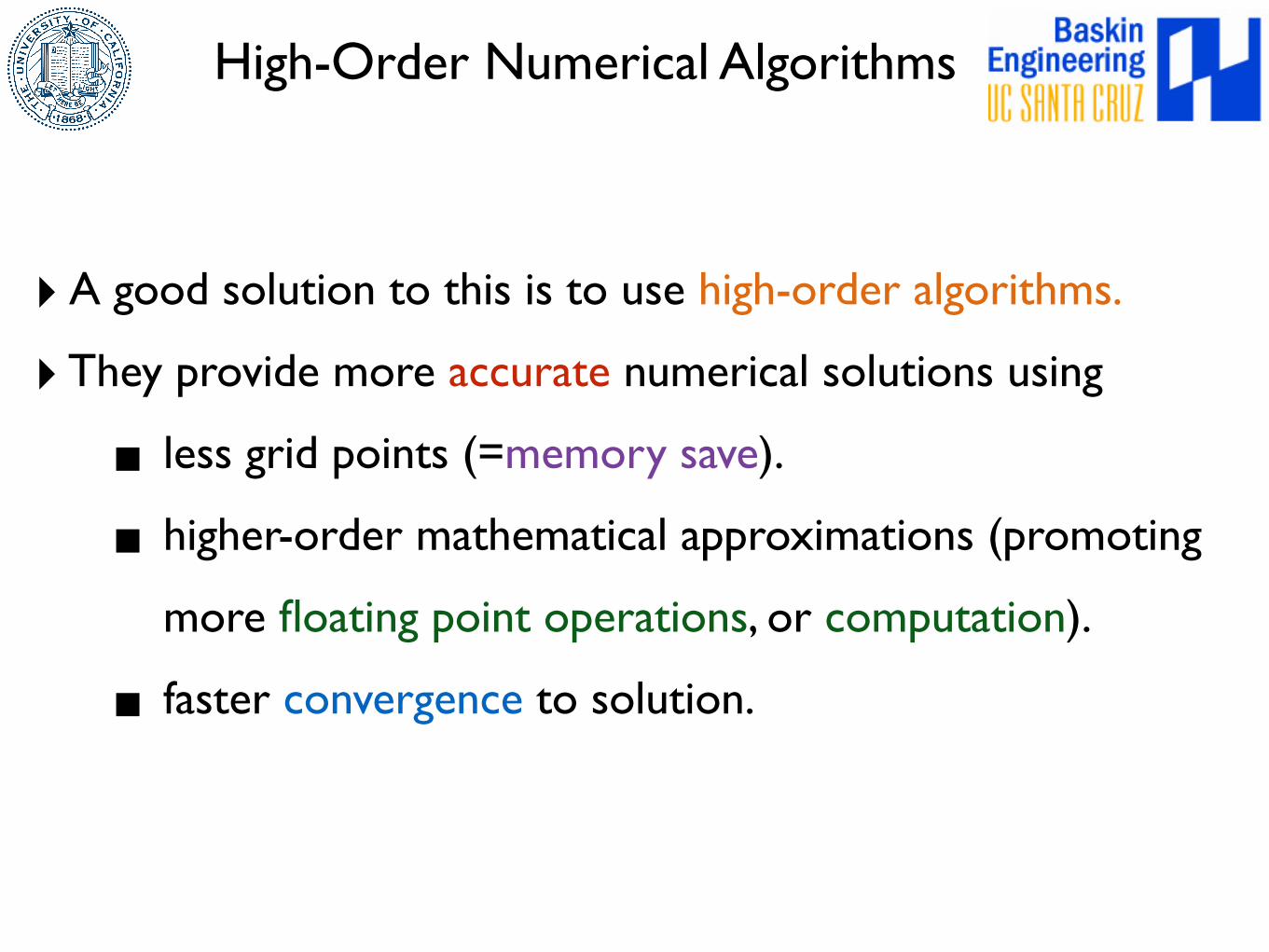
‣ A good solution to this is to use high-order algorithms.
‣ They provide more accurate numerical solutions using
▪ less grid points (=memory save).
▪ higher-order mathematical approximations (promoting
more floating point operations, or computation).
▪ faster convergence to solution.
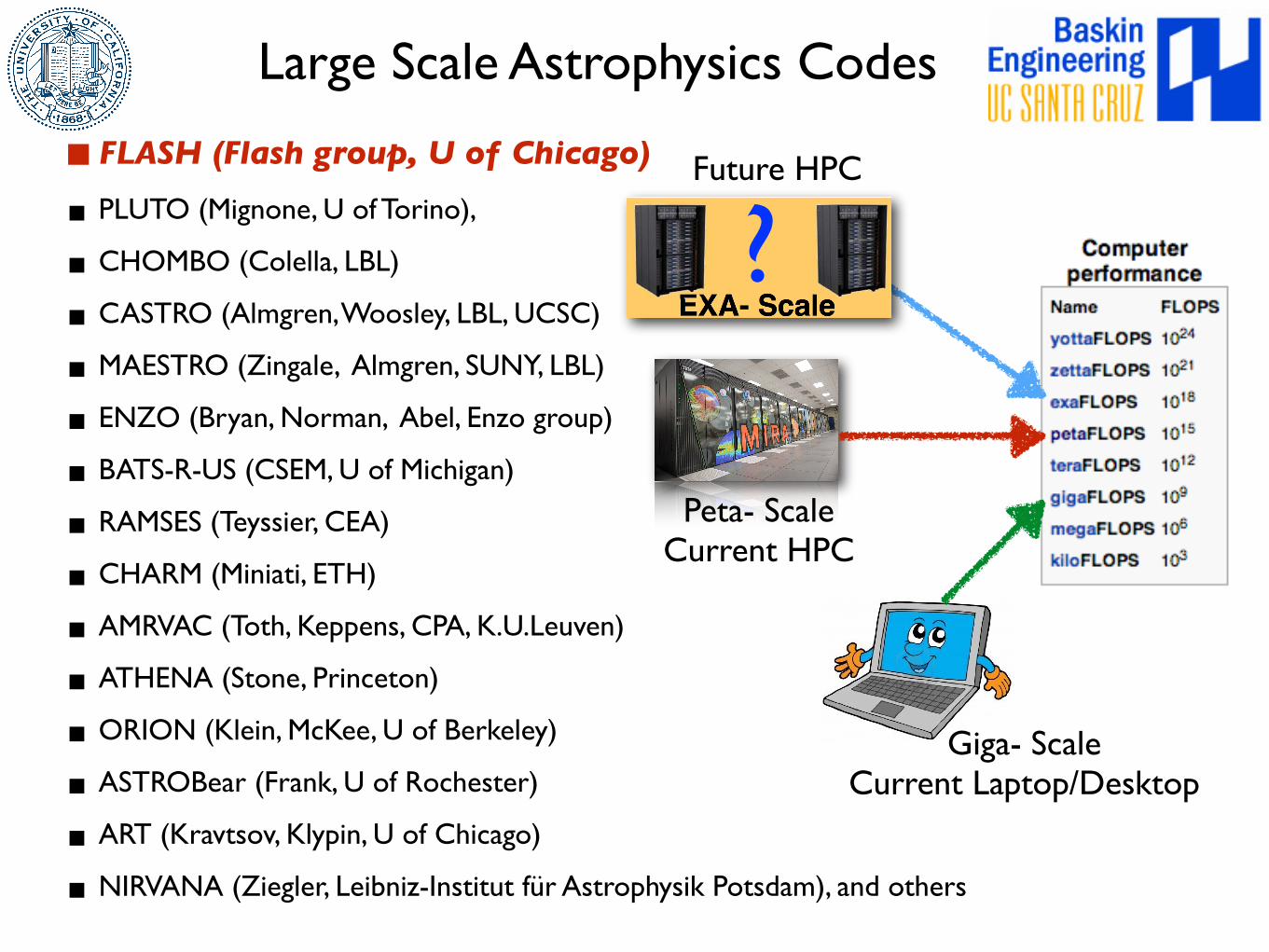
Large Scale Astrophysics Codes
▪ FLASH (Flash group, U of Chicago)
▪ PLUTO (Mignone, U of Torino),
▪ CHOMBO (Colella, LBL)
▪ CASTRO (Almgren, Woosley, LBL, UCSC)
▪ MAESTRO (Zingale, Almgren, SUNY, LBL)
▪ ENZO (Bryan, Norman, Abel, Enzo group)
▪ BATS-R-US (CSEM, U of Michigan)
▪ RAMSES (Teyssier, CEA)
▪ CHARM (Miniati, ETH)
▪ AMRVAC (Toth, Keppens, CPA, K.U.Leuven)
▪ ATHENA (Stone, Princeton)
▪ ORION (Klein, McKee, U of Berkeley)
▪ ASTROBear (Frank, U of Rochester)
▪ ART (Kravtsov, Klypin, U of Chicago)
▪ NIRVANA (Ziegler, Leibniz-Institut für Astrophysik Potsdam), and others
Peta- ScaleCurrent HPC
Future HPC
Giga- ScaleCurrent Laptop/Desktop
?
The FLASH Code
‣FLASH is is free, open source code for astrophysics and HEDP.
▪ modular, multi-physics, adaptive mesh refinement (AMR), parallel (MPI & OpenMP), finite-volume Eulerian compressible code for solving hydrodynamics and MHD
▪ professionally software engineered and maintained (daily regression test suite, code verification/validation), inline/online documentation
▪ 8500 downloads, 1500 authors, 1000 papers
▪ FLASH can run on various platforms from laptops to supercomputing (peta-scale) systems such as IBM BG/P and BG/Q.
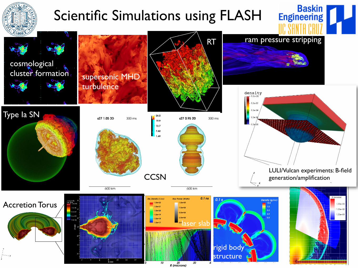
Scientific Simulations using FLASH
cosmological cluster formation supersonic MHD
turbulence
Type Ia SN
RT
CCSN
ram pressure stripping
laser slab
rigid body structure
Accretion Torus
LULI/Vulcan experiments: B-field generation/amplification
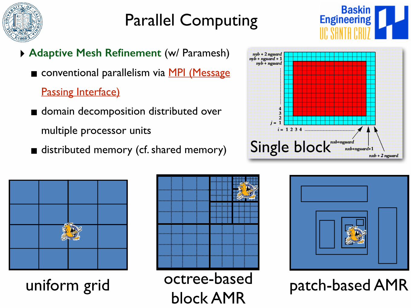
Parallel Computing
‣ Adaptive Mesh Refinement (w/ Paramesh)
▪ conventional parallelism via MPI (Message
Passing Interface)
▪ domain decomposition distributed over
multiple processor units
▪ distributed memory (cf. shared memory)
uniform grid octree-basedblock AMR
patch-based AMR
Single block
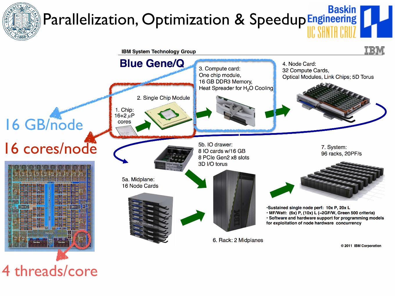
Parallelization, Optimization & Speedup
16 cores/node
16 GB/node
4 threads/core
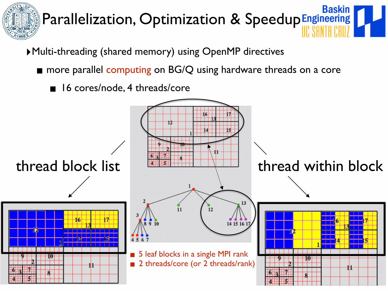
▪ 5 leaf blocks in a single MPI rank▪ 2 threads/core (or 2 threads/rank)
thread block list thread within block
‣Multi-threading (shared memory) using OpenMP directives
▪more parallel computing on BG/Q using hardware threads on a core
▪ 16 cores/node, 4 threads/core
Parallelization, Optimization & Speedup
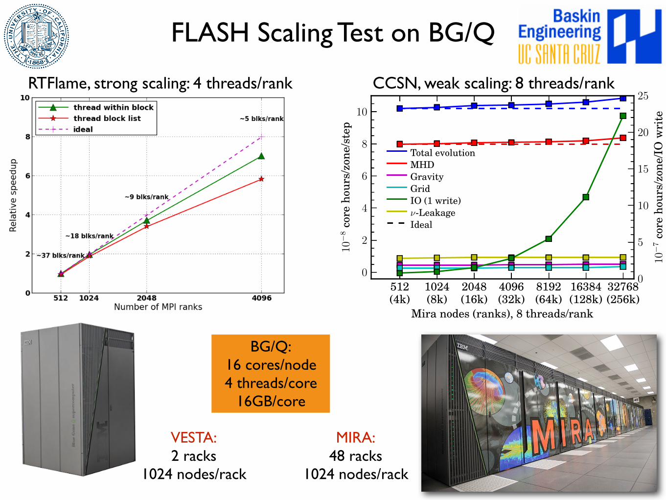
FLASH Scaling Test on BG/Q
VESTA:2 racks
1024 nodes/rack
MIRA:48 racks
1024 nodes/rack
BG/Q:16 cores/node4 threads/core
16GB/core
512(4k)
1024(8k)
2048(16k)
4096(32k)
8192(64k)
16384(128k)
32768(256k)
Mira nodes (ranks), 8 threads/rank
0
2
4
6
8
10
10�
8co
reho
urs/
zone
/ste
p
0
5
10
15
20
25
10�
7co
reho
urs/
zone
/IO
wri
te
Total evolutionMHDGravityGridIO (1 write)⌫-LeakageIdeal
RTFlame, strong scaling: 4 threads/rank CCSN, weak scaling: 8 threads/rank

Second Episode
1. High Performance Computing
2. Ideas on Numerical Methods
3. Validation & Predictive Science
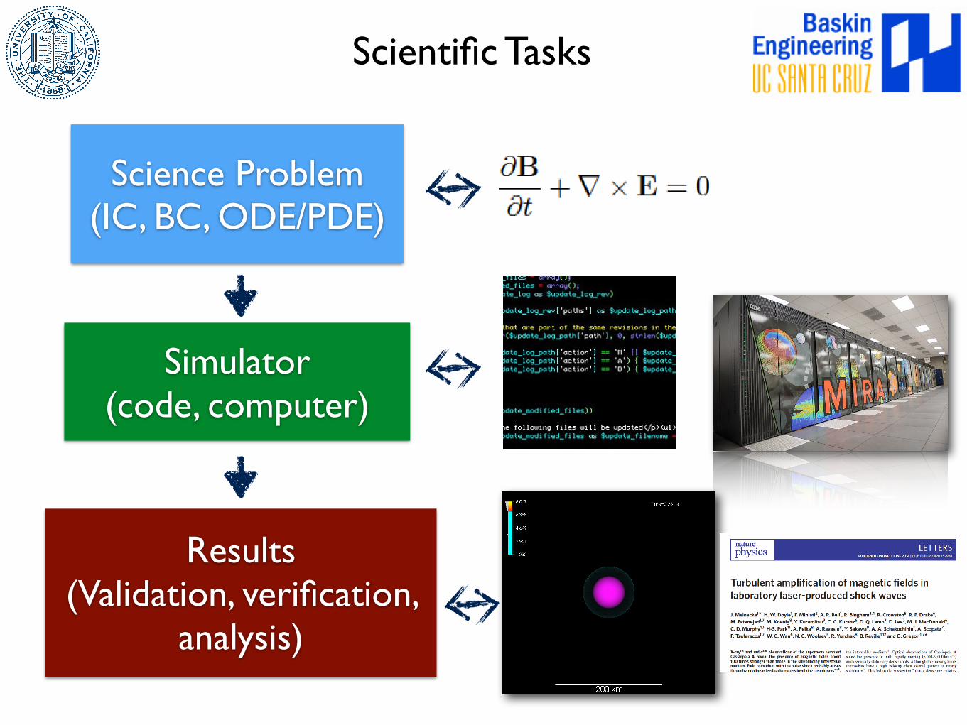
Scientific Tasks
Science Problem(IC, BC, ODE/PDE)
Simulator (code, computer)
Results(Validation, verification,
analysis)
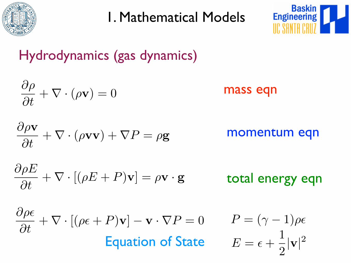
1. Mathematical Models
Hydrodynamics (gas dynamics)
@⇢
@t+r · (⇢v) = 0 mass eqn
@⇢v
@t+r · (⇢vv) +rP = ⇢g momentum eqn
@⇢E
@t+r · [(⇢E + P )v] = ⇢v · g total energy eqn
E = ✏+1
2|v|2
P = (� � 1)⇢✏@⇢✏
@t+r · [(⇢✏+ P )v]� v ·rP = 0
Equation of State
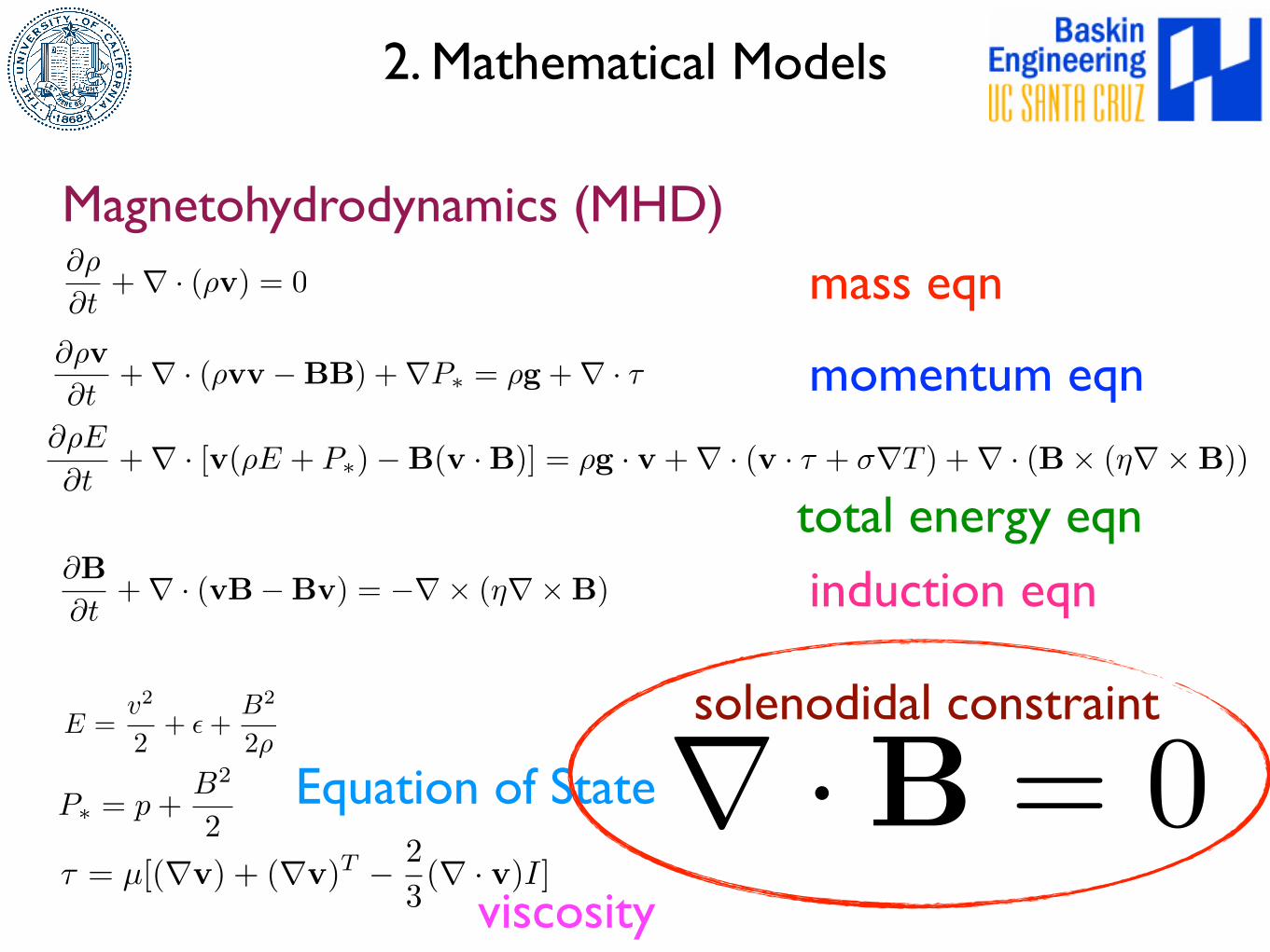
2. Mathematical Models
Magnetohydrodynamics (MHD)@⇢
@t+r · (⇢v) = 0 mass eqn
@⇢v
@t+r · (⇢vv �BB) +rP⇤ = ⇢g +r · ⌧ momentum eqn
@⇢E
@t+r · [v(⇢E + P⇤)�B(v ·B)] = ⇢g · v +r · (v · ⌧ + �rT ) +r · (B⇥ (⌘r⇥B))
total energy eqn@B
@t+r · (vB�Bv) = �r⇥ (⌘r⇥B) induction eqn
P⇤ = p+B2
2
E =v2
2+ ✏+
B2
2⇢
Equation of State
⌧ = µ[(rv) + (rv)T � 2
3(r · v)I]
viscosity
r ·B = 0solenodidal constraint
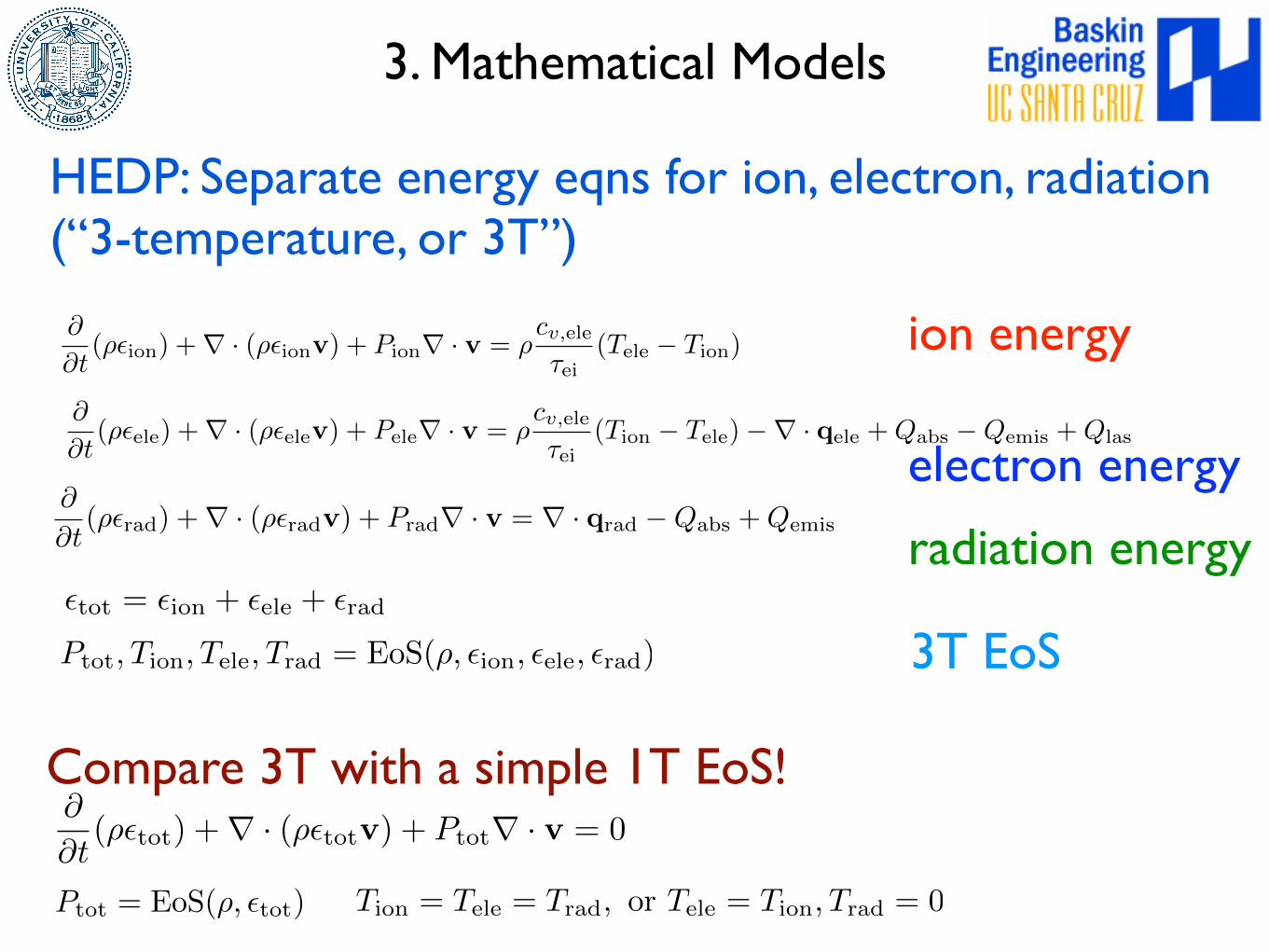
3. Mathematical Models
HEDP: Separate energy eqns for ion, electron, radiation (“3-temperature, or 3T”)
@
@t(⇢✏
ion
) +r · (⇢✏ion
v) + Pion
r · v = ⇢cv,ele⌧ei
(Tele
� Tion
) ion energy@
@t(⇢✏
ele
) +r · (⇢✏ele
v) + Pele
r · v = ⇢cv,ele⌧ei
(Tion
� Tele
)�r · qele
+Qabs
�Qemis
+Qlas
electron energy@
@t(⇢✏rad) +r · (⇢✏radv) + Pradr · v = r · qrad �Qabs +Qemis
radiation energy✏tot
= ✏ion
+ ✏ele
+ ✏rad
Ptot
, Tion
, Tele
, Trad
= EoS(⇢, ✏ion
, ✏ele
, ✏rad
) 3T EoS
Ptot
= EoS(⇢, ✏tot
)
@
@t(⇢✏
tot
) +r · (⇢✏tot
v) + Ptot
r · v = 0
Compare 3T with a simple 1T EoS!
Tion
= Tele
= Trad
, or Tele
= Tion
, Trad
= 0
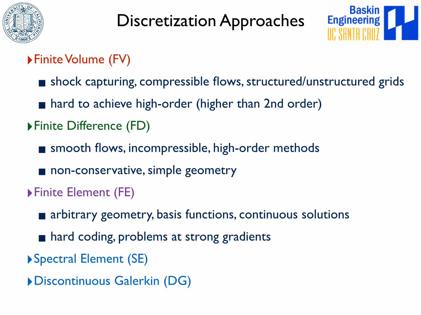
Discretization Approaches
‣Finite Volume (FV)
▪ shock capturing, compressible flows, structured/unstructured grids
▪ hard to achieve high-order (higher than 2nd order)
‣Finite Difference (FD)
▪ smooth flows, incompressible, high-order methods
▪ non-conservative, simple geometry
‣Finite Element (FE)
▪ arbitrary geometry, basis functions, continuous solutions
▪ hard coding, problems at strong gradients
‣Spectral Element (SE)
‣Discontinuous Galerkin (DG)
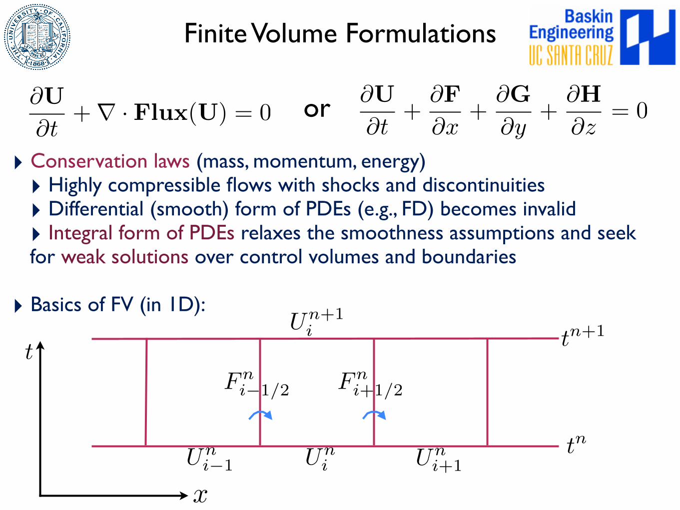
Finite Volume Formulations
@U
@t
+@F
@x
+@G
@y
+@H
@z
= 0@U
@t+r · Flux(U) = 0
‣ Conservation laws (mass, momentum, energy)‣ Highly compressible flows with shocks and discontinuities‣ Differential (smooth) form of PDEs (e.g., FD) becomes invalid‣ Integral form of PDEs relaxes the smoothness assumptions and seek for weak solutions over control volumes and boundaries
‣ Basics of FV (in 1D):
x
tUn+1i
Uni Un
i+1Uni�1
tn+1
tn
Fni�1/2 Fn
i+1/2
or
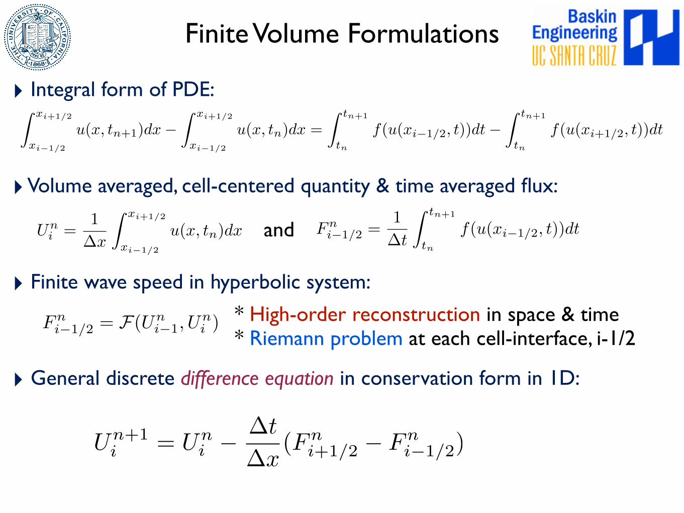
‣ Integral form of PDE:
‣ Volume averaged, cell-centered quantity & time averaged flux:
‣ Finite wave speed in hyperbolic system:
‣ General discrete difference equation in conservation form in 1D:
Finite Volume Formulations
Zxi+1/2
xi�1/2
u(x, tn+1)dx�
Zxi+1/2
xi�1/2
u(x, tn
)dx =
Ztn+1
tn
f(u(xi�1/2, t))dt�
Ztn+1
tn
f(u(xi+1/2, t))dt
U
n
i
=1
�x
Zxi+1/2
xi�1/2
u(x, tn
)dx F
ni�1/2 =
1
�t
Z tn+1
tn
f(u(xi�1/2, t))dtand
Fni�1/2 = F(Un
i�1, Uni )
* High-order reconstruction in space & time* Riemann problem at each cell-interface, i-1/2
U
n+1i = U
ni � �t
�x
(Fni+1/2 � F
ni�1/2)
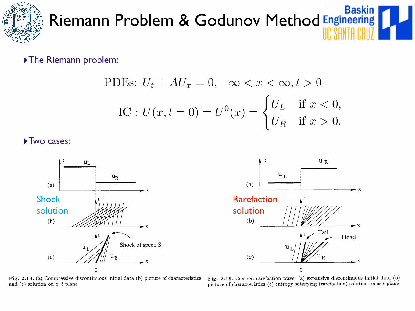
Riemann Problem & Godunov Method
‣The Riemann problem:
‣Two cases:
PDEs: Ut
+AU
x
= 0,�1 < x < 1, t > 0
IC : U(x, t = 0) = U
0(x) =
(U
L
if x < 0,
U
R
if x > 0.
Shock solution
Rarefaction solution
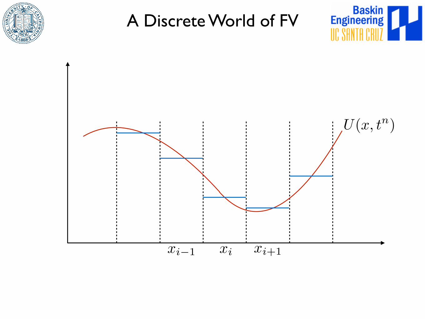
A Discrete World of FV
U(x, tn)
xixi�1 xi+1
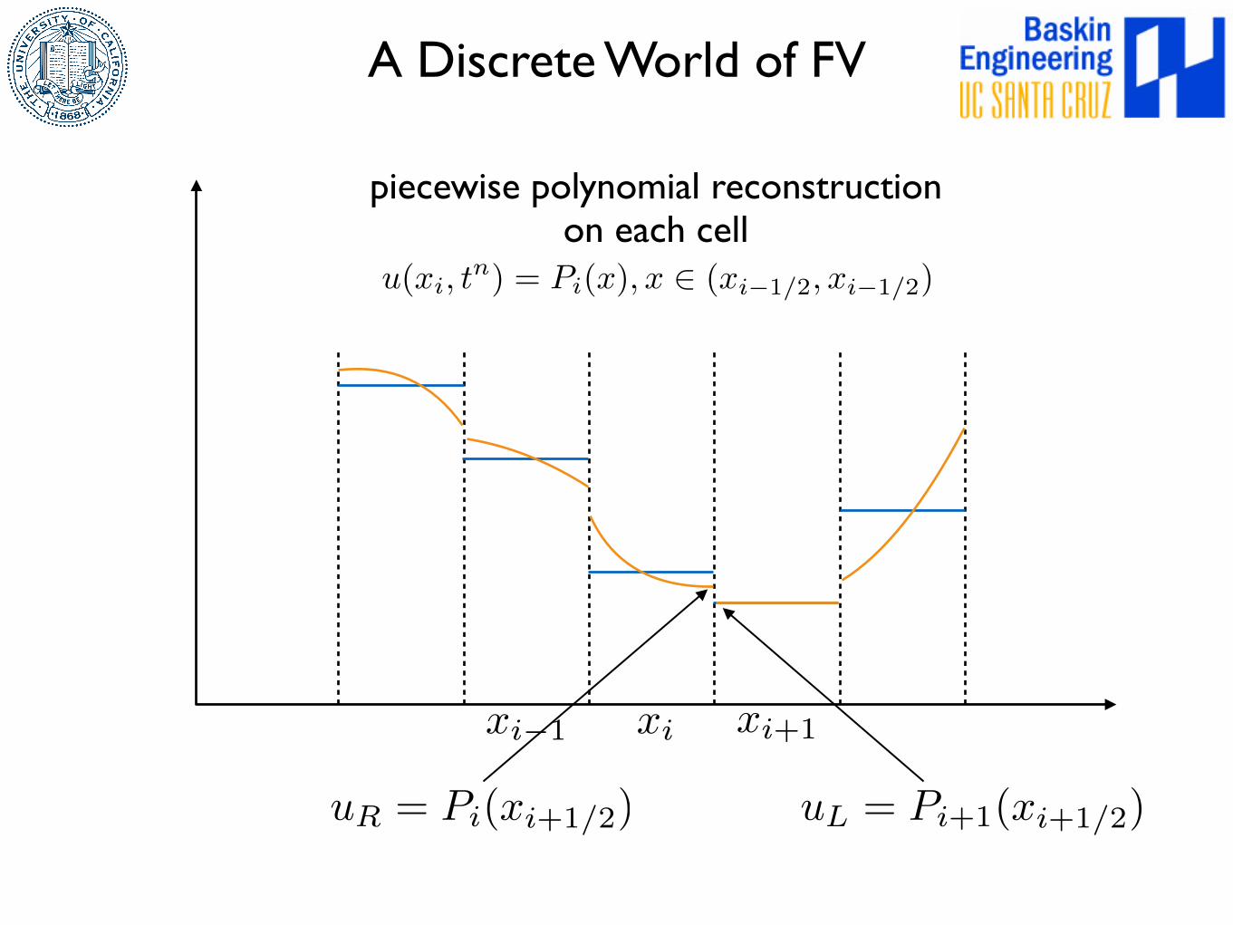
A Discrete World of FV
u(xi, tn) = Pi(x), x 2 (xi�1/2, xi�1/2)
xixi�1 xi+1
piecewise polynomial reconstruction on each cell
uL = Pi+1(xi+1/2)uR = Pi(xi+1/2)
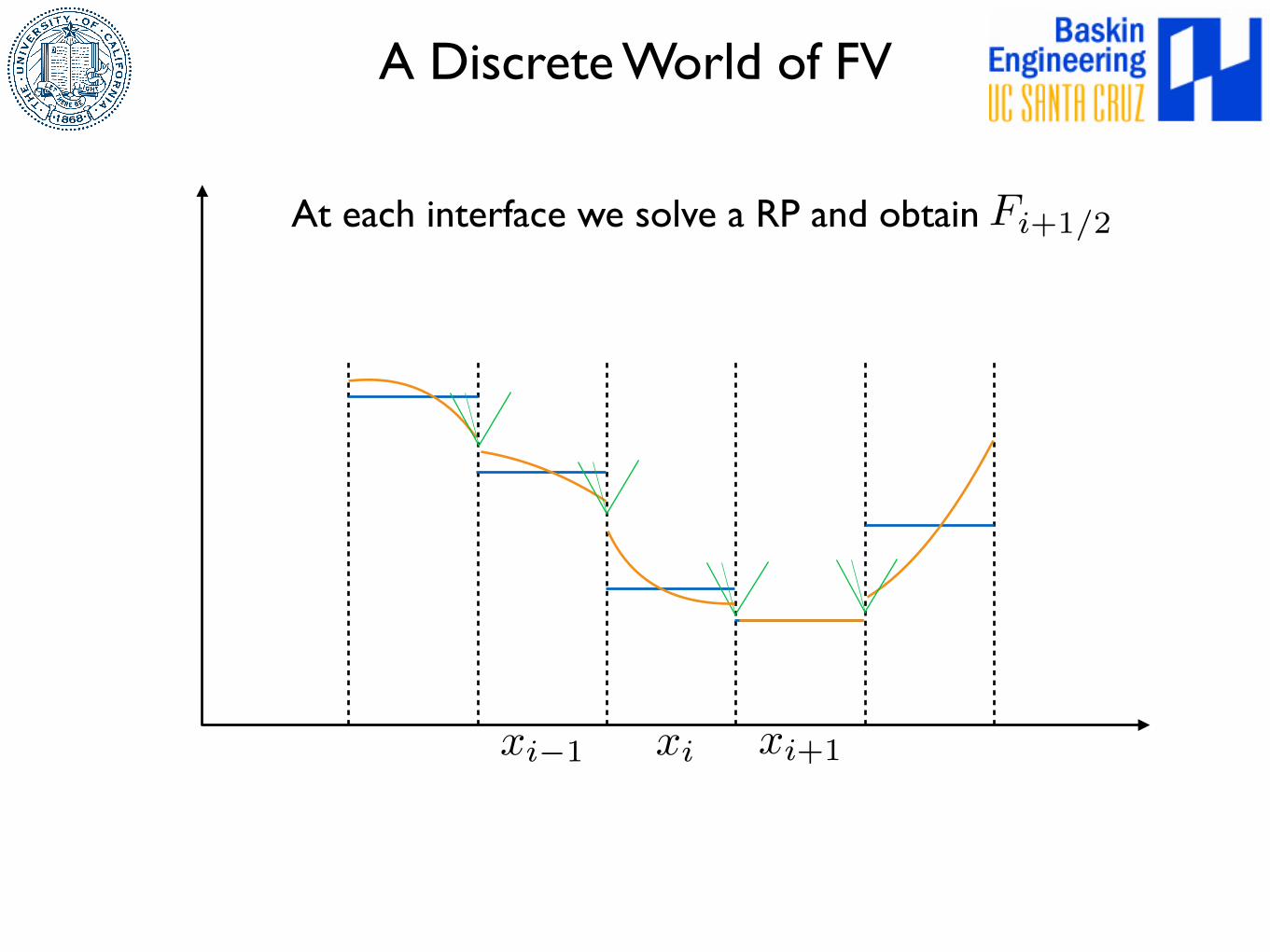
A Discrete World of FV
xixi�1 xi+1
At each interface we solve a RP and obtain Fi+1/2
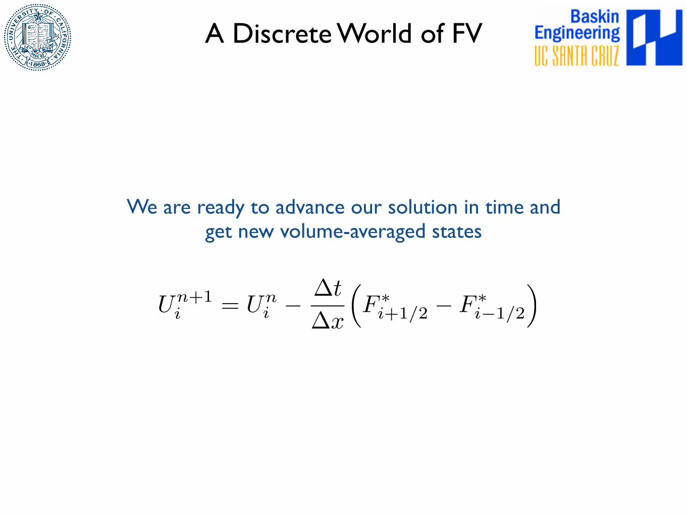
A Discrete World of FV
We are ready to advance our solution in time and get new volume-averaged states
U
n+1i = U
ni � �t
�x
⇣F
⇤i+1/2 � F
⇤i�1/2
⌘
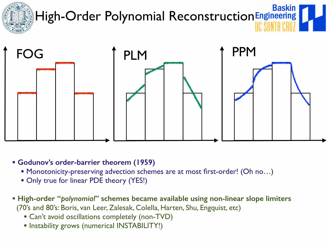
PLM PPM
High-Order Polynomial Reconstruction
• Godunov’s order-barrier theorem (1959) • Monotonicity-preserving advection schemes are at most first-order! (Oh no…)• Only true for linear PDE theory (YES!)
• High-order “polynomial” schemes became available using non-linear slope limiters (70’s and 80’s: Boris, van Leer, Zalesak, Colella, Harten, Shu, Engquist, etc)
• Can’t avoid oscillations completely (non-TVD)• Instability grows (numerical INSTABILITY!)
FOG
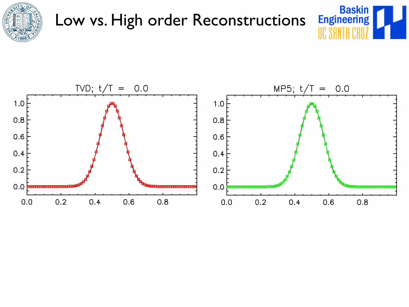
Low vs. High order Reconstructions
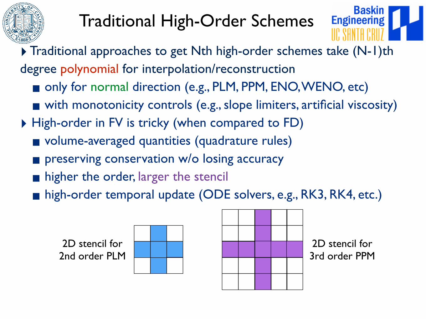
Traditional High-Order Schemes
‣ Traditional approaches to get Nth high-order schemes take (N-1)th degree polynomial for interpolation/reconstruction
▪ only for normal direction (e.g., PLM, PPM, ENO, WENO, etc)
▪with monotonicity controls (e.g., slope limiters, artificial viscosity)
‣ High-order in FV is tricky (when compared to FD)
▪ volume-averaged quantities (quadrature rules)
▪ preserving conservation w/o losing accuracy
▪ higher the order, larger the stencil
▪ high-order temporal update (ODE solvers, e.g., RK3, RK4, etc.)
2D stencil for 2nd order PLM
2D stencil for 3rd order PPM
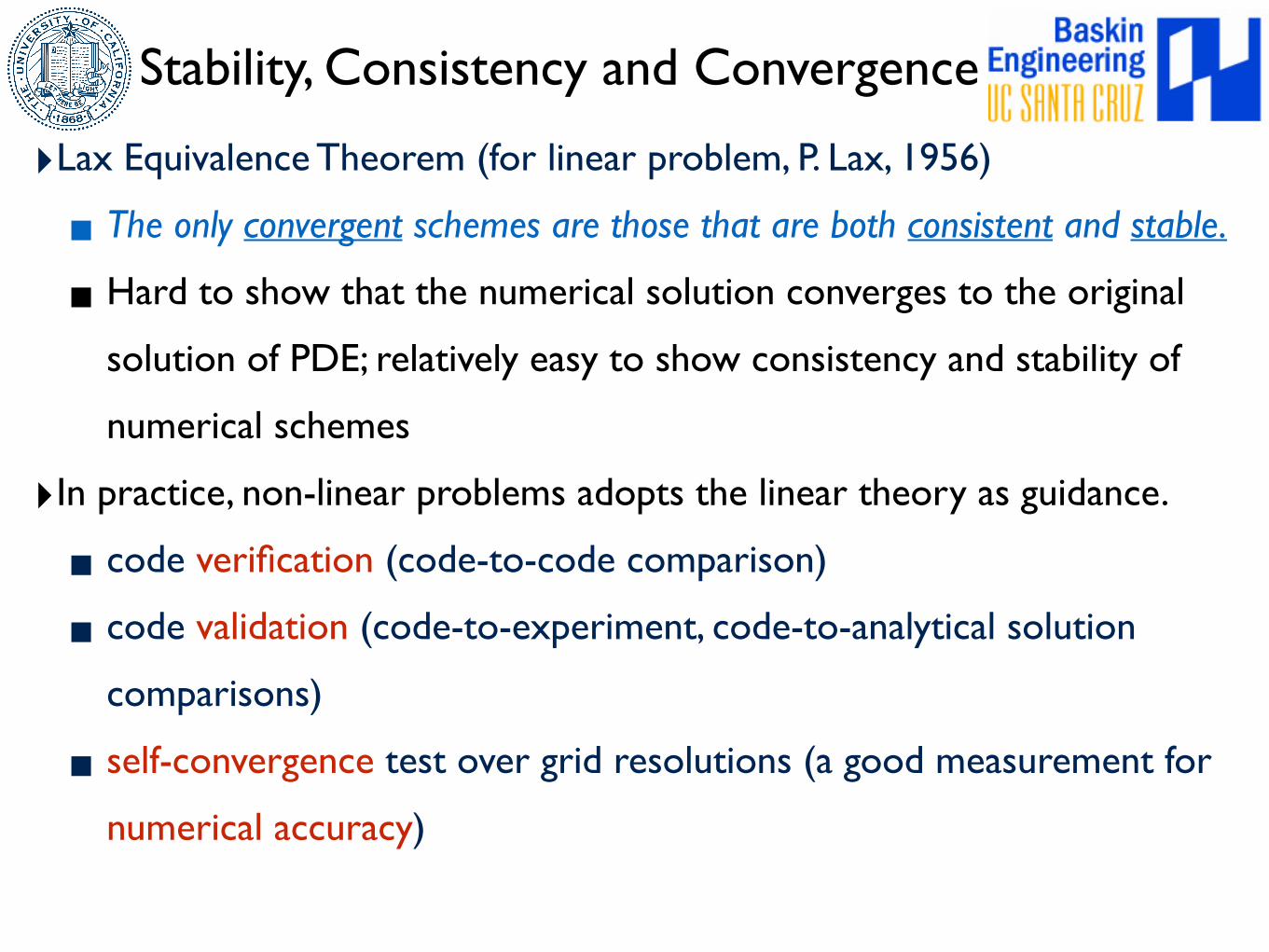
Stability, Consistency and Convergence
‣Lax Equivalence Theorem (for linear problem, P. Lax, 1956)
▪ The only convergent schemes are those that are both consistent and stable.
▪Hard to show that the numerical solution converges to the original
solution of PDE; relatively easy to show consistency and stability of
numerical schemes
‣In practice, non-linear problems adopts the linear theory as guidance.
▪ code verification (code-to-code comparison)
▪ code validation (code-to-experiment, code-to-analytical solution
comparisons)
▪ self-convergence test over grid resolutions (a good measurement for
numerical accuracy)
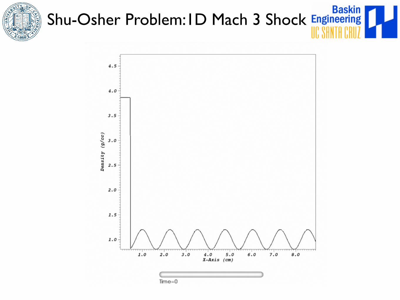
Shu-Osher Problem:1D Mach 3 Shock
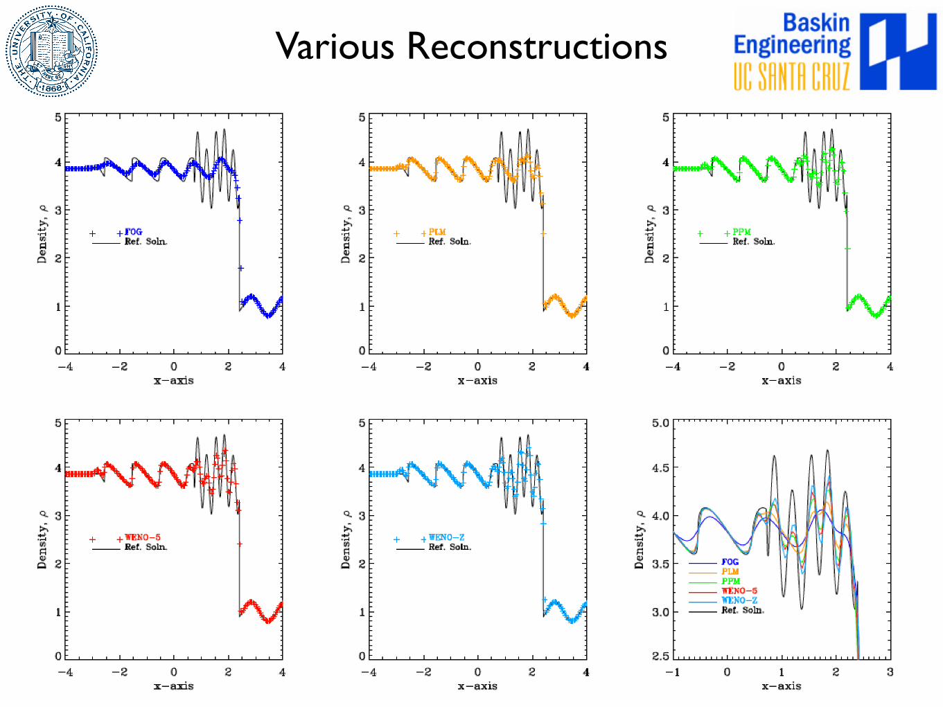
Various Reconstructions
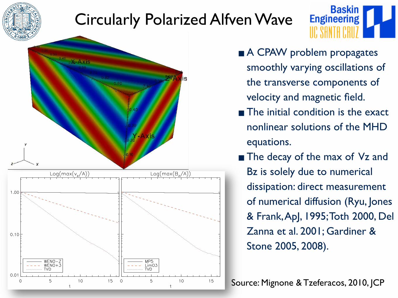
Circularly Polarized Alfven Wave
▪A CPAW problem propagates smoothly varying oscillations of the transverse components of velocity and magnetic field.
▪The initial condition is the exact nonlinear solutions of the MHD equations.
▪The decay of the max of Vz and Bz is solely due to numerical dissipation: direct measurement of numerical diffusion (Ryu, Jones & Frank, ApJ, 1995; Toth 2000, Del Zanna et al. 2001; Gardiner & Stone 2005, 2008).
These results are in agreement with previous investigations [5,6] and strongly supports the idea that problems involvingcomplex wave interactions may benefit from using higher-order schemes such as the ones presented here.
4.2. Shock tube problems
Shock tube problems are commonly used to test the ability of the scheme in describing both continuous and discontin-uous flow features. In the following we consider two- and three-dimensional rotated configurations of standard one-dimen-sional tubes. The default value for the parameter ap controlling monopole damping (see Eq. (9)) is 0.8.
4.2.1. Two-dimensional shock tubeFollowing [30,33], we consider a rotated version of the Brio-Wu test problem [8] with left and right states are given by
VL ¼ ð1; 0;0; 0:75;1;1ÞT for x1 < 0;
VR ¼ ð0:125;0;0;0:75;$1;0:1ÞT for x1 > 0;
(ð49Þ
where V ¼ ðq; v1;v2;B1;B2; pÞ is the vector of primitive variables. The subscript ‘‘1” gives the direction perpendicular to theinitial surface of discontinuity whereas ‘‘2” corresponds to the transverse direction. Here C = 2 is used and the evolution isinterrupted at time t = 0.2, before the fast waves reach the borders.
In order to address the ability to preserve the initial planar symmetry we rotate the initial condition by the angle a ¼ p=4in a two-dimensional plane with x 2 ½$1;1& and y 2 ½$0:01;0:01& using Nx ' Nx=100 grid points, with Nx = 600. Vectors followthe same transformation given by Eq. (45) with b = c = 0. This is known to minimize errors of the longitudinal component ofthe magnetic field (see for example the discussions in [52,27]). Boundary conditions respect the translational invariancespecified by the rotation: for each flow quantity we prescribe qði; jÞ ¼ qði( di; j( djÞ where ðdi; djÞ ¼ ð1;$1Þ, with the plus(minus) sign for the leftmost and upper (rightmost and lower) boundary. Computations are stopped before the fast rarefac-tion waves reach the boundaries, at t ¼ 0:2 cos a.
Fig. A.4 shows the primitive variable profiles for all schemes against a one-dimensional reference solution obtained on abase grid of 1024 zones with five levels of refinement. Errors in L1 norm, computed with respect to the same reference solu-tion, are sorted in Table 2 for density and the normal component of magnetic field. The out-coming wave pattern is com-prised, from left to right, of a fast rarefaction, a compound wave (an intermediate shock followed by a slow rarefaction),a contact discontinuity, a slow shock and a fast rarefaction wave. We see that all discontinuities are captured correctlyand the overall behavior matches the reference solution very well. The normal component of magnetic field is best describedwith MP5 and does not show erroneous jumps. Indeed, the profiles are essentially constant with small amplitude oscillationsshowing a relative peak )0.7%. Divergence errors, typically K 10$2, remain bounded with resolution and tend to saturate
Fig. A.3. Long term decay of circularly polarized Alfvén waves after 16.5 time units, corresponding to ) 100 wave periods. In the left panel, we plot themaximum value of the vertical component of velocity as a function of time for the WENO $ Z (solid line) and WENO + 3 (dashed line) schemes. Forcomparison, the dotted line gives the result obtained by a second-order TVD scheme. The panel on the right shows the analogous behavior of the verticalcomponent of magnetic field Bz for LimO3 and MP5. For all cases, the resolution was set to 120 ' 20 and the Courant number is 0.4.
A. Mignone et al. / Journal of Computational Physics 229 (2010) 5896–5920 5907
Source: Mignone & Tzeferacos, 2010, JCP
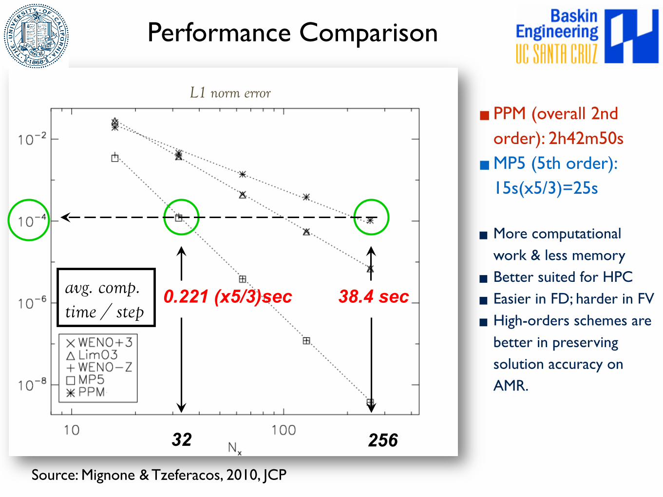
Performance Comparison
L1 norm error
avg. comp. time / step
32 256
0.221 (x5/3)sec 38.4 sec
Source: Mignone & Tzeferacos, 2010, JCP
▪PPM (overall 2nd order): 2h42m50s
▪MP5 (5th order): 15s(x5/3)=25s
▪More computational work & less memory
▪ Better suited for HPC
▪ Easier in FD; harder in FV
▪High-orders schemes are better in preserving solution accuracy on AMR.
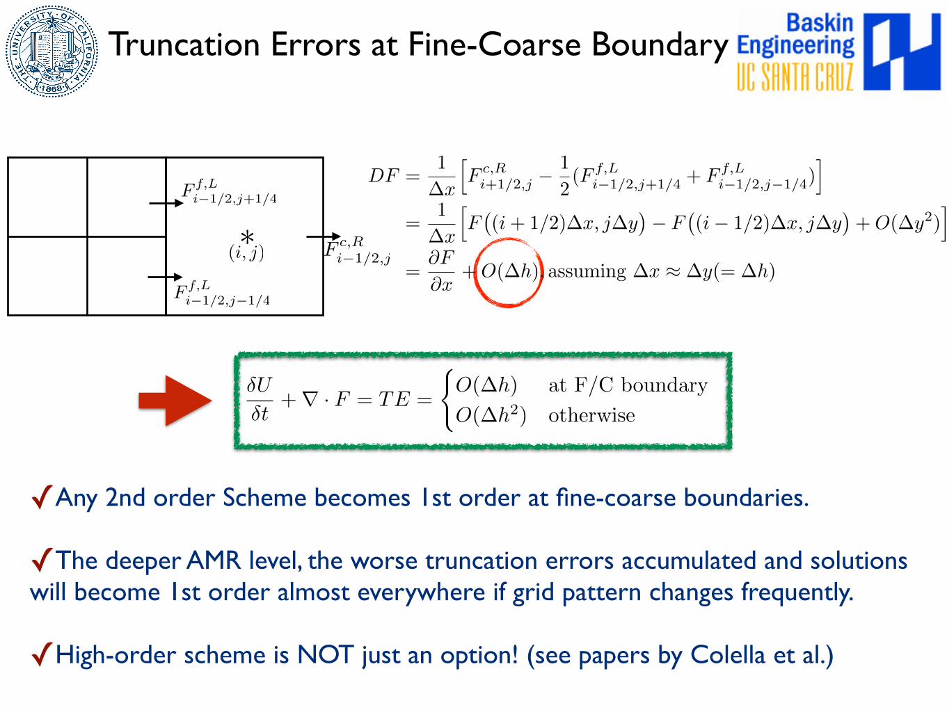
Truncation Errors at Fine-Coarse Boundary
✓Any 2nd order Scheme becomes 1st order at fine-coarse boundaries.
✓The deeper AMR level, the worse truncation errors accumulated and solutions will become 1st order almost everywhere if grid pattern changes frequently.
✓High-order scheme is NOT just an option! (see papers by Colella et al.)
F f,Li�1/2,j+1/4
F f,Li�1/2,j�1/4
F c,Ri�1/2,j(i, j)
⇤
�U
�t+r · F = TE =
(O(�h) at F/C boundary
O(�h2) otherwise
DF =1
�x
hF c,Ri+1/2,j �
1
2(F f,L
i�1/2,j+1/4 + F f,Li�1/2,j�1/4)
i
=1
�x
hF�(i+ 1/2)�x, j�y
�� F
�(i� 1/2)�x, j�y
�+O(�y2)
i
=@F
@x+O(�h), assuming �x ⇡ �y(= �h)
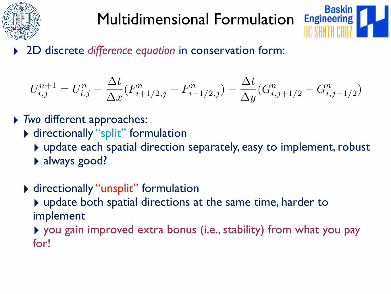
Multidimensional Formulation
‣ 2D discrete difference equation in conservation form:
‣ Two different approaches:‣ directionally “split” formulation‣ update each spatial direction separately, easy to implement, robust‣ always good?
‣ directionally “unsplit” formulation‣ update both spatial directions at the same time, harder to implement‣ you gain improved extra bonus (i.e., stability) from what you pay for!
U
n+1i,j = U
ni,j �
�t
�x
(Fni+1/2,j � F
ni�1/2,j)�
�t
�y
(Gni,j+1/2 �G
ni,j�1/2)
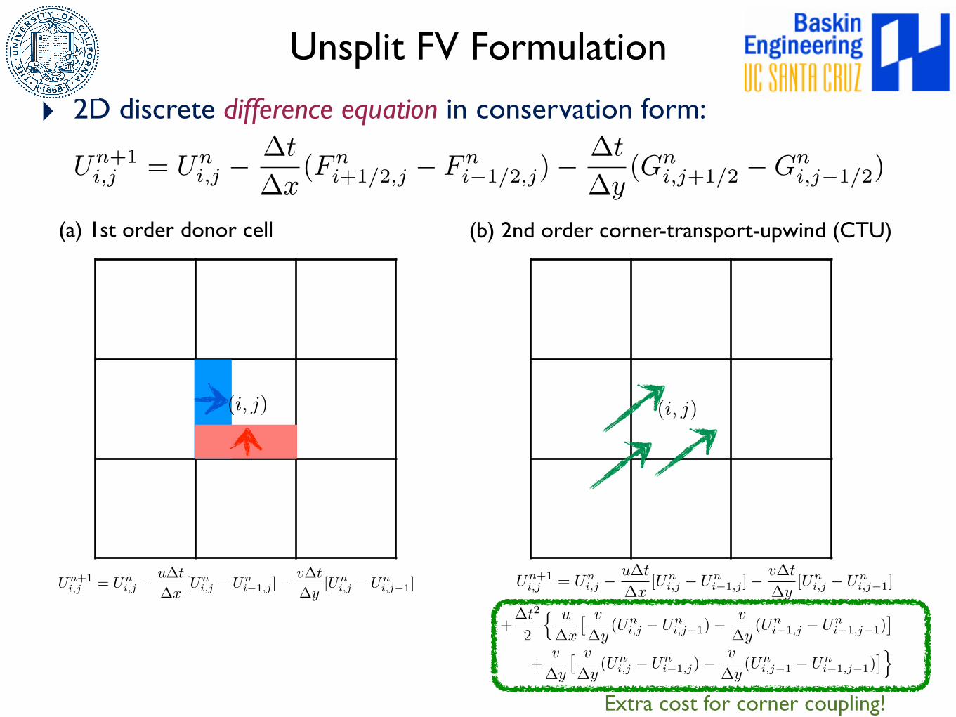
Unsplit FV Formulation
‣ 2D discrete difference equation in conservation form:
U
n+1i,j = U
ni,j �
u�t
�x
[Uni,j � U
ni�1,j ]�
v�t
�y
[Uni,j � U
ni,j�1] U
n+1i,j = U
ni,j �
u�t
�x
[Uni,j � U
ni�1,j ]�
v�t
�y
[Uni,j � U
ni,j�1]
+�t
2
2
n
u
�x
⇥
v
�y
(Uni,j � U
ni,j�1)�
v
�y
(Uni�1,j � U
ni�1,j�1)
⇤
+v
�y
⇥
v
�y
(Uni,j � U
ni�1,j)�
v
�y
(Uni,j�1 � U
ni�1,j�1)
⇤
o
Extra cost for corner coupling!
(a) 1st order donor cell
(i, j)
U
n+1i,j = U
ni,j �
�t
�x
(Fni+1/2,j � F
ni�1/2,j)�
�t
�y
(Gni,j+1/2 �G
ni,j�1/2)
(b) 2nd order corner-transport-upwind (CTU)
(i, j)
Unsplit FV Formulation
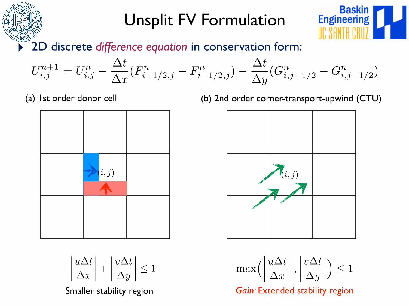
‣ 2D discrete difference equation in conservation form:
U
n+1i,j = U
ni,j �
�t
�x
(Fni+1/2,j � F
ni�1/2,j)�
�t
�y
(Gni,j+1/2 �G
ni,j�1/2)
����u�t
�x
����+����v�t
�y
���� 1max
⇣����u�t
�x
���� ,����v�t
�y
����⌘ 1
Smaller stability region Gain: Extended stability region
(a) 1st order donor cell
(i, j)
(b) 2nd order corner-transport-upwind (CTU)
(i, j)
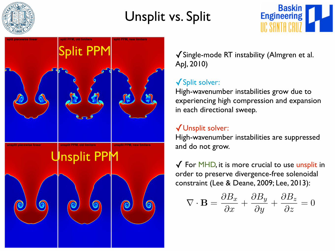
Unsplit vs. Split
✓Single-mode RT instability (Almgren et al. ApJ, 2010)
✓Split solver:High-wavenumber instabilities grow due to experiencing high compression and expansion in each directional sweep.
✓Unsplit solver:High-wavenumber instabilities are suppressed and do not grow.
✓ For MHD, it is more crucial to use unsplit in order to preserve divergence-free solenoidal constraint (Lee & Deane, 2009; Lee, 2013):
Split PPM
Unsplit PPM
r ·B =@B
x
@x
+@B
y
@y
+@B
z
@z
= 0
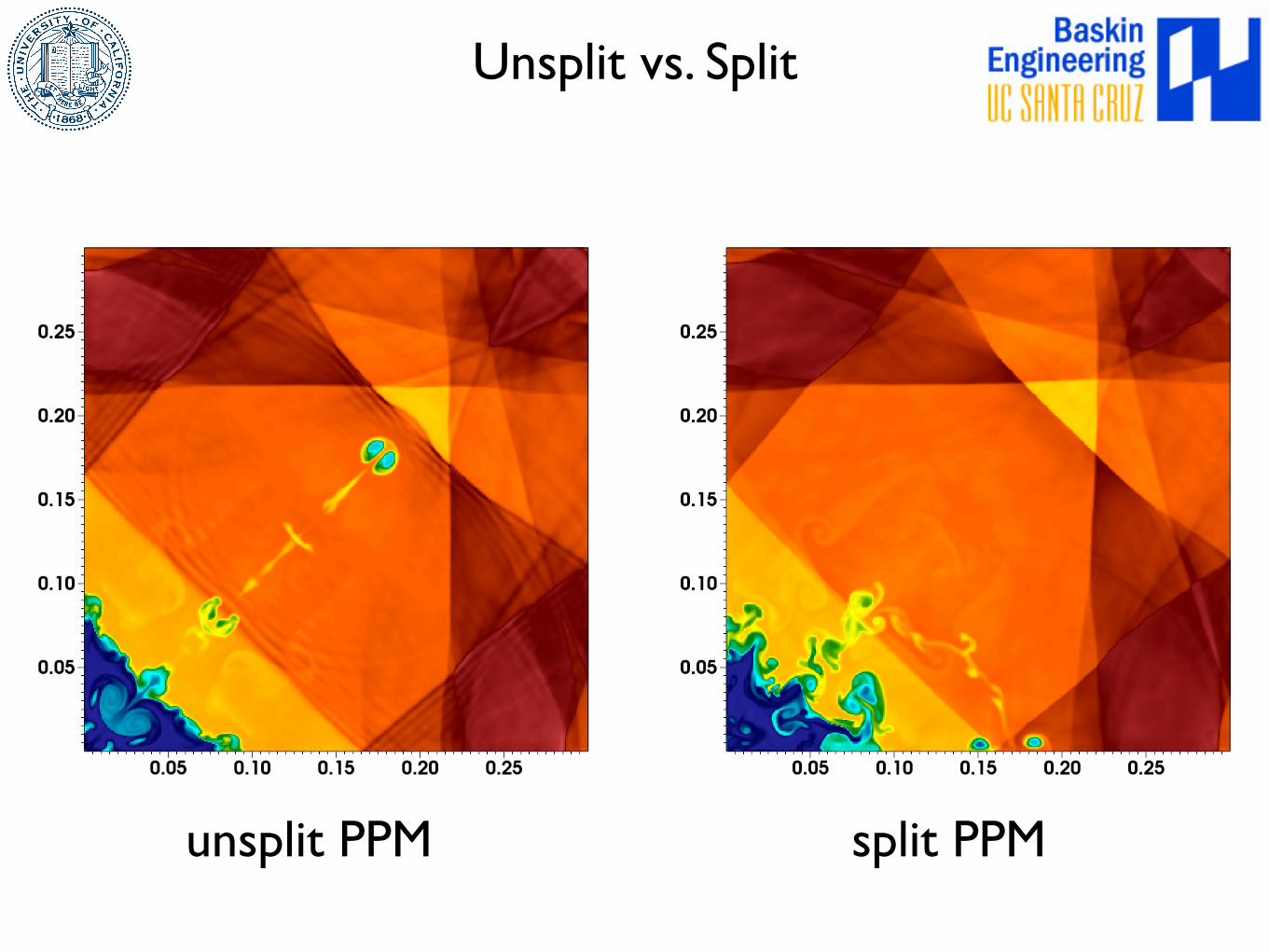
Unsplit vs. Split
unsplit PPM split PPM
Excellent Resources

Last Episode
1. High Performance Computing
2. Ideas on Numerical Methods
3. Validation & Predictive Science

In Collaboration with
U of Chicago: D. Q. Lamb
P. TzeferacosN. Flocke
C. GrazianiK. Weide
U of Oxford:G. GregoriJ. Meinecke
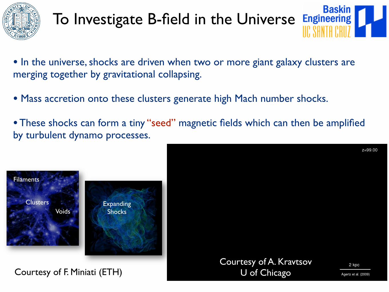
To Investigate B-field in the Universe
• In the universe, shocks are driven when two or more giant galaxy clusters are merging together by gravitational collapsing.
• Mass accretion onto these clusters generate high Mach number shocks.
• These shocks can form a tiny “seed” magnetic fields which can then be amplified by turbulent dynamo processes.
Courtesy of F. Miniati (ETH)
Filaments
ClustersVoids
Expanding Shocks
Courtesy of A. KravtsovU of Chicago
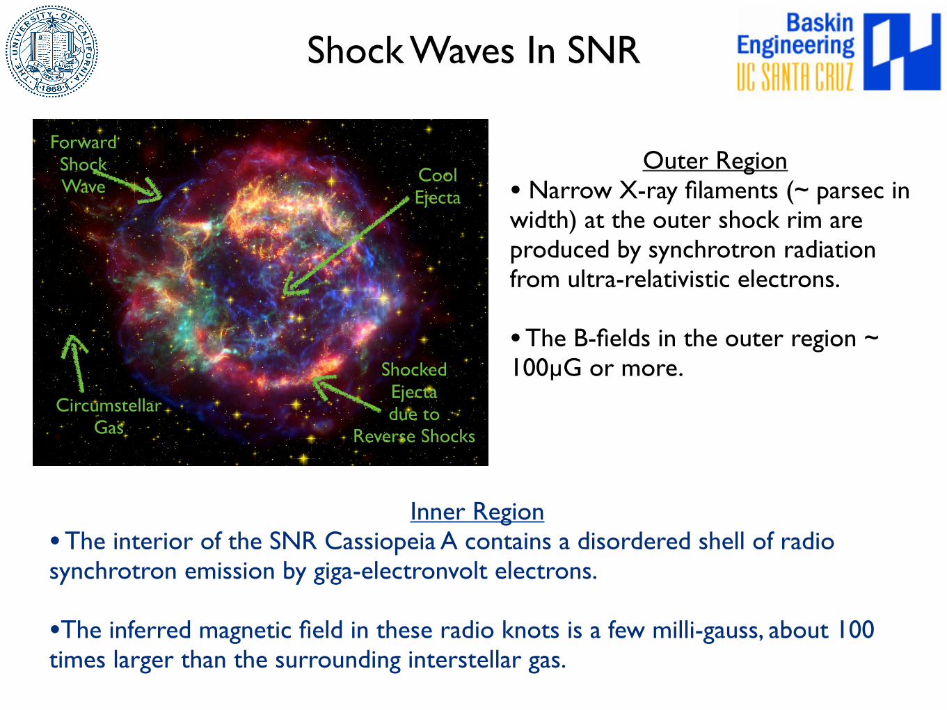
Shock Waves In SNR
Inner Region• The interior of the SNR Cassiopeia A contains a disordered shell of radio synchrotron emission by giga-electronvolt electrons.
•The inferred magnetic field in these radio knots is a few milli-gauss, about 100 times larger than the surrounding interstellar gas.
ForwardShock Wave
ShockedEjectadue to
Reverse Shocks
CircumstellarGas
CoolEjecta
Outer Region• Narrow X-ray filaments (~ parsec in width) at the outer shock rim are produced by synchrotron radiation from ultra-relativistic electrons.
• The B-fields in the outer region ~ 100µG or more.
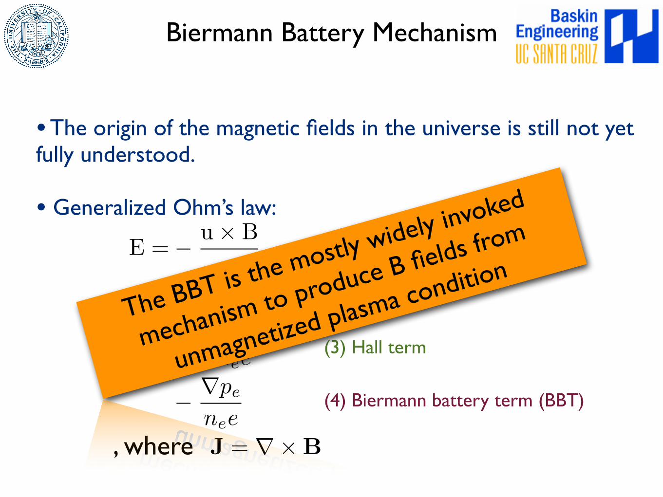
Biermann Battery Mechanism
• The origin of the magnetic fields in the universe is still not yet fully understood. • Generalized Ohm’s law:
J = r⇥B, where
(1) dynamo term
(2) resistive term
(3) Hall term
(4) Biermann battery term (BBT)
E =� u⇥ B
c+ ⌘J
+J⇥ B
cnee
� rpenee
The BBT is the mostly widely invoked
mechanism to produce B fields from
unmagnetized plasma condition
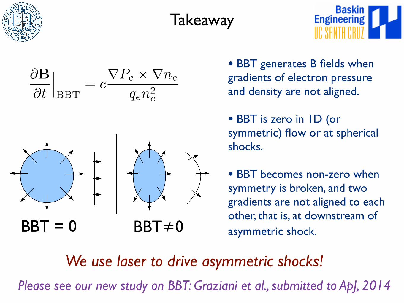
Takeaway
@B
@t
���BBT
= crPe ⇥rne
qen2e
• BBT generates B fields when gradients of electron pressure and density are not aligned.
• BBT is zero in 1D (or symmetric) flow or at spherical shocks.
• BBT becomes non-zero when symmetry is broken, and two gradients are not aligned to each other, that is, at downstream of asymmetric shock. BBT = 0 BBT≠0BBT = 0
We use laser to drive asymmetric shocks! Please see our new study on BBT: Graziani et al., submitted to ApJ, 2014
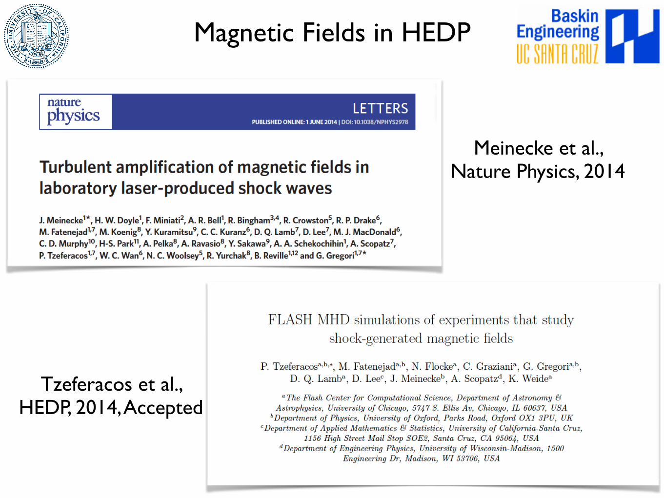
Magnetic Fields in HEDP
Tzeferacos et al., HEDP, 2014, Accepted
Meinecke et al., Nature Physics, 2014
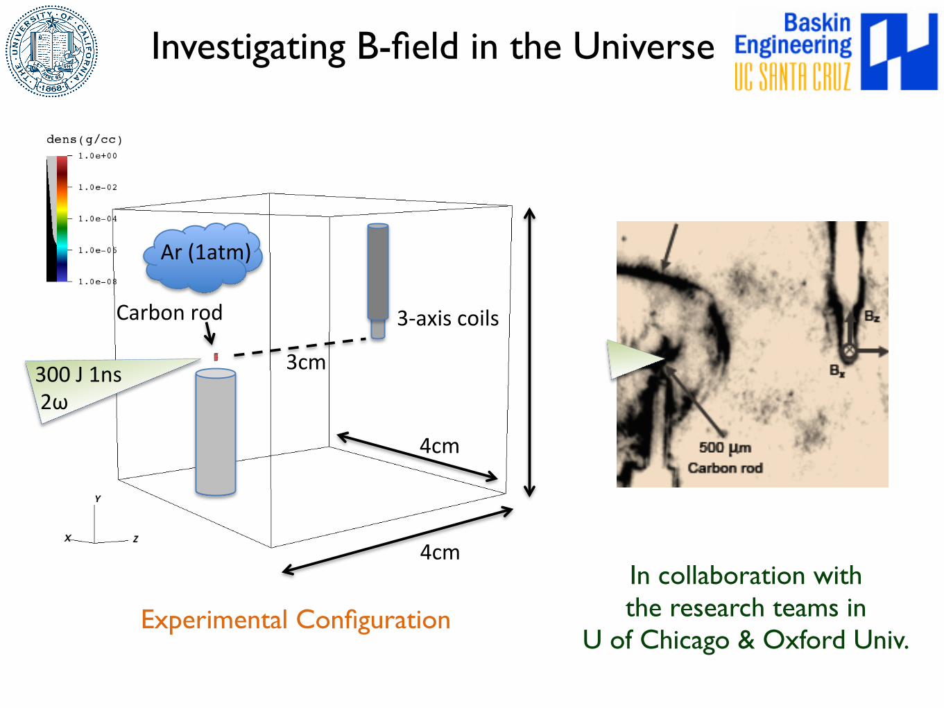
3cm$300$J$1ns$$2ω$
3,axis$coils$
Ar$(1atm)$
4cm$
Carbon$rod$
4cm$
Investigating B-field in the Universe
In collaboration with the research teams in
U of Chicago & Oxford Univ.Experimental Configuration
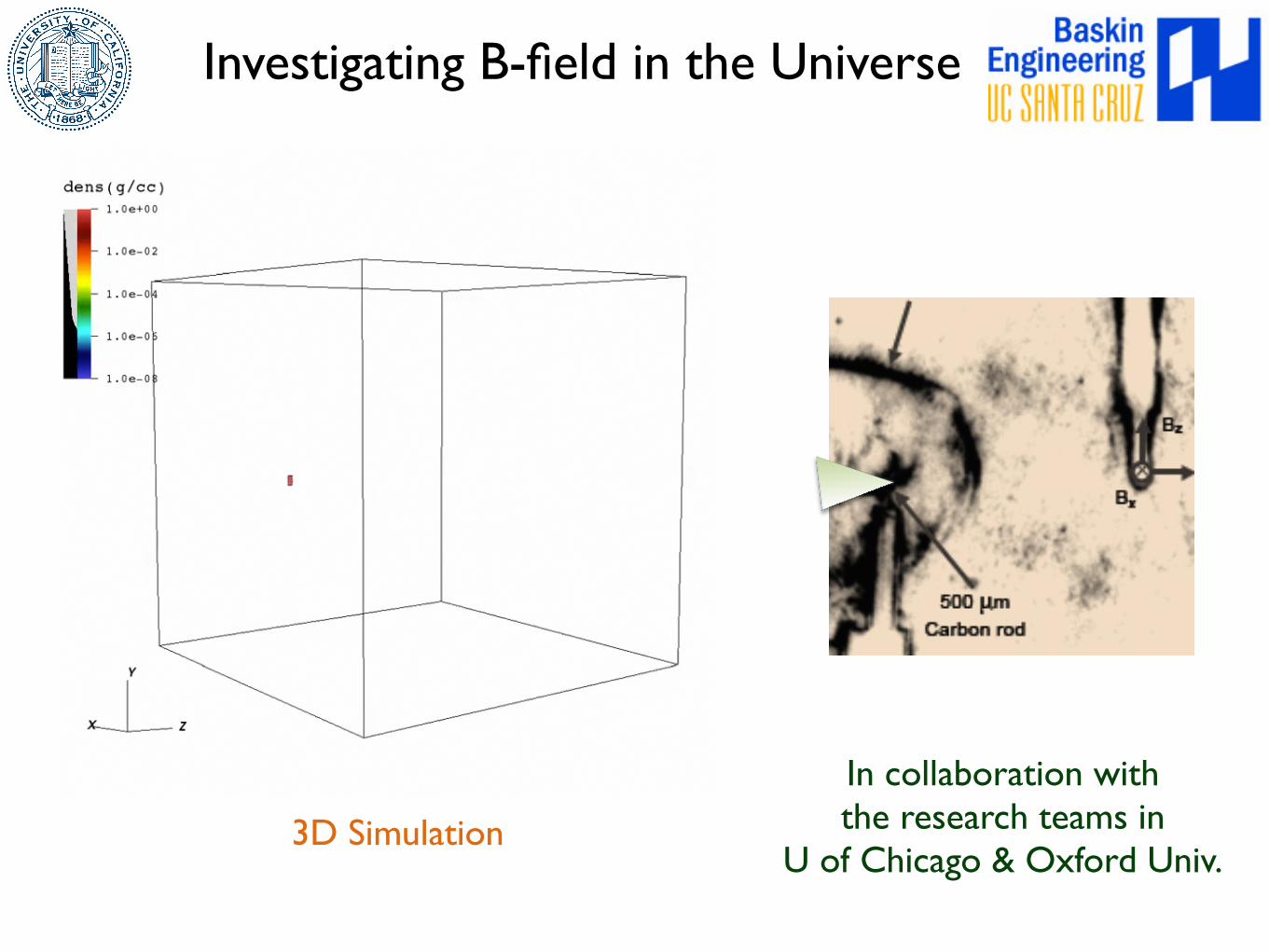
In collaboration with the research teams in
U of Chicago & Oxford Univ.
Investigating B-field in the Universe
3D Simulation
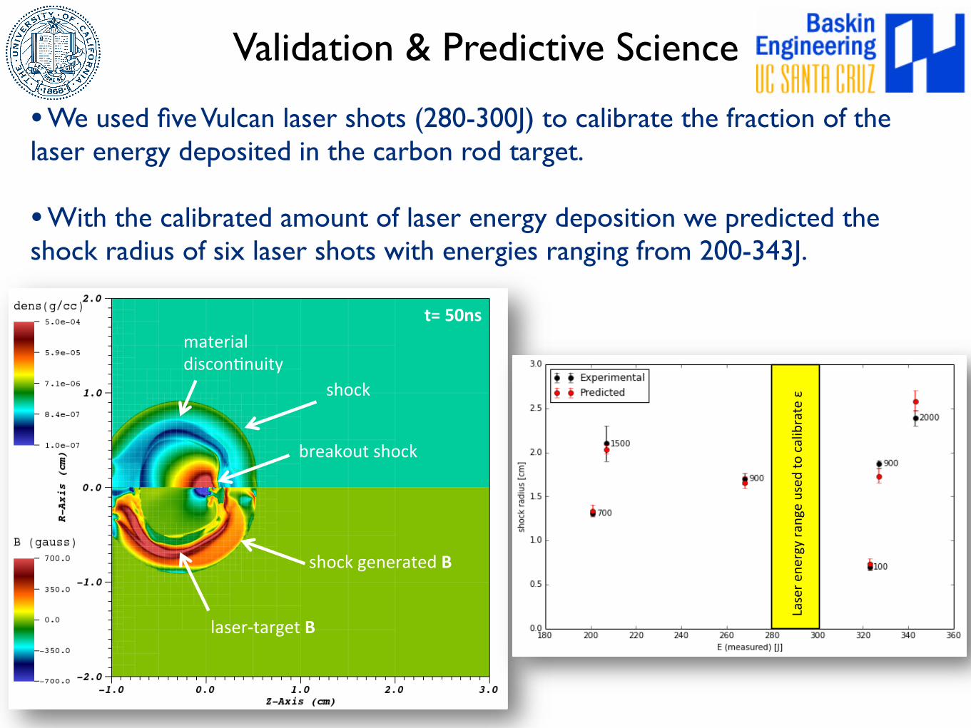
Validation & Predictive Science
breakout)shock)
material)discon2nuity)
shock)
shock)generated)B"
laser5target)B"
t="50ns"
Laser&e
nergy&range&used
&to&calibrate&ε&
• We used five Vulcan laser shots (280-300J) to calibrate the fraction of the laser energy deposited in the carbon rod target.
• With the calibrated amount of laser energy deposition we predicted the shock radius of six laser shots with energies ranging from 200-343J.
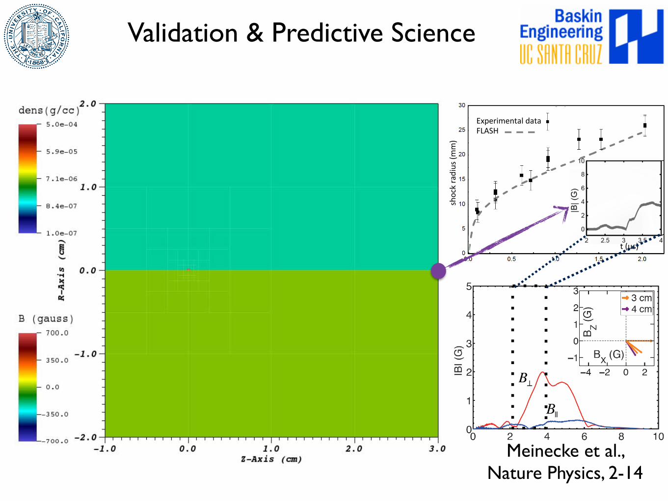
Validation & Predictive Science
Experimental,data,FLASH,
shock,radius,(m
m),
t,(μs),
Meinecke et al., Nature Physics, 2-14
Summary
▪Novel ideas of numerical algorithms can play the key fundamental
role in many areas in modern science.
▪Computational mathematics is one of the corner stone research
areas that can provide major predictive scientific tools.
▪Numerical simulations can help designing better scientific
directions in wide ranges of research applications, especially in
physical science and engineering.

Thanks! Questions?
Dongwook Lee: [email protected]
ams.soe.ucsc.edu/people/dongwook
FLASH: www.flash.uchicago.edu

Supplementary Slides
Relavant Questions
‣ What is scientific computing?
‣ How do we want to use computer for it?
‣ What should we do in order to use computing resources in a better way?
‣ Can numerical algorithms and computational mathematics improve computations?
‣ High-performance computing: petascale (or exascale ?)
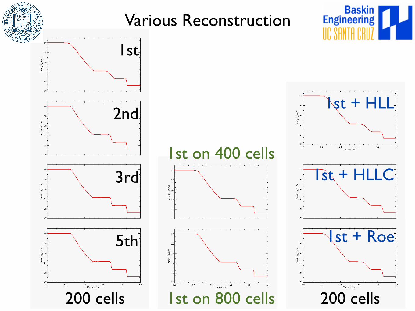
Various Reconstruction
1st
2nd
3rd
5th
200 cells
1st on 400 cells
1st on 800 cells
1st + HLL
200 cells
1st + HLLC
1st + Roe
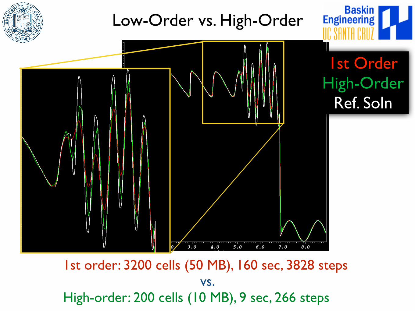
Low-Order vs. High-Order
1st OrderHigh-Order
Ref. Soln
1st order: 3200 cells (50 MB), 160 sec, 3828 stepsvs.
High-order: 200 cells (10 MB), 9 sec, 266 steps