
The endogenous grid method for discrete-continuous dynamic ...
49
Quantitative Economics 8 (2017), 317–365 1759-7331/20170317 The endogenous grid method for discrete-continuous dynamic choice models with (or without) taste shocks Fedor I skhakov Research School of Economics, Australian National University and ARC Centre of Excellence in Population Ageing Research, University of New South Wales Thomas H. J ørgensen Department of Economics, University of Copenhagen J ohn Rust Department of Economics, Georgetown University Bertel Schjerning Department of Economics, University of Copenhagen We present a fast and accurate computational method for solving and estimating a class of dynamic programming models with discrete and continuous choice vari- ables. The solution method we develop for structural estimation extends the en- dogenous grid-point method (EGM) to discrete-continuous (DC) problems. Dis- crete choices can lead to kinks in the value functions and discontinuities in the optimal policy rules, greatly complicating the solution of the model. We show how these problems are ameliorated in the presence of additive choice-specific independent and identically distributed extreme value taste shocks that are typi- cally interpreted as “unobserved state variables” in structural econometric appli- cations, or serve as “random noise” to smooth out kinks in the value functions in numerical applications. We present Monte Carlo experiments that demonstrate the reliability and efficiency of the DC-EGM algorithm and the associated maxi- mum likelihood estimator for structural estimation of a life-cycle model of con- sumption with discrete retirement decisions. Fedor Iskhakov: [email protected] Thomas H. Jørgensen: [email protected] John Rust: [email protected] Bertel Schjerning: [email protected] We acknowledge helpful comments from Chris Carroll, Giulio Fella and many other people, participants at seminars at University of New South Wales, University of Copenhagen, the 2012 conferences of the Society of Economic Dynamics, the Society for Computational Economics, and the Initiative for Computational Economics at Zurich (ZICE 2014, 2015, 2017). This paper is part of the Intelligent road user charging (IRUC) research project financed by the Danish Council for Strategic Research (DSF). Iskhakov, Rust, and Schjern- ing gratefully acknowledge this support. Iskhakov gratefully acknowledges the financial support from the Australian Research Council Centre of Excellence in Population Ageing Research (project CE110001029) and Michael P. Keane’sAustralian Research Council Laureate Fellowship (project FL110100247). Jørgensen gratefully acknowledges financial support from the Danish Council for Independent Research in Social Sci- ences (FSE, Grant 4091-00040). Copyright © 2017 The Authors. Quantitative Economics. The Econometric Society. Licensed under the Creative Commons Attribution-NonCommercial License 4.0. Available at http://www.qeconomics.org. DOI: 10.3982/QE643
Transcript of The endogenous grid method for discrete-continuous dynamic ...

Quantitative Economics 8 (2017), 317–365 1759-7331/20170317
The endogenous grid method for discrete-continuous dynamicchoice models with (or without) taste shocks
Fedor IskhakovResearch School of Economics, Australian National University and ARC Centre of Excellence
in Population Ageing Research, University of New South Wales
Thomas H. JørgensenDepartment of Economics, University of Copenhagen
John RustDepartment of Economics, Georgetown University
Bertel SchjerningDepartment of Economics, University of Copenhagen
We present a fast and accurate computational method for solving and estimating aclass of dynamic programming models with discrete and continuous choice vari-ables. The solution method we develop for structural estimation extends the en-dogenous grid-point method (EGM) to discrete-continuous (DC) problems. Dis-crete choices can lead to kinks in the value functions and discontinuities in theoptimal policy rules, greatly complicating the solution of the model. We showhow these problems are ameliorated in the presence of additive choice-specificindependent and identically distributed extreme value taste shocks that are typi-cally interpreted as “unobserved state variables” in structural econometric appli-cations, or serve as “random noise” to smooth out kinks in the value functions innumerical applications. We present Monte Carlo experiments that demonstratethe reliability and efficiency of the DC-EGM algorithm and the associated maxi-mum likelihood estimator for structural estimation of a life-cycle model of con-sumption with discrete retirement decisions.
Fedor Iskhakov: [email protected] H. Jørgensen: [email protected] Rust: [email protected] Schjerning: [email protected] acknowledge helpful comments from Chris Carroll, Giulio Fella and many other people, participants atseminars at University of New South Wales, University of Copenhagen, the 2012 conferences of the Societyof Economic Dynamics, the Society for Computational Economics, and the Initiative for ComputationalEconomics at Zurich (ZICE 2014, 2015, 2017). This paper is part of the Intelligent road user charging (IRUC)research project financed by the Danish Council for Strategic Research (DSF). Iskhakov, Rust, and Schjern-ing gratefully acknowledge this support. Iskhakov gratefully acknowledges the financial support from theAustralian Research Council Centre of Excellence in Population Ageing Research (project CE110001029)and Michael P. Keane’s Australian Research Council Laureate Fellowship (project FL110100247). Jørgensengratefully acknowledges financial support from the Danish Council for Independent Research in Social Sci-ences (FSE, Grant 4091-00040).
Copyright © 2017 The Authors. Quantitative Economics. The Econometric Society. Licensed under theCreative Commons Attribution-NonCommercial License 4.0. Available at http://www.qeconomics.org.DOI: 10.3982/QE643
318 Iskhakov, Jørgensen, Rust, and Schjerning Quantitative Economics 8 (2017)
Keywords. Life-cycle model, discrete and continuous choice, Bellman equation,Euler equation, retirement choice, endogenous grid-point method, nested fixedpoint algorithm, extreme value taste shocks, smoothed max function, structuralestimation.
JEL classification. C13, C63, D91.
1. Introduction
This paper develops a fast new solution algorithm for structural estimation of dynamicprogramming models with discrete and continuous choices. The algorithm we proposeextends the endogenous grid method (EGM) by Carroll (2006) to discrete-continuous(DC) models. We refer to it as the DC-EGM algorithm. We embed the DC-EGM algo-rithm in the inner loop of the nested fixed point (NFXP) algorithm (Rust (1987)), andshow that the resulting maximum likelihood estimator produces accurate estimates ofthe structural parameters at low computational cost.
There is an extensive literature on static models of discrete/continuous choice:a classic example is Dubin and McFadden (1984). However, the focus of our paper ison dynamic DC models. A classic example is the life-cycle model with discrete retire-ment and continuous consumption decisions. While there is a well developed literatureon solution and estimation of dynamic discrete choice models, and a separate literatureon estimation of life-cycle models without discrete choices, there has been far less workon solution and estimation of DC models.1
There is good reason why DC models are much less commonly seen in the literature:they are substantially harder to solve. The value functions of models with only continu-ous choices are typically concave and the optimal policy function can be found from theEuler equation. EGM avoids the need to numerically solve the nonlinear Euler equationfor the optimal continuous choice at each grid point in the state space. Instead, EGMspecifies an exogenous grid over an endogenous quantity (e.g., savings) to analyticallycalculate the optimal policy rule (e.g., consumption) and endogenously determine thepredecision state (e.g., beginning-of-period resources).2 DC-EGM retains the main de-sirable properties of EGM, namely it avoids the bulk of costly root-finding operationsand handles borrowing constraints in an efficient manner.
Dynamic programs that have only discrete choices are substantially easier to solve,since the optimal decision rule is simply the alternative with the highest choice-specific
1There are relatively few examples of structural estimation or numerical solution of DC models. Someprominent examples include the model of optimal nondurable consumption and housing purchases(Carroll and Dunn (1997)), optimal saving and retirement (French and Jones (2011)), and optimal saving,labor supply, and fertility (Adda, Dustmann, and Stevens (2017)).
2The EGM is in fact a specific application of what is referred to as “controlling the postdecision state”in operations research and engineering (Bertsekas, Lee, van Roy, and Tsitsiklis (1997)). Carroll (2006) in-troduced the idea in economics by developing the EGM algorithm with the application to the buffer-stockprecautionary savings model. Since then the idea became widespread in economics. Further generaliza-tions of EGM include Barillas and Fernández-Villaverde (2007), Hintermaier and Koeniger (2010), Ludwigand Schön (2013), Fella (2014), Iskhakov (2015). Jørgensen (2013) compares the performance of EGM tomathematical programming with equilibrium constraints (MPEC).

Quantitative Economics 8 (2017) DC-EGM method for dynamic choice models 319
value. However, solving dynamic programming problems that combine continuous anddiscrete choices is substantially more complicated, since discrete choices introducekinks and nonconcave regions in the value function that lead to discontinuities in thepolicy function of the continuous choice (consumption). This can lead to situationswhere the Euler equation has multiple solutions for consumption, and hence it is only anecessary rather than a sufficient condition for the optimal consumption rule (Clausenand Strub (2013)). This inherent feature of DC problems complicates any method onemight consider for solving DC models.
We illustrate how DC-EGM can deal with these inherent complications using a life-cycle model with a continuous consumption and binary retirement choice with andwithout taste shocks. Our example is a simple extension of the classic life-cycle modelof Phelps (1962) where, in the absence of a retirement decision, the optimal consump-tion rule could hardly be any simpler—a linear function of resources. However, oncethe discrete retirement decision is added to the consumption–savings problem—in ourcase allowing a worker with logarithmic utility to also make a binary irreversible retire-ment decision—the consumption function becomes unexpectedly complex, with mul-tiple discontinuities in the optimal consumption rule. We derive an analytic solution forthis model and use it to demonstrate the accuracy of the solution obtained numericallyby DC-EGM. We then show how DC-EGM can be used to solve DC models with tasteshocks and investigate its performance as a nested solution method for structural esti-mation of a DP model of retirement.
Fella (2014) showed how the EGM could be adapted to solve nonconcave problems,including models with discrete and continuous choices. In this paper we focus on dis-crete choices and show that introducing independent and identically distributed (i.i.d.)extreme value type I choice-specific taste shocks not only facilitates maximum likeli-hood estimation, but also smooths out some of the kinks in the value functions, therebysimplifying the numerical solution of the model. This approach results in multinomiallogit formulas for the conditional choice probabilities for the discrete choices and aclosed-form expression for the expectation of the value function with respect to thesetaste shocks.3
In econometric applications continuously distributed taste shocks are essential forgenerating predictions from dynamic programming models that are statistically nonde-generate. Such predictions assign a positive (however small) choice probability to everyalternative, and therefore preclude zero likelihood observations. These shocks are in-terpreted as unobserved state variables, that is, idiosyncratic shocks observed by agentsbut not by the econometrician. However, in numerical or theoretical applications, tasteshocks can serve as a smoothing device (homotopy perturbation) that facilitates the nu-merical solution of more advanced DC models that may have excessively many kinksand discontinuities, for example, caused by a large number of discrete choices.
3In principle, the extreme value assumption could be relaxed to allow for other distributions at the costof numerical approximation of choice probabilities and the conditional expectation of the value function.For example, Bound, Stinebrickner, and Waidmann (2010) assume that the discrete choice-specific tasteshocks are Normal rather than extreme value. Yet, we follow the long tradition of discrete choice modelingdating back to McFadden (1973) and Rust (1987).

320 Iskhakov, Jørgensen, Rust, and Schjerning Quantitative Economics 8 (2017)
The inclusion of extreme value type I taste shocks has a long history in discretechoice modeling dating back to the seminal work by McFadden (1973). This assumptionis typically invoked in microeconometric analyses of dynamic discrete choice modelswhere numerical performance boosted by closed-form choice probabilities is particu-larly important; see, for example, Rust (1994) and the recent survey by Aguirregabiriaand Mira (2010). Some recent studies of DC models with extreme value taste shocks in-clude Casanova (2010), Ejrnæs and Jørgensen (2016), Iskhakov and Keane (2016), Oswald(2016), and Adda, Dustmann, and Stevens (2017).
At first glance, the addition of stochastic shocks would appear to make the prob-lem harder to solve, since both the optimal discrete and continuous decision rules willnecessarily be functions of these stochastic shocks. However, we show that a variety ofstochastic variables in DC models smooth out many of the kinks in the value functionsand the discontinuities in the optimal consumption rules. In the absence of smooth-ing, we show that every kink induced by the comparison of the discrete choice-specificvalue functions in any period t propagates backward in time to all previous periods as amanifestation of the decision maker’s anticipation of the future discrete action. The re-sulting accumulation of kinks during backward induction presents the most significantchallenge for the numerical solution of DC models. In the presence of taste shocks thedecision maker can only anticipate a particular future discrete action to be more or lessprobable, and thus the primary reason for the accumulation of kinks disappears. Thus,the combination of taste shocks and the stochastic variables in the model is perhaps themost powerful device to prevent the propagation and accumulation of kinks.4
In the case where extreme value taste shocks are used as a logit smoothing device ofan underlying deterministic model of interest, we show that the latter problem can beapproximated by the smoothed model to any desirable degree of precision. The scaleparameter σ ≥ 0 of the corresponding extreme value distribution then serves as a ho-motopy or smoothing parameter. When σ is sufficiently large, the nonconcave regionsnear the kinks in the nonsmoothed value function disappear and the value functionsbecome globally concave. But even small values of σ smooth out many of the kinks inthe value functions and suppress their accumulation in the process of backward induc-tion as noted above. An additional benefit of the taste shocks is that standard integrationmethods, such as quadrature rules, apply when the expected value function is a smoothfunction.
We run a series of Monte Carlo simulations to investigate the performance of DC-EGM for structural estimation of the life-cycle model with the discrete retirement deci-sion. We find that a maximum likelihood estimator that nests the DC-EGM algorithmperforms well. It quickly produces accurate estimates of the structural parameters ofthe model even when fairly coarse grids over wealth are used. We find the cost of “over-smoothing” to be negligible in the sense that the parameter estimates of a perturbedmodel with stochastic taste shocks are estimated very accurately even if the true modeldoes not have taste shocks. Thus, even in the case where the addition of taste shocks
4Contrary to the macro literature that uses stochastic elements such as employment lotteries (Rogerson(1988), Prescott (2005), Ljungqvist and Sargent (2005)) to smooth out nonconvexities, the taste shock weintroduce in DC models in general do not fully convexify the problem.

Quantitative Economics 8 (2017) DC-EGM method for dynamic choice models 321
results in a misspecification of the model, the presence of these shocks improves theaccuracy of the solution and reduces computation time without increasing the approxi-mation bias significantly. Even when very few grid points are used to solve the model, wefind that smoothing the problem improves the root mean square error (RMSE). Partic-ularly, with an appropriate degree of smoothing (σ), we can reduce the number of gridpoints by an order of magnitude without much increase in the RMSE of the parameterestimates.
DC-EGM is applicable to many fields of economics and has been implementedin several recent empirical applications. Ameriks, Briggs, Caplin, Shapiro, and Tonetti(2015) study how the need for long term care and bequest motive interact withgovernment-provided support to shape the wealth profile of the elderly. They use anendogenous grid method similar to DC-EGM to solve and estimate the correspond-ing nonconcave model. Iskhakov and Keane (2016) employ DC-EGM to estimate a life-cycle model of discrete labor supply, human capital accumulation, and savings for theAustralian population. They use the model to evaluate Australia’s defined contributionpension scheme with means-tested minimal pension, and quantify the effects of antici-pated and unanticipated policy changes. Yao, Fagereng, and Natvik (2015) use DC-EGMto analyze how housing and mortgage debt affects consumers’ marginal propensity toconsume. They estimate a model in which households hold debt, financial assets, andilliquid housing, and find that a substantial fraction of households are likely to behavein a “hand-to-mouth” fashion despite having significant wealth holdings. Druedahl andJørgensen (2015) employ a modified version of DC-EGM to analyze the credit card debtpuzzle. They solve a model of optimal consumption and debt holdings, and show how,for some parameterizations of the model, a large group of consumers find it optimalto simultaneously hold positive gross debt and positive gross assets even though theinterest rate on the debt is much higher than the rate on the assets. Ejrnæs and Jør-gensen (2016) use DC-EGM to estimate a model of optimal consumption and savingwith a fertility choice to analyze the saving behavior around intended and unintendedchild births. They model the fertility process as a discrete choice over effort to conceivea child subject to a biological fecundity constraint and allow for the possibility of unin-tended child births through imperfect contraceptive control.
In the next section we present a simple extension of the life-cycle model of consump-tion and savings with logarithmic utility studied by Phelps (1962) and Deaton (1991)where we allow for a discrete retirement decision. We derive a closed-form solution tothis problem and discuss its properties. Using this simple model we demonstrate the ac-curacy of the deterministic version of DC-EGM. We then introduce extreme value tasteshocks and show how the implied smoothing affects the value functions and the optimalpolicy rules. In particular, we show that the error introduced by “extreme value smooth-ing” is uniformly bounded, and prove that the solution of the smoothed DP problemwith taste shocks converges to the solution to the DP problem without taste shocks asthe scale of the shocks approaches zero. Section 3 presents the full DC-EGM algorithm.In Section 4 we show how it is incorporated in the nested fixed point algorithm for max-imum likelihood estimation of the structural parameters in the retirement model. We

322 Iskhakov, Jørgensen, Rust, and Schjerning Quantitative Economics 8 (2017)
present the results of a series of Monte Carlo experiments in which we explore the per-formance of the estimator in a variety of settings. We conclude with a short discussionof the range of models that DC-EGM is applicable to and discuss some open issues withthis method.
2. An illustrative problem: Consumption and retirement
This section extends the classic life-cycle consumption–savings model of Phelps (1962)and Deaton (1991) to allow for a discrete retirement decision. We derive an analytic so-lution to this problem with logarithmic utility to both illustrate the complexity causedby the addition of a discrete retirement choice and show how DC-EGM computes thissolution. While we focus on this simple example for expositional clarity, DC-EGM can beapplied to a much more general class of problems that include taste and income shocks.We will discuss these extensions in Section 3 and show how the addition of shocks canactually simplify the solution of the model using DC-EGM.
2.1 Deterministic model of consumption–savings and retirement
Consider the discrete-continuous (DC) dynamic optimization problem
max{ct �dt }Tt=1
T∑t=1
βt(log(ct)− δdt
)(1)
involving choices of consumption ct and whether to retire dt , to maximize lifetime dis-counted utility. Let dt = 0 denote retirement, let dt = 1 denote continued work, and letδ > 0 be the disutility of work. To simplify the exposition, we assume retirement is ab-sorbing, that is, a retiree cannot return to work.5
We solve (1) subject to a sequence of period-specific borrowing constraints, ct ≤Mt ,where Mt = R(Mt−1 − ct−1)+ ydt−1 is the consumer’s consumable resources (wealth) atthe beginning of period t. There is a fixed, nonstochastic gross interest rate R and laborincome y for workers. The continuous consumption decision and discrete retirementdecision are made at the start of each period, whereas interest earnings and labor in-come are paid at the end of the period.6
Let Vt(M) and Wt(M) be the expected discounted lifetime utility of a worker and aretiree, respectively, in period t of their life. The choice problem of the worker can beexpressed recursively through the Bellman equation as
Vt(M)= max{vt(M�0)� vt(M�1)
}� (2)
5This allows us to focus primarily on the worker’s problem. In the absence of absorbing retirement, theretiree’s problem involves a discrete choice (returning to work or staying retired), and can be solved by DC-EGM similarly to the worker’s problem.
6This timing convention is standard in the literature and it removes the need to include income as aseperate state variable when we extend this model to a much wider class of problems with stochastic R
and/or y .

Quantitative Economics 8 (2017) DC-EGM method for dynamic choice models 323
where the choice-specific value functions vt(M�d), d ∈ {0�1}, are given by
vt(M�0)= max0≤c≤M
{log(c)+βWt+1
(R(M − c)
)}� (3)
vt(M�1)= max0≤c≤M
{log(c)− δ+βVt+1
(R(M − c)+ y
)}� (4)
The Bellman equation for the retiree’s problem, which does not involve a discrete choice,is much simpler and can be written as
Wt(M)= max0≤c≤M
{log(c)+βWt+1
(R(M − c)
)}� (5)
The value function for a retiree Wt(M) has a closed-form solution given by Phelps(1962, p. 742), so we focus on solving the worker’s problem, that is, solving for the valuefunction Vt(M) and the optimal consumption rule ct(M). The fact that the future looksthe same from the point of view of the retiree and from the point of view of the workerwho decides to retire, can be verified from the fact that the right hand side of (3) is iden-tical to that of (5). Therefore, we have Wt(M) = vt(M�0), and the consumption functionof the retiree is identical to the choice-specific consumption function of the worker whodecided to retire, ct(M�0), where the second argument denotes the retirement choice.
Note that even if vt(M�0) and vt(M�1) are concave functions of M , the value func-tion Vt(M) is the maximum of these two concave functions by (2) and will generally notbe globally concave (Clausen and Strub (2013)). Further, Vt(M) will generally have a kinkpoint at the value M = Mt where the two choice-specific value functions cross, that is,vt(Mt�1) = vt(Mt�0). We refer to these as primary kinks because they constitute opti-mal retirement thresholds for the worker in each period t. The optimal retirement rule isgiven by dt(M) = 1 if M <Mt and dt(M) = 0 if M ≥Mt .
The worker is indifferent between retiring and working at the primary kink Mt , andVt(M) is nondifferentiable at this point. However, the left and right hand side derivatives,V −t (M) and V +
t (M), exist and satisfy V −t (Mt) < V +
t (Mt). The discontinuity in the deriva-tive of Vt(M) at Mt leads to a discontinuity in the optimal consumption function in theprevious period t − 1 because the Bellman equation for Vt−1(M) depends on Vt(M). Inturn, this causes a kink in Vt−1(M) that we label a secondary kink since it is a reflection ofthe primary kink in Vt(M). Thus, the primary kinks propagate back in time and manifestthemselves in an accumulation of secondary kinks in the value functions in earlier peri-ods, resulting in an increasing number of discontinuities in the consumption functionsin earlier periods of the life cycle. The discontinuities in consumption rules in period t
are caused by the worker’s anticipation of landing exactly at the kink points in periodst + 1� t + 2� � � � �T under the optimal consumption policy.
Theorem 1 (Analytical Solution to the Retirement Problem). Assume that income anddisutility of work are time-invariant, the discount factor β and the disutility of work δ arenot too large, that is,
βR≤ 1 and δ < (1 +β) log(1 +β)� (6)

324 Iskhakov, Jørgensen, Rust, and Schjerning Quantitative Economics 8 (2017)
and instantaneous utility is given by u(c) = log(c). Then for τ ∈ {1� � � � �T } the optimalconsumption rule in the worker’s problem (2)–(4) is given by
cT−τ(M)=
⎧⎪⎪⎪⎪⎪⎪⎪⎪⎪⎪⎪⎪⎪⎪⎪⎪⎪⎪⎪⎪⎪⎪⎪⎪⎪⎪⎪⎪⎪⎪⎪⎪⎪⎪⎪⎪⎪⎪⎪⎪⎪⎪⎨⎪⎪⎪⎪⎪⎪⎪⎪⎪⎪⎪⎪⎪⎪⎪⎪⎪⎪⎪⎪⎪⎪⎪⎪⎪⎪⎪⎪⎪⎪⎪⎪⎪⎪⎪⎪⎪⎪⎪⎪⎪⎪⎩
M if M ≤ y/Rβ�
[M + y/R]/(1 +β) if y/Rβ ≤M ≤Ml1T−τ�[
M + y(1/R+ 1/R2)]/(1 +β+β2) if M
l1T−τ ≤M ≤ M
l2T−τ�
· · · · · ·[M + y
(τ−1∑i=1
R−i
)](τ−1∑i=0
βi
)−1
if Mlτ−2T−τ ≤M ≤ M
lτ−1T−τ�[
M + y
(τ∑
i=1
R−i
)](τ∑
i=0
βi
)−1
if Mlτ−1T−τ ≤M <M
rτ−1T−τ�[
M + y
(τ−1∑i=1
R−i
)](τ∑
i=0
βi
)−1
if Mrτ−1T−τ ≤M <M
rτ−2T−τ�
· · · · · ·[M + y
(1/R+ 1/R2)]( τ∑
i=0
βi
)−1
if Mr2T−τ ≤M <M
r1T−τ�
[M + y/R](
τ∑i=0
βi
)−1
if Mr1T−τ ≤M <MT−τ�
M
(τ∑
i=0
βi
)−1
if M ≥MT−τ�
(7)
The segment boundaries are totally ordered with
y/Rβ<Ml1T−τ < · · · <M
lτ−1T−τ <M
rτ−1T−τ < · · · <M
r1T−τ <MT−τ� (8)
and the rightmost threshold MT−τ, given by
MT−τ = (y/R)e−K
1 − e−K� where K = δ
(τ∑
i=0
βi
)−1
� (9)
defines the smallest level of wealth sufficient to induce the consumer to retire at age t =T − τ.
The proof of Theorem 1—in particular, the expressions for the kink points MliT−τ and
MriT−τ—is available in a supplementary file on the journal website, http://qeconomics.
org/supp/643/supplement.pdf. However, we show how this solution is derived when weintroduce the DC-EGM algorithm in the next section.7
7Note that the assumptions on the parameters β, δ, and R are needed to ensure the ordering of thebounderies (8). Modified versions of Theorem 1 hold under weaker conditions, including a version whereincome and the disutility of work are age-dependent. However, depending on the paths of income and

Quantitative Economics 8 (2017) DC-EGM method for dynamic choice models 325
Theorem 1 establishes that the optimal consumption rule of the worker cT−τ(M) ispiecewise linear in M , and in period t consists of 2(T − t)+1 segments. The first segmentwhere M < y/Rβ is the credit constrained region where the agent consumes all availablewealth and does not save. The next T − t − 1 segments are demarcated by the liquidity
constraint kink points Mljt that define values of M at which the consumer is liquidity
constrained at age t + j but not at any earlier age. The remaining segments are definedby the secondary kinks, M
rjt , j = 1� � � � �T − t − 1, and represent the largest level of saving
for which it is optimal to retire at age t + j but not at any earlier age. Finally, Mt is theretirement threshold, which denotes the minimum level of wealth that is required toretire. This is also the primary kink point as explained above. The optimal consumptionfunction is discontinuous at points M
rjt , and Mt , so in total there are T − t downward
jumps in the consumption function.Theorem 1 implies that the value function Vt(M) is piecewise logarithmic with the
same kink points, and can be written as Vt(M) = Bt log(ct(M))+Ct for constants (Bt�Ct)
that depend on the region that M falls into. The function Vt(M) has one primary kink atthe optimal retirement threshold Mt and T − t − 1 secondary kinks at M
rjt , j = 1� � � � �T −
t − 1. In addition there are T − t kinks related to current and future liquidity constraints
at M = y/Rβ and Mljt , j = 1� � � � �T − t − 1. If Rβ = 1, the liquidity-related kink points
collapse to a single point M = y/Rβ = y = Ml1t = · · · = M
lT−t−1t , as in the case shown in
Figure 3 in Section 2.3.
2.2 DC-EGM for problems without taste shocks
We are now in a position to introduce a generalization of the EGM algorithm for solv-ing discrete-continuous problems that we call the DC-EGM algorithm. We describe DC-EGM by showing how it can be used to solve for the optimal consumption rule in thelast three periods of the worker’s problem. As the original EGM constitutes a buildingblock of DC-EGM, we illustrate it as well using the consumption choice problem of theretiree. After explaining the DC-EGM algorithm, we compare its numerical performanceand show that DC-EGM can closely approximate the analytic solution in Theorem 1.
DC-EGM is a backward induction algorithm that uses the inverted Euler equation tosequentially compute (potentially without root-finding) the choice-specific value func-tions vt(M�d) and the corresponding choice-specific consumption functions ct(M�d)
starting at the last period of life, T . Note that in a generic period t of the backward induc-tion, the Bellman equation (4) of a worker who remains working implies the followingfirst order condition for the consumption choice known as the Euler equation:
0 = u′(c)−βRu′(ct+1(R(M − c)+ y
))= 1/c − βR
ct+1(R(M − c)+ y)�
(10)
disutility of work, some of the intermediate thresholds in Theorem 1 may not exist or may be equal to eachother.

326 Iskhakov, Jørgensen, Rust, and Schjerning Quantitative Economics 8 (2017)
Similarly the Bellman equation (3) for the worker who decides to retire implies the Eulerequation
0 = u′(c)−βRu′(crt+1(R(M − c)
))= 1/c − βR
crt+1(R(M − c))�
(11)
where the second equality shows the case of u(c) = log(c). Given the period t + 1 opti-mal consumption functions ct+1(M) for workers and crt+1(M) for retirees, the solutionsto these Euler equations yield the period t choice-specific consumption functions of theworker, ct(M�d).8 The solutions are computed by applying the inverse of the marginalutility to the second component in (10) and (11). When such an inverse function is an-alytical, specifying an exogenous grid over end-of-period saving A = M − c facilitatessolving for optimal current consumption in closed form without resorting to iterativenumerical methods. This is the idea behind the endogenous grid method (EGM) pro-posed by Carroll (2006) that we build on.
Consider the terminal period T . The optimal consumption rule is to consume allavailable wealth and, thus, is given by cT (M�d)=M . With positive disutility of working,all agents retire (i.e., MT = 0) since income is paid at the end of the period, so it followsthat dT (M)= 0. This solution provides the base for backward induction.
Now consider a retiree in period T − 1. Note that because the Bellman equation ofthe retiree (5) is identical to that of the worker who decides to retire (3), the Euler equa-tion (11) also characterizes the optimal consumption choices of the retiree, cRt (M). InT − 1 the closed-form solution of (11) is cRT−1(M) = M/(1 + β). Consider how this so-lution is computed using the original EGM algorithm by Carroll (2006). EGM uses theEuler equation (11) to construct an endogenous grid over M from an exogenous grid oversavings A = M − c. Let �A = {A1� � � � �AJ} denote the exogenous grid over savings. Be-cause savings is a sufficient statistic, that is, carries all the information about wealth andconsumption in the period, Euler equation (11) can be solved for c for each point Aj .As mentioned above, when u′(c) is analytically invertible, the solution is also analytical.For the case u(c) = log(c), the solution is easily seen to be crT−1(Mj�T−1) = Aj/β, where
Mj�T−1 is an element of the endogenous grid �MT−1 implied by the exogenous grid oversavings �A in period T − 1. We have Mj�T−1 = Aj + crT−1(Mj�T−1) = Aj(1 + 1/β), whichimplies the EGM solution crT−1(Mj�T−1)= Mj�T−1/(1 +β).
Thus, at the points of the endogenous grid �Mt , EGM produces an exact solution inthe sense that the Euler residuals exactly equal zero. Between these points calculationof the optimal consumption requires function approximation, typically linear interpo-lation. With the latter, EGM produces the exact (linear) solution for the consumptionfunction of a retiree.
8Note the distinction between crt+1(M) and ct+1(M) which are the state-specific optimal consumptionfunctions at time t + 1, and ct(M�0) and ct(M�1) which are the decision-specific consumption functions attime t for the worker. The distinction can be confusing since “work” and “retirement” are both states anddecisions but it is important. We focus on the worker problem and skip the Euler equation for the retireewho have no additional discrete choice over retirement due to our assumption that retirement is absorbing.

Quantitative Economics 8 (2017) DC-EGM method for dynamic choice models 327
Now consider a worker in period T − 1. The worker must solve for two consumptionfunctions cT−1(M�0) and cT−1(M�1) corresponding to the decision to retire or not, re-spectively. However no special complications are created at this point: we simply apply“standard EGM” to solve for the optimal consumption rule of a worker cT−1(M�d) foreach of the discrete decisions d, using Euler equation (10) or (11) just as we describedfor the case of a retiree above. Similar to above, with linear interpolation this also resultsin exact solutions cT−1(M�1) = (M + y/R)/(1 +β) and cT−1(M�0)=M/(1 +β).
To ensure that the credit constraint cT−1 ≤ M is satisfied in the presence of noncap-ital income y, standard EGM has an additional step.9 Namely, from (10) it follows thatinvoking the EGM algorithm with zero savings, Aj = 0, produces an endogenous pointMj�T−1 = y/Rβ. As we show below in Theorem 2, it holds that savings as a function ofwealth must be nondecreasing, and, therefore, for M ≤ y/Rβ the savings must remainzero, that is, cT−1(M�1)= M . To add this additional “credit-constrained” segment to theoptimal consumption function, it is sufficient to add a point M0�T−1 = 0 to the endoge-nous grid �MT−1, and set the corresponding optimal consumption cT−1(M0�T−1�1) =M0�T−1 = 0. This way, when linear interpolation is used, EGM finds the first two seg-ments of the true solution cT−1(M�1) given in equation (7) of Theorem 1 exactly, includ-ing the location of the first kink point.
In summary, when there are discrete choices, DC-EGM invokes the EGM algo-rithm to calculate, via simple linear interpolation as described above, piecewise lin-ear approximations of the decision-specific consumption functions ct(M
dj�t� d) defined
over decision-specific endogenous grids �Mdt = {Md
1�t � � � � �MdJ�t}. However, what is different
about DC-EGM is that we need to compare the choice-specific value functions vt(M�0)and vt(M�1) so as to locate the threshold level of wealth when it becomes optimal toretire, Mt . DC-EGM constructs approximations to vt(M�0) and vt(M�1) over the respec-tive endogenous grids �M0
t and �M1t alongside the calculation of the optimal consumption
functions ct(M�0) and ct(M�1) by substituting the latter into the Bellman equations (3)and (4). Using the interpolated decision-specific value functions, we then find the op-timal retirement threshold (primary kink) Mt by finding the point of intersection of thetwo decision-specific value functions, vt(Mt�0) = vt(Mt�1).
The overall value function for the worker Vt(M) is then computed as an upper enve-lope of the two choice-specific value functions vt(M�d), each defined over the endoge-nous grid �Md
t . Similarly, the overall consumption function of the worker cT−1(M) is com-bined from choice-specific consumption functions cT−1(M�1) and cT−1(M�0) depend-ing on whether the level of wealth M is below or above the primary kink point MT−1,fully in line with formula (7) of Theorem 1 for τ = 1.
So far DC-EGM seems to be a rather straightforward extension of standard EGM, butat period T − 2 we encounter an important additional complication: the emergence ofsecondary kinks due to multiple local optima for c in the Bellman equation (4). Recallthat Vt(M) is the maximum of decision-specific value functions and is not globally con-cave. In particular, VT−1(M) has a nonconcave region near MT−1, where the decision-specific value functions vT−1(M�0) and vT−1(M�1) cross. This implies that at time T − 2
9Note that the credit constraint never binds in the retiree’s problem.
328 Iskhakov, Jørgensen, Rust, and Schjerning Quantitative Economics 8 (2017)
when we search over c to maximize log(c)+βVT−1(R(M − c)+ y�1) in (4), for some lev-els of M there will be multiple local optima for c with corresponding multiple solutionsto the Euler equations. Thus, DC-EGM must also take care to select the correct solutionto the Euler equation corresponding to the globally optimal consumption value. This isachieved by the calculation of the upper envelope over the overlapping segments of thedecision-specific value functions that are produced from different solutions. The dom-inated grid points are then eliminated from the endogenous grid in a way we describebelow.
We illustrate this crucial step in the DC-EGM algorithm by showing how subopti-mal endogenous grid points are eliminated in the worker’s decision-specific value func-tion vT−2(M�1) in Figure 1.10 With the parameter values listed in the Figure 1 legend,in period T − 1 the primary kink is MT−1 = 30�4382. In panel (a) we plot the maximandof the Bellman equation (4), log(c) + βVT−1(R(M − c) + y), in period T − 2 for differ-ent values of M . The kink in VT−1(M) and the nonconcave region around it translatedirectly into a kink and a nonconcave region around it in the maximand for variouslevels of M . Location of the latter kink depends on M , for example, in the lowest dot-ted line plotted for M = 28 the kink at MT−1 in VT−1(M) induces a kink at c = 17�5618.In general, we have that the kink in c occurs at c = M − (MT−1 − y)/R and, thus, in-creases monotonically in M . With the kink at c = M − (MT−1 − y)/R, the maximandlog(c)+βVT−1(R(M−c)+y) has multiple locally optimal values of c on either side of theformer. Panel (a) shows that for M < 30�5626 =M
r1T−2 (notation of Theorem 1) the global
optimum is to the right of the kink point, and vice versa for M >Mr1T−2. At M = M
r1T−2 the
consumer is indifferent between the two locally optimal solutions.The multiplicity of locally optimal solutions for c in the region near the secondary
kink Mr1T−2 is also reflected in multiple solutions to the corresponding Euler equation
as shown in panel (c) of Figure 1. The discontinuity in the Euler residual functions arelocated at the same kink points.
Panel (b) of Figure 1 shows the implied consumption function and endogenous grid�M1T−2 that result from the application of the standard EGM method in period T − 2. We
label each of the points (Mj�T−2� cj) resulting from the application of EGM to the first20 exogenous saving grid points A1 = 0, A2 = 1, up to A20 = 19. The striking result isthat EGM produces a nonmonotonic endogenous grid �M1
T−2 as is indicated by the dot-ted line that connects (M11�T−2� c11�T−2)= (35�76�25�76) to the point (M12�T−2� c12�T−2) =(26�98�15�98). Evidently, this reflects both a discontinuity and a drop in both M and c.Note also that EGM has produced a consumption correspondence rather than a con-sumption function because of the two possible consumption values at the endogenousgrid points (M12�T−2� � � � �M18�T−2). In addition, the jump in this consumption corre-spondence at M11�T−2 going backward to an endogenous grid point M12�T−2 <M11�T−2contradicts the theoretical property of the correct solution due to the following theorem.
Theorem 2 (Monotonicity of the Saving Function). Let At(M�d)=M − ct(M�d) denotethe savings function implied by the optimal consumption function ct(M�d). If u(c) is a
10In fact, multiple solutions to the Euler equation cause the standard EGM loop to produce a “valuecorrespondence” rather than a value function, while the elimination of suboptimal grid points convertsthis correspondence back to a proper function.

Quantitative Economics 8 (2017) DC-EGM method for dynamic choice models 329
Figure 1. DC-EGM in period T −2 of the retirement problem, where T = 20. The plots illustratehow suboptimal endogenous points in the value function of the worker who in period T − 2 de-cides to continue working, vT−2(M�1), are eliminated in the DC-EGM algorithm. Parameters ofthe model are T = 20, R= 1, β= 0�98, δ= 1, and y = 20. Panel (a) plots the maximand of the Bell-man equation (4); panel (b) shows the points of the optimal consumption functions computedby the standard EGM, corresponding to the endogenous grid points in panel (d); panel (c) show-cases the discontinuous Euler equation by plotting Euler residuals for several values of wealthM , corresponding to panel (a); panel (d) plots the “value correspondence” produced by the stan-dard EGM in the nonconcave region of the problem and the location of the kink point found byDC-EGM.
concave function, then for each t ∈ {1� � � � �T } and each discrete choice d ∈ {0�1} the opti-mal saving function At(M�d)=M − ct(M�d) is monotone nondecreasing in M .
The proof of a more general version of Theorem 2 for arbitrary DC models is givenin Appendix A. It implies that the nonmonotonic endogenous grid �M1
T−2 illustrated inpanel (b) of Figure 1 is inconsistent with an optimal solution to the problem. How can

330 Iskhakov, Jørgensen, Rust, and Schjerning Quantitative Economics 8 (2017)
this be rectified? In panel (d) of Figure 1 we illustrate the key second step of DC-EGM—refinement of the endogenous grid to discard the suboptimal points produced by theEGM step. This is achieved by constructing the upper envelope over the segments of thediscrete choice-specific value function correspondence in the region of M where multi-ple solutions were detected. The detection itself relied on checking for monotonicity ofthe endogenous grid.
In panel (d) of Figure 1, M12�T−2 < M11�T−2, and, thus, two segments are formed(the first indicated with “×” symbols over points j ∈ {1� � � � �11}, and the second indi-cated with “◦” symbols over points j ∈ {11� � � � �20}). The solid vertical line is drawnat the secondary kink point M
r1T−2 (notation of Theorem 1) where the two segments
intersect. It follows that to the left of Mr1T−2 the higher first segment contains the
global solutions, while to the right of Mr1T−2 it is the second segment that contains
global maxima. Therefore, points j ∈ {8� � � � �14}, which correspond to the lower values,are suboptimal and should be discarded. The identified dominated points are elimi-nated from the endogenous grid �M1
T−2, forming the refined endogenous grid �M∗1T−2 =
{M1�T−2� � � � �M7�T−2�M15�T−2� � � � �M20�T−2} that is monotonic. To further increase theaccuracy of the solution, the refined grid �M∗1
T−2 can be supplemented by the kink point
Mr1T−2 itself.
With the refined monotonic endogenous grid �M∗1T−2 constructed from the upper en-
velope of the interpolated value functions, we obtain a close approximation to the cor-rect optimal consumption rule cT−2(M�1) as we can see in panel (b) of Figure 1. That is,for M ≤ M
r1T−2 optimal consumption is given by the upper line marked with “×” sym-
bols, while for M >Mr1T−2 optimal consumption is given by the lower line marked with
“◦” symbols. There is a discontinuous downward jump in consumption from endoge-nous grid point M7�T−2 to the next point M15�T−2, unless the kink point M
r1T−2 is also
added, marking the point of vertical drop in the consumption function. Using this re-fined monotonic endogenous grid �M∗1
T−2 (even with a small number of grid points J),the DC-EGM produces very accurate approximations to the true solutions VT−2(M) andcT−2(M) that capture both the kink in the former and the discontinuity in the latter.
This completes our description of DC-EGM: the described procedure is repeated forall periods t to solve the retirement problem via backward induction on the Euler andBellman equations. In the next section we verify that DC-EGM produces accurate ap-proximations to ct(M�d), d = 1, at all periods t ∈ {1� � � � �T }. It also generates accurateestimates of the secondary kink points M
rjt that capture discontinuous reductions in
consumption that reflects the anticipated primary kink MT−1 under the optimal con-sumption policy.
2.3 Numerical performance of the DC-EGM
Figure 2 displays the optimal consumption function (7) and compares it to the numer-ical solution produced by DC-EGM, as well as the numerical solution produced by anaive brute force implementation of value function iteration (VFI). VFI solves the Bell-man equations (3) and (4) by backward induction over an exogenous grid on M and us-

Quantitative Economics 8 (2017) DC-EGM method for dynamic choice models 331
Figure 2. Optimal consumption functions. The plots show optimal consumption rules of theworker in the consumption–savings model with R = 1, β = 0�98, y = 20, and T = 20. Panel (a)illustrates the analytical solution (which is indistinguishable from the the numerical solutionproduced by DC-EGM), panel (b) illustrates the numerical error from the solution found byDC-EGM, panel (c) shows the numerical solution found by VFI, and panel (d) shows the asso-ciated numerical errors. Both the VFI and DC-EGM solutions were generated using 2000 pointsin the M-grid. For VFI, grid points are equally spaced, the maximum level in the wealth is 600,and 10,000 equally spaced points of consumption between zero and M(t) are used to solve themaximization problem in the Bellman equation.
ing numerical optimization to search for optimal consumption at each M grid point.11
With a sufficient number of grid points, DC-EGM is able to accurately locate all the dis-continuities of the analytical consumption rules (M
rjt ) and the boundary of the credit-
11Simple linear interpolation of the value function at the exogenous grid points over M was used toimplement numerical optimization for values of c where implied next period resources R(M − c)+ y doesnot lie on the predefined exogenous grid �M . To enable a fair comparison with DC-EGM, we did use theanalytical expressions for the value functions and consumption functions in the retiree problem.

332 Iskhakov, Jørgensen, Rust, and Schjerning Quantitative Economics 8 (2017)
constrained region y/Rβ. Yet, because the kinks points associated with the credit con-
straint in future periods, Mljt , are not located precisely by DC-EGM, the right panel of
Figure 2 shows small relative errors on the order of 10−4 in the intervals (y/Rβ�Mτ−1T−τ) in
each period T − τ. Overall, the numerical solution by DC-EGM replicates the analyticalsolution remarkably well.12
Panels (c) and (d) of Figure 2 show the solution produced by the VFI method wherethe optimal consumption levels are found by a fine grid search method. This implemen-tation of VFI could admittedly be thought of as too simplistic, with possible improve-ments in how the grid points are located and spaced, which computational methodsare employed to search for optimal consumption in each grid point, and so forth. Yet,the point we wish to make is that a standard “off the shelf” version of the VFI methodmay have serious difficulties when solving DC problems due to its failure to adequatelycapture the secondary kinks in the value function that get “papered over” via naive ap-plication of the standard method of linear interpolation of the value functions. The bot-tom panels of Figure 2 shows that the VFI solution results in significant approximationerrors and is unable to fully capture the numerous discontinuities in the consumptionfunction.
Figure 3 plots the optimal consumption functions and simulated consumptionpaths under the same assumptions as in Figure 2 except in this case we set R = 1/β =1�02. The theoretical prediction for the consumption–savings model without retirementis that, with Rβ = 1, simulated consumption paths should be completely flat. Yet, theconsumption functions shown in the left panel display numerous discontinuities thataccumulate backward from the final period T = 20. Beyond the important economicmessage that discontinuous consumption functions are not incompatible with con-sumption smoothing, this also illustrates the remarkable precision of the DC-EGM al-gorithm. In fact, when we simulate consumption trajectories implied by this incrediblycomplex solution found numerically, the simulated consumption profiles are still per-fectly flat.
Before we describe in detail how DC-EGM works, we now illustrate how the incor-poration of various types of uncertainty, including extreme value taste shocks, rendersthe accumulation of kinks in the value function and discontinuities in the consumptionfunction considerably less severe.
3. DC-EGM for problems with taste shocks
In this section we introduce income and taste shocks into the consumption and retire-ment model and show how DC-EGM is modified to accommodate these shocks. We
12With 2000 points on the endogenous grid over wealth it took our Matlab/C implementation around0�17 seconds on a Lenovo ThinkPad laptop with an Intel® Core™ i7-4600M central processing unit (CPU)at 2�10 GHz and 8 GB random access memory (RAM) to generate the numerical solution by DC-EGM. This isabout 20 times faster than VFI, which we implemented in Matlab with 500 fixed grid points over wealth. Thediscretization of consumption is a brute force approach to ensure that global optimum is found. We used400 equally spaced guesses for each level of wealth. The fact that EGM offers the speedup of 1–2 ordersof magnitude relative to VFI is a well established finding in the literature; see, for example, Barillas andFernández-Villaverde (2007), Jørgensen (2013), Fella (2014), Ameriks et al. (2015).

Quantitative Economics 8 (2017) DC-EGM method for dynamic choice models 333
Figure 3. Discontinuous consumption function and smooth consumption paths. The plotsshow optimal consumption functions of the worker in the consumption–savings model withwith T = 20, dt = 1, y = 20, β = 0�98, and R = 1/β = 1�02. The left panel illustrates the solutionfor t = 1�10�18, while the right panel presents consumption paths simulated over the whole lifecycle for several initial levels of wealth. The model was solved by the DC-EGM algorithm.
show how primary and secondary kinks are smoothed in the presence of the randomfactors in the model, and explain how the numerical solution is simplified even thoughthe problem remains nonconvex in general.
Three effects are at play. First, because the discrete choice policy is expressed inprobabilistic terms, the calculation of primary kink points is no longer needed. Second,as a result, the process of accumulation of secondary kinks is perturbed: the pertur-bations caused by the primary kinks that remain throughout the backward inductionprocess in the deterministic setting “fade out” in the presence of shocks. Third, the cal-culation of expectations over random income in the problem with taste shocks can beperformed with standard numerical algorithms, as opposed to the setting with randomincome but without taste shocks. We discuss each of these points in detail below.
3.1 Taste and income shocks in the retirement problem
Consider an extension of the model presented in Section 2 where the consumer facesincome uncertainty and where choices are affected by discrete choice-specific tasteshocks. More specifically, assume that income when working is yt = yηt , where ηt islog-normally distributed multiplicative idiosyncratic income shock, logηt ∼ N (−σ2
η/2�σ2η).13
Following a vast literature on discrete choice modeling originating with McFadden(1973), we assume that random choice-specific taste shifters σεεt(d), d ∈ {0�1}, are ad-ditively separable, i.i.d. and have an extreme value distribution with scale parameter σε.
13As mentioned above, we follow the literature in the assumption that idiosyncratic income shocks arerealized after the labor supply choice is made, which is equivalent to allowing income to be dependent ona lagged choice of labor supply.
334 Iskhakov, Jørgensen, Rust, and Schjerning Quantitative Economics 8 (2017)
These shocks can be interpreted in the structural sense as the information relevant forthe discrete choices that is observed by the agents but not by the econometrician. Inthis case, the scale parameter σε can be estimated from the data. Alternatively, if thetrue model is deterministic, σε can be interpreted as a (logit) smoothing parameter thatcan be chosen to approximate the true model with arbitrary precision; see Theorem 3below.
Because discrete choice-specific taste shocks as well as income shocks only enterthe worker problem, the solution of the retiree problem (5) remains the same. As forthe worker problem, the inclusion of taste shocks requires us to rewrite the Bellmanequation (2) as
Vt(M�ε)= max{vt(M�0)+ σεε(0)� vt(M�1)+ σεε(1)
}� (12)
where the value function conditional on the choice to retire, vt(M�0), is still given by (3).However, the value function conditional on the choice to remain working, vt(M�1), ismodified to account for the taste and income shocks in the following period, namely
vt(M�1)= max0≤c≤M
{log(c)− δ+β
∫EV σε
t+1
(R(M − c)+ yη�1
)f (dη)
}� (13)
Because the taste shocks are independent extreme value distributed random vari-ables, the expected value function, EV σε
t+1, is given by the well known log-sum formula(McFadden (1973))
EV σεt+1(M�1) =E
[max
{vt+1(M�0)+ σεε(0)� vt+1(M�1)+ σεε(1)
}]= σε log
(exp
{vt+1(M�0)/σε
}+ exp{vt+1(M�1)/σε
})�
(14)
The immediate effect of introducing extreme value taste shocks is the completeelimination of the primary kinks, because the location of the indifference point in (12)is now probabilistic from the point of view of the econometrician. Instead of calculatingthe location of the primary kink Mt in the value function of the worker V (M), the dis-crete choice policy function is now given by the logit choice probabilities Pt(d|M) thatarise due to the distributional assumption for the taste shocks:
Pt(d|M)= exp{vt(M�d)/σε
}exp
{vt(M�1)/σε
}+ exp{vt(M�0)/σε
} � d ∈ {0�1}� (15)
Because ε is unobserved it becomes impractical to carry out the calculations interms of overall value function V (M) and overall consumption function c(M). Instead,in the presence of taste shocks, DC-EGM operates on the discrete choice-specific valuefunctions v(M�d) and consumption functions c(M�d), and computes choice probabil-ities (15) at each time period t. It is worth noting that the problem is still not globallyconcave in general, so the upper envelope calculation and the elimination of the sub-optimal endogenous grid points is still performed as described in Section 2.2. However,when σε is sufficiently large, the value function Vt(M) in (12) eventually becomes glob-ally concave. To see this, note that as the variance of the taste shocks increases, the
Quantitative Economics 8 (2017) DC-EGM method for dynamic choice models 335
choice-specific value functions are dominated by the noise and the differences betweenthe alternatives become relatively less important. In turn, the components in (12) be-come similar, and limσε↑∞ EV σε
t (M)/σε = log(2). It follows from (12) then that the valuefunction vt(M�1) inherits its globally concave shape from the utility function.
The income shocks14 in the model also smooth out the secondary kinks during back-ward induction. When the agent cannot perfectly anticipate having next period wealthexactly at the kink point, the secondary kinks are not replicated perfectly in the prior pe-riods. Together these two sources of uncertainty make numerical solution significantlyeasier by reducing the number of times the secondary envelope routine is called by DC-EGM to refine the nonmonotonic endogenous grid, as described in Section 2.2 and Al-gorithm 2 below.
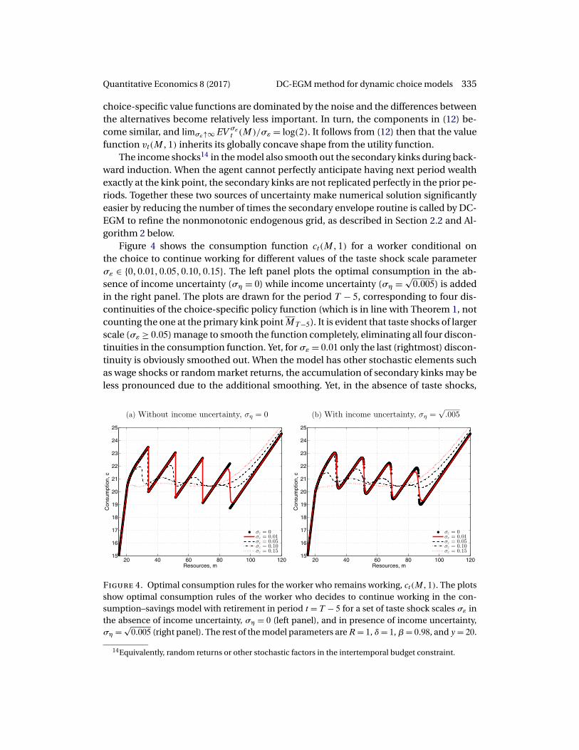
Figure 4 shows the consumption function ct(M�1) for a worker conditional onthe choice to continue working for different values of the taste shock scale parameterσε ∈ {0�0�01�0�05�0�10�0�15}. The left panel plots the optimal consumption in the ab-sence of income uncertainty (ση = 0) while income uncertainty (ση = √
0�005) is addedin the right panel. The plots are drawn for the period T − 5, corresponding to four dis-continuities of the choice-specific policy function (which is in line with Theorem 1, notcounting the one at the primary kink point MT−5). It is evident that taste shocks of largerscale (σε ≥ 0�05) manage to smooth the function completely, eliminating all four discon-tinuities in the consumption function. Yet, for σε = 0�01 only the last (rightmost) discon-tinuity is obviously smoothed out. When the model has other stochastic elements suchas wage shocks or random market returns, the accumulation of secondary kinks may beless pronounced due to the additional smoothing. Yet, in the absence of taste shocks,
Figure 4. Optimal consumption rules for the worker who remains working, ct(M�1). The plotsshow optimal consumption rules of the worker who decides to continue working in the con-sumption–savings model with retirement in period t = T − 5 for a set of taste shock scales σε inthe absence of income uncertainty, ση = 0 (left panel), and in presence of income uncertainty,ση = √
0�005 (right panel). The rest of the model parameters are R= 1, δ= 1, β = 0�98, and y = 20.
14Equivalently, random returns or other stochastic factors in the intertemporal budget constraint.

336 Iskhakov, Jørgensen, Rust, and Schjerning Quantitative Economics 8 (2017)
the primary kinks cannot be avoided even if all secondary kinks are eliminated by a suf-ficiently high degree of uncertainty in the model. It is in this setup, which also appearsto be mostly used in practical applications, where the introduction of the extreme valuedistributed taste shocks is especially beneficial. The taste shocks and other structuralshocks together contribute to the reduction of the number of secondary kinks and tothe alleviation of the issue of their multiplication and accumulation. It is clear from theright panel of Figure 4 that discontinuities in the consumption function can be elimi-nated with a smaller taste shock (σε = 0�01) when additional smoothing through othertypes of uncertainty is present in the model.
Because the expected value function in (14) is a smooth function of M around thepoint where vt(M�1) = vt(M�0), the maximand in (13) is also smooth in this region. Thisleads to an additional benefit of the inclusion of taste shocks, namely that standard nu-merical integration algorithms for the smooth function can be used when calculatingthe integral in (13). When σε = 0, using procedures like Gaussian quadrature typicallyresults in spurious discontinuities as shown in the left panel of Figure 5. This is due tothe integrand not being a smooth function; see Appendix B for a detailed discussion.The right panel of Figure 5 illustrates how moderate smoothing (σε = 0�05) significantlyreduces this approximation error and removes the artificial kinks.
When the taste shocks εt have an interpretation as stochastic noise that is intro-duced to help solve a difficult DC dynamic program by making it more smooth, σε isthe amount of smoothing and has to be chosen and fixed prior to estimation. Theo-rem 3 shows that the level of σε can always be chosen in such a way that the perturbedmodel approximates the underlying deterministic model with an arbitrary degree of pre-cision.
Figure 5. Artificial discontinuities in consumption functions, σ2η = 0�01, t = T − 3. The figure
illustrates how the number of discrete points used to approximate expectations regarding futureincome affects the consumption functions from value function iteration (VFI) and DC-EGM.Panel (a) illustrates how using few (10) discrete equiprobable points to approximate expecta-tions produce severe approximation error when there is no taste shocks. Panel (b) illustrates howmoderate smoothing (σε = 0�05) significantly reduces this approximation error.

Quantitative Economics 8 (2017) DC-EGM method for dynamic choice models 337
Theorem 3 (Extreme Value Homotopy Principle). In every time period the (expected)value function of the consumption and retirement problem with extreme value tasteshocks EV σε
t (Mt) defined in (14) converges uniformly to the value function of the sameproblem without taste shocks Vt(M�1) defined in (2) as the scale of these shocks ap-proaches zero. The uniform bound
∀t: supM≥0
∣∣EV σεt (M�1)− Vt(M�1)
∣∣≤ σε
[T−t∑j=0
βj
]log(2) (16)
holds. Consequently, as σε ↓ 0, both continuous and discrete decision rules of thesmoothed model with taste shocks converge pointwise to those of the deterministic model.
In Appendix D we prove a more general version of Theorem 3 that holds under weakconditions for arbitrary DC models. Theorem 3 formalizes the results presented graph-ically in Figure 4, and justifies our claim that the extreme value smoothing can be re-garded as a homotopy method for solving the nonsmooth limiting problem withouttaste shocks by solving a smooth “nearby” problem with extreme value taste shocks. Theextreme value scale parameter σε plays the role of the “homotopy parameter.”
3.2 Extending DC-EGM for taste shocks and income uncertainty
In the presence of taste shocks and income uncertainty, the DC-EGM algorithm remainslargely the same, and potentially even simpler because the calculation of the primarykinks Mt is replaced by the calculation of choice probabilities using formula (15). Thebiggest difference is that with taste shocks, the DC-EGM operates on the choice-specificvalues, as was mentioned in Section 3.1. We present the pseudo-code of the full algo-rithm in this section.
If we continue to assume that retirement is an absorbing state, the problem of theretiree remains the same, and we focus again on the worker’s problem. With taste andincome shocks it is given by (12), (3), and (13), with the modified “smoothed” Euler equa-tion taking the form15
0 = u′(c)−βR
∫ [u′(ct+1
(R(M − c)+ yη�1
))Pt+1
(1|R(M − c)+ yη
)+ u′(ct+1
(R(M − c)+ yη�0
))Pt+1
(0|R(M − c)+ yη
)]f (dη)
= 1c
−βR
∫ [Pt+1
(1|R(M − c)+ yη
)ct+1
(R(M − c)+ yη�1
) + Pt+1(0|R(M − c)+ yη
)ct+1
(R(M − c)+ yη�0
)]f (dη)�(17)
where Pt(1|M) and Pt(0|M) are the choice probabilities (15), and the last line is writtenfor the case u(c) = log(c).
Given the next period choice-specific consumption functions of the workerct+1(M�0) and ct+1(M�1), we solve (17) via the same backward induction process as
15See Lemma 1 in Appendix A.

338 Iskhakov, Jørgensen, Rust, and Schjerning Quantitative Economics 8 (2017)
described in Section 2.2 for the retirement problem without stochastic shocks. As be-fore, the induction starts at the terminal period T with the easily derived consumptionfunctions cT (M�0) = cT (M�1) = M , choice-specific value functions vT (M�0) = u(M) =vT (M�1)+ δ, and the probability of remaining working PT (1|M)= 1/(1 + exp(δ/σε)).
Then working backward, we choose an exogenous grid over saving �A= (A1� � � � �AJ)
(which remains fixed throughout the backward induction process here for notationalsimplicity) and compute optimal consumption {ct(A1�d)� � � � � ct(AJ�d)} for each pointAj and for each discrete choice d by calculating the inverse marginal utility of the righthand side of the Euler equation (17) and (11) for d = 1 and d = 0, respectively. Us-ing these consumption functions, we construct the endogenous grid over M as �Md
t =(Md
t�1� � � � �Mdt�J), where Md
j is given by Mdj�t = ct(Aj�d)+Aj , j ∈ {1� � � � � J}.
For every d, if the resulting grid points are a monotonically increasing sequence,then no violation of monotonicity of the saving function as per Theorem 2 is indicated,and the DC-EGM method automatically reverts to the standard EGM method of Carroll(2006). However, if �Md
t is not a monotonically increasing sequence, we apply the sameupper envelope procedure as described in Section 2.2 to eliminate the suboptimal ele-ments of �Md
t and add a point where the disjoint segments of the value function intersect.The last step amounts to calculating the choice-specific value functions v(M�d) along-side the consumption functions, which is achieved by plugging the computed ct(A1� d)
into the maximand of the Bellman equation (13) for each point Aj of the exogenous gridon savings.
After the choice-specific consumption and value functions c(M�d) and v(M�d) arecomputed on the monotonic endogenous grids �M∗dt , the period t iteration of the DC-EGM algorithm is complete. Unlike in Section 2.2, in the presence of taste shocks thecalculation of the upper envelope over the choice-specific value functions is not per-formed. Instead, the discrete choice probabilities may be calculated using (15) for anylevel of wealth M using interpolation of the choice-specific values v(M�0) and v(M�1).
We continue this procedure from period T − 1 backward to period t = 1, at whichpoint we have fully approximated the solution to the life-cycle retirement problem byDC-EGM. Note that as before, in the formulation with taste shocks none of the steps ofthe DC-EGM algorithm require iterative root-finding operations.
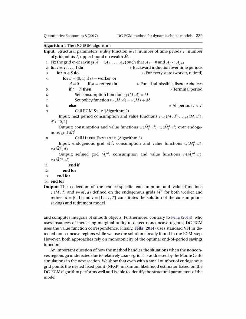
Algorithms 1, 2, and 3 provide the pseudo-code for the complete DC-EGM algorithmfor the problems with discrete shocks. The full DC-EGM algorithm (Algorithm 1) invokesthe EGM step (Algorithm 2) repeatedly to compute the value function correspondencesfor all discrete choices, and then finds and removes all suboptimal points on the re-turned endogenous grids by calling the upper envelope module (Algorithm 3). By Theo-rem 3, it can also approximate the solution for the problems without taste shocks if thescale parameter σε is fixed at a sufficiently small value.
While the DC-EGM is similar to the approach proposed in Fella (2014), we explic-itly allow for extreme value type I taste shocks to preferences and show how they helpwith the computational issues specific to the model of discrete-continuous choices.The approach in Fella (2014) does not readily apply to the class of models with tasteshocks but should be adjusted along the lines described here. In particular, DC-EGMoperates with discrete choice-specific value functions and optimal consumption rules,
Quantitative Economics 8 (2017) DC-EGM method for dynamic choice models 339
Algorithm 1 The DC-EGM algorithm
Input: Structural parameters, utility function u(c), number of time peiods T , numberof grid points J, upper bound on wealth M .
1: Fix the grid over savings �A= {A1� � � � �AJ} such that A1 = 0 and Aj <Aj+1
2: for t = T� � � � �1 do � Backward induction over time periods3: for st ∈ S do � For every state (worker, retired)4: for d = {0�1} if st = worker, or
d = 0 if st = retired do � For all admissible discrete choices5: if t = T then � Terminal period6: Set consumption function cT (M�d)=M
7: Set policy function vT (M�d)= u(M)+ dδ
8: else � All periods t < T
9: Call EGM Step (Algorithm 2)Input: next period consumption and value functions ct+1(M�d′), vt+1(M�d′),
d′ ∈ {0�1}Output: consumption and value functions ct( �Md
t �d), vt( �Mdt �d) over endoge-
nous grid �Mdt
10: Call Upper Envelope (Algorithm 3)Input: endogenous grid �Md
t , consumption and value functions ct( �Mdt �d),
vt( �Mdt �d)
Output: refined grid �M∗dt , consumption and value functions ct( �M∗d
t � d),vt( �M∗d
t � d)
11: end if12: end for13: end for14: end forOutput: The collection of the choice-specific consumption and value functions
ct(M�d) and vt(M�d) defined on the endogenous grids �Mdt for both worker and
retiree, d = {0�1} and t = {1� � � � �T } constitutes the solution of the consumption–savings and retirement model
and computes integrals of smooth objects. Furthermore, contrary to Fella (2014), whouses instances of increasing marginal utility to detect nonconcave regions, DC-EGMuses the value function correspondence. Finally, Fella (2014) uses standard VFI in de-tected non-concave regions while we use the solution already found in the EGM-step.However, both approaches rely on monotonicity of the optimal end-of-period savingsfunction.
An important question of how the method handles the situations when the noncon-vex regions go undetected due to relatively coarse grid �A is addressed by the Monte Carlosimulations in the next section. We show that even with a small number of endogenousgrid points the nested fixed point (NFXP) maximum likelihood estimator based on theDC-EGM algorithm performs well and is able to identify the structural parameters of themodel.

340 Iskhakov, Jørgensen, Rust, and Schjerning Quantitative Economics 8 (2017)
Algorithm 2 The EGM step, adaptation of the standard EGM algorithm (Carroll (2006))
Input: Structural parameters, utility function u(c), current period t < T , state (st),discrete choice d, next period consumption and value functions ct+1(M�d′),vt+1(M�d′), d′ ∈ {0�1}, exogenous grid over savings �A= {A1� � � � �AJ}
1: for j = 1� � � � � J do � Loop over points in �A2: Calculate next period wealth M ′ =AjR+ dyη
3: Calculate next period choice probabilities Pt+1(d′|M ′)
4: Calculate optimal choice-specific consumption ct+1(M′� d′) and u′(ct+1(M
′� d′))5: Calculate choice-specific value function vt+1(M
′� d′) in period t + 16: Repeat Steps 2–5 to compute the right hand side (RHS) of the Euler equation (17)
and the expectation of the next period value function EV (the last component of themaximand in (13)). Gaussian quadrature or other numerical integration algorithmscan be used to calculate the integral over income shocks η. Also, in general case, itmay be necessary to integrate over the transition probabilities P(st ′|st� d) of the stateprocess st, which is trivial in the retirement model.
7: Compute current period optimal consumption c(Aj�d)= (u′)−1(RHS)8: Compute current period choice-specific value function v(Aj�d) = u(c(Aj�d)) +
dδ+ EV9: Compute the endogenous point Md
j�t = c(Aj�d)+Aj
10: end for11: Add an extra point Md
0�t = 0 to �Mdt and set c(0� d) = 0
Output: Endogenous grid �Mdt , consumption and value functions ct( �Md
t �d), vt( �Mdt �d)
over it
3.3 Credit constraints
Before turning to the Monte Carlo results, we briefly discuss how DC-EGM handles thecredit constraints, c ≤ M . During the EGM step, the credit constraints are dealt with inexactly same manner as in Carroll (2006), as described in Section 2.2. Let the smallestpossible end-of-period resources A1 = 0 be the first point in the exogenous grid oversaving �A. Assuming that the corresponding point of the endogenous grid Mt(A1� d) isnonnegative,16 it holds that A(M�d) = 0 for all M ≤ Mt(A1� d) due to the monotonicityof the saving function A(M�d) = M − ct(M�d) (see Theorem 2). Therefore, the optimalconsumption in this region is then given by ct(M�d)= M , and the choice-specific valuefunction is
vt(M�d)= log(M)− dδt +β
∫EV t+1(dyη)f (dη)� M ≤Mt(A1� d)� (18)
Note that the third component of (18) is the expected value of having zero savings. It iscalculated within the EGM step for the point A1 = 0, and should be saved separately asa constant that depends on d but not on M . Once this constant is computed, vt(M�d)
16It is not hard to show that this holds as long as the per-period utility function satisfies the Inada condi-tions.

Quantitative Economics 8 (2017) DC-EGM method for dynamic choice models 341
Algorithm 3 Upper envelope
Input: Endogenous grid �Mdt , choice-specific consumption and value functions
ct( �Mdt �d), vt( �Md
t �d) calculated on �Mdt
1: for j = 1� � � � � J − 1 do2: if Md
j�t >Mdj+1�t then � Detect nonmonotonicity in the endogenous grid
3: Find j′ > j such that Mdj′+1�t >Md
j′�t4: Define partitions �N1 = {1� � � � � j}, �N2 = {j� � � � � j′}, �N3 = {j′� � � � � J}5: Run upper envelope calculation over segments of the “value function corre-
spondence” vt( �N1� d), vt( �N2� d) and vt( �N3� d) computed on the partitions in previ-ous step, as described in Section 2.2 and illustrated in Figure 1, panels (b) and (d).
6: Determine a set of suboptimal grid points Q7: Refine the endogenous grid by removing suboptimal points, so that �M∗d
t =�Mdt \Q
8: Remove the corresponding points ct( �MdQ�t� d), vt( �Md
Q�t� d)
9: [Optional] Add the kink point(s) M where the uppermost segments in Step 5intersect and add the corresponding interpolated values of ct(M�d), vt(M�d)
10: end if11: end forOutput: Refined monotonic grid �M∗d
t , consumption and value functions ct( �M∗dt � d),
vt( �M∗dt � d) calculated on �M∗d
t
essentially has analytical form in the interval [0�Mt(A1� d)], and thus can be directlyevaluated at any point.
When the per-period utility function is additively separable in consumption and dis-crete choice as in the retirement model we consider, (18) holds for all d in the inter-val 0 ≤ M ≤ mind Mt(A1� d). In other words, the choice-specific value functions for lowwealth have the same shape, which is shifted vertically with dt-specific coefficients. Thisimplies that the logistic choice probabilities Pt(d|M) are constant in this interval andhave to be calculated only once.
4. Monte Carlo results
In this section we investigate the properties of the approximate maximum likelihoodestimator (MLE) that we obtain using the DC-EGM to approximate the model solutionin the inner loop of the nested fixed point algorithm. We specifically focus on the role ofincome uncertainty and taste shocks for the approximation bias induced by a numericalsolution with a finite number of grid points; in particular, how approximation bias de-pends on the number of grid points in smooth as well as nonsmooth problems. After adescription of the data generating process (DGP), we present the results from a series ofMonte Carlo experiments, and show that models used in typical empirical applicationsare sufficiently smooth to almost eliminate approximation bias using relatively few gridpoints.

342 Iskhakov, Jørgensen, Rust, and Schjerning Quantitative Economics 8 (2017)
4.1 Data generation process
For the Monte Carlo we consider a slightly more general formulation of the con-sumption–savings and retirement problem defined in (1) with constant relative riskaversion (CRRA) utility
max{ct �dt }T1
T∑t=1
βt
(c
1−ρt − 11 − ρ
− δtdt + σεε(dt)
)� (19)
where ρ is the CRRA coefficient.So as to simulate synthetic data from the DGP consistent with the model and the
vector of true parameter values, we solve the model very accurately with 2000 grid pointsusing the DC-EGM. We refer to this solution as the true solution even though this is ofcourse only an accurate finite approximation of the value function.17
We consider several specifications of the model in the Monte Carlo experiments be-low to study various aspects of the performance of the estimator. Our monte carlo exper-iments focus on estimation of the parameter δ for the disutility of work18, which we as-sume is time-invariant with a true values shown in Table 1. We perform 200 Monte Carloreplications for each of the combinations of the other parameters, which are treated asknown and fixed at their true values listed in Table 1. The exception is Section 4.4 wherethe true value of σε used to generate the data is zero, but where we impose that σε iseither 0�01 or 0�05. This enables us to also study the effect of model misspecification onthe Monte Carlo performance of the NFXP estimator using the DC-EGM algorithm.
For each specification of the model, 50,000 individuals are simulated for T = 44 pe-riods. Each individual i is initiated as a full-time worker sdi�1 = 1, where we have used
sdi�t ∈ {0�1} to denote the labor market state, that is, whether an individual is retired
(sdi�t = 0) or working (sdi�t = 1). Each worker’s initial wealth Mdi�1 is drawn from a uniform
distribution on the interval [0�100]. At the beginning of each time period t, a randomlog-normal labor market income shock ηt with variance parameter ση is drawn if theindividual i is working and the individual’s resources Md
t are calculated. Given the level
Table 1. Baseline true parameter values.
Description Value Description Value
Time horizon T = 44 Disutility of work δ ∈ {0�1�0�5}Gross interest rate R = 1�03 Discount factor β= 0�97Full time employment income y = 1�0 CRRA coefficient ρ= 2�0Income variance ση = 0 Taste shocks scale σε ∈ {0�0�01�0�05}
17As a spot check, we have also compared this solution with the traditional value function iteration ap-proach, where we used a grid search over 1000 discrete points on the interval [0�Mt ] to locate the optimalconsumption for each value of wealth. We find that results are essentially identical.
18Other parameters insluding the scale of taste shocks σε could have been estimated as well, but for clearexposition we focus on a single parameter.

Quantitative Economics 8 (2017) DC-EGM method for dynamic choice models 343
of resources, discrete choice-specific value functions and choice probabilities are com-puted, and a random draw determines which discrete labor market option ddit is cho-sen. The labor force participation decision at t becomes the labor market state at t + 1,sdi�t+1 = ddit . The optimal level of consumption, cit , is then computed conditional on ddit ,and the end-of-period wealth is calculated and stored to be used for calculation of re-sources available in the beginning of period t + 1, Md
i�t+1. We then add normal addi-tive measurement error with standard deviation σξ = 1 to get the simulated consump-tion data, cdit . This produces simulated panel data (Md
it� sdit � d
dit � c
dit) for each individual
i ∈ {1� � � � �50,000} in all time periods t ∈ {1� � � � �44}.
4.2 Maximum likelihood estimation
We implement a discrete-continuous version of the nested fixed point (NFXP) maximumlikelihood estimator devised in Rust (1987, 1988), where we augment the original dis-crete choice estimator with a measurement error approach when assessing the likeli-hood of the observed continuous choices.
Assume that a panel data set is available, {(Mdit� s
dit � d
dit � c
dit)}i={1�����N}�t={1�����T }, con-
taining observations on wealth, labor market state, and discrete and continuous choicesof individuals i = 1� � � � �N in time periods t = 1� � � � �T . Let ct(Mt� st� dt |θ) denote theconsumption policy function computed by the DC-EGM for a given vector of model pa-rameters θ = (δ�β�ρ�ση�σε). We assume that consumption is observed with additiveGaussian measurement error,
cdit = ct(Md
it� sdit � d
dit |θ
)+ ξit� ξit ∼N(0�σξ)� i.i.d. ∀i� t� (20)
Let ξdit(θ) = cdit − ct(Mdit� s
dit � d
dit |θ) denote the difference between the predicted and the
observed consumption. We assume that the measurement error, ξit , is independent ofthe taste shocks, εt(dt), and, thus, the joint likelihood of observation i in period t is givenby
it(θ�σξ) = P(ddit |Md
it� sdit � θ
)φ(ξdit(θ)/σξ
)σξ
� (21)
where φ(·) is the density function of the standard normal distribution. We have ignoredthe controlled transition probability for the retirement status sdit , since Ptr(s
dit |sdi�t−1�
ddi�t−1) is always 1 in the data when retirement is absorbing and the labor market state isperfectly controlled by the decision.
The choice probabilities for the workers (sdit = 1) are standard logits,
P(ddit |Md
it� sdit � θ
)= exp(vt(Md
it� sdit � d
dit |θ
)/σε
)1∑
j=0
exp(vt(Md
it� sdit � j|θ
)/σε
) � (22)
and are computed from the discrete choice-specific value functions vt(Mdit� s
dit � d
dit |θ)
found by the DC-EGM given a particular value of the parameter vector θ, evaluated at

344 Iskhakov, Jørgensen, Rust, and Schjerning Quantitative Economics 8 (2017)
the data. Because retirement is absorbing and thus retirees do not have any discretechoice to make, the first component of individual likelihood contribution (21) drops outwhen sdit = 0.
The joint log-likelihood function is given by L(θ�σξ) = log∏N
i
∏Tt it(θ�σξ), where
rearranging the first order condition with respect to σ2ξ yields the standard MLE for the
measurement error variance, σ2ξ(θ) = 1
NT
∑Tit=1 ξ
dit(θ)
2. The concentrated log-likelihoodfunction is, therefore, proportional to
L(θ)∝N∑i=1
T∑t=1
{sditσε
(vt(Md
itsdit � d
dit |θ
)− EV t(Md
it� sdit |θ
))− 12
log
(N∑i=1
T∑t=1
ξdit(θ)2
)}� (23)
where EV t (Mdit� s
dit |θ) is the the log sum given in (14) evaluated at parameter value θ.19
The parameter vector θ that maximizes (23) is the MLE of the model parameters.
4.3 Taste shocks as unobserved state variables
We are now ready to investigate the effects of smoothing on the accuracy of the MLEbased on the DC-EGM algorithm. We conduct two Monte Carlo experiments where wevary the degree of smoothing induced by extreme value taste shocks and income un-certainty, respectively. Throughout we focus on estimating the parameter that indexesdisutility of work, δ, while keeping all others fixed at their true values. Appendix C con-tains the average estimation time for DC-EGM.
Taste shocks and approximation error Figure 6 displays the root mean square error(RMSE) of the parameter estimates for the disutility of work, δ. Results are shown forvarying degrees of smoothing, σε ∈ {0�01�0�05}, and different values of the disutility of
Figure 6. Monte Carlo results: disutility of work. The plots illustrate the root mean square error(RMSE) of δ. Results are shown for varying degrees of smoothing, σε ∈ {0�01�0�05}, and differentvalues of the disutility of work, δ ∈ {0�1�0�5}. The rest of the parameters are at their baseline levels;see Table 1.
19Following (23), the log sum only has to be evaluated for workers, sdit = 1.

Quantitative Economics 8 (2017) DC-EGM method for dynamic choice models 345
work parameter, δ ∈ {0�1�0�5}. With RMSE around 1�0e−3, the proposed estimator is al-ready accurate with 50 grid points and rapidly improves as the number of grid pointsincreases from 50 through 1000. Note that standard errors will of course increase withσε due to the increased amount of unexplained variation in the error term, and RMSEreflects this too. Bearing this is mind, it is evident that the approximation bias decreasesas the degree of smoothing increases, that is, larger values of σε. For higher levels ofsmoothing, problems with multiplicity of the Euler equation solutions disappear andfew grid points are needed to approximate the (smooth) consumption function. This isparticularly true when the disutility from work is large (δ = 0�5) because the noncon-cave regions are larger in this case. We also calculated the Monte Carlo standard devia-tion (MCSD),20 which is on the order of 1�0e−4 irrespective of the number of grid pointsused.
Income uncertainty Additional uncertainty about, for example, future labor market in-come tends to smooth out secondary kinks stemming from multiple solutions to the Eu-ler equations. To illustrate how that additional smoothing affects the proposed estima-tor, Figure 7 display RMSE when introducing income uncertainty. We report results fromtwo different values of the income variance,21 σ2
η ∈ {0�001�0�05}. The first level, 0�001,does not completely smooth out secondary kinks while the significantly more uncertainincome process with σ2
η = 0�05 does (see the right panel of Figure 4).Income uncertainty together with taste shocks smooth the problem to such a degree
that the RMSE drops by an order of magnitude when increasing the income variancefrom 0�001 to 0�05. Hence, using only a few grid points when estimating such a modelwill result in only minor approximation errors.
Figure 7. Monte Carlo results: income uncertainty. The plots illustrate the root mean squareerror (RMSE). Results are shown for varying degrees of smoothing, σε ∈ {0�01�0�05}, and differentvalues of the income variance, σ2
η ∈ {0�001�0�05}. The rest of the parameters are at their baselinelevels; see Table 1.
20MCSD is defined as standard deviation of the difference between the estimates and true values accrossMonte Carlo runs, results not shown.
21The values of the income variance we use correspond well to the empirical findings, for example, inGourinchas and Parker (2002), Meghir and Pistaferri (2004), Imai and Keane (2004).

346 Iskhakov, Jørgensen, Rust, and Schjerning Quantitative Economics 8 (2017)
As mentioned, standard errors will of course increase with σε due to the increasedamount of unexplained variation. The MCSD is quite small and unaffected by the degreeof income uncertainty as well as the number of grid points, but increases from 0�00023to 0�00045 as σε increases from 0�01 to 0�05. This is the main explanation for why RMSEis only smaller for a small number of grid points. Sorting out this effect, it is clear thatincreasing σε decreases the amount of pure approximation bias, especially when thenumber of grid points is small. Note that MCSD is very small, in part due to a relativelylarge sample size, but also because the variance of the i.i.d. extreme value error term isextremely small. In most empirical applications, σε would be larger, leading to an evensmoother problem than the one we consider here. Hence, with relatively few grid pointswe can expect to obtain an even smaller approximation bias induced by the finite gridapproximation in the DC-EGM.
4.4 Taste shocks as logit smoother
Until now we have assumed that the correct model has unobserved state variables and,thus, σε > 0 has to be estimated. To investigate how the proposed estimator performsif the data stem from a model in which there are no unobserved states, we estimateversions of the model where we impose σε > 0 and, thus, estimate a misspecified model.This is interesting because if researchers have reasons to believe that the underlyingmodel has no shocks, the inclusion of these shocks acts as a smooth approximation tothe true deterministic model. As argued above, solving the smoothed model is muchfaster since it requires fewer grid points and, thus, is much faster to estimate.
Figure 8 illustrates the RMSE of δ when using 50, 100, and 500 grid points for var-ious levels of smoothing σε ∈ [0�001�0�05], while the correct level is σε = 0. Intuitively,as the model becomes “more” misspecified (increasing the imposed σε), the RMSE andthe MCSD increase. Interestingly, for a given number of discrete grid points, the RMSE is
Figure 8. Monte Carlo results: true model without taste shocks (misspecified). The plots illus-trate the root mean square error (RMSE) from estimation of a misspecified model. The modelfrom which data are simulated is deterministic, σε = 0, while the model used to estimate thedisutility of work imposes σε > 0. Results are shown for varying degrees of imposed smoothing,σε ∈ [0�001�0�05] on the horizontal axes, different levels of income shocks, ση ∈ {0�0�05}, and dif-ferent number of grid points. The rest of the parameters are at their baseline levels; see Table 1.
Quantitative Economics 8 (2017) DC-EGM method for dynamic choice models 347
minimized by a σε > 0. While large degree of smoothing induces significant approxima-tion bias, the bias is initially falling in σε until some point at which the RMSE increasesagain. The minimum of the RMSE is attained for lower levels of smoothing if additionalstochasticity (i.e., income shocks) is present in the model. This is expected because theincome uncertainty smooths the problem and less logit smoothing is needed to ob-tain the optimal smooth approximation. It is worth noting, however, that the optimalamount of logit smoothing may not be sufficient to completely eliminate the noncon-vexities in the model. It is therefore essential for the solution method to be able to ro-bustly solve optimization problems with multiple local solutions, the task that DC-EGMperforms particularly well.
These results show the potential for great speed gains by smoothing. Using only 50grid points and imposing σε = 0�01 produces a RMSE of around the same level as using500 grid points and imposing σε ≈ 0 close to the true model. We can reduce the numberof grid points by an order of magnitude without increasing the root mean square errorsignificantly simply by choosing the degree of smoothing appropriately. Note, however,that there is naturally a trade-off between lowering the computational cost by increasingsmoothing and decreasing the number of grid points and the accuracy of the resultingsolution compared to the true solution of the nonsmooth model.
5. Discussion and conclusions
In this paper we have shown how complications from numerous discontinuities in theconsumption function to a life-cycle model with discrete and continuous choices canbe avoided by smoothing the problem and using the DC-EGM algorithm. The proposedalgorithm retains all the nice features of the original EGM method, namely that it typ-ically does not require any iterative root-finding operations, and is equally efficient indealing with borrowing constraints. Moreover, we show that the smoothed model canbe successfully estimated by the NFXP estimator based on the DC-EGM algorithm evenwith a small number of grid points and even when the true DGP is nonsmooth.
For expositional clarity, we focused on a simple illustrative example when explainingthe details of the DC-EGM algorithm. This also allows us to derive an analytical solutionthat we can compare to the numerical one. The analytical solution provides economicintuition for why first and second order kinks appear, and permits direct evaluationof the precision of the DC-EGM algorithm. Admittedly, the illustrative model of con-sumption and retirement is very stylized, and the reader may wonder if DC-EGM can beused to solve and estimate larger, more complex, and realistic models with more statevariables, multiple discrete alternatives, heterogeneous agents, institutional constraints,and so forth. The answer is positive. As shown in Appendix A, the DC-EGM method canbe applied to a much more general class of problems as long as the postdecision statevariable is a sufficient statistic for the continuous choice in the current period, and themarginal utility function and intratemporal budget constraint are invertible. When themarginal utility function is analytically invertible, DC-EGM also avoids the bulk of costlyroot-finding operations.22
22The DC-EGM algorithm can also be generalized for other specifications including the models withlarge state space and multidimensional discrete choice. White (2015), Iskhakov (2015), Druedahl and Jør-

348 Iskhakov, Jørgensen, Rust, and Schjerning Quantitative Economics 8 (2017)
The DC-EGM method has been implemented in several recent empirical applica-tions, where it has proven to be a powerful tool for solving and estimating more com-plex DC models in various fields: labor supply, human capital accumulation and saving(Iskhakov and Keane (2016)); joint retirement decisions of couples (Jørgensen (2014));consumption, housing purchases, and housing debt (Yao, Fagereng, and Natvik (2015));saving decisions and fertility (Ejrnæs and Jørgensen (2016)); precautionary borrowingand credit card debt (Druedahl and Jørgensen (2015)).
We have demonstrated in the Monte Carlo experiments that the NFXP maximumlikelihood estimator based on the DC-EGM solution algorithm performs very well whendecisions are made under uncertainty, for example, in the presence of extreme valuedtaste shocks and the existence of income uncertainty. Even when the true model is de-terministic, taste shocks can be used as a powerful smoothing device to simplify thesolution without much approximation bias due to oversmoothing.
The addition of extreme value taste shocks is not only a convenient smoothing de-vice that simplifies the solution of DC models, it is also an empirically relevant extensionrequired to avoid statistical degeneracy of the model. In empirical applications the vari-ance of these shocks is typically much larger compared to what we have considered here.This makes models smooth enough to almost eliminate approximation bias in parame-ter estimates even with relatively few grid points. We therefore conclude that DC-EGMis practical and appears to be a fast and accurate method for use in actual empiricalapplications.
Appendix A: Theoretical foundations of DC-EGM
For the purpose of this Appendix we consider the following more general formulation ofthe consumption–savings and retirement problem. Let Mt denote consumable wealththat is a continuous state variable with particular motion rule described below, and letst denote a vector of additional discrete or discretized state variables. Let ct be the scalarcontinuous decision (consumption) and let dt be a scalar discrete decision variable withfinite set of values that could encode multiple discrete decisions if needed. Consider thedynamic discrete-continuous choice problem given by the Bellman equation,
Vt(Mt� st) = max0≤ct≤Mt�dt∈Dt
[u(ct� dt� st)+ σεεt(dt)+βtEt
{Vt+1(Mt+1� st+1)|At�dt
}]� (24)
where t = 1� � � � �T − 1, and the last component of the maximand is absent for t = T . Thechoices in the model are restricted by the credit constraint ct ≤ Mt and feasibility setsDt . The per-period utility includes scaled taste shocks σεεt(dt), where εt is a vector ofi.i.d. extreme value (type I) distributed random variables. The dimension of εt is equalto the number of alternatives that the discrete choice variable may take, εt(dt) denotesthe component that corresponds to a particular discrete decision. In the general casethe discount factor βt is time-specific to allow for the probability of survival. The ex-pectation is taken over the taste shocks εt+1 and the transition probabilities of the state
gensen (2017) present theoretical foundations for extending endogenous grid methods to multidimen-sional models.

Quantitative Economics 8 (2017) DC-EGM method for dynamic choice models 349
process st as well as any serially uncorrelated (or idiosyncratic) shocks that may affectMt+1 and st+1. The expectation is taken conditional on the choices in period t using thesufficient statistic At =Mt − ct in place of the continuous (consumption) choice.
Using the well known representation of the expectation of the maximum of extremevalue distributed random variables, the Bellman equation (24) can be written in termsof the deterministic choice-specific value functions as
vt(Mt� st |dt) = max0≤ct≤Mt
[u(ct� dt� st)+βtEt
{Vt+1(Mt+1� st+1)|At�dt
}](25)
= max0≤ct≤Mt
[u(ct� dt� st)
+βtEt{φ(vt+1(Mt+1� st+1|dt+1)�Dt+1�σε
)|At�dt}]�
(26)
where φ(xj� J�σ)= σ log[∑j∈J exp xjσ ] is the log-sum function. The expectation in (26) is
now only taken with respect to (w.r.t.) state transitions and idiosyncratic shocks, unlikein (24) and (25).
The crucial assumption for the DC-EGM is that postdecision state At constitutes thesufficient statistic for the continuous choice in period t, that is, that transition proba-bilities/densities of the state process (Mt� st) depend on At rather than Mt or ct directly.It is also required that At as a function of Mt is (analytically) invertible. For our case,assume for concreteness that At = Mt − ct , and that Mt+1 = RAt + y(dt), where R is agross return, and y(dt) is discrete choice-specific income. We also assume that the utilityfunction u(ct� dt� st) satisfies the following condition.
Assumption A (Concave Utility). The instantaneous utility u(ct� dt� st) is concave23 in ctand has a monotonic derivative w.r.t. ct that is (analytically) invertible.
Lemma 1 (Smoothed Euler Equation). The Euler equation for the problem (24) takes theform
u′(ct� dt� st)
= βtREt
[ ∑dt+1∈Dt+1
u′(ct+1(Mt+1� st+1|dt+1)�dt+1� st+1)Pt+1(dt+1|Mt+1� st+1)
]�
(27)
where u′(ct� dt� st) is the partial derivative of the utility function w.r.t. ct , ct+1(Mt+1�
st+1|dt+1) is the choice-specific consumption function in period t+1, and Pt+1(dt+1|Mt+1�
st+1) is the conditional discrete choice probability in period t + 1, given by
Pt(dt |Mt� st) = exp(vt(Mt� st |dt)/σε
)/ ∑d∈Dt
exp(vt(Mt� st |d)/σε
)� (28)
23More precisely, a weaker condition is sufficient, namely for every x and arbitrary �1 > 0 and �2 > 0 itmust hold that u(ct +�1� dt� st )− u(ct � dt� st ) ≥ u(ct +�1 +�2� dt� st )− u(ct +�2� dt� st ); see Theorem 2.
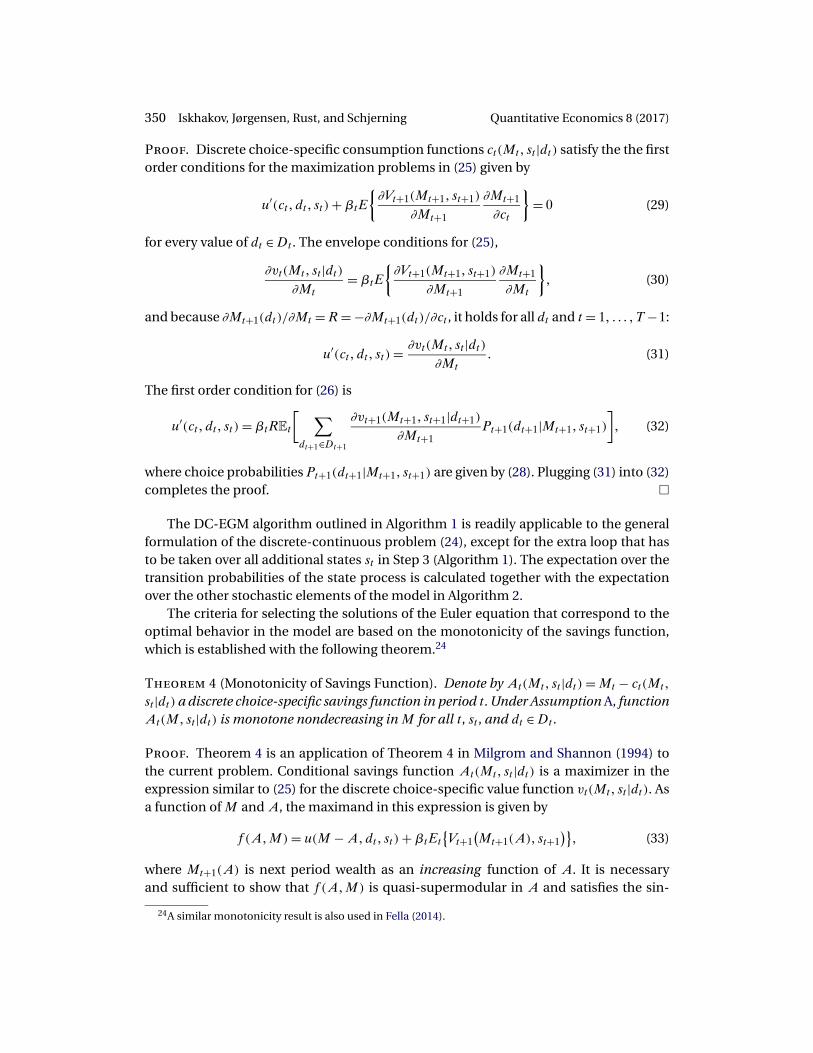
350 Iskhakov, Jørgensen, Rust, and Schjerning Quantitative Economics 8 (2017)
Proof. Discrete choice-specific consumption functions ct(Mt� st |dt) satisfy the the firstorder conditions for the maximization problems in (25) given by
u′(ct� dt� st)+βtE
{∂Vt+1(Mt+1� st+1)
∂Mt+1
∂Mt+1
∂ct
}= 0 (29)
for every value of dt ∈Dt . The envelope conditions for (25),
∂vt(Mt� st |dt)∂Mt
= βtE
{∂Vt+1(Mt+1� st+1)
∂Mt+1
∂Mt+1
∂Mt
}� (30)
and because ∂Mt+1(dt)/∂Mt =R= −∂Mt+1(dt)/∂ct , it holds for all dt and t = 1� � � � �T −1:
u′(ct� dt� st) = ∂vt(Mt� st |dt)∂Mt
� (31)
The first order condition for (26) is
u′(ct� dt� st) = βtREt
[ ∑dt+1∈Dt+1
∂vt+1(Mt+1� st+1|dt+1)
∂Mt+1Pt+1(dt+1|Mt+1� st+1)
]� (32)
where choice probabilities Pt+1(dt+1|Mt+1� st+1) are given by (28). Plugging (31) into (32)completes the proof. �
The DC-EGM algorithm outlined in Algorithm 1 is readily applicable to the generalformulation of the discrete-continuous problem (24), except for the extra loop that hasto be taken over all additional states st in Step 3 (Algorithm 1). The expectation over thetransition probabilities of the state process is calculated together with the expectationover the other stochastic elements of the model in Algorithm 2.
The criteria for selecting the solutions of the Euler equation that correspond to theoptimal behavior in the model are based on the monotonicity of the savings function,which is established with the following theorem.24
Theorem 4 (Monotonicity of Savings Function). Denote by At(Mt� st |dt) = Mt − ct(Mt�
st |dt) a discrete choice-specific savings function in period t. Under Assumption A, functionAt(M� st |dt) is monotone nondecreasing in M for all t, st , and dt ∈Dt .
Proof. Theorem 4 is an application of Theorem 4 in Milgrom and Shannon (1994) tothe current problem. Conditional savings function At(Mt� st |dt) is a maximizer in theexpression similar to (25) for the discrete choice-specific value function vt(Mt� st |dt). Asa function of M and A, the maximand in this expression is given by
f (A�M) = u(M −A�dt� st)+βtEt{Vt+1
(Mt+1(A)� st+1
)}� (33)
where Mt+1(A) is next period wealth as an increasing function of A. It is necessaryand sufficient to show that f (A�M) is quasi-supermodular in A and satisfies the sin-
24A similar monotonicity result is also used in Fella (2014).

Quantitative Economics 8 (2017) DC-EGM method for dynamic choice models 351
gle crossing property in (A�M). The former is trivial because A is a scalar. For the latter,consider A′ >A′′, M ′ >M ′′ and assume f (A′�M ′′) > f(A′′�M ′′). Then
f(A′�M ′)− f
(A′′�M ′)
= u(M ′ −A′� dt� st
)− u(M ′ −A′′� dt� st
)+βt
[EV t+1
(Mt+1
(A′)� st+1
)− EV t+1(Mt+1
(A′′)� st+1
)]≥ u
(M ′′ −A′� dt� st
)− u(M ′′ −A′′� dt� st
)+βt
(EV t+1
(Mt+1
(A′)� st+1
)− EV t+1(Mt+1
(A′′)� st+1
))= f
(A′�M ′′)− f
(A′′�M ′′)> 0�
(34)
For the first inequality we use
u(M ′ −A′� dt� st
)− u(M ′ −A′′� dt� st
)≥ u(M ′′ −A′� dt� st
)− u(M ′′ −A′′� dt� st
)�
u(M ′ −A′� dt� st
)− u(M ′′ −A′� dt� st
)≥ u(M ′ −A′′� dt� st
)− u(M ′′ −A′′� dt� st
)�
u(z�dt� st)− u(z −�M�dt� st) ≥ u(z +�A�dt� st)− u(z +�A −�M�dt� st)�
(35)
where z = M ′ − A′, �A = A′ − A′′ > 0, and �M = M ′ − M ′′ > 0, and which is due to As-sumption A, that is, concavity of the utility function. It follows then that f (A′�M ′) >f(A′′�M ′). Similarly, assumption f (A′�M ′′) ≥ f (A′′�M ′′) leads to f (A′�M ′) ≥ f (A′′�M ′)and, thus, f (A�M) satisfies the single crossing property, and the monotonicity theoremin Milgrom and Shannon (1994) applies. �
Appendix B: Spurious discontinuities from numerical integration
To illustrate how naive numerical quadrature integration can produce spurious discon-tinuities in the policy function, we here focus on the illustrative model without smooth-ing. Particularly, for working households, the smoothed Euler equation in (17) collapsesto
u′(ct(Mt |dt))= β
∫ ∞
0Ru′(ct+1(Mt+1|dt+1 = 1)
) · 1{Mt+1 ≤ Mt+1}f (dη)
+β
∫ ∞
0Ru′(ct+1(Mt+1|dt+1 = 0)
) · 1{Mt+1 >Mt+1}f (dη)�(36)
where we recall that Mt+1 = R(Mt − ct(Mt |dt)) + yη. With the change of variables, q =f (η), we can write the Euler equation (36) as
u′(ct(Mt |dt))= β
∫ qt
0f−1(q)u′(ct+1
(R(Mt − ct(Mt |dt)
)+ yf−1(q)�dt+1 = 1))dq
+β
∫ 1
qt
f−1(q)u′(ct+1(R(Mt − ct(Mt |dt)
)+ yf−1(q)�dt+1 = 0))dq�
(37)

352 Iskhakov, Jørgensen, Rust, and Schjerning Quantitative Economics 8 (2017)
where the threshold qt is given by
qt = f
(Mt+1
Mt+1
)� (38)
As long as the income shock distribution is not degenerate, the resulting Euler equation(37) is continuous and smooth in ct(Mt�W) through Mt+1 in spite of the discontinuityin the consumption function ct+1(Mt+1�W) at Mt+1 = Mt+1. In turn, this suggests thatnumerical integration should be done twice—once for each case—to ensure that theintegral is well behaved.
In contrast, the naive Euler equation in (36) is discontinuous in ct(Mt�W). When us-ing numerical quadrature to evaluate the integral, for a given level of resources, someof the nodes will result in Mt+1 ≤ Mt+1 while others will result in the opposite case. Forconcreteness, say that 10 nodes are used and the five lowest nodes result in Mt+1 ≤Mt+1.Say also that for a slightly larger value of current resources perhaps only four nodes sat-isfy Mt+1 ≤ Mt+1 while now six invoke the alternative. When comparing the solutionfound in the two (close) values of current period resources, there will be a discontinuouschange in the optimal consumption. In the current model, this would result in spuriousdownward kinks in the consumption function around a secondary kink.
Appendix C: DC-EGM run times
Figure 9 illustrates the average estimation time spent to estimate δ. Results are shownfor varying degrees of income uncertainty, ση ∈ {0�001�0�05}, and different values of thedisutility of work parameter, δ ∈ {0�1�0�5}.
Appendix D: Proof of extreme value homotopy principle
This appendix proves Theorem 3, which states that the value function and optimal de-cision rules in the presence of type I extreme value distributed taste shocks converge (inan appropriate sense to be defined below) to the value functions and decision rules of a
Figure 9. Timing: income uncertainty. The plots illustrate the time spent to estimate the model.Results are shown for varying degree of smoothing, σε ∈ {0�01�0�05}, and different values of theincome variance, σ2
η ∈ {0�001�0�05}. The rest of parameters are at their baseline levels; see Table 1.

Quantitative Economics 8 (2017) DC-EGM method for dynamic choice models 353
limiting problem without taste shocks. We prove Theorem 3 for a more general class ofproblems than just the retirement consumption model, and therefore restate it below.
Let ε be a random variable having a standardized type I extreme value distributionwith the cumulative distribution function (CDF) given by
F(ε) = exp{−exp{−ε}}� (39)
We have E{ε} = γ, where γ = 0�577 � � � is Euler’s constant and var(ε) = π2/6. Then if σis a positive scaling constant, σε will also be a type I extreme value distribution withexpected value σγ and variance σ2π2/6. In the notation of the illustrative model in thepaper, σ corresponds to the scaling parameter of the “perturbed” model σε.
The homotopy convergence result we prove below holds for a considerably moregeneral class of dynamic programming (DP) problems than the simple retirement ex-ample we analyzed in Section 2.1 or even the class defined in Appendix A, where we as-sumed the continuous choice is a unidimensional variable and we imposed additionalassumptions to ensure monotonicity of the savings function. In this appendix we con-sider a more general class of problems, though we do not strive for maximum possiblegenerality so as to make our proof as straightforward as possible.
Consider a finite horizon DP problem without type I extreme value taste shocksthat we also refer to as the “unperturbed” DP problem. In the last period, T , the agentchooses a vector of k continuous choice variables c ∈ CT (d� s), where CT (d� s) is a com-pact subset of a Rk, d is one of the discrete choices, and s is a potentially multidimen-sional vector of state variables in some Borel subset S of a finite dimensional Euclideanspace. We assume that the discrete choice d is an element of a finite choice set DT(s).Let uT (d� c� s) be a utility function that is continuous in c for each s and each d ∈ DT(s)
and a Borel measurable function of s for each c and d. Then the value function in periodT is given by
VT (s) = maxd∈DT (s)
maxc∈CT (d�s)
uT (d� c� s)� (40)
Now consider time T − 1 and let pT (s′|s� c�d) be a Markov transition probability provid-
ing the conditional probability distribution over the state s′ at time T given that the statevector at time T − 1 is s, the discrete choice is d, and the continuous choice is c. Definethe conditional expectation of VT , EV T−1(d� c� s), by
EV T−1(d� c� s) =∫
VT(s′)pT
(∂s′|d� c� s)� (41)
where we use ∂s′ to indicate the stochastic next period state variables over which thisexpectation is taken. In Assumption C below, we assume that this conditional expec-tation exists and is continuous in c for each s ∈ S and d ∈ DT−1(s). Then by back-ward induction we can define the value function VT−1(s) and, continuing for eacht ∈ {T − 1�T − 2� � � � �0}, we can define the sequence of functions {Vt} recursively usingBellman’s equation,
Vt(s) = maxd∈Dt(s)
maxc∈Ct(d�s)
[ut(d� c� s)+β
∫Vt+1
(s′)pt+1
(∂s′|d� c� s)]� (42)
where β≥ 0 is the agent’s discount factor.
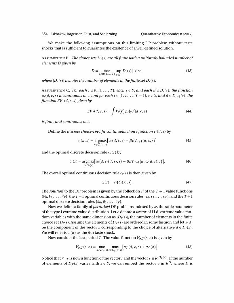
354 Iskhakov, Jørgensen, Rust, and Schjerning Quantitative Economics 8 (2017)
We make the following assumptions on this limiting DP problem without tasteshocks that is sufficient to guarantee the existence of a well defined solution.
Assumption B. The choice sets Dt(s) are all finite with a uniformly bounded number ofelements D given by
D= maxt∈{0�1�����T }
sups∈S
∣∣Dt(s)∣∣<∞� (43)
where |Dt(s)| denotes the number of elements in the finite set Dt(s).
Assumption C. For each t ∈ {0�1� � � � �T }, each s ∈ S, and each d ∈ Dt(s), the functionut(d� c� s) is continuous in c, and for each t ∈ {1�2� � � � �T − 1}, s ∈ S, and d ∈ Dt−1(s), thefunction EV t (d� c� s) given by
EV t (d� c� s) =∫
Vt(s′)pt(∂s′|d� c� s) (44)
is finite and continuous in c.
Define the discrete choice-specific continuous choice function ct(d� s) by
ct(d� s)= argmaxc∈Ct(d�s)
[ut(d� c� s)+βEV t+1(d� c� s)
](45)
and the optimal discrete decision rule δt(s) by
δt(s) = argmaxd∈Dt(s)
[ut(d� ct(d� s)� s
)+βEV t+1(d� ct(d� s)� s
)]� (46)
The overall optimal continuous decision rule ct(s) is then given by
ct(s) = ct(δt(s)� s
)� (47)
The solution to the DP problem is given by the collection Γ of the T + 1 value functions{V0� V1� � � � � VT }, the T +1 optimal continuous decision rules {c0� c1� � � � � cT }, and the T +1optimal discrete decision rules {δ0� δ1� � � � � δT }.
Now we define a family of perturbed DP problems indexed by σ , the scale parameterof the type I extreme value distribution. Let ε denote a vector of i.i.d. extreme value ran-dom variables with the same dimension as |Dt(s)|, the number of elements in the finitechoice set Dt(s). Assume the elements of DT(s) are ordered in some fashion and let ε(d)be the component of the vector ε corresponding to the choice of alternative d ∈ Dt(s).We will refer to ε(d) as the dth taste shock.
Now consider the last period T . The value function Vσ�T (s� ε) is given by
Vσ�T (s� ε) = maxd∈DT (s)
maxc∈CT (d�s)
[uT (d� c� s)+ σε(d)
]� (48)
Notice that Vσ�T is now a function of the vector s and the vector ε ∈ R|DT (s)|. If the numberof elements of DT(s) varies with s ∈ S, we can embed the vector ε in RD, where D is

Quantitative Economics 8 (2017) DC-EGM method for dynamic choice models 355
the upper bound on the number of discrete choices by Assumption B. We can use theconvention that if |DT(s)| < D for some s ∈ S, the function Vσ�T (s� ε) depends only onthe components of ε corresponding to the feasible choices d ∈ DT(s) and not on anycomponents d that are not elements of DT(s).
The CDF F(ε) of the vector random variable ε is given by the product of the univari-ate type I extreme value CDFs, that is,
F(ε(1)� � � � � ε(D)) =D∏
d=1
exp{−exp
{−ε(d)}}� (49)
To compute the expected value of VT (s�ε), we apply multivariate integration to get
EV σ�T (d� c� s) =∫s′
∫ε′Vt(s′� ε′)F(∂ε′)pT
(∂s′|d� c� s)
=∫s′σ log
( ∑d∈DT (s′)
exp{uT
(d� cT (s�d)�d
)/σ
})pT
(∂s′|d� c� s)� (50)
where cT (s�d) = argmaxc∈CT (d�s)uT (d� c� s) is the choice-specific continuous choice
function. The closed-form expression for the expectation over ε′—the type I extremevalue random variables—is a consequence of a property of extreme value random vari-ables known as max stability, that is, the maximum of a finite collection of type I extremevalue random variables has a (shifted) type I extreme value distribution. We refer to thelog-sum formula inside the integral of the lower equation in (50) as the smoothed maxfunction. We now prove a key lemma that establishes a bound between the usual maxfunction and the smoothed max function.
Lemma 2 (Log-Sum Error Bounds). Let {v1� � � � � vD} be any finite set of D real numbersand let σ > 0 be a constant. Then we have
0 ≤ σ log
(D∑
d=1
exp{vd/σ})
− max{v1� � � � � vD} ≤ σ log(D)� (51)
Proof. Consider the shifted values vd − max(v1� � � � � vD) ≤ 0. It follows that
log
(D∑
d=1
exp{(vd − max{v1� � � � � vD})/σ}
)≤ log
(D∑
d=1
exp{0})
= log(D)� (52)
Define d∗ = arg maxd(vd) and let J ≥ 1 denote the number of elements of D for whichvd = vd∗ . The lower bound is obtained from observing that
log
(J +
D∑d=1�d �=d∗
exp{(vd − max{v1� � � � � vD})/σ}
)≥ 0� (53)
356 Iskhakov, Jørgensen, Rust, and Schjerning Quantitative Economics 8 (2017)
Combining (52) and (53) with the identity
σ log
(D∑
d=1
exp{(vd − max{v1� � � � � vD})/σ}
)
= σ log
(D∑
d=1
exp{vd/σ})
− max{v1� � � � � vD}(54)
concludes the proof. �
Lemma 2 is the key to all of our subsequent results and the key to Theorem 5 sinceit shows that the difference between the max function and the smoothed max func-tion is bounded by σ log(D) and this tends to 0 as σ ↓ 0. This will imply that the dif-ference between the value functions and decision rules of the unperturbed limiting DPproblem and the family of perturbed DP problems with extreme value distributed tasteshocks will converge to zero as the scale of the extreme value taste shocks, σ , convergesto 0.
We can now define the value functions at all time periods for the perturbed problemas the sequence {Vσ�0� � � � � Vσ�T }, where Vσ�T is given by equation (48) and the other valuefunctions are given by the Bellman recursion
Vσ�t(s� ε)= maxd∈Dt(s)
maxc∈Ct(d�s)
[ut(d� c� s)+ σε(d)+βEV σ�t+1(d� c� s)
]� (55)
where EV σ�t+1(d� c� s) is the conditional expectation of Vσ�t+1(s� ε) and is given by
EV σ�t+1(d� c� s)
= σ
∫s′
log( ∑d′∈Dt+1(s′)
exp{vσ�t+1
(d′� cσ�t+1
(d′� s′
)� s′
)/σ
})pt+1
(∂s′|d� c� s)� (56)
where
vσ�t+1(d� c� s) = ut+1(d� c� s)+βEV σ�t+2(d� c� s) (57)
and cσ�t+1(d� s) is the choice-specific continuous choice rule given by
cσ�t+1(d� s)= argmaxc∈Ct+1(d�s)
[vσ�t+1(d� c� s)
]� (58)
Note that we used the max-stability property again to obtain the expression forEV σ�t+1(d� c� s) in equation (56), and we also note that due to the assumption that tasteshocks are not only contemporaneously independent across different discrete choicesd but also intertemporally independent processes, it follows that the value of the ε statevector at time t does not affect the conditional expectation of Vσ�t+1 and, hence, doesnot enter the conditional expectation EV σ�t+1(d� c� s). This conditional independencerestriction on the ε shocks is critical to all results that follow below.
Having defined the set of value functions for the family of perturbed problems, wecan define the full solution of the perturbed problem as the collection Γσ consisting of

Quantitative Economics 8 (2017) DC-EGM method for dynamic choice models 357
the value functions (Vσ�0� � � � � Vσ�T ), the continuous decision rules (cσ�0� � � � � cσ�T ), andthe the discrete decision rules (δσ�0� � � � � δσ�T ). Note that all of these objects depend onboth s and ε, which constitute the full vector of state variables in the perturbed problem.In particular, the discrete decision rule δσ�t(s� ε) can be defined using the choice-specificcontinuous choice rule cσ�t(d� s) as
δσ�t(s� ε)= argmaxd∈Dt(s)
[vσ�t
(d� cσ�t(d� s)� s
)+ σε(d)]� (59)
and the unconditional or continuous decision rule can be defined using the choice-specific continuous choice rules by
cσ�t(s� ε)= cσ�t(δσ�t(s� ε)� s
)� (60)
To define a notion of convergence of the solution Γσ of the family of perturbed DPproblems to the solution Γ of the limiting unperturbed problem, we have to confront thedifficulty that the state space for the family of perturbed problems is the set of points ofthe form (s� ε) for s ∈ S and ε ∈ RD whereas the state space of the limiting unperturbedproblem is just S. We start by noting the representation for the value functions of theperturbed problem,
Vσ�t(s� ε)= maxd∈Dt(s)
[vσ�t
(d� cσ�t(d� s)� s
)+ σε(d)]� (61)
which follows directly from the Bellman equation (55) and the definition of the vt func-tion in equation (57). We now compute a partial expectation of the value functionsVσ�t(s� ε) over the ε holding the s state variable fixed. That is, we define the partial ex-pectation EV σ�t(s) as the function given by
EV σ�t(s) =∫εVσ�t(s� ε)F(ε)
= σ
( ∑d∈Dt(s)
exp{vσ�t
(d� cσ�t(d� s)� s
)/σ
})�
(62)
We are in the position now to state the main result, which is a reformulation of Theo-rem 3 for a more general class of DC models than the consumption retirement model inSection 2.
Theorem 5 (Extreme Value Homotopy Principle). Under Assumptions B and C, let
Γ = {(V0� � � � � VT )� (δ0� � � � � δT )� (c0� � � � � cT )
}(63)
be the solution to the limiting DP problem without taste shocks given in equations (40),(42), (45), and (46) above. Similarly, let
Γσ = {(Vσ�0� � � � � Vσ�T )� (δσ�0� � � � � δσ�T )� (cσ�0� � � � � cσ�T )
}(64)

358 Iskhakov, Jørgensen, Rust, and Schjerning Quantitative Economics 8 (2017)
be the solution to the the perturbed DP problem with type I extreme value taste shocks withscale parameter σ > 0 given in equations (48), (55), (56), (59), and (60). Then as σ → 0 wehave
limσ↓0
Γσ = Γ� (65)
where the convergence of value functions is defined in terms of the partial expectations ofthe value functions for the perturbed problems with taste shocks, with EV σ�t(s) given inequation (62). It follows that the uniform bound holds
∀t sups∈S
∣∣EV σ�t(s)− Vt(s)∣∣≤ σ
[T−t∑j=0
βj
]log(D)� (66)
and the decision rules converge pointwise for all (s� ε), s ∈ S, and ε ∈ RD, that is,
limσ↓0
δσ�t(s� ε)= δt(s)�
limσ↓0
cσ�t(s� ε)= ct(s)�(67)
assuming that the decision rules of the limiting problem δt(s), ct(s) are singletons; other-wise the limits are elements of the sets (δt(s)� ct(s)).
Proof. We prove Theorem 5 in three steps. First, we prove (66) by induction usingLemma 2 and showing that the bounds are independent of s. Second, we prove con-vergence of decision rules assuming that the limiting problem Γ has unique solution.Third, we extend the latter result to nonsingleton solution sets.
Lemma 3 (DP Error Bounds). Let Vt(s) be the value function for the unperturbed DPproblem and let EV σ�t(s) be the partial expectation of the value function Vσ�t(s� ε) to theperturbed DP problem. Then we have
∀t� s 0 ≤ EV σ�t(s)− Vt(s) ≤ σ
[T−t∑j=0
βj
]log(D)� (68)
Proof. Lemma 3 can be proved by induction using Lemma 2. We work out the first sev-eral steps of the inductive argument, starting at period T . In period T , VT (s) is given byequation (40), which can be rewritten in terms of the choice-specific continuous choicerule as
VT (s) = maxd∈DT (s)
[uT
(d� cT (d� s)� s
)](69)
and, similarly, we have EV σ�T (s) given by
EV σ�T (s) = σ log( ∑d∈DT (s)
exp{uT
(d� cT (d� s)� s
)/σ
})� (70)

Quantitative Economics 8 (2017) DC-EGM method for dynamic choice models 359
since it is easy to see that cT (d� s) = cσ�T (d� s) in the final period T . Using Lemma 2, weobtain the bounds
0 ≤ EV σ�T (s)− VT (s) ≤ σ log(D) ∀s ∈ S� (71)
which establish the base case for our induction proof. Now suppose the inductive hy-pothesis holds, that is, the error bounds are given by equation (68) at period T�T−1� � � � � t+1. We now want to show that it also holds at period t. We have
Vt(s) = maxd∈Dt(s)
[ut(d� ct(d� s)� s
)+β
∫Vt+1
(s′)pt+1
(∂s′|d� ct(d� s)� s
)](72)
and
EV σ�t(s) = σ log( ∑d∈Dt(s)
exp{
1σ
[ut(d� cσ�t(d� s)� s
)
+β
∫EV σ�t+1
(s′)pt+1
(∂s′|d� cσ�t(d� s)� s
)]})�
(73)
Note that cσ�t(d� s) is the choice-specific continuous decision rule for the perturbedproblem. Define a function Vt(s) by substituting cσ�t(d� s) for ct(d� s) in equation (72):
Vt(s) = maxd∈Dt(s)
[ut(d� cσ�t(d� s)� s
)+β
∫Vt+1
(s′)pt+1
(∂s′|d� cσ�t(d� s)� s
)]� (74)
Since cσ�t(d� s) is not necessarily an optimal choice-specific consumption for the unper-turbed problem, it follows that
Vt(s) ≤ Vt(s) ∀s ∈ S� (75)
Similarly define the function EVσ�t(s) by substituting the conditional expectation of Vt+1
instead of the conditional expectation of EV σ�t+1 in the formula for EV σ�t(s) in equation(73). We have
EVσ�t(s) = σ log( ∑d∈Dt(s)
exp{
1σ
[ut(d� cσ�t(d� s)� s
)
+β
∫Vt+1
(s′)pt+1
(∂s′|d� cσ�t(d� s)� s
)]})�
(76)
Note that we can write
EV σ�t(s) = σ log( ∑d∈Dt(s)
exp{
1σ
[ut(d� cσ�t(d� s)� s
)
+β
∫Vt+1
(s′)pt+1
(∂s′|d� cσ�t(d� s)� s
)
+β
∫ [EV σ�t+1
(s′)− Vt+1
(s′)]pt+1
(∂s′|s� cσ�t(d� s)� s
)]})�
(77)

360 Iskhakov, Jørgensen, Rust, and Schjerning Quantitative Economics 8 (2017)
By the inductive hypothesis, it follows that
β
∫ [EV σ�t+1
(s′)− Vt+1
(s′)]pt+1
(∂s′|d� cσ�t(d� s)� s
)≤ σβ
[T−t−1∑j=0
βj
]log(D)� (78)
Thus, it follows from inequality (78) that the inequality
EV σ�t(s) ≤EVσ�t(s)+ σβ
[T−t−1∑j=0
βj
]log(D)� (79)
holds. From Lemma 2 we have
EVσ�t(s)− Vt(s) ≤ σ log(D)� (80)
Using inequalities (75), (79) and (80) it follows that
0 ≤ EV σ�t(s)− Vt(s) ≤ σ
[T−t∑j=0
βj
]log(D)� (81)
completing the induction step of the argument. It follows by mathematical inductionthat inequality (68) holds for all t ∈ {0�1� � � � �T }, so Lemma 3 is proved. �
Note that the bound (68) is uniform over all states s ∈ S since the right hand sideof the inequality does not depend on s. In particular, we do not need to rely on anycontinuity or boundedness assumptions about Vt(s): this function could potentially benonsmooth or even discontinuous in s and an unbounded function of s, something typi-cal in many economic problems with consumption and saving, including the retirementproblem we analyzed in Section 2.
It follows from uniformity of bound (68) that (66) holds.We turn now to establishing that the decision rules δσ�t(s� ε) and cσ�t(s� ε) in the per-
turbed problem converge to the optimal decision rules δt(s) and ct(s) in the limitingunperturbed DP problem for t ∈ {0�1� � � � �T }. We will allow for the possibility that thereare multiple values of d and c that attain the optimum values in equations (45) and (46)above, so in general we can interpret ct(s) and δt(s) as correspondences (i.e., set-valuedfunctions of s). However, the pointwise argument is simplest in the case where there is aunique discrete and continuous decision attaining the optimum, so we first present theargument in this case in Lemma 4 below.
Lemma 4 (Policy Convergence 1). Consider a point s ∈ S for which δt(s) is just a singleelement d ∈ Dt(s) and ct(s) is a single element of the set of feasible continuous choiceCt(δt(s)� s) that attains the optimum. Then (67) holds for any ε ∈RD.

Quantitative Economics 8 (2017) DC-EGM method for dynamic choice models 361
Proof. Since the pair of decisions (δt(s)� ct(s)) is the unique optimizer of the Bellmanequation in state s ∈ S, we have
ut(δt(s)� ct(s)� s
)+β
∫Vt+1
(s′)pt+1
(∂s′|δt(s)� ct(s)� s
)= ut
(δt(s)� ct
(δt(s)� s
)� s)+β
∫Vt+1
(s′)pt+1
(∂s′|δt(s)� ct
(δt(s)� s
)� s)
> ut(d� c� s)+β
∫Vt+1
(s′)pt+1
(∂s′|d� c� s)
∀c �= ct(s) ∈ Ct(d� s)�d �= δt(s) ∈Dt(s)�
(82)
Let d be any limit point of the sequence {δσ�t(s� ε)}. Since feasibility requires δσ�t(s� ε) ∈Dt(s) and Dt(s) is a finite set, at least one limit point must exist. Similarly let c be alimit point of the choice-specific continuous decision rule cσ�t(δσ�t(s� ε)� s� ε). This alsomust have one limit point since feasibility requires that cσ�t(s� ε) = cσ�t(δσ�t(s� ε)� s� ε) ∈Ct(δt(s� ε)� s), where the latter is a compact set due to Assumption C. This follows sincewe are considering a subsequence {δσn�t(s� ε)} that converges to a particular choice d ∈Dt(s), so for sufficiently large n (or sufficiently small σn) the sequence {cσn�t(s� ε)} mustbe elements of the compact set Ct(d� s) and thus must have at least one limit point.
Now we show that d = δt(s) and c = ct(s) since otherwise we would have a contra-diction of the strict optimality of the decisions (δt(s)� ct(s)) in inequality (82). We have
EV σ�t(s) = σ log( ∑d∈Dt(s)
exp{
1σ
[ut(d� cσ�t(d� s)� s
)
+β
∫EV σ�t+1
(s′)pt+1
(∂s′|d� cσ�t(d� s)� s
)]})
=∫
Vσ�t(s� ε)F(ε)
=∫ [
ut(δσ�t(s� ε)� cσ�t
(δσ�t(s� ε)� s
)� s)+ σε
(δσ�t(s� ε)
)
+β
∫EV σ�t+1
(s′)pt+1
(∂s′
∣∣∣δσ�t(s� ε)� cσ�t(δσ�t(s� ε)� s)� s)]F(ε)�
(83)
By Lemma 3 we have that uniformly for each t ∈ {0�1� � � � �T } and all s ∈ S,
limσ↓0
EV σ�t(s) = Vt(s)� (84)
However, using the fact that for a subsequence {σn} converging to zero we have
limσn↓0
δσn�t(s� ε)= d�
limσn↓0
cσ�t(δσ�t(s� ε)� s
)= c�(85)
362 Iskhakov, Jørgensen, Rust, and Schjerning Quantitative Economics 8 (2017)
these limits together with the representation of EV σ�t(s) in the last equation of (83) im-plies that
Vt(s) = ut(d� c� s)+β
∫Vt+1
(s′)pt+1
(∂s′|d� c� s)� (86)
However, because δt(s) and ct(s) are the unique optimizers of the Bellman equationin equation (82) above, it follows that d = δt(s) and c = ct(s). This argument holdsfor all cluster points of {δσ�t(s� ε)} and {cσ�t(s� ε)}, so it follows that for any sequence{σn} with limn σn = 0, the sequences {δσn�t(s� ε)} and {cσn�t(s� ε)} converge to δt(s) andct(s), respectively, proving that the claimed limits in equation (67)—the statement ofLemma 4—hold. �
Finally, we consider the case where δt(s) and/or ct(s) are not singletons. We also al-low for the optimal decision rules to the perturbed problem, δσ�t(s� ε) and cσ�t(s� ε), tobe correspondences (corresponding to the case where multiple choices attain the opti-mum in the Bellman equation). The fact that the extreme value taste shocks are contin-uously distributed over the entire real line implies that for almost all ε, δσ�t(s� ε) will be asingleton (i.e., there will be a unique discrete choice that maximizes the agent’s utility).
We now show in Lemma 5 that even when we allow for nonuniqueness in the op-timizing choices of (d� c) in both the perturbed problem and the limiting unperturbedproblem, the correspondences δσ�t(s� ε) and cσ�t(s� ε) are upper hemicontinuous, that is,if we have limits given by
limσ↓0
δσ�t(s� ε)= d�
limσ↓0
cσ�t(s� ε)= c�(87)
where we now allow for the possibility that the limits d and c are actual sets, upper hemi-continuity requires that d ⊂ δt(s) and c ⊂ ct(s).
Lemma 5 (Policy Convergence 2). Consider a point s ∈ S where the decision rules δt(s)
and ct(s) are potentially nonunique, that is, they may be sets of points in Dt(s) andCt(δt(s)� s), respectively. Then the correspondences δσ�t(s� ε) and cσ�t(s� ε) are upperhemicontinuous, and for almost all ε, δσ�t(s� ε) is a singleton, which implies that its limitd is a single element in δt(s).
Proof. The proof is similar to Lemma 4 except that we now allow for the possibility thatin the limiting DP model without taste shocks, there may be multiple values of d ∈Dt(s)
and c ∈ Ct(δt(s)� s) that attain the maximum of the Bellman equation in equations (45)and (46) above. Since the extreme value distribution is continuous, the probability thatthere are any ties in the perturbed DP problem with taste shocks is zero (with respect tothe extreme value distribution) and thus for almost all (s� ε), δσ�t(s� ε) is a singleton, andthus its limit d is a singleton. Following the reasoning of Lemma 4, if c is a limit point ofcσ�t(s� ε), then as σ → 0 we can represent c as
c ∈ limσ↓0
cσ�t(d� s)� (88)

Quantitative Economics 8 (2017) DC-EGM method for dynamic choice models 363
that is, c is one of the limit points of the {cσ�t(s� ε)}. Now suppose that the pair (d� c) is notoptimal, that is, d �= δt(s) and c /∈ ct(s). Then following the same argument as in Lemma 4we can obtain a contradiction, because following the same argument we can show thatequation (86) holds, but if (d� c) are not optimal, this would contradict the fact that Vt(s)attains the maximum over all feasible (d� c) values in equations (45) and (46). �
This concludes the proof of Theorem 5. �
References
Adda, J., C. Dustmann, and K. Stevens (2017), “The career costs of children.” Journal ofPolitical Economy, 125 (2), 293–337. [318, 320]
Aguirregabiria, V. and P. Mira (2010), “Dynamic discrete choice structural models: A sur-vey.” Journal of Econometrics, 156 (1) 38–67. [320]
Ameriks, J., J. S. Briggs, A. Caplin, M. D. Shapiro, and C. Tonetti (2015), “Long-term careutility and late in life saving.” Working Paper 20973, National Bureau of Economic Re-search. [321, 332]
Barillas, F. and J. Fernández-Villaverde (2007), “A generalization of the endogenous gridmethod.” Journal of Economic Dynamics and Control, 31 (8), 2698–2712. [318, 332]
Bertsekas, D. P., Y. Lee, B. van Roy, and J. N. Tsitsiklis (1997), “A neuro-dynamic program-ming approach to retailer inventory management.” In Proceedings of the IEEE Confer-ence on Decision and Control, Vol. 4, 4052–4057. [318]
Bound, J., T. Stinebrickner, and T. Waidmann (2010), “Health, economic resources andthe work decisions of older men.” Journal of Econometrics, 156 (1), 106–129. [319]
Carroll, C. D. (2006), “The method of endogenous gridpoints for solving dynamicstochastic optimization problems.” Economics Letters, 91 (3), 312–320. [318, 326, 338,340]
Carroll, C. D. and W. Dunn (1997), “Data sources and solution methods for unemploy-ment expectations, jumping (S, s) triggers, and household balance sheets.” In NBERMacroeconomics Annual, Vol. 12, 165–230, National Bureau of Economic Research, Cam-bridge. [318]
Casanova, M. (2010), “Happy together: A structural model of couples’ joint retirementchoices.” Working paper, Department of Economics, UCLA. [320]
Clausen, A. and C. Strub (2013), “A general and intuitive envelope theorem.” WorkingPaper 248, Edinburgh School of Economics. [319, 323]
Deaton, A. (1991), “Saving and liquidity constraints.” Econometrica, 59 (5), 1221–1248.[321, 322]
Druedahl, J. and C. N. Jørgensen (2015), “Precautionary borrowing and the credit carddebt puzzle.” Unpublished working paper, Department of Economics, University ofCopenhagen. [321, 348]

364 Iskhakov, Jørgensen, Rust, and Schjerning Quantitative Economics 8 (2017)
Druedahl, J. and T. H. Jørgensen (2017), “A general endogenous grid method for multi-dimensional models with non-convexities and constraints.” Journal of Economic Dy-namics and Control, 74, 87–107. [347, 348]
Dubin, J. A. and D. L. McFadden (1984), “An econometric analysis of residential electricappliance holdings and consumption.” Econometrica, 52 (2), 345–362. [318]
Ejrnæs, M. and T. H. Jørgensen (2016), “Saving behavior around intended and unin-tended childbirths.” Working paper, University of Copenhagen. [320, 321, 348]
Fella, G. (2014), “A generalized endogenous grid method for non-smooth and non-concave problems.” Review of Economic Dynamics, 17 (2), 329–344. [318, 319, 332, 338,339, 350]
French, E. and J. B. Jones (2011), “The effects of health insurance and self-insurance onretirement behavior.” Econometrica, 79 (3), 69–732. [318]
Gourinchas, P.-O. and J. A. Parker (2002), “Consumption over the life cycle.” Economet-rica, 70 (1), 47–89. [345]
Hintermaier, T. and W. Koeniger (2010), “The method of endogenous gridpoints with oc-casionally binding constraints among endogenous variables.” Journal of Economic Dy-namics and Control, 34 (10), 2074–2088. [318]
Imai, S. and M. P. Keane (2004), “Intertemporal labor supply and human capital accu-mulation.” International Economic Review, 45 (2), 601–641. [345]
Iskhakov, F. (2015), “Multidimensional endogenous gridpoint method: Solving triangu-lar dynamic stochastic optimization problems without root-finding operations.” Eco-nomics Letters, 135, 72–76. [318, 347]
Iskhakov, F. and M. Keane (2016), “An analysis of the Australian social security systemusing a life-cycle model of labor supply with asset accumulation and human capital.”Working paper, CEPAR. [320, 321, 348]
Jørgensen, T. H. (2013), “Structural estimation of continuous choice models: Evaluatingthe EGM and MPEC.” Economics Letters, 119 (3), 287–290. [318, 332]
Jørgensen, T. H. (2014), “Leisure complementarities in retirement.” Working paper, Uni-versity of Copenhagen. [348]
Ljungqvist, L. and T. Sargent (2005), “Lotteries for consumers versus lotteries for firms.”In Frontiers in Applied General Equilibrium Modeling: In Honor of Herbert Scarf (T. Ke-hoe, T. Srinivasan, and J. Whalley, eds.), 95–118, Cambridge University Press, Cam-bridge. [320]
Ludwig, A. and M. Schön (2013), “Endogenous grids in higher dimensions: Delaunayinterpolation and hybrid methods.” Working Paper 65, University of Cologne. [318]
McFadden, D. (1973), “Conditional logit analysis of qualitative choice behavior.” In Fron-tiers in Econometrics (P. Zarembka, ed.), Academic Press, New York. [319, 320, 333, 334]
Quantitative Economics 8 (2017) DC-EGM method for dynamic choice models 365
Meghir, C. and L. Pistaferri (2004), “Income variance dynamics and heterogeneity.”Econometrica, 72 (1), 1–32. [345]
Milgrom, P. and C. Shannon (1994), “Monotone comparative statics.” Econometrica, 62(1), 157–180. [350, 351]
Oswald, F. (2016), “Regional shocks, migration and homeownership.” Working paper,Science Po. [320]
Phelps, E. (1962), “The accumulation of risky capital: A sequential utility analysis.”Econometrica, 30 (4), 729–743. [319, 321, 322, 323]
Prescott, E. (2005), “Nonconvexities in quantitative general equilibrium studies of busi-ness cycles.” In Frontiers in Applied General Equilibrium Modeling: In Honor of HerbertScarf (T. Kehoe, T. Srinivasan, and J. Whalley, eds.), 95–118, Cambridge University Press,Cambridge. [320]
Rogerson, R. (1988), “Indivisible labor, lotteries, and equilibrium.” Journal of MonetaryEconomics, 21, 3–16. [320]
Rust, J. (1987), “Optimal replacement of GMC bus engines: An empirical model of HaroldZurcher.” Econometrica, 55 (5), 999–1033. [318, 319, 343]
Rust, J. (1988), “Maximum likelihood estimation of discrete control processes.” SIAMJournal on Control and Optimization, 26 (5), 1006–1023. [343]
Rust, J. (1994), “Structural estimation of Markov decision processes.” In Handbook ofEconometrics, Vol. 4 (D. M. R. Engle, ed.), 3081–3143, Chapter 51, Elsevier Science B.V.,Amsterdam. [320]
White, M. N. (2015), “The method of endogenous gridpoints in theory and practice.”Journal of Economic Dynamics and Control, 60, 26–41. [347]
Yao, J., A. Fagereng, and G. Natvik (2015), “Housing, debt and the marginal propensity toconsume.” Working paper, Johns Hopkins University. [321, 348]
Co-editor Karl Schmedders handled this manuscript.
Manuscript received 30 November, 2015; final version accepted 14 November, 2016; availableonline 27 December, 2016.