ENDOGENOUS GROWTH AND ENDOGENOUS BUSINESS CYCLESmaliarl/Files/MD2004.pdf · ENDOGENOUS GROWTH AND...

Macroeconomic Dynamics, 8, 2004, 559–581. Printed in the United States of America.DOI: 10.1017.S1365100504040064

ARTICLES

ENDOGENOUS GROWTH ANDENDOGENOUS BUSINESS CYCLES

LILIA MALIARANDSERGUEI MALIARUniversidad de Alicante

This paper presents a computable general equilibrium model of endogenous (stochastic)growth and cycles that can account for two key features of the aggregate data: balancedgrowth in the long run and business cycles in the short run. The model is built onSchumpeter’s idea that economic development is the consequence of the periodic arrivalof innovations. There is growth because each subsequent innovation leads to a permanentimprovement in the production technology. Cycles arise because innovations trigger areallocation of resources between production and R&D. The quantitative implications ofthe calibrated version of our model are very similar to those of Kydland and Prescott’s(1982) model. Moreover, under some parameterizations, our model can correct twoshortcomings of RBC models: It can account for the persistence in output growth and theasymmetry of growth within the business cycle.

Keywords: Endogenous Growth, Endogenous Business Cycles, Innovation, R&D,Technological Progress, RBC

1. INTRODUCTION

This paper presents a computable general equilibrium model of endogenous(stochastic) growth and cycles that can account for two key features of the aggre-gate data: balanced growth in the long run and business cycles in the short run. Themodel is built on Schumpeter’s idea that economic development is the consequenceof the periodic arrival of innovations. There is growth because each subsequentinnovation leads to a permanent improvement in the production technology. Cyclesarise because innovations trigger a reallocation of resources between productionand R&D.

It is generally accepted in the literature that innovations play an importantrole in long-run economic growth.1 Empirical evidence also suggests that there

We wish to express our sincere gratitude to the editor, an associate editor, and two anonymous referees for manyvaluable comments and suggestions. All errors are ours. This research was supported by the Instituto Valencianode Investigaciones Economicas and the Ministerio de Ciencia y Tecnologıa de Espana, the Ramon y Cajal pro-gram, and BEC 2001-0535. Address correspondence to: Lilia Maliar, Departamento de Fundamentos del AnalisisEconomico, Universidad de Alicante, Campus San Vicente del Raspeig, Ap. Correos 99, 03080 Alicante, Spain;e-mail: [email protected].

c© 2004 Cambridge University Press 1365-1005/04 $12.00 559

560 LILIA MALIAR AND SERGUEI MALIAR

is a link between R&D and business cycles. Kleinknecht (1987) reports that thenumber of patents varies significantly over time. At the level of firms, Lach andSchankerman (1989) find that R&D Granger-cause investment in physical capitalafter a short lag. Lach and Rob (1996) report that a similar tendency is observed atthe level of industry. Geroski and Walters (1995) document a procyclical behaviorof innovations in the United Kingdom. In particular, Geroski and Walters (1995,p. 927) conclude: “the procyclical variations in innovation which we observe are,no doubt, an important contributor to the procyclical variation in productivitygrowth which has been widely observed.”

The idea that both growth and cycles are an outcome of innovative activity hasbeen advocated in previous literature. The origins of growth and cycles have beenrelated to an extensive search for new technology and further refinement of oldtechnology [Jovanovic and Rob (1990)], to the discovery of new technology andits subsequent diffusion [Andolfatto and MacDonald (1998)], and to the discoveryof new technology and a subsequent shift of resources from R&D to production[Bental & Peled (1996), Freeman et al. (1999)].

The literature, however, explains long waves in economic activity but not shortwaves. In particular, two models that are related to ours, presented by Andolfattoand MacDonald (1998) and by Freeman et al. (1999), do not produce fluctuationsin business-cycle frequencies by construction. High-frequency fluctuations aremissing in Andolfatto and MacDonald (1998) because technology improvementsare large and rare, so that imitation is the main source of the economy’s dynam-ics. To be more specific, their model is parameterized to account for six majortechnology innovations in the United States during 1946–1994—for example, thechemicals revolution and the electronics revolution. Freeman et al. (1999) interpretinnovations as infrastructural projects that require large amounts of investmentsand long periods of development—for example, railroads or telegraph systems.The model generates cycles of a constant shape and a constant (presumably long)duration, which are not comparable to cycles in the data.

Our approach to modeling innovations differs from those presented in the lit-erature in several aspects. First, in our model, the aggregate level of productiontechnology is determined by three factors: intensity of research effort, the currentlevel of technology and a random element that can be interpreted as luck. Be-cause of the presence of aggregate uncertainty, our model is capable of producingstochastic cycles that are similar to those generated by a typical real-business-cycle (RBC) model. In contrast, the previous literature has no uncertainty at theaggregate level, so that cycles are deterministic.2 Concerning our assumption of therandomness of innovations, research projects clearly differ. Certain projects, suchas the construction of railroads or telegraph systems, can generally be planned fromthe outset. Other projects may have highly uncertain outcomes, for example, thedevelopment of a treatment for cancer. Furthermore, research in new directions istypically preceded by trial and error, and many discoveries are purely accidental.3

Second, in our economy, technology increases in discrete increments of a fixedsize, so that the economy experiences switches in regime, between positive growth

ENDOGENOUS GROWTH AND ENDOGENOUS BUSINESS CYCLES 561

and no growth at all.4 Unlike the previous literature, we consider technologicalimprovements to be relatively small and frequent. In our view, the developmentof a railroad system is not merely one great project, but rather a series of smallprojects: Productivity does not increase very much after the entire railroad hasbeen constructed, but rather, productivity increases step-by-step as each phase ofthe railroad is completed and put into operation. Likewise, we do not think thateither development or diffusion of the IBM PC-XT has led to an informationrevolution. Rather, we believe that productivity has increased, step-by-step, afterthe introduction of IBM’s PC-286, -386, -486, etc.5 As the consequence of frequentinnovation, we obtain short waves of economic activity.

Finally, we differ from the literature in our methodology for the numerical study.To be specific, we do not try to distinguish from the data particular technologyshocks to parameterize the model, but calibrate the model to reproduce the selectedfirst moments of the aggregate series, as is typically done in RBC models. Wesubsequently test the validity of the model’s predictions by looking at the secondmoments of the simulated series.

The main implications of our analysis are as follows: By construction, the modelproduces a balanced growth path, such that all the model’s variables (except that ofworking hours) grow at the same constant rate in the long run. In the short run, themodel generates random cycles that resemble business-cycle fluctuations in actualeconomies. The quantitative implications of the calibrated version of our modelare very similar to those of Kydland and Prescott’s (1982) model. Moreover, undersome parameterizations, our model can correct two shortcomings of RBC models:it can account for the persistence in output growth and the asymmetry of growthwithin the business cycle.

This paper is organized as follows: Section 2 describes the model, derivesthe optimality conditions, and discusses some of the model’s implications forgrowth and cycles. Section 3 outlines the calibration procedure and analyzesthe quantitative implications of the model. Section 4 concludes.The appendicesexpose supplementary results. Appendix A decentralizes the planner’s economy.Appendix B proves Proposition 1. Appendices C and D elaborate the calibrationand solution procedures, respectively.

2. THE MODEL

In this section, we formulate the model and discuss some of its implications. Werestrict our attention to a socially optimal economy. A competitive equilibriumversion is discussed in Appendix A.

2.1. The Growing Economy

Time is discrete and the horizon is infinite, t ∈ {0, 1, . . .}. Output is produced ac-cording to the Cobb-Douglas production technology, Kα

t−1N1−αt , α ∈ (0, 1), where

the two inputs Kt−1 and Nt are physical capital and efficiency labor, respectively.


The amount of efficiency labor is given by the product of the current labor pro-ductivity, At , and the aggregate physical hours worked, nt ; that is, Nt = At · nt .

There is endogenous labor augmenting technological progress. In each periodt , depending on a random draw, labor productivity either increases by a factorγ > 1; that is, At = At−1 · γ , or remains unchanged, At = At−1. The probabilityof innovation, ϕt , is endogenous: It depends on the human capital stock, Ht−1,and productivity, At−1.6 We assume that the probability function is homogeneousof degree zero and, thus, can be written as ϕt = ϕ(Ht−1/At−1). Moreover, weassume that ϕ(x) is strictly increasing and strictly concave for all x ≥ 0 andsatisfies ϕ(0) = 0 and limx→∞ ϕ(x) = 1. The assumption of strict concavity ofthe probability function implies that there is a decreasing rate of return on humancapital (in terms of the probability of innovation) in a given period. Furthermore,since the probability function is strictly decreasing in At−1, the rate of return onhuman capital also decreases across periods, as the economy develops. Therefore,to achieve continuous technological progress, human capital stock must grow atan average rate that is not lower than that of labor productivity. As we will show,under the assumption of a homogeneity of degree zero of the probability function,the economy follows a balanced growth path such that not only human capital butalso output, consumption, and physical capital all grow at the same average rateas labor productivity does.7

Note that, in our economy, human capital, Ht , is used exclusively for makinginnovations, that is, for R&D activity. We interpret human capital stock as acollection of all nonhuman and human resources that encourage innovation, thatis, computers and other lab equipment in the R&D sector, a stock of knowledgeof researchers, and all or a part of resources employed in the educational sector.Furthermore, we assume that human capital is one of the uses of output, thatis, that it is produced by using the same technology as that used for producingconsumption and physical capital.

The planner maximizes the expected discounted lifetime utility of the represen-tative consumer,

max{Ct ,lt ,Kt ,Ht }∞t=0

E0

∞∑t=0

δt {ln Ct + B ln lt } (1)

subject to

Ct + Kt + Ht = (1 − dk)Kt−1 + (1 − dh)Ht−1 + Kαt−1(1 − lt )

1−αA1−αt , (2)

At = At−1 · γtProb (γt = γ ) = ϕ(Ht−1/At−1),

Prob (γt = 1) = 1 − ϕ(Ht−1/At−1),(3)

with initial condition (K−1,H−1, A−1) given. Here, E0 denotes the expectation,conditional on the information set in the initial period, δ ∈ (0, 1) is the discountfactor, B is a positive constant, Ct and lt denote consumption and leisure, respec-tively; the agent’s total time endowment is normalized to 1, that is, nt = 1 − lt ;


and finally, dk ∈ (0, 1] and dh ∈ (0, 1] are the depreciation rates of physical andhuman capital, respectively.

An equilibrium is defined as a sequence of contingency plans for an allocation{Ct, lt , Kt ,Ht }∞t=0 that solves the utility maximization problem (1)–(3). All equi-librium quantities are restricted to being nonnegative and, in addition, leisure isassumed to satisfy lt ≤ 1 for all t .

2.2. Relation to Kydland and Prescott’s (1982) Model:Exogenous Growth and Cycles

By appropriately redefining the process for innovations, we can cast the model(1)–(3) into the standard neoclassical growth setup with exogenous growth andcycles. Indeed, assume that labor productivity (technology) in our model, At , isdetermined exogenously and does not depend on the human capital stock:

At = At−1 · γtProb (γt = γ ) = ϕ,

Prob (γt = 1) = 1 − ϕ,(4)

where ϕ ∈ [0, 1] is a constant. Because the probability of innovation is now fixed,both growth and cycles depend entirely on luck. Since human capital is uselessnow, the optimal choice of the planner is Ht = 0 for all t , which takes us back tothe familiar Kydland and Prescott (1982) model. Hence, an “exogenous stochasticgrowth and cycles” variant of the model (1)–(3) can be obtained by parameterizingKydland and Prescott’s (1982) model by the two-shock process (4).

To cast our model into the standard Kydland and Prescott’s (1982) setup, weassume that growth is deterministic and cycles are stochastic by considering thefollowing process for technology:

At = θt · Xt, (5)

where θt is an exogenous technology shock following a first-order Markov processln θt = ρ ln θt−1 + εt with ρ ∈ [0, 1) and εt ∼ N(0, σ 2), and Xt is exogenouslabor-augmenting technological progress, Xt = X0γ

tx with X0 ∈ R+ and γx ≥ 1.

2.3. The Stationary Economy

Although the model formulated in Section 2.1 is nonstationary, it can be convertedinto a stationary model by using the appropriate change of variables. Let usintroduce ct ≡ Ct/At−1, kt−1 ≡ Kt−1/At−1, ht−1 ≡ Ht−1/At−1. In terms of thesevariables, the problem (1)–(3) can be rewritten as follows:

max{ct ,lt ,kt ,ht }∞t=0

E0

∞∑t=0

δt {ln ct + B ln lt + ln At−1} (6)

subject to

ct = (1 − dk)kt−1 + (1 − dh)ht−1 + γ 1−αt kα

t−1(1 − lt )1−α − γt (kt + ht ), (7)


Prob(γt = γ ) = ϕ(ht−1),

Prob(γt = 1) = 1 − ϕ(ht−1),(8)

where At = At−1 · γt , and initial condition (k−1, h−1, A−1) is given.The above transformation does not remove the growth completely: The growing-

over-time endogenous technology At−1 is still present in the objective function(6).8 It turns out, however, that a Markov (recursive) equilibrium exists, such thatthe corresponding optimal decision rules depend only on a current realization ofγt ∈ {1, γ }, but not on the growing term At−1. Moreover, such an equilibrium isunique. These results are formally established in the proposition below.

PROPOSITION 1 (a). The optimal value function V for the problem (6)–(8) isa solution to the Bellman equation

V (kt−1, ht−1, γt ) = maxlt ,kt ,ht

(ln ct + B ln lt + δ

1 − δln γt + δ{ϕ(ht )V (kt , ht , γ )

+ [1 − ϕ(ht )]V (kt , ht , 1)})

(9)

subject to (7), (8).(b) The Bellman operator is a contraction mapping.

Proof. See Appendix B.

With interior equilibrium, a solution to the problem (9) satisfies first-orderconditions (FOCs):

(lt ): ct = (1 − α) · lt

Bγ 1−α

t kαt−1(1 − lt )

−α, (10)

(kt ):γt

δct

= ϕ(ht )

cg

t+1

· [1 − dk + αγ 1−αkα−1

t

(1 − l

g

t+1

)1−α]

+ [1 − ϕ(ht )]

cbt+1

· [1 − dk + αkα−1

t

(1 − lbt+1

)1−α], (11)

(ht ):γt

δct

= (1 − dh)

[ϕ(ht )

cg

t+1

+ 1 − ϕ(ht )

cbt+1

]

+ϕ′(ht ) [V (kt , ht , γ ) − V (kt , ht , 1)], (12)

where the superscripts {g, b} correspond to the states γt = γ and γt = 1, referredto as “good” and “bad” states, respectively.

In our model, the FOCs regarding leisure and physical capital are similar tothe corresponding optimality conditions in the two-shock variant of Kydland andPrescott’s (1982) model. However, in Kydland and Prescott’s (1982) setup, theprobabilities of states are determined exogenously by the assumed process forshocks, whereas, in our case, they are determined endogenously by the FOC with


respect to human capital. When human capital is chosen in our economy, theplanner takes into account that each additional unit of ht increases the probabilityof technological advancement, which, if it occurs, increases the lifetime utility bythe amount V (kt , ht , γ ) − V (kt , ht , 1).

2.4. Endogenous Growth and Cycles

We have shown that, under the recursive formulation, a solution to the model withgrowth, {Ct,Kt ,Ht }∞t=0, can be subdivided into two components: a growing-over-time stochastic trend, {At }∞t=0; and a solution to the stationary model, {ct , kt , ht }∞t=0.These two components can be interpreted as long-term growth and the short-term cyclical fluctuations, respectively. In our model, growth and cycles areendogenous in the sense that they depend not only on luck but also on the ac-tions of the planner, that is, on the choice of human capital. [In Section 2.2, wehave argued that the “exogenous growth and cycles” variant of our model coin-cides with Kydland and Prescott’s (1982) model parameterized by the two-shockprocess (4)].

Fluctuations in our model take the form of cycles of a random length andshape and occur because technology’s progress is stochastic. The cyclical natureof fluctuations is a consequence of the existing trade-off between production onthe one hand and technological progress on the other. Specifically, a technologicaladvance increases the rate of return on physical capital relative to that on humancapital. This leads to a reallocation of resources from R&D to production and, asa result, lowers the probability of technological advance during the next period. Insubsequent periods, the resources are gradually shifted back to R&D until the nexttechnological advance occurs, and so on. In Section 3, we plot cycles produced bya calibrated version of the model.

The long-run growth is also due to technological progress. The model predictsthat the economy follows a balanced growth path such that consumption and bothcapital stocks, {Ct,Kt ,Ht }∞t=0, grow at the same stochastic rate γt while labor,{nt }∞t=0, and leisure, {lt }∞t=0, exhibit no long-run growth. The fact that the processfor {ht }∞t=0 is stationary implies that the processes for the probability of innovationand the growth rate are also stationary. The expected growth rate in our economyis

γ = E

[At+1

At

]= E [γt ] = E {γ · ϕ(ht ) + 1 · [1 − ϕ(ht )]}, (13)

where E is the unconditional expectation. Note that if parameters are chosen sothat the average growth rate γ in our model is equal to the deterministic growthrate γx in Kydland and Prescott’s (1982) model under (5), both models imply asimilar balanced growth path. However, in our model, the time trend is stochastic,whereas in Kydland and Prescott’s (1982) model, it is deterministic.


3. QUANTITATIVE ANALYSIS

In this section, we outline the calibration procedure and discuss simulation results.More details on the calibration procedure and the solution algorithm are providedin Appendixes C and D, respectively.

3.1. Calibration

A distinctive feature of our endogenous-growth-and-cycles model is that it canbe calibrated in the standard way employed in the RBC literature. Specifically,we choose the values of the parameters so that, in the steady state, the modelreproduces the following statistics for the U.S. economy: the capital share inproduction α, physical-capital-to-output ratio πk , consumption-to-output ratio πc,average working time n, and average growth rate γ .9 We take the model’s periodas one quarter. We choose the values of α, πk , and γ in line with the estimatespresented by Christiano and Eichenbaum (1992). We take the value of πc, whichis somewhat higher than it was in their paper, because our model does not containthe government. We borrow the value of n from the micro study presented byJuster and Stafford (1991). The above parameters are fixed for all simulations;they also identify the parameter B in the utility function. Table 1 summarizes theparameter choice.

We assume that the probability function is of the Poisson type

ϕ(ht ) = 1 − exp(−vht ), v > 0.

Furthermore, we assume that the depreciation rates of physical and human capitalare equal. Under the above assumptions, we can uniquely determine the restof the model’s parameters, {δ, dk, dh, γ , v}, by fixing a human-capital-to-outputratio, πh. The empirical value of this ratio depends significantly on whether thevariable ht is interpreted only as a stock of R&D expenditure or as a stockof both R&D and educational expenditure. During the period 1985–1995, theexpenditure on R&D in the United States, amounted to 2.5% of GDP, whereasthe expenditure on education was 6.7% and 5.4% of GDP in 1980 and 1996,

TABLE 1. Parameters com-mon for all artificial modeleconomies

Parameter Value

πk 10.62πc 0.67n 0.31γ 1.004α 0.339B 2.196


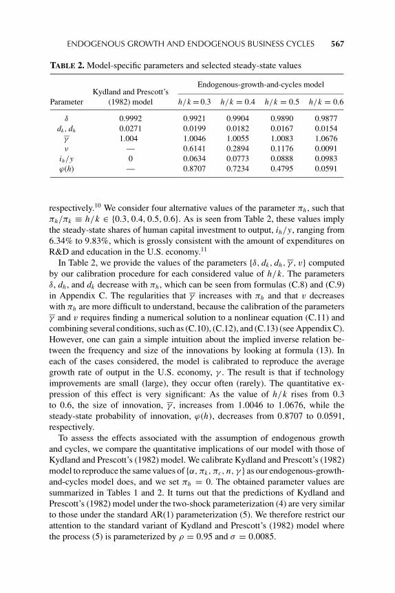
TABLE 2. Model-specific parameters and selected steady-state values

Endogenous-growth-and-cycles modelKydland and Prescott’s

Parameter (1982) model h/k = 0.3 h/k = 0.4 h/k = 0.5 h/k = 0.6

δ 0.9992 0.9921 0.9904 0.9890 0.9877dk, dh 0.0271 0.0199 0.0182 0.0167 0.0154

γ 1.004 1.0046 1.0055 1.0083 1.0676ν — 0.6141 0.2894 0.1176 0.0091

ih/y 0 0.0634 0.0773 0.0888 0.0983ϕ(h) — 0.8707 0.7234 0.4795 0.0591

respectively.10 We consider four alternative values of the parameter πh, such thatπh/πk ≡ h/k ∈ {0.3, 0.4, 0.5, 0.6}. As is seen from Table 2, these values implythe steady-state shares of human capital investment to output, ih/y, ranging from6.34% to 9.83%, which is grossly consistent with the amount of expenditures onR&D and education in the U.S. economy.11

In Table 2, we provide the values of the parameters {δ, dk, dh, γ , v} computedby our calibration procedure for each considered value of h/k. The parametersδ, dh, and dk decrease with πh, which can be seen from formulas (C.8) and (C.9)in Appendix C. The regularities that γ increases with πh and that v decreaseswith πh are more difficult to understand, because the calibration of the parametersγ and v requires finding a numerical solution to a nonlinear equation (C.11) andcombining several conditions, such as (C.10), (C.12), and (C.13) (see Appendix C).However, one can gain a simple intuition about the implied inverse relation be-tween the frequency and size of the innovations by looking at formula (13). Ineach of the cases considered, the model is calibrated to reproduce the averagegrowth rate of output in the U.S. economy, γ . The result is that if technologyimprovements are small (large), they occur often (rarely). The quantitative ex-pression of this effect is very significant: As the value of h/k rises from 0.3to 0.6, the size of innovation, γ , increases from 1.0046 to 1.0676, while thesteady-state probability of innovation, ϕ(h), decreases from 0.8707 to 0.0591,respectively.

To assess the effects associated with the assumption of endogenous growthand cycles, we compare the quantitative implications of our model with those ofKydland and Prescott’s (1982) model. We calibrate Kydland and Prescott’s (1982)model to reproduce the same values of {α, πk, πc, n, γ } as our endogenous-growth-and-cycles model does, and we set πh = 0. The obtained parameter values aresummarized in Tables 1 and 2. It turns out that the predictions of Kydland andPrescott’s (1982) model under the two-shock parameterization (4) are very similarto those under the standard AR(1) parameterization (5). We therefore restrict ourattention to the standard variant of Kydland and Prescott’s (1982) model wherethe process (5) is parameterized by ρ = 0.95 and σ = 0.0085.


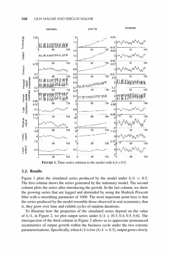
FIGURE 1. Time-series solution to the model with h/k = 0.5.

3.2. Results

Figure 1 plots the simulated series produced by the model under h/k = 0.5.The first column shows the series generated by the stationary model. The secondcolumn plots the series after introducing the growth. In the last column, we showthe growing series that are logged and detrended by using the Hodrick-Prescottfilter with a smoothing parameter of 1600. The most important point here is thatthe series produced by the model resemble those observed in real economies; thatis, they grow over time and exhibit cycles of random durations.

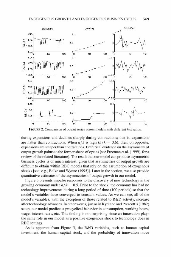
To illustrate how the properties of the simulated series depend on the valueof h/k, in Figure 2, we plot output series under h/k ∈ {0.3, 0.4, 0.5, 0.6}. Theintrospection of the third column in Figure 2 allows us to appreciate pronouncedasymmetries of output growth within the business cycle under the two extremeparameterizations. Specifically, when h/k is low (h/k = 0.3), output grows slowly


FIGURE 2. Comparison of output series across models with different h/k ratios.

during expansions and declines sharply during contractions; that is, expansionsare flatter than contractions. When h/k is high (h/k = 0.6), then, on opposite,expansions are steeper than contractions. Empirical evidence on the asymmetry ofoutput growth points to the former shape of cycles [see Freeman et al. (1999), for areview of the related literature]. The result that our model can produce asymmetricbusiness cycles is of much interest, given that asymmetries of output growth aredifficult to obtain within RBC models that rely on the assumption of exogenousshocks [see, e.g., Balke and Wynne (1995)]. Later in the section, we also providequantitative estimates of the asymmetries of output growth in our model.

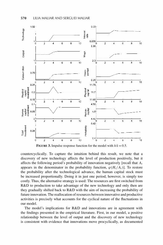
Figure 3 presents impulse responses to the discovery of new technology in thegrowing economy under h/k = 0.5. Prior to the shock, the economy has had notechnology improvements during a long period of time (100 periods) so that themodel’s variables have converged to constant values. As we can see, all of themodel’s variables, with the exception of those related to R&D activity, increaseafter technology advances. In other words, just as in Kydland and Prescott’s (1982)setup, our model predicts a procyclical behavior in consumption, working hours,wage, interest rates, etc. This finding is not surprising since an innovation playsthe same role in our model as a positive exogenous shock to technology does inRBC settings.

As is apparent from Figure 3, the R&D variables, such as human capitalinvestment, the human capital stock, and the probability of innovation move


FIGURE 3. Impulse response function for the model with h/k = 0.5.

countercyclically. To capture the intuition behind this result, we note that adiscovery of new technology affects the level of production positively, but itaffects the following period’s probability of innovation negatively [recall that At

appears in the denominator in the probability function, ϕ(Ht/At)]. To restorethe probability after the technological advance, the human capital stock mustbe increased proportionally. Doing it in just one period, however, is simply toocostly. Thus, the alternative strategy is used: The resources are first switched fromR&D to production to take advantage of the new technology and only then arethey gradually shifted back to R&D with the aim of increasing the probability offuture innovation. The reallocation of resources between innovative and productiveactivities is precisely what accounts for the cyclical nature of the fluctuations inour model.

The model’s implications for R&D and innovations are in agreement withthe findings presented in the empirical literature. First, in our model, a positiverelationship between the level of output and the discovery of new technologyis consistent with evidence that innovations move procyclically, as documented


TABLE 3. Selected second moments for the U.S. and artificial economiesa

Kydland and Endogenous-growth-and-cycles modelPrescott’s U.S.

Statistica (1982) model h/k = 0.3 h/k = 0.4 h/k = 0.5 h/k = 0.6 economy

σA/σ y — 1.139 1.099 1.030 0.982 —(0.009) (0.008) (0.014) (0.018)

σϕ /σ y — 0.290 0.717 1.660 2.457 —(0.023) (0.024) (0.030) (0.066)

σ c/σ y 0.302 0.444 0.462 0.534 0.559 0.511(0.014) (0.009) (0.007) (0.007) (0.007)

σ i /σ y 2.507 2.205 2.206 2.165 2.129 2.864(0.032) (0.015) (0.020) (0.034) (0.032)

σn/σ y 0.513 0.402 0.387 0.343 0.331 0.769(0.005) (0.005) (0.005) (0.007) (0.005)

σw/σ y 0.505 0.610 0.622 0.668 0.685 0.611(0.008) (0.006) (0.005) (0.005) (0.004)

σ y 1.636 0.184 0.301 0.492 1.619 1.676(0.170) (0.023) (0.030) (0.053) (0.321)

corr(At, yt ) 0.999 0.999 0.998 0.984 0.971 —(0.000) (0.004) (0.005) (0.006) (0.007)

corr(ϕt+1, yt ) — −0.983 −0.980 −0.959 −0.943 —(0.018) (0.013) (0.009) (0.009)

corr(ct , yt ) 0.892 0.969 0.980 0.983 0.977 0.846(0.018) (0.007) (0.007) (0.007) (0.005)

corr(it , yt ) 0.993 0.995 0.996 0.994 0.991 0.914(0.002) (0.001) (0.001) (0.003) (0.003)

corr(nt , yt ) 0.983 0.982 0.986 0.980 0.968 0.899(0.004) (0.004) (0.004) (0.005) (0.007)

corr(wt, yt ) 0.982 0.992 0.995 0.995 0.993 0.464(0.004) (0.002) (0.002) (0.002) (0.002)

corr(wt, nt ) 0.931 0.951 0.963 0.953 0.930 0.219(0.016) (0.011) (0.011) (0.014) (0.015)

a Statistics σx and corr(x, z) are the volatility of a variable x and the correlation coefficient between variables x andz, respectively. The volatilities and the correlation coefficients of the models’ variables are sample averages across500 simulations. Each simulation consists of 157 periods, as do the U.S. time series. Numbers in parentheses are thesample standard deviations of the corresponding statistics. Before calculating any statistic, we log all the variablesfor the U.S. and artificial economies and detrend them by using the Hodrick-Prescott filter with a penalty parameterof 1600.

by Geroski and Walters (1995). Second, the countercyclical pattern of the R&Dactivity produced by the model agrees with the findings of Lach and Schankerman(1989) and Lach and Rob (1996), who show that an increase in R&D investmentprecedes an expansion in physical capital investment.

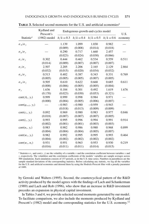
In Tables 3 and 4, we provide selected second moments generated by our model.To facilitate comparison, we also include the moments produced by Kydland andPrescott’s (1982) model and the corresponding statistics for the U.S. economy.12


TABLE 4. Autocorrelation coefficients for output and output growth and theskewness coefficients for the first difference of output for the U.S. and artificialeconomiesa

Kydland and Endogenous-growth-and cycles modelPrescott’s U.S.

Statistic (1982) model h/k = 0.3 h/k = 0.4 h/k = 0.5 h/k = 0.6 economy

corr(yt , yt−1) 0.696 0.682 0.723 0.787 0.810 0.867(0.056) (0.063) (0.055) (0.043) (0.032)

corr(yt , yt−2) 0.446 0.441 0.464 0.499 0.513 0.681(0.088) (0.094) (0.091) (0.088) (0.074)

corr(yt , yt−3) 0.245 0.242 0.257 0.271 0.275 0.470(0.103) (0.105) (0.108) (0.107) (0.096)

corr(yt , yt−4) 0.082 0.083 0.092 0.091 0.090 0.258(0.113) (0.110) (0.111) (0.115) (0.107)

corr(yt , yt−5) −0.044 −0.040 −0.033 −0.045 −0.049 0.042(0.111) (0.106) (0.109) (0.115) (0.111)

skew(yt − yt−1) −0.0193 −1.8645 −0.6427 0.4768 3.7151 −0.1904(0.1962) (0.3438) (0.2455) (0.2426) (0.8199)

corr(γ t ,γ t−1) −0.020 −0.044 0.049 0.261 0.356 0.290(0.077) (0.078) (0.082) (0.072) (0.060)

corr(γ t ,γ t−2) −0.018 −0.001 −0.011 −0.019 −0.029 0.189(0.074) (0.080) (0.079) (0.090) (0.087)

corr(γ t ,γ t−3) −0.017 −0.003 −0.003 −0.015 −0.020 0.084(0.078) (0.081) (0.089) (0.090) (0.083)

corr(γ t ,γ t−4) −0.017 −0.004 −0.009 −0.014 −0.016 0.053(0.079) (0.081) (0.082) (0.088) (0.091)

corr(γ t ,γ t−5) −0.019 −0.010 −0.008 −0.018 −0.016 −0.108(0.078) (0.086) (0.083) (0.087) (0.090)

a Statistics corr(x, z) and skew(x) are the correlation coefficient between variables x and z, and the skewnesscoefficient of a variable x, respectively. The correlation and skewness coefficients of the models’ variables are sampleaverages across 500 simulations. Each simulation consists of 157 periods, as do the U.S. time series. Numbers inparentheses are the sample standard deviations of the corresponding statistics. Before calculating any statistic, welog all the variables for the U.S. and artificial economies and detrend them by using the Hodrick-Prescott filter witha penalty parameter of 1600.

Before computing the second moments, we remove the growth in a way that isstandard in the RBC literature: We log all the variables for the U.S and artificialeconomies and detrend them by using the Hodrick-Prescott filter with a penaltyparameter of 1600.13

The main findings in Table 3 are as follows: Overall, the relative volatilities andcontemporaneous correlations in our model are close to the respective statisticsin Kydland and Prescott’s (1982) setup. The volatility of output in our model isdetermined by the size of technological advance and increases from 0.18 to 1.62as the value of h/k rises from 0.3 to 0.6 (note that the volatility of output in thelatter case is comparable to the one in the data, 1.64). The correlation between the


current output and the next period’s probability of innovation, ϕt+1 ≡ ϕ(Ht/At),is negative and close to perfect (recall that a countercyclical movement of R&Dactivity accounts for the cycles in our model).

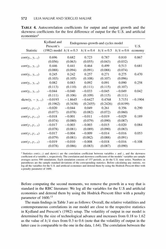
As is seen from Table 4, our model is capable of delivering fluctuations in thebusiness-cycle frequency. Indeed, the autocorrelation coefficients of output at shortlags in our model are close to those of the U.S. economy and practically identicalto those presented in Kydland and Prescott’s (1982) model. A realistic persistenceof output in an RBC model is a consequence of assuming an exogenous AR(1)technological shock with the required degree of serial correlation. In contrast, ourendogenous-growth-and-cycles model can produce an appropriate cyclical patternof output without having any exogenous source of technological persistence. Thisfinding is interesting since the existing models for endogenous cycles do notproduce business-cycle fluctuations [see Andolfatto and MacDonald (1998) andFreeman et al. (1999)].

To quantify the asymmetries of output growth in our model, we compute theskewness coefficient for the first difference of detrended output, as is suggestedby Sichel (1993). If expansions are steeper than contractions, then the suddendecreases in the output series should be larger, but more rare, than the mildincreases in this series, so that the first difference of output should display negativeskewness. As we see from Table 4, the skewness coefficient that we obtained fromthe U.S. output series is negative and equal to −0.19. In Kydland and Prescott’s(1982) model, this coefficient is nearly zero, which means that the cycles aresymmetric. Our model is capable of generating a wide range for the skewnesscoefficient from a large negative (−1.8645) under h/k = 0.3 to a large positive(3.7151) under h/k = 0.6. In particular, it is clear that under some value ofh/k ∈ (0.4, 0.5), our model can generate the skewness coefficient that is equal tothe empirical counterpart.

We finally discuss the implications our model has for persistence in outputgrowth. It is a stylized fact that U.S. output growth displays significant positiveautocorrelations over short horizons and weak negative autocorrelations over longhorizons [see Cogley and Nason (1995) for a detailed discussion]. To illustratethe quantitative expression of this tendency in our data set, in the last column ofTable 4, we provide the autocorrelations for output growth, γt ≡ yt/yt−1, at thefirst five lags. Kydland and Prescott’s (1982) model cannot account for the abovestylized fact: It generates weak negative autocorrelations at the five lags considered[see the first column of Table 4)].14 The failure of Kydland and Prescott’s (1982)model in this dimension is explained by a weakness of the embodied propagationmechanisms, which are capital accumulation and intertemporal substitution. In ourmodel, the presence of human capital gives rise to an additional propagation mech-anism: A discovery of new technology triggers the reallocation of resources fromR&D activities to production, which increases the future output. As can be seenfrom Table 4, under high values of h/k ∈ {0.5, 0.6}, this mechanism is so strongthat our model is able to generate the first-order autocorrelation of output growth,which is close to the one observed in the U.S. data. Thus, our model of endogenous


growth and cycles generates more realistic output dynamics than does the standardRBC model.

4. CONCLUSION

Models with endogenous innovations have been previously applied in an attemptto explain long waves in economic activity. The theoretical and empirical resultsof this paper provide support for the hypothesis that innovations also play animportant role in business cycles. We construct an R&D-based general equilibriummodel in which both the long-run growth and the short-run cyclical fluctuationsarise endogenously because of continuous technological progress. In our economy,three factors that affect the outcome of R&D activity are research efforts, theexisting stock of knowledge, and a random component. The calibrated version ofour endogenous-growth-and-cycles model has proved to be as good in reproducingthe business-cycle facts as the benchmark RBC setup by Kydland and Prescott(1982). Furthermore, our model can account for two stylized facts that cannot bereconciled within the typical RBC model, such as the asymmetry in the shape ofbusiness cycles and the persistence in output growth.

NOTES

1. For example, this idea lies in the basis of the models developed by Aghion and Howitt (1992),Grossman and Helpman (1991), Romer (1990), and Segerstrom (1991).

2. In Andolfatto and MacDonald (1998), there is idiosyncratic uncertainty but not aggregate un-certainty; this is because a continuum of agents is assumed and thus the law of large numbers applies.In Freeman et al. (1999), uncertainty is absent: innovation occurs with the probability 1 as soon as therequired amounts of R&D resources have been collected.

3. Jovanovic and Rob (1990) provide many examples of research projects that have had randomoutcomes.

4. There is evidence that supports the two-regime process assumption. Hamilton (1989) finds thatthe periodic shifts between positive and negative growth in output concur remarkably with the datesof expansions and recessions in the U.S. economy.

5. A related idea appears in Jovanovic and Lach (1997, p. 7) in a context of a product-innovationmodel: “ more important products are the embodiment of a larger number of innovations, so that, forexample, the computer embodies a large ‘bunch’ of smaller innovations.”

6. Thus, production technology follows a random-walk type of process. In At = ln At−1 +ln γt , γt ∈ {γ , 1}, where the probabilities of the two states, ϕt and (1 − ϕt ), change over time.The assumption of a random-walk process for innovations is in agreement with the data [see Geroskiand Walters (1995)].

7. Consequently, our model reproduces empirical evidence that indicates that real economiesconstantly increase their spending on R&D, although their growth rates change relatively little. Thisevidence is documented by Coe and Helpman (1995), Griliches (1988), Grossman and Helpman (1991,Table 1.1), Jones (1995), and Kortum (1997), among others. Jones (1995) argues that such evidencecannot be replicated under the assumption of constant returns to R&D activity that is standard forR&D-based models; see, for example, Aghion and Howitt (1992), Grossman and Helpman (1991),and Romer (1990).

8. The standard transformation for removing the growth in Kydland and Prescott’s (1982) modelis ct ≡ Ct/Xt and kt ≡ Kt/Xt . The objective function obtained after this transformation contains the


growing term Xt . However, in contrast to our model, the growing term in this case is exogenous anddoes not affect the equilibrium allocation.

9. Here, and further on in the text, z denotes the steady-state value of a variable zt .10. World Bank’s Web site (http://www.worldbank.org/), Tables 5.15 and 2.9, respectively.11. The estimates of McGrattan and Prescott (2000) offer an alternative justification for the assumed

range of h/k. This paper reports a ratio of approximately 0.6 between what they call unmeasured andmeasured corporate capital, with the former kind of capital being defined as brand names, patents, andfirm-specific human capital.

12. See Maliar and Maliar (2003a) for a description of the U.S. time-series data that were used togenerate the empirical statistics in Tables 3 and 4.

13. We focus exclusively on the second-moments properties of the original nonstationary models.The first moments (levels) generated by the supplementary stationary models are not reported becausesuch models have no clear economic interpretation.

14. Cogley and Nason (1995) show that other standard RBC models [e.g., Hansen’s (1985) modelwith indivisible labor, Christiano and Eichenbaum’s (1992) model with government spending shocks)also have difficulties in generating the appropriate dynamics of output growth.

15. We find that using a more accurate second-order polynomial approximation for the decisionrules instead of the first-order one affects the solution very little but raises the computational expensessignificantly.

REFERENCES

Aghion, P. & P. Howitt (1992) A model of growth through creative destruction. Econometrica 60,323–351.

Andolfatto, D. & G. MacDonald (1998) Technology diffusion and aggregate dynamics. Review ofEconomic Dynamics 1, 338–370.

Balke, N. & M. Wynne (1995) Recessions and recoveries in real business cycle models. EconomicInquiry 33, 640–663.

Bental, B. & D. Peled (1996) The accumulation of wealth and the cyclical generation of new technolo-gies: A search theoretic approach. International Economic Review 37, 687–718.

Christiano, L. & M. Eichenbaum (1992) Current real-business-cycle theories and aggregate labor-market fluctuations. American Economic Review 82, 430–450.

Coe, D. & E. Helpman (1995) International R&D spillovers. European Economic Review 39,859–887.

Cogley, T. & J. Nason (1995) Output dynamics in real-business-cycle models. American EconomicReview 85, 492–511.

Den Haan, W. & A. Marcet (1990) Solving the stochastic growth model by parametrizing expectations.Journal of Business and Economic Statistics 8, 31–34.

Freeman, S., D.–P. Hong & D. Peled (1999) Endogenous cycles and growth with indivisible techno-logical developments. Review of Economic Dynamics 2, 403–433.

Geroski, P. & C. Walters (1995) Innovative activity over the business cycle. Economic Journal 1005,916–928.

Griliches, Z. (1988) Productivity puzzles and R&D: Another nonexplanation. Journal of EconomicPerspectives 2, 9–21.

Grossmann, G. & E. Helpman (1991) Innovation and Growth in the Global Economy. Cambridge,MA: MIT Press.

Hamilton, J. (1989) A new approach to the economic analysis of nonstationary time series and thebusiness cycle. Econometrica 57, 357–384.

Hansen, G. (1985) Indivisible labor and the business cycle. Journal of Monetary Economics 16,309–328.

Jones, C. (1995) Time series tests of endogenous growth models. Quarterly Journal of Economics 110,495–525.


Jovanovic, B. & S. Lach (1997) Product innovation and the business cycle. International EconomicReview 1, 3–22.

Jovanovic, B. & R. Rob (1990) Long waves and short waves: Growth through intensive and extensivesearch. Econometrica 58, 1391–1409.

Juster, F. & F. Stafford (1991) The allocation of time: Empirical findings, behavioral models, andproblems of measurement. Journal of Economic Literature 29, 471–522.

Kleinknecht, A. (1987) Innovation Patterns in Crisis and Prosperity: Schumpeter’s Long Cycle Re-considered. London: Macmillan.

Kortum, S. (1997) Research, patenting, and technological change. Econometrica 6, 1389–1419.Kydland, F. & E. Prescott (1982) Time to build and aggregate fluctuations. Econometrica 50, 1345–

1370.Lach, S. & R. Rob (1996) R&D, investment and industry dynamics. Journal of Economics and

Management Strategy 2, 217–249.Lach, S. & M. Schankerman (1989) Dynamics of R&D and investment in the scientific sector. Journal

of Political Economy 4, 880–904.Maliar, L. & S. Maliar (2003a) The representative consumer in the neoclassical growth model with

idiosyncratic shocks. Review of Economic Dynamics 6, 362–380.Maliar, L. & S. Maliar (2003b) Parameterized expectations algorithm and the moving bounds. Journal

of Business and Economic Statistics 21, 88–92.Marcet, A. & G. Lorenzoni (1999) The parameterized expectations approach: Some practical issues.

In R. Marimon & A. Scott (eds.), Computational Methods for the Study of Dynamic Economies,pp. 143–172. Oxford: Oxford University Press.

McGrattan, E. & E. Prescott (2000) Is the stock market overvalued? Minneapolis Federal ReserveBank. Quarterly Review 24(4), 20–40.

Romer, P. (1990) Endogenous technical change. Journal of Political Economy 98, S71–S103.Segerstrom, P. (1991) Innovation, imitation, and economic growth. Journal of Political Economy 99,

807–827.Sichel, D. (1993) Business cycle asymmetry: A deeper look. Economic Inquiry 31, 224–236.

APPENDIX A: DECENTRALIZATION OFTHE PLANNER’S ECONOMY

A market economy consists of one production firm, one research firm, and a continuum ofhomogeneous agents with the names on the unit interval [0, 1].

A research firm rents the human capital stock, accumulated by the agents. In ex-change for the supplied human capital, Ht−1, an agent receives a new technology withthe probability ϕt = ϕ(Ht−1/At−1). Because all agents are identical, in the equilibrium,the individual human capital stock coincides with the aggregate one. Thus, when thenew technology, At , is discovered, the research firm delivers it to all agents in theeconomy.

Except for human capital, an agent accumulates physical capital and rents it to theproduction firm at the interest rate, rt . Also, the agent supplies efficiency labor in exchangefor the wage, wt . The problem of the agent is

max{Ct ,lt ,Kt ,Ht }∞t=0

E0

∞∑t=0

δt {ln Ct + B ln lt }


subject to

Ct + Kt + Ht = (1 − dk + rt )Kt−1 + (1 − dh)Ht−1 + wtAt (1 − lt ),

where At represents the efficiency of 1 hour worked, that is, the current level of technology.The production firm maximizes period-by-period profit by choosing the demand for

physical capital and efficiency labor. In the equilibrium, the marginal product of each inputis equal to its rental price

rt = αKα−1t−1 [At(1 − lt )]

1−α = αγ 1−αt kα−1

t−1 (1 − lt )1−α,

wt = (1 − α)Kαt−1[At(1 − lt )]

−α = (1 − α)γ 1−αt kα

t−1(1 − lt )−α.

The fact that the planner’s economy and the market economy have an identical optimalallocation follows from the equivalence of the optimality conditions.

APPENDIX B: PROOF OF PROPOSITION 1

(a) Let Wt be the value of lifetime utility in period t . From (6), we have

Wt = ln ct + B ln lt + ln At−1 + δEt

[ ∞∑s=0

δs(ln ct+1+s + B ln lt+1+s + ln At+s )

].

The value function Wt varies with time as it depends on the growing-over-time technologyAt−1. We guess that the function Wt can be represented as Wt = V (kt−1, ht−1, γt )+µ ln At−1,where V is a time-invariant value function, which depends on the endogenous state variableskt−1, ht−1 and the exogenous state variable γt . Then, we obtain

V (kt−1, ht−1, γt ) = Wt − µ ln At−1 = ln ct + B ln lt + ln At−1 − µ ln At−1

+ δEt

[ ∞∑s=0


]= ln ct + B ln lt + δµ ln At

− δµ ln At + (1 − µ) ln At−1 + δEt

[ ∞∑s=0


].

By using the fact that ln At = ln At−1 + ln γt , we get

V (kt−1, ht−1, γt ) = ln ct + B ln lt + (1 − µ + δµ) ln At−1 + δµ ln γt

+ δEt

∞∑s=0

[δs(ln ct+1+s + B ln lt+1+s + ln At+s ) − µ ln At ] = ln ct + B ln lt

+ (1 − µ + δµ) ln At−1 + δµ ln γt + δEt [(Wt+1 − µ ln At)] = ln ct + B ln lt

+ (1 − µ + δµ) ln At−1 + δµ ln γt + δEt [V (kt , ht , γt+1)] .


In order V (kt , ht , γt+1) is time-invariant, the term ln At−1 should disappear from the lastequation. This implies that (1 − µ + δµ) = 0. Consequently, we have

V (kt−1, ht−1, γt ) = ln ct + B ln lt + δ

1 − δln γt + δEt [V (kt , ht , γt+1)].

This functional equation is equivalent to the Bellman equation (9).(b) We define the operator

TV = maxlt ,kt ,ht

{ut + δϕ(ht )V (kt , ht , γ ) + δ [1 − ϕ(ht )] V (kt , ht , 1)},

where ut = u(kt−1, ht−1, γt , kt , ht , lt ) represents the momentary utility of period t aftersubstituting consumption from budget constraint (7).

To show that T is a contraction, we verify that it satisfies Blackwell’s sufficiencyconditions.

First, suppose kt−1 ∈K≡ [kmin, kmax], ht−1 ∈H≡ [hmin, hmax] and lt ∈ [0, 1]. Con-sider any two functions f and φ, defined on K×H× {γ , 1}. Assume that f (kt−1,

ht−1, γt ) ≥φ(kt−1, ht−1, γt ) for all kt−1 ∈K, ht−1 ∈H, γt ∈ {γ , 1}. Let (kft , h

ft , l

ft ) and

(kφt , h

φt , l

φt ) attain Tf and T φ, respectively, for any kt−1 ∈K, ht−1 ∈H, γt ∈ {γ , 1}. After

denoting uft = u(kt−1, ht−1, γt , k

ft , h

ft , l

ft ) and u

φt = u(kt−1, ht−1, γt , k

φt , h

φt , l

φt ), we have

Tf = uft + δϕ

(h

ft

)f(k

ft , h

ft , γ

)+ δ

[1 − ϕ

(h

ft

)]f(k

ft , h

ft , 1

)≥ u

φt + δϕ

(h

φt

)f(k

φt , h

φt , γ

)+ δ

[1 − ϕ

(h

φt

)]f(k

φt , h

φt , 1

)≥ u

φt + δϕ

(h

φt

)φ(k

φt , h

φt , γ

)+ δ

[1 − ϕ

(h

φt

)]φ(k

φt , h

φt , 1

)= T φ.

Therefore, T is monotone.Second, for any positive constant m ≥ 0, we obtain

T (V + m) = maxlt ,kt ,ht

{ut + δϕ(ht ) [V (kt , ht , γ ) + m]

+ δ [1 − ϕ(ht )] · [V (kt , ht , 1) + m]} = TV + δm.

Therefore, T discounts.

APPENDIX C: CALIBRATIONPROCEDURE

We calibrate the parameters of the model in the steady state. We define a steady state asa situation in which all variables of the stationary economy (6)–(8) take constant values.In the steady state, instead of switching between two different growth rates, γt ∈ {γ , 1}and, consequently, two levels of labor productivity, γ 1−α

t ∈ {γ 1−α, 1}, the economy faces aconstant growth rate, γ , and a constant level of labor productivity, a, given by

γ = γ ϕ(h) + 1 − ϕ(h), (C.1)

a = γ 1−αϕ(h) + 1 − ϕ(h). (C.2)


By evaluating FOCs (10)–(12) and constraint (7) in the steady state, we obtain, respectively,

c = (1 − α)l

Ba kαn−α, (C.3)

γ

δ= 1 − dk + αa kα−1n1−α, (C.4)

γ

δ= 1 − dh + v exp(−vh)cδ ln γ

1 − δ, (C.5)

c + γ (k + h) = (1 − dk)k + (1 − dh)h + a kαn1−α, (C.6)

where n = 1 − l. In terms of the ratios πc, πk , and πh, conditions (C.3), (C.4), and (C.6)can be rewritten as

B = πcn

(1 − n)(1 − α), (C.7)

δ = γ

1 − dk + α/πk

, (C.8)

dk = dh = 1 − γ + 1 − πc

πh + πk

. (C.9)

Equations (C.7)–(C.9) provide a basis for calibrating the parameters B, δ, dk , and dh.We now calibrate the parameter γ . From (C.1) we have that exp(−vh) = 1 − ϕ(h) =

(γ − γ )/(γ − 1) and, consequently,

v = − 1

hln

(γ − γ

γ − 1

). (C.10)

The last result allows us to rewrite condition (18) as follows:

γ

δ= 1 − dh − πc

πh

(γ − γ

γ − 1

)ln

(γ − γ

γ − 1

)· δ ln γ

1 − δ. (C.11)

By solving this equation numerically, we obtain the value of the parameter γ . Next, werestore the technology by using (C.2)

a = γ 1−α

(γ − 1

γ − 1

)+

(γ − γ

γ − 1

). (C.12)

Given the technology level, we compute the capital-to-labor ratio,

k

n=

[γ /δ − 1 + dk

αa

]1/(α−1)

, (C.13)

and find the steady-state level of output, y = an(k/n)α . Subsequently, we compute thesteady-state human capital stock, h = πhy, and calibrate the parameter v by using equa-tion (23).

In sum, our calibration procedure identifies uniquely the model’s parameters{B, δ, dk, dh, γ , v} so that the model reproduces {πc, πk, πh, n, γ }.


The steady-state expression of the FOCs of Kydland and Prescott’s (1982) model coin-cides with (C.7)–(C.9) under πh = 0. For given {πc, πk, n, γ }, these conditions identify thevalues of B, δ, and dk .

APPENDIX D: SOLUTION PROCEDURE

To solve for equilibrium in the model, we employ a variant of the parameterized expectationsalgorithm (PEA) by Den Haan and Marcet (1990). A further description of the PEA andits applications can be found in Marcet and Lorenzoni (1999). To ensure the convergenceof the PEA, we bound the simulated series on initial iterations as described in Maliar andMaliar (2003b).

Since there are two intertemporal FOCs, we must parameterize two conditional expec-tations. We parameterize the right-hand side of FOC (11) as follows:15

γtct

δ= exp(β1 + β2 ln kt−1 + β3 ln ht−1 + β4 ln γt ). (D.1)

The second intertemporal FOC may not be parameterized in this manner because therewould be two equations identifying consumption and no condition identifying physical andhuman capital. To deal with this complication, we premultiply both sides of FOC (12) byht and parameterize the right-hand side of the resulting condition as follows:

γtct

δ· ht = exp(λ1 + λ2 ln kt−1 + λ3 ln ht−1 + λ4 ln γt ). (D.2)

We approximate the optimal value function V (kt−1, ht−1, γt ) by a second-order polynomial

V(kt−1, ht−1, γt ) = η1 + η2 ln kt−1 + η3 ln ht−1 + η4 ln γt + η5 ln kt−1 ln ht−1

+ η6 ln kt−1 ln γt + η7 ln ht−1 ln γt + η8(ln kt−1)2 + η9(ln ht−1)

2 + η10(ln γt )2. (D.3)

We use the following iterative procedure:

• Step 1. Fix the initial coefficients {βi}4i=1, {λi}4

i=1 and {ηi}10i=1. Fix initial condition

(k−1, h−1). Draw a random series of numbers {ut }Tt=0 from a uniform distribution,

[0, 1], and fix it.• Step 2. Given {βi}4

i=1 and {λi}4i=1, use (7), (10), (27), and (28) to calculate recursively

{cg

t+1, cbt+1, l

g

t+1, lbt+1, kt , ht , γt }T

t=0. To determine a sequence of the economy’s states,use the series {ut }T

t=0. Specifically, for each t , compute the probability ϕ(ht ) andcompare it with the random number ut . If ϕ(ht )≥ ut , then assume γt = γ ; otherwise,take γt = 1.

• Step 3. Given {ηi}10i=1 and {cg

t+1, cbt+1, l

g

t+1, lbt+1, kt , ht , γt }T

t=0, from the Bellman equa-tion (9), compute the series of values of the value function in the two states,{V (kt−1, ht−1, γt ), V (kt−1, ht−1, 1)}T

t=0. Restore the variables in the right-hand sidesof FOCs (11) and (12). Run the nonlinear least-square regressions of the correspond-ing variables on the functional forms (D.1), (D.2), and (D.3). Use the reestimatedcoefficients {βi}4

i=1, {λi}4i=1 and {ηi}10

i=1 as input for next iteration.


Iterate on the coefficients {βi}4i=1, {λi}4

i=1, and {ηi}10i=1 until a fixed point is found. To

solve for a fixed point, we use a built-in MATLAB gradient-descent procedure “f solve.”The length of simulations was T = 5,000.

We also apply the PEA for calculating a solution to Kydland and Prescott’s (1982)model. We parameterize the intertemporal condition of the stationary version of the modelas follows:

γ ct

δ= exp(e1 + e2 ln kt−1 + e3 ln θt ).

We fix initial condition (k−1, θ−1) and the initial coefficients {ei}3i=1. We draw a series of

technology shocks, {θt }Tt=1, and fix it. As above, we iterate on the coefficients {ei}3

i=1 untilwe find a fixed point.

ENDOGENOUS GROWTH AND ENDOGENOUS BUSINESS CYCLESmaliarl/Files/MD2004.pdf · ENDOGENOUS GROWTH AND...

Documents

Transcript of ENDOGENOUS GROWTH AND ENDOGENOUS BUSINESS CYCLESmaliarl/Files/MD2004.pdf · ENDOGENOUS GROWTH AND...