Endogenous Ranking and Equilibrium Lorenz …faculty.wcas.northwestern.edu/~kmatsu/Endogenous...

Endogenous Ranking and Equilibrium Lorenz Curve Across (ex-ante) Identical Countries

By Kiminori Matsuyama1

January 2013

Abstract: This paper proposes a symmetry-breaking model of trade with a (large but) finite number of (ex-ante) identical countries and a continuum of tradeable goods, which differ in their dependence on local differentiated producer services. Productivity differences across countries arise endogenously through free entry to the local service sector in each country. In any stable equilibrium, the countries sort themselves into specializing in different sets of tradeable goods and a strict ranking of countries in per capita income, TFP, and the capital-labor ratio emerge endogenously. Furthermore, the distribution of country shares, the Lorenz curve, is unique and analytically solvable in the limit, as the number of countries grows unbounded. Using this limit as an approximation allows us to study what determines the shape of distribution, perform various comparative statics and to evaluate the welfare effects of trade. Keywords: Endogenous Comparative Advantage, Endogenous Dispersion, Globalization and Inequality, Symmetry-Breaking, Lorenz-dominant shifts, Log-submodularity JEL Classification Numbers: F12, F43, O11, O19

1 Email: [email protected]; Homepage: http://faculty.wcas.northwestern.edu/~kmatsu/. Some of the results here have previously been circulated as a memo entitled “Emergent International Economic Order.” I am grateful to conference and seminar participants at Bocconi/IGIER, Bologna, Chicago, Columbia, CREI/Pompeu Fabra, Harvard, Hitotsubashi, Keio/GSEC, Kyoto, three different groups of NBER Summer Institute, NYU, Princeton, Tokyo, and Urbino for their feedback. I also benefited greatly from the discussion with Hiroshi Matano on the approximation method used in the paper. Detailed comments and suggestions by the editor and the referees have greatly improved the paper.

©Kiminori Matsuyama, Endogenous Ranking and Equilibrium Lorenz Curve

- 1 -

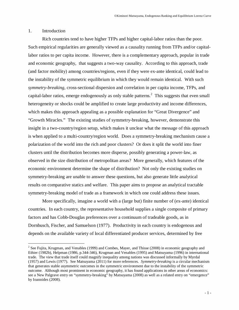
1. Introduction

Rich countries tend to have higher TFPs and higher capital-labor ratios than the poor.

Such empirical regularities are generally viewed as a causality running from TFPs and/or capital-

labor ratios to per capita income. However, there is a complementary approach, popular in trade

and economic geography, that suggests a two-way causality. According to this approach, trade

(and factor mobility) among countries/regions, even if they were ex-ante identical, could lead to

the instability of the symmetric equilibrium in which they would remain identical. With such

symmetry-breaking, cross-sectional dispersion and correlation in per capita income, TFPs, and

capital-labor ratios, emerge endogenously as only stable patterns.2 This suggests that even small

heterogeneity or shocks could be amplified to create large productivity and income differences,

which makes this approach appealing as a possible explanation for “Great Divergence” and

“Growth Miracles.” The existing studies of symmetry-breaking, however, demonstrate this

insight in a two-country/region setup, which makes it unclear what the message of this approach

is when applied to a multi-country/region world. Does a symmetry-breaking mechanism cause a

polarization of the world into the rich and poor clusters? Or does it split the world into finer

clusters until the distribution becomes more disperse, possibly generating a power-law, as

observed in the size distribution of metropolitan areas? More generally, which features of the

economic environment determine the shape of distribution? Not only the existing studies on

symmetry-breaking are unable to answer these questions, but also generate little analytical

results on comparative statics and welfare. This paper aims to propose an analytical tractable

symmetry-breaking model of trade as a framework in which one could address these issues.

More specifically, imagine a world with a (large but) finite number of (ex-ante) identical

countries. In each country, the representative household supplies a single composite of primary

factors and has Cobb-Douglas preferences over a continuum of tradeable goods, as in

Dornbusch, Fischer, and Samuelson (1977). Productivity in each country is endogenous and

depends on the available variety of local differentiated producer services, determined by free

2 See Fujita, Krugman, and Venables (1999) and Combes, Mayer, and Thisse (2008) in economic geography and Ethier (1982b), Helpman (1986, p.344-346), Krugman and Venables (1995) and Matsuyama (1996) in international trade. The view that trade itself could magnify inequality among nations was discussed informally by Myrdal (1957) and Lewis (1977). See Matsuyama (2011) for more references. Symmetry-breaking is a circular mechanism that generates stable asymmetric outcomes in the symmetric environment due to the instability of the symmetric outcome. Although most prominent in economic geography, it has found applications in other areas of economics: see a New Palgrave entry on “symmetry-breaking” by Matsuyama (2008) as well as a related entry on “emergence” by Ioannides (2008).


- 2 -

entry to the local service sector, as in Dixit and Stiglitz (1977) model of monopolistic

competition. One key assumption is that tradeable sectors differ in their dependence on local

services. This creates a circular mechanism between patterns of trade and cross-country

productivity differences. Having more variety of local services not only makes a country more

productive. It also gives a country comparative advantage in tradeable sectors that are more

dependent on those services. This in turn means a larger market for services, hence more firms

enter to provide such services. As a result, the country ends up having more variety of local

services and become more productive.

With (a continuum of) tradable goods vastly outnumbering (a finite number of) countries,

this circular mechanism sorts different countries into specializing in different sets of tradeable

goods (endogenous comparative advantage) and leads to a strict ranking of countries in income,

TFP, and (in an extension that allows for variable factor supply) capital-labor ratio in any stable

equilibrium. Furthermore, the equilibrium distribution of country shares, the Lorenz curve, is

unique and analytically tractable in the limit, as the number of countries grows unbounded.

Using this limit as an approximation allows us to study, among other things, what determines the

shape of distribution and how various forms of globalization or technical change affect

inequality across countries, and to evaluate the welfare effects of trade (e.g., when trade is

Pareto-improving, and when it is not, what fraction of countries might lose from trade).

Section 2.1 introduces the baseline model, which assumes that all consumption goods are

tradeable and all primary factors are in fixed supply. Section 2.2 derives a single-country (or

autarky) equilibrium. Section 2.3 derives a stable equilibrium with any finite number of

countries, whose associated Lorenz curve is characterized by the second-order difference

equation with two terminal conditions. Section 2.4 explains why any equilibrium in which some

countries remain identical ex-post is unstable. Section 2.5 shows that, as the number of countries

grows unbounded, the Lorenz curve converges to the solution of the second-order differential

equation with two terminal conditions, which is unique and analytically solvable. Armed with

the explicit formula for the limit Lorenz curve, this subsection shows when the distribution is

bimodal or satisfies a power-law. It also demonstrates that making local services more

differentiated causes a Lorenz-dominant shift of the distribution, leading to greater inequality

across countries. Section 2.6 studies the welfare effects of trade, which turns out to depend on

the heterogeneity of tradeable goods, measured by the Theil index of their dependence on local


- 3 -

services. Section 3 discusses two extensions. In section 3.1, a fraction of the consumption goods

are assumed to be nontradeable. This extension allows us to study the effects of globalization

through trade in goods. In section 3.2, one of the primary factors is allowed to vary in supply

either through factor mobility and accumulation. This extension not only generates the

correlation between the capital-labor ratio and per capita income and TFP, but also it allows us to

study the effects of technical change that increases the relative importance of human capital in

production and of globalization through factor mobility.

2. Baseline Model:

2.1 Key Elements of the Model

The world consists of J (ex-ante) identical countries, where J is a positive integer. There

may be multiple nontradeable primary factors of production, such as capital (K), labor (L), etc.,

which can be aggregated to a single composite as V = F(K, L, …). For now, it is assumed that

these component factors are in fixed supply and that the representative consumer of each country

is endowed with the same quantity of V.

The representative consumer has Cobb-Douglas preferences over a continuum of

tradeable consumption goods, indexed by s [0,1]. This can be expressed by an expenditure

function, UsdBsPE

1

0)())(log(exp , where U is utility; P(s) > 0 the price of good-s; )(sB =

s

duu0

)( the expenditure share of goods in [0,s], satisfying )()(' ssB > 0, 0)0( B , and

1)1( B . By denoting the aggregate income by Y, the budget constraint is then written as

(1) UsdBsPY

1

0)())(log(exp .

There are two types of nontradeable inputs; the (composite) primary factor of production

and a composite of differentiated local producer services, aggregated by a symmetric CES, as in

Dixit and Stiglitz (1977). Each tradeable good is produced competitively by combining these

two types of inputs with a Cobb-Douglas technology with γ(s) [0,1] being the share of local

producer services in sector-s. The unit production cost of good-s can thus be expressed as:

(2) )(

0

1)(11

)(

0

1)(1 )())(()())(()(s

ns

sns dzzpsdzzpssC

,

where ω is the price of the (composite) primary factor; n the range of differentiated producer


- 4 -

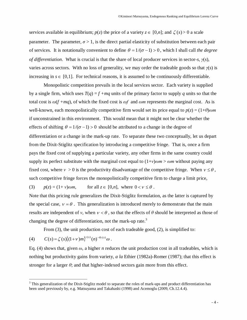
services available in equilibrium; p(z) the price of a variety z [0,n]; and )(s > 0 a scale

parameter. The parameter, σ > 1, is the direct partial elasticity of substitution between each pair

of services. It is notationally convenient to define 0)1/(1 , which I shall call the degree

of differentiation. What is crucial is that the share of local producer services in sector-s, γ(s),

varies across sectors. With no loss of generality, we may order the tradeable goods so that γ(s) is

increasing in s [0,1]. For technical reasons, it is assumed to be continuously differentiable.

Monopolistic competition prevails in the local services sector. Each variety is supplied

by a single firm, which uses T(q) = f +mq units of the primary factor to supply q units so that the

total cost is ω(f +mq), of which the fixed cost is ωf and ωm represents the marginal cost. As is

well-known, each monopolistically competitive firm would set its price equal to p(z) = (1+θ)ωm

if unconstrained in this environment. This would mean that it might not be clear whether the

effects of shifting 0)1/(1 should be attributed to a change in the degree of

differentiation or a change in the mark-up rate. To separate these two conceptually, let us depart

from the Dixit-Stiglitz specification by introducing a competitive fringe. That is, once a firm

pays the fixed cost of supplying a particular variety, any other firms in the same country could

supply its perfect substitute with the marginal cost equal to (1+ν)ωm > ωm without paying any

fixed cost, where ν > 0 is the productivity disadvantage of the competitive fringe. When ,

such competitive fringe forces the monopolistically competitive firm to charge a limit price,

(3) p(z) = (1+ ν)ωm, for all z [0,n], where 0 .

Note that this pricing rule generalizes the Dixit-Stiglitz formulation, as the latter is captured by

the special case, . This generalization is introduced merely to demonstrate that the main

results are independent of ν, when , so that the effects of θ should be interpreted as those of

changing the degree of differentiation, not the mark-up rate.3

From (3), the unit production cost of each tradeable good, (2), is simplified to:

(4) )()( )()1()()( ss nmssC .

Eq. (4) shows that, given ω, a higher n reduces the unit production cost in all tradeables, which is

nothing but productivity gains from variety, a la Ethier (1982a)-Romer (1987); that this effect is

stronger for a larger θ; and that higher-indexed sectors gain more from this effect.

3 This generalization of the Dixit-Stiglitz model to separate the roles of mark-ups and product differentiation has been used previously by, e.g. Matsuyama and Takahashi (1998) and Acemoglu (2009, Ch.12.4.4).


- 5 -

Since all the services are priced equally and enter symmetrically into production, q(z) = q

for all z [0,n], and the profit of all service providers is given by π(z) = pq − ω(mq + f) = ω(vmq

− f) for all z [0,n]. Thus, they earn zero profit if and only if:

(5) vmq = f,

which holds in equilibrium due to the free entry-and-exit to the service sector.

Before proceeding, note that we may set,

(6) B(s) = s for all s [0,1],

so that β(s) = 1 for all s [0,1] by choosing the tradeable goods indices, without further loss of

generality.4 In words, we measure the size of (a set of ) sectors by the expenditure share of the

goods produced in these sectors. With this indexing, the size of sectors whose γ is less than or

equal to γ(s) is equal to s, and a country’s share in the world income is equal to the measure of

the tradeables for which the country ends up having comparative advantage in equilibrium.

2.2 Single-Country (or Autarky) Equilibrium (J = 1)

First, let us look at the equilibrium allocation of a one-country world (J = 1). This can

also be viewed as the equilibrium allocation of a country in autarky in a world with multiple

countries, which would serve as the benchmark for evaluating the welfare effects of trade.

Because of Cobb-Douglas preferences, the economy must produce all the consumption

goods in the absence of trade, which means that their prices must be equal to their costs; that is,

(7) )()( )()1()()()( ss nmssCsP for all s [0,1]

Since the representative consumer spends β(s)Y = Y on good-s, and sector-s spends 100γ(s)% of

its revenue on producer services, the total revenue of the producer services sector is

(8) npq = n(1+ν)mωq = 1

0

)()( Ydsss = A Y, where 1

0

)( dssA .

Thus, in autarky, the share of the producer services in the aggregate income is equal to the

average share of the producer services across all the consumption goods sectors. Likewise,

sector-s spends 100(1−γ(s))% of its revenue on the primary factor. In addition, each service

provider spends ω(f+mq) on the primary factor. The total income earned by the (composite)

4 To see this, starting from any indexing of the goods s' [0,1] satisfying i) )'(~ s [0,1] is increasing in s' [0,1],

ii) )'(~ s > 0 for s' [0,1], and iii) 1')'(~1

0 dss , re-index the goods by

'

0)(~)'(~ sduusBs . Then,

))(~(~)( 1 sBs is increasing in s [0,1] and ')'(~ dssds , so that β(s) = 1 for s [0,1].


- 6 -

primary factor is thus equal to:

(9) ωV = 1

0

)())(1( Ydsss + nω(f+mq) = (1−Γ A)Y + nω(f+mq).

Combining (8) and (9) with the zero-profit condition (5) yields the equilibrium variety of

services (and the number of service providers) as well as the aggregate income:

(10)

f

Vn AA

1

(11) YA = ωAV = ωAF(K,L,…).

Eq. (10) shows that the equilibrium variety, nA, is proportional to the share of producer services

in the total expenditure, which is equal to A in autarky. Eq.(11) shows that, because free entry

ensures zero profit, the aggregate income is accrued entirely to the primary factors. With all the

primary factors, capital (K), labor (L), etc. being aggregated into the composite, V =F(K,L,…),

the equilibrium price of the composite factor, ωA, is nothing but TFP, as measured in GDP

accounting.

2.3 Stable Multi-Country Equilibrium (J ≥ 2)

Let us now turn to the case with J ≥ 2. Since these countries are ex-ante identical, they

share the same values for all the exogenous parameters. However, the stability of equilibrium

requires that no two countries share the same value of n, as explained later. This allows us to

rank the countries such that Jjjn

1is (strictly) increasing in j. (The subscript here indicates the

rank, not the identity, of a country in a particular equilibrium.) Then, from (4), the relative cost

between the j-th and the (j+1)-th countries,

1

)(

11 )()(

j

j

s

j

j

j

j

nn

sCsC

,

is increasing in s for any j = 1, 2, ..., J−1, for any combination of the factor prices Jjj 1

, as

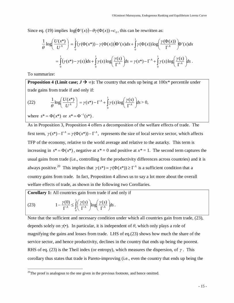
illustrated by upward-sloping curves in Figure 1. In words, a country with a more developed

local support industry has comparative advantage in higher-indexed sectors, which rely more

heavily on local services. Furthermore, Jjj 1

must adjust in equilibrium so that each country

becomes the lowest cost producer (and hence the exporter) of a positive measure of the tradeable


- 7 -

goods.5 This implies that a sequence, JjjS

0, defined by S0 = 0, SJ = 1, and

1)(

)(

1

)(

11

j

j

S

j

j

jj

jjj

nn

SCSC

(j = 1, 2, ..., J−1),

is increasing in j.6 As showed in Figure 1, the tradeable goods, [0,1], are partitioned into J

subintervals of positive measure, (Sj−1, Sj), such that the j-th country becomes the lowest cost

producer (and hence its sole producer and exporter) of s (Sj−1, Sj).7 Note also that the

definition of 1

1

JjjS can be rewritten to obtain:

(12) 1)(

11

jS

j

j

j

j

nn

. (j = 1, 2, ..., J−1)

so that Jjj 1

is also increasing in j; that is, a country with a more developed local support

industry (i.e., a higher j) is more productive due to the variety effect.

Since the j-th country specializes in (Sj−1, Sj), 100(Sj−Sj−1)% of the world income, YW, is

spent on its tradeable sectors, and its sector-s in (Sj−1, Sj) spends 100γ(s)% of its revenue on its

local services. Thus, the total revenues of its local producer services sector is equal to

(13) njpjqj = nj(1+ν)mωjqj =

j

j

S

S

dss1

)( YW = (Sj−Sj−1)ГjYW, (j = 1, 2, ...,J )

where

(14)

j

j

S

Sjjjjj dss

SSSS

1

)(1),(1

1 . (j = 1, 2, ...,J )

is the average of over (Sj−1, Sj). Note that Jjj 1

is increasing in j, since is increasing in s.

Likewise, in the j-th country, sector-s (Sj−1, Sj) spends 100(1−γ(s))% of its revenue on its

primary factor, and each service provider spends ωj(f+mqj) on its primary factor. Thus, the total

income earned by the primary factor in the j-th country is equal to:

(15) ωjV = (1− Гj)(Sj−Sj−1)YW + njωj(mqj + f) (j = 1, 2, ...,J ) 5 Otherwise, the factor price would be zero for a positive fraction (at least 1/J) of the world population. 6To see why, Sj ≥ Sj+1 would imply Cj (s) > min{Cj–1(s), Cj+1(s)} for all s [0,1], hence that the j-th country is not the lowest cost producers of any tradeable good, a contradiction. 7 In addition, S0 is produced and exported by the 1st country and SJ by the J-th country. The borderline sector, Sj (j = 1, 2,…, J−1), could be produced and exported by either j-th or (j+1)-th country or both. This type of indeterminacy is inconsequential and ignored in the following discussion.


- 8 -

Combining (13) and (15) with the zero-profit condition (5) yields:

(16)

f

Vn jj

1; (j = 1, 2, ...,J )

and

(17) Wjjjj YSSVY )( 1 . (j = 1, 2, ...,J )

Because Jjj 1

is increasing in j, eq.(16) shows that Jjjn

1is also increasing in j, as has been

assumed. Eq.(17) shows that j represents TFP of the j-th poorest country, and 1 jjj SSs ,

the size of the tradeable sectors in which this country has comparative advantage, is also equal to

its share in the world income. Thus,

j

k kj sS1

is the cumulative share of the j poorest

countries in world income. By combining (12), (14), (16), and (17), we obtain:

Proposition 1: Let jS be the cumulative share of the j poorest countries in world income.

Then, JjjS

0 solves the second-order difference equation with two terminal conditions:

(18) 1),(),(

)(

1

1

1

1

jS

jj

jj

jj

jj

SSSS

SSSS

with 00 S & 1JS , where 1

11

)(),(

jj

S

Sjj SS

dssSS

j

j

.

Figure 2 illustrates a solution to eq. (18) by means of the Lorenz curve, ]1,0[]1,0[: J ,

defined by the piece-wise linear function, with jJ SJj )/( . From the Lorenz curve, we can

recover Jjjs

0, the distribution of the country shares and vice versa.8 A few points deserve

emphasis. First, because ),( 1 jjj SS is increasing in j, jj ss /1 /)( 1 jj SS )( 1 jj SS >

1. Hence, the Lorenz curve is kinked at Jj / for each j = 1, 2, ..., J−1. In other words, the

ranking of the countries is strict.9 Second, since both income and TFP are proportional to

1 jjj SSs , the Lorenz curve here also represents the Lorenz curve for income and TFP.

Third, we could also obtain the ranking of countries in other variables of interest that are

8 This merely states that there is a one-to-one correspondence between the distribution of income shares and the Lorenz curve. With J ex-ante identical countries, there are J! (factorial) equilibria for each Lorenz curve. 9This is in sharp contrast to Matsuyama (1996), a closest precedent to the present paper, which shows a non-degenerate distribution of income across countries, but with a clustering of countries that share the same level of income. The crucial difference is that the countries outnumber the tradeable goods in the model of Matsuyama (1996), while it is assumed here, more realistically, that the tradabable goods outnumber the countries.


- 9 -

functions of Jjjs

0. For example, the j-th country’s share in world trade, is equal to

J

k kkjj ssss1

22 / , which is increasing in j . The j-th country’s trade dependence,

defined by the volume of trade divided by its GDP, is equal to js1 , which is decreasing in j.

2.4 Symmetry-Breaking: Instability of Equilibria without Strict Ranking of Countries

In characterizing the above equilibrium, we have started by imposing the condition that

no two countries share the same value of n, and hence the countries could be ranked strictly so

that Jjjn

1is increasing in j, and then verified later that this condition holds in equilibrium.

Indeed, there are also equilibria, in which some countries share the same value of n, and without

strict ranking, Jjjn

1is merely nondecreasing in j. For example, consider the case of J = 2 and

suppose n1 = n2 in equilibrium. Then, from (4), 2121 /)(/)( sCsC , which is independent of

s. Thus, the condition under which each country produces a positive measure of goods is

satisfied only if 2121 /)(/)( sCsC = 1. This means that, in this equilibrium, the consumers

everywhere is indifferent as to which country they purchase tradeable goods from. In other

words, the patterns of trade are indeterminate. If exactly 50% of the world income is spent on

each country’s tradeable goods sectors, and if this spending is distributed across the two

countries in such a way that the local services sector of each country ends up receiving exactly

2/A fraction of the world spending, then free entry to this sector in each country would lead to

n1 = n2 = nA. Thus, the two countries remain identical ex-post. However, it is easy to see that

this symmetric equilibrium, which replicates the autarky equilibrium in each country, is “sitting

on the knife-edge”, in that the required spending patterns described above must be met exactly in

spite of the consumers’ indifference. Furthermore, this symmetric equilibrium is unstable with

respect to best-response type dynamics. To see this, imagine that small random perturbations

make n1 slightly lower than n2. This would leads to a change in the spending patterns that makes

the profit of local service providers in country 1 lower than that in country 2, creating a force

towards a further decline in n1 and a further increase in n2 , pushing the world further away from

the symmetric allocation. This logic carries over to the case of J > 2 with nj = nj+1 for some j,

because that would imply 1/)(/)( 11 jjjj sCsC so that, for a positive measure of goods,

the consumers would be indifferent between buying from the j-th or (j+1)-th country, which


- 10 -

would generate the same knife-edge property. For this reason, we restrict ourselves only to the

equilibrium with a strict ranking of countries.10

The symmetry-breaking mechanism that renders equilibrium without strict ranking

unstable and leads to the emergence of strict ranking across ex-ante identical countries is a two-

way causality between the patterns of trade and cross-country productivity differences. A

country with a more developed local services sector not only has higher TFP, but also

comparative advantage in tradeable sectors that depend more on local services. Having

comparative advantage in such sectors means a larger local demand for such services, which

leads to a more developed local services sector and hence higher TFP. Since tradeable goods

differ in their dependence of local services, some countries end up becoming less productive and

poorer than others. Although many similar symmetry-breaking mechanisms exist in the trade

and geography literature, they are usually demonstrated in models with two countries/regions.

One advantage of the present model is that, with a continuum of goods, the logic extends to any

finite number of countries/regions.

2.5 Equilibrium Lorenz Curve: Limit Case (J ∞)

Even though eq. (18) fully characterizes the equilibrium distribution of country shares, it

is not analytically solvable. Of course, one could try to solve it numerically. However,

numerical methods are not useful for answering the question of the uniqueness of the solution or

for determining how the solution depends on the parameters of the model. Instead, in spirit

similar to the central limit theorem, let us approximate the equilibrium Lorenz curve with a large

but a finite number of countries by J

Jlim .11 It turns out that, as J ∞, eq.(18)

converges to the second-order differential equation with two terminal conditions, whose solution

is unique and can be solved analytically.12 This allows us to study not only what determines the

shape of the Lorenz curve, but also conduct various comparative statics, and to evaluate the

welfare effects of trade.

10 The logic behind the instability of equilibrium without strict ranking of countries is similar to that of the mixed strategy equilibrium in games of strategic complementarity, particularly the game of the battle of the sexes. The assumption of a finite number of countries is crucial. The assumption of zero trade cost in tradeable goods is not crucial but simplifies the argument significantly; See Matsuyama (2012; footnote 11) for more detail. 11 Note that this is different from assuming a continuum of countries, as eq.(18) is derived under the assumption that there are a finite number of countries. 12From this, the Lorenz curve is unique for a sufficiently large J. Whether the Lorenz curve is unique for any finite J is an open question. I conjecture that it is.


- 11 -

Here’s how to obtain the limit Lorenz curve, J

Jlim . The basic strategy is to

take Taylor expansions on both sides of eq. (18).13 First, by setting Jjx / and Jx /1 ,

221

2

)(")(')()( xoxxxxxxSS xjj

,

221

2

)(")(')()( xoxxxxxxSS xjj ,

from which the LHS of eq. (18) can be written as:

xoxxx

SSSS

jj

jj

)(')("1

1

1 .

Likewise,

)()('))(('21))((

)()(

)(),(

)(

)(1 xoxxxx

xxx

dssSS

xx

xjj

)()('))(('21))((

)()(

)(),(

)(

)(1 xoxxxx

xxx

dssSS

x

xxjj

from which the RHS of eq.(18) can be written as:

))(()(

1

1 )('))(())(('1

),(),( xS

jj

jj xoxxxx

SSSS j

xoxxx )('))(('1 .

By combining these, eq.(18) becomes:

xoxxxxoxxx

)('))(('1)(')("1 .

By letting 0/1 Jx , this becomes:

(19) )('))((')(')(" xx

xx

.

Integrating (19) twice yields xecdse cx s 01

)(

0

)( xdue u

1

0

)( , where two integral

constants, c0 and c1, are pinned down by the two terminal conditions, 0)0( and 1)1( .

This can be further rewritten as follows:

Proposition 2: The limit equilibrium Lorenz curve, JJ lim = , is given by:

13 Initially, I obtained the limit by a different method, which involves repeated use of the mean value theorem. I am grateful to Hiroshi Matano for showing me this (more efficient) method, without which I might not have been able to study two extensions in section 3.


- 12 -

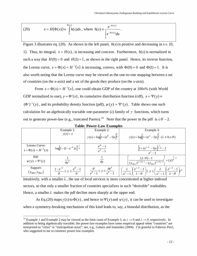
(20)

)(

0

)()(x

dsshxHx , where

1

0

)(

)(

)(due

eshu

s

.

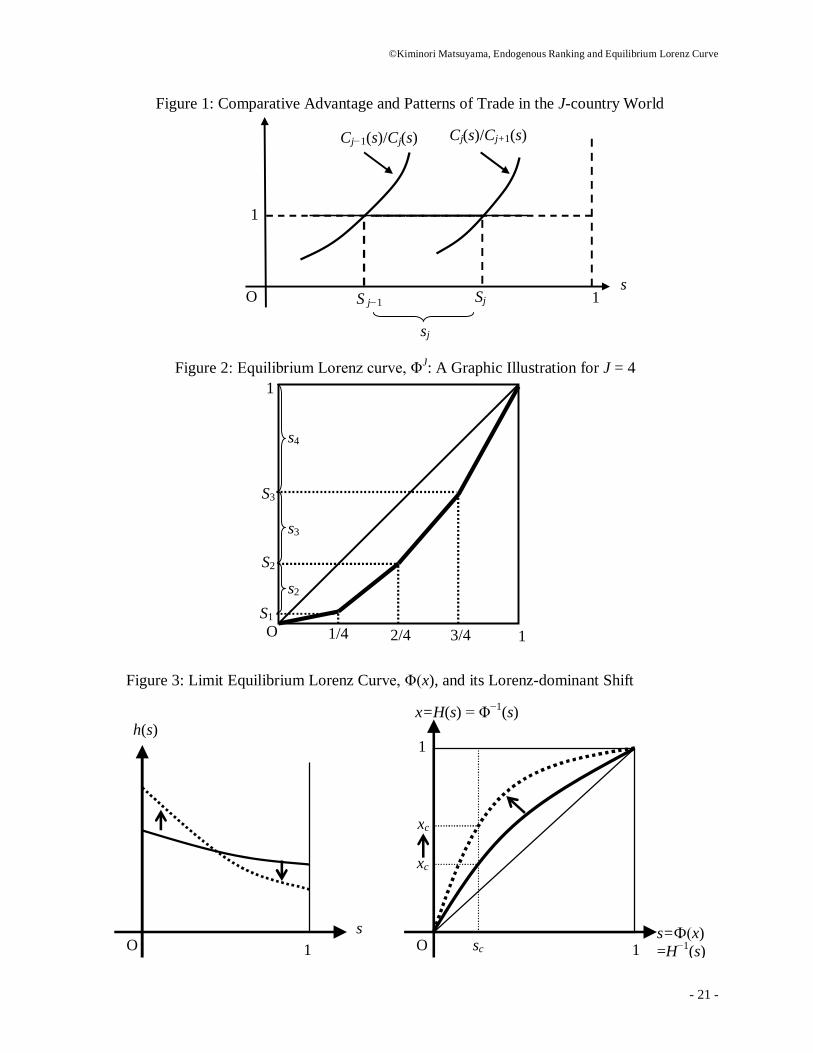
Figure 3 illustrates eq. (20). As shown in the left panel, )(sh is positive and decreasing in s [0,

1]. Thus, its integral, )(sHx , is increasing and concave. Furthermore, )(sh is normalized in

such a way that 0)0( H and 1)1( H , as shown in the right panel. Hence, its inverse function,

the Lorenz curve, xHxs 1)( is increasing, convex, with 0)0( and 1)1( . It is

also worth noting that the Lorenz curve may be viewed as the one-to-one mapping between a set

of countries (on the x-axis) and a set of the goods they produce (on the s-axis).

From xHxs 1)( , one could obtain GDP of the country at 100x% (with World

GDP normalized to one), )(' xy , its cumulative distribution function (cdf), )( yx

)()'( 1 y , and its probability density function (pdf), )(y )(' y . Table shows one such

calculation for an algebraically tractable one-parameter (λ) family of functions, which turns

out to generate power-law (e.g., truncated Pareto).14 Note that the power in the pdf is λ/θ 2.

Table: Power-Law Examples Example 1:

ss )( Example 2:

1

)1(1log)( ses

Example 3:

1

)1(1log)( ses );0(

Lorenz Curve: )(xs )(1 xH

1

)1(1log xe 11

ee x

1

1)1(1

exe

Pdf: )(y )(' y 2

1y

y1

1)/(1)/( )()(1)/(

MinMax yy2

)(

y

Support: ],[ MaxMin yy ye

1

1

e 11

e

eye

yee

11

ee

e

11

Intuitively, with a smaller , the use of local services is more concentrated at higher-indexed

sectors, so that only a smaller fraction of countries specializes in such “desirable” tradeables.

Hence, a smaller makes the pdf decline more sharply at the upper end.

As Eq.(20) maps )(s to )(x , and hence to )(y and )(y , it can be used to investigate

when a symmetry-breaking mechanism of this kind leads to, say, a bimodal distribution, as the

14 Example 1 and Example 2 may be viewed as the limit cases of Example 3, as λ → 0 and λ → θ, respectively. In addition to being algebraically tractable, the power-law examples have some empirical appeal when “countries” are interpreted as “cities” or “metropolitan areas”: see, e.g., Gabaix and Ioannides (2004). I’m grateful to Fabrizio Perri, who suggested to me to construct power-law examples.


- 13 -

narrative in much of this literature, (“core-periphery” or “polarization”) seems to suggest. When

the (increasing and continuously differentiable function) can be approximated by a two-step

function, the corresponding pdf becomes bimodal. Thus, the world becomes polarized into the

rich core and the poor periphery, when the tradeable goods can be classified into two categories

in such a way that they are roughly homogeneous within each category.15 Generally, a

symmetry-breaking mechanism of this kind leads to N “clusters” of countries if can be

approximated by an N-step function.16

Another advantage of Eq.(20) is that one could easily see the effect of changing θ, as

illustrated by the arrows in Figure 3. To see this, note first that )()(ˆ sesh , the numerator of

)(sh , satisfies 0)('/))(ˆlog(2 sssh . In words, it is log-submodular in θ and s.17

Thus, a higher θ shifts the graph of )()(ˆ sesh down everywhere but proportionately more at a

higher s. Since )(sh is a rescaled version of )(ˆ sh to keep the area under the graph unchanged,

the graph of )(sh is rotated “clockwise” by a higher θ, as shown in the left panel. This “single-

crossing” in )(sh implies that a higher θ makes the Lorenz curve more “curved” and move

further away from the diagonal line, as shown in the right panel. In other words, a higher θ

causes a Lorenz-dominant shift of the Lorenz curve. Thus, any Lorenz-consistent inequality

measure, such as the generalized Kuznets Ratio, the Gini index, the coefficients of variations,

etc. all agree that a higher θ leads to greater inequality.18

2.6 Welfare Effects of Trade

The mere fact that trade creates ranking of countries, making some countries poorer than

others, does not necessarily imply that trade make them poorer. We need to compare the utility

15Formally, consider a sequence of (increasing and continuously differentiable) functions that converges point-wise to a two-step function, Ls )( for s ),0[ s and LHs )( for s ]1,(s . Then, the sequence of the

corresponding cdf’s converges to the cdf, )(y = 0 for )1)(1(1 esy ; )(y = 1])1/1(1[ es for

)1(1)1)(1(1 esyes , and )(y = 1 for )1(1 esy , where 0 LH . 16 Note that this is different from assuming that is a N-step function, which is equivalent to assume that there are N (a finite number of) tradeable goods. Then, the equilibrium distribution would not be unique; see Matsuyama (1996) for N = 2. To obtain the uniqueness, it is essential that is increasing, which means that the set of the tradeable goods is a continuum, and hence outnumbers the set of the countries for a large but finite number, J. 17See Topkis (1998) for mathematics of super-(and sub-)modularity and Costinot (2009) for a recent application to international trade. 18Likewise, any shift in γ(s) that rotates h(s) clockwise leads to greater inequality.


- 14 -

levels under trade and under autarky. From eq.(1), the welfare under autarky is

1

0)(logloglog dssPVU AAA . Likewise, the welfare of the country that ends up being

the j-th poorest can be written as 1

0)(logloglog dssPVU jj , where the tradeable goods

prices satisfy )()(

)()( s

Ak

Ak

s

Ak

Ak

A nn

sPsP

for s (Sk−1, Sk) for k = 1, 2, …, J.

Combining these equations yields

dssP

sPUU

AAj

Aj

1

0 )()(logloglog

J

k

S

SAk

S

SAk

Aj

k

k

k

k

dssds1 11

log)(loglog

,

which can be further rewritten as follows:

Proposition 3 (J-country case): The country that ends up being the j-th poorest under trade

gains from trade if and only if:

(21)

Aj

UU

log =

J

k

SSkj

kk

1

1/log

J

kkkA

kk SS

11)(log > 0.

Eq. (21) in Proposition 3 offers a decomposition of the welfare effects of trade. The first term is

the country’s TFP relative to the world average, and it is increasing in j , negative at j = 1 and

positive at j = J. The second term captures the usual gains from trade (i.e., after controlling for

the income and TFP differences across countries) and it is always positive. 19 However, aside

from rather obvious statements like “a country gains from trade if the second term dominates the

first term,” or “a country gains from trade if its income (and TFP) ends up being higher than the

world average,” Proposition 3 offers little insight without an explicit solution for eq. (18).

As J , the task of evaluating the overall welfare effect becomes greatly simplified.

By setting x* = j/J and x = k/J in eq. (21) and noting that )('/*)('/ xxkj and

dxxSS kk )('1 as J , eq.(21) converges to:

AUxU *)(log

1

0

1

0

)('))((log))(()(')('

*)('log dxxxxdxxxx

A

.

19Proof: Consider the convex maximization problem:

J

k kkkkc

SScMaxJkk

1 1)(log1

s.t. 1)(1 1

J

k kkk SSc .

Though 1kc satisfies the constraint, its optimum is reached at Akkc / , so that

J

k kkA

kk SS1 1)(/log

> 0)(1log1 1

J

k kkk SS .


- 15 -

Since eq. (19) implies 0))(()('log cxx , this can be rewritten as:

AUxU *)(log1

1

0

1

0

)('))((log))(()('))((*))(( dxxxxdxxxx A

1

0

1

0

)(log)()(*)( dsssdsss A

1

0

)(log)(*)( dssss AA .

To summarize:

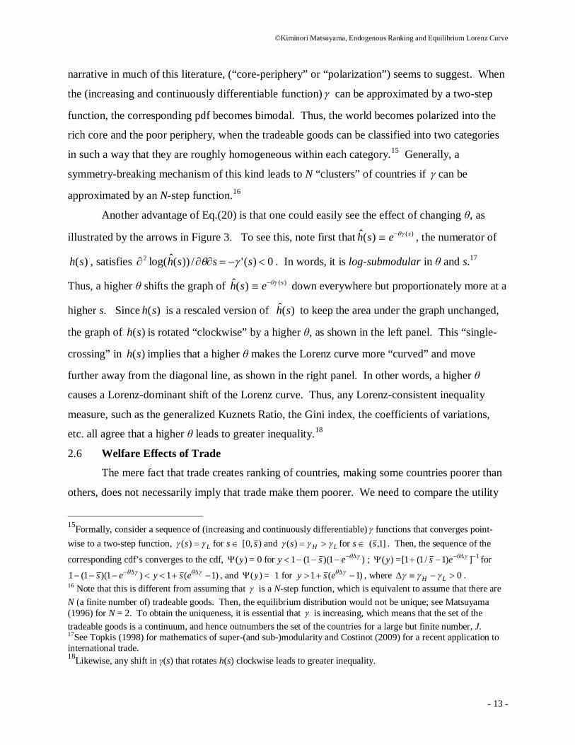
Proposition 4 (Limit case; J ∞): The country that ends up being at 100x* percentile under

trade gains from trade if and only if:

(22)

AUxU *)(log1

1

0

)(log)(*)( dssss AA > 0,

where *)(* xs or *)(* 1 sx .

As in Proposition 3, Proposition 4 offers a decomposition of the welfare effects of trade. The

first term, AA xs *))((*)( , represents the size of local service sector, which affects

TFP of the economy, relative to the world average and relative to the autarky. This term is

increasing in *)(* xs , negative at x* = 0 and positive at x* = 1. The second term captures the

usual gains from trade (i.e., controlling for the productivity differences across countries) and it is

always positive.20 This implies that Axs *))((*)( is a sufficient condition that a

country gains from trade. In fact, Proposition 4 allows us to say a lot more about the overall

welfare effects of trade, as shown in the following two Corollaries.

Corollary 1: All countries gain from trade if and only if

(23)

1

0

)(log)()0(1 dsssAAA

.

Note that the sufficient and necessary condition under which all countries gain from trade, (23),

depends solely on γ(•). In particular, it is independent of θ, which only plays a role of

magnifying the gains and losses from trade. LHS of eq.(23) shows how much the share of the

service sector, and hence productivity, declines in the country that ends up being the poorest.

RHS of eq. (23) is the Theil index (or entropy), which measures the dispersion, of . This

corollary thus states that trade is Pareto-improving (i.e., even the country that ends up being the

20The proof is analogous to the one given in the previous footnote, and hence omitted.


- 16 -

poorest would benefit from trade) when the tradeable goods are sufficiently diverse, as measured

by the Theil index of , and hence the gains from specialization (by making countries ex-post

heterogeneous) is sufficiently large.

Corollary 2: Suppose that (23) fails. Then, for cs > 0, defined by

)( cs

1

0

)(log)(1 dsssAA

A ,

a): All countries producing and exporting goods s [0, sc) lose from trade, while all countries

producing and exporting goods s (sc, 1] gain from trade.

b): The fraction of the countries that lose from trade, );( cc sHx , is increasing in θ , and

satisfies cc sx 0

lim

and 1lim cx

.

Corollary 2 is illustrated in the right panel of Figure 3. All countries that end up specializing in

[0, sc) lose from trade and they account for cx fraction of the world. Note that cs depends solely

on γ(•) and is independent of θ. This means that, as θ goes up and the Lorenz curve shifts, sc

remains unchanged and cx goes up. As varying θ from 0 to ∞ (i.e., σ from ∞ to 1), cx increases

from cs to 1. Thus, when γ is such that some countries lose from trade, virtually all countries

would lose from trade as the Dixit-Stiglitz composite approaches Cobb-Douglas.

3. Two Extensions

This section reports two extensions conducted in Matsuyama (2011, Section 3).

3.1 Nontradeable Consumption Goods: Globalization through Trade in Goods

The first extension allows a fraction of the consumption goods within each sector to be

nontradeable. This extension is used to examine the effects of globalization through trade in

goods. Suppose that each sector-s produces many varieties, a fraction τ of which is tradeable and

a fraction 1−τ is nontradeable, and that they are aggregated by Cobb-Douglas preferences.21 The

21 This specification assumes that the share of local differentiated producer services in sector-s is γ(s) for both nontradeables and tradeables. This assumption is made because, when examining the effect of globalization by changing τ, we do not want the distribution of γ across all tradeable consumption goods to change. However, for some other purposes, it would be useful to consider the case where the distribution of γ among nontradeable consumption goods differs systematically from those among tradeable consumption goods. For example, Matsuyama (1996) allows for such possibility to generate a positive correlation between per capita income and the nontradeable consumption goods prices across countries, similar to the Balassa-Samuelson effect.


- 17 -

expenditure function is now obtained by replacing ))(log( sP with ))(log()1())(log( sPsP NT

for each s [0,1], where ))}({)( sCMinsP jT is the price of each tradeable good in sector-s,

common across all countries, )()( sCsP jN is the price of each nontradeable good in sector-s,

which is equal to the unit of cost of production in each country. Following the steps similar in

section 2.3 and section 2.5, one could show:

Proposition 5: The limit Lorenz curve for GDP and TFP, JJ lim = , is given by

)(

0

);();(x

dsgshgxHx , where

1

0

)(/

)(/

/)(1

/)(1);(

dueug

esggsh

ugA

sgA

A

A

;

1

g > 0.

Again, Figure 3 illustrates the solution. For each )1/( g > 0, the left panel shows );( gsh

and the right panel );( gsH . It is also easy to verify );(lim0

gsh

= );(lim0

gshg

= 1. Thus, as τ 0,

each country converges to the same single-country (autarky) equilibrium and hence the Lorenz

curve converges to the diagonal line, and inequality disappears. Likewise, );(lim gshg

= )(sh

1

0

)()( / duee us . Thus, as τ 1, it converges to the one given in Proposition 2.

Indeed, a higher τ, as well as a higher θ, causes a Lorenz-dominant shift, as illustrated by

the arrows in Figure 3. To see this, one just need to check that the numerator of );( gsh ,

)(/

/)(1);(ˆ sgA esggshA

, is log-submodular in g and s (and in θ and s). This means

that both a higher τ and a higher θ make the graph of );( gsh rotate “clockwise,” and hence the

Lorenz curve becomes more “curved” and moves away from the diagonal line. This result thus

suggests that globalization through trade in goods leads to greater inequality across countries.

3.2 Variable Factor Supply: Effects of Factor Mobility and/or Factor Accumulation

The second extension allows variable supply in one of the components in the composite

of primary factors. This extension not only generates the correlation between the capital-labor

ratio and income and productivity, but also allows us to examine the effects of technical change

that increases importance of human capital or of globalization through factor mobility.


- 18 -

Returning to the case where τ = 1, let us now allow the available amount of the

composite primary factors, V, to vary across countries by endogenizing the supply of one of the

component factors, K, as follows:

(24) Vj = F(Kj,L) with ωjFK(Kj, L) = ρ.

where FK(Kj, L) is the first derivative of F with respect to K, satisfying FKK < 0. In words, the

supply of K in the j-th country responds to its TFP, ωj, such that its factor price is equalized

across countries at a common value, ρ. This can be justified in two different ways.

A. Factor Mobility: Imagine that L represents (a composite of) factors that are immobile across

borders and K represents (a composite of) factors that are freely mobile across borders, which

seek higher return until its return is equalized in equilibrium.22 According to this interpretation,

ρ is an equilibrium rate of return determined endogenously, although it is not necessary to solve

for it in order to derive the Lorenz curve.23

B. Factor Accumulation: Reinterpret the structure of the economy as follows. Time is

continuous. All the tradeable goods, s [0,1], are intermediate inputs that goes into the

production of a single final good, Yt, as

1

0))(log(exp dssXY tt so that its unit cost is

1

0))(log(exp dssPt . The representative agent in each country consumes and invests the final

good to accumulate Kt, so as to maximize

0)( dteCu t

t s.t.

ttt KCY , where ρ is the

subjective discount rate common across countries. Then, the steady state rate of return on K is

equalized at ρ. 24 With this interpretation, K may include not only physical capital but also

human capital, and the Lorenz curve below represents steady state inequality across countries.

With this modification and with V = F(K, L) = AKαL1−α, with 0 < < /11 =

22Which factors should be viewed as mobile or not depends on the context. If “countries” are interpreted as smaller geographical units such as “metropolitan areas,” K may include not only capital but also labor, with L representing “land.” Although labor is commonly treated as immobile in the trade literature, we will later consider the effects of globalization via factor mobility, in which case certain types of labor should be included among mobile factors. 23Also, Yj = Vj = ωjF(Kj, L) should be now interpreted as GDP of the economy, not GNP, and Kj is the amount of K used in the j-th country, not the amount of K owned by the representative agent in the j-th country. This also means that the LHS of the budget constraint in the j-th country should be its GNP, not its GDP (Yj). However, calculating the distributions of GDP (Yj), TFP (ωj), and Kj/L does not require to use the budget constraint for each country, given that all consumption goods are tradeable (τ = 1). The analysis would be more involved if τ < 1. 24The intertemporal resource constraint assumes not only that K is immobile but also that international lending and borrowing is not possible. Of course, these restrictions are not binding in steady state, because the rate of return is equalized across countries at ρ.


- 19 -

)1/(1 , Matsuyama (2011, Section 3.2) shows:

Proposition 6: The limit Lorenz curve for Y/L (and K/L), JJ lim = , is given by:

)(

0

);();(x

dsshxHx , where

1

0

/1

/1

)(1

1

)(1

1);(

duu

ssh

.

Again, Figure 3 illustrates the limit Lorenz curve for Y/L (and K/L), .25 For each < /11

= )1/(1 , the left panel shows );( sh and the right panel );( sH . Since );(lim0

sh

= )(sh

1

0

)()( / duee us , the solution converges to the one in Proposition 2, as α 0.

Indeed, a higher α, as well as a higher θ, causes a Lorenz-dominant shift, as illustrated by

the arrows in Figure 3. The reasoning should be familiar by now. The numerator of );( sh ,

/1)()]1/([1);(ˆ ssh , is log-submodular in α and s (and in θ and s). Thus, a higher α

(and a higher θ) makes the graph of );( sh rotate “clockwise,” and hence a Lorenz-dominant

shift, as shown in the right panel. This result suggests that skill-biased technological change that

increases the share of human capital and reduces the share of raw labor in production, or

globalization through trade in some factors, both of which can be interpreted as an increase in α,

could lead to greater inequality across countries.

References:

Acemoglu, D., Introduction to Modern Economic Growth, Princeton University Press, 2008. Combes, P.-P., T. Mayer and J. Thisse, Economic Geography, Princeton University Press, 2008. Costinot, A., “An Elementary Theory of Comparative Advantage,”Econometrica, 2009, 1165-92. Dixit, A. K., and J. E. Stiglitz, “Monopolistic Competition and Optimum Product Diversity,”

American Economic Review, 1977, 297-308. Dornbusch, R., S. Fischer, and P. A. Samuelson, “Comparative Advantage, Trade, and Payments

in a Ricardian Model with a Continuum of Goods,” American Economic Review, 67 (1977), 823-839.

Ethier, W., “National and International Returns to Scale in the Modern Theory of International Trade,” American Economic Review, 72, 1982, 389-405. a)

Ethier, W., “Decreasing Costs in International Trade and Frank Graham’s Argument for Protection,” Econometrica, 50, 1982, 1243-1268. b)

25 The limit Lorenz curve for TFP(ω) can be obtained from , by )(x

1

0

1

0

1 )('/)(' duuduux

.


- 20 -

Fujita, M., P., Krugman, P. and A. Venables, The Spatial Economy, MIT Press, 1999. Gabaix, X., and Y.M. Ioannides, “The Evolution of City Size Distributions,” in J.V. Henderson

and J.F. Thisse (eds.) Handbook of Regional and Urban Economics, Elsevier, 2004. Helpman, E., “Increasing Returns, Imperfect Markets and Trade Theory,” Chapter 7 in

Handbook of International Economics, edited by R. Jones and P. Kenen, 1986. Ioannides, Y., “Emergence,” in L. Blume and S. Durlauf, eds., New Palgrave Dictionary of

Economics, 2nd Edition, Palgrave Macmillan, 2008. Krugman, P. and A. Venables, “Globalization and Inequality of Nations,” Quarterly Journal of

Economics, 110 (1995), 857–80. Lewis, W.A. The Evolution of the International Economic Order,Princeton University Press, 1977. Matsuyama, K., “Why Are There Rich and Poor Countries?: Symmetry-Breaking in the World

Economy,” Journal of the Japanese and International Economies, 10 (1996), 419-439. Matsuyama, K., “Symmetry-Breaking” in L. Blume and S. Durlauf, eds., New Palgrave

Dictionary of Economics, 2nd Edition, Palgrave Macmillan, 2008. Matsuyama, K., “Endogenous Ranking and Equilibrium Lorenz Curve Among (ex-ante)

Identical Countries,” May 2011 version, http://faculty.wcas.northwestern.edu/~kmatsu/. Matsuyama, K., “Endogenous Ranking and Equilibrium Lorenz Curve Among (ex-ante)

Identical Countries,” Nov 2012 version, http://faculty.wcas.northwestern.edu/~kmatsu/. Matsuyama, K., and T. Takahashi, “Self-Defeating Regional Concentration,” Review of

Economic Studies, 65 (April 1998): 211-234. Myrdal, G. Economic Theory and Underdeveloped Regions, Duckworth, 1957. Romer, P., “Growth Based on Increasing Returns Due to Specialization,” American Economic

Review, 77 (1987), 56-62. Topkis, D., Supermodularity and Complementarity, Princeton University Press, 1998.


- 21 -

O 1

s

h(s)

O 1

s=Ф(x) =H−1(s)

1

x=H(s) = Φ−1(s)

Figure 3: Limit Equilibrium Lorenz Curve, Φ(x), and its Lorenz-dominant Shift

sc

xc

xc

S j−1 s

1

Cj−1(s)/Cj(s) Cj(s)/Cj+1(s)

Sj

sj

1 O

Figure 1: Comparative Advantage and Patterns of Trade in the J-country World

2/4 O

1

1 3/4 1/4

S3

S2

S1

s4

s3

s2

Figure 2: Equilibrium Lorenz curve, ΦJ: A Graphic Illustration for J = 4

Endogenous Ranking and Equilibrium Lorenz …faculty.wcas.northwestern.edu/~kmatsu/Endogenous...

Documents

Transcript of Endogenous Ranking and Equilibrium Lorenz …faculty.wcas.northwestern.edu/~kmatsu/Endogenous...