THE DEMAND FOR EDUCATION IN PUBLIC AND PRIVATE …

Journal of Public Economics 3 (1974) 349-385. 0 North-Holland Publishing Company

THE DEMAND FOR EDUCATION IN PUBLIC AND PRIVATE SCHOOL SYSTEMS*

J. E. STIGLITZ

Stanford University, Stanford, Cali/. 94305, U.S.A.

1. Introduction

This paper is concerned with the demand for education under various institutional arrangements. Education has a number of properties which make the analysis of the demand for it both interesting and complex.

First, education is provided in the United States both publicly and privately; although there are a few other publicly provided goods which are also privately supplied (e.g., police protection), education is perhaps the most important public good in which both public and private provision plays an important role.

Secondly, primary responsibility for education in the United States has traditionally been placed on local governmental bodies, and hence the analysis of the demand and supply of education involves an analysis of local public goods and the relations between local and other governmental bodies.

Thirdly, education is itself a complex commodity. It is a consumption good and a capital good, i.e., although much of the expenditure is justified in terms of the effects on the individual’s income in the future, many of the activities of educational institutions are primarily justifiable in terms of their immediate consumption benefits. Moreover, education affects individuals’ future incomes both by providing skills and by providing inforniation about individuals’ characteristics (the human capital versus the screening views of education). It is both a public good and a private good; that is, most of the benefits of education accrue directly to those who are being educated, although public education has been defended on the social return to having an educated citizenry. (Presumably; this refers to social returns which are not captured by the individual himself. I am a little skeptical about the importance of the social returns which are in excess of the private returns.) Finally, public education has traditionally been defended for its redistributive effects, i.e., for providing a good (which may in fact be a private good) to children independently of the wealth of the parents of the children, yet more recently it has been attacked as major contributor to inequality.

*Paper presented to the September 1973 Siena meeting of the International Seminar on Public Economics. The author is indebted to A.B. Atkinson for helpful comments. Research support of the National Science Foundation is gratefully acknowledged.

D

350 J. E. Stiglitz, Demand for education

What I propose to do here, rather than to treat education in all of its com- plexity, is to consider the demand for education in each of its separate roles.

The basic burden of this paper is to suggest that the equilibrium level of expenditure on education is likely to differ markedly depending on the institutional arrangement for its provision - public, mixed private-public, or purely private - but in none of these cases is the level of expenditure necessarily Pareto Optimal. In some cases, there is a clear presumption that public provision leads to an under-supply, while in other cases, there is some presumption that there will be an oversupply.

Sections 2-4 treat education in its conventional aspects as a consumption good and as providing ‘human capital’, while section 5 investigates the role of education in providing information about individuals’ characteristics. Regret- ably, the analysis quickly becomes very complex. Thus the analysis is developed in detail only for some special cases, but it is hoped that the insights gained are of more general applicability.

2. Pure public goods and pure publicly provided private goods

A pure public good is conventionally defined as a good which has two characteristics: (a) the marginal cost of an additional person consuming it is zero; (b) the cost of excluding an individual from its benefits is infinite (pro- hibitive).

A pure publicly provided private good is a private good (a good for which there is a substantial marginal cost of an additional person consuming it) which is provided in equal quantities to all individuals (within a given class) without charge. There may be several reasons for providing such goods publicly; there may be high costs of exclusion (high costs of charging for the particular services performed) or there may be ethical (distributional) grounds for providing it publicly. (All individuals ‘ought’ to receive equal medical treatment independently of their ability to pay; the education of children ‘ought not’ to depend on the wealth of their parents.)

In most developed economies, education is publicly provided; and there seems little question that the marginal cost of educatin, w an additional individual is

substantial (probably close to the average cost, at least for large school systems). Yet there remains some dispute about whether it is best thought of as a pure public good or as a pure publicly provided private good. The dispute can be thought of in the following way. Let %lI be the individual’s utility function, and among its potential arguments are the levels of education, Ei, of each individual in society, including himself,

~’ = -ly-‘(E,, E,,... Ej,...E”,...). (9

Clearly, if education were a pure private good, then we could write

-W’ = ~‘(Ej,...), (1’)

J. E. Stiglitz, Demand for education 351

not depending on Ei, i # j. On the other hand, if the sole benefit of education were an educated citizenry, which affected the ‘quality of government’ then we could write the utility function in the following form,’

W-j = W’($(E,, . . . . E,), . ..). all j. (1”)

A special case of (1”) is the conventional formulation for a pure public good,

9-j = w-j (iglE,,...).

There are obviously ‘mixed’ cases where the ith individual’s consumption of education enters the jth individual’s welfare but not ‘symmetrically’, and education is clearly one of those ‘mixed cases’. Such a case we might depict by2

Yfj = Wi(Ej, $(E, , . . ., E,), . . .).

Analytically, we need to make two distinctions:

( 1”‘)

(a) Even if at low levels of El, . . . E,, there may be public goods aspects of education, these may reach saturation at levels of expenditure on education below those which would be privately demanded. That is, if Ef is the equilibrium level of consumption of education by the ith individual in a purely private school system, then

W:(EP, 4(E:, . . . , E,p), . ..) = 0, all j. (2)

In such a case, although there are public goods aspects of education, for resource allocation purposes, these public goods aspects may be ignored. Those who say that education is ‘basically’ a private good are, I think, saying that it is not unrealistic to assume that condition (2) holds.

(b) Although pure publicly provided private goods and pure public goods represent very diflerent kinds of commodities, the conditions for Pareto Optimality (appropriately interpreted) are identical: the sum of the marginal rate of substitution must equal the marginal rate of transformation, where the marginal cost of providing one elitra unit of the ‘pure publicly pro&ded private good’ is interpreted to mean providing one extra unit of the good to everyone.

To see this, assume for simplicity that there is a single privately provided private good, P, so the jth individual’s welfare may be written as

Wj = W-‘(Ej, Pi), (3)

IIt should be noted that in this representation, we are in effect considering education as an intermediate good.

2There are obviously other representations of mixed cases. In some sense, any representation of the form YF’-J(E, ,. . . , En, . ..). in which WrJ # 0 and which cannot be written in the form (l”), can be considered to be a ‘mixed’ case.

352 J. E. Sliglitz, Demand for education

and that there is a production possibilities schedule for the economy of the form

T(x Ej, cPj) = 0. (4)

We assume there are N individuals, so for a pure publicly provided private good, cj Ej = NE. Then Pareto Optimality requires maximization of, say W’, given W2,..., W”, subject to the constraint (4). Forming the Lagrangian

9 = CA’w’(E, Pj) + pT(NE, 1 Pj) >

we obtain first-order conditions,

which may be rewritten

aYfi/i3Ej NT,

mPj=Tp’ (5)

the required result. In the next section, we analyze the relationship between the equilibrium supply

of education and the Pareto Optimal level. It makes no difference for our analysis whether education is considered to be a pure public good or a pure publicly provided private good, so long as all individuals go to public schools. What does make a difference is that under certain circumstances, if education is a private good, it may pay for some individuals to purchase (in addition to or in place of public education) some private education. This seriously complicates the analysis of the demand for education, and is considered separately in the subsequent section.

3. Comparison between majority voting equilibrium and Pareto Optimality

The object of this section is to consider the relationship between the allocation to public goods (whether pure public goods or publicly provided private goods) which emerges in a majority voting democracy with the Pareto Optimal allocation. The results reported in section 3.1 apply to any public good; these results are applied to education in section 3.2.

The question of whether there is a systematic bias in providing too little or too much public goods is a subject which has been extensively debated by political economists and journalists : one hears simultaneously complaints about the starvation of public services amidst private affluence and complaints about excessively high tax rates and excessive government expansion. The explanation of w.hy there is too ‘much’ or too little public expenditure is often associated with judgments concerning the nature of the political process. Those who see there being too little expenditure often argue that the political process under-represents the poor; those who see there being too much expenditure argue that, in


democratic systems, since the poor have an equal vote with the rich, but bear a relatively small proportion of the costs of government expenditure, there is a natural tendency for democratic systems to have excessive expenditures. Neither side usually makes clear the welfare norm against which such statements are being made.

In the discussion below, we will not directly address ourselves to the political judgments implicit in much of this debate. Rather, we shall simply examine the outcome of a majority voting process. Intuitively, neither side in the above argument is convincing: if the good that is being provided is a public good, the fact that the poor do not contribute to the cost of its provision yet benefit from it does not subtract from the benefits which accrue to the rich. The vested interests of the rich in the provision of some public goods, like police protection and perhaps education, would seem to be at least as great as that of the poor. On the other hand, although the poor do contribute less to the provision of the public good, their marginal utility of private goods is also higher than that of

the rich, and so long as they contribute something, the poor may actually be relatively ‘low demanders’. The answer provided in the analysis of section 3.1 is, not surprisingly, that ‘it depends’; under our simplifying assumptions, however, we are able to show that it depends on just two parameters.

There is a second, quite different, strand of literature which has been concerned with the allocation of resources to public goods. This has been concerned with the problems of getting individuals to reveal their true preferences. On the one hand, if the amount a particular individual has to pay depends on this revealed demand for thi public good, there will be a tendency to under-represent one’s true preferences; on the other hand, some of the recent literature on the revelation of demands has been based on the hypothesis of lump sum taxation, so that the level of demand of the public good revealed by the individual does not directly affect the taxes the individual pays. It has been argued that in this case, individuals will reveal their true preferences.

In most economies, however, there is a close link between the level of expenditure and the level of taxation which an individual has to pay, but not a direct link between a particular individual’s revealed demand and the amount he has to pay. This means’ that the demands ex’pressed by individuals in the political process depend on the particular tax system employed; but it also means that rhe demands expressed will not be the demands they would have expressed were there lump sum taxation, but neither are they the ‘zero demands’ they would have expressed if their taxes depended on the particular level of demand for public gocds which they expressed.

Again, it is not obvious without a closer examination whether, given simple tax structures, the equilibrium level of public expenditure will be too small or too large (greater or less than the Pareto Optimal level).

For local public goods, taxes are simply proportional to expenditure, and this is the hypothesis which we shall adopt throughout this paper.


3.1. The zenera case

The model we present in this section is consistent with education being either a consumption or an investment good, a pure public good or a pure publicly provided private good.

We let G be the level of expenditure on the public good. We assume that the set of voters and of taxpayers are identical. Wealth (assumed to be given exo- genously) of the ith individual is denoted by Wi. Thus total national wealth is just

1 Wi = IF’N, (6)

where N is the number of voters in the economy, and IV is mean wealth. Thus if public expenditures are financed by proportional income taxes, and if z is the tax rate, then

G = rrN. (7)

The ith individual votes for the level of public expenditure which maximizes his utility. We represent utility as a function of the expenditure on the public good (G) and on the private good, P. P is just his after tax wealth,

Pi = (I-Z)Wi. (8)

Thus he maximizes

(9) is maximized when

(10)

i.e., when the individual’s marginal rate of substitution between public and private goods is equal to the ratio of his wealth to total wealth. In particular, if YV is quasi-concave, then preferences are single-peaked, and the majority voting equilibrium will be the level of demand of the individual with median wealth, which we denote by &‘, provided that the demand for G is monotonic in Wi.

If we assume that individuals differ only’ with respect to their endowment, but not with respect to their utility function, then we can trace out, as in fig. 1, the demand for the public good as a function of Wi. The curve so generated is analogous to a price-consumption curve, as it should be: essentially, individuals who are wealthier face a higher ‘tax price’. As the diagram illustrates, there are two effects which work in opposite directions. Wealthier individuals are on a higher indifference curve, which leads them to demand mere G (the *income effect’) but face a higher tax price which leads them to demand less G (the ‘substitution effect’). Either effect may dominate.


Alternatively, the level of G voted for may not even be monotonic in W. Since preferences are single peaked, there is still a majority voting equilibrium. Now, however, the ‘median voter’ is not the individual with median income. In fig. lc,

G

Fig. 1

the very poor and the very rich are ‘low demanders’ ; the middle classes are high demanders. The majority voting equilibrium will correspond to the most preferred point of individuals at two different levels of income, one above median, the other below median.


First consider the case where the demand for public goods is monotonic in W (either fig. la or lb). Then the majority voting equilibrium is given by

NW,(G, (1 -+&‘I) l&

Tz(G, (I-r)@ = w’ (11)

while Pareto Optimality requires

c, “Wr(G, (l-r)WJ l

%‘-,(G, (1 -r) Wi) = ’ (12)

Dividing (12) by (ll), we immediately obtain the result that the majority voting

equilibrium will entail a too small or a too large supply of public goods as the ratio of the mean marginal rate of substitution to that of the median exceeds or is ex-

ceeded by the ratio of mean wealth to median wealth. Letting

Wl(G, (I- &)Wi)iWz(Gs (I- &)Wi) = MRS(Wi; G)

(13) (the marginal rate of substitution), we obtain

G” 2 G” as C MRS(Wi, G”)/N 2 C WiIN

MRS(ti, Go) I@ ’ (14)

where G” is the Pareto Optimal level of expenditure and G” is the majority voting equilibrium. This may be alternatively written as

Go >< G” as C MRS/N MRS(@, G”)

WP @.

The optimal level of expenditure exceeds the majority voting equilibrium if the ratio of the mean marginal rate of substitution to mean wealth exceeds the ratio of median marginal rate of substitution to median wealth. It is clear from fig. 1 that the ratio of the marginal rate of substitution to wealth may be an increasing or decreasing function of wealth. It is also clear that which inequality obtains in (14) depends both on the probability distribution of individuals (by wealth) and on the shape of the indifference curves. Either inequality is possible.

Thus, to obtain some feeling for whether there is likely to be an undersupply or an oversupply of public goods, we have to impose still more structure on our problem. We consider two alternative restrictions on individual’s preferences.

(a) Homotheticity. Assume individuals have a homothetic indifference map. Note that if the elasticity of substitution between public and private goods is very small (P and G are strong complements) then the demand for G rises with wealth, but if it is very large (P and G are strong substitutes) then it decreases. If

J. E. Stiglitr, Demandfor education 35-l

the elasticity of substitution is constant at unity then the level of demand is independent of wealth: there is unanimity about the most preferred level of G, and hence the majority voting equilibrium and the Pareto Optimal level coincide. More generally,

d In MRS dlnMRS 1

d In P/G = dln W(l-r)/G C a’ (1%

where 0 is the elasticity of substitution. Hence, assuming Q is constant,

MRS = kW”=.

MiXIf, G)

ZMRS

N

(16)

MRs;i__-_f (“f:r W \;v w W

Fig.2.(a)o>lorq-cl;(b)cT<lorr,->l.

The marginal rate of substitution is an increasing function of W. Whether it is convex or concave depends on whether u is less than or greater than unity,

d2MRS > o --. dW2 <

as 05 1. (17)

Similarly, MRS/ W is an increasing or decreasing function of Was a is less than or greater than unity.

358

Since the mean of a at its mean, we obtain

J. E. Stiglitr, Demand for education

convex function is greater than the value of the function

MRS(@, G) as 05 1, (18)

while from (17) we obtain the result that

MRS( p,G) ^

PV - > (W- W)(cV 1) 5 0. (19)

Using (18) and (19), together with (14) we obtain the result that if @’ > F&‘,

G” 2 G” if CJ >< 1. (20)

If the median income is less than the mean (as it is with the kinds of skewed income distributions usually observed), then the majority voting equilibrium will entail an ‘under’ or ‘over supply of public goods as the elasticity of substitution between thepublic good andprivate goods is less or greater than unity. (Other cases depend on the detailed nature of the probability distribution.) But notice that in both cases, in some sense it is the preferences of the poor which dominate over the Pareto Optimal allocation; for when c < 1, the poor are the ‘low demanders’, and when o > 1, the poor are the ‘high demanders’.

(b) Additive utility functions. The second case where we can obtain simple results is when the utility function is additive, i.e., we can write

W = V(G)+ U(P). (21)

Then the marginal rate of substitution is just

MRS = V’(G)/U’(W(l-7)).

More specifically, we will assume that U takes on the special form

U’ = p-v,

i.e., there is a constant elasticity of marginal utility,

-u”P r = CT- , .

The marginal rate of substitution is an increasing concave or convex function of Wi as ye is less than or greater than unity. Accordingly,

c v/u ~ V’ -- N U’((1 -t)W) as

17 p 1.

Moreover,

V’ V’ ~- LT’Wi > u’((l-7)Ep

(Wi-~ 20 as rl 2 1. (22)


It immediately follows that IY the median is less than the mean, then there will be too little expenditure on education ~j’q > 1 and too much expenditure ifq < 1 .3

Again, demand for public goods is an increasing or decreasing function of income as 4 2 1, i.e., it is the preferences of the poor which dominate.

Notice that this result depends only on the elasticity of marginal utility of the private good, not at all on the characteristics of the utility function for the public good. Conventional estimates of the rate at which the marginal utility of private goods diminish suggest a value of v in the order of one to two.4 This is consistent with wealthier individuals demanding slightly higher levels of public goods than poorer individuals. If this is correct, then there may be a slight tendency for an undersupply of public goods.

Effect of redistribution on the demandfor public goods

What happens, if we have a once and for all redistribution of wealth, to the demand for public goods clearly depends on the effect that this redistribution has on the median individual. Many changes in the distribution of income might leave the median individual unaffected, and hence leave demand unaffected. Assume, however, that wealth is distributed lognormally. Then a reduction in the variance, keeping the mean constant, increases the median income. Whether this increases or decreases the demand for public goods depends on whether the increase in his marginal rate of substitution is proportionately greater or smaller than the increase in his wealth, i.e., if indifference curves are homothetic, an increase in equality leads to an increase or decrease in the equilibrium level of public goods as c 5 1; if utility functions are additive, as q 3 1.

3.2. Application to the demand for education

So long as we consider education to be either a private consumption or a public consumption good, there is little to differentiate the analysis of the demand for ‘education’ from that of other publicly provided goods; we might be able to obtain more precise estimates of the elasticity of substitution between

3For lognormal distributions, we can obtain a quantitative estimate of the magnitude of the discrepancy between the majority voting solution and the ‘Lindahl’ solution. We are simply comparing the r]th moment of Wdivided by the mean with @“J- r.

But,

and EW” = exp (BP+-+v*s~), EW = exp @+i_?)

P= expfi,

where 01, s*) are the two parameters of the lognormal. Thus

‘+i - fP_’ = f@-‘[exp(fs2(q2-I))-11 2 0 as 11 2 1.

%ee, for instance, Stern (1973).


other ‘private goods’ and education, and thus be able to obtain a more precise estimate of the magnitude of the discrepancy between the Pareto Optimal allocation and the majority voting equilibrium, but there is little else we can say on a priori grounds.

On the other hand, if education is primarily considered as a private capital good, we can obtain some further results.

The recent literature on the economics of education has largely been concerned with exactly this aspect of education. If capital markets ,were perfect, there would, of course, be no motivation for the public provision of education. In the absence of perfect capital markets, the poor may not be able to invest in themselves up to the point where the marginal return is equal to the rate of interest, and hence efficiency as well as equity considerations are brought to bear in explaining the role of the public sector in providing education.

Assume that the individual’s income Y, is a function of his education, E, and his ability, 8,

Yi = M(Eiy 9J, Ml > 0, Mz > 0, Ml, < 0, Ml, > 0. (23)

Individuals have a certain amount of wealth, 5 Wi, which they can either invest in education or in a physical capital good yielding return r.

In effect, in this subsection we are considering a special case of the utility function (21), where

and j’(G) = ME, 0))

U(P) = 0.

In the case of education publicly financed by proportional taxes

U(P) = rWi(l -?).

Thus, we are able to apply the analysis of subsection 3.1 directly to this problem. We consider four cases :

(a) Prirnte education. The individual chooses E to

max r[ Wi - E] + M(E, 0) (24)

subject to E 5 Wi (25)

(assuming the individual cannot borrow against future earnings). Thus, we obtain

M,(Ei, Q) = r, for Ei 5 Wi, (26)

Ei = Wi, otherwise.

5Iti this analysis, we ignore the diflerence between children and their parents. In effect, we are talking about the family unit. There is obviously an important clement of intergenerational distribution involved in education. Moreover, the fact that t!le voters are parents whik the dirrct beneficiaries of education are children is important, although ~1’. hat implication it has for our analysis is not clear.

J. E. Stigiitz, Demand for education 361

Obviously, so long as the constraint (25) is binding for some individuals, the economy is not productively efficient.

(b) Public education: identical abilities, dijkent wealth. Assuming all individuals are identical is equivalent to assuming ei the same for all i. The majority voting equilibrium will be at the point where

M1(Em, 0) = r@W. (27)

Obviously, Pareto Optimality (which in this case is equivalent to maximizing net national income) require

M1(Eo, 0) = r. (28) Hence

E” >( E” as IQ w. (29)

The level of education is greater or smaller than the level which maximizes net national income as the median wealth is less or greater than the mean. For skewed distributions such as the lognormal, there is ‘too much’ investment in public education from the efficiency point of view.

(c) Public education: di$erent abilities, identical wealth. If individuals differ with respect to the efficiency with which they learn, then obviously it is optimal to have different levels of E for different individuals. There has, of course, been extensive discussion of how much E should differ, how homogeneously individuals should be grouped, etc. On the one hand, differences in ability to learn should be associated with some differences in E; not everyone would benefit from a college education. On the other hand, we clearly do not design a separate educational program for each individual, i.e., there is always some grouping of individuals of different abilities.

We shall examine the polar case where all individuals receive the same level of E. This is the case of what we have called the ‘pure publicly provided private

good’. For simplicity, we assume that all individuals have the same shape education

production function, but that the more able function differs multiplicatively from the less able; that is, we have

Y = Bp(E), m’ > 0, mu.< 0. (237

Then Pareto Optimality requires

&z’(E) = r, (30)

where 0 is the mean value of 0.6

61f we had individualized education, we would have e,d(q) = r. (31)

Since no” < 0, this would mean that individuals with more ability would receive more education.

362 J. E. Stiglitz, Deinand for education

On the other hand, the majority voting equilibrium entails

&n’(Em) = r,

where 8 is the ability of the median individual. Thus

E” 2 E” as P p 8.

The majority voting equilibrium will entail too much or too little expenditure on education as median ability (as measured by earning power at any given level of education) is greater or less than mean ability. Since the natural metric for 0 is earning capacity, and this is distributed roughly lognormally, there is some presumption that there would be underinvestment in education, in these circumstances.

(d) PwYic edrxation : abilitirs and wealth drxerirzg. In the preceding two para- graphs, we have isolated two effects which work in opposite directions: the inequaiity of wealth leading to excessive investment in education, the inequality in ability being associated with too little investment in education.

This model seems to capture the two effects one often observes in the politics of American education. In spite of the apparently large redistributive effect of public education, the wealthier professionals often seem to be among those who are the most ardent supporters of its expansion; this is perhaps because the belief in a high private return to education leads them to be relatively high demanders, more than compensating for the redistributive effect.

Notice that when individuals differ only in their initial wealth, increases in educational expenditure beyond the level which maximizes net national income reduce the degree of inequality of income, while when individuals differ only in ability, increases in educational expenditure beyond E” increases the degree of inequa!ity. Thus, in both cases, even though in our formulation attitudes towards inequality have not entered directly into individuals voting behaviour, the majority voting solution is more equalitarian than the distribution of income (without other transfers) associated with the national income maximising level

of education. When individuals differ both with respect to abilities and wealth, whether the

majority voting equilibrium level of education is greater or smaller than the national income maximizing level depends on the correlation between the two. In one special case, where abilities and initial wealth are perfectly correlated, i.e.,

Wi = yoi, we obtain ^

id(E r$ = 0,

or

i.e., the level of education is optimal, independent of the distribution of ability.


4. Mixed public-private school systems

There is one important distinction between pure public goods and publicly provided private goods : in a large population, there will be little incentive for ‘high demanders’ of pure public goods to purchase privately additional amounts beyond that supplied publicly; while it is commonly the case that high demanders of publicly provided private goods purchase some amounts of the good (or close substitutes to it) privately. Such is particularly the case with education; while all individuals can obtain free education at public expense, a significant proportion of the population send their children to private schools. This is partly because the ‘commodity’ they wish to purchase is somewhat different from that provided publicly: many parents feel strongly that their children should receive a religious education in colijunction with their secular education. But it is also partly because some parents want a high quality education (a larger expenditure on education) than that provided publicly. In the following discussion, we shall assume it is only the difference in expenditure in education which is important.

To see the implications of the possibility of private purchase of education for the equilibrium level provided pub!icly, we continue our analysis of the model presented in section 3.2. We shall assume all individuals have the same wealth but differ in ability. (There we implicitly assumed that abilities did not differ very much, so that not even high demanders went to private schools.)

An individual is indifferent between goin g to public school and going to private school when

g(B) E max h(E) -E = Om(E”). IQ

(32)

em-E is the net income the individual obtains by going to the private school designed for his abilities; th(E”) is his total income from going to public school.

Diagrammatically, let EF be the point on the individual production function where income is maximized, i.e., where

0 @(ET) = r . (33)

The line tangent to the education production function at ET intersects the vertical axis at A. OA then is the measure of ability rents (Oin?(Ei’) - ET). Clearly, corresponding to any value of E provided publicly, there is a critical value of 0, denoted by 8, such that for larger 0, ability rents exceed 8m(Em) and the individual goes to private school. &Em) is given by the solution to (32).

If F(e) is the distribution function of 0, then the percentage of individuals in public schools is F(&E)). The tax required to support an educational level E is thus

zp = EF(@)). (34)


Accordingly, after tax income of the ith individual may be written

r+max {&H(E”), g(O)),

so (see fig. 4)

dY - = I$ [F+EF’$], dE E < m- ‘(g(W),

=+ [F+EF’e’]+em’, E > m- '(g(e)/e).

Fig. 3

(35)

(36)

E

Fig. 4

At low levels of E, high ability individuals go to private school; thus the only effect on income of an increase in expenditure is the increase in tax revenues. Thus; as the level of education increases, their net income is reduced. There exists a critical value of E (for each value of O), beyond which the individual goes to public school. Further increments in E increase gross income. They obviously also increase taxes; how much they increase taxes depends on the number of individuals going to private schools. Each increment in E leads to more in-


dividuals going to public school, and thus to a more than proportionate increase in taxes. Differentiating (36) once again,

d2Y

dE2 = 7 [2F’O’+E(F”P+F’0”)], if E < m- ‘(g(B)/@,

= -7 [2F’0’-tE(F”O”“+F”B”)]+~r”f4

if E > m- ‘(g(B)/@,

we see that, if F” < 0 (the density function in the relevant region is decreasing with increases in income), there may be several local maxima. In any case, there are always at least two peaks to income (and hence, in this model, to preferences) : at E = 0, and at some higher level of E.

The absence of single-peaked preferences means that there may not be a majority voting equilibrium. There will, however, exist perhaps several ‘local majority voting equilibria’; that is, if votes are taken only between a given level of E, and nearby levels of E, and if individuals do not pursue a ‘strategic policy’ (i.e., each time they vote as if they believed the outcome of that vote would determine the actual level of expenditure), there exists levels of E which are preferred by a majority to slight increases and slight decreases in E.

Thus, there are at least two local equilibria: one entailing a completely private school system, the other entailing a mixed public-private school system. There may, in fact, be several mixed public-private equilibria, some involving high levels of expenditure and some involving low levels of expenditure. This model seems to capture one important aspect of mixed public-private education systems : it has been observed that some communities have high quality schools and a high level of support for education; others, similarly situated, have low quality schools and a low level of support for public education. This model suggests that both of these may be local equilibria.’

Consider the ‘upper’ equilibrium. How does this equilibrium compare with what would have emerged if individuals were not allowed to go to private school? There are three effects :

(i) Individuals who would have been high demanders become low demanders, when they can purchase education privately. This lowers the ‘median’ demander, and hence has a tendency to lower the equilibrium level of education.

(ii) Because only a fraction of individuals go to public school, but the revenue is raised from general taxation, the average cost to those sending their children to school per unit of education is lower; this has a tendency to raise the demand for education among the voters who send their children to school.

‘There may be other explanations of this phenomena as well, related to the ‘local public goods’ aspects ofeducation. See, for instance, Stiglitz (1974).

E


(iii) Because increments in education induce more individuals to go to public school, the marginal cost exceeds the average cost. This has a tendency to reduce the demand for education.

It is not possible to say, without a detailed knowledge of the functions involved, whether the equilibrium level of education will be larger or smaller. It is even difficult to say something about the effect of certain changes, say, in the distribution of ability. Assume we increase the spread of ability; this will entail a larger fraction of individuals going to private schools (at any level of education in the public schools). If the density function at 8 is also lowered in the relevant region, this is going to increase the demand for education at each ability level, by an amount depending on the tax-price elasticity of the demand for education (essentially, on m”). If m” is small, there will be very large changes in E demanded, if m” is large, there will be small changes. The median voter is now, however, a lower demander (a lower 0); and the magnitude of the difference between his demand and that of the previous ‘median’ is inversely related to m”.

5. Education as a screening device8

The first part of this paper stressed the ‘traditional’ roles of education, as a public good, as a private consumption good, as a private investment good. In this section, we consider education as a screening device, as a method of providing information about abilities of students, and the effect that this role that education performs has on its demand under various institutional arrangements.

There are two methods by which education ‘screens’; that is, provides information about which individuals are the ‘more able’ and which are the ‘1:s~ able’.9

First, it provides reports on the individual’s ‘performance’, particularly on examinations. Secondly, the choices an individual makes may reveal consider- able information about the individual. Individuals who choose to go on to university probably differ on average from those who do not, even if, up to that point, their performance in school has been roughly comparable. The individuals who decide to go to the university may be more highly motivated, they may know that they really do have the ability to graduate, and their performance in secondary school has not really reflected their ability, etc. The individual who chooses to go to a technical school, rather than undertake an academic course, clearly has revealed something about himself. This process, of providing information through the choices one makes, we refer to a self-selection. Clearly, for self-selection mechanisms to work very effectively, the individual must have some information about his abilities.

*The questions dealt with in this section are discussed at greater length in Stiglitz (1972), and are closely related to the questions discussed in Stiglitz (forthcoming). See also Arrow (1973) and Spence (1973).

9For a more extended discussion of ‘screening’, see Rothschild and Stiglitz (1973) and Stiglitz:(forthcoming).


For simplicity, for most of the analysis, we shall assume that the individual has perfect knowledge of his abilities. The individual of high ability obtains a return from having these abilities certified; i.e., in the absence of information, the individual is grouped with other individuals who are less able, and his wage is therefore lower than it would be if his higher ability could be certified.

In a sense, education enables the more able to capture their ‘ability rents’ and this clearly affects their demands for education. But what makes the analysis of education systems as screening devices particularly interesting is that if the less able observe that ‘grade completed’ is being used as a method of obtaining information about ability, or that individuals are being categorized by the kind of school they attend, they will attempt to stay in school longer or go to a school designed for students whose ability is higher than theirs, so that they can be grouped with the more able students. This, of course, leads to a response from the more able. It turns out that, as a consequence, there may not exist an equilibrium for the purely private school system, but when it does exist, it has some rather interesting properties. The contrast between the majority-voting- public, private and output maximizing school systems takes on some new aspects.

The model whichweemployisessentiallythat of section 3.2(c). Individuals have identical wealth, W, but differ with respect to their ability. We first consider the private and public educational system with screening only performed by self- selection (e.g., no examinations). The model is developed for the special case of two ability groups only. Sections 5.3 and 5.4 then introduce screening by self- selection and examination. This, as will be seen, substantially complicates the analysis.

5.1. Prioate schools: self-selection only

As we mentioned earlier, we shall develop the analysis for the simplest case possible, where there are only two ability groups. As in section 3.2, the marginal productivity, p, is a function of ability and education,

p = &n(E).

The two ability groups we denote by Or and 02, with

where 0 is the average ability level. In fig. 5 we have drawn the three ‘productivity curves’. The dotted line corresponding to 0 we refer to as the pooled productivity curve. If the individual’s ability were known, he would receive a wage equal to his marginal productivity, i.e., a point on the curves L?,m(E) or O,m(E) depending on his ability, 8, and education, E. If there were no information about any individual’s ability but all individuals had the same education level E, then the wage would be given by Bm(E), a point on the pooled productivity curve.

368 J. E. Stiglift, Dentaml for education

We define an equilibrium as a set of schools (education levels) such that no new school, at a different educational level, can be introduced which will attract students and ‘make a profit’ (i.e., charge more per student than its expenditure per student) when the graduates of the school are paid a wage equal to the mean marginal productivity.

In the absence of any examinations and any consumption aspect of education, individuals would simply go to the school the net income of whose graduates was the highest. Thus, there would only be a single kind of school and it would be that level which maximize the net average per capita income, i.e., where the slope of the pooled production function was equal to the opportunity

capital. cost of

0, m(E)

Fig. 5. Productivity curves.

On the other hand, if education is a consumption good as well, and the consumption value is positively correlated with ability, then there cannot exist equilibrium with a single educational level. Such a point would yield incomes along the pooled production curve. By the assumption that the more able value education more highly, their indifference curves through any point are steeper than those of the less able. Clearly, an equilibrium educational system must be at a point on the pooled production function where the slope lies between those of the two groups of individuals (otherwise both could be made better off). Consider a point such as P in fig. 6. There then exists a point such as P’ which is preferred by the more able to the original point, but is not preferred by the less ab!e. Thus, they would select to go to the new private school, which would have separated out the more able from the less able by the process of self-selection. Hence, the original situation could not have been an equilibrium.

There may exist a private school equilibrium in which there are two difierent schools. If the less able attend their own schools, they will clearly choose the


educational level which maximizes their own utility, i.e., where their indifference curves are tangent to their own educational production function. But if the more able are to be separated from the less able, then the more able must choose a point on their own productivity curve, E, , which does not induce the less able

to ‘mix’ with them. Hence, as fig. 7 makes clear, the more able must become over educated in order to screen themselves out from the less able.

On the other hand, this may not be an equilibrium. For consider the more able individuals’ indifference curve through the point E, . If it intersects the pooled productivity curve, there exists a pooled school which is preferred by both groups to two separate schools. But clearly, the pooled (comprehensive) school cannot be an equilibrium.

Net income

E; E

Fig. 6. No ‘pooling’ equilibrium.

The likelihood of the existence of a point on the pooled productivity curve which is preferred to the two separate schools by both groups [i.e., the likelihood of the non-existence of an equilibrium private (competitive) school system] is greater (a) the closer the pooled productivity curve is to the productivity curve for the more able (i.e., the smaller the proportion of 8, in the population or the smaller the difference between 8, and f3,), and (b) the closer the indifference curves of the more able are to the indifference curves of the less able. (When the indifference curves are identical there exists an equilibrium with a single school, as we noted above.)

The problems associated with existence of equilibrium in markets with imperfect information have been discussed extensively in Rothschild and Stiglitz (1973). In particular, it should be noted that if we had considered the other polar case, with a continuum of abilities, then equilibrium would never have existed.


The concept of equilibrium we are using is .somewhat different from that employed by Spence (1973), who employs essentially a ‘partial’ equilibrium approach. He requires that individuals receive a wage which is on the productivity curve corresponding to those who receive the same amount of education. Thus, for instance, any point on the 8, productivity curve to the left of E, in con- junction with any point on the 8, productivity curve to the right of El would represent a ‘Spence equilibrium’. In effect, his analysis omits one of the crucial equilibrium conditions.

Note that the private school system will not, in general, be income (or utility) maximizing: in the case where the indifference curves are identical, there is too much education given to the lower ability, too little to the upper ability. In the equilibrium with two separate schools, the lower ability individuals are at their

Fig. 7

utility maximizing position; but the upper ability individuals are spending more on education -in order to ‘screen’ themselves off from the lower ability individuals - than is required for the maximization of their utility. In this sense, the lower ability individuals exert a dissipative externality on the more able individuals: the more able are worse off than they would have been in the absence of the less able, but the less able are no better off.

5.2. Public schools; self-selection only

In the previous subsection, we established that equilibrium in the private school system would be associated with the utility maximizing level of expenditure in the schools for individuals of lower ability, but excessive expenditures in the schools for individuals of higher ability. We shall now see that equilibrium in the public (or mixed public-private) school system is likely to entail larger


expenditures on education in the schools for students of lower ability but less in schools of higher ability.

To see this, in fig. 8, we have plotted with a solid line the net income of the lower group as a function of the education level if only the lower group attends public schools, and if both groups attend public schools with the dotted line. We have marked the point g, where net income of the lower group would have been maximized were they to pay for their own education, i.e.,

O,m’(B,) = r ; A

the point 8, where net income of the lower ability is maximized, given that only the lower ability individuals go to public school, but taxation is raised uniformly from everyone, i.e.,,

tI,m’(l?,) = Jr,

Fig. 8

where 1 is the proportion of the population in group 2; and the point I& which maximizes average income when all go to’the same school, i.e.,

i9m’(l$) = r.

Clearly

& > &,

and J!?a > 82,

but

372 J. E. Stiglit:, Dermnd for edncotion

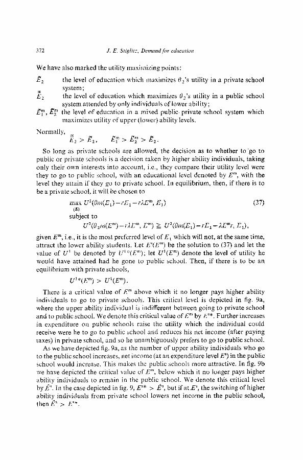
We have also marked the utility maximizing points:

4 the level of education which maximizes 0,‘s utility in a private school

&

system; the level of education which maximizes 0,‘s utility in a public school system attended by only individuals of lower ability;

&“, &” the level of education in a mixed public-private school system which maximizes utility of upper (lower) ability levels.

Normally,

Z, > E,, @>ET>B,.

So long as private schools are allowed, the decision as to whether to ‘go to public or private schools is a decision taken by higher ability individuals, taking only their own interests into account, i.e., they compare their utility level were

they to go to public school, with an educational level denoted by Em, with the level they attain if they go to private school. In equilibrium, then, if there is to be a private school, it will be chosen to

max U’(Bm(E,) - rE, - rl.E”, El) (37) (0

subject to

U2(8.p(Em)--AEm, Em) 2 U2(8m(E,)-rE,-lE”r, E,),

given E”, i e., it is the most preferred level of E, which will not, at the same time, attract the lower ability students. Let E”(E”) be the solution to (37) and let the value of U’ be denoted by U’“(Em); let U’(Em) denote the level of utility he would have attained had he gone to public school. Then, if there is to be an equilibrium with private schools,

V*(P) > U$Y).

There is a critical value of Em above which it no longer pays higher ability individuals to go to private schools. This critical level is depicted in fig. 9a, where the upper ability individual is indiflerent between going to private school and to public school. We denote this critical value of Em by ES*. Further increases in expenditure on public schools raise the utility which the individual could receive were he to go to public school and reduces his net income (after paying taxes) in private school, and so he unambiguously prefers to go to public school.

As we have depicted fig. 9a, as the number of upper ability individuals who go to the public school increases, net income (at an expenditure level E”) in the public school would increase. This makes the public schools more attractive. In fig. 9b we have depicted the critical value cf Em, below which it no longer pays higher ability individuals to remain in the public school. We denote this critical level by Es. In the case depicted in fig. 9, ES* > i?, but if at-E’, the switching of higher ability individuals from private school lowers net income in the public school, thenl? > ES*.


Although the more able make their own decision about whether to go to private schools, their decision clearly depends critically on the level of education provided in the public schools. This, in turn, depends on the voting decisions of

/ / O,-private I

1 is

Fig. 9

the majority, and in the subsequent analysis, we shall assume that the lower ability group is in the majority.

We can then consider two alternatives : the lower ability group (the majority) makes its decisions myopically, i.e., failing to take into account the reactions of the more able group, or it makes its decisions with full knowledge of the total consequences.


Myopic decision making

As in the earlier analysis of section 4, the preferences of the majority (the lower ability group) will not be single-peaked. For very low expenditure levels on public education, the more able clearly prefer going to private school; the utility of the less able clearly increases with successive increases in education. But at the critical level of expenditure in the public schools, which we denoted above by ES*, it no longer pays an individual of ability 8 1 to go to private school. As individuals of higher ability switch to the public schools, taxes rise and incomes before taxes in the public school also rise (since a larger fraction of the ‘graduates’ are higher ability, and all graduates are treated identically). The net income of the lower ability students will, at this level of education, change discreetly: the increase in taxes lowers their income, the increase in average ability of the graduates raises it. The net effect is indeterminate.

Fig. lOa-f illustrates some of the various possibilities :

(a) Preferences of lower ability are single-peaked with peak occuring at Em < ES*. In this case, the level of expenditure on education in the public schools is higher than it would have been in the corresponding private school for lower ability; on the other hand, expenditure on education in the upper ability school is normally smaller than it would have been in the pure private school system: the tax required to finance the public school has an income effect which normally would reduce the demand for education; and the higher level of expenditure on educ:a:ion for the lower ability individuals means that the required level of expenditure on education in the upper school to exclude the lower ability students is lowered.

(b) Preferences of lower ability has a single peak, with the peak occuring at ES* : ES* > I?. With myopic voting behaviour, there is no ‘equilibrium’ but the expenditure oscillates. At E slightly below ES*, the lower ability individuals vote for increases in Es, to a level at which private schools are no longer viable; when there are no private schools, when the expenditure is above ,!?, they vote for reductions in expenditure. As expenditures get lower, eventually private schools become attractive once again at the point we have denoted by I?. Thus the expenditure oscillates between J? and Es*, never settling down.

(c) Preferences are single peaked, with peak occurring at Es* < Em < I?. For expenditure levels between @ and ES*, the public schools would be mixed; some of the upper ability students would go to private school, some to public school. Although when all the upper ability individuals go to public school, net income of the lower ability is smaller than when none of them go, it may reach a peak when a fraction of the upper ability individuals go to the public school. This is the case depicted in fig. 10~.

(d) Preferences are single-peaked, with peak occurring at E > ES*. Then the equilibrium is a pure public school system; with the equilibrium expenditure being the point on the ‘pooling curve’ which maximizes the utility of the lower ability

J. E. Stiglitr, Demand for education 375

individuals. This will entail a higher level of expenditure than the lower ability would have purchased in the mixed public-private school system (and a fortiori

higher than they would have purchased in a pure private school system) but lower than the expenditure level which the able would have purchased in a private school system.

E“ +

Fig. 10. (a) Equilibrium mixed public-private school system; (b) no equilibrium with myopic voting; (c) equilibrium with mixed public-private systems (level of expenditure determined to

exclude 8,).

(e) Preferences of lower ability have two peaks, one at an expenditure lower than ES*, and one at an expenditure greater than Es*. Then there are two ‘local’ equilibria, one with a pure public school system (a single school for everyone)

376 J. E. Stiglirz, Demand/or education

and one with a mixed public-private school system. (f) Preferences of lower ability have two peaks, one at an expenditure lower

than Es and one at Es*. The two possible ‘equilibria’ have been described under (a) and (b).

(g) Preferences of lower ability have two peaks, one at an expenditure greater than Es* and one at Es*. In this case, there is only one myopic equilibrium, that with a pure public school system. The reason for this is that at ES*, the lower ability individuals, ignoring the possibility that the higher ability individuals will

t

IdI /Y-X

/’ \

/’ \ \ \

I \

I \ I

\ \

/

(f)

l4

.--. ,/’ ‘\

/ \ I \ I

\ \

/-+

\ \ \ \

/-

,/---., ’ 1’ \ ‘/ \ V \

Fig. 10. (d)-(g).

no longer find private school attractive, observe that increases in expenditure increases their income. But after voting for some expenditure level in excess of ES’::, the private sector ‘atrophies’; in the new, pure public school system, the optimal level of expenditure is at some level higher than Es*.

Which situation we are in depends critically on whether, at Es, income of the lower ability individuals rises or falls as the individuals of higher ability ‘join’ the public school system. It is more likely to rise, the larger the difference in ability.


Non-myopic voting

There are two important differences between myopic and non-myopic voting. First, the lower ability individuals know that if expenditures exceed max(ES*, g’“), private schools will not be viable, and if they fall below min(E’*, 83, a pure public school system will not be viable. Hence, in situation (b) above, they would set E” at a level slightly higher than 6’. Secondly, when there are ‘two peaks’, they can make sure that the expenditure level chosen is that at which their utility is actually highest, i.e., they decide, given the reactions of the higher ability individuals, whether, in effect, to have a pure public school system or a mixed public-private school system.

Note that while in the pure private school system, the lower ability simply choose that level of expenditure on education which maximizes their utility,

Income

private public mixed public private

private

Fig. 11

without regard to the higher ability individuals; in thiscase, the lower ability may choose a higher level of expenditure than they otherwise would have chosen - in order to attract the upper ability individuals into the public school system and to discourage a private school system - or they may choose a lower level of expenditure than they would otherwise have chosen - in order, in effect, to keep the upper ability students in private school and thus force them to pay ‘twice’ for education. (Fig. 11 provides an example of a comparison between private and mixed public-private school systems.)

5.3. Screening by examination

So far, we have focused on screening through self-selection. Perhaps the most important part of educational screening is a result of the educational process itself; that is in the course of education a great deal of information about individuals’ characteristics is produced as a by-product. Indeed, one of the ways

378 J. E. Stighr, Demandfor education

in which the educational system increases productivity is to sort out individuals into their comparative advantages, and in doing so, it obtains a great deal of information about absolute advantages.

More accurate screening means education yields a private return which differs from the social return; for in addition to the direct productivity effect of increased educational expenditure the individual is ‘separated out’ more accurately from individuals with whom he otherwise would have been grouped. If the individuals with whom he otherwise would have been grouped had a higher productivity than he, then this screening effect means the private return to screening will be negative; if the individuals with whom he would have been grouped had a lower productivity, then the private return will be positive.

There may, of course, be a ‘social’ return from sorting individuals according to their ability. Within the educational system itself screening yields a return in enabling students of different ability levels to obtain the education appropriate to their ability level. The social returns from this sorting, however, are markedly different from the private returns. The social return in screening is from not ‘wasting’ educational resources on the less able; the private return is not sharing ability rents with the less able. Private returns may be greater or less than social returns. It is clear, however, that in general in either a private or a public school system there is not likely to be an ‘efficient’ level of educational expenditure.

To see more clearly the nature of the equilibrium, let us continue with our analysis of an economy with only two ability groups. The school system puts ‘labels’ on all individuals passing through it; each individual is labelled either ‘upper ability’ or ‘lower ability’. No labelling (screening) system is perfect, so some individuals are misclassified. But an individual receives an income equal to the mean marginal productivity of those with whom he is classified.

Finally, we assume that higher levels of expenditure on education will, in general, be associated with more accurate screening.

Prioate scltools

The analysis proceeds much as in section 4.1 with two important modifications. Now, the income of individuals is a random variable, with a distribution depending on their ability, the level of education, and the mix of individuals in their school. For simplicity, we shall consider the ‘certainty equivalent’ income, and in the diagram, it is this which now becomes the vertical axis. Secondly, this certainty equivalent income is different for individuals of the two ability groups (while in the earlier analysis, all individuals going to the same school received the same income).

In fig. 12, we have drawn the ‘income’ curves for the upper ability individuals assuming that only able individuals go to the upper school (this curve is identical with that of earlier figures), and assuming that everyone goes to the same school. Similarly, we have drawn the lower ability income curves assuming that they go


to the lower ability school (again, the same as depicted in earlier figures) and assuming that everyone goes to the same school. The indifference curve of the lower ability individual tangent to his own income curve is also drawn. If some, but less than 100% of the lower ability individuals go to the lower school, then they must be on the same indifference curve. The corresponding income points of the higher ability individuals are given by the dotted line, in fig. 12, and the utility maximizing level of expenditure in the private schools is given by the tangency of the dotted line with the upper ability individual’s indifference curve. In this case, the equilibrium expenditure on education in the ‘upper school’ is less than in the private school system with no screening-by-examination.

IncOme 0, m(E)-E

Fig. 12

Public schools

The major alterations in our analysis of the equilibrium in the public school and mixed public-private school systems are: (a) Es*, the maximum value of expenditure on public schools at which private schools are still viable, is lowered; since even the public schools are partially differentiating between the more and the less able, the expected utility of the more able in going to public school is increased. (b) The level of expenditure in the public schools, when both groups go to public school, when it is not equal to ES*, is reduced, for two reasons - (i) the expected real return to education (from.‘skill acquisition’) is lower for the lower ability than it is for the population as a whole, (ii) the increased expenditure on education may increase the differentiation between the more able and the less able, and thus lower the expected income of the less able.”

Thus, the effect of screening-by-examination is to lower expenditure in public schools, and in the mixed public-private school system, to lower it in the private

loThis factor need not be very important; the less able may design a school system with only limited screening, and, more important, the accuracy of screening need not increase with expenditures.

380 1. E. Stiglitz, Demandfor education

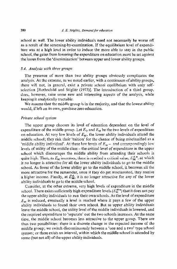
school as well. The lower ability individuals need not necessarily be worse off as a result of the screening-by-examination. If the equilibrium level of expenditure was at a high level in order to induce the more able to stay in the public school, the gains from lowering the expenditure on education must be set against the losses from the ‘discrimination’ between upper and lower ability groups.

5.4. Analysis with three groups

The presence of more than two ability groups obviously complicates the analysis. At the extreme, as we noted earlier, with a continuum of ability groups, there will not, in general, exist a private school equilibrium with only self- selection [Rothschild and Stiglitz (1973)]. The introduction of a third group, does, however, raise some new and interesting aspects of the analysis, while keeping it analytically tractable.

We assume that the middle group is in the majority, and that the lowest ability would, if left on its own, purchase zero education.

Private school system

The upper group chooses its level of education dependent on the level of expenditure of the middle group. Let E, and EM be the two levels of expenditure on education. At very low levels of EM, the lower ability individuals attend the middle school; they risk their ‘tuition’ for the chance of being misclassified as a ‘middle ability individual’. At these low levels of EM - and correspondingly low levels of utility of the middle class - the critical level of expenditure in the upper school which discourages the middle ability from attending their schools is quite high. Then, as EM increases, there is reached a critical value, Eg*, at which it no longer is attractive for all the lower ability individuals to go to the middle school. As fewer of the lower ability go to the middle school, it becomes all the more attractive for the remainder, since if they do get misclassified, they receive a higher income. Finally, at E,, “SL it is no longer attractive for any of the lower ability individuals to go to the middle school.

Consider, at the other extreme, very high levels of expenditure in the middle school. There exists sufficiently high expenditure levels (I$*) that it does not pay the upper ability individuals to run their own schools. As the level of expenditure EhI is reduced, eventually a level is reached where it pays a few of the upper ability individuals to found their own school. But as upper ability individuals leave the middle school, the utility level of the middle individuals is lowered, and the required expenditure to ‘separate’ out the two schools increases. At the same time, the middle school becomes less attractive to the upper group. There are thus two possibilities: there is a discrete change in the expected income of the middle group; we switch discontinuously between a ‘one and a two’ type school system; or there exists an interval, within which the middle school is attended by some (but not all) of the upper ability individuals.


Thus expected utility of the middle class - taking into account the reaction of the upper and lower classes - may have several peaks: there may be a low level peak, when the middle school is also attended by individuals of lower ability; since a large fraction of educational expenditures are then unproductive, the ‘optimal level of expenditure’ in the school is very low; there may exist another peak in the interval during which only the middle ability attend the middle school, or the peak may be at the boundaries, Eg* or EC*. Finally, there may be a high level peak when the school is attended by both the upper and middle ability individuals (fig. 13).

As in our earlier discussion, a competitive equilibrium may not exist; when it does, the nature of the equilibrium depends to a large extent on the degree of myopia concerning the reactions of the one group to any action of the other group. For simplicity, we consider only the case where each side takes the level

UM

school attended

middle classes

attended by middle and upper classes

EM Fig. 13

of expenditure of the other group as given. In our earlier discussion, we traced out the curve giving E,’ as a function of EM. It is obviously in the interests of the middle group to be grouped with the upper group, so long as the upper group’s expenditure is not too high. The only way to ensure this is to set EM =

E,, for En < EH < I?, . For values of E, greater than the critical value, E,, the middle school chooses whatever level ofexpenditure maximizes its own utility. For values of E, below the critical value En, ‘there is a value of EM which will attract all the upper group individuals. The resulting reaction curves are depicted in fig. 14.

As depicted, there is an indeterminacy in equilibrium, with a single private school attended only by upper and middle students (but not by lower ability students). Other configurations are easily characterized.

More generally, if some individuals do not have perfect knowledge of their abilities, or if they differ in their attitudes towards risk, then the expected income

F

382 J. E. Stij$itz, Demand/or educntiorl

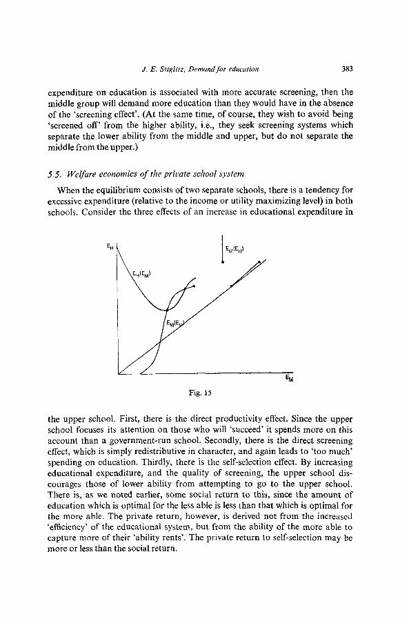
of the middle group will be a continuous function of EM, the reaction functions may take on more complicated shapes, and multiple equilibria for the two school systems may arise. Assume that the majority within each group are risk neutral and are certain of their abilities. Each school is designed to maximize the expected net incomes of the respective group for which it is designed. Expected net income of a person going to the upper school who is of the higher ability is a function of the level of expenditure in both schools,

WHH = W-(E,, EM). Similarly

WMM = WMM(EH, EM).

Fig. 14

The higher school chooses EH given EM to maximize W”” and similarly for the school designed for the middle group. The reaction functions may take on a variety of forms. Fig. 15 illustrates a case where they may intersect several times.

There is thus a low expenditure level equilibrium and a high expenditure level equilibrium: in the latter, the more able spend a great deal on education to separate themselves off from the less able, while the less able spend a great deal to attract more of the more able. One of the equilibria may be Pareto Inferior.

Public and mixed public-private SCJ~OOJS

The only modification to our earlier analysis of public and mixed public- private schools arises from the fact that the lower group cannot be excluded from the public schools; since the lower group does not pay tuition, they will always face no risk in attempting to pass the ‘screening system’. If the middle group wishes to separate itself off from the lower group, it either has to opt for a private school system or have sufficient screening-by-examination. If additional

J. E. Stigli/z, Demand for education 383

expenditure on education is associated with more accurate screening, then the middle group will demand more education than they would have in the absence of the ‘screening effect’. (At the same time, of course, they wish to avoid being ‘screened off’ from the higher ability, i.e., they seek screening systems which separate the lower ability from the middle and upper, but do not separate the middle from the upper.)

5.5. Welfare economics of the private school system

When the equilibrium consists of two separate schools, there is a tendency for excessive expenditure (relative to the income or utility maximizing level) in both schools. Consider the three effects of an increase in educational expenditure in

EM

Fig. 15

the upper school. First, there is the direct productivity effect. Since the upper school focuses its attention on those who will ‘succeed’ it spends more on this account than a government-run school. Secondly, there is the direct screening effect, which is simply redistributive in character, and again leads to ‘too much’ spending on education. Thirdly, there is the self-selection effect. By increasing educational expenditure, and the quality of screening, the upper school discourages those of lower ability from attempting to go to the upper school. There is, as we noted earlier, some social return to this, since the amount of education which is optimal for the less able is less than that which is optimal for the more able. The private return, however, is derived not from the increased ‘efficiency’ of the educational system, but from the ability of the more able to capture more of their ‘ability rents’. The private return to self-selection may be more or less than the social return.

384 J. E. Sfiglilz, Demand for education

A similar analysis applies to the lower (middle) school. It is obviously not in the interests of those of lower ability to have extensive screening (which separates them from the more able). Although the social return to self-selection is positive, the private return to those of lower or middle ability may be negative. By increasing the level of educational expenditures they are, however, able to attract those of higher ability who are less sure of their abilities and more risk averse. This again leads to some presumption of excess spending even in the lower (middle) school. When it is publicly financed, there is a further incentive for excess spending, since now the costs for the lower school are borne by the population as a whole. On the other hand, the increased tax burden if the upper ability individuals switch from private to public schools may lead to a lower level of expenditure.

Stiglitz (forthcoming) has investigated in some detail the publicly supported comprehensive school, in the case of a continuous distribution of abilities. It was shown that, for fairly accurate grading systems, the majority voting equilibrium entails both a higher level of educational expenditure and a larger coefficient of variation in incomes than would be the case if net national product were maximized, provided the median of the distribution is greater than the mode, as in the lognormal distribution.

More generally, what is clear is that neither the private nor the public majority voting school systems does as well as a ‘benevolent despot’ might have done. Neither has any clear optimality properties; whether one is preferable to another depends not only on political and value judgements but even on narrow efficiency grounds, the comparison requires detailed knowledge of production functions, ability distributions, the structure of the educational system and how screening and skill acquisition are related, etc.

6. Concluding comments

This paper has attempted to trace out the determination of the equilibrium level of education in private, mixed public-private school systems, and public school systems, viewing education separately as a public consumption good, a private capita1 good, a private consumption good and a source of information about individual’s abilities. In each case, we observed that the equilibrium level was not likely to be at the ‘efficient’ level; in some cases as when education is viewed as a pure public good there was some presumption for the equilibrium to be an undersupply. In other cases there was some presumption for excessive expenditures on education. The relative importance of these various considerations is, I am sure, a subject on which we can have much debate.

References

Arrow, K., 1973, Higher education as a filter, Journal of Public Economics 2,193-217.

J. E. Stiglitr, Demand for education 385

Rothschild, M. and J.E. Stiglitz, 1973, Equilibrium in competitive insurance markets; the economics of imperfect information, Paper presented to the Oslo Meetings of the Econo- metric Society, Sept.

Spence, M., 1973, Job market signalling, Quarterly Journal of Economics 87,355-379. Stern, N., 1973, Welfare weights and the elasticity of the marginal valuation of income, mimeo.

(St. Catherine’s College, Oxford). Stiglitz, J.E., forthcoming, The theory of ‘screening’ education and the distribution of income,

American Economic Review. Stiglitz, J.E., 1972, Education as a screening device and the distribution of income, mimeo.

(Yale University, New Haven, Conn.). Stiglitz, J.E., 1974, The pure theory of local public goods, I.E.A. Conference (Turin).

THE DEMAND FOR EDUCATION IN PUBLIC AND PRIVATE …

Documents

Transcript of THE DEMAND FOR EDUCATION IN PUBLIC AND PRIVATE …