Income and Wealth E�ects on Private-Label Demand: Evidence

From the Great Recession∗

Jean-Pierre Dubé

NBER and Booth School of Business

University of Chicago

Günter J. Hitsch

Booth School of Business

University of Chicago

Peter E. Rossi

Anderson School of Management

UCLA

December 2016

forthcoming Marketing Science

Abstract

We measure the causal e�ects of income and wealth on the demand for private-label products.Prior research suggests that these e�ects are large and, in particular, that private-label demandrises during recessions. Our empirical analysis is based on a comprehensive household-leveltransactions database matched with price information from store-level scanner data and wealthdata based on local house value indices. The Great Recession provides a key source of thevariation in our data, with a large and geographically diverse impact on household incomesover time. We estimate income and wealth e�ects using �within� variation of income, at thehousehold level, and wealth, at the zip code level. Our estimates can be interpreted as incomeand wealth e�ects consistent with a consumer demand model based on utility maximization. Weestablish a precisely measured negative e�ect of income on private-label shares. The e�ect ofwealth is negative but not precisely measured. However, the estimated e�ect sizes are small, incontrast with prior academic work and industry views. An examination of the possible supply-side response to the recession shows only small changes in the relative price of national-brandand private-label products. Our estimates also reveal a large positive trend in private-labelshares that predates the Great Recession. We examine some possible factors underlying thistrend, but �nd no evidence that this trend is systematically related to speci�c private-labelquality tiers or to the overall rate of private-label versus national-brand product introductions.

∗We are grateful to Nikhil Agarwal, Selin Akca, Ron Borkovsky, Bart Bronnenberg, Greg Crawford, Avi Goldfarb,Ernan Haruvy, Emir Kamenica, Ryan Kellogg, Xueming Luo, Puneet Manchanda, Eleanor McDonnell Feit, KanishkaMisra, Sridhar Moorthy, Matt Osborne, Brian Ratchford, two anonymous reviewers, and the Associate Editor atMar-keting Science for helpful comments and suggestions. We also bene�ted from the comments of seminar participants atthe 2014 Marketing Insights at Chicago Booth Conference, the 2015 QME Conference, the 2015 Marketing and Eco-nomics Summit, the European Commission, UC Davis, the University of Michigan, Temple University, the Universityof Toronto, UT Dallas, and the University of Zurich. Gentry Johnson and James Sams provided excellent researchassistance. We also bene�tted from the �nancial support of MSI Research Grant #4-1765 and a grant from the IGMat the Chicago Booth School. All correspondence may be addressed to the authors at the Booth School of Business,University of Chicago, 5807 South Woodlawn Avenue, Chicago, IL 60637; or via e-mail at jdube@chicagobooth.eduor guenter.hitsch@chicagobooth.edu or perossichi@gmail.com.

1

1 Introduction

Private-label products are an important component of retail strategy and correspondingly a concern

for national-brand manufacturers. A growing area of interest is the extent to which the demand for

private-label products is sensitive to income and wealth. A key question is whether private-label

products are inferior goods, such that household demand for private-label products decreases in the

level of income or wealth.

The question of income and wealth e�ects on private-label demand has received renewed atten-

tion during and after the Great Recession (the NBER dates this recession from December 2007 to

June 2009). Some industry sources (see, for example, Nielsen 2011) have claimed that US private-

label shares increased by over two percentage points on a base of about twenty percent during

the recession. Some industry insiders attributed this increase to the recession. According to Mike

Moriarty, a partner at AT Kearney: �Generally speaking, if a recession lasts more than 6 months,

retailers can expect to see more of a switch to private labels� (Wong 2008). Describing a recent

private-label purchase survey, Chris Urinyi, CEO of Lightspeed Research, concludes: �The economic

recession is causing an increase in private-label purchasing, a trend that our survey results show

is unlikely to change after economic recovery� (Frank 2010). Professor Jan-Benedict Steenkamp

reports: �We've done studies spanning decades, and what we document, very clearly, is that private

label grows a lot in recessions� (Hammerbeck 2008). Quelch and Harding (1996) assert that �...

private-label market share generally goes up when the economy is su�ering and down in stronger

economic periods.� Some prominent academic work on private-label demand over the business cycle

supports the notion that private-label demand increases due to a decline in income or wealth. For

example, Lamey, Deleersnyder, Dekimpe, and Steenkamp (2007) estimate that a one percent decline

in real per capita GDP leads to a permanent increase in the private-label-share annual growth rate

of 1.22 percent.

The large income e�ects thought to characterize private-label demand and the evidence on the

growth of the overall private-label share during the Great Recession suggest that there may also

have been a supply response. For example, national-brand manufacturers may have lowered the

e�ective price of national-brand products relative to private-label products. Similarly, retailers

that experienced an increase in the demand for private-label products may have increased private-

label prices. Other supply responses such as the introduction of new private-label products and/or

changes in the quality of private-label products are also a possibility.

The goal of this paper is to provide causal, demand-based estimates of household-level income

and wealth e�ects on private-label demand as well as to provide evidence on the supply response

(if any) to the experience of the Great Recession. To achieve this goal we utilize household-level

transaction data for a comprehensive set of private-label and national-brand products as well as

information on the supply side based on store-level scanner data. We use household data from the

Nielsen Homescan panel to examine how income and wealth a�ect private-label demand. These

data contain detailed purchase records of more than 130,000 households' CPG shopping histories

across all U.S. retailers in more than one thousand food and non-food product categories. The data

2

include demographic information including income and employment status. We measure household

income as an annual �ow variable.

To measure wealth, we supplement the Homescan data with Zillow home value indices that are

available at the local ZIP code level. Housing represents a large portion of household net worth

(Iacoviello 2011) and changes in housing net worth explain most of the cross-sectional variation in

household net worth during the Great Recession (Mian, Rao, and Su� 2013). We also supplement

our data with Nielsen's Retail Measurement System (RMS) database to measure the private-label

and national-brand price levels that households face.

Our data cover the years 2004-2012, which include substantial data prior to and after the Great

Recession. No other recession since World War II experienced as large a decline in real GDP and

increase in unemployment as the Great Recession.1 The Great Recession is also the macroeconomic

event associated with the largest impact on income and wealth since high-quality household panel

data and store-level scanner data have been available. Our empirical strategy relies on two crucial

features of the Great Recession. First, there were large changes in income and wealth over a short

time horizon. Second, these income and wealth changes varied considerably across geographic areas

and households.

The �rst major goal of our analysis is to establish a causal e�ect of income and wealth on

private-label spending. We �nd that the aggregate private-label share increased by approximately

one percentage point during the Great Recession. However, much of this increase appears to be

part of a long-term trend that pre and post-dates the Great Recession. Even a deviation from this

trend or a level shift in the private-label share need not indicate a causal e�ect, but could represent

a change in private-label spending that would have occurred irrespective of the incidence of the

Great Recession. Relying purely on the time-series variation in the data, we cannot establish causal

income and wealth e�ects without making strong assumptions about the counter-factual private-

label spending patterns in the absence of the Great Recession. Similarly, the estimated income and

wealth e�ects obtained purely from the cross-sectional (between) variation in private-label spending

across households need not be causal. A selection bias would arise if, for example, households who

choose careers with relatively high incomes also have systematically stronger preferences for branded

products than households who choose careers with low incomes.

To establish causality, we exploit the panel structure of our data. We analyze the within-

household variation in private-label shares associated with within-household changes in income and

wealth, controlling for other factors including an overall trend in private-label shares. The main

identifying assumption is that conditional on all other controls, including an overall trend, within-

household changes in income and wealth are as good as randomly assigned or exogenous. The

identifying assumption would be violated, for instance, if during the recession income and wealth

systematically decreased for those households or in those areas with a systematically above average

private-label share trend. However, we �nd no systematic evidence of a local (or household-speci�c)

1Unemployment reached a slightly higher level in the 1981/1982 recession, but the increase in unemployment wassmaller than during the Great Recession.

3

correlation between the pre-recession trend in private-label shares and the change in income, wealth,

and unemployment during the recession.

We estimate a negative e�ect of income and wealth on household-level private-label shares, which

is consistent with industry views and some prior academic work. However, the e�ect sizes are one

or two orders of magnitude smaller than the estimates in some of the prior academic work once we

control for persistent household di�erences and time trends. In contrast to these small e�ect sizes,

the overall trend in the private-label share is large and increased during the recession.

The estimated income and wealth e�ects can be interpreted as causal subject to the identifying

assumption stated above. However, in general these causal estimates will capture di�erent mecha-

nisms by which private-label demand was a�ected. First, income and wealth have a direct e�ect on

private-label purchasing behavior as predicted by the theory of consumer demand. Second, income

and wealth changes may a�ect the supply side, in particular the retail prices of national-brand and

private-label products, creating an indirect e�ect on private-label demand. The second major goal

of our analysis is to distinguish between these direct and indirect e�ects of income and wealth.

We estimate a demand model, allowing us to test if private-label products are inferior goods,

which is not possible based on a private-label-share model only. We assume a demand model based

on multi-stage budgeting across product groups. In the upper-level stage, households allocate their

budgets across di�erent products groups, including CPG (consumer packaged goods), the group that

contains the products in our analysis. In the lower-level stage, households allocate the CPG budget

across private-label and national-brand products. We model lower-level demand using an AIDS

speci�cation with household-level private-label shares as the dependent variable along with controls

for private-label and national-brand prices and the overall price levels of the di�erent upper-level

product groups.

To estimate the demand model we construct private-label and national-brand price indices that

are customized to each household's expenditure patterns across categories using the RMS scanner

data. We �nd that changes in the national-brand/private-label price ratio that households face are

correlated with household-level changes in income and wealth. Hence, the demand estimates could

be subject to omitted variables bias if we did not include price controls. The correlation between

the price ratios and income and wealth is not perfect, however, and hence disentangling the direct

income and wealth e�ects on private-label demand from the indirect e�ect of income and wealth

through their e�ect on prices is possible.

Our demand estimates, which control for private-label and national-brand price levels, show a

negative direct income e�ect on private-label shares. Hence, the negative causal income e�ect in

our initial analysis is robust to controls for prices. The estimated wealth e�ect is negative but not

statistically di�erent from zero.

To test if private-label products are inferior goods we predict the (total) income elasticity of

private-label demand based on the elasticities of the private-label share and CPG spending with

respect to income. We �nd that the point estimate of the income elasticity of private-label demand

is positive. A 95 percent con�dence interval includes negative and positive values, hence we can

4

neither rule out that the private-label product group is an inferior good nor a normal good. In

either case, the con�dence interval indicates that the income elasticity of private-label demand is

small.

Our �ndings of small income and wealth e�ects on private-label demand are in stark contrast

to some prior academic work. In contrast to these small e�ect sizes, our household-level estimates

reveal an economically large positive trend in the private-label share of 0.45 share points per year.

On the supply side, we �nd no evidence of a reduction in the relative price of national-brand

versus private-label products either during the recession or after. The national brand/private label

ratio remained constant during the recession and increased slightly afterwards. We also investigate

whether the private-label share trends di�er by quality tiers, de�ned based on private label/national-

brand price ratios. Both academic researchers (ter Braak, Geyskens, and Dekimpe 2014) and

industry practitioners have called attention to the growth in high-quality private-label products.

However, our analysis does not reveal a stronger demand trend among higher-quality private-label

products compared to lower-quality private-label products. We also examine new private-label and

national-brand product introductions to see if these coincide with the strong demand trend and

�nd that private-label and national-brand product introductions are remarkably stable during the

sample period from 2006-2010.

The plan of the paper is as follows. After describing our household panel sample, we provide some

descriptive analysis to document the extent of aggregate trends in private-label shares in Section 4.

We argue that this aggregate analysis cannot provide causal estimates of the impact of income or

wealth changes on private-label demand without strong assumptions on the counter-factual share

outcomes. For this reason, we base our analysis on household-level data in Section 5. To construct

estimates of the income e�ect on the demand for private label, we must construct a valid demand

system and estimate this system using prices of national brand, private label and other products.

Section 6 provides such estimates. Finally, we investigate various possible supply-side explanations

for private-label-share growth in Section 7.

2 Literature

While academics have documented suggestive evidence that economic recessions are associated with

private-label-share growth (e.g. Quelch and Harding 1996; Ang, Leong, and Kotler 2000), there are

few academic studies that rigorously test for income and wealth e�ects in private-label demand.

Hoch and Banerji (1993) were among the �rst to draw attention to a strong negative correlation

between disposable income and the private-label share using annual time-series data from the U.S.2

Lamey, Deleersnyder, Dekimpe, and Steenkamp (2007) �nd a similar countercyclical pattern between

GDP growth and private-label demand using time-series analysis of national, annual private-label

shares for four di�erent countries. They conclude that �...the aggregate business cycle contributes

to long-term private-label success.� In a meta-analysis of annual U.S. time-series data for 106 CPG

2See Figure 1, p. 59.

5

categories, Lamey, Deleersnyder, Dekimpe, and Steenkamp (2012) recon�rm that the private-label

share is countercyclical. They also �nd that some of the cyclicality is moderated by a supply-side

response, especially the pro-cyclicality of national-brand price promotions. Based on their estimates,

Lamey, Deleersnyder, Dekimpe, and Steenkamp (2007) conclude that for each 1 percent decline in

real per capita GDP, there will be a permanent increase in the annual growth rate of the private-label

expenditure share of 1.22 percent.3 In the recent Great Recession, real GDP per capita declined by

5.5 percent. Correspondingly, the model in Lamey, Deleersnyder, Dekimpe, and Steenkamp (2007)

predicts that the private-label share will double within 10 to 11 years after the recession and thus

represents the largest estimated e�ect of income on the aggregate private-label share.

A related literature has used purely cross-sectional variation in household characteristics to study

the sources of heterogeneity in tastes for private label products. Most of this literature uses survey

data (e.g. Murphy and Laczniak, 1979; Rosen, 1984; Batra and Sinha, 2000; Ailawadi, Neslin, and

Gedenk, 2001). Studies using consumer purchase panel data also typically rely on cross-sectional

variation in household characteristics (e.g. Erdem, Zhao, and Valenzuela, 2004; Hansen, Singh, and

Chintagunta, 2006; Ailawadi, Pauwels, and Steenkamp, 2008; Bronnenberg, Dube, Gentzkow, and

Shapiro, 2014).4 The evidence in these studies is mixed. Cross-sectional di�erences across consumers

may not provide a reliable source of variation to test for income e�ects because of selection. Testing

for selection bias is di�cult and suitable instruments are not immediately obvious.

We contribute to this literature by using household-level panel data. The sample period includes

several years pre-, during- and post-Great-Recession. We exploit geographic di�erences in the

magnitude of the income and wealth shocks of the Great Recession to identify a causal e�ect of

income and wealth on the private-label share.

Nevo and Wong (2015) use a subset of our household panel data to study the e�ects of the Great

Recession on overall household grocery shopping behavior. They �nd a large increase in the private-

label expenditure share for CPG food categories of 1.5 to 2 percentage points during the recession.

We use a longer time frame spanning 2004 to 2010, revealing a large trend in the private-label share

that pre-dates the recession and explains much of the increase in the private-label share during the

recession. We also conduct an extensive analysis of store-level price data for a large number of U.S.

supermarkets. We �nd that the national-brand/private-label price ratio increased slightly during

the recession, which would imply an increase in the returns to shopping for private-label products,

in contrast with the �ndings in Nevo and Wong (2015).

In another related paper, Stroebel and Vavra (2016) use the same household panel data matched

with retail prices in some product categories and local home values. They estimate large elasticities

of retail prices with respect to local home values ranging from 15 to 20 percent. They attribute this

relationship to changes in mark-ups as opposed to changes in marginal costs. They also �nd that

rising home values are correlated with lower private-label expenditure shares for home owners and

increased private-label expenditure shares for renters. However, they do not control for retail prices

3Formally, this is the annual impact of per capita GDP on the steady-state growth of the private-label share.4Some authors have used aggregate sales and market share data correlated with regional di�erences in demograph-

ics (Hoch and Banerji 1993; Raju, Seethuraman, and Dhar 1995; Dhar and Hoch 1997)

6

in the regression and hence one cannot interpret these estimates as wealth e�ects on demand. In

our analysis, when we control for local retail price levels, we estimate a negative wealth e�ect that

is small and statistically insigni�cant. We also �nd that while higher home values lead to a lower

private-label share in CPG expenditures, they also lead to a higher overall CPG expenditure level

and correspondingly a positive although statistically insigni�cant income elasticity of private-label

demand. Therefore, in spite of the negative e�ect on private-label expenditure shares, we cannot

reject that the private-label product group is a normal good.

More recently, Cha, Chintagunta, and Dhar (2015) conduct a descriptive analysis of household

shopping patterns during the recession. They document several interesting facts, such as a growth

in spending on food categories and a shift in shopping trips towards lower-price store formats. While

they do study private label purchasing behavior during the recession, the analysis does not address

the economics of inferior goods and the paper does not test for income or wealth e�ects.

Our work is also related to the broader literature studying consumer demand for CPG products

over the business cycle (e.g. Gordon, Goldfarb, and Li 2013, van Heerde, Gijsenberg, Dekimpe, and

Steenkamp 2013, Kamakura and Du 2012, Estelami, Lehmann, and Holden 2001). Unlike previous

work, we have access to a much more comprehensive scope of product categories spanning all of the

CPG industry.

A related literature has also measured the income e�ects on CPG demand by exploiting large

shocks to gasoline prices. Gicheva, Hastings, and Villas-Boas (2010) �nd that lower-income house-

holds substitute towards promotional CPG items in response to large shocks to gasoline prices.

Similarly, Ma, Ailawadi, Gauri, and Grewal (2011) �nd that gasoline price shocks have much larger

e�ects on consumer's substitution towards promotional items than towards private label products.

Therefore, as with our results herein, they do not �nd evidence of large income e�ects on private

label demand.

3 Data

Our primary source of data is the Nielsen Homescan household panel. This panel provides us with

information on shopping trips and items purchased in these trips for a large number of households

over a period of time that extends before and after the Great Recession. To control for prices we

use information from the Nielsen RMS (Retail Measurement Services) scanner data set. To measure

housing wealth we use data from Zillow Inc. on housing values by ZIP code and month. In some of

our analysis we also employ U.S. Bureau of Labor Statistics unemployment data that is available

by county and by month. Below we discuss each data source in detail and provide information on

how we cleaned and assembled the data.

3.1 The Nielsen Homescan Panel

The Nielsen Homescan data is available to academic researchers through a partnership between the

Nielsen Company and the James M. Kilts Center for Marketing at the University of Chicago Booth

7

School of Business.5 The raw data include the purchase decisions of 132,326 households who make

over 500 million purchases during more than 88 million shopping trips between 2004 and 2012. To

collect these data, Nielsen instructs households to use an optical scanner in their homes to scan

the barcodes of each of the UPC-coded CPG (consumer packaged goods) items that they purchase

during trips to supermarkets, convenience stores, mass merchandisers, club stores and drug stores.

Details on the strati�ed sampling methodology employed by Nielsen to promote representativeness

of the Homescan panel can be found in Kilts Center for Marketing (2013). A key advantage of

the Homescan panel data set is that it includes all US retailers including mass merchants such as

Walmart who do not o�er their data for syndication.

For each purchased product we observe the date, the Universal Product Code (UPC), the price

paid, an identi�er for the chain in which the purchase was made, and several attributes of the

product itself including brand name and pack size. The purchases cover over 3,198,950 unique

UPC's6 from 1301 Nielsen product modules that represent the di�erent product categories across

departments: Health and Beauty, Dry Grocery, Frozen Food, Dairy, Deli, Meat, Fresh Produce,

Non-Food, Alcoholic Beverages and General Merchandise. Using the 2009 Consumer Expenditure

Survey, we estimate that the Homescan products represent approximately one quarter of the average

annual household expenditures.7

When analyzing private-label spending, we drop all the modules from the General Merchan-

dise, and Alcoholic Beverages departments. These modules contain products that are frequently

purchased in store formats that are not tracked in the Nielsen RMS data, for example printer car-

tridges and automotive motor oil. Moreover, many of these modules have limited or no private-label

o�erings.

We used several procedures to �lter out some households who did not remain in the panel for a

reasonable length of time or appeared inconsistent in their purchase records. Speci�cally, we applied

the following �lters to the raw household data:

(i) Each panelist must be in the data for at least six months.

(ii) Each panelist must average at least three trips per month.

(iii) A panelist may not have a gap of six months or more in their purchase records.

We also removed a very small number of transactions with unusually large or small prices. Speci�-

cally, we �ltered out any transaction whose recorded purchase price for a speci�c product was more

than four times the median price or less than one fourth of the median of all transactions (across

all households) for that product. We also removed any products purchased less than twenty-�ve

5http://research.chicagobooth.edu/nielsen/6UPC's are unique to a speci�c product at any given moment in time but can be re-assigned to di�erent products

over time. Hence, the Kilts Center created a UPC version identi�er for each product based on four �core� productattributes, product module code, brand code, multi-pack size, and pack size (volume). Combining the UPC andversion identi�ers we can uniquely identify each product in the data over time.

7In the 2009 CEX data, the categories �food at home,� �alcoholic beverages,� �personal care products and services,�and �tobacco products and smoking supplies� which are closest to those measured in the Homescan panel have totalCEX spending of $5,164,000. Overall CEX spending is $19,043,000.

8

times in the whole data set. Finally, we only retained those product modules present in all years

in the Homescan data. Table 1 summarizes the number of panelists, number of trips, number of

transactions, and the total expenditure across all Homescan households by year. We show both

the summary statistics for the whole data set, indicated as �Raw,� and the summary statistics for

the data obtained after applying the �lters. When applying the �lters we retain 86 percent of all

households and 85 percent of all expenditures.

The data also contain annual survey information for all Homescan households. The survey pro-

vides self-reported information on demographic characteristics such as income, education, race, and

age of the household heads. The survey also reports information about household composition,

home ownership, and where the households live. Households report their income bracket, a dis-

cretization of the income variable into twenty bins. The raw Homescan data are not representative

of the U.S. population at large. Therefore, Nielsen provides sampling weights (projection factors)

that can be used to make the raw sample representative of the populations in the whole U.S. and in

61 geographies along nine demographic variables.8 These weights are computed annually. In Table

2, we compare the raw (unweighted) marginal distributions of age, education and income from the

2011 Homescan survey to the 2010 Census. Compared to the Census data our sample is slightly

older, somewhat more educated, and the income distribution is attenuated in both tails. However,

there is a substantial overlap in the distributions of the demographic variables between our sample

and the Census data. In the key parts of our empirical analysis, we employ regression methods that

control for household demographic factors. As long as the Homescan and Census distributions of

these demographics variables overlap, our regression methods will not require any adjustment to the

data to re�ect concerns of lack of representativeness in demographics. In other parts of the empirical

analysis, where we analyze aggregate private-label expenditure shares, we use the sampling weights

provided by Nielsen to make the predictions representative at the national level.

We will employ an estimation strategy that relies on within-household income variation over

time to estimate the causal e�ect of income on private-label demand. Measuring the exact timing of

income changes is hence crucial. Nielsen conducts the household surveys during the fall of year t−1

preceding the �panel year� t when the obtained demographic information is reported in the data.

In particular, at the time of the survey Nielsen asks the households to report their annual income

in the previous year, i.e. year t − 2. Therefore, for each household we match the income in panel

year t to the transaction data in year t− 2. In the parts of the analysis that rely on both purchase

and income data, we can only employ observations for households who were in the Homescan panel

for at least three years. The corresponding number of matched observations is reported in Table

1, indicated as �Income-Matched.� We retain 71 percent of all households and 62 percent of the

expenditures in the raw data. In the parts of the analysis that rely only on purchase but not income

data we use all (�ltered) observations.

8The variables are household size, income, age of head of household, race, Hispanic origin, education of male andfemale household heads, occupation of head of household, presence of children, and Nielsen county size.

9

3.2 The Nielsen RMS (Retail Measurement Services) data

The Kilts Center for Marketing also provided us with access to Nielsen's RMS (Retail Measurement

Services) scanner data. These data contain store-level unit sales and price data by UPC and week

for approximately 35,000 stores in over 100 retail chains from 2006-2011. The Kilts Center data

include the subset of stores belonging to retail chains that authorized Nielsen to release their data

for academic research purposes. Among these chains every major format is represented, including

grocery, drug, convenience, and mass merchant stores. However, the RMS sample is not a census.

For example, the largest U.S. retailer, Walmart, is not included in the RMS data.

3.3 Household wealth data

One of the most striking e�ects of the Great Recession was the steep decline in home values.

Iacoviello (2011) estimates that about one half of all U.S. household wealth is held in the form of

real estate. Mian, Rao, and Su� (2013) report that 27 percent of household net worth is held in

housing wealth and that the Great Recession reduced average housing net worth by 10 percent.

They conclude that: �... most of the cross-sectional variation in net worth is driven by variation in

net worth due to housing. The population-weighted standard deviation of the housing net worth

shock is almost 10 times larger than the standard deviation of the �nancial net worth shock.�

Similarly, Mian and Su� (2014) �nd that �... going from the 10th to the 90th percentile of change

in housing net worth distribution in the cross-section leads to a loss in non-tradable employment of

8.2%.� Thus, not only is housing a very important (if not the largest) component of U.S. household

wealth, but changes in house prices drive most of the change in wealth both across households and

over time for the same household. Our estimates of the e�ect of wealth on private-label demand

depend only on the changes in wealth over time and across households, not on the wealth levels.

Even if household-level �nancial wealth data were available (which it is not), the addition of such

data would primarily a�ect the level, not the change in wealth that is used to identify the wealth

e�ect on private-label demand.

We use Zillow Inc.'s Home Value Index to measure home values and thus housing wealth at the

ZIP code level. ZIP codes represent small, localized housing markets. We emphasize that individual

home values are not observed, except for the tiny fraction of homes for which market transaction

prices can be measured in any given time period (in our case, one month). Instead, researchers

as well as the actual home owners themselves must estimate individual home values based on the

available sparse market transaction data and property characteristics. This justi�es our assumption

that most of the change in individual home values over time is captured by the change in the overall

home values in the local housing market as captured by the local Zillow index. As discussed in the

previous paragraph, our wealth e�ect estimates rely only on such changes in housing wealth, not

individual housing wealth levels.

Should we be concerned about measurement error because we do not observe individual home

values? First, note that property level estimates will typically have higher measurement error than

ZIP code level estimates. Second, homeowners are likely to base their home value predictions on

10

local trends in home values. Thus, we believe that we have captured most of the time-series variation

in local home values using the Zillow ZIP code level indices while keeping measurement error to a

minimum.

The Zillow home value index is computed using Zillow's �Zestimate,� an estimate of the market

value of a property. Zillow uses a proprietary formula and di�erent data sources to compute this

estimate. The data sources include property appraisals, location, market condition, and transaction

data for properties in the same geographic area. The description9 provided on the Zillow.com website

suggests a hedonic approach whereby properties are represented in terms of attributes and the local

value of each attribute is computed from transaction data. The local value of each attribute is then

used to compute the total local value of a property. The Zillow home value index is the median of

the Zestimates available for properties in a given ZIP code. To obtain a household-level measure of

housing wealth we match the home value indices to the Homescan households at the ZIP code level.

The Zillow data are one of several available measures of home values in the US, along with

the Federal Housing Finance Agency (FHFA) and Standard & Poor's Case-Shiller index. For our

purposes, the FHFA data are inadequate since they only pertain to home sales with a conforming

home mortgage. The Zillow and Case-Shiller indexes are similar (correlation of 0.95). We prefer the

Zillow data due to their more extensive geographic coverage than the Case-Shiller data, 165 versus

20 metro areas respectively.10

Zillow data have been used in the �nance literature to study the links between the real and

�nancial sectors of the economy (Mian, Su�, and Trebbi, 2015) and in economics to study the

dynamics of city growth (Guerrieri, Hartley, and Hurst 2013). The Zillow data cover many of the

most populated ZIP codes in the U.S., but do not provide complete coverage of the entire country.

Zillow coverage rates11 are above 80 percent in many U.S. states; but some important states, notably

Texas, have no coverage. Generally speaking, Zillow coverage is best in those states which have the

highest housing values (e.g California where the coverage exceeds 95 percent). In more rural states

and states with lower housing values, the coverage of the Zillow index is often below 50 percent.

The household-months in the Homescan data that we can match to a Zillow index account for about

64 percent of all expenditures in the data.

The Zillow home value indices illustrate both the severity of the Great Recession as well as its

disparate impact by region. The map in Figure 1 shows the distribution of home values in 2006

and 2009. The recession had a particularly large impact on home values in the Southwest and in

Florida. The �gure also shows the coverage issues with respect to the Zillow index: All ZIP codes

with a missing Zillow value are colored white.

9http://www.zillow.com/wikipages/What-is-a-Zestimate/10We refer the interested reader to the Zillow wikipage for a more extensive comparison of data sources:

http://www.zillow.com/wikipages/Zillow-Home-Value-Index-vs-FHFA-and-Case-Shiller/.11We de�ne coverage as the percentage of the total housing units in a region that have non-missing Zillow housing

value estimates.

11

3.4 Comparison of private-label expenditure shares in the Nielsen Homescan

and RMS data

As discussed above in Section 3.1, the Homescan sample is approximately representative of all U.S.

households in some key demographic attributes when the sampling weights (projection factors)

supplied by Nielsen are applied. However, this does not necessarily rule out that there are systematic

di�erences between the Homescan panel and the US population in the preferences for private-label

products. To examine if there are systematic di�erences in private-label demand across the two

data sources we identify three of the seven largest retailers, based on Homescan expenditures, that

are also represented in the RMS data. Figure 2 displays the time series of aggregate private-label

expenditure shares at these three chains, calculated using both the Homescan and the RMS data.

There is a small di�erence in the levels (the shares predicted using the RMS data are slightly larger),

but the Homescan and RMS private-label shares move closely together (the correlation in levels is

0.951 and the correlation in one-month di�erences in shares is 0.501). This evidence suggests that

the Homescan purchase records are largely representative of the population at large, at least with

regard to private-label purchase patterns.

4 Descriptive analysis

4.1 The basics: Private-label shares and relative prices

Most of our empirical analysis focuses on private-label expenditure shares as a measure of private-

label demand. For each household h and period (month) t we observe total spending on consumer

packaged goods products (CPG), yCPG,ht, and spending on private-label products, yPL,ht. The

private-label share is then de�ned as sht = yPL,ht/yCPG,ht. Recall from Section 3.1 that we calcu-

late the private-label shares using purchases in all departments with the exception of the General

Merchandise and Alcoholic Beverages departments. Table 3 summarizes the cross-sectional dis-

tribution of private-label shares across household-years. The mean private-label share (weighted

using the projection factors) is 19.5 in all departments and 20.66 for food products only. The

private-label shares exhibit much heterogeneity across household-years. For example, 90 percent of

all observations are in the range from 9.09 to 73.12 percentage points.

The data include both food and non-food products unlike some previous work that uses only food

products (e.g. Nevo and Wong (2015)). Private-label products are very important in many non-food

categories. Six of the top twenty product categories, ranked by total private-label expenditure, are

non-food products, including Nutritional Supplements (rank 5), Toilet Tissue (8), Cold Remedies

(10), Headache/Pain Remedies (11), Paper Towels (16), and Dog Food (19).

Private-label products o�er consumers a substantial price discount relative to national-brand

products. Based on the transaction prices in the Homescan data, the expenditure-weighted average

private label/national-brand price ratio is 0.70 across all years.12

12We �rst calculate the ratio of expenditure-weighted prices per equivalent unit in all groups of products that

12

4.2 Private-label-share evolution

The top panel of Figure 3 displays the evolution of the monthly aggregate private-label share from

2004 to 2012. The included trend curve is estimated using the non-parametric LOWESS (locally

weighted scatterplot smoothing) estimator. The recession period (December 2007 - June 2009 based

on the NBER's business cycle dating procedure) is shaded in gray. Private-label share only increased

by about one per cent during the recession period. An examination of the whole sample period from

2004 until 2012, however, reveals that this increase is part of an overall positive trend by which the

private-label share increased by about 0.45 points per year.

The smaller panels at the bottom of Figure 3 show the evolution of some important macro-

economic variables, real GDP13 in trillions of 2009 dollars, unemployment, the Consumer Con�dence

Index, and the median Zillow home value index across all ZIP codes in our sample. Focusing only

on the recession years we �nd a strong correlation between the private-label shares and the macro-

economic factors, indicating an increase in private-label demand that is associated with adverse

economic conditions. However, no such correlation is present over the whole sample period (regres-

sions of the private-label share on the economic variables yield estimates that are not statistically

di�erent from zero).

This brings us to the key question in this paper: Do adverse economic conditions have a causal

e�ect on private-label demand? Let us ignore for now that we are not controlling for other factors

that are likely to a�ect private-label demand, such as private-label and national-brand price levels

(we will control for these factors in our empirical analysis below). The top panel in Figure 3 suggests

that the increase in the private-label share during the Great Recession was unusually large relative

to the overall trend. We could use this trend-deviation as evidence for a causal e�ect of the recession

on private-label demand. Any empirical analysis that relies purely on time-series variation needs

to draw inferences about causal e�ects from such trend-deviations. This approach relies on some

very speci�c assumptions about the counter-factual or potential private-label share that would have

been observed in the absence of a recession. In particular, we need to have a strong prior on

the shape of the trend and we need to assume that any deviations from this trend are necessarily

due to the causal factors, income and wealth, in which we are are interested. Both are strong

assumptions. Our approach, outlined in detail below, follows a di�erent route and relies on cross-

sectional di�erences in the income and wealth shocks experienced by the households to establish

causality. This identi�cation strategy does not rely on any speci�c assumptions on the aggregate

trend in the private-label share.

belong to the same category and for which volume is measured in the same equivalent units. We then take anexpenditure-weighted average over these group price ratios.

13Obtained from Macroeconomic Advisors, http://www.macroadvisers.com/monthly-gdp/

13

5 The causal relationship between income, wealth, and the private-

label expenditure share

5.1 Empirical strategy

We estimate the relationship between income, wealth, and private-label demand using the following

regression:

sht = β0 + β1 log(Iht) + β2 log(Wht) + βT3 φ(t) + βT4 xht + εht. (1)

sht is the private-label share of household h in month t, and Iht is the income of household h. We

proxy for household wealth Wht using the local Zillow home value index, measured at the ZIP code

level. φ(t) is a vector-valued function of the time period t that captures time dummies and trends,

and xht is a vector of other covariates including household demographics.

Estimates of the income and wealth coe�cients in equation (1) need not represent causal e�ects,

as is always the case in observational studies. Since an experimental manipulation of household

income and wealth is not feasible, we need to be clear about the source of the variation in the

observed, non-experimentally generated income and wealth levels that allows us to establish causal

e�ects. In particular, the cross-sectional di�erences in income and wealth across households need

not be a reliable source of variation because of selection: households with high incomes may have

systematically di�erent preferences for private label versus national brands than household with

low incomes. For example, households might di�er in the importance that they attach to status

and prestige. Those households who are driven by status may choose careers associated with high

incomes and may also have a strong preference for branded products. In this case, higher incomes

will be associated with a smaller private-label share, β1 < 0, even though, in this example, there is

no causal relationship between income and private-label share. .

The selection concerns can be resolved using household �xed e�ects in (1) that control for

persistent di�erences in private-label demand across households. The income and wealth coe�cients

are then estimated using the within-household variation in income and wealth over time. To establish

causality we rely on the large variation in income and wealth due to the severity and diverse

geographic impact of the Great Recession . Figure 4 shows the large geograhic di�erences in the

impact of the Great Recession using a map of unemployment at the FIPS county level in 2006

and 2009. Similarly, Figure 1 shows a corresponding map of Zillow home value indices at the

ZIP code level. Figure 5 shows histograms of the cross-sectional distribution of the di�erences in

unemployment and (log) house values between January 2006 and December 2009. The plots indicate

large regional di�erences in the changes in unemployment and home values. While unemployment

fell in some regions, in others it increased by up to 15 percent. Similarly, home values increased in

some regions, but dropped by more than 60 percent in others. This geographical variation in the

magnitude of the recession e�ect on local economic conditions provides us with the main source of

variation to interpret the estimated income and wealth e�ects in (1) as causal.

The main identifying assumption to establish causality is that conditional on all other controls,

14

including the time trends in φ(t), within-household changes in income and wealth are �as good as

randomly assigned,� a phrase used in the causality literature. The precise meaning of this phrase

can be established using the Neyman-Rubin causal model (see Imbens and Rubin 2015 for a detailed

exposition and references). Let sht(i, w) be the potential private-label share given income level i

and wealth w. In the data we only observe the private-label share at the realized income and wealth

of household h, sht = sht(Iht,Wht). Xht is a vector of other covariates. Then the main identifying

assumption, referred to as unconfoundedness in the treatment e�ects literature, is:

sht(i, w) ⊥⊥ (Iht,Wht) | Xht, h ∀(i, w). (2)

For example, this assumption rules out that households who would have increased their share

of private-label spending irrespective of income and wealth systematically experienced an actual

decrease in income and wealth. A priori, it seems unlikely that the e�ects of the Great Recession

were particularly severe for those households with systematically above average positive trends in

private-label spending.

The unconfoundedness assumption is not directly testable. However, we can provide some

corroborating evidence that indirectly supports the assumption by examining (i) the relationship

between household or regional trends in private-label spending before the recession and (ii) changes

in income, unemployment, and wealth during the recession. For example, suppose that income

and wealth systematically fell during the recession for households or for regions with a positive

trend in private-label spending. If this trend pre-dated the recession, we would also �nd a negative

correlation between the change in income (or wealth) during the recession and the change in private-

label spending before the recession. We calculate di�erences in private-label shares between the two

periods prior to the recession and di�erences in county-level unemployment, ZIP code housing values,

and household income between two periods during the recession. The correlations are reported in

Table 4. We provide results for several time slices. For example, we correlate the change in private-

label shares between 2004 and 2006 and the change in unemployment between 2007 and 2009.

Similarly, we correlate the change in private-label shares between the �rst quarter of 2004 and the

�rst quarter of 2007 and the corresponding change in unemployment between the second quarter

of 2007 and the second quarter of 2009. We separately calculate the correlations for private-label

share changes in all categories and changes in food categories only. All correlations are small, in

most instances less than 0.03 in absolute value. We reject the null hypothesis of no correlation in

four out of thirty correlations, but with corresponding p-values that are only marginally signi�cant

of between 0.033 and 0.049. All four statistically signi�cant correlation coe�cients are negative,

which is consistent with the example of a violation of the identifying assumption (2) that we gave

above. However, the number of instances where we reject the null hypothesis is small, and these

instances are not consistent across small variations in how the time periods before and during the

recession are de�ned.14

14For example, the p-value for the correlation in the share di�erence between 2005 and 2006 and the di�erence in(log) housing values between 2007 and 2009 is 0.033, but the corresponding p-value if the share di�erence is calculated

15

5.2 Estimation results

Table 5 reports several di�erent speci�cations of the private-label share regression (1). All speci-

�cations include the log of household income and the log of Zillow home values in a household's

ZIP code. We also include a household-level unemployment dummy that may capture unmeasured

income components or permanent income components such as expectations of future income.

Column (1) contains results based on a speci�cation that pools across all households, and column

(2) contains the between-household estimates that are entirely based on the cross-sectional variation

of all variables across households. In these two speci�cations we control for DMA �xed e�ects and

household-speci�c e�ects using various demographic variables, including household composition,

education, and ethnicity. In both speci�cations the income and (housing) wealth estimates are

negative and statistically signi�cant. The income estimate in the between speci�cation implies that a

25 percent reduction in income increases the private-label share by 0.84 percentage points. Similarly,

a 25 percent reduction in housing wealth increases the private-label share by 0.35 percentage points.

In column (3) we control for persistent household-speci�c factors using household �xed e�ects.

In column (4) we add a dummy variable for all months during the Great Recession (December

2007 - June 2009 according to the NBER's business cycle dating procedure) and a dummy for the

post-recession period. In column (5) we add an overall linear trend variable, and interactions of

the trend with the recession and post-recession dummies. Speci�cally, for the recession period the

trend interaction is de�ned as follows:

trend_recessiont = I{t0 ≤ t ≤ t1} · (t− t0 + 1).

Here t0 and t1 indicate the �rst and last recession month. Using this speci�cation we can as-

sess the trend in private-label shares during the recession by the sum of the overall trend and the

trend/recession interaction. The trend interaction for the post-recession period is de�ned analo-

gously, and we can assess the trend in the periods after the recession by the sum of the overall

trend and the trend/post-recession interaction. The within-household estimates of the income,

wealth, and unemployment e�ects in columns (3)-(5) are substantially di�erent from the pooled

and between-household estimates. Also, the recession and post-recession dummies as well as the

trend variables are all statistically signi�cant. We hence focus on the estimates in column (5).

Controlling for household �xed e�ects, the income e�ect and, to a lesser degree, the wealth e�ect

are substantially smaller than the pooled and between-household estimates. The estimates imply a

0.12 percentage point increase in the private-label share for a 25 percent reduction in income, and

a 0.16 percentage point private-label share increase for a 25 percent drop in the home value. Being

unemployed increases the private-label share by 0.37 points, holding income constant. In reality,

unemployment is associated with a large drop in income. For example, if the unemployed household

retains 40 percent of her pre-unemployment income in transfer payments then the private-label

between 2004 and 2006 is 0.913. We interpret the evidence as consistent with assumption (2), even though it is nota direct test.

16

share increases by 0.75 points.

Controlling for all other factors, including the trend variables, the overall private-label share was

higher during the recession (0.32 percentage points) and also after the recession (0.48 percentage

points). The overall trend estimate is 0.0372, implying an annual 0.45 percentage point increase in

the private-label share. The level shift due to the recession, 0.32 points, is equivalent to about nine

months of the trend e�ect. Our estimates also indicate a signi�cant decline in the trend during the

post-recession period. However, we hesitate to put much emphasis on this decline because of the

limited number of sample periods in the post-recession period. In particular, the last sample year

used to obtain the results is 2010 (recall from our discussion in Section 3.1 that the income data

matched to transactions in 2010 are reported in the 2012 Homescan data, the last year currently

provided by the Kilts Center).15

In Appendix C, we report analogous estimation results for the more homogenous group of food

products only. The estimates for food products are comparable to the estimates based on all

categories.

The within-household estimates indicate a negative e�ect of income and wealth on private-label

demand. If within-household changes in income and wealth are as good as randomly assigned, then

these e�ects are causal. However, while the estimates have the expected sign, the economic signif-

icance of the estimates is small. In contrast, the overall trend is large, implying a 4.45 percentage

point increase in the private-label share over a decade.

Robustness checks

Although not reported herein, we also conducted a similar analysis using product group level data.

Nielsen has classi�ed the set of UPC's included in the analysis in Table 5 into 109 distinct product

groups, such as �Baby Food� and �Haircare and Fashion Accessory.� The product group level data

are problematic due to the high incidence of private-label shares that are zero, which is likely to

introduce attenuation bias. In contrast, based on the aggregate purchase data only 0.09 percent

of households have a private-label share that is zero. As expected, when we estimate the model

in column (5) using product group private-label shares as dependent variable we obtain slightly

smaller point estimates for the coe�cients on log income and log wealth, respectively, compared

to the results from the aggregate analysis. However, the results are very close to those from our

aggregate analysis and do not a�ect our main conclusions.

One potential concern is that a high correlation between income and home values could make it

di�cult to disentangle their respective e�ects on demand. In our estimation sample, the correlation

between log income and log wealth is 0.22. However, we �nd very little within-household correlation

between income and wealth. A regression of log income on log wealth and household �xed e�ects

generates an incremental R2 of 0.001. Running the regression using only the months during the

recession generates an even smaller R2.

15We expect to be able to obtain data for 2013 in a future revision of this paper.

17

5.3 Supply response, measurement error and permanent income concerns

The estimation results presented above are subject to some limitations that we will resolve in the

next section. First, we will provide conditions under which the regression (1) can be interpreted

as part of a valid consumer demand model. Second (and related to the �rst point), the potential

private-label shares realized for a given household may be a�ected by income and wealth changes

experienced by other households. In particular, local income and wealth changes may cause a supply-

side response whereby the prices of private-label products versus national brands are a�ected. If such

a price response occurred the SUTVA (stable unit treatment value assumption) would be violated

(see Imbens and Rubin 2015 for a discussion) and interpreting the income and wealth estimates as

causal would no longer be straightforward. We will address this issue in the next section.

We found that the within-household estimates of the income and wealth e�ects are signi�cantly

smaller than the pooled or between-estimates. This may indicate selection e�ects, whereby high

income households have di�erent preferences for private-label versus branded-products than low-

income households. One alternative explanation is that the inclusion of household �xed e�ects

potentially increases the attenuation bias due to measurement error. Another possible explanation

for the di�erences between the results which use cross-sectional variation and the results which

use within variation is that the income variation we see in the �within� results represents primarily

transient shocks to income, while the cross-sectional variation in income re�ects more of the variation

in permanent income between households. We address these concerns below in Section 6.4.

6 Estimating income and wealth e�ects on private-label demand

6.1 Demand model

In the previous section, we showed that there is an e�ect of income and wealth on the private-label

share in spending. These estimated e�ects are causal subject to our identifying assumptions, and

allow us to measure the e�ects of income and wealth on private-label purchasing behavior without

imposing a speci�c model of consumer demand. However, the exact mechanism through which

income and wealth a�ect private-label demand is not clear from this analysis. First, the theory

of consumer demand predicts that in general, income and wealth have a direct e�ect on private-

label purchasing behavior. Second, income and wealth changes may a�ect the supply-side behavior

of manufacturers and retailers, in particular the retail prices of national-brand and private-label

products. Thus, income and wealth may have an indirect e�ect on private-label demand through

its impact on relative prices. In this section, we separate these direct and indirect e�ects of income

and wealth using a proper consumer demand model. Based on a demand model we can also test

whether private-label products are normal or inferior goods.

Ideally, we would �t one of the many �exible consumer demand models that have been developed

in the marketing literature to the data, such as a mixed discrete-continuous demand model as in

Kim, Allenby, and Rossi (2002). In practice, we would have to estimate such a demand model

18

for all 953 product categories in our data, which is beyond the capabilities of the current state

of estimation of these models. Instead, we simplify the analysis by modeling a demand system

with multi-stage budgeting across commodity groups, an approach that has been used previously

in the consumer demand literature (e.g. Hausman, Leonard, and Zona 1994). The model that we

propose is consistent with utility maximization under speci�c conditions on preferences. We use

a two-stage model of demand derived from Gorman's two-stage budgeting framework (see Deaton

and Muellbauer 1980b for a general discussion). At the upper level of demand, households allocate

their total income across di�erent commodity groups. One of these commodity groups includes the

consumer packaged goods (CPG) in our data. At the lower level of the demand, households allocate

the CPG budget across national-brand and private-label products.

We emphasize that the analysis in this section is not a substitute or replacement for the analysis

in Section 5. In Section 5 we provided evidence for causal income and wealth e�ects on private-

label shares without imposing any assumptions on consumer demand. In this section we distinguish

between direct and indirect income and wealth e�ects on private-label demand subject to the speci�c

assumptions in the estimated demand model.

Upper level demand

At the upper level of the demand model households allocate their budget across K product groups.

Our upper level demand groups are de�ned as all CPG goods, General Merchandise items, and all

other non-durable goods captured in regional CPI. We focus on the CPG group and model the total

expenditure on the CPG group, yCPG, as follows:

log(yCPG) = η + δI log(I) + δW log(W ) +K∑k=1

αk log(Pk) + ν. (3)

For notational simplicity, we drop the household and time subscripts in this section. Pk is the

price index for commodity group k. Correspondingly, QCPG = yCPG/PCPG is a quantity index for

the CPG product group. The error term ν captures unobserved determinants of the total CPG

expenditure. We model upper-level demand for CPG in a manner similar to other research (e.g.

Hausman, Leonard, and Zona 1994). Unlike past work, we also include controls for prices in other

non-CPG commodity groups.

Lower level demand

At the lower level of demand, we assume PIGLOG preferences over the national-brand and private-

label product groups. Under this assumption we obtain the �Almost Ideal Demand System (AIDS)

19

of Deaton and Muellbauer 1980a with the following private-label expenditure share equation:

s =PPLQPL

PPLQPL + PNBQNB

= β + γ log

(yCPGPCPG

)+ λPL log(PPL) + λNB log(PNB) + ε. (4)

Here, PPL and PNB are price indices for the private-label and national-brand product groups. Sub-

stituting the upper level expenditure model (3) into the share equation (4) we obtain the following

speci�cation:

sPL = β + γI log(I) + γW log(W ) + λPL log(PPL) + λNB log(PNB) +

K∑k=1

αk log(Pk) + ε (5)

This share equation is a generalization of the private-label share regression (1) in Section 5. Unlike

(1) it controls for product prices and can be interpreted as a proper demand model.

A priori we expect that the assumptions behind the upper level demand system are largely innocu-

ous. However, the lower level demand system imposes some stringent restrictions on the substitution

patterns between products. In particular, the relative price of a national brand versus the price of

a private-label product in a speci�c product category a�ects substitution only through its e�ect on

the overall national-brand and private-label price indices.

6.2 Analysis of national-brand/private-label price evolution

A concern with the analysis in section 5 is that a re-adjustment of retail prices, on the supply side,

could confound any �ndings of a recession e�ect. Industry opinions about supply-side price adjust-

ments in the CPG industry during the recession have been mixed. A USDA report attributes private-

label-share growth to a �2007-2008 food price spike and 2007-2009 recession,� �nding national-brand

promotional activity to be �at during the recession16. In contrast, a Nielsen report found that �Since

the end of 2008, private brand share growth has �attened as brands stepped up their promotion

support and innovation e�orts.�17 In this section, we document the evolution of national-brand

and private-label prices during our sample period. Appendix B describes the procedure used to

construct the national-brand and private-label price indices.

Table 6 shows the average regional (DMA) national-brand/private-label price ratio by year.

These indices are obtained using regional expenditure weights instead of household-level expenditure

weights in formula (21). We �nd that national-brand prices increased relative to private-label

prices by about 2 percent in 2009 and stayed at this higher level until the end of the sample

period, 2011. Figure 6 shows the distribution of yearly percentage changes in the price ratios

(log(PNB,t/PPL,t) − log(PNB,t−1/PPL,t−1)) across regions. The graph documents some regional

variation in the evolution of national-brand-to-private-label price ratios.

16http://www.ers.usda.gov/media/187072/err129_1_.pdf17http://www.storebrandsdecisions.com/news/2012/02/07/nielsen-private-label-outlook-is-sunny

20

We next investigate if the regional di�erences in the evolution of the price ratios are related

to local economic factors. We match local (ZIP code) housing price indices and local (county)

unemployment rates to each household, and then regress the log change in the national-brand-to-

private-label price ratios on the log change in household income, the log change in house values, and

the di�erence in the local unemployment rates. We also control for year �xed e�ects. The results are

in Table 7, shown separately for price indices based on regional category expenditure weights and

household-level expenditure weights. There is clear evidence for a statistical relationship between

the change in relative national-brand/private-label prices changes in the local economic conditions.

Decreases in house values and increases in unemployment are associated with an increase in the price

of national brands relative to private-label products. Income decreases are also associated with an

increase in the national-brand relative to the private-label price; although the e�ect is statistically

insigni�cant. The e�ects are moderated by the percentage change in the local CPG price index: a

decline in the CPG price level is associated with an increase in the national-brand prices relative to

the private-label prices. In sum, our evidence suggests that deteriorating macroeconomic conditions

are associated with an increase in the national-brand prices relative to private-label prices.

There are two key implications of this analysis for the main goals of the paper. First, the

results demonstrate the potential for omitted variables bias if we fail to control for relative price

changes when estimating income and wealth e�ects on private-label demand. Second, even though

there is a clear and overall statistically signi�cant association between the price ratio changes and

changes in the economic variables, the regressions do not explain all the variation in national-brand

versus private-label prices (the R2 numbers are about 0.43 for regional price indices and about 0.16

for household-level price indices). Consequently, we can still distinguish between a direct e�ect of

income and wealth on private-label demand and an indirect e�ect through relative prices.

6.3 Lower level demand (AIDS private-label share system) results

We present the lower level demand estimates for the AIDS private-label share equation (5) in Table

8. Column (1) contains our preferred speci�cation that we used to test for causal income and wealth

e�ects in Section 5. This speci�cation includes household �xed e�ects, recession and post-recession

dummies, and trend variables. In column (2) we add the household-level price indices for national-

brand and private-label products and a price index for the entire CPG product group. We �nd that

the income and unemployment status e�ects decline slightly. The housing wealth e�ect becomes

much smaller and is no longer statistically signi�cant. We expected that the income, unemployment,

and wealth estimates would change if we included the price variables in the regressions because of

the correlation between changes in the economic variables and relative national-brand/private-label

price levels that we documented above in Section 6.2. The recession and post-recession dummies

also become substantially smaller, but the trend estimates are largely robust to the inclusion of the

price controls.18 In column (3) we add the household-level price index for the �General Merchandise�

18As already discussed in Section 5.2, we hesitate to place much emphasis on the decline in the post-recession trenddue to the short sample during the post-recession period.

21

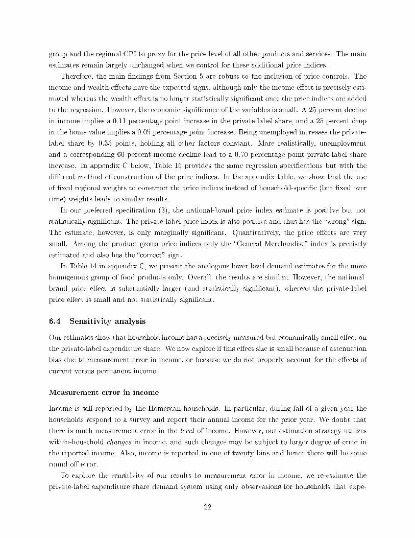
group and the regional CPI to proxy for the price level of all other products and services. The main

estimates remain largely unchanged when we control for these additional price indices.

Therefore, the main �ndings from Section 5 are robust to the inclusion of price controls. The

income and wealth e�ects have the expected signs, although only the income e�ect is precisely esti-

mated whereas the wealth e�ect is no longer statistically signi�cant once the price indices are added

to the regression. However, the economic signi�cance of the variables is small. A 25 percent decline

in income implies a 0.11 percentage point increase in the private-label share, and a 25 percent drop

in the home value implies a 0.05 percentage point increase. Being unemployed increases the private-

label share by 0.35 points, holding all other factors constant. More realistically, unemployment

and a corresponding 60 percent income decline lead to a 0.70 percentage point private-label share

increase. In appendix C below, Table 16 provides the same regression speci�cations but with the

di�erent method of construction of the price indices. In the appendix table, we show that the use

of �xed regional weights to construct the price indices instead of household-speci�c (but �xed over

time) weights leads to similar results.

In our preferred speci�cation (3), the national-brand price index estimate is positive but not

statistically signi�cant. The private-label price index is also positive and thus has the �wrong� sign.

The estimate, however, is only marginally signi�cant. Quantitatively, the price e�ects are very

small. Among the product group price indices only the �General Merchandise� index is precisely

estimated and also has the �correct� sign.

In Table 14 in appendix C, we present the analogous lower level demand estimates for the more

homogenous group of food products only. Overall, the results are similar. However, the national-

brand price e�ect is substantially larger (and statistically signi�cant), whereas the private-label

price e�ect is small and not statistically signi�cant.

6.4 Sensitivity analysis

Our estimates show that household income has a precisely measured but economically small e�ect on

the private-label expenditure share. We now explore if this e�ect size is small because of attenuation

bias due to measurement error in income, or because we do not properly account for the e�ects of

current versus permanent income.

Measurement error in income

Income is self-reported by the Homescan households. In particular, during fall of a given year the

households respond to a survey and report their annual income for the prior year. We doubt that

there is much measurement error in the level of income. However, our estimation strategy utilizes

within-household changes in income, and such changes may be subject to larger degree of error in

the reported income. Also, income is reported in one of twenty bins and hence there will be some

round-o� error.

To explore the sensitivity of our results to measurement error in income, we re-estimate the

private-label expenditure share demand system using only observations for households that expe-

22

rienced relatively large income changes in the sample period. In particular, we select households

who experienced at least one n percent income change in absolute value relative to the prior year.

Table 9 displays our preferred speci�cation of the AIDS private-label share system in column (1),

and compares the estimates to speci�cations for households who experienced an income change of at

least n =10 or n = 20 percent in absolute value in columns (2) and (3). The estimated income e�ect

decreases slightly (in absolute value) in speci�cation (2) and by a modest amount in speci�cation

(3), from -0.38 to -0.293. These results do not provide evidence for attenuation bias.

We also explore the extent of measurement error in income required to a�ect our conclusions

about the income e�ect on private-label demand signi�cantly. Let Iht be reported income, which

is a noisy measure of the true household income, I∗ht: log(Iht) = log(I∗ht) + ωht. The measurement

error in reported income, ωht, leads to attenuation bias in the estimated income e�ect:

plim δI =1

1 + σ2ω

σ2log(I∗)

δI . (6)

Here, σ2ω/σ2log(I∗) is the noise-to-signal ratio, the variance of the measurement error relative to the

variance of true income. We conduct the following thought experiment. Suppose we knew the

noise-to-signal ratio. Then we could infer the true income e�ect from the estimated, biased income

e�ect from equation (6), and correspondingly we could predict the true change in the private-label

expenditure share for di�erent changes in household income. In Table 11 we report the corresponding

true income e�ects based on estimated income e�ects and small (0.5), medium (1), and large (10)

values of the noise-to-signal ratio. For the �medium� degree of measurement error the true income

e�ects would be twice as large as the measured e�ects, but the economic signi�cance of the income

e�ect would still be small. Only for the unrealistically �large� degree of measurement error with a

noise-to-signal ratio of 10 would we �nd a substantially changed true income e�ect.

Current versus permanent income

Our identi�cation strategy relies year to year �within� household variation in income. This variation

in income can have both a permanent and a transient component. We might suspect that the within

variation is driven more by short term shocks to income and hence our causal estimates may re�ect

more of the response to changes in transient as opposed permant income. In this section, we explore

sensitivity of our income e�ect estimates to the distinction between permanent and current income.

Our estimated demand models contain a household-level unemployment indicator that may

proxy for expectations about future income and hence capture permanent income e�ects. To further

explore the di�erence between the e�ects of current and permanent income we introduce several

additional measures that may capture permanent income components in the private-label share

equation. The results are reported in Table 9. In column (4), we add an indicator for the year

when the household became unemployed in addition to the unemployment indicator. The �became

unemployed� estimate is small and not statistically di�erent from zero. Hence, the evidence does

23

not suggest that the e�ects of short term unemployment are di�erent from the e�ects of long term

unemployment. Older households may perceive income changes as more permanent than younger

households. Correspondingly, in column (5) we add the interaction of income with the log age of the

household head to the share equation. Also, unemployed households may perceive income changes

as more permanent, and hence we add an interaction of log income and the unemployment indicator

in column (6). Both estimated interactions are small and not statistically signi�cant.

In Table 10 we examine the e�ect of lagged (log) income on the private-label share. We compare

model speci�cations that include between one and four income lags. All four models with lags

indicate that both current and past income levels a�ect private-label demand. The �rst income lag

is mostly of equal or slightly larger magnitude than the contemporaneous income e�ect, whereas

the higher-order lags are smaller. In the speci�cation with four lags, the third lag is not statistically

di�erent than zero, but the fourth lag is statistically signi�cant. We can match prices to the

household-level purchases only for the years 2006-2011, and hence we cannot explore the e�ect of

lags of order �ve or higher. However, the declining coe�cient pattern in Table 10 suggests that

four lags are likely to capture most of the past income e�ects. Further support for this conjecture

is provided by the estimates for the upper level CPG expenditure model in Table 12, where we

�nd that only the �rst three lags of income have a statistically signi�cant impact on spending. The

lagged income results are consistent with a permanent income e�ect, whereby households form future

income expectations based on their contemporaneous and past income levels. The evidence is also

consistent with a partial adjustment view of private-label demand, whereby households change their

purchase habits only slowly. Such persistence in choice behavior has been extensively documented

in the brand choice literature (see Dube, Hitsch, and Rossi 2010 for an overview of the literature).

One possible explanation for the statistically signi�cant e�ect of the �rst income lag is mea-

surement error. As discussed previously, Nielsen collects the previous year's income in a survey

conducted at the end of the fall. If households erroneously report their current-year income, the

�rst lag of the income variable that is matched to the transaction data using the procedure explained

in Section 3.1 would correspond to the true contemporaneous income. The same logic, however,

cannot explain the statistically signi�cant higher-order income lags, and hence we conclude, once

again, that our results are unlikely to be a�ected by measurement error.

In summary, we do not �nd evidence that the income e�ect estimates are small because of attenua-

tion bias from measurement error. However, we �nd that private-label demand is a�ected by current

and past income levels, consistent with both a permanent income and a partial adjustment view.

Examining the magnitude of the income e�ects, we �nd that if we do not control for lagged income

the private-label share increases by 0.11 percentage points for a 25 percent income reduction. For

a permanent 25 percent income reduction the predicted share increase is 0.38 points, calculated

using the e�ects of both current income and the �rst four income lags. Hence, the e�ect from a

permanent income change is signi�cantly larger than the e�ect from a contemporaneous income

change. Nonetheless, in absolute terms the income e�ect is small. Real median household incomes

in the U.S. decreased by less than 10 percent in the years during and after the Great Recession

24

relative to the peak value in 2007.19 The corresponding predicted e�ect on the overall private-label

share is an increase of less than 0.14 points. Even for a large income change, for example if a house-

hold becomes unemployed and experiences a permanent 60 percent drop in income, the predicted

private-label share of 1.6 points is modest when compared to the overall private-label-share level.

6.5 Are private-label products inferior goods?

So far we have established that the private-label expenditure share is decreasing in household-

level income and housing wealth. However, this �nding does not directly imply that private-label

products are inferior goods. Both the demand for private-label products and national brands are

a�ected by income and wealth. Suppose that private-label and national-brand demand increases

in income and wealth, but that the demand for national brands increases at a faster rate than the

demand for private-label products. The private-label share is then decreasing in income and wealth,

even though private-label products are normal goods.

The Marshallian demand for private-label products corresponding to the model in Section 6.1

is given by

QPL = syCPGPPL

. (7)

Again, to simplify the notation, we have omitted household and time subscripts. The income

elasticity of private-label demand is therefore

ePL =∂ log(QPL)

∂ log(I)=∂ log(s)

∂ log(I)+∂ log(yCPG)

∂ log(I)

=γIs

+ δI (8)

The income elasticity of private-label demand depends on the income elasticity of the private-label

expenditure share and the income elasticity of total CPG expenditure. The household wealth elas-

ticity is derived analogously. Based on our �ndings above in Section 6.4 we also incorporate lagged

(log) income levels in the upper and lower level demand equations. Generalizing the income elastic-

ity formula (8) to this case is straightforward. Let δI,−l and γI,−l be the parameters corresponding

to the lth income lag in upper and lower level demand. The elasticity of private-label demand with

respect to a permanent income change is then given by

ePL =1

s

L∑l=0

γI,−l +L∑l=0

δI,−l. (9)

To estimate the income elasticity (8) we �t the upper level CPG expenditure model (3). The

19US. Bureau of the Census, Real Median Household Income in the United States [MEHOINUSA672N], retrievedfrom FRED, Federal Reserve Bank of St. Louis https://research.stlouisfed.org/fred2/series/MEHOINUSA672N/,April 25, 2015.

25

corresponding results are reported in Table 12.20 We use the same price level controls that we used

in the lower level AIDS share regression, and in column (3) we also include recession and post-

recession indicators and the trend variables. In column (4) we add the �rst four lags of log income

to the expenditure equation. The estimates of the �rst three lags are all statistically signi�cant,

while the fourth lag is not statistically di�erent from zero. Also, the e�ect of the �rst income lag

on CPG spending is larger than the contemporaneous e�ect. The e�ect sizes are declining for the

lags of order l > 1. Based on the model including all lags (4), the estimated income elasticity of

CPG expenditure with respect to contemporaneous income is 0.025. This income e�ect is small

but precisely estimated. The elasticity with respect to a permanent income change is substantially

larger, 0.124. The estimated wealth e�ect is smaller and not statistically di�erent from zero.

In Table 13 we report the predicted income and wealth elasticities of demand. The predicted

elasticities of the private-label expenditure share are evaluated at the median private-label share

across households (see equation 8). We �nd that the point estimate of the income elasticity of

private-label demand is positive both for contemporaneous and permanent income changes, indi-

cating that the private-label product group is a normal good. However, a 95 percent con�dence

interval includes a range of negative and positive values. Hence, despite the positive point estimates

we cannot be sure if the private-label product group is an inferior or normal good. The economic

signi�cance of the income elasticity estimates is small. For instance, a 10 percent permanent increase

in income would increase private-label demand by about 0.53 percent, while the corresponding con-

temporaneous income e�ect on private-label demand is only about 0.04 percent. The estimated

wealth elasticity is also small and not statistically di�erent from zero.

7 Sources of private-label-share growth

A key �nding of our analysis (see, for example, the trend coe�cient in Table 8) is the strong positive

trend in the private-label share of 0.44 percentage points per year. The trend appears to be the

main source of private-label growth over our sample period, whereas the e�ects of income and wealth

shocks were comparatively small. In this section, we investigate the role of product quality and new

private-label product introductions as possibles sources of this trend.

Private-label product quality

We investigate whether the upward trend in the private-label share was uniform or concentrated in

speci�c private-label quality tiers. Some articles in the trade press suggest that the private-label-

share growth re�ects the increasing availability of high-quality private-label products (PR Newswire

2011). Describing the increasing availability of high-quality private-label products, Kumar and

Steenkamp 2007 argue that �it is almost as if quality has now become a commodity.� They note

that several leading US retail chains have produced private-label alternatives that are now higher-

20Table 19 provides estimates of the upper level demand equation using price indices with �xed region weights.Table 15 provides the results for only food products.

26

rated than their national-brand counterparts in Consumer Reports. According to Sarah Theodore,

a beverage analyst at Mintel International: �Private label has really been gaining ground for several

years now because retailers have put a lot more emphasis on quality. They've really created brands

that can stand up to national brands, and that's something that's been going on for quite a while

now. The recession has kind of accelerated this trend a little bit, and in some categories more than

others. But it was a movement that was taking place long before the economy fell apart� (Rouan

2010).

Either due to demand-side or supply-side factors, the private-label share increase could be due to

increased spending on high-quality private-label products that are similar to national brands along

their actual or perceived attributes. Unfortunately, we do not have a direct measure of product

quality as there is no consistent source measuring private-label quality during our sample period.21

Also, the data available from the Kilts Center of Marketing do not include information on the

name of private-label products and hence we cannot infer a quality tier (for example standard or

premium) from the brand name.22 Instead, we de�ne an indirect measure of quality based on the

relative private-label/national-brand product price. Our analysis will therefore explore whether

the trend in overall private-label shares appears to be associated with a trend towards purchasing

private labels with prices comparable to those of the national-brand counterparts. Such a de�nition

is meaningful if the relative price of a private-label product is positively correlated with its quality.

Although plausible, we cannot test this assumption.

We calculate the relative private-label/national-brand prices using the transaction prices from

the Homescan data, not the o�ered prices from the RMS data. This allows us to classify and analyze

all private-label products in our data, not just those sold by the retailers observed in the RMS data.

To classify the private-label products into di�erent quality tiers we use the following approach.

(i) We focus on product groups that are in the same category and have volumes that are measured

in the same equivalent units, such as ounces or pounds. This allows us to express prices in

equivalent units that can be compared across di�erent products.

(ii) We calculate the median monthly price (in equivalent units) of each product based on the

observed transaction prices in the Homescan data.

(iii) For the national-brand products, we calculate the monthly product-group median across all

product prices calculated in (ii).

(iv) Even at the monthly level there are often few or no price observations for a given product.

Hence, for each private-label product and month t we calculate the median of the prices in (ii)

over all periods t− 11, . . . , t. We also calculate an analogous moving average for the national-

21Apelbaum, Gerstner, and Naik 2003 use data collected from Consumer Reports. However, for our sample periodConsumer Reports did not systematically provide a consistent measure of private-label versus national-brand qualityacross CPG categories. Conducting a survey of retailers, as in Hoch and Banerji 1993, is beyond the scope of thispaper.

22The brand description for all private-label products is �CTL BR� (control brand) in the Kilts Center data.

27

brand product group prices in (iii). The relative price of a private-label product is then given

by the ratio of the private-label and national-brand product group moving averages.

We repeatedly use medians, not (weighted) averages in this approach because the observations for

any given product are sparse and because we would like to minimize the resulting in�uence of

outliers on our results.

Based on these relative prices, we classify the private-label products into di�erent quality tiers

based on the thresholds 0.6, 0.7, 0.8, 0.9, and 1. The tier of private-label products with the

lowest quality are those with relative price rjt < 0.6. The second lowest quality tier is de�ned as

0.6 ≤ rjt < 0.7, etc. We correspondingly obtain six quality tiers.23 By design, this approach allows

product j to be in di�erent quality tiers across time if its relative price changes signi�cantly.

In Figure 7, we show the evolution of the private-label share during 2004-2011 in each quality

tier. In each tier the average share (across months) increased from 2004 to 2011. The largest

increases were in the > 100% tier (0.82 points) and in the 70 − 80% tier (0.70 points), although,

as a percentage of the base share, the increase was somewhat larger in the 70 − 80% tier than in

the > 100% tier. The smallest increases were in the 90− 100% tier (0.15 points) and in the ≤ 60%

group (0.19 points); the latter increase was the smallest as a percentage of the base share. Overall,

it does not appear that there was a strong, systematic relationship between the private-label-share

growth and the quality level of the products.

New product introductions

The positive trend in the private-label share may re�ect new product introductions by the retailers.

In a recent report, IRI describes private-label products as alternatives that �bring something new

to the market... new products, new attributes, new sizes... private labels are opening doors to

attributes which have historically been out of the reach of many consumers by bringing them into

an a�ordable price range.�24

In Figure 8, we show the number of new products introduced in each month from 2006 to 2011,

separately for private-label and national-brand products. We classify a product as �new� if there is

no purchase record for the product in the Homescan data in 2004 or 2005, and we exclude UPC's that

appear in the data for less than four months to distinguish between true product introductions and

promotional UPC's. The number of new product introductions per month is substantial, and the

number of national-brand product introductions is larger than the number of private-label product

introductions. The count of new products may be misleading, however, because we equate products

with UPC's, and hence any slight modi�cation of an existing product counts as a new product.

Alternatively, in Figure 9, we display the private-label and national-brand new-product-expenditure

shares. Here, we classify a product as �new� in a given month if it was either introduced within the

23The results of the analysis were robust when we experimented with di�erent thresholds to de�ne the quality tiers.

24The report is available online at:http://www.symphonyiri.com/Insights/Publications/TimesTrends/tabid/106/Default.aspx.

28

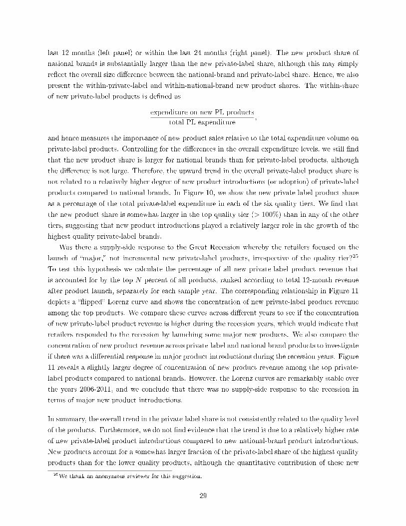
last 12 months (left panel) or within the last 24 months (right panel). The new product share of

national brands is substantially larger than the new private-label share, although this may simply

re�ect the overall size di�erence between the national-brand and private-label share. Hence, we also

present the within-private-label and within-national-brand new product shares. The within-share

of new private-label products is de�ned as

expenditure on new PL products

total PL expenditure,

and hence measures the importance of new product sales relative to the total expenditure volume on

private-label products. Controlling for the di�erences in the overall expenditure levels, we still �nd

that the new product share is larger for national brands than for private-label products, although

the di�erence is not large. Therefore, the upward trend in the overall private-label product share is

not related to a relatively higher degree of new product introductions (or adoption) of private-label

products compared to national brands. In Figure 10, we show the new private-label product share

as a percentage of the total private-label expenditure in each of the six quality tiers. We �nd that

the new product share is somewhat larger in the top quality tier (> 100%) than in any of the other

tiers, suggesting that new product introductions played a relatively larger role in the growth of the

highest quality private-label brands.

Was there a supply-side response to the Great Recession whereby the retailers focused on the

launch of �major,� not incremental new private-label products, irrespective of the quality tier?25

To test this hypothesis we calculate the percentage of all new private-label product revenue that

is accounted for by the top N percent of all products, ranked according to total 12-month revenue

after product launch, separately for each sample year. The corresponding relationship in Figure 11

depicts a ��ipped� Lorenz curve and shows the concentration of new private-label product revenue

among the top products. We compare these curves across di�erent years to see if the concentration

of new private-label product revenue is higher during the recession years, which would indicate that

retailers responded to the recession by launching some major new products. We also compare the

concentration of new product revenue across private-label and national brand products to investigate

if there was a di�erential response in major product introductions during the recession years. Figure

11 reveals a slightly larger degree of concentration of new product revenue among the top private-

label products compared to national brands. However, the Lorenz curves are remarkably stable over

the years 2006-2011, and we conclude that there was no supply-side response to the recession in

terms of major new product introductions.

In summary, the overall trend in the private-label share is not consistently related to the quality level

of the products. Furthermore, we do not �nd evidence that the trend is due to a relatively higher rate

of new private-label product introductions compared to new national-brand product introductions.

New products account for a somewhat larger fraction of the private-label share of the highest quality

products than for the lower quality products, although the quantitative contribution of these new

25We thank an anonymous reviewer for this suggestion.

29

high-quality products to the overall trend is small.

8 Conclusions

This paper provides clear evidence for a negative causal e�ect of income on the private-label share

in CPG expenditures, whereas the estimated wealth e�ect is also negative but not statistically

di�erent from zero. The elasticity of demand for the private-label product group with respect to

income is small and positive, but a 95 percent con�dence interval contains both positive and negative

values. Previous work on the relationship between income and private-label shares has either relied

on cross-sectional or aggregate time series analyses. Our approach to estimating causal e�ects of

income exploits within-household variation in income controlling for selection or cohort e�ects which

a�ict cross-sectional analyses. The Great Recession provides the key source of income and wealth

variation in our data. In particular, the e�ect of the Great Recession on economic conditions was

large and there were large di�erences in the impact of the recession across regions and households,

a fact we use to justify that within-household income and wealth changes are as good as randomly

assigned conditional on other controls.

The estimates of the causal e�ect of income are small and smaller than those obtained using

the cross-sectional variation in our panel data. Selection could be at the root of the di�erence

between results obtained from the cross-sectional versus within-household variation in the data.

That is, there is an unobservable characteristic of households which is correlated with income and

the demand for private-label versus national-brand products. It is also possible that there are

cohort e�ects which mask the true causal relationship between income and private-label demand.

For example, suppose older consumers have a di�erent perception of quality di�erences between

national-brand and private-label products than younger cohorts as well as higher income and wealth.

Then in the cross-section, these cohort e�ects could induce a correlation between income and private-

label demand. While we feel con�dent that we can identify the causal impact of income from our

household panel data, we do not identify the unobservable factors which may lead to a spuriously

high level of correlation between income and private-label demand. Clearly, understanding these

unobservables should be one of the goals of the private-label research agenda.

To interpret the estimated income and wealth e�ects as direct demand e�ects, we also need

to condition on local market conditions, in particular prices, that may be correlated with within-

household changes in income and wealth. Hence we construct local national-brand and private-label

price indices that are customized to each household's spending patterns. Conditional on these price

controls, we can interpret the income and wealth e�ects on private-label demand as valid direct

demand e�ects as de�ned in the microeconomic theory of the consumer.

The estimated income e�ects are precisely measured but small. A sensitivity analysis shows

that the small e�ect size is unlikely to be the result of attenuation bias due to measurement error.

We also extend the analysis beyond a contemporaneous relationship between income and private-

label shares and also add lagged income levels to our speci�cation. We �nd signi�cant lagged

30

relationships. This evidence is consistent with a permanent income explanation, but also with a

form of partial adjustment whereby purchase patterns change only slowly.

The small economic signi�cance of the income estimates is in stark contrast to some prior work

in marketing research, and at odds with many views voiced in the industry at the time of the Great

Recession. The di�erences between our �ndings and the results in some prior studies (e.g. Lamey,

Deleersnyder, Dekimpe, and Steenkamp 2007) can be explained in a variety of ways. First, we

have di�erent data sources with a much larger number of products and a di�erent (more recent)

time span. Second, our identi�cation strategy relies on di�erences across households in the within-

household variation in income and wealth that, as we argued, is plausibly exogenous or �as good

as randomly assigned� conditional on supply-side controls. Such an analysis is feasible even when

controlling for a �exible overall trend or time-speci�c e�ects. An analysis using aggregate time

series data as the basis for causal inference is based on the assumption that the counterfactual

private-label demand outcome in the absence of aggregate income changes during a recession can be

predicted or extrapolated using a trend based on pre-recession data. This is a di�erent identi�cation

strategy and one can debate which set of assumptions is more or less plausible for the purpose of

causal inference.

We also document the supply response of national brand and private labels to the Great Re-

cession. Contrary to the views expressed in the industry press, we do not �nd that national-brand

manufacturers reduced the e�ective price of national-brand products relative to private-label prod-

ucts.

Our estimates reveal a large trend in the private-label share that predates the years of the Great

Recession. The trend does not stem systematically from speci�c private-label quality tiers, although

we can only imperfectly proxy for product quality using relative private-label versus national-brand

price ratios. The trend also appears to be unrelated to the overall rate of private-label versus

national-brand product introductions. According to our analysis, the overall trend represents a

greater threat to national-brand products than economic downturns. Therefore, an important task

for future private-label research is to uncover the origins of the trend before any meaningful conclu-

sions can be made as to what �rm policies might alter this trend.

31

References

Ailawadi, K. L., S. A. Neslin, and K. Gedenk (2001): �Pursing the Value-Conscious Consumer:

Store Brands versus National Brand Promotions,� Journal of Marketing, 65(1), 71�89.

Ailawadi, K. L., K. Pauwels, and J. B. Steenkamp (2008): �Private-Label Use and Store

Loyalty,� Journal of Marketing, 72, 19�30.

Ang, S.-H., S. M. Leong, and P. Kotler (2000): �The Asian Apocalypse: Crisis Marketing for

Consumers and Businesses,� Long Range Planning, 33, 97�119.

Apelbaum, E., E. Gerstner, and P. Naik (2003): �The E�ects of Expert Quality Evaluations

Vs. Brand,� Journal of Product and Brand Management, 12(3), 154�165.

Batra, R., and I. Sinha (2000): �Consumer-Level Factors Moderating the Success of Private

Label Brands,� Journal of Retailing, 76(2), 175�191.

Bronnenberg, B. J., J. Dube, M. Gentzkow, and J. M. Shapiro (2014): �Do Pharmacists

Buy Bayer? Informed Shoppers and the Brand Premium,� Discussion Paper 20295, National

Bureau of Economic Research.

Cha, W., P. Chintagunta, and S. Dhar (2015): �Food Purchases during the Great Recession,�

manuscript, University of Chicago Booth School of Business.

Deaton, A., and J. Muellbauer (1980a): �An Almost Ideal Demand System,� American Eco-

nomic Review, 70(3), 312�326.

(1980b): Economics and Consumer Behavior. Cambridge University Press.

Dhar, S. K., and S. J. Hoch (1997): �Why Store Brand Penetration Varies by Retailer,� Mar-

keting Science, 16(3), 2208�227.

Dube, J., G. Hitsch, and P. E. Rossi (2010): �State Dependence and Alternative Explanations

for Consumer Inertia,� RAND Journal of Economics, 41(3), 417�445.

Erdem, T., Y. Zhao, and A. Valenzuela (2004): �Performance of Store Brands: a cross-

country analysis of consumer store-brand preferences, perceptions and risk,� Journal of Marketing

Research, XLI, 86�100.

Estelami, H., D. R. Lehmann, and A. C. Holden (2001): �Macro-economic determinants of

consumer price knowledge: A meta-analysis of four decades of research,� International Journal

of Research in Marketing, 18, 341�355.

Frank, J. N. (2010): �Consumers Plan to Stick with Private Label; Price Remains the Reason,�

Private Label Buyer, 25, 6.

32

Gicheva, D., J. Hastings, and S. Villas-Boas (2010): �Investigating Income E�ects in Scan-

ner Data: Do Gasoline Prices A�ect Grocery Purchases? Investigating Income E�ects in Scanner

Data: Do Gasoline Prices A�ect Grocery Purchases? Investigating Income E�ects in Scanner

Data: Do Gasoline Prices A�ect Grocery Purchases?,� American Economic Review: Papers Pro-

ceedings, 100, 480�484.

Gordon, B. R., A. Goldfarb, and Y. Li (2013): �Does Price Elasticity Vary with Economic

Growth? A Cross-Category Analysis,� Journal of Marketing Research, 50(1), 4�23.

Guerrieri, V., D. Hartley, and E. Hurst (2013): �Endogenous Gentri�cation and Housing

Price Dynamics,� Journal of Public Economics, 100, 45�60.

Hammerbeck, P. (2008): �Store Brands: Ignore Them at Your Peril,� Brand Packaging.

Hansen, K., V. Singh, and P. Chintagunta (2006): �Understanding Store-Brand Purchase

Behavior Across Categories,� Marketing Science, 25(1), 75�90.

Hausman, J., G. Leonard, and J. D. Zona (1994): �Competitive Analysis with Di�erentiated

Products,� Annales d'Économie et de Statistique, 34, 159�180.

Hoch, S. J., and S. Banerji (1993): �When Do Private Labels Succeed?,� Sloan Management

Review, 34(4), 57�67.

Iacoviello, M. (2011): �Housing Wealth and Consumption,� International Finance Discussion

Papers 1027, Board of Governors of the Federal Reserve System.

Imbens, G. W., and D. R. Rubin (2015): Causal Inference for Statistics, Social, and Biomedical

Sciences: An Introduction. Cambridge University Press.

Kamakura, W. A., and R. Y. Du (2012): �How Economic Contractions and Expansions A�ect

Expenditure Patterns,� Journal of Consumer Research, 39, 229�247.

Kilts Center for Marketing (2013): �Consumer Panel Dataset Manual,� Discussion paper,

Booth School of Business, University of Chicago.

Kim, J., G. M. Allenby, and P. E. Rossi (2002): �Modeling Consumer Demand for Variety,�

Marketing Science, 21(3), 229�250.

Kumar, N., and J.-B. E. M. Steenkamp (2007): Private Label Strategy: How to Meet the Store

Brand Challenge. Harvard Business Review Press.

Lamey, L., B. Deleersnyder, M. G. Dekimpe, and J. B. Steenkamp (2012): �The E�ect of

Business-Cycle Fluctuations on Private-Label Share: What Has Marketing Conduct Got to Do

With It?,� Journal of Marketing, 76, 1�19.

33

Lamey, L., B. Deleersnyder, M. G. Dekimpe, and J.-B. E. Steenkamp (2007): �How Busi-

ness Cycles Contribute to Private-Label Success: Evidence from the United States and Europe,�

Journal of Marketing, 71(1), 1�15.

Ma, Y., K. L. Ailawadi, D. K. Gauri, and D. Grewal (2011): �An Empirical Investigation

of the Impact of Gasoline Prices on Grocery Shopping Behavior,� Journal of Marketing, 75(2),

18�35.

Mian, A., K. Rao, and A. Sufi (2013): �Household Balance Sheets, Consumption, and the

Economic Slump,� Quarterly Journal of Economics, 128(4), 1687�1726.

Mian, A., and A. Sufi (2014): �What Explains the 2007-2009 Drop in Employment?,� Economet-

rica, 82(6), 2197�2223.

Mian, A., A. Sufi, and F. Trebbi (2015): �Foreclosures, House Prices, and the Real Economy,�

Journal of Finance, 70(6), 2587�2634.

Murphy, P. E., and G. R. Laczniak (1979): �Generic Supermarket Items: A Product and

Consumer Analysis,� Journal of Retailing, 55(2), 3�14.

Nevo, A., and A. Wong (2015): �The Elasticity of Substitution Between Time and Market Goods:

Evidence from the Great Recession,� Working Paper.

Nielsen (2011): �Private Brand U.S. Outlook,� Discussion paper, The Nielsen Company.

PR Newswire (2011): �Private Label Gets a Quality Reputation, Causing Consumers to Change

Their Buying Habits,� PR Newswire, January 20.

Quelch, J. A., and D. Harding (1996): �Brands Versus Private Labels: �ghting to win,� Harvard

Business Review, 1, 99�109.

Raju, J. S., R. Seethuraman, and S. K. Dhar (1995): �The Introduction and Performance of

Store Brands,� Management Science, 41, 957�978.

Rosen, D. L. (1984): �Consumer Perceptions of Quality for Generic Grocery Products: A Com-

parison across product Categories,� Journal of Retailing, 60, 64�80.

Rouan, R. (2010): �A new label on quality,� Beverage Industry, 101.9, 22�23.

Stroebel, J., and J. Vavra (2016): �House Prices, Local Demand, and Retail Prices,� NBER

Working Paper 20710.

ter Braak, A., I. Geyskens, and M. G. Dekimpe (2014): �Taking Private Labels Upmarket:

Empirical Generalizations on Category Drivers of Premium Private Label Introductions,� Journal

of Retailing, 90(2), 125�140.

34

van Heerde, H. J., M. J. Gijsenberg, M. G. Dekimpe, and J.-B. E. Steenkamp (2013):

�Price and Advertising E�ectiveness over the Business Cycle,� Journal of Marketing Research,

50(2), 177�193.

Wong, E. (2008): �Will Private Label Clean Up Now?,� Brandweek, 49, S40�42.

35

Table 1: Homescan Sample Size

Year Households Trips

(mm)

Transactions

(mm)

Expenditures

($mm)

2004 Raw 39,577 5.7 38.7 129.2

Filtered 31,878 4.6 30.7 100.8

Income-Matched 27,977 3.5 22.9 75.3

2005 Raw 38,862 5.5 38.4 131.3

Filtered 32,918 4.8 32.2 108.9

Income-Matched 29,496 3.7 24.6 83.0

2006 Raw 37,783 5.2 36.0 127.4

Filtered 31,866 4.5 30.7 107.9

Income-Matched 28,419 3.6 23.8 83.1

2007 Raw 63,345 8.2 60.2 222.9

Filtered 53,319 7.2 51.7 190.8

Income-Matched 42,892 5.3 36.5 134.4

2008 Raw 61,437 7.9 57.6 223.7

Filtered 52,204 7.0 49.8 193.3

Income-Matched 41,300 5.1 35.4 137.2

2009 Raw 60,502 7.7 56.3 222.7

Filtered 52,134 6.9 49.3 195.0

Income-Matched 40,469 5.1 34.8 137.6

2010 Raw 60,654 7.7 55.1 222.3

Filtered 53,371 7.0 48.5 192.2

Income-Matched 42,511 5.1 34.9 138.4

2011 Raw 62,085 8.0 56.9 236.1

Filtered 55,526 7.4 50.5 206.9

Income-Matched

2012 Raw 60,534 7.5 53.8 230.2

Filtered 52,786 6.8 46.6 195.1

Income-Matched

Note: The �ltering procedure is described in Section 3.1. The rows indicated as �Income-Matched�summarize all observations in household years t that can be matched to the income that is reported in theyear t+ 2 data (see Section 3.1). Correspondingly, there are no such matched observations in the last twosample years, 2011 and 2012.

36

Table 2: Comparison of the Distribution of Demographics: Census CPS vs. Homescan

Census-CPS Homescan

Age

<5 6 2

5-17 18 13

18-24 10 6

25-44 27 17

45-64 26 41

65+ 13 19

Education

< HS 14 4

HS 31 25

Some College 28 30

College 18 30

Graduate 9 12

Income

10th Pctl $ 11,904 $ 17,500

20th Pctl $ 20,000 $ 27,500

50th Pctl $ 49,445 $ 55,000

80th Pctl $100,065 $ 85,000

90th Pctl $138,923 $112,500

Table 3: Private-Label Shares Across Household-Years

Statistic PL SharePL Share:

Food Only

Mean 19.50 20.66

St. Dev. 10.76 11.86

1st Pctl. 8.05 7.99

5th Pctl. 9.09 9.15

25th Pctl. 13.79 14.39

Median 19.18 20.37

75th Pctl. 26.41 28.33

95th Pctl. 73.12 74.08

99th Pctl. 94.62 94.75

Percent Share = 0 0.09 0.20

N. Obs. 416,001 415,968

Note: The data are pooled over all household-years. The reported statistics are weighted using the projectionfactors. We normalize the projection factors to sum to one within each year.

37

Table 4: Pre-Trend Analysis

Pre-recession Recession Estimate t-value Pr{> |t|} No. obs.

All Products

Private-Label Share/Unemployment

2004/2006 2007/2009 -0.042 -1.974 0.049 2,185

2005/2006 2007/2009 -0.007 -0.331 0.741 2,183

Q1 2004/Q1 2007 Q2 2007/Q2 2009 -0.027 -1.267 0.205 2,147

Q1 2005/Q1 2007 Q2 2007/Q2 2009 0.018 0.861 0.389 2,195

Q1 2006/Q1 2007 Q2 2007/Q2 2009 -0.012 -0.562 0.574 2,199

Private-Label Share/Log Zillow Index

2004/2006 2007/2009 0.001 0.109 0.913 5,985

2005/2006 2007/2009 -0.028 -2.135 0.033 5,934

Q1 2004/Q1 2007 Q2 2007/Q2 2009 -0.001 -0.068 0.946 5,793

Q1 2005/Q1 2007 Q2 2007/Q2 2009 -0.027 -2.051 0.040 5,985

Q1 2006/Q1 2007 Q2 2007/Q2 2009 -0.022 -1.720 0.086 6,067

Private-Label Share/Log Income

2004/2006 2007/2009 0.007 0.795 0.427 13,931

2005/2006 2007/2009 0.003 0.327 0.744 15,797

Q1 2004/Q1 2007 Q2 2007/Q2 2009 0.000 -0.058 0.954 13,931

Q1 2005/Q1 2007 Q2 2007/Q2 2009 0.000 -0.035 0.972 15,794

Q1 2006/Q1 2007 Q2 2007/Q2 2009 -0.003 -0.336 0.737 17,179

Food

Private-Label Share/Unemployment

2004/2006 2007/2009 -0.037 -1.711 0.087 2,180

2005/2006 2007/2009 -0.002 -0.092 0.927 2,182

Q1 2004/Q1 2007 Q2 2007/Q2 2009 -0.009 -0.438 0.662 2,145

Q1 2005/Q1 2007 Q2 2007/Q2 2009 0.030 1.406 0.160 2,194

Q1 2006/Q1 2007 Q2 2007/Q2 2009 -0.006 -0.290 0.772 2,198

Private-Label Share/Log Zillow Index

2004/2006 2007/2009 -0.006 -0.472 0.637 5,970

2005/2006 2007/2009 -0.026 -1.995 0.046 5,932

Q1 2004/Q1 2007 Q2 2007/Q2 2009 -0.003 -0.233 0.815 5,791

Q1 2005/Q1 2007 Q2 2007/Q2 2009 -0.019 -1.502 0.133 5,984

Q1 2006/Q1 2007 Q2 2007/Q2 2009 -0.020 -1.573 0.116 6,066

Private-Label Share/Log Income

2004/2006 2007/2009 0.001 0.154 0.877 13,931

2005/2006 2007/2009 0.009 1.095 0.273 15,797

Q1 2004/Q1 2007 Q2 2007/Q2 2009 -0.011 -1.243 0.214 13,931

Q1 2005/Q1 2007 Q2 2007/Q2 2009 0.003 0.333 0.739 15,794

Q1 2006/Q1 2007 Q2 2007/Q2 2009 -0.004 -0.584 0.559 17,179

Note: This table reports the estimated correlation coe�cients between the change in the private-label share in thepre-recession period and the change in unemployment, the log Zillow index, and log income during the recessionperiod. The results are reported for di�erent time period de�nitions over which the changes are calculated. Forexample, �2004/2006� indicates the di�erence between the average of the variable in 2004 and 2006. �Q2 2007/Q22009� indicates the di�erence between the average of the variable in the second quarter of 2007 and the second quarterof 2009.

38

Table 5: Private-Label-Share Regression

pooled between

+ demog

Within withing

+

recession

within +

recession

+ trend

log(Income) -2.55 -2.93 -0.479 -0.345 -0.412

(0.0967) (0.18) (0.0669) (0.0654) (0.0654)

log(Wealth) -1.35 -1.23 -2.38 -0.01 -0.545

(0.146) (0.173) (0.119) (0.129) (0.141)

I{Unemployed} 0.00438 -0.314 0.268 0.358 0.373

(0.13) (0.213) (0.0837) (0.0814) (0.0812)

High School 0.342 0.695

(0.273) (0.29)

Some College 0.228 0.394

(0.144) (0.154)

College 0.718 0.612

(0.134) (0.149)

Post Graduate 0.503 0.711

(0.169) (0.156)

log(Age) 3.32 2.79

(0.264) (0.271)

No. Adults 0.16 0.368

(0.0712) (0.101)

No. Children 1.12 1.21

(0.0694) (0.103)

Female Hh. Head -2.86 -2.97

(0.172) (0.169)

Black -1.11 -1.17

(0.197) (0.21)

Asian -1.69 -1.58

(0.279) (0.271)

Hispanic -0.0924 -0.0665

(0.233) (0.23)

Divorced/Separated 0.686 0.608

(0.178) (0.153)

Widowed 0.902 0.806

(0.241) (0.222)

Single Hh. Head 0.293 0.233

(0.14) (0.139)

Mobile Home/Trailer 1.01 1.34

(0.301) (0.298)

Trend 0.0372

(0.00159)

I{Recession} 1.59 0.322

(0.0396) (0.0427)

39

Table 5: Private-Label-Share Regression

pooled between

+ demog

Within withing

+

recession

within +

recession

+ trend

I{Post Recession} 1.99 0.479

(0.0527) (0.0769)

Trend× I{Recession} 0.019

(0.00419)

Trend× I{Post Rec.} -0.029

(0.0039)

Fixed E�ects No No Hh. Hh. Hh.

No. Obs. 1,716,936 39,856 1,716,947 1,716,947 1,716,947

No. Missing 3,185,586 0 3,185,575 3,185,575 3,185,575

No. Clusters 39,413 195 39,413 39,413 39,413

R2 0.0723 0.122 0.567 0.569 0.57

40

Table 6: National-Brand/Private-Label Price Indices by Year

Year Mean NB/PL PriceRatio

2006 1.00002007 1.00132008 1.00622009 1.02012010 1.02002011 1.0186

Table 7: National-Brand/Private-Label Price Ratios and Local Economic Factors

∆ log(PNB/PPL) Regional ∆ log(PNB/PPL) Household(1) (2) (3) (4)

Constant 0.0028∗∗ 0.0126∗∗ 0.0026∗∗ 0.0131∗∗(0.0001) (0.0001) (0.0001) (0.0002)

2008 0.0022∗∗ 0.0085∗∗ 0.0021∗∗ 0.0089∗∗(0.0001) (0.0001) (0.0002) (0.0002)

2009 0.0083∗∗ 0.0036∗∗ 0.0072∗∗ 0.0022∗∗(0.0001) (0.0001) (0.0003) (0.0003)

2010 −0.0042∗∗ −0.0162∗∗ −0.0050∗∗ −0.0178∗∗(0.0001) (0.0002) (0.0001) (0.0003)

∆ log(Zillow) −0.0024∗∗ −0.0013∗∗ −0.0032∗∗ −0.0020∗∗(0.0003) (0.0003) (0.0005) (0.0005)

∆Unemployment 0.0009∗∗ 0.0006∗∗ 0.0011∗∗ 0.0008∗∗(0.00004) (0.00003) (0.0001) (0.0001)

∆ log(HH Real Income) −0.0002∗ −0.0002∗ −0.0002 −0.0002(0.0001) (0.0001) (0.0002) (0.0002)

∆ log(P ) Regional −0.3273∗∗ −0.3503∗∗(0.0036) (0.0071)

No. obs. 130,539 130,539 130,539 130,539R2 0.3919 0.4267 0.1468 0.1611

Note: ∗p < 0.05, ∗∗p < 0.01 corresponding to a two-tailed test.

41

Table 8: Lower Level Demand: AIDS Private-Label-Share System

within +

recession

+ trend

CPG

prices

CPG

prices +

proxies

log(Income) -0.412 -0.377 -0.38

(0.0654) (0.0718) (0.0713)

log(Wealth) -0.545 -0.149 -0.16

(0.141) (0.164) (0.164)

I{Unemployed} 0.373 0.34 0.353

(0.0812) (0.0905) (0.0906)

Trend 0.0372 0.0351 0.0368

(0.00159) (0.00402) (0.00456)

I{Recession} 0.322 0.175 0.138

(0.0427) (0.0453) (0.0489)

I{Post Recession} 0.479 0.296 0.24

(0.0769) (0.108) (0.111)

Trend× I{Recession} 0.019 0.0107 0.011

(0.00419) (0.00589) (0.00655)

Trend× I{Post Rec.} -0.029 -0.0229 -0.0295

(0.0039) (0.0054) (0.00578)

log(PI National Brand) 1.38 2.69

(5.84) (5.65)

log(PI Private Label) 2.92 2.64

(1.36) (1.35)

log(PI All CPG) 1.82 0.843

(6.15) (5.94)

log(CPI) 0.511

(1.01)

log(PI Gen. Merchandise) -2.21

(0.667)

Fixed E�ects Hh. Hh. Hh.

No. Obs. 1,716,947 1,335,207 1,317,596

No. Missing 3,185,575 3,567,315 3,584,926

No. Clusters 39,413 36,022 35,973

R2 0.57 0.576 0.578

42

Table 9: Sensitivity Analysis: AIDS Private-Label-Share System

(1) (2) (3) (4) (5) (6)

log(Income) -0.38 -0.329 -0.293 -0.38 -0.28 -0.374

(0.0713) (0.0776) (0.0807) (0.0713) (1.3) (0.0734)

log(Wealth) -0.16 -0.216 -0.08 -0.16 -0.155 -0.159

(0.164) (0.201) (0.216) (0.164) (0.164) (0.164)

I{Unemployed} 0.353 0.424 0.446 0.332 0.342 0.681

(0.0906) (0.107) (0.123) (0.112) (0.0906) (1.29)

I{Became Unemployed} 0.0353

(0.0939)

log(Income)×I{Unemployed} -0.0308

(0.119)

log(Age) -0.921

(3.43)

log(Income)×log(Age) -0.0244

(0.318)

Trend 0.0368 0.034 0.0405 0.0367 0.0382 0.0368

(0.00456) (0.00532) (0.00624) (0.00455) (0.0046) (0.00456)

I{Recession} 0.138 0.123 0.0988 0.139 0.151 0.138

(0.0489) (0.0579) (0.0685) (0.0491) (0.0493) (0.0489)

I{Post Recession} 0.24 0.396 0.206 0.243 0.255 0.241

(0.111) (0.161) (0.15) (0.111) (0.111) (0.111)

Trend× I{Recession} 0.011 0.0216 0.0125 0.0111 0.0112 0.011

(0.00655) (0.00906) (0.00904) (0.00655) (0.00655) (0.00655)

Trend× I{Post Rec.} -0.0295 -0.0308 -0.041 -0.0293 -0.0293 -0.0295

(0.00578) (0.00689) (0.00798) (0.00578) (0.00578) (0.00578)

log(PI National Brand) 2.69 1.16 1.04 2.7 2.72 2.69

(5.65) (6.78) (7.81) (5.65) (5.65) (5.65)

log(PI Private Label) 2.64 2.67 3.05 2.65 2.61 2.64

(1.35) (1.61) (1.96) (1.35) (1.35) (1.35)

log(PI All CPG) 0.843 1.71 0.577 0.844 0.817 0.851

(5.94) (7.13) (8.29) (5.94) (5.94) (5.94)

log(CPI) 0.511 0.955 0.474 0.508 0.42 0.51

(1.01) (1.24) (1.45) (1.01) (1.01) (1.01)

log(PI Gen. Merchandise) -2.21 -1.41 -2.32 -2.2 -2.19 -2.21

(0.667) (0.786) (0.922) (0.667) (0.667) (0.667)

Fixed E�ects Hh. Hh. Hh. Hh. Hh. Hh.

No. Obs. 1,317,596 918,266 663,723 1,317,596 1,317,596 1,317,596

No. Missing 3,584,926 1,736,382 1,222,781 3,584,926 3,584,926 3,584,926

No. Clusters 35,973 21,177 14,998 35,973 35,973 35,973

R2 0.578 0.575 0.571 0.578 0.578 0.578

Note: Column (1) reports the base parameter estimates corresponding to our preferred speci�cation in Table 8.

Columns (2) and (3) report estimates for households that experienced at least one income change of 10 percent (2)

or 20 percent (3) in absolute value. In column (4) we add an indicator capturing the year when a household became

unemployed. Column (5) adds an age interaction and column (6) adds an unemployment interaction with log

income.

43

Table 10: Sensitivity Analysis: Lags in AIDS Private-Label-Share System

CPG

prices +

proxies

1 Income

Lag

2 Income

Lags

3 Income

Lags

4 Income

Lags

log(Income) -0.38 -0.349 -0.372 -0.346 -0.282

(0.0713) (0.0697) (0.0697) (0.0769) (0.0839)

log(Wealth) -0.16 -0.143 -0.133 -0.0325 0.0269

(0.164) (0.164) (0.164) (0.182) (0.198)

I{Unemployed} 0.353 0.315 0.284 0.317 0.372

(0.0906) (0.0906) (0.091) (0.102) (0.113)

log(Income)−1 -0.382 -0.364 -0.385 -0.438

(0.0725) (0.0712) (0.079) (0.088)

log(Income)−2 -0.3 -0.274 -0.292

(0.072) (0.0791) (0.0853)

log(Income)−3 -0.14 -0.0984

(0.0796) (0.0853)

log(Income)−4 -0.22

(0.0844)

Trend 0.0368 0.0369 0.0375 0.0353 0.0433

(0.00456) (0.00456) (0.00456) (0.00483) (0.00539)

I{Recession} 0.138 0.142 0.145 0.122 0.264

(0.0489) (0.0489) (0.0489) (0.0587) (0.0638)

I{Post Recession} 0.24 0.224 0.221 0.245 0.186

(0.111) (0.111) (0.111) (0.12) (0.129)

Trend× I{Recession} 0.011 0.00984 0.00953 0.0106 -0.0053

(0.00655) (0.00655) (0.00655) (0.00695) (0.00778)

Trend× I{Post Rec.} -0.0295 -0.0299 -0.0314 -0.0316 -0.0363

(0.00578) (0.00578) (0.00579) (0.00626) (0.00676)

log(PI National Brand) 2.69 2.71 2.59 -0.922 -2.47

(5.65) (5.65) (5.65) (6.16) (6.68)

log(PI Private Label) 2.64 2.64 2.6 1.59 1.16

(1.35) (1.35) (1.35) (1.53) (1.65)

log(PI All CPG) 0.843 0.92 1.08 5.72 7.14

(5.94) (5.94) (5.94) (6.5) (7.04)

log(CPI) 0.511 0.559 0.542 0.734 -1.79

(1.01) (1.01) (1.01) (1.09) (1.3)

log(PI Gen. Merchandise) -2.21 -2.23 -2.25 -2.1 -2.1

(0.667) (0.667) (0.667) (0.752) (0.83)

Fixed E�ects Hh. Hh. Hh. Hh. Hh.

No. Obs. 1,317,596 1,317,596 1,317,596 1,084,305 899,423

No. Missing 3,584,926 3,584,926 3,584,926 3,818,217 4,003,099

No. Clusters 35,973 35,973 35,973 28,864 24,441

R2 0.578 0.578 0.578 0.578 0.581

44

Table 11: Income E�ects Under Di�erent Levels of Measurement Error in Income

Degreeσ2ω

σ2log(I∗)

1

1+σ2ω

σ2log(I∗)

δI E�ect on PL Share

I↓ 10% I↓ 25% I↓ 50%None 0 1 -0.38 -0.04 -0.10 -0.19

Small 0.5 0.67 -0.57 -0.06 -0.14 -0.29

Medium 1 0.5 -0.76 -0.08 -0.19 -0.38

Large 10 0.09 -4.2 -0.42 -1.05 -2.10

45

Table 12: Upper Level Demand: CPG Expenditure System

CPG

prices only

CPG

prices +

price

proxies

CPG

prices +

price

proxies +

trend

CPG

prices +

price

proxies +

trend+ 4

income

lags

log(Income) 0.0418 0.0216 0.0112 0.00641

(0.00812) (0.00825) (0.00928) (0.0112)

log(Wealth) 0.0257 0.0235 0.0244 0.025

(0.0039) (0.00389) (0.00387) (0.00442)

I{Unemployed} -0.00221 -0.0026 -0.000319 0.00915

(0.005) (0.005) (0.00498) (0.00601)

log(Income)−1 0.0453

(0.00479)

log(Income)−2 0.0315

(0.00487)

log(Income)−3 0.0178

(0.00514)

log(Income)−4 0.00447

(0.00479)

log(PI All CPG) 0.49 0.802 0.282 0.309

(0.0289) (0.0387) (0.0556) (0.0659)

log(CPI) 0.0592 -0.126 -0.129

(0.0324) (0.0349) (0.0423)

log(PI Gen. Merchandise) -0.73 -1.72 -1.78

(0.0463) (0.0612) (0.0775)

Trend 0.00608 0.00592

(0.000249) (0.000288)

I{Recession} 0.0457 0.043

(0.00279) (0.00356)

I{Post Recession} -0.0913 -0.0817

(0.00502) (0.00578)

Trend× I{Recession} -0.00647 -0.00606

(0.000298) (0.000357)

Trend× I{Post Rec.} -0.00609 -0.0056

(0.000318) (0.000366)

Fixed E�ects Hh. Hh. Hh. Hh.

No. Obs. 1,332,396 1,314,940 1,314,940 897,747

No. Missing 3,570,126 3,587,582 3,587,582 4,004,775

No. Clusters 36,021 35,972 35,972 24,441

R2 0.573 0.576 0.576 0.582

46

Table 13: Income and Wealth Elasticities of Private-Label Demand

PL share

elasticity

CPG

expenditure

elasticity

Total

elasticity

Income Elasticity: Contemporaneous Income

-0.0204 0.0244 0.0040

0.0038 0.0039 0.0054

Income Elasticity: Permanent Income

-0.0714 0.1240 0.0527

0.0433 0.0489 0.0654

Wealth Elasticity

-0.0086 0.0112 0.0026

0.0088 0.0093 0.0128

47

2006

2009

<9090-106106-141141-212212-313313-468468-553>553

Figure 1: Zillow Home Value Index by ZIP Code, 2009 vs. 2006

48

Time

Sha

re P

ts

2006 2007 2008 2009 2010 2011 2012

1718

1920

21

●

●

●

●

●

●

●

●●

●

●●

●

●

●

●

●

●

●

●

●

●

●

●

●

●

●

● ●

●

● ●

●●

●

●

● ●

●

● ●

●

●

● ●

●

●

●

●

●● ●

●

●

●● ●

●

●

●

●

●

●

●

●

●

●

●

●

●

●

●

●

●

●●

●

●●

●

●

●

● ●

●

● ●

●

●

●

●

● ●

●

●

●●

●

●

●

●

●

●

●

●

●

● ●

●

●

●

●

●

●●

●

●

●

●

●

●

●

●

●

● ●●

●

●

●

●

●

●

●

●●

●

●

●● ●

●

● ●

HMSRMS

Figure 2: Comparison of Private-Label Share: Homescan vs. RMS Data

49

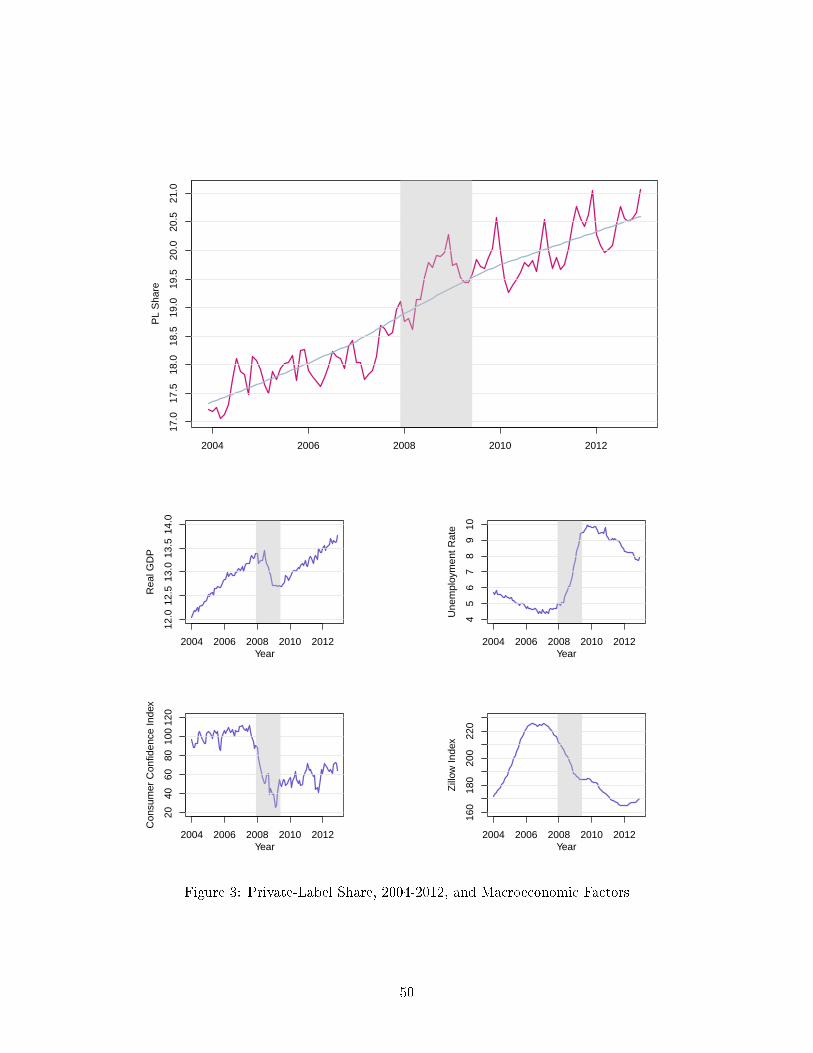
2004 2006 2008 2010 2012

PL

Sha

re

17.0

17.5

18.0

18.5

19.0

19.5

20.0

20.5

21.0

2004 2006 2008 2010 2012

12.0

12.5

13.0

13.5

14.0

Rea

l GD

P

Year2004 2006 2008 2010 2012

45

67

89

10

Une

mpl

oym

ent R

ate

Year

2004 2006 2008 2010 2012

2040

6080

100

120

Con

sum

er C

onfid

ence

Inde

x

Year2004 2006 2008 2010 2012

160

180

200

220

Zill

ow In

dex

Year

Figure 3: Private-Label Share, 2004-2012, and Macroeconomic Factors

50

2006

2009

<44-55-77-99-1111-1313-15>15

Figure 4: Unemployment Rate by FIPS County, 2009 vs. 2006

51

Difference in unemployment

Den

sity

−10 −5 0 5 10 15

0.00

0.05

0.10

0.15

Difference in log Zillow index

Den

sity

−1.0 −0.5 0.0 0.5

0.0

0.5

1.0

1.5

2.0

Figure 5: Cross-Sectional Di�erences in Unemployment Rates (FIPS County Code) and (log) ZillowHome Values (ZIP Code), December 2009 vs. January 2006

52

Log National Brand/Private Label Price Ratio Change

Den

sity

0

20

40

60

−0.04 −0.02 0.00 0.02 0.04

2009 2010

−0.04 −0.02 0.00 0.02 0.04

2011

2007

−0.04 −0.02 0.00 0.02 0.04

0

20

40

60

2008

Figure 6: Regional National-Brand/Private-Label Price Changes

Note: The panels show yearly log changes in the relative national-brand/private-label price index,log(PNB,t/PPL,t)− log(PNB,t−1/PPL,t−1), between year t− 1 and year t. The observations are at the DMAlevel, and the regional price indices are constructed using regional category expenditure weights.

53

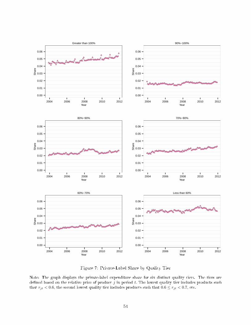
0.00

0.01

0.02

0.03

0.04

0.05

0.06

2004 2006 2008 2010 2012Year

Sha

re

Greater than 100%

0.00

0.01

0.02

0.03

0.04

0.05

0.06

2004 2006 2008 2010 2012Year

Sha

re

80%−90%

0.00

0.01

0.02

0.03

0.04

0.05

0.06

2004 2006 2008 2010 2012Year

Sha

re

60%−70%

0.00

0.01

0.02

0.03

0.04

0.05

0.06

2004 2006 2008 2010 2012Year

Sha

re

90%−100%

0.00

0.01

0.02

0.03

0.04

0.05

0.06

2004 2006 2008 2010 2012Year

Sha

re

70%−80%

0.00

0.01

0.02

0.03

0.04

0.05

0.06

2004 2006 2008 2010 2012Year

Sha

re

Less than 60%

Figure 7: Private-Label Share by Quality Tier

Note: The graph displays the private-label expenditure share for six distinct quality tiers. The tiers arede�ned based on the relative price of product j in period t. The lowest quality tier includes products suchthat rjt < 0.6, the second lowest quality tier includes products such that 0.6 ≤ rjt < 0.7, etc.

54

1000

2000

3000

4000

2006 2007 2008 2009 2010 2011 2012Year

Pro

duct

Cou

nt

National BrandPrivate Label

Number of New Products

Figure 8: New Private-Label and National-Brand Product Introductions

55

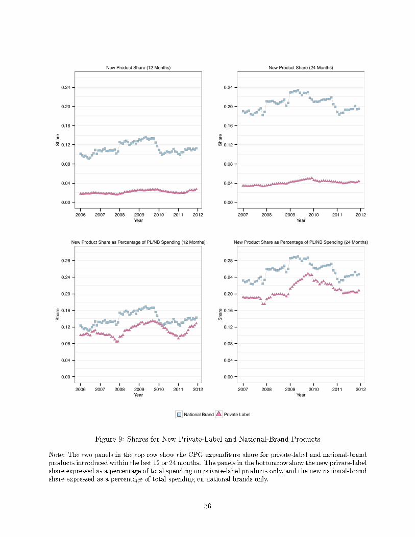
0.00

0.04

0.08

0.12

0.16

0.20

0.24

2006 2007 2008 2009 2010 2011 2012Year

Shar

e

New Product Share (12 Months)

0.00

0.04

0.08

0.12

0.16

0.20

0.24

2007 2008 2009 2010 2011 2012Year

Shar

e

New Product Share (24 Months)

0.00

0.04

0.08

0.12

0.16

0.20

0.24

0.28

2006 2007 2008 2009 2010 2011 2012Year

Shar

e

New Product Share as Percentage of PL/NB Spending (12 Months)

0.00

0.04

0.08

0.12

0.16

0.20

0.24

0.28

2007 2008 2009 2010 2011 2012Year

Shar

e

New Product Share as Percentage of PL/NB Spending (24 Months)

National Brand Private Label

Figure 9: Shares for New Private-Label and National-Brand Products

Note: The two panels in the top row show the CPG expenditure share for private-label and national-brandproducts introduced within the last 12 or 24 months. The panels in the bottomrow show the new private-labelshare expressed as a percentage of total spending on private-label products only, and the new national-brandshare expressed as a percentage of total spending on national brands only.

56

0.0

0.1

0.2

0.3

2006 2007 2008 2009 2010 2011 2012Year

Sha

re

Greater than 100%

0.0

0.1

0.2

0.3

2006 2007 2008 2009 2010 2011 2012Year

Sha

re

80%−90%

0.0

0.1

0.2

0.3

2006 2007 2008 2009 2010 2011 2012Year

Sha

re

60%−70%

0.0

0.1

0.2

0.3

2006 2007 2008 2009 2010 2011 2012Year

Sha

re

90%−100%

0.0

0.1

0.2

0.3

2006 2007 2008 2009 2010 2011 2012Year

Sha

re

70%−80%

0.0

0.1

0.2

0.3

2006 2007 2008 2009 2010 2011 2012Year

Sha

re

Less than 60%

Figure 10: Share of New Products Within Each Quality Tier (12 Months)

Note: The graph shows the new private-label product share as a percentage of total spending within eachof the six distinct quality tiers. New products include all products introduced within the last 12 months.

57

0.00

0.25

0.50

0.75

1.00

0.00 0.25 0.50 0.75 1.00New Products

New

Pro

duct

Sal

es

2006

0.00

0.25

0.50

0.75

1.00

0.00 0.25 0.50 0.75 1.00New Products

New

Pro

duct

Sal

es

2007

0.00

0.25

0.50

0.75

1.00

0.00 0.25 0.50 0.75 1.00New Products

New

Pro

duct

Sal

es

2008

0.00

0.25

0.50

0.75

1.00

0.00 0.25 0.50 0.75 1.00New Products

New

Pro

duct

Sal

es

2009

0.00

0.25

0.50

0.75

1.00

0.00 0.25 0.50 0.75 1.00New Products

New

Pro

duct

Sal

es

2010

0.00

0.25

0.50

0.75

1.00

0.00 0.25 0.50 0.75 1.00New Products

New

Pro

duct

Sal

es

2011

Private Label National Brand

Figure 11: New Product Share Concentrated Among Top Selling Products

Note: The graph shows the percentage of new private-label or national-brand product revenue that isaccounted for by the top N percent of all products, ranked according to total 12-month revenue afterproduct launch.

58

Appendices

A Derivation of the Lower-Level AIDS Demand System

Suppose a household has the following separable utility function over k = 1, ...,K commodity groups

including CPG:

u = f [v1 (q1) , ..., vCPG (qCPG) , ..., vK (qK)] (10)

where vi (qi) is the sub-utility associated with consumption level qi in commodity group i.

Recall from equation 3 of section 6.1, we follow the convention in the literature (e.g. Hausman,

Leonard, and Zona 1994) and model the budget allocation to the CPG commodity group as follows:

:

log(yCPG) = η + δI log(I) + δW log(W ) +K∑k=1

αk log(Pk) + ν (11)

where Pk is the price index for commodity group k.

We now provide a derivation of the AIDS speci�cation used to model lower-level demand in the

CPG commodity group. The CPG group consists of two products, private label (PL) and national

brand (NB). We denote the CPG price vector as P = (PPL, PNB)′ . A household has the following

expenditure function over these CPG products

e (u, P ) = minqCPG [qPLPPL + qNBPNB|vCPG (qCPG) = u] . (12)

which generates a CPG indirect utility function

u = ψ (yCPG, P ) (13)

where yCPG is the budget the household allocates to the CPG category.

We specify the PIGLOG (price independent generlized linearity) �exible functional form to

approximate the expenditure function:

lne (u, P ) = ub (P ) + (1− u) a (P ) (14)

where

a (P ) = α0 + αPLlnpPL + αNBlnPNB + 12γPL,PLlnP

2PL + 1

2γNB,NBlnP2NB + γPL,NBlnPPLlnPNB

b (P ) = a (P ) + β0PβPLPL P βNBNB

and homogeneity in P implies the following parameter restrictions:

59

αPL = 1− αNBβPL = −βNB

γPL,NB + γNB,NB = 0

γPL,PL + γPL,NB = 0.

. (15)

We impose the restrictions in (15) and then derive the expenditure share for PL

sPL ≡∂lne (u, P )

∂lnPPL= αPL + γln

(PPLPNB

)+ βPLuβ0P

βPLPL P βNBNB

where γPL,PL = γNB,NB = γ. We can simplify by inverting out u from (14):

u =lnyCPG −

[α0 + αPLlnPPL + αNBlnPNB + 1

2γPL,PLlnP2PL + 1

2γNB,NBlnP2NB + γPL,NBlnPPLlnPNB

]β0P

βPLPL P βNBNB

.

(16)

Substituting (16) back into the share equation, we obtain:

sPL = αPL + γln

(PPLPNB

)+ βPLln

(yCPGPCPG

)(17)

where the theoretical CPG price index, PCPG, is given by:

lnPCPG = α0+αPLlnPPL+αNBlnPNB+1

2γPL,PLlnP

2PL+

1

2γNB,NBlnP

2NB+γPL,NBlnPPLlnPNB.

(18)

In our analysis, we follow the convention in the literature and use the Stone Price index to approx-

imate equation 18 (e.g. Deaton and Muellbauer 1980b; Hausman, Leonard, and Zona 1994).

B Price index construction

To estimate the private-label expenditure share equation (5) we need to construct price indices.

Using the Homescan data to construct these indices is di�cult because we only observe prices

conditional on a household purchase. Correspondingly, the price observations for any given product

in a store are sparse, and the sampled prices do not re�ect the true price levels that households

face because a purchase is more likely at a relatively low, possibly promoted price. Instead, we

calculate the price indices using price observations from the Nielsen RMS (Retail Management

System) scanner data. The price series in the RMS data are much less sparse because prices are

recorded in any given week whenever at least one unit of a product is sold. For weeks when the sales

quantity is zero we impute the shelf price as the most recent base (non-promoted) price, which we

predict using an algorithm that we developed to classify prices as base or promoted prices. Since our

store sample does not include all stores, excluding for instance Walmart, we cannot construct the

exact price indices corresponding to each household's purchase basket. Instead, we �rst calculate

60

regional category-level price indices. We then calculate household-level price indices by aggregating

over the category-level indices using household-level category expenditure weights.

The �rst step is to calculate store-level category price indices. We index stores by s and categories

by k. The category k price index πkst is then de�ned as a weighted geometric average:

πkstπks,t−1

=∏

j∈Jkst

(pjstpjs,t−1

)ωjr. (19)

Jkst is the set of products in category k and store s that are available at time t and t− 1, and pjst

in the price of product j ∈ Jkst. ωjr is the average expenditure share of product j in the region r

where the store is located.26

In the second step we calculate regional category price indices πkrt :

πkrtπkr,t−1

=∏

s∈Skrt

(πkstπks,t−1

)ωsr. (20)

Skrt is the set of stores carrying products in category k in region r, and ωsr is a store size weight

based on the total average weekly revenue (across all categories) in store s.27 We choose the 205

DMA's in our sample as regions. We make this choice to balance the competing goals of (i) ensuring

that the regional price indices are based on a su�cient number and variety of stores and (ii) allowing

for su�cient price variation across local regions.

In the third step we then calculate household-speci�c price indices Pht :

PhtPh,t−1

=∏k∈Ih

(πkrtπkr,t−1

)ωkh. (21)

Ih is the set of categories in which household h ever purchases and ωkh is a household-speci�c cate-

gory expenditure weight. Note that Pht is customized to re�ect the spending patterns of household

h across product categories based on region-speci�c, not household-speci�c category price levels.

We create versions of Pht for all CPG products and separately for national-brand and private-

label products. We also use data on purchases in the �General Merchandise� department, which

we do not include in the de�nition of CPG products, to create an upper level price index for the

General Merchandise product group. Finally, we proxy for a product group including all other items

using the regional consumer price index (CPI) from the Bureau of Labor Statistics. The CPI is a

geometric-weight price index and hence approximately satis�es

log(PCPI) = ω1 log(P1) + ω2 log(P2) + ω3 log(P3),

where 1 is an index for the CPG product group, 2 is an index for the General Merchandise product

group, and 3 represents the product group of �all other� items. Hence, log(P3) can be represented

26In general, not all products are sold in store s at time t and t− 1, and hence the weights ωjr are renormalized tosum to one. Therefore, to be entirely concise, the weights should be indexed as ωjkst.

27Like the product weights, the store size weights are renormalized to sum to one.

61

as a linear combination of the log of the CPI and the log of the CPG and General Merchandise price

indices. We can therefore include the log CPI instead of the �all other� product group price index

in the upper level demand model and the private-label share equation, although this will change

the interpretation of the estimated price index parameters.

C Additional Lower-Level Demand Estimates

In this appendix, we provide our lower-level demand model estimated with prices indices that have

�xed regional weights (as opposed to the household-speci�c weights used above). We also provide

estimate of the lower-level demand for food products only.

62

Table 14: Lower Level Demand: AIDS Private-Label-Share System (Food Only)

within +

recession

+ trend

CPG

prices

CPG

prices +

proxies

log(Income) -0.361 -0.317 -0.316

(0.072) (0.0781) (0.0778)

log(Wealth) -0.755 -0.264 -0.254

(0.157) (0.184) (0.184)

I{Unemployed} 0.341 0.282 0.288

(0.0908) (0.0996) (0.0999)

Trend 0.0338 0.0217 0.0296

(0.00182) (0.00433) (0.00489)

I{Recession} 0.39 -0.009 0.00379

(0.0477) (0.0527) (0.0552)

I{Post Recession} 0.183 -0.308 -0.411

(0.0865) (0.104) (0.107)

Trend× I{Recession} 0.00538 -0.018 -0.0242

(0.00471) (0.0055) (0.00624)

Trend× I{Post Rec.} -0.0241 -0.00247 -0.0139

(0.00433) (0.00597) (0.00645)

log(PI National Brand) 14.7 15.1

(2.36) (2.39)

log(PI Private Label) 0.739 0.439

(1.27) (1.26)

log(PI All CPG) -2.34 -2.11

(2.43) (2.49)

log(CPI) -2.12

(1.11)

log(PI Gen. Merchandise) -2.84

(0.759)

Fixed E�ects HH HH HH

No. Obs. 1,716,947 1,335,083 1,317,535

No. Missing 3,185,575 3,567,439 3,584,987

No. Clusters 39,413 36,021 35,972

R2 0.576 0.583 0.585

63

Table 15: Upper Level Demand: CPG Expenditure System (food only)

CPG

prices

only

CPG

prices +

price

proxies

CPG

prices +

price

proxies +

trend

CPG

prices +

price

proxies +

trend+ 4

income

lags

log(Income) 0.0258 0.0236 0.0244 0.025

(0.0039) (0.00389) (0.00387) (0.00442)

log(Wealth) 0.0433 0.0227 0.0111 0.00632

(0.00812) (0.00825) (0.00928) (0.0112)

I{Unemployed} -0.00216 -0.00253 -0.00033 0.00915

(0.005) (0.005) (0.00498) (0.00601)

log(Income)−1 0.0453

(0.00479)

log(Income)−2 0.0315

(0.00487)

log(Income)−3 0.0178

(0.00514)

log(Income)−4 0.00448

(0.00479)

log(PI All CPG) 0.535 0.906 0.319 0.352

(0.0307) (0.0411) (0.0609) (0.0725)

log(PI Gen. Merchandise) 0.0494 -0.126 -0.13

(0.0324) (0.0349) (0.0423)

log(CPI) -0.782 -1.72 -1.78

(0.0463) (0.0613) (0.0776)

Trend 0.00602 0.00585

(0.000253) (0.000293)

I{Recession} 0.0456 0.0428

(0.0028) (0.00356)

I{Post Recession} -0.0908 -0.0809

(0.00502) (0.00579)

Trend× I{Recession} -0.00645 -0.00603

(0.000298) (0.000356)

Trend× I{Post Rec.} -0.00602 -0.00552

(0.000322) (0.000371)

Fixed E�ects HH HH HH HH

No. Obs. 1,332,396 1,314,940 1,314,940 897,747

No. Missing 3,570,126 3,587,582 3,587,582 4,004,775

No. Clusters 36,021 35,972 35,972 24,441

R2 0.573 0.576 0.576 0.582

64

Table 16: Lower Level Demand: AIDS Private-Label-Share System (Region Weighted Price Index)

within +

recession

+ trend

CPG

prices

CPG

prices +

proxies

log(Income) -0.412 -0.376 -0.382

(0.0654) (0.0717) (0.0712)

log(Wealth) -0.545 -0.162 -0.202

(0.141) (0.164) (0.164)

I{Unemployed} 0.373 0.34 0.352

(0.0812) (0.0905) (0.0907)

Trend 0.0372 0.0415 0.0518

(0.00159) (0.00467) (0.00514)

I{Recession} 0.322 0.202 0.123

(0.0427) (0.0465) (0.0499)

I{Post Recession} 0.479 0.202 0.0553

(0.0769) (0.117) (0.122)

Trend× I{Recession} 0.019 0.00591 0.00602

(0.00419) (0.00648) (0.00733)

Trend× I{Post Rec.} -0.029 -0.0277 -0.0601

(0.0039) (0.00586) (0.00681)

log(PI National Brand) 9.99 10.8

(7.09) (7.18)

log(PI Private Label) 5.7 4.86

(2.37) (2.37)

log(PI All CPG) -10.6 -9.83

(8.23) (8.29)

log(CPI) -1.53

(1.03)

log(PI Gen. Merchandise) -10.7

(1.18)

Fixed E�ects HH HH HH

No. Obs. 1,716,947 1,335,207 1,317,596

No. Missing 3,185,575 3,567,315 3,584,926

No. Clusters 39,413 36,022 35,973

R2 0.57 0.576 0.578

65

Table 17: Upper Level Demand: CPG Expenditure System (Region Weighted Price Index)

CPG

prices

only

CPG

prices +

price

proxies

CPG

prices +

price

proxies +

trend

CPG

prices +

price

proxies +

trend+ 4

income

lags

log(Income) 0.0283 0.0267 0.0266 0.0238

(0.0037) (0.00369) (0.00369) (0.0042)

log(Wealth) 0.0601 0.0444 0.0156 0.00942

(0.00794) (0.00807) (0.00895) (0.0107)

I{Unemployed} -0.00512 -0.00442 -0.00277 0.0083

(0.00465) (0.00462) (0.0046) (0.0056)

log(Income)−1 0.0451

(0.00438)

log(Income)−2 0.0333

(0.00446)

log(Income)−3 0.0166

(0.00454)

log(Income)−4 0.00406

(0.00445)

log(PI All CPG) 0.41 1.04 0.528 0.627

(0.0303) (0.0435) (0.074) (0.0876)

log(PI Gen. Merchandise) 0.075 -0.495 -0.54

(0.0481) (0.0585) (0.068)

log(CPI) -1.08 -1.73 -1.77

(0.045) (0.0593) (0.0735)

Trend 0.00478 0.00451

(0.00026) (0.000301)

I{Recession} 0.0445 0.0387

(0.00269) (0.00344)

I{Post Recession} -0.0702 -0.0627

(0.00478) (0.0055)

Trend× I{Recession} -0.00598 -0.00542

(0.000284) (0.000336)

Trend× I{Post Rec.} -0.00633 -0.00576

(0.000353) (0.000405)

Fixed E�ects HH HH HH HH

No. Obs. 1,334,612 1,317,015 1,317,015 899,050

No. Missing 3,567,910 3,585,507 3,585,507 4,003,472

No. Clusters 36,022 35,973 35,973 24,441

R2 0.578 0.58 0.581 0.586

66

Table 18: Lower Level Demand: AIDS Private-Label-Share System (Food Only and RegionWeighted Price Index)

within +

recession

+ trend

CPG

prices

CPG

prices +

proxies

log(Income) -0.361 -0.314 -0.316

(0.072) (0.078) (0.0777)

log(Wealth) -0.755 -0.233 -0.262

(0.157) (0.184) (0.184)

I{Unemployed} 0.341 0.282 0.287

(0.0908) (0.0995) (0.0999)

Trend 0.0338 0.0399 0.0517

(0.00182) (0.00513) (0.00559)

I{Recession} 0.39 -0.0242 -0.0161

(0.0477) (0.0534) (0.0558)

I{Post Recession} 0.183 -0.314 -0.477

(0.0865) (0.106) (0.109)

Trend× I{Recession} 0.00538 -0.0151 -0.0204

(0.00471) (0.00575) (0.00644)

Trend× I{Post Rec.} -0.0241 -0.0196 -0.0524

(0.00433) (0.0065) (0.00743)

log(PI National Brand) 32.1 23.5

(4.03) (4.1)

log(PI Private Label) 6.71 3.87

(2) (2.03)

log(PI All CPG) -33.2 -19.7

(5.93) (6.07)

log(CPI) -3.45

(1.13)

log(PI Gen. Merchandise) -10.5

(1.36)

Fixed E�ects HH HH HH

No. Obs. 1,716,947 1,335,083 1,317,535

No. Missing 3,185,575 3,567,439 3,584,987

No. Clusters 39,413 36,021 35,972

R2 0.576 0.583 0.585

67

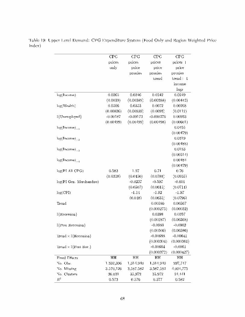
Table 19: Upper Level Demand: CPG Expenditure System (Food Only and Region Weighted PriceIndex)

CPG

prices

only

CPG

prices +

price

proxies

CPG

prices +

price

proxies +

trend

CPG

prices +

price

proxies +

trend+ 4

income

lags

log(Income) 0.0265 0.0246 0.0242 0.0249

(0.0039) (0.00388) (0.00388) (0.00442)

log(Wealth) 0.0506 0.0353 0.0072 0.00268

(0.00826) (0.00839) (0.0093) (0.0112)

I{Unemployed} -0.00187 -0.00173 -0.000276 0.00933

(0.00499) (0.00499) (0.00498) (0.00601)

log(Income)−1 0.0455

(0.00479)

log(Income)−2 0.0319

(0.00488)

log(Income)−3 0.0183

(0.00514)

log(Income)−4 0.00484

(0.00479)

log(PI All CPG) 0.583 1.27 0.71 0.76

(0.0318) (0.0456) (0.0788) (0.0935)

log(PI Gen. Merchandise) -0.0237 -0.597 -0.601

(0.0507) (0.0615) (0.0714)

log(CPI) -1.14 -1.92 -1.97

(0.048) (0.0635) (0.0796)

Trend 0.00586 0.00567

(0.000275) (0.00032)

I{Recession} 0.0398 0.0357

(0.00287) (0.00368)

I{Post Recession} -0.0989 -0.0902

(0.00506) (0.00586)

Trend× I{Recession} -0.00688 -0.00641

(0.000304) (0.000361)

Trend× I{Post Rec.} -0.00664 -0.0061

(0.000372) (0.000427)

Fixed E�ects HH HH HH HH

No. Obs. 1,332,396 1,314,940 1,314,940 897,747

No. Missing 3,570,126 3,587,582 3,587,582 4,004,775

No. Clusters 36,021 35,972 35,972 24,441

R2 0.573 0.576 0.577 0.582

68