Dynamic Labor Demand in China: Public and Private...

Dynamic Labor Demand in China: Public and Private

Objectives∗

Russell Cooper†and Guan Gong‡and Ping Yan §

March 14, 2011

Abstract

This paper studies dynamic labor demand of private and state-controlled manu-

facturing plants in China. A goal of the paper is to characterize adjustment costs for

these plants. As our sample includes private and state-controlled plants, our analy-

sis uncovers differences in both objectives and adjustment costs across these types of

plants. We find evidence of both quadratic and firing costs at the plant level. The

private plants operate with lower quadratic adjustment costs. The higher quadratic

adjustment costs of the state-controlled plants may reflect their internalization of social

costs of employment adjustment. State-controlled plants appear to be maximizing the

discounted present value of profits without a soft-budget constraint. Private plants

discount the future more than state-controlled plants.

∗We are grateful to conferences participants at the 2010 Shanghai Macroeconomics Workshop at SUFE,

the Tsinghua Workshop in Macroeconomics 2010 and the ESWC 2010. This research was supported by a

National Science Foundation (# 0819682) to Russell Cooper and a National Science Foundation of China

grant (# 70903004) to Ping Yan and Russell Cooper. The Department of Social Science of Peking Uni-

versity provided additional research funding. Guan Gong also benefited from the support of the Leading

Academic Discipline Program, 211 Project for Shanghai University of Finance and Economics (the 3rd phase)

and Shanghai Leading Academic Discipline Project (# B801). Huabin Wu provided outstanding research

assistance.†Department of Economics, European University Institute and Department of Economics, University of

Texas at Austin, [email protected]‡School of Economics, Shanghai University of Finance and Economics§CCER, National School of Development, Peking University

1

1 MOTIVATION

1 Motivation

This paper studies dynamic labor demand of private and state-controlled manufacturing

plants in China.1 These results can be used to study a wide variety of policy interventions,

such as labor market regulations and the relaxation of financial market constraints, which

impact directly on factor demand at the plant-level. To predict the effects of these and other

interventions requires answers to two fundamental questions: (i) what are the adjustment

costs faced by plants in China and (ii) what are the objectives of plant managers? This

paper answers both of these questions.

There are a couple of features making this analysis unique. First, our attention is on

plants in China rather than labor market aggregates. Second, the Chinese data include both

private and state-controlled enterprises (SCE). While it is natural to assume the privately

owned plants maximize profits, the objective of a SCE is less clear. Our approach is to

specify a couple of alternative objectives and determine which one better matches pertinent

data facts.

We estimate the costs of labor adjustment and the objectives of private plants and SCE

using a simulated method of moments (SMM) approach. The idea is to use some key moments

of labor input, output and productivity at the plant level to infer the parameters of the

dynamic optimization problems.

In looking at the behavior of private and SCE, there are some striking similarities. First,

the SCE, like the private plants, appear to be maximizing the discounted expected value of

profits. Importantly, labor demand is not a static decision: adjustment costs are present and

imply forward looking behavior by plants. Second, the costs of adjusting hours is relatively

small for all plants though higher for private than SCEs. Third, the best fitting model entails

a non-convex firing cost along with linear and quadratic adjustment costs. For both types

of plants, this non-convex adjustment cost applies if job destruction rates exceed 20%.

However, there are some notable differences. The quadratic adjustment costs are much

larger for the SCE, perhaps reflecting an internalized gain to employment stability. The cost

of adjusting hours is also lower for the public plants.

Finally, public plants discount considerably less than do private plants. For our analysis,

1As discussed in section 3, a state-controlled plant is determined by sharing holdings rather than regis-

tration. We sometimes refer to these as public plants as well.

2

2 DYNAMIC OPTIMIZATION PROBLEM

this is not an assumption but is instead a result of our estimation.

In terms of the objective of the SCE, they are best described as profit maximizers with an

added quadratic cost of employment adjustment. We allow public plants to operate under a

soft budget constraint where profits are non-negative. This does not improve the fit of the

model.

2 Dynamic Optimization Problem

This section discusses the dynamic optimization problems for the privately owned plants and

SCEs. The generic dynamic optimization problem is

V (A, e−1) = maxh,e

Γ(A, e, h, e−1) + βEA′|AV (A′, e) (1)

for all (A, e−1). Employment adjustment is assumed to be completed within a period. The

function V (A, e−1) is the value function of a plant continuing in operation.2 The state vector

contains two elements: A is stochastic profitability of the plant and e−1 is the stock of workers

in the previous period. The control variables are the hours worked per worker, h, and the

number of workers for the current period, e.

The function Γ(A, e, h, e−1) represents the current payoff to the plant. Imbedded in this

function are the adjustment costs as well as the objective function. Ultimately, the differences

between privately owned plants and SCE are captured by this function.

2.1 Privately Owned Plant

The generic model in (1) can be tailored to study a privately-owned profit maximizing

plants.3 The objective function for a privately-owned plant is

Γ(A, e, h, e−1) = R(A, e, h)− ω(e, h)− C (A, e−1, e, h) . (2)

Here R(A, e, h) is the revenue flow of a plant employing e workers, each working h hours in

profitability state A. The revenue function has the form

2At this stage, we do not consider entry and exit decisions.3The model follows the approach of Cooper, Haltiwanger, and Willis (2004) study of dynamic labor

demand for privately-owned US plants. A main difference emerges in modeling the behavior of the SCEs.

3


R(A, e, h) = A(eh)α. (3)

This revenue function is the product of a production function, defined over the total labor

input eh, and the demand curve facing the plant. The parameter α captures the curvature

of the production process along with the elasticity of demand. Other factors of production,

which are assumed not to entail any adjustment costs, are chosen optimally as well but are

implicit in revenue and thus in the optimization problem we study.4

The function ω(e, h) in (2) is total compensation paid to the e workers each working h

hours. The compensation function takes the form

ω(e, h) = e(ω0 + ω1hζ). (4)

The parameters characterizing this function will be part of our estimation.5

The cost of adjusting the stock of workers is given by C (A, e−1, e, h). Following Cooper,

Haltiwanger, and Willis (2004), we consider a cost of adjustment function given by:

C (A, e−1, e, h) = F+ + γ+(e− e−1) +ν

2

(e− e−1

e−1

)2

e−1 + (1− λ+)R(A, e, h) (5)

if there is job creation e > e−1. Similarly

C (A, e−1, e, h) = F− + γ−(e−1 − e) +ν

2

(e− e−1

e−1

)2

e−1 + (1− λ−)R(A, e, h) (6)

if there is job destruction e < e−1.

If e = e−1, so there are no net changes in employment, then C (A, e−1, e, h) ≡ 0. This

specification assumes that there are no costs of filling a vacancy created by a quit. Put

4That is, one can think of R(A, e, h) as the revenue obtained less the costs of the other inputs. Since

the quantities of those other inputs are dependent on (A, e, h), the R(A, e, h) captures these choices. The

functional form in (3) can be derived from a plant optimization problem over flexible factors with a constant

returns to scale technology and a constant elasticity demand curve for plant output.5This functional form is often used to characterize compensation, including overtime, in US data. The

Chinese Labor Law enacted in 1995 stipulates that employees work no more than 8 hours per day, and no

more than 44 hours per week. In addition, overtime hourly pay needs to be no less than: 1.5 times straight-

hour pay on weekdays; 2 times on Saturday and Sunday; 3 times on national holidays. The functional form

provides a smooth approximation to these requirements. For further discussion of compensation functions

and their representation see Bils (1987).

4


differently, the adjustment costs are on net not gross employment changes. This assumption

is consistent with the observation of zero net employment changes at a significant fraction

of plants.

There are four forms of adjustment costs, with differences allowed for the job creation

and job destruction margins. The first is a quadratic adjustment cost, parameterized by

ν. There are two types of non-convex costs considered. One, parameterized by λ is an

opportunity cost of adjustment: the plant losses a fraction (1 − λ) of its revenues when it

adjusts its labor force. A second, parameterized by F , is a more traditional fixed cost of

adjusting the work force. In previous work on labor adjustment, Cooper, Haltiwanger, and

Willis (2004) found evidence in U.S. plants in favor of the opportunity cost model relative

to the fixed cost form of non-convex adjustment costs. Finally, we allow linear adjustment

costs, parameterized by γ to capture, for example, severance payments to workers. Here we

will study how well each of them matches key features of the data.

In addition to the differences in adjustment costs of hiring and firing workers, this study

adds another feature: the use of thresholds for the non-convex adjustment costs. So, as a

leading example, the fixed cost of firing (F−) may apply only if the job destruction rate ex-

ceeds a bound. Through this modification of (6), we are able to capture certain institutional

features that may generate nonlinearities in adjustment costs.

The optimization generates choices along a couple of dimensions. First there is the

discrete choices of job creation, job destruction or inaction. The latter is an important

option given plant-level observations of no net employment changes. Second, there is the

continuous choice of job creation (destruction). If the job creation (destruction) rates exceed

the threshold, additional non-convex adjustment costs might apply. Third, there is the

adjustment of hours. Variations in hours will reflect both the state of profitability and the

choices on the extensive and intensive employment margins. If there is an opportunity cost

of employment adjustment, so that either (1− λ−) < 1 or (1− λ+) < 1, then the decreased

productivity will also affect the hours choice.

5


2.2 State-Controlled Enterprise

The dynamic optimization problem for a SCE is potentially different from (1). The idea is

to infer the objectives of these enterprises from their actions.6

The key difference we highlight is in the objective function of the SCE. In general, the

objective of the SCE is given by:

Γ(A, e, h, e−1) + S(A, e, h, e−1) (7)

Here Γ(A, e, h, e−1) is the same as in (2). Profits are here both because a SCE could

be interested in maximizing profit and also because tax revenues flow to state and local

governments. The second term in the objective function, S(A, e, h, e−1), covers objectives of

the SCE beyond profit maximization.

We consider a couple of models of S(A, e, h, e−1). The first, termed the “employment

stabilizer”, asserts that the SCE is interested in employment stability. Thus there is an

additional cost, beyond the adjustment cost already included in Γ(A, e, h, e−1) of employment

variability. In this case,

S(A, e, h, e−1) = −νS

2

(e− e−1

e−1

)2

e−1. (8)

In this specification, the cost of employment adjustment is parameterized by νS. This term

is exactly like the quadratic adjustment cost term already included in Γ(A, e, h, e−1) through

C(A, e, e−1). Hence the quadratic cost of adjustment for a SCE is straightforward to estimate

and compare to the adjustment costs for private plants.

A second model, termed the “job creator” adds a benefit of job creation to the SCE’s

objective function and penalizes the SCE for job losses. In this case,

S(A, e, h, e−1) = F+ (9)

when e > e−1 and

S(A, e, h, e−1) = F− (10)

6A similar approach underlies Gowrisankaran and Town (1997) who study the behavior of not-for-profit

hospitals, and estimate an objective function which includes both profits and quality. Sapienza (2002) studies

public and private banks in Italy.

6

3 DATA

when e < e−1. If there are gains to job creation and costs to destruction, we would expect:

F+ > 0 along with F− < 0.

In many descriptions of SCE, the theme of a “soft budget constraint” arises. One inter-

pretation of this is that by following other objectives, imbedded in S(·), the SCE may in fact

operate in a non-profitable fashion.7 In that case, the government may provide a subsidy.

We model this by assuming that the first term in the objective function (1) is given by

Γ(A, e, h, e−1) = max{0,Γ(A, e, h, e−1)} (11)

where Γ(A, e, h, e−1) is defined in (2). With this subsidization, the SCE can undertake other

objectives, such as employment stability, without incurring sustained losses. Further, under

this objective, the SCE has no incentive to exit.

Finally, we estimate the discount factor for both private plants and SCEs. As suggested

by Cull and Xu (2005), it might be that SCEs operate with subsidized loans, from banks and

the government, which leads to them to discount less than private plants. This is potentially

a very interesting and important difference between plants.

Our approach is to estimate the parameters for these specification of the SCE objective.

In some cases, we use the estimates from the profit maximizing plants to create a baseline

and to attribute SCE patterns of dynamic labor demand that differ from those of private

profit maximizing plants to these difference in objectives.

3 Data

The data are from Annual Surveys of Industrial Production (1998-2007), conducted by the

National Bureau of Statistics (NBS) of China. The raw data consist of all private plants

with more than five million Yuan in revenue (about $700,000) and all public plants.8

7This draws upon the discussion of soft budget constraints in Lin and Li (2008). In that analysis, the

state imposes a “policy burden” on a SCE, such as employment stability, and must support the SCE in order

for it to remain in operation.8Each observation in the raw data has a unique physical address. For example, in 2006, 17 observations

in 17 different locations, share the brand name of one of the biggest dairy product makers, Mengniu. Brandt,

Biesebroeck, and Zhang (2009) study productivity at the firm level over the 1998-2006 period. The data are

similar though since they note that about 95% of the firms own a single plant. From Brandt, Biesebroeck,

and Zhang (2009), the cut-off on private plants of five million Yuan in revenues is likely to eliminate less

7

3 DATA

The number of plants grows from over 160,000 in 1998 to above 330,000 in 2007. Since

there are numerous mergers, acquisitions, entry and exit, and public-to-private transforma-

tions before 2005, we focus on a balanced panel of plants excluded from the above changes

and in operation during the period 2005-2007.9 Another reason to look at the data after

2005 is that the year 2004 is characterized by many economic policies at the macro level to

curb the overheating of the economy.

The classification of the plants as public or private is an important element in our anal-

ysis. The Annual Surveys of Industrial Production has two variables defining whether an

enterprise is public or private. One is “enterprise type”, representing state-owned, collective,

domestic private, joint venture, and foreign (including Hong Kong, Macao and Taiwan) pri-

vate enterprises. State-owned means the enterprise is owned by all the people in the country,

while collective means the enterprise is owned by part of the people in the country. Accord-

ing to the Chinese constitution, both state-owned and collective enterprises are classified as

public. An enterprise is termed as a joint venture if part of its shares is owned by foreign

investors or companies, no matter how big the fraction is. Enterprise type is the type that

the enterprise is registered with the Administration of Business and Commerce, as well the

Administration of Taxation. It does not have any information on who among shareholders

makes decisions. The decision maker of a joint venture can be either public shareholders or

private shareholders.

The other variable is “control of shares”, representing state controlled, collectively con-

trolled, domestically privately controlled, and foreign (including Hong Kong, Macao and

Taiwan) privately controlled enterprises. “Control” means holding over 50% of total shares,

or being pivotal in decision making if not holding over 50% of total shares. By this standard,

a joint venture is public if it is state controlled or collectively controlled, even if it is not

registered as a state-owned or collective enterprise according to the enterprise type criterion.

For example, Volkswagen, Ford, and Honda in mainland China are all state-controlled joint

ventures. On the other hand, in our data we do see a large fraction of enterprises that are

registered as collective but are controlled by domestic private shareholders.

To make a clear distinction between public and private, we rely on the variable control

than 1% of the private plants. The analysis of Hsieh and Klenow (2009) covered the 1998-2005 period.9This transformation in manufacturing is summarized in http://www.carnegieendowment.org/

publications/?fa=view&id=22633.

8

3 DATA

of shares to determine the type of an enterprise. In the balanced panel we are looking at,

there are 13,255 state-controlled enterprises and 14,374 collectively-controlled enterprises,

both classified as public. Our private category consists of 120,719 domestically privately

controlled enterprises and 35,466 foreign (including Hong Kong, Macao and Taiwan) privately

controlled enterprises.

Table 1 summarizes capital, employment (number of workers employed), revenue, and

value-added by enterprise type for the 2005-2007 period.10 All monetary terms are deflated to

thousand Yuan in 2005 using CPI. The survey includes a measure of plant-level ”net capital”

constructed using a perpetual inventory method. Hours information is not available.

The columns split the sample into public and private plants. The columns called “trimmed”

are a subsample in which the top and bottom 2.5% of the plants, by employment size, are re-

moved to deal with outliers. For the public plants, the column marked large reports statistics

for this top 2.5% group. Unless stated otherwise, we will focus on the trimmed sample.

About 85% of the sample consists of private plants, most of them are domestic not foreign

owned. In terms of numbers of workers (Emp.), the private plants are typically about half

the size of the public plants. Yet the public plants have value added (VA) and revenue (Rev.)

more than twice that of the private plants. The public plants are also considerably more

capital intensive (Cap./Emp.) on average.

In terms of average revenue per worker, the public plants are more productive than the

private plants on average. The foreign plants have the highest revenue per worker among

private plants but this is still less than the productivity in the large public SCE. In terms of

average revenue per unit of capital, the public plants are about as productive as the private

ones. In fact the revenue per unit of capital is almost identical for the large public SCE and

the foreign private plants.

As noted earlier, we focus on the 2005-07 period to exclude periods of substantial change

in the structure and ownership of plants. For purpose of comparison, Table 2 provides similar

data for public and private plants from an earlier period, 1998. In this earlier period, the

fraction of public plants is 69% of the total, compared to only 15% in the later period.11 The

10Because the Annual Surveys of Industrial Production is a census conducted by the NBS and not by

the Administration of Taxation, we believe the information reported is unlikely to be contaminated by tax

evasion incentives.11This period is reflected in the discussion in Bai, Lu, and Tao (2006) which emphasized the presence of

large relatively inefficient public plants.

9

3 DATA

Public

Pri

vate

Tot

alA

llT

rim

med

Upp

er2.

5%A

llT

rim

med

Dom

esti

cF

orei

gn

#pla

nts

183,

814

27,6

2926

,325

691

156,

185

148,

390

120,

719

35,4

66

Val

ue

added

35,5

3499

,446

48,6

572,

107,

979

24,2

2817

,665

18,1

4644

,931

(357

,553

)(8

50,6

25)

(361

,262

)(4

,448

,673

)(1

47,0

14)

(53,

062)

(96,

231)

(251

,206

)

Rev

enue

124,

270

306,

272

152,

329

6,41

1,03

292

,074

64,2

9066

,417

179,

407

(1,0

59,3

66)

(2,1

34,1

62)

(718

,712

)(1

.11e

+7)

(712

,869

)(2

05,8

42)

(356

,131

)(1

,340

,289

)

Em

plo

ym

ent

284

618

337

11,5

8722

417

218

038

5

(1,6

04)

(3,6

96)

(504

)(2

0,00

3)(7

51)

(190

)(5

69)

(1,1

86)

Cap

ital

46,5

5718

6,77

689

,995

4,01

4,53

421

,752

15,3

9715

,362

43,5

02

(686

,797

)(1

,726

,791

)(5

82,5

36)

(9,5

46,4

31)

(153

,506

)(6

9,20

7)(1

24,9

91)

(223

,570

)

Cap

./E

mp.

125

310

242

308

9288

8013

6

(3,5

28)

(8,9

26)

(4,7

57)

(741

)(6

36)

(430

)(4

22)

(1,1

08)

VA

/Em

p.

144

207

160

209

133

127

127

155

(1,7

30)

(4,3

49)

(1,3

24)

(404

)(3

76)

(309

)(2

77)

(613

)

VA

/Cap

.5.

66

5.4

4.5

5.5

5.3

5.6

5.3

(96)

(118

)(1

09)

(145

)(9

2)(8

9)(8

0)(1

25)

Rev

./E

mp.

504

601

508

688

487

461

467

561

(3,7

08)

(7,4

02)

(2,2

61)

(1,1

39)

(1,1

66)

(1,1

8)(9

34)

(1,7

69)

Rev

./C

ap.

23.5

24.9

22.7

20.3

23.2

22.2

24.1

20.2

(353

)(5

05)

(491

)(5

06)

(319

)(3

12)

(332

)(2

67)

Tab

le1:

Char

acte

rist

ics

ofP

lants

by

typ

e,20

05-2

007

bal

ance

dpan

el.

All

mon

etar

yte

rms

are

in1,

000

RM

B,

defla

ted

to20

05le

vel.

The

trim

med

sam

ple

is

the

publ

ic(p

riva

te)

sam

ple

excl

udin

gth

eup

per

and

low

er2.

5%ta

ilsby

empl

oym

ent

size

.

Stan

dard

devi

atio

nsar

epa

rent

hesi

zed.

10

4 QUANTITATIVE ANALYSIS

public plants in the total sample were larger than private plants in terms of value added,

revenue, employment and capital. The large public enterprises were considerably larger.

Productivity, measured either as the average revenue product of capital or labor was much

lower in public than private plants. This is particularly true for the large SCE, which are

particularly unproductive. These large differences in productivity are not apparent in the

recent sample.

As we shall see as our analysis proceeds, the public plants are not that different from

the private ones. Given the results in Tables 1 and 2, perhaps this reflects privatization and

modernization of public plants.12

4 Quantitative Analysis

The estimation follows two procedures. As in Cooper and Haltiwanger (2006), some of

the parameters are estimated directly from data on revenues. The remainder are obtained

through a simulated method of moments approach.

4.1 Parameter Estimates of Revenue Function

Using data on revenues and the labor input at the plant level for the trimmed sample, we

can estimate α from Rit = AitLαit, where Lit is the total labor input at plant i in period

t.13 In addition, we use these regression results to back-out the profitability shock, Ait, as

a residual and from this we can infer the process for this shock. We then create a discrete

representation of the process as an input in computing conditional expectations for the

dynamic optimization problem at the plant level. This procedure is followed for both public

and private plants.

The results of the IV estimation are shown in Table 3. Here α is the curvature of the

revenue (profit) function and ρ is the serial correlation of the profitability shock process.14

12This is consistent with Table 3 of Brandt, Biesebroeck, and Zhang (2009) though our determination of

private vs. public differs.13These regressions used plant-level wages and initial capital stock to control for some of the plant-level

heterogeneity. For the case of opportunity costs, the estimation included a dummy variable for employment

adjustment to control for the effects of disruption costs. Those results are close to the ones reported in Table

3. The data appendix provides more detailed discussion of this estimation.14Though we use only three years of data, the number of observations used to estimate the serial correlation

11


Public

Pri

vate

Tot

alA

llL

ower

2.5%

Tri

mm

edU

pp

er2.

5%A

llT

rim

med

#pla

nts

134,

947

93,4

552,

298

88,8

252,

332

41,4

9239

,465

Val

ue

added

14,1

4915

,175

2403

8,94

726

4,96

411

,838

9,57

5

(169

,708

)(2

00,7

98)

(17,

605)

(37,

281)

(1,2

24,4

02)

(53,

371)

(27,

667)

Rev

enue

47,3

8547

,960

7,94

030

,383

756,

879

46,0

9137

,056

(326

,117

)(3

68,7

15)

(47,

517)

(95,

051)

(2,1

41,9

35)

(199

,213

)(9

0,88

3)

Em

plo

ym

ent

384

441

8.8

277

7,09

525

620

6

(1,9

72)

(2,3

45)

(2.7

)(3

59)

(13,

038)

(491

)(2

12)

Cap

ital

34,5

3340

,818

4,11

721

,432

815,

391

20,3

7916

,470

(397

,298

)(4

70,7

63)

(47,

914)

(148

,461

)(2

,725

,265

)(1

17,9

82)

(99,

387)

Cap

./E

mp.

9293

1102

6783

8982

(4,0

09)

(4,8

11)

(30,

552)

(431

)(1

48)

(395

)(3

07)

VA

/Em

p.

6259

608

4637

6963

(1,7

51)

(2,1

01)

(13,

348)

(163

)(1

06)

(193

)(1

45)

VA

/Cap

.3.

43.

026.

92.

990.

494.

34.

2

(57)

(38)

(34)

(38)

(0.9

7)(8

6)(8

8)

Rev

./E

mp.

230

208

1,93

416

611

028

125

1

(5,6

11)

(6,7

23)

(42,

699)

(571

)(2

01)

(758

)(5

18)

Rev

./C

ap.

16.4

15.3

28.1

15.3

2.1

18.8

18.4

(307

)(3

41)

(135

)(3

49)

(8)

(214

)(2

18)

Tab

le2:

Char

acte

rist

ics

ofP

lants

in19

98

All

mon

etar

yte

rms

are

in1,

000

RM

B,

defla

ted

to20

05le

vel.

The

trim

med

sam

ple

is

the

publ

ic(p

riva

te)

sam

ple

excl

udin

gth

eup

per

and

low

er2.

5%ta

ilsby

empl

oym

ent

size

.

Stan

dard

devi

atio

nsar

epa

rent

hesi

zed.

12


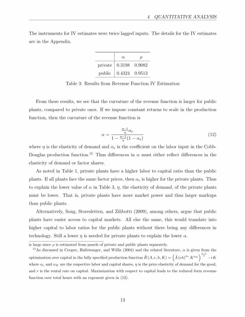
The instruments for IV estimates were twice lagged inputs. The details for the IV estimates

are in the Appendix.

α ρ

private 0.3198 0.9082

public 0.4324 0.9513

Table 3: Results from Revenue Function IV Estimation

From these results, we see that the curvature of the revenue function is larger for public

plants, compared to private ones. If we impose constant returns to scale in the production

function, then the curvature of the revenue function is

α =

η−1ηαe

1− η−1η

(1− αe)(12)

where η is the elasticity of demand and αe is the coefficient on the labor input in the Cobb-

Douglas production function.15 Thus differences in α must either reflect differences in the

elasticity of demand or factor shares.

As noted in Table 1, private plants have a higher labor to capital ratio than the public

plants. If all plants face the same factor prices, then αe is higher for the private plants. Thus

to explain the lower value of α in Table 3, η, the elasticity of demand, of the private plants

must be lower. That is, private plants have more market power and thus larger markups

than public plants.

Alternatively, Song, Storesletten, and Zilibotti (2009), among others, argue that public

plants have easier access to capital markets. All else the same, this would translate into

higher capital to labor ratios for the public plants without there being any differences in

technology. Still a lower η is needed for private plants to explain the lower α.

is large since ρ is estimated from panels of private and public plants separately.15As discussed in Cooper, Haltiwanger, and Willis (2004) and the related literature, α is given from the

optimization over capital in the fully specified production function R (A, e, h,K) =(A (eh)αe KαK

) η−1η −rK

where αe and αK are the respective labor and capital shares, η is the price elasticity of demand for the good,

and r is the rental rate on capital. Maximization with respect to capital leads to the reduced form revenue

function over total hours with an exponent given in (12).

13


Finally, from the perspective of the analysis in Hsieh and Klenow (2009), differences in

capital to labor ratios may reflect different frictions in factor allocation. The higher capital

to labor ratio in public sector would indicate a lower friction in capital relative to labor for

the SCE.

The estimates in Table 3 pertain to data pooled across all sectors of the economy. Sectoral

differences in technology and/or the elasticity of demand could also account for the estimates

reported in Table 3.

The profitability shocks are highly serially correlated for both types of plants. The

processes of the profitability shocks are stationary. Given the costs of hiring and firing

workers, the serial correlation of these shocks is important for the choice between adjusting

hours and the number of workers in response to variations in profitability.

The variability of the shocks to profitability are set to match the size distribution of

plants in the trimmed data set. The minimum size of the plants in the private and public

(trimmed) data set is about 50 workers and the largest is about 1500. The standard deviation

of the shocks, along with the (ω0, ω1) are set to produce an employment distribution within

this range and to match the median establishment size.16

4.2 SMM Estimation Approach

The remained parameters are estimated via SMM. This approach revolves around finding

the vector of structural parameters, denoted Θ, to minimize the weighted difference between

simulated and actual data moments. That is we solve minΘ£(Θ) where

£(Θ) ≡ (Md −M s(Θ))W (Md −M s(Θ))′. (13)

The weighting matrix, W, is obtained by inverting an estimate of the variance/covariance

matrix obtained from bootstrapping the data. The resulting estimator is consistent.17

In this expression, Md are the data moments for private and public plants, M s(Θ) are

the simulation counterparts. The moments are listed as the columns in Tables 5 and 7.

16For the public plants, the standard deviation of the innovation of the profitability shocks is set at 0.45,

which is just about the estimate inferred from the estimation of the revenue functions. For the private plants,

the standard deviation of the innovation is much larger, 0.90, in order to match the size distribution of the

plants. This difference in variability of the shocks appears to stem from the lower value of α in the revenue

function for the private plants.17See, for example, the discussion and references in Adda and Cooper (2003).

14


The std(r/e) is the standard deviation of the log of revenue per worker. The moment sc

is the serial correlation in employment. The distribution of the job creation (JC) and job

destruction (JD) as well as the inaction rate (zero net employment change) are the remaining

seven moments. These are averages across plants and years. The inaction rate of nearly 40%

for the private plants and 28% for the public plants motivates the inclusion of non-convex

adjustment costs.

The simulated moments are obtained by solving the dynamic programming problem in

(1) for a given value of Θ. The resulting decision rules are used to to simulate a panel data

set. The simulated moments are calculated from that data set.18

The parameters estimated by SMM are Θ ≡ (ζ, ν, λ+, λ−, F+, F−, γ+, γ−, β).19 The mo-

ments were selected in part because they are informative about these underlying parameters.

Roughly speaking, the curvature of the compensation function is identified from the standard

deviation of the log of revenue per worker.20 An increase in ζ will lead to a larger varia-

tion in employment relative to hours and thus a reduction in this moment. The quadratic

adjustment cost parameter, ν, is identified largely from variations in the serial correlation

of employment and from the prevalence of employment adjustments in the 10% range. The

distribution of employment changes, particularly the inaction and the large adjustments,

act to pin down the non-convex adjustment costs. Finally, variations in β influence all the

moments, particularly the standard deviation of the log of revenue per worker. When, for

example, β is low, the future gains from employment adjustment are more heavily discounted

and so the plant relies more on hours adjustment.

We do not attempt to estimate and identify all the elements of Θ simultaneously. Instead,

we consider leading cases for both private and public plants. Accordingly, one specification

studies different forms of firing costs and then we look at different forms of hiring costs.

Relative to others studies, our approach is more flexible in that we allow for asymmetric

adjustment costs and, as noted earlier, allow for the non-convex costs to apply only after

critical levels of employment adjustment. Further, our study includes the estimation of the

discount factor, which is potentially different between public and private plants.

18The simulated panel as 350 time periods and 400 plants. As the process is ergodic, the simulated

microeconomic moments are determined by the total observations.19Cooper, Haltiwanger, and Willis (2004) do not estimate asymmetric adjustment costs.20We do not have direct information on hours in the data set.

15


4.3 Private Plants

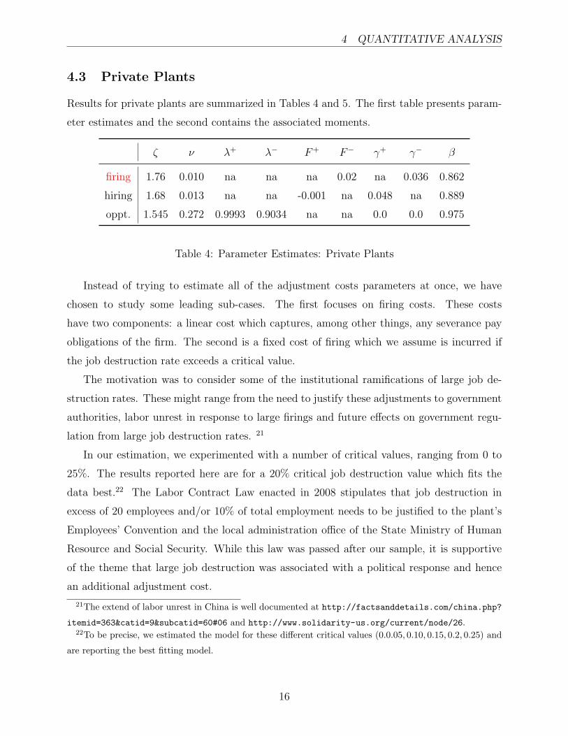
Results for private plants are summarized in Tables 4 and 5. The first table presents param-

eter estimates and the second contains the associated moments.

ζ ν λ+ λ− F+ F− γ+ γ− β

firing 1.76 0.010 na na na 0.02 na 0.036 0.862

hiring 1.68 0.013 na na -0.001 na 0.048 na 0.889

oppt. 1.545 0.272 0.9993 0.9034 na na 0.0 0.0 0.975

Table 4: Parameter Estimates: Private Plants

Instead of trying to estimate all of the adjustment costs parameters at once, we have

chosen to study some leading sub-cases. The first focuses on firing costs. These costs

have two components: a linear cost which captures, among other things, any severance pay

obligations of the firm. The second is a fixed cost of firing which we assume is incurred if

the job destruction rate exceeds a critical value.

The motivation was to consider some of the institutional ramifications of large job de-

struction rates. These might range from the need to justify these adjustments to government

authorities, labor unrest in response to large firings and future effects on government regu-

lation from large job destruction rates. 21

In our estimation, we experimented with a number of critical values, ranging from 0 to

25%. The results reported here are for a 20% critical job destruction value which fits the

data best.22 The Labor Contract Law enacted in 2008 stipulates that job destruction in

excess of 20 employees and/or 10% of total employment needs to be justified to the plant’s

Employees’ Convention and the local administration office of the State Ministry of Human

Resource and Social Security. While this law was passed after our sample, it is supportive

of the theme that large job destruction was associated with a political response and hence

an additional adjustment cost.

21The extend of labor unrest in China is well documented at http://factsanddetails.com/china.php?

itemid=363&catid=9&subcatid=60#06 and http://www.solidarity-us.org/current/node/26.22To be precise, we estimated the model for these different critical values (0.0.05, 0.10, 0.15, 0.2, 0.25) and

are reporting the best fitting model.

16


Looking first at firing costs, there is evidence of both fixed and linear firing costs. By

a normalization, the estimated fixed firing cost is 2% of steady state revenues. The linear

adjustment cost is estimated to be 0.036 which is about 0.04% of steady state revenue. From

Table 1, this cost is about 25,000 RMB per worker, a little less than two years of median

wages in the sample. Since the fixed cost only applies for job destruction in excess of 20 %,

the linear cost is important for obtaining inaction in adjustment since the adjustment cost

function is not differentiable at zero net employment growth. There is also a sizable cost of

adjusting as ζ = 1.43 but this cost is lower than that typically used in studies of US plants.23

Finally, the model allows for some quadratic adjustment cost but the estimate of ν is very

small.

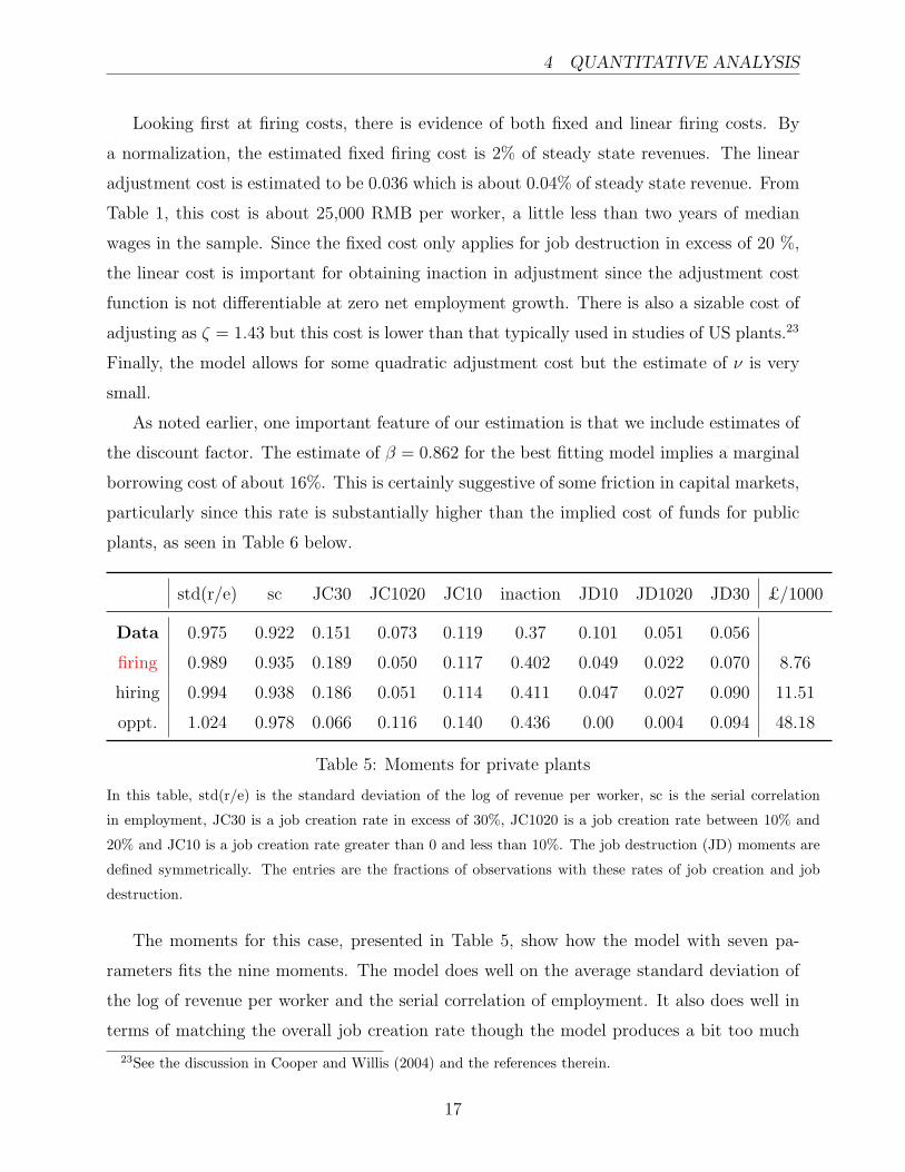
As noted earlier, one important feature of our estimation is that we include estimates of

the discount factor. The estimate of β = 0.862 for the best fitting model implies a marginal

borrowing cost of about 16%. This is certainly suggestive of some friction in capital markets,

particularly since this rate is substantially higher than the implied cost of funds for public

plants, as seen in Table 6 below.

std(r/e) sc JC30 JC1020 JC10 inaction JD10 JD1020 JD30 £/1000

Data 0.975 0.922 0.151 0.073 0.119 0.37 0.101 0.051 0.056

firing 0.989 0.935 0.189 0.050 0.117 0.402 0.049 0.022 0.070 8.76

hiring 0.994 0.938 0.186 0.051 0.114 0.411 0.047 0.027 0.090 11.51

oppt. 1.024 0.978 0.066 0.116 0.140 0.436 0.00 0.004 0.094 48.18

Table 5: Moments for private plants

In this table, std(r/e) is the standard deviation of the log of revenue per worker, sc is the serial correlation

in employment, JC30 is a job creation rate in excess of 30%, JC1020 is a job creation rate between 10% and

20% and JC10 is a job creation rate greater than 0 and less than 10%. The job destruction (JD) moments are

defined symmetrically. The entries are the fractions of observations with these rates of job creation and job

destruction.

The moments for this case, presented in Table 5, show how the model with seven pa-

rameters fits the nine moments. The model does well on the average standard deviation of

the log of revenue per worker and the serial correlation of employment. It also does well in

terms of matching the overall job creation rate though the model produces a bit too much

23See the discussion in Cooper and Willis (2004) and the references therein.

17


job creation in excess of 30%. The linear cost of firing produces inaction, a bit in excess of

the observed rate. The model struggles to match the intermediate levels of job destruction,

though it matches the tail of the job destruction distribution quite well.

The fit of the model, reported in the final column, is very far from zero. In a statistical

sense, the model does not match the moments. This is partly because we are estimating a

single model for all of manufacturing. Further, the moments are quite accurately measured

so that the variance/covariance matrix has very small elements. Consequently, the weighting

matrix used in the objective function has very large elements. All of the elements along the

diagonal of the weighting matrix have an order of magnitude equal to 6.

The hiring cost model is shown in the second row of Tables 4 and the third row of Table

5. In this case, there is a linear hiring cost of about the same magnitude of the linear firing

cost estimated in the first model. But there is no evidence of a fixed hiring cost.24 For this

model, we did not see any rationale for considering different job creation levels at which

the fixed hiring would apply. As in the firing cost model, the quadratic adjustment cost

is quite small. Compared to the firing cost model, there is a slightly smaller cost of hours

adjustment.

Looking at the moments for this case, the fit of the model with hiring costs is not as good

as the firing cost model. The relative standard deviation and serial correlation moments are

matched reasonable well. The model also matches the overall job creation and destruction

rates but misses on the composition, putting too much of the distribution in the tails relative

to the data.

The issue of distinguishing hiring from firing costs is not new. If there are costs of firing

workers, then a firm has a reduced incentive to hire workers. In effect, the firing cost appears

to be a hiring cost. In their estimation of a structural search model, Cooper, Haltiwanger,

and Willis (2007) find that many of the moments can be explained by a model with firing

costs and that neither specification can match all the moments of the employment growth

distribution.

The final specification focuses on the contribution of opportunity costs of adjustment,

rather than fixed costs. In this case, labor adjustment entails the shut-down of a plant for a

period of time represented by (1− λi) for i = +,−. As discussed in the data appendix, we

re-estimated the revenue functions for this model since the adjustment parameter interacts

24In fact, the point estimate indicates a slight fixed benefit for hiring.

18


with the flow of revenues. In this case we also allowed for a linear firing and hiring cost and

estimated β as well.

The results are shown in the row labeled “oppt.” in the two tables. The parameter

estimates again indicate a cost of varying hours and more of a quadratic adjustment cost

than the previous model. The main source of non-convexity in this case is in the opportunity

cost associated with job destruction. The estimated lost revenue is large: almost 10%. There

is no evidence of either linear hiring or firing costs in this specification. In this case, the

estimated β = 0.975, much higher than in the other specification.

As a consequence, for this specification the job destruction rates, shown in Table 5, are

all very tiny. Along that dimension, this model fails to match the data. The fit is not as

good as the firing cost model.

Overall, the best fitting model is one with linear and fixed firing costs. Importantly, the

non-convex adjustment cost applies when the job destruction rate exceeds 20%. And the

estimated discount factor is 0.862 for private plants.

4.3.1 Other Implications

There are some other properties of the estimated model with firing costs worth noting. While

these are not part of the formal estimation exercise, they indicate other dimensions along

which the model matches features of the data.

Returning to Table 3, we use the IV estimates to parameterize the private plant dynamic

optimization problem. At the estimated parameters, we simulated data and estimate using

OLS the relationship between revenue and the labor input and compare this against the OLS

estimate in Table 12. In the simulated data, the OLS estimation of the revenue function has

a curvature of 0.57, well above the value of α = 0.3198 used to parameterize this function.

The difference, of course, reflects the endogenous labor decision. The bias in the estimate is

not quite as large in the simulated data as in the actual data.

Our estimate does not utilize data on compensation. Yet the model has implications

for the cross sectional distributions of wages. These differences arise from the plant-specific

profitability shocks leading to differences in hours across plants and through the estimated

compensation function to differences in wages. The (time series) average of the coefficient

of variation of compensation, which equals the standard deviation of compensation divided

by the mean of compensation, is about 1.3 in the model. In the data, it is slightly over 1.0.

19


This difference between model and data may reflect excessive heterogeneity across plants in

the model relative to the data, less hours variation in the data relative to the model or less

sensitivity of compensation to hours variation in the data relative to the estimates.25

Finally, there is considerable employment inaction in the data which is replicated in the

model. One interesting question about the inaction is whether it is size dependent. In our

specification, the fixed cost of firing is proportional to the average revenue and so does not

vary with the size of a particular plant. That is, the fixed cost is not state dependent. This

contrasts with the opportunity cost model where the adjustment cost is state dependent and

is higher for larger plants. This suggests that looking at the pattern of inaction across plant

size might be informative about the nature of adjustment costs.

To do so, we looked at the correlation between size and inaction. In the data, the

correlation between inaction and size (measured as the number of workers) is -0.09. In the

simulated data this correlation is -0.0019. Thus the fixed firing cost model is replicating the

independence of inaction from size found in the data.

4.4 Public Plants

Tables 6 and 7 present results for public plants. As we did for the private plants, we consider

some leading specifications, indicated by the rows of these tables. The next section compares

the results for public and private plants.

The first case is firing costs. As with the private plants, the best fitting model had the

firing cost starting with a 20% job destruction rate. For that model, the cost of adjusting

hours is present but smaller than for the private model. The fixed firing cost and the linear

firing costs are modest. We estimated β = 0.9242 for the firing cost model. It does seem

that the profit maximizing motive is an effective way to model the choices of these plants.

The overall job creation rate matches the data well but the model does not produce the

burst of job creation found in the data. The model has about the same inaction as in the

data. As with job creation, the overall job destruction rate is close but the model does not

have the bursts of job destruction.

As was the case with the private plants, the other two leading specifications do not fit

the data as well. The opportunity cost model highlights firing costs and thus is unable to

25As we do not have data on hours variation, it is not possible to check these explanations directly.

20


match the pattern of job destruction found in the data.

The hiring cost model also does not fit the data quite as well as the firing cost specification.

Note that this specification estimates a positive cost of hiring rather than a fixed benefit

to hiring as discussed earlier as an alternative objective for public plants. This is evidence

against the “job creator” objective of SCEs.

Finally, we estimated the model allowing for a soft-budget constraint. As described

earlier, in this specification, the public plant receives a transfer from the government to cover

any losses. Of the adjustment cost cases with the soft-budget constraint, the opportunity

cost model was closest to the data and is reported in the tables. This is quite different from

the results without the soft budget constraint. The estimated model has only an opportunity

cost of firing workers. The estimate of β in this case was 0.915.

However, as seen in Table 7 adding in the soft-budget constraint did not improve the fit

of the model compared to the case of firing costs and no soft budget constraint. Thus we

conclude that the soft budget constraint is not influencing the labor demand decisions of

these public plants.

ζ ν λ+ λ− F+ F− γ+ γ− β

Trimmed public plants

firing 1.21 0.485 na na na 0.022 na 0.056 0.9242

hiring 1.327 1.069 na na 0.001 na 0.11 na 0.975

oppt. 1.629 1.70 1.0 0.813 na na 0.0 0.0063 0.9985

Trimmed public plants with sbc

oppt. 1.93 1.05 0.999 0.987 na na 0 0.008 0.993

Table 6: Parameter Estimates: Public Plants

4.5 Comparing Public and Private Plants

Given the large number of cases it is useful to highlight key findings. Here we focus on a

comparison of public and private plants.

For both public and private plants, the specification with firing costs fits the moments

best, with the fixed cost of firing occurring with job destruction rates in excess of 20%. Com-

21



Data 1.118 0.952 0.085 0.068 0.173 0.278 0.227 0.063 0.044

Trimmed Public plants

firing 1.084 0.992 0.003 0.078 0.215 0.331 0.271 0.083 0.000 2.806

hiring 1.034 0.993 0.001 0.0751 0.225 0.338 0.279 0.069 0.00 3.167

oppt. 1.166 0.967 0.045 0.127 0.197 0.393 0.00 0.024 0.065 7.110

Trimmed Public plants with sbc

oppt. 1.202 0.841 0.027 0.145 0.230 0.273 0.124 0.064 0.051 6.946

Table 7: Moments: Trimmed Public Plants

pared to private plants, public plants have lower costs of adjusting hours, higher quadratic

adjustment costs and higher linear adjustment costs.

Since one interpretation of the linear adjustment costs is severance payments, the larger

estimates of γ− for the public plants is consistent with the higher wages paid by these

plants. Returning to our discussion of the objectives of SCEs, we find some support for

the “employment stabilizing” objective, seen here as higher quadratic adjustment costs for

public plants.

Finally, estimating β improves the fit of the model slightly relative to the standard prac-

tice of assuming a discount factor. More importantly, we find that public plants discount

considerably less than the private plants. This is consistent with accounts of financial fric-

tions for private plants within China. Cull and Xu (2003) and Cull and Xu (2005), for

example, discusses the flow of (subsidized) funds to SCEs from public banks and the gov-

ernment. Among other things, they point out that the allocation of credit by state-owned

banks contains, in part, the bailout of SCEs. Hale and Long (2010) find that the ratio of

interest expense to debt is almost twice as high for private plants compared to SCEs.

4.6 Sectoral Results

Our estimates thus far pertain to all manufacturing plants. This approach constrains the

parameters to be the same across sectors. We now study a couple of specific sectors: autos

(and parts) as well as steel and iron.

Table 8 is comparable to Table 1 in terms of providing some basic statistics on the

22


(trimmed) public and private plants in the two sectors. Most of the plants in these sectors

are private. The public plants are considerably larger than the private ones. This is true in

terms of value added, revenues, employment and the capital stock. Public plants are more

capital intensive. The revenue per worker and revenue per capital measures of productivity

are all higher in the public plants. The difference in productivity is most evident in the

revenue per capital measure in steel and iron.

Table 9 provides IV estimates of the revenue function for these sectors. Clearly there are

differences across sectors in the curvature of the revenue functions and the persistence of the

shocks. For both private and public plants, the sectoral estimates of α are larger than for

total manufacturing.

The following two tables present estimate for the firing cost model by sector. For these

results, we estimated the model with firing costs, which was the best fitting model for all

sectors.

Some of the basic patterns from total manufacturing appear in the sectoral results as

well. The public plants have significantly larger quadratic adjustment costs and higher

linear adjustment costs. This is particularly true for the public steel and iron plants. Those

plants also have substantially larger fixed firing costs.

One interesting difference from the previous results is in the discount factors. For the

public auto plants, there is almost no discounting while the public steel and iron plants

discount more than the private plants. In the steel and iron sector, concern over excess

capacity has led the government to restrict credit to these plants and this may explain the

lower discount rate.26

In these two sectors, the discount factor for the private plants is much higher than it is

for overall manufacturing. It might be that the private plants in these sectors are parts of

firms with relatively easy access to capital markets.

As indicated in Table 11, the sectoral models fit better. This is both because the pa-

rameter estimates are sector specific. In addition, with a smaller number of observations,

the terms in the variance/covariance matrix are larger and thus the terms in the weighting

matrix are smaller.

26This policy is discussed in: http://industry.oursolo.net/data/steel-industry-iron-capacity/ and

http://www.robroad.com/light-industry/index.php/capacity-industry-million/.

23


Autos and Auto Parts Steel and Iron

All Public Private All Public Private

# plants 4,650 778 3,652 3,969 539 3,237

Value added 62,687 122,387 21,196 133,159 268,128 36,341

(524,559) (684,604) (60,372) (1,027,953) (1,024,121) (78,114)

Revenue 257,884 493,999 77,084 480,585 1,092,618 151,529

(2,078,417) (2,509,979) (230,453) (2,944,061) (3,548,125) (334,305)

Employment 336 537 177 534 1,110 168

(1,574) (808) (179) (3,406) (2,899) (207)

Capital 50,383 97,665 17,056 158,850 380,198 21,248

(365,652) (444,121) (47,459) (1,593,874) (1,432,630) (58,250)

Cap./Emp. 91 105 85 127 172 114

(158) (155) (153) (269) (509) (198)

VA/Emp. 127 128 120 235 234 229

(288) (252) (279) (509) (559) (507)

VA/Cap. 4.3 5.4 4 10.3 20.9 8.9

(43) (94) (22) (215) (543) (86)

Rev./Emp. 461 492 427 1,004 1,169 955

(958) (850) (919) (2791) (5838) (1940)

Rev./Cap. 15.1 16.1 14.7 43.6 78.4 38.8

(103) (173) (84) (854) (1942) (517)

Table 8: Types and Characteristics of Plants by Sector: 2005-2007

All monetary terms are in 1,000 RMB, deflated to 2005 level. The trimmed sample is

the public (private) sample excluding the upper and lower 2.5% tails by employment size.

Standard deviations are parenthesized.

24

5 CONCLUSION

α ρ

Autos and Auto Parts

private 0.4195 0.9162

public 0.5765 0.9412

Steel and Iron

private 0.3376 0.8557

public 0.6051 0.9227

Table 9: Sectoral Results from IV Revenue Function Estimation

ζ ν F− γ− β


private 1.26 0.049 0.005 0.040 0.968

public 1.12 0.27 0.001 0.060 0.999

Steel and Iron

private 1.86 0.0161 0.013 0.033 0.956

public 1.39 0.827 0.037 0.499 0.907

Table 10: Parameter Estimates by Sector

5 Conclusion

This paper estimates labor adjustment costs for private and public plants. For all of these

plants, we find evidence of adjustment costs in the form of fixed and linear firing costs along

with quadratic adjustment costs. These fixed firing costs apply when the job destruction

rate exceeds 20%. The quadratic adjustment costs for the trimmed sample of public plants

are larger than those for the private plants. Private plants discount the future more heavily

than do public plants.

Turning specifically to the objectives of the public plants, we see no evidence of soft-

budget constraints influencing the labor demand of public plants. Nor do we see evidence

of a positive benefit to hiring for these plants. Instead, we see support for public plants

acting to stabilize employment, as reflected by larger estimated quadratic adjustment cost

25

5 CONCLUSION



Private

Data 0.863 0.932 0.185 0.098 0.137 0.304 0.107 0.039 0.039

Sim. 0.759 0.963 0.085 0.076 0.147 0.370 0.097 0.062 0.041 0.442

Public

Data 1.012 0.967 0.084 0.104 0.201 0.231 0.206 0.061 0.031

Sim 0.999 0.981 0.055 0.103 0.185 0.256 0.146 0.102 0.032 0.038

Steel and Iron

Private

Data 0.943 0.933 0.173 0.075 0.107 0.361 0.098 0.050 0.054

Sim 0.960 0.910 0.197 0.067 0.094 0.354 0.054 0.045 0.079 0.136

Public

Data 1.154 0.982 0.094 0.0565 0.215 0.253 0.242 0.063 0.024

Sim 1.172 0.978 0.084 0.088 0.128 0.359 0.089 0.081 0.034 0.037

Table 11: Moments by Sector: Firing Cost Model

parameters for public plants.

This estimation exercises uses data prior to the introduction of worker protection regula-

tions in China. That intervention, in part, reflected concerns about hours variation and the

lack of severance pay to workers. One interpretation of the fixed firing costs for excessive job

destruction was a political one that may have been manifested in the recent regulations.27

Studying the impact of those new regulations on labor demand using our estimated model

is of considerable interest.

The results are also useful as inputs into an analysis of gains to reallocation. Given

our focus on private versus public plants, reallocation can occur within and across owner-

ship classes. We plan to use our model to study productivity implications of reallocation,

both in the present and in the earlier years of our sample. The theme of reallocation is

27See the discussion of the motivation for current regulations in http://www.carnegieendowment.

org/publications/?fa=view&id=22633 and http://www.law.com/jsp/law/international/

LawArticleIntl.jsp?id=1202430131324.

26

5 CONCLUSION

clearly important as well in considering the effects of the introduction of worker protection

regulations.

Appendix

This section discusses measurement of key variables and estimation of the revenue function

in (3) and section 4.1. “Revenue” in (3) refers to output price times quantity of output,

net of variable costs on inputs excluding labor. The data provide direct measures of output

in monetary terms, i.e. output price times quantity of output, which can be deflated to

base-year measures using the consumer price index.

Although the “revenue” (hereafter referred to as “net revenue”) in (3) is not directly

observed from the data, we can use the output price times quantity (hereafter referred to as

“gross revenue”) in the data to estimate the curvature of the net revenue function (α) and

back out the profitability shock. This approach is common in the dynamic factor demand

literature. The appendix of Cooper and Haltiwanger (2006) presents a detailed discussion

of the derivation and measurement issues in the context of a capital adjustment problem.

Assume a Cobb-Douglas production function is given by y = A(eh)αeKαK , where K

denotes inputs other than labor. These other inputs (hereafter referred to as capital) are

rented and incur no adjustment cost, with r being the rental rate. It is straightforward to

extend the production function with capital to a function with multiple variable factors.

Assume the plant faces an inverse demand function p = y−1/η. Here η is the price elasticity

of demand for the good. The net revenue function is given by

R(A, e, h,K) = [A(eh)αeKαK ]1−1η − rK, (14)

where the first term on the right-hand side is gross revenue. After optimization over K the

above equation yields

R(A, e, h,K) = (1− φ)[A(eh)αeKαK ]1−1η , (15)

where φ = αK(1− 1η). Note that the net revenue function and the gross revenue function are

the same up to a factor of 1 − φ. Substituting the first-order condition of the optimization

problem for K in equation (15) we obtain the net revenue function of the following form:

R(A, e, h) = A(eh)αe(1−1/η)

1−φ , (16)

27

5 CONCLUSION

where A = (1 − φ)A1

1−φ ( rφ)

φφ−1 . If the production technology is constant returns to scale,

then the curvature of net revenue on employment in equation (16) is exactly the same as

(12).

We estimate the revenue function via generalized method of moments (GMM). Specifi-

cally, we regress gross revenue from the data on total labor inputs (using total compensation

on labor as proxies for unobserved human capital differences in workers). Plant-level initial

wage and initial capital stock are used as instruments to control for some of the plant-level

heterogeneity. The total labor inputs is the number of workers (quality adjusted using the

initial wage) as hours worked is not observed. The lag of revenue is not used as an instrument

as current profitability is correlated with lagged profitability and thus lagged revenue.

The OLS and IV results are shown in Table 12. The curvature estimates are considerably

lower once we instrument for endogenous input variations.

α ρ

OLS

private 0.6695 0.8975

public 0.8272 0.9305

IV

private 0.3198 0.9082

public 0.4324 0.9513

Table 12: Results from Revenue Function Estimation

As China is a rapidly growing economy and our model is stationary, we include year

dummies as instruments to control aggregate profitability shocks. In the case of opportunity

costs, the estimation incorporates a dummy variable for employment adjustment to control

for the effects of disruption costs. In this case, we find α = 0.3968 for private plants and

α = 0.5593 for public plants, in comparison to the results in Table 3 for the fixed cost case.

We infer the profitability shock from the revenue function and the estimated coefficient

for α. The serial correlation (ρ) is obtained from an AR(1) process of the logarithm of

inferred profitability shock.

28

REFERENCES

References

Adda, J., and R. Cooper (2003): Dynamic Economics Quantitative Methods and Appli-

cations. MIT Press.

Bai, C., J. Lu, and Z. Tao (2006): “.The multitask theory of state enterprise reform:

empirical evidence from China.,” American Economic Review, 96, 353–57.

Bils, M. (1987): “The Cyclical Behavior of Marginal Cost and Price,” The American

Economic Review, 77(5), pp. 838–855.

Brandt, L., J. V. Biesebroeck, and Y. Zhang (2009): “Creative Accounting or Cre-

ative Destruction? Firm-Level Productivity Growth in Chinese Manufacturing,” NBER

Working Paper No. w15152.

Cooper, R., and J. Haltiwanger (2006): “On the Nature of the Capital Adjustment

Costs,” Review of Economic Studies, 73, 611–34.

Cooper, R., J. Haltiwanger, and J. Willis (2004): “Dynamics of Labor Demand:

Evidence from Plant-level Observations and Aggregate Implications,” NBER Working

Paper #10297.

(2007): “Search frictions: Matching aggregate and establishment observations,”

Journal of Monetary Economics, 54(Supplement 1), 56 – 78.

Cooper, R., and J. Willis (2004): “A Comment on the Economics of Labor Adjustment:

Mind the Gap,” American Economic Review, 94, 1223–1237.

Cull, R., and L. Xu (2003): “Who gets credit? The behavior of bureaucrats and state

banks in allocating credit to Chinese state-owned enterprises,” Journal of Development

Economics, 71(2), 533–559.

(2005): “Institutions, ownership, and finance: the determinants of profit reinvest-

ment among Chinese firms,” Journal of Financial Economics, 77(1), 117–146.

Gowrisankaran, G., and R. Town (1997): “Dynamic Equilibrium in the Hospital In-

dustry,” Journal of Economics & Management Strategy, 6(1), 45–74.

29

REFERENCES

Hale, G., and C. Long (2010): “What are the Sources of Financing of the Chinese

Firms?,” Hong Kong Institute for Monetary Research, Working Paper No. 19.

Hsieh, C.-T., and P. Klenow (2009): “Misallocation and Manufacturing TFP in China

and India,” Quarterly Journal of Economics, CXXIV(4), 1403–1448.

Lin, J., and Z. Li (2008): “Policy burden, privatization and soft budget constraint,”

Journal of Comparative Economics, 36(1), 90–102.

Sapienza, P. (2002): “What do State-Owned Firms Maximize? Evidence from Italian

Banks,” Available at http://ssrn.com/abstract=303381.

Song, M., K. Storesletten, and F. Zilibotti (2009): “Growing Like China,” CEPR

Discussion Paper No. DP7149.

30

Dynamic Labor Demand in China: Public and Private...

Documents

Transcript of Dynamic Labor Demand in China: Public and Private...