The Booking Window Evolution and its Impact on Hotel ... · reservation was made to a travel agent,...

The Booking Window Evolution and its Impact on Hotel Revenue Management

Forecasting

Timothy Dayton Webb

Thesis submitted to the faculty of the Virginia Polytechnic Institute and State University

in partial fulfillment of the requirements for the degree of

Doctor of Philosophy

In

Hospitality and Tourism Management

Zheng Xiang Co-Chair

Zvi Schwartz Co-Chair

Natalie Cherbaka

Manisha Singal

November 17th, 2017

Blacksburg, Virginia

Keywords: Revenue Management, Booking Behavior, Forecasting, OTAs


Forecasting

Timothy Dayton Webb

ABSTRACT

Travel booking behavior has changed substantially over the past two decades. The

emergence of new technology and online intermediaries has provided travelers with the

flexibility to book up until the date of stay. This has created a fast-paced, dynamic

booking environment that disrupts traditional revenue management strategies focused on

pricing and allocating rooms based on the time of purchase. The study explores the joint

effects of technology and the economy on booking window lead times. It also evaluates a

range of forecasting techniques and the importance of utilizing the booking curve for

forecasting in dynamic booking environments.

iii


Forecasting

Timothy Dayton Webb

GENERAL AUDIENCE ABSTRACT

Travel booking behavior has changed substantially over the past two decades. The

emergence of new technology and online intermediaries has provided travelers with the

flexibility to book up until the date of stay. This has created a fast-paced, dynamic

booking environment that disrupts traditional revenue management strategies focused on

pricing and allocating rooms based on the time of purchase. The study explores the joint

effects of technology and the economy on booking window lead times. It also evaluates a

range of forecasting techniques and the importance of utilizing the booking curve for

forecasting in dynamic booking environment.

iv

Table of Contents

Introduction ..........................................................................................................................1

Literature Review.................................................................................................................2

The Evolution of Travel Purchases ..................................................................................2

The Deal Seeking Culture & Time of Purchase ...............................................................3

Economic Indicators and Travel Purchases .....................................................................5

Travel Purchases Taken Together ....................................................................................6

Forecasting in Revenue Management ..............................................................................7

Forecasting in the Dynamic Booking Environment .........................................................8

New Forecasting Methods ................................................................................................9

Multi-Layer Perceptron Models .....................................................................................10

Research Question 1 ...................................................................................................11



Research Question 1 ..........................................................................................................14

Methodology ..................................................................................................................14

Data ................................................................................................................................14

Results ............................................................................................................................14


Methodology ..................................................................................................................16

Data ................................................................................................................................18

Results ............................................................................................................................20


Methodology ..................................................................................................................26

Data ................................................................................................................................26

Results ............................................................................................................................26

Conclusion .........................................................................................................................27

Limitations .........................................................................................................................28

Future Research .................................................................................................................29

References ..........................................................................................................................30

Appendix ............................................................................................................................36

Appendix A Cross Correlation Results ..........................................................................36

Appendix B Absolute Error Wilcoxon Test Results ......................................................37

v

List of Figures

Figure 1. Multi-Layer Perceptron: Network Architecture .................................................17

vi

List of Tables

Table 1. Average Quarterly Booking Window ..................................................................13

Table 2. Cross-Correlation Results ....................................................................................14

Table 3. Regression Results: DV - Quarterly Booking Window .......................................15

Table 4. Regression Results: DV – Log Quarterly Booking Window ...............................16

Table 5. West Coast Property 1 – Reservation Average Lead Time .................................19

Table 6. West Coast Property 2 – Reservation Average Lead Time .................................19

Table 7. North West Property 1 – Reservation Average Lead Time .................................19

Table 8. Mid-West Property 1 – Reservation Average Lead Time ...................................19

Table 9. Observations for Each Location ..........................................................................20

Table 10. West Coast Property 1 – Forecast Errors ...........................................................22

Table 11. West Coast Property 2 – Forecast Errors ...........................................................23

Table 12. North West Property 1 – Forecast Errors ...........................................................23

Table 13. Mid-West Property 1 – Forecast Errors .............................................................24

Table 14. MLP – Wilcoxon Hold Out Performance ..........................................................24

Table 15. Log Regression – Wilcoxon Hold Out Performance .........................................24

Table 16. Curve Similarity – Wilcoxon Hold Out Performance .......................................25

Table 17. MLP – Wilcoxon Booking Window Performance ............................................25

Table 18. Log Regression – Wilcoxon Booking Window Performance ...........................25

Table 19. Curve Similarity – Wilcoxon Booking Window Performance ..........................25

Table 20. T-Test Results ....................................................................................................27

1

Introduction

The emergence of revenue management (RM) over the last 30 years has created

substantial benefits for the hospitality industry in pricing and rate optimization. Revenue

management can be implemented in industries that have perishable products such as

hotels and airlines (Schwartz, 1998). These industries experience a constrained capacity

to be sold for a given duration (ex. flight or hotel night) and are unable to accumulate

inventory to be sold at a later date. Using revenue management optimization algorithms,

revenue managers can improve the profitability of hospitality companies by allocating

their inventory to the customers with the highest willingness to pay. This process is

typically conducted by forecasting demand, then opening and closing rate levels based on

the demand and the probability of selling a product (Phillips, 2005). Utilizing this

process, the hotel, airline and rental car companies are able to generate more revenue by

efficiently allocating their perishable inventory. The success of RM can be seen across

these industries with revenues increasing from $200-$500 million for airline companies

with revenues over $1 billion (Relihan, 1989). Similarly, hotel companies have increased

revenues from 2-5% from utilizing revenue management systems (Choi & Kimes, 2002).

Since its inception in the 1980’s, revenues have continued to improve as the

sophistication of the revenue management systems continues to evolve. Along with its

success, new challenges have emerged with the influence of technology. Prior to 2000,

booking reservations was largely dependent on information available from travel agents

who had access to global distribution systems (GDS). During this time, when a

reservation was made to a travel agent, the agent would enter the booking information

into the GDS which would communicate through a switch to a travel company’s central

reservation system (CRS) (Choi & Kimes, 2002; O’Connor & Frew, 2002; Thakran &

Verma, 2013). This information would then be communicated to the property

management system where inventory levels would be updated. At the time, the process

was relatively efficient. Travel agents bridged a key information gap regarding what

travel products were available and at what cost, instead of forcing the customer to

physically call various locations.

Given this structure, revenue management systems capitalized on a segmentation

scheme centered around the time of purchase. This was largely attributed to leisure

travelers booking well in advance due to the lack of information available, while business

travelers booked close to the date of travel due to the nature of business. For years,

revenue management systems leveraged price discrimination strategies by adjusting rates

upwards as the date of stay neared, considering that business travelers had a higher

willingness to pay. These adjustments in rate levels largely provided the revenue

increases for travel companies by selling the greatest amount of perishable inventory at

the most optimal price.

The recent changes in booking behavior due to technology have presented new

challenges for revenue management practices. It is now more difficult to predict who is

booking when and at what price, fundamentally changing the traditional segmentation

scheme. The study first investigates the causes of recent booking window shifts to

identify the drivers that have influenced change. In later chapters, revenue management

forecasting algorithms are compared to identify the most accurate models amidst

2

dynamic booking windows. Finally, these techniques are grouped into subclasses to

further identify which data types are most important for forecasting in dynamic booking

environments.

Literature Review

The Evolution of Technology and Travel Purchases

The emergence of the information age and an internet driven society changed the

way travel products were booked with online travel agents (OTAs). The first large scale

OTA was Expedia, developed by Microsoft in 1996, followed by Priceline in 1997

(Barthel & Perret, 2015). These outlets began selling holiday reservations online, but

quickly expanded to include all aspects of hospitality, incorporating everything from

flights and hotels to cruises and restaurants. Soon thereafter, several other sites emerged

such as Orbitz in June of 2001 and Kayak in 2004 (Empson, 2012; Thomas, 2016). The

success of these distribution channels is attributed to the fact that they provided

customers with a new and much improved resource for evaluating travel decisions. The

effects can be characterized in two distinct ways (O’Connor & Frew, 2002), the first is

that reservation information was now available in a timely and up to date manner in

which, a traveler could evaluate several different options at any time. Secondly, the

actual purchase could be conducted online. Although these changes seem relatively

simplistic, there impacts have changed the distribution of hospitality services forever.

Reservations could now be made on the go and the information regarding where to stay,

when, and at what price was not dependent on communicating with a travel agent or

property. The momentum for the new booking process has sustained as the uncertainty

associated with travel decisions is reduced. The distribution channels have assisted

travelers in minimizing the information gap between expectations and what a customer

may actually experience with reviews and recommendations.

This shift in consumer behavior has generated significant discussion within the

travel industry due to its shear dominance. For example, consider that in 2013, 45% of

all European travel revenue was conducted on OTA’s (Barthel & Perret, 2015). In the

first quarter of 2015, bookings through OTA’s increased 15% year over year, while

reservations made through hotel websites increased 7.1% (Mahmoud, 2015). Similarly,

over the same period, bookings made directly to the property (face-face or by phone)

dropped 8.4% and bookings through call centers dropped 6.1% (Mahmoud, 2015). In a

recent study conducted by Compete and funded by Expedia Media Solutions, it was

reported that customers visit travel sites approximately 38 times during the 45 days

leading up to a booking (Worgull, 2013). Even more revealing is that travelers visited

OTA sites 8 times during the week leading up to booking, with 1/3 of these visits

occurring on the day of (Worgull, 2013). The trends suggest that online booking will

only continue to grow, with OTA’s serving as one of the dominant resources for

travelers. The online booking environment is also technologically dynamic with the

recent emergence of mobile bookings from smart phones or tablets (Thakran & Verma,

2013). In 2014, 25% of leisure travelers booked with a smart phone up from 15% in the

prior year (Gasdia, 2015).

3

The shift in booking behavior has led researchers to begin considering the

implications for revenue management. The traditional purchase process is composed of 5

unique steps known as need arousal, information search, evaluation, purchase decision

and post-purchase feelings. However, for hospitality products, purchase and

consumption typically occur at different time periods. In addition, two components of

the purchase phase, price and availability are not stable over the purchase cycle

(Schwartz, 2006). Ultimately these factors can influence a customers’ willingness to pay

and decision of when to purchase.

To understand the decision process, Schwartz (2000) highlights the four options a

consumer can make when purchasing a hotel room, these include Book, Book and

Search, Search, and Other (select another product). The study by Schwartz (2006)

describes the interaction of these decisions with regards to price and utility, which

dictates the decision of the customer. These relationships create decision zones that are

derived by maximizing a customer’s utility with regards to the price, willingness to pay

and customer perceptions (Schwartz, 2006). The ultimate goal for researchers and

industry professionals is to develop strategies that influence the outlined factors to move

the zone switching points (Example: Book to Book and Search) in the decision process to

higher rate levels (Schwartz, 2006). Some of these strategies include increasing the

perception of a sellout or decreasing the perception of a discount, both of which can

increase the book and book and search zone switching price points and capture more

bookings.

Further complicating the purchase process is the effects of time on these decision

zones. Customer expectations and subjective assessments of future dates cannot be

assumed to be stationary as the date of stay gets closer (Schwartz, 2008). For instance, as

time progresses the number of searches a customer can conduct diminishes; similarly, the

perceptions regarding the chance of a sell out or price change are not static. It has been

shown that time dependency can impact the booking decision even if the rate does not

change (Schwartz, 2008). These findings highlight the effect that time dependency can

have on booking decisions, and further stresses the complex predicament of the advanced

purchasing process, which plays an integral role in decision making of revenue managers

and revenue management systems.

The Deal Seeking Culture & Time of Purchase

It is evident that the traditional purchase process that was limited in the past has

now evolved into a dynamic environment that has serious implications for revenue

management with regards to when a purchase is made. The emergence of the internet

provides several new factors (price changes, sell out risk etc.) that may influence the

purchase decision. Given the dynamic nature, travelers may continuously evaluate these

factors as they may change up until the actual date of stay. As the internet has become

more prevalent, it has created consumer search behaviors that involve adaptive search

patterns, learning elements and expectations updating (Schwartz, 2008; Worgull, 2013).

Coinciding with the change in when travelers choose to book, is the price that customers

are willing to pay. What has arisen due to the internet has largely been considered a

“deal seeking environment”. The reasons for development of this deal seeking culture

are outlined by O’Connor (2002). He states three key underpinnings, the first is that

4

internet retailers (such as Amazon) compete with traditional outlets largely based on

price. Secondly, consumers are aware of the lower distribution costs online, from

eliminating the middle man. Finally, last minute promotions pushed by hospitality

companies are used to sell distressed inventory, which has generated traveler associations

with cheaper prices (O’Connor, 2002; Decko, 2004). Further adding to the feasibility of

the deal seeking environment is the decrease in search costs which has made price

shopping easier (Jang, 2005; Sahay, 2007). Finally, the deal seeking culture was

confirmed by Yesawich et al. (2000) in their survey “2000 National Leisure and Travel

Monitor” in which it was reported that almost 6 in 10 travelers search for the “lowest

possible rates”.

A more scientific argument for the development of the deal seeking culture has

been presented by Schwartz & Chen (2012). They argue that the purchase decision is

fueled by both utilitarian and hedonic motivations. In the traditional booking structure,

once a consumer decides to take a trip, the utilitarian motivations describing the need to

book the reservation dominates the purchase decision. A traveler selects a destination

and then selects a product that derives the highest benefit (utility) from the booking.

However, with the emergence of online information, hedonic motivations may enter the

purchase decision. In this instance, travelers know that prices and availability change

over time. The ease of checking rates creates a purchase process that travelers enjoy.

Ultimately, these customers generate additional utility from deal seeking in the online

environment in hopes of finding a cheaper rate. The investigated relationships show that

the impacts of revenue management strategies, such as sell outs or paying a higher rate,

must have a large enough impact on the purchaser to generate a booking closer to the

traditional booking time. If the perceived risk is not high enough, consumers will

continue to search for a better deal to obtain the enjoyment from the possibility of finding

a cheaper rate.

Overall, the emergence of these online intermediaries has created significant

benefits for the traveling consumer through its reduction in the information gap and

ability to make travel decisions, however, it has also had substantial implications for

revenue management. The first is with regards to the deal seeking culture in that travel

products such as hotels may be viewed as a commodity rather than a brand or specialized

product (Carroll & Siguaw, 2003). This makes pricing particularly more difficult as

differentiation may not be a way to maximize revenues. The second is that the decrease

in search costs and deal seeking culture has shifted the booking window (Dacko, 2004;

Mayock, 2011; Lee, 2013). In other words, the availability of travel prices and

information has altered when consumers book, detrimentally impacting the traditional

revenue management structure and segmentation scheme (Schwartz, 2006). Recall that

prior to OTA’s and internet bookings, leisure travelers tended to book well in advance,

while in today’s internet economy these travelers have the flexibility to book up until the

date of stay. This has generated significant problems since the accumulation of bookings

occur in a different fashion than they have historically and provide less information for

revenue managers and algorithms to operate efficiently. Decisions such as when to open

or close rate levels, or which pricing levers to pull is inherently more difficult as

inventory may be categorized as distressed earlier. These price changes ultimately

influence the customers’ willingness to book (Chen & Schwartz, 2008).

To highlight the relationship between time of purchase and deal seeking,

5

experimental research has shown that the propensity to book increased as the date of stay

drew near, however lower expected future rates decreased the probability of booking.

Therefore, although consumers have a higher need to book as the date of stay nears, they

are also likely to wait if they perceive the rates to be lower (Chen & Schwartz, 2013).

These results support the hedonic motivations suggested by Schwartz and Chen (2012)

and this effect has also been investigated by Toh et al. (2011). In his study, 13 properties

were tracked daily for quoted rates on the hotels website, Expedia and Orbitz. The

results of the study show that the quoted rate in the first 14 weeks of the booking window

were higher than the rate quoted during the last 3 weeks of the window. The authors

suggest this could be due to the shortened booking window. In the study, an interview

with a hotel employee stated that “It used to be a couple weeks when (late-booking

customers) rushed in. Now it’s three days. We’re not sure if it’s due to the recession the

internet or both.” Further evidence of the “deal seeking” culture and shrunken booking

window is discussed by Granados et al (2012) who show that consumer demand for

airline tickets is more elastic via online channels than offline channels. This is largely

attributed to the fact that leisure travelers are more likely to use these channels and are

more price sensitive (Granados et al, 2012).

Economic Indicators and Travel Purchases

Although the internet has provided travelers with the ability to book later and

search for deals, it does not guarantee that all of these travelers are deal seekers or choose

to wait. Several external factors may have conflicting impacts on the booking process.

As the quote from Toh (2011) indicates, the economic situation plays a pivotal role in

when consumers book and is also likely to affect the price and duration of stay (Legre,

2004; Toh, 2011). This is because travel and tourism is largely considered a luxury

product (Crouch, 1994; Smeral 2009). In other words, customers will forgo vacations for

necessary products such as food and clothing. Therefore, purchases of these products

tend to vary based on the state of the economic climate, with high responses to changes in

income, unemployment levels, and relative prices of goods, among others (Legre, 2004;

Smeral, 1988; Smeral, 2009). When looking at income levels specifically Legre (2004)

reports that the propensity to travel increases as income levels increase. However, the

effects of income elasticity on travel for lower income individuals is far greater than for

those with higher incomes (Legre, 2004). These findings suggest that economic factors

such as income and unemployment can have substantial effects on travel, influencing

when a consumer books as well as at what price and duration.

How each of these factors influences occupancy rates is discussed by Choi

(2003). In the study, an auto correlation function is used to create cross correlogram

plots between economic indicators and gross hotel commerce. Although several

indicators were identified, notable leading indicators of hotel revenues were CPI for

motor fuels (lag -4), GDP of Service (lag -2) and the hotel stock index (lag -2).

Coincident indicators of note included GDP, hotel occupancy percentage, consumer

confidence, and consumer expenditures in the service industry. Finally, lagging

indicators include GNP (lag 1), total employment (lag 1) and the unemployment rate (lag

2). These factors were used to build composite indices to forecast hotel commerce and

6

may be useful in determining not only how much may be spent on travel but also when

bookings occur.

Overall, the relationships between economic indicators and the travel industry are

well documented, it is important to note that not all properties are impacted the same.

Ismail et al. (2002) show that a hotels segment and location respond differently to

changes in the market. Their results show that high priced segments were most volatile

while low priced segments were least volatile in terms of RevPAR and the market. From

a location perspective, urban properties have a strong response to market changes while

airports and highway hotels were least affected (Ismail et al, 2002). These results are

largely attributed to the theory of trade up and trade down effects. Travelers tend to trade

up (to higher segments) when the economy is good but trade down to lower priced

options when the economy is bad (Ismail et al., 2002; Jones, 2005). The volatility of high

priced segments is because there isn’t any trade down gain because they are the top

segment. Similarly, mid-priced segments may add trade down customers from luxury

segments when the economy is bad. These findings support the fact that business

travelers and high income travelers are least effected by the economy while lower income

leisure travelers are most impacted.

Travel Purchases Taken Together

Ultimately, there are several compounding factors that influence travel booking

decisions today. In one domain, there are the impacts of technology which has provided

increased flexibility in the way consumers book, when they book and at what price. In

the second domain are the economic effects that are impacting the ability of consumers to

take a trip and similarly impacting when they book and at what price and duration. Over

the past few years, reports have shown conflicting arguments with regards to the shift in

the booking window. At times reports have suggested the booking window was

shrinking as Omni hotels reported that the average lead times for large meetings dropped

by 200 days between 2009 and 2011 (Mayock, 2011). A report from Travel Click (2012)

reviewed reservations data for 25 North American markets from August 2012 – July

2013. Their report showed committed occupancy (advanced reservations) was up 3.5%

for group travelers and 4.4% for leisure travelers, with an overall ADR increase of 4.1%

(Travel Click 2012). In a similar report, Manley (2016) cites that Travelclick transient

bookings were down -1.9% while average daily rate is up 2.1% (Manley, 2016).

Interestingly, group bookings were both up in committed occupancy and ADR over the

same period (April 2016-March 2017). In another article, Denihan Hospitality EVP Tom

Botts stated that the average booking was conducted 39 days in advance up from 35 the

previous year (Worgull, 2013). These reports suggest that the recent lengthening of the

booking window is due to an improved economy (Worgull, 2013). As Tim Hart, the

Executive Vice President for Research and Development at Travel Click states “Business

and leisure travelers are booking further in advance, no longer holding out until the last

minute (Travel Click 2012).”

The impact of the internet on revenue management cannot be understated as its’

potential impacts on forecasting, pricing and booking limits are critical to optimization

algorithms. It also seems evident that the change in booking behavior falls particularly

on the leisure travel segment as business travelers are likely to be booking within the

7

same window while leisure travelers have the ability to book at their own discretion. The

evolving dynamic of technology and purchasing power within the economy further

complicates the accuracy of the forecasting process. Forecasts within the hotel industry

are typically conducted for several factors including occupancy by rate class, length of

stay, walk-ins and no shows, among others. The more accurate the forecasts that feed the

revenue management systems, the better revenue managers and systems can make

decisions. This highlights the need for research to be continually conducted to enhance

the forecasting tool kit, attempt to discover the most accurate methods and to find

methods that are best suited and adaptive to these dynamic booking environments.

Forecasting in Revenue Management

To produce forecasts, the data readily available to a hotel property includes

historical booking information, current booking information and additional information

(Schwartz et al, 2016). The historical data is comprised of bookings that have occurred

on similar days in the past. This includes booking information for the same day year over

year. The current booking data is comprised of the reservations on hand for a date of stay

in the future, while additional information contains outlier days not typically observed.

These three types of information are then used to produce a forecast by leveraging a

variety of techniques that fall under one of three subclasses (Weatherford & Kimes,

2003). The first subclass utilizes the historical data and involves a time series approach.

The inclination behind this approach is that past observations will likely repeat due to the

seasonality involved with travel. The second subclass is with regards to the current data.

As bookings accumulate for a particular date of stay, the goal is to extrapolate the current

bookings on hand to determine how many additional rooms or reservations will be picked

up. The final subclass includes the current industry standard of combining the historical

and current data models together to produce a final forecast (Weatherford & Kimes,

2003). When the date of stay is far in advance (greater than 90 days) the historical

information tends to receive a higher weight as reservations have yet to accumulate.

However, as the date of stay approaches, bookings begin to occur more frequently and

the current data technique begins to receive more weight. This is where the ability to

yield rate levels becomes strategically important in the optimization algorithms as

booking limits are opened and closed based on the bookings and forecasted demand

(Chen & Kachani 2007; Phillips, 2005).

Several studies have attempted to determine which forecasting techniques are the

most accurate and robust for forecasting in revenue management. The first major study

conducted by Weatherford and Kimes (2003) tested seven different models on a variety

of hotels to predict room nights, as well as forecasts by rate class and length of stay. The

historical models tested included exponential smoothing, moving average and Holt-

Winters double exponential smoothing. The current data models included linear

regression, log-linear regression, additive pick-up and multiplicative pick-up. The study

tested these models on two separate data sets from hotel properties owned by Choice

Hotels and Marriot. Results of their study show that exponential smoothing was the most

accurate using MAE, while additive pickup was the most accurate using MAPE

(Weatherford & Kimes, 2003). The worst performing methods were log linear and

multiplicative pick-up methods. In a similar study conducted by Chen and Kachani

8

(2007) the exponential smoothing, classical pick-up, advanced pick-up, linear regression

and vector autoregressive (VAR) methods were tested with a variety of estimation and

hold out sample sizes. Their results show that regression was the worst method while a

combined version of the exponential smoothing and advanced pick-up performed well

(Chen & Kachani, 2007).

Researchers have also tested several novel ideas outside of the traditional time

series and extrapolation methods to improve accuracy, particularly in the face of the

dynamic booking windows. To account for when consumers are booking, researchers

have attempted to add consumer pulse data to traditional time series models (Pan et al

2012; Yang et al 2013). These methods include visits to travel websites and travel search

queries as additional explanatory variables in ARIMAX models. Their results show that

consumer data regarding travel planning can significantly improve the accuracy of

forecasts using the ARIMAX model over the traditional ARIMA model (Pan et al 2012;

Yang et al 2013). Researchers have also begun to add additional information to the

forecasting models to improve accuracy within markets. Schwartz et al. (2016) suggest

using a combination of several properties forecasts to determine an optimal forecast. In

this instance, each property makes a forecast and would then share that forecast with

others in the properties competitive set. The benefits lie in the fact that each property has

different information, market knowledge and modeling techniques that could be

advantageous to the others. These properties then use weighted combinations of the

competitive set to obtain a more optimal forecast. The results show that the combination

improves forecasting accuracy for hotels that have poor forecasts on their own or have

occupancy rates that are highly correlated within the market (Schwartz et al. 2016).

Forecasting in the Dynamic Booking Environment

The challenge surrounding forecasting with dynamic booking windows is most

evident with regards to current data forecasting techniques. Traditional pick-up methods

that are not frequently updated due to changes in consumer behavior may be problematic

considering that reservation pickup rates may change over time (Webb, 2016). As Tim

Hart, Executive Vice President, Research and Development at TravelClick stated in a

recent news article “Business and leisure travelers are booking further in advance, no

longer holding out until the last minute. For hoteliers, this means that it is important to

account for this shift in the booking window in their forecasting, relying less on

comparisons to last year’s booking pace and more on recent booking pace trends.” If

technology or the economy “shrinks” the booking window, adding the historical average

pickup may not be an accurate approach and inventory may be categorized as distressed

earlier; similarly, the reverse is also practical.

Interestingly, the study by Tse and Poon (2015) reveal that hotel industry

professionals tend to focus on future pickups from a fixed point in time, ignoring how

reservations accumulate. In their article, industry professionals state that “pickup rates at

different times are different and thus the booking data in early days or weeks bear no

relevance in forecasting.” This argument is particularly problematic in the face of

dynamic booking windows as the shift in reservation lead time can greatly alter the

pickups forecasted for future room nights. Tse and Poon (2015) correctly indicate that

forecasting techniques leveraging only future reservation pickups are utilizing an

9

approach that exhibits the Markov property in mathematics. The Markov property

indicates that future behavior of a process is not altered by the additional information of

past behavior (Lee 1990, Tse and Poon, 2015). For forecasting in revenue management,

this would imply that future bookings are independent from the current bookings on hand

and how these reservations accumulate.

Forecasting in dynamic booking environments requires an understanding of what

is dictating changes in the booking window and how to identify when these changes are

occurring. Tse and Poon (2015) argue that the lead time for reservations will vary from

period to period depending on several macro and micro factors (Tse and Poon, 2015).

Specifically, macro factors related to the economy (unemployment, exchange rates, GDP)

may impact booking behavior, while micro factors such as advertising and price

promotions may also impact pickup rates. Therefore, Tse and Poon (2015) state that

bookings on hand are a good indicator and reflection of all macro and micro factors that

affect room occupancy and may carry through the entire booking period. This argument

would suggest that the accumulation of the booking curve is critical to forecasting in

dynamic booking windows.

Models have been investigated that may improve accuracy within these

conditions. Schwartz and Hiemstra (1997) attempted to improve booking curve

extrapolation by proposing a booking curves similarity match technique. In their study,

they compare current booking curves (incomplete information) to past complete booking

curves to identify dates of stay with similar pick-up. This method uses a distances metric

every 10 days to compare similarities between curves. Once the similar curves are

identified, they are combined to estimate the final number of bookings. This technique

outperformed the competing techniques (autoregressive and higher order polynomials)

with an average reduction in MAPE of 5.2% (Schwartz & Hiemstra, 1997).

In another approach, Tse and Poon (2015) tested the effectiveness of fitting a

variety of polynomials to the booking curves at varying horizons. As the horizon moves

from one month out to two weeks out, the method becomes increasingly accurate and

demonstrates the potential success of using a second order polynomial on the booking

curve rather than simple linear regression. Specifically, their study shows that trends and

patterns in the data due to changes in booking lead times can be very useful for

forecasting.

Ultimately, both authors argue that the accumulation of reservations is an

important attribute for the extrapolation that should be leveraged. Other techniques of

extrapolation, such as additive pick-up assume that previous reservation pick-ups are

independent of future reservations. Both methods may help combat the dynamic booking

patterns as the booking curves technique may map to previous booking curves under

similar conditions (economic, technological, or other causes), while the higher order

polynomial regression also accounts for how reservations accumulate.

New Forecasting Methods

As technology and computational power has improved over recent years, the

techniques for forecasting have been refined and advanced. The most notable of these has

been the emergence of neural networks. Neural networks have been used heavily in

forecasting, classification and pattern recognition problems (Garson, 2014; Vellido et al.

10

1999; Weatherford, 2003). The technique was inspired by neuroscience to imitate a

process that is like the human brain (Guthikonda, 2005; Zhang et al. 1998). Within the

brain, neurons are connected and pass signals back and forth to communicate information

for reaction. Generally speaking, a neural network attempts to imitate this process by

creating linkages between inputs (predictors) and outputs (forecasts) (Garson, 2014;

Hyndman, 2014). In a typical structure input vectors (variables) are introduced to the

network. These inputs are connected by arc weights to hidden or output layers (Garson,

2014; Zhang, 1998;). The models are data driven techniques that learn from examples

and can capture subtle or unknown relationships between the input and output variables

(Zhang, 1998). The models also provide several advantages over traditional techniques

in that they are self-adaptive, non-parametric and require few a priori assumptions

(Garson, 2014; Zhang, 1998). In addition, they can capture any functional form and

incorporate nonlinear relationships which provides significant advantages over traditional

time series models (linear processes) (Vellido et al., 1999; Zhang et al., 1998).

Although several benefits of neural networks exist, there are also a few

drawbacks. The first is that it is difficult to establish casual relationships between inputs

and outputs (Garson, 2014). This is largely due to the structure of the network as the

relationship of the predictor variables to the dependent variable is obscured by the

indirect and iterative nature of the algorithms (Garson, 2014). Depending on the number

of layers within a network, several weights and intermediate relationships may exist

which make causal inferences difficult. Instead, the networks are best suited for

processes that require high predictive power without justification as to which variable is

deriving the solution. A second drawback is the issue of over-fitting as data driven

methods can be unstable across samples so it is important to cross validate. This process

requires one data set to fit the model and another to test for stability (Garson, 2014). It is

also important to note that the process is largely data driven and somewhat random so

several training iterations is recommended (Hyndman, 2014). Overall, the use of neural

networks for research problems has gained increased recognition over recent years due to

the flexibility the models provide. The models are particularly useful for forecasting

where accuracy is of upmost importance in comparison to casual influence regarding

which variables are included.

Multi-Layer Perceptron Models

Several neural networks have been derived to solve a variety of problems. One of

the most common neural networks is the multi-layer perceptron model which is typically

used for forecasting. This model is a feed-forward neural network where inputs are

introduced to the model and pass information to hidden layers. The hidden layer

communicates information forward to future layers until the output layer is reached

(Correa et al. 2012, Garson, 2014; Hyndman, 2014). In the estimation process the back-

propagation technique is used in which the error in the output layer is fed back to earlier

layers to update nodes and optimize a prediction (Correa et al. 2012; Garson, 2014); this

process is conducted after each iteration and is a gradient steepest descent method. The

typical estimation process is supervised, which means inputs and outputs are known in

advance and several iterations of training are used to estimate the model. The estimation

process continues until the error is minimized or reaches a predetermined constant. The

11

iterations are conducted several times to reduce randomness and the network weights are

averaged together after all the iterations. The estimated model is then tested on hold out

samples to ensure accuracy and reliability.

The extent of MLP applications is vast and has been leveraged by both

researchers and practitioners in many fields. Within the business domain, these models

have been used in the areas of accounting, finance and marketing (Vellido, 1999). From

the hospitality and tourism perspective, the techniques have gained some popularity in

recent years, particularly in forecasting for tourism, finance and revenue management.

Uysal and Roubi (1999) use a multi-layer perceptron model to forecast Canadian tourism

expenditures in the U.S. (Uysal et al. 1999). In another application, MLP’s were used to

predict occupancy rates for the Hong Kong hotel industry, as well as Japanese visitors to

Hong Kong (Law, 1998; Law, 1999). All three papers show the ability of neural

networks to outperform multivariate regression models and cite that this is likely due to

unobserved relationships between the variables. The MLP techniques have also been

used to forecast bankruptcy of hotel and restaurant firms with mixed success over the

traditional logistic regression techniques (Kim, 2011; Park et al. 2012; Youn et al. 2010a.

Youn et al. 2010b.).

Within the revenue management domain, researchers have utilized multi-layer

perceptron models to predict demand for airline products. Weatherford et al. (2003)

constructed a single layer feed forward neural network to predict the number of

reservations for airline flights. The single layer neural network is the most basic

architecture and his results show that the network was more accurate than traditional

smoothing and regression techniques (Weatherford, 2003). In addition to performance,

the error measures had more consistency between the estimation and hold out samples.

This result coupled with the idea that only the most basic structure was utilized would

suggest that further improvement could be obtained and may provide a superior method

for this type of forecasting. In the revenue management transportation field, Tasi et al

(2009) used a variety of neural networks to predict railway passenger demand (Tasi et al.

2009). Research suggests that like other disciplines the MLP technique has begun to gain

further popularity for forecasting in the field of hospitality and tourism, and has shown

potential within the field of revenue management.

Research Question 1

The reviewed literature and anecdotal observations suggest that the booking

window is fluctuating over time. However, academic research has lacked in determining

how technological changes in the booking process and the economic consumption

climate have jointly impacted booking behaviors, particularly over an extended period of

time. It may be that in general, technology has shrunk the booking window with brief

swings up and down due to the economy. Similarly, the change in technology may have

allowed consumers to book earlier but they were only doing so due to the economic crisis

in recent years. Understanding where the shifts in booking lead times are derived is

critical for revenue management operations as forecasting and prices are largely adjusted

based on the accumulation of reservations.

12

Research Question 1: To what effect has technological change and changes in the

economy had on booking window lead times?

Research Question 2

The fluctuation in booking window patterns presents significant implications for

forecasting in revenue management. As the booking window changes, it is important to

realize that it causes changes in the underlying data structure due to when reservations are

observed. These changes inherently impact the accuracy of techniques and are likely to

diminish the efficiency of forecasting methods if model parameters aren’t updated

accordingly. This is particularly true in current data techniques which are dependent on

reservation pickups at various points in time (Webb, 2016). The issue can have

detrimental impacts on revenues considering the key decisions such as what rate levels to

open and close or what distribution channels to use are based on these forecasts. Lee

(1990) has determined that a 10 percent improvement in forecasting accuracy can

contribute up to a 3% improvement in revenues for the airline industry (Lee, 1990).

Similarly, other studies have cited estimates that a 20% reduction in forecast error could

increase revenues by 1% (cited in Koupriouchina et al, 2014). These results suggest the

importance for continued research for forecasting within revenue management,

particularly in the face of dynamic booking windows. Neural networks may provide

increased forecast accuracy within hotel revenue management over an extended period;

with data sets that contain shifts in the booking window.

Research Question 2: Can neural networks provide more accurate forecasts than

traditional techniques, particularly with data containing booking window fluctuations?

Research Question 3

As the booking windows fluctuates, the accuracy of a current data techniques is

likely to diminish. Previous investigations tend to be limited in their analysis regarding

the robustness of techniques over time, when considering that these studies tend to utilize

less than two years of data. These smaller samples are unlikely to exhibit significant

shifts in reservation lead time and may be unsuitable to identify appropriate techniques to

be used for an extended period. Specifically, it is important to understand if utilizing the

accumulation of reservations in the forecasting algorithm provides a more robust model

than techniques that ignore this information in the face of dynamic booking windows.

Research Question 3: Do forecasting techniques that utilize the accumulation of

reservations in model estimation prove to be more robust as the booking window

fluctuates?

13

Research Question 1

Methodology

To assess the impacts of technology and the economy on booking window

fluctuations, the variables are first entered into an autocorrelation function (ACF) to

assess their relationship with the booking window observations. The ACF reveals

lagging or leading relationships between the independent and dependent variables and is

similar to Choi (2003). The strongest identified relationships will be utilized to model

booking window fluctuations. Sequentially, multivariate regression is used to measure

the effects of the economy and technology on booking window fluctuations. The

dependent variable is defined as the quarterly average booking window lead time, while

the independent variables are the quarterly economic and technological lead or lag

variables identified in the ACF. To account for differences in booking windows during

different time periods and across properties, indicator variables were assigned for each

location (P1-P14, p15 as reference) and quarter of year (Q1-Q3, Q4 as reference).

Formally

Data

Booking window fluctuations are most likely due to changes in the booking

behavior of the leisure segment who have more flexibility in travel plans. For this

reason, data was obtained from 15 properties located in and around National Parks in the

United States. These properties include locations around the entire continental US

including the Northeast, Mid-Atlantic, Northwest, Midwest and Southwest regions. The

average lead time for room nights at each property were obtained by quarter with the

earliest and latest time periods recorded in Table 1. The range of the quarterly average

booking windows are also provided for the given time periods.

Table 1. - Average Quarterly Booking Window

Property Region

Earliest

Quarter

Latest

Quarter

Minimum

QTR BW

Maximum

QTR BW

Average

QTR BW

1 West Coast Q2 2013 Q3 2016 97 185 167

2 Mid Atlantic Q3 2013 Q4 2016 32 97 48

3 North West Q1 2014 Q4 2016 23 52 80

4 North East Q1 2011 Q4 2016 18 67 44

5 West Coast Q1 2014 Q4 2016 15 103 67

6 North West Q1 2013 Q4 2016 31 77 52

7 North West Q1 2013 Q3 2015 20 65 45

8 North West Q1 2013 Q4 2016 20 117 57

14

9 Mid Atlantic Q3 2013 Q4 2016 13 45 29

10 North East Q1 2014 Q4 2016 21 69 51

11 Mid Atlantic Q3 2013 Q4 2016 18 71 44

12 West Coast Q1 2011 Q4 2016 26 94 65

13 Mid-West Q1 2009 Q4 2016 21 67 43

14 West Coast Q1 2011 Q4 2016 22 137 78

15 North West Q2 2013 Q3 2016 32 93 70

To estimate the impact of technology, the number of reservations made online

were taken as a percentage of total reservations. Specifically, all reservations made

through internet channels (property website, OTA’s) were taken as a percentage of all

reservations for the given quarter of stay. The economic variables were downloaded

from the United States Bureau of Labor Statistics and the United States Bureau of

Economic Analysis. From the Bureau of Labor Statistics, the Consumer Price Index,

Employment Level and Unemployment Level were recorded in monthly increments.

These metrics were averaged together to create quarterly metrics for each time period.

The United States Quarterly Gross Domestic Product (GDP) was recorded from the

Bureau of Economic Analysis. The data range spanned from the first quarter of 2000

until the first quarter of 2017.

To determine whether the economic variables have leading, lagging or coincident

impacts on the booking window, SAS 9.4 was used to run cross correlations between the

economic series and the average quarterly booking window. Three properties that had

the longest time series (2009, 2011 – 2016) were used to determine which variables were

leading or lagging with comparisons running 2 years (8 quarters). The results of the cross

correlations revealed the strongest relationships between the independent and dependent

variable in Table 2 to be included in the model. Similar to the study conducted by Choi

(2003), GDP was identified as a coincident indicator while Total Employment and

Unemployment were found to be lagging indicators. Results of the cross-correlation

analysis are provided in the Appendix.

Table 2. – Cross-Correlation Results

Economic

Variable

CCF - Identified

Lag

CPI 4 Quarters / 1

Year

Employment 1 Quarter

Unemployment 2 Quarters

GDP None/Coincident

Results

The results of the models are reported in Table 3. In each model, one economic

indicator was paired with the percent of bookings made online for the given quarter.

Several iterations of the model were run, however strong multicollinearity between the

15

economic indicators required that only one economic variable be included to avoid biased

parameter estimates. The results show that the percentage of online bookings did not

have a significant effect on booking window lead times. In other words, technology is

not driving the booking window shifts.

Interestingly, in all models the economic variables have a significant positive

relationship on booking window lead times. The results would suggest that as the

economy improves the booking windows expand and travelers tend to book further in

advance. Similarly, as the economy contracts booking windows will shorten. This can

likely be attributed to the fact that during strong economic times, increased financial

security allows travelers to book further in advance with the confidence that they can

afford the trip. To test for robustness, the models were re-estimated using the log of

average booking window lead times to enhance normality of the dependent variable. The

outcome of these models, provided in Table 4, show the same relationships that were

obtained using the untransformed dependent variable. The results further validate the

relationship of technological and economic variables on booking window lead times at

these locations.

Table 3. – Regression Results: DV - Quarterly Booking Window

16

Table 4. - Regression Results: DV – Log Quarterly Booking Window

Research Question 2

Methodology

To test the ability of neural networks to provide accurate forecasts in face of

dynamic booking windows, the multi-layer perceptron (MLP) model was used to predict

hotel room nights at four properties. The network architecture was designed similar to the

curves similarity approach proposed by Schwartz and Hiemstra (1997) which used the

reservations on hand every 10 days to identify similar booking curves. For example, the

network architecture for the 30-day horizon would have inputs of reservations on hand at

days 30, 40, 50, 60, 70, 80, 90, 100, 110 and 120 days prior to the date of stay (Figure 1).

In addition to the thirty day horizon, 7 day (OTB 7, 17, 27, 37, 47, 57, 67, 77, 87, 97,

107, 127) and 14 day (OTB 14, 24, 34, 44, 54, 64, 74, 84, 94, 104, 114, 124) horizons

were tested. These observations create the input vector for the neural network. Currently

there is no clear-cut outline for full network architecture, however one hidden layer can

account for non-linear relationships and Zhang (1998) states that one hidden layer should

be sufficient for most forecasting problems. The number of nodes to be included in the

hidden layer were identified based on which architecture minimized the average error and

provided the lowest AIC, BIC. The activation and combination function used in the

network were the standard functions recommended by SAS Enterprise Miner for interval

17

data. Specifically, the hidden layer activation function was TanH (1-2/(1+e(2t))) while

the combination function was linear (linear combination of incoming vales and weights).

The target layer activation function utilized was the identity function.

Figure 1: Multi-Layer Perceptron Model

Several current data models that have been used in previous research were also

estimated to test the accuracy of the MLP model. These models include additive pick-up,

multiplicative pick-up, linear regression, log-linear regression, curves similarity and the

polynomial curve fitting approach (Schwartz & Hiemstra, 1997; Weatherford & Kimes,

2003; Chen & Kachani, 2007; Tse & Poon, 2015). The formal derivations of each

comparison model are provided below. Models 1-4 are designed to estimate the number

of reservations to be picked up in the booking window from a fixed point in time. Model

5, the polynomial approach, fits a quadratic function to each booking curve and then

extrapolates that curve from the current horizon to the date of stay. In this derivation, the

model follows Tse & Poon (2015) which fits the curve starting 90 days prior to the date

of stay, t = (90-n) where n is the number of days before the date of stay. This

transformation allows the number of days to increase as the date of stay nears. Finally,

the curve similarity derivation follows the approach of Schwartz & Hiemstra (1997)

where the room nights on hand are compared every 10 days to identify historical dates of

stay that have accumulated room nights in the same pattern. The final number of room

nights of curves that are the 10 most similar (least dissimilarity) are averaged together to

generate the final forecast.

Benchmark Models

1. Additive Pickup

18

2. Multiplicative Pickup

3. Linear Regression

4. Log-Linear Regression

5. Polynomial Curve Fit

Where t is defined as t = (90-n), and n is the number of days before the date of stay.

6. Curves Similarity

Where R is a historical booking curves reservations at time t and C is the the current

booking curves reservations at time t.

Final Forecast

Evaluating the most accurate forecasting method across all techniques can be

challenging as outlined by Koupriouchina et al (2014). The most accurate forecast can be

misleading depending on the error measure used. The differences exist because of how

the error measures are formulated. For this reason, the study implements three

commonly accepted error metrics for comparison, specifically, Mean Absolute Error

(MAE), Mean Absolute Percentage Error (MAPE) and Mean Squared Error (MSE). In

addition, each of the forecasts errors were statistically tested using the Wilcoxon Signed

Rank Test, a non-parametric technique. The technique allows for the comparison of each

model against one another to statistically imply the most accurate method by ranking the

difference in results (Flores, 1989).

Formally

Where is the sum of the signed ranks of the forecasting error metrics.

Data

To conduct the investigations, reservations data spanning multiple years was

collected from four properties located in or around National Parks in the United States.

Two properties were on the West Coast, while one location was in the North West and

19

another in the Mid-West. The average booking window for each year and each quarter

(displayed in Tables 5-8) was estimated to observe the change in booking windows to

identify estimation and hold out samples.

Table 5. West Coast Property 1 – Reservation Average Lead Time

Avg. Lead Days Prior to Arrival

Property Quarter 2012 2013 2014 2015 2016

West Coast P1 Q1 32 34 39 39 42

West Coast P1 Q2 67 68 69 85 73

West Coast P1 Q3 89 92 91 92 94

West Coast P1 Q4 53 51 61 58 62

Table 6. West Coast Property 2 – Reservation Average Lead Time


Property Quarter 2012 2013 2014 2015 2016

West Coast P2 Q1 24 28 26 32 32

West Coast P2 Q2 69 76 83 93 93

West Coast P2 Q3 104 109 123 126 137

West Coast P2 Q4 42 38 50 53 61

Table 7. North West Property 1 – Reservation Average Lead Time


Property Quarter 2013 2014 2015 2016

North West P1 Q1 27 20 23 26

North West P1 Q2 40 47 50 61

North West P1 Q3 79 90 112 117

North West P1 Q4 31 37 31 41

Table 8. Mid-West Property 1 – Reservation Average Lead Time


Property Quarter 2010 2011 2012 2013 2014 2015

Midwest P1 Q1 23 21 25 28 26 36

Midwest P1 Q2 33 36 39 44 44 46

Midwest P1 Q3 49 50 50 56 63 67

Midwest P1 Q4 37 34 36 40 44 40

In all cases, it appears that the booking window tends to be increasing over time.

As the focus of the study is to determine the most robust forecasting methods in the face

of the dynamic booking windows, a model estimation period is selected for each property

in early years that contains the shorter booking window. These years are highlighted in

yellow for each table, for West Coast P1 and P2 the estimation period was 2012 and

2013, for North West P1 the estimation period was 2013 and 2014 and for Midwest P1

the estimation period was 2010 and 2011.

20

For each estimation period a holdout sample was selected to provide validity to

the model estimates. Granger (1993) suggests a holdout sample of 20% for nonlinear

forecasting models. Therefore, the estimation sample was 80% of the data and the

holdout sample contained 20% of the data. The number of observations in each sample

are displayed in Table 20. The derivation of the estimate and hold out samples was

conducted using stratified random sampling in SAS with strata selected as the arrival

month and day of week. These strata created estimation and hold out samples that

spanned all months of the year and all days of the week.

A third sample was selected following the same procedure in a later time period

when the booking window had shifted. These time periods are highlighted in red for

Tables 5-8. For the properties denoted West Coast P1, P2 and Northwest P1 the sample

was selected from 2016. For Midwest P1 the sample was selected from 2015.

Overall the sample selection process allows for model estimation and validation

in one-time period to identify the best model and create a benchmark. Then the same

estimated model is tested again on a future sample, years later, to determine the impacts

that booking window shifts may have on forecasting accuracy and which models are most

robust. Each property, model and sample were estimated on 3 different horizons of 7

days, 14 days, 30 days prior to the date of stay.

Table 9. Observations for Each Location

Number of Observations

Property Estimate Hold Out

Booking

Window

Mid-West P1 562 168 168

North West

P1 554 166 168

West Coast

P1 563 168 168

West Coast

P2 555 168 168

Results

The results of the forecasting models are displayed for each property in Tables

10-13. Each table reports the accuracy of each technique, across the three-error metrics,

three horizons and the three samples. The Wilcoxon Signed Rank Test was also used to

evaluate if significant differences existed between the forecasting techniques. The

pairwise comparisons were conducted over all the properties, error metrics, horizons and

hold out samples, compiling 1,512 observations. Results tended to be consistent across

metrics and the results of the tests using absolute error (AE) are provided in the appendix.

Several models performed consistently well across all settings. Specifically, the

multi-layer perceptron, log-regression and curve similarity techniques revealed the most

accuracy as can be seen by the error values in Tables 10-13. To quantify the results, the

counts of when the models statistically outperformed competing techniques across all

properties, horizons and error measures are provided in Tables 14-19. In these tables,

the models are listed on the left while the first column provides a count if the tested

21

model outperforms the listed model at a 0.05 level of significance. The second column

counts if the test revealed no statistical difference between the two models, while the

third column reports if the competing model performed better at the 0.05 level of

significance. For example, in Table 14 the Multi-Layer Perceptron model statistically

outperformed regression (p<0.05) in 23 occurrences, while there was no statistically

difference on 13 of the comparisons.

Reviewing the results of the Wilcoxon Tests with the holdout sample shows that

MLP performs extraordinarily well. The technique completely dominates the

performance of multiplicative pick-up and polynomial fitting techniques. When

compared to the log-regression and curve similarity approach, the MLP generally does

not outperform the two techniques. This suggests that the techniques are relatively

comparable and would perform the same in most instances at these locations.

Interestingly, the success of the MLP may be characterized in the sense that no other

model statistically outperforms it in any comparison. This is the only model that had this

outcome and implies the potential confidence a practitioner may have in exploring this

technique.

The results of the Wilcoxon tests with log-regression show significantly better

performance than regression, additive pick-up, multiplicative pick-up and polynomial fits

in all instances. However, the technique rarely outperforms the curve similarity or MLP

techniques. The curve similarity approach performs relatively similar to the MLP by

outperforming competing techniques in a majority of instances with limited success in

comparison to the log-regression and MLP techniques.

Transitioning to the sample with the shifted booking window, the forecast errors

and Wilcoxon tests reveal some deterioration in performance from the initial hold out

sample. The error results in Tables 10-13 suggest that the MLP, Log Regression and

Curve Similarity approaches are generally the best performing models. The comparison

of the models in the Wilcoxon tables reveal results that are further spread amongst the

three best performing techniques, providing little preference to a superior model when the

booking window shifts. Interestingly, the additive pick-up and multiplicative pick-up

methods tend to perform better when compared to the MLP and Curve Similarities in

some instances. This largely occurs at West Coast properties P1 and P2 where the

booking window sample errors decrease from even the estimation errors. Although there

is no explicit reason for the improvement, it could be concluded that as the booking

window increased at these locations, less variability existed in the number of rooms

picked up. In other words, the pick-up estimates at these time periods were closer to the

average pick-up that was calculated during estimation. This may suggest that if the

booking window expands, and reservation accumulations are stable, these pick-up

methods may be suitable forecasting techniques.

When looking at results across all the properties, techniques, error metrics and

horizons, there are a few other observations to note. The first is that the error estimates of

the MLP deteriorate when moving from the estimate sample to the two holdout samples.

This is likely due to the possibility of over fitting when estimating the neural network,

which is not unusual as it is repetitively trained on the estimation set. Further network

architectures and estimation techniques could be evaluated to determine a more adequate

model. In addition, any deterioration still outperforms competing models which

demonstrates its strength. A second observation is that the multiplicative pick-up and

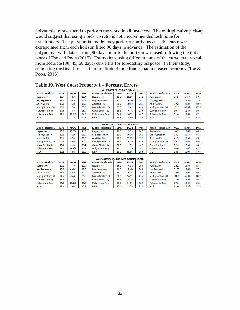
22

polynomial models tend to perform the worst in all instances. The multiplicative pick-up

would suggest that using a pick-up ratio is not a recommended technique for

practitioners. The polynomial model may perform poorly because the curve was

extrapolated from each horizon fitted 90 days in advance. The estimation of the

polynomial with data starting 90 days prior to the horizon was used following the initial

work of Tse and Poon (2015). Estimations using different parts of the curve may reveal

more accurate (30, 45, 60 days) curve fits for forecasting purposes. In their study,

estimating the final forecast in more limited time frames had increased accuracy (Tse &

Poon, 2015).

Table 10. West Coast Property 1 – Forecast Errors

23

Table 11. West Coast Property 2 – Forecast Errors

Table 12. North West Property 1 – Forecast Errors

24

Table 13. Mid-West Property 1 – Forecast Errors

Table 14. MLP – Wilcoxon Hold Out Performance

Table 15. Log Regression – Wilcoxon Hold Out Performance

25

Table 16. Curve Similarity – Wilcoxon Hold Out Performance

Table 17. MLP – Wilcoxon Booking Window Performance

Table 18. Log Regression – Wilcoxon Booking Window Performance

Table 19. Log Regression – Wilcoxon Booking Window Performance

26

Research Question 3

Methodology

The forecast models and results from research question two were leveraged to

answer research question three; whether techniques that leverage the accumulation of

reservations are more robust over time. The techniques that exhibit the Markov Property

and don’t utilize the booking curve are Models 1-4. Specifically, models 1-4 estimate a

pick up from a specific point in time based on historical pick up trends. These techniques

ignore how the reservations accumulated prior to the forecasting date. Models 5, 6, and

the proposed MLP utilize information in how the reservations accumulate at previous

time intervals and leverages that information to generate a forecast.

To statistically identify which models were better suited to combat dynamic

booking windows, the pairwise t-test was implemented to compare the error measures in

the hold out sample to the error measures in the shifted booking window identified in

research question two. The results of each t-test were aggregated across all properties,

error metrics and horizons to identify the general trends. Differences between the two

error metrics were measured at the 0.05 level of significance. Techniques that prove to

be more robust will not have a significant change in error metric between the two time

periods.

Formally

Where is the mean difference between the average error in the hold out sample and the

average error in the sample with the shifted booking window.

Data

The data used to compare the error metrics are the same samples and error metrics

identified in research question two.

Results

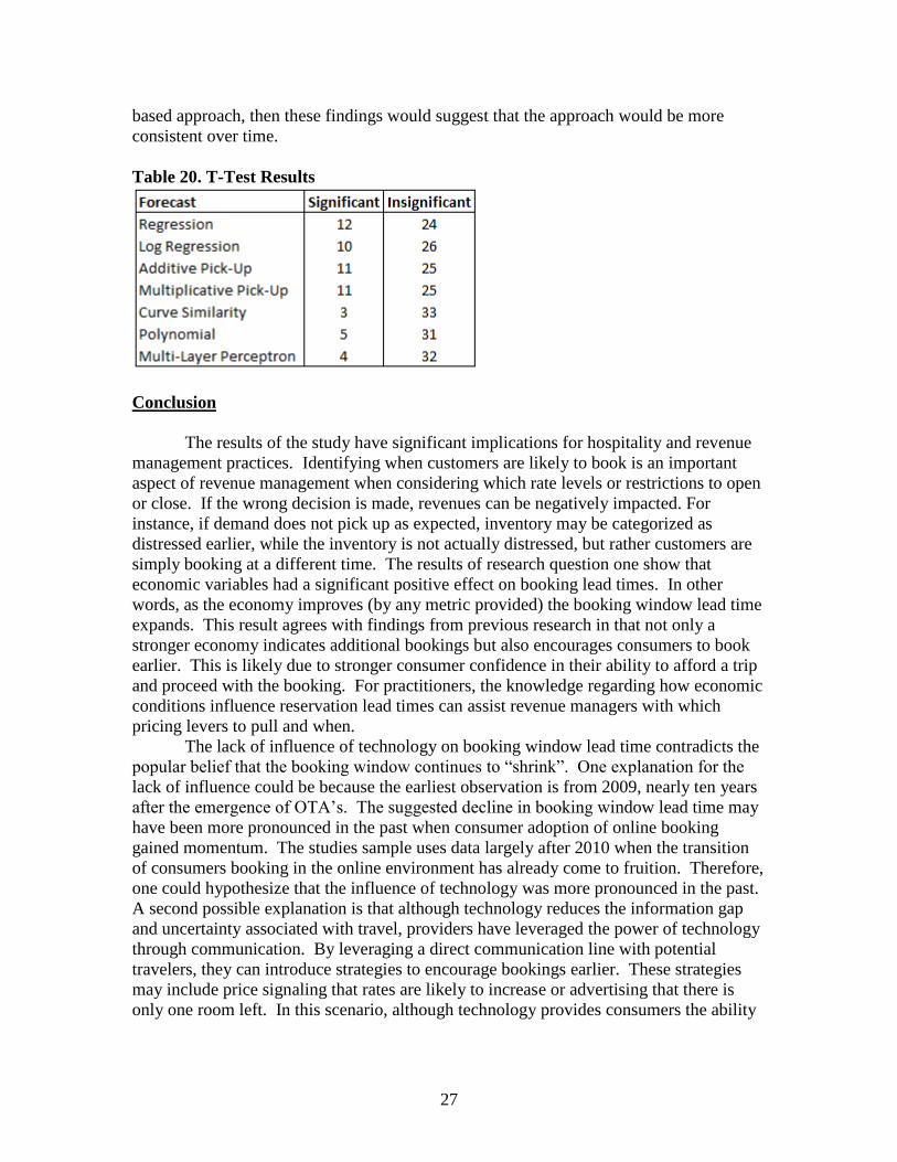
The results of the aggregated t-tests are provided in Table 20. The forecasting

models with the most consistent error metrics between samples were the Curve

Similarity, Polynomial and MLP models. These models had the least number of

significant differences (p<0.05) between error metrics. In addition, these methods all

leverage the information provided in the booking curve and consider how reservations

accumulate. The results of the tests may imply that when forecasting in locations with

fluctuating booking windows, the curve based approaches provide more consistent

estimates than the non-curve based pick-up methods. This may suggest that the curve

based techniques are more robust over time and may be less susceptible to economic

shocks or large booking window shifts. This is likely due to the macro and micro factors

influencing when purchases are occurring and inherently included in how reservations

have accumulated up until the forecast date. If a location can estimate a suitable curve

27

based approach, then these findings would suggest that the approach would be more

consistent over time.

Table 20. T-Test Results

Conclusion

The results of the study have significant implications for hospitality and revenue

management practices. Identifying when customers are likely to book is an important

aspect of revenue management when considering which rate levels or restrictions to open

or close. If the wrong decision is made, revenues can be negatively impacted. For

instance, if demand does not pick up as expected, inventory may be categorized as

distressed earlier, while the inventory is not actually distressed, but rather customers are

simply booking at a different time. The results of research question one show that

economic variables had a significant positive effect on booking lead times. In other

words, as the economy improves (by any metric provided) the booking window lead time

expands. This result agrees with findings from previous research in that not only a

stronger economy indicates additional bookings but also encourages consumers to book

earlier. This is likely due to stronger consumer confidence in their ability to afford a trip

and proceed with the booking. For practitioners, the knowledge regarding how economic

conditions influence reservation lead times can assist revenue managers with which

pricing levers to pull and when.

The lack of influence of technology on booking window lead time contradicts the

popular belief that the booking window continues to “shrink”. One explanation for the

lack of influence could be because the earliest observation is from 2009, nearly ten years

after the emergence of OTA’s. The suggested decline in booking window lead time may

have been more pronounced in the past when consumer adoption of online booking

gained momentum. The studies sample uses data largely after 2010 when the transition

of consumers booking in the online environment has already come to fruition. Therefore,

one could hypothesize that the influence of technology was more pronounced in the past.

A second possible explanation is that although technology reduces the information gap

and uncertainty associated with travel, providers have leveraged the power of technology

through communication. By leveraging a direct communication line with potential

travelers, they can introduce strategies to encourage bookings earlier. These strategies

may include price signaling that rates are likely to increase or advertising that there is

only one room left. In this scenario, although technology provides consumers the ability

28

to delay a purchase, the strategies used by companies to encourage a purchase counteract

the potential delay, causing no change in reservation lead time from technology.

Forecasting in dynamic booking windows presents significant challenges to

practitioners because these forecasts feed revenue management optimization algorithms

and dictate rate decisions. The importance of an accurate forecast cannot be understated

as error reduction can contribute significant increases in revenue (Koupriouchina et al.

2014). The results of research question two would suggest that using a multi-layer

perceptron model may provide revenue management practitioners with another suitable

forecasting approach. Neural networks can model any type of data (categorical or

interval) while also relaxing several assumptions required for many forecasting

approaches. The simple architecture in this study leveraging current data as the input

vector could be enhanced by adding additional data points such as, the day of week,

month, or historical totals on similar days for increased accuracy.

With regards to the importance of including how reservations accumulate in forecasting

model estimations, the results of research question three suggests that curve based

approaches provide more robust models. While it is recommended that practitioners

evaluate a range of methods for forecasting in dynamic booking windows, the results

show that these models are less impacted by changes in the booking window lead time

and should provide practitioners with increased accuracy over a longer duration. These

results are likely attributed to the fact that how the reservations accumulate prior to the

forecast help to depict the current consumption climate as well as the macro and micro

factors that may be influencing the pace of booking. Leveraging information from

previous curves that follow the same pattern, allows for model estimation on data from

bookings that may have occurred under similar conditions in the past. The results of this

study suggest that industry professionals who use curve based forecasting approaches

will likely experience more accurate forecasts over time. These techniques will also

require less re-estimation in comparison to the traditional pick up methods, thus

providing a more autonomous forecasting system.

Limitations

There are several limitations of the study that should be considered when

interpreting results. In the regression analysis, the booking window shifts are analyzed

across 15 properties which should not be considered an accurate representation of all

properties in the United States. The results and patterns for booking window behavior

may be different at properties not located in and around national parks. As the focus of

the study was to try and observe leisure traveler booking patterns, the results may be

different for properties located in urban and suburban areas that have different types of

guests such as business travelers with different booking behaviors.

The forecasting analysis also has several limitations as the models were estimated

on only four properties located around national parks. The accuracy of the models may

provide different results for properties located in different geographic locations with

different targeted markets. The goal of focusing on leisure travelers and their shifts in

booking behavior was met with the national parks data used in this study, however,

further investigation is necessary to formally suggest the most robust forecasting methods

for hotel reservations.

29

Future Research

Several areas of future research are present from the results of this study. The

first is the importance of the economy in booking window fluctuations and travel

purchase patterns. Leveraging economic indicators into the forecasting models may

prove more accurate for forecasting in dynamic booking windows and help account for

their shifts. A second area of future research is the lack of shift in booking behavior due

to technology. The results allow one to hypothesize that the shift in booking behavior

due to technology may have been more pronounced in the past. Obtaining a data set with

reservation accumulations prior to internet reservations, as well as when internet

reservations took off may further confirm that the large booking window shift occurred

years back and is not significant today. A third area for future research is a further

investigation into the benefits of neural networks for forecasting in hospitality revenue

management. Several other techniques such as the Kohonen Self Organizing Map

(SOM) may prove superior for forecasting with current data and identifying booking

window patterns. In addition, hospitality research has yet to leverage neural networks to

combine the three data techniques (historical, current and exogenous information) for

revenue management purposes. Specifically, studies tend to generate weighted averages

of different forecasting techniques to construct a final forecast. Neural networks may be

able find the optimal combinations of the data without having to estimate and test

combinations of all the different data techniques. In this instance, neural networks may

provide a solution for combining forecasting techniques together.

30

References

1. Alegre, J., & Pou, L. (2004). Micro-economic determinants of the probability of tourism consumption. Tourism Economics, 10(2), 125-144.

2. Barthel, J and Perret, S. (2015) OTAs – A Hotel’s Friend or Foe? How Reliant are

Hotels on OTAs?, Hospitality Net, http://www.hotelleriequebec.com/wp-content/uploads/2015/07/HVS-OTAs-–-A-Hotels-Friend-Or-Foe.pdf

3. Bloomberg (2016) Travelocity

http://www.bloomberg.com/research/stocks/private/snapshot.asp?privcapId=411110

4. Cho, V. (2001). Tourism forecasting and its relationship with leading economic

indicators. Journal of Hospitality & Tourism Research, 25(4), 399-420.

5. Choi, J. G. (2003). Developing an economic indicator system (a forecasting technique) for the hotel industry. International Journal of Hospitality Management, 22(2), 147-159.

6. Choi, S., & Kimes, S. E. (2002). Electronic distribution channels’ effect on hotel

revenue management.

7. Carroll, B., & Siguaw, J. (2003). Evolution in electronic distribution: Effects on hotels and intermediaries.

8. Chen, C., & Kachani, S. (2007). Forecasting and optimisation for hotel revenue

management. Journal of Revenue & Pricing Management, 6(3), 163-174.

9. Crouch, G. I. (1994). The study of international tourism demand: a review of findings. Journal of Travel research, 33(1), 12-23.

10. Crouch, G. I. (1994). The study of international tourism demand: a survey of practice. Journal of Travel research, 32(4), 41-55.

11. Dacko, S. G. (2004). Marketing strategies for last-minute travel and tourism:

Profitability and revenue management implications. Journal of Travel & Tourism Marketing, 16(4), 7-20.

12. Duran, Juan Understanding Online Distribution Channels, Jun 15, 2015

http://www.hvs.com/article/7380/understanding-online-distribution-channels/

http://www.hotelleriequebec.com/wp-content/uploads/2015/07/HVS-OTAs-–-A-Hotels-Friend-Or-Foe.pdf

http://www.hotelleriequebec.com/wp-content/uploads/2015/07/HVS-OTAs-–-A-Hotels-Friend-Or-Foe.pdf



http://www.hvs.com/article/7380/understanding-online-distribution-channels/

31

13. Empson, Rip 2012 November 22, 2012 KAYAK https://techcrunch.com/2012/11/22/follow-the-money-why-priceline-bought-kayak/

14. Flores, B. E. (1989). The utilization of the Wilcoxon test to compare forecasting methods: A note. International Journal of Forecasting, 5(4), 529-535.

15. Garson, David (2014) Neural Network Models. Statistical Associates, 1-144.

16. Gasdia, Marcello (2015) Mobile travel shopping hits tipping point – But PC still

dominates booking Phocuswright http://www.phocuswright.com/Travel-Research/Research-Updates/2015/Mobile-Travel-Shopping-Hits-Tipping-Point-But-PC-Still-Dominates-Booking

17. Granados, N., Gupta, A., & Kauffman, R. J. (2012). Online and offline demand and

price elasticities: Evidence from the air travel industry. Information Systems Research, 23(1), 164-181.

18. Granger, C. W. (1993). Strategies for Modelling Nonlinear Time‐Series

Relationships. Economic Record, 69(3), 233-238.

19. Hyndman, R. J., & Athanasopoulos, G. (2014). Forecasting: principles and practice. OTexts.

20. Ismail, J. A., Dalbor, M. C., & Mills, J. E. (2002). Using RevPAR to analyze lodging-

segment variability. Cornell Hospitality Quarterly, 43(6), 73.

21. Jang, S. (2005). The past, present, and future research of online information search. Journal of Travel & Tourism Marketing, 17(2-3), 41-47.

22. Kim, S. Y. (2011). Prediction of hotel bankruptcy using support vector machine,

artificial neural network, logistic regression, and multivariate discriminant analysis. The Service Industries Journal, 31(3), 441-468.

23. Koupriouchina, L., van der Rest, J. P., & Schwartz, Z. (2014). On revenue

management and the use of occupancy forecasting error measures. International Journal of Hospitality Management, 41, 104-114.

24. Law, R. (1998). Room occupancy rate forecasting: a neural network approach.

International Journal of Contemporary Hospitality Management, 10(6), 234-239.

25. Law, R., & Au, N. (1999). A neural network model to forecast Japanese demand for travel to Hong Kong. Tourism Management, 20(1), 89-97.

https://techcrunch.com/2012/11/22/follow-the-money-why-priceline-bought-kayak/

https://techcrunch.com/2012/11/22/follow-the-money-why-priceline-bought-kayak/

http://www.phocuswright.com/Travel-Research/Research-Updates/2015/Mobile-Travel-Shopping-Hits-Tipping-Point-But-PC-Still-Dominates-Booking



32

26. Lee, A. O. (1990). Airline reservations forecasting: Probabilistic and statistical models of the booking process. Cambridge, Mass.: Flight Transportation Laboratory, Dept. of Aeronautics and Astronautics, Massachusetts Institute of Technology.

27. Lee, T (2013). Top 10 Trends of The Next Generation of Travel: The Millennials

Hotel Online available at: http://www.hotel-online.com/News/PR2013_2nd/Apr13_MillennialTrends.html

28. Lloyd-Jones, A. R. (2005). What happens to occupancy and average rate in a

slowing economy?. HVS International Journal, 1-3.

29. Mahmoud, Ahmed Hospitality Net – Hotel ADR Rise vs. Distribution Channels Cost, What Hoteliers Need to Calculate? 6/12/2015, http://www.travelclick.com/en/news-events/in-the-news/hospitality-net-–-hotel-adr-rise-vs-distribution-channels-cost-what-hoteliers-need-calculate

30. Manley, B. (2016). Business travel: An evolution in progress. Hotel News Now

available at: http://hotelnewsnow.com/Articles/48528/Business-travel-An-evolution-in-progress

31. Mayock, P. (2011), “Sales teams feel pinch of short booking windows”, HotelNewsNow.com, available at:http://www.hotelnewsnow.com/Articles/11237/Sales-teams-feel-pinch-of-short-booking-windows

32. O'Connor, P., & Frew, A. J. (2002). The future of hotel electronic distribution: Expert and industry perspectives. The Cornell hotel and restaurant administration quarterly, 43(3), 33-45.

33. O’Connor, P. (2002). An Analysis of the Online Pricing Strategies of the

International Hotel Chains, Information and Communications Technologies in Tourism 2002.

34. Park, S. S., & Hancer, M. (2012). A comparative study of logit and artificial neural

networks in predicting bankruptcy in the hospitality industry. Tourism Economics, 18(2), 311-338.

35. Pan, B., Chenguang Wu, D., & Song, H. (2012). Forecasting hotel room demand

using search engine data. Journal of Hospitality and Tourism Technology, 3(3), 196-210.

36. Phillips, R. L. (2005). Pricing and revenue optimization. Stanford University Press.

http://www.hotel-online.com/News/PR2013_2nd/Apr13_MillennialTrends.html

http://www.hotel-online.com/News/PR2013_2nd/Apr13_MillennialTrends.html

http://www.travelclick.com/en/news-events/in-the-news/hospitality-net-–-hotel-adr-rise-vs-distribution-channels-cost-what-hoteliers-need-calculate

http://www.travelclick.com/en/news-events/in-the-news/hospitality-net-–-hotel-adr-rise-vs-distribution-channels-cost-what-hoteliers-need-calculate

http://hotelnewsnow.com/Articles/48528/Business-travel-An-evolution-in-progress

http://hotelnewsnow.com/Articles/48528/Business-travel-An-evolution-in-progress

http://www.hotelnewsnow.com/Articles/11237/Sales-teams-feel-pinch-of-short-booking-windows

http://www.hotelnewsnow.com/Articles/11237/Sales-teams-feel-pinch-of-short-booking-windows

33

37. Rajopadhye, M., Ghalia, M. B., Wang, P. P., Baker, T., & Eister, C. V. (2001). Forecasting uncertain hotel room demand. Information sciences, 132(1), 1-11.

38. Relihan, W. J. (1989). The yield-management approach to hotel-room pricing.

Cornell Hotel and Restaurant Administration Quarterly, 30(1), 40-45.

39. Sahay, A. (2007). How to reap higher profits with dynamic pricing. MIT Sloan management review, 48(4), 53-60.

40. Schwartz, Z., & Hiemstra, S. (1997). Improving the accuracy of hotel reservations

forecasting: curves similarity approach. Journal of Travel Research, 36(1), 3-14.

41. Schwartz, Z. (1998). The confusing side of yield management: Myths, errors, and misconceptions. Journal of Hospitality & Tourism Research, 22(4), 413-430.

42. Schwartz, Z. (2000). Changes in hotel guests’ willingness to pay as the date of

stay draws closer. Journal of Hospitality & Tourism Research, 24(2), 180-198.

43. Schwartz, Z. (2006). Advanced booking and revenue management: Room rates and the consumers’ strategic zones. International Journal of Hospitality Management, 25(3), 447-462.

44. Schwartz, Z. (2008). Time, price, and advanced booking of hotel rooms.

International Journal of Hospitality & Tourism Administration, 9(2), 128-146.

45. Schwartz, Z., & Chen, C. C. (2012). Hedonic motivations and the effectiveness of risk perceptions–Oriented revenue management policies. Journal of Hospitality & Tourism Research, 36(2), 232-250.

46. Schwartz, Z., Uysal, M., Webb, T., & Altin, M. (2016). Hotel daily occupancy

forecasting with competitive sets: a recursive algorithm. International Journal of Contemporary Hospitality Management, 28(2), 267-285.

47. Smeral, E. (1988). Tourism demand, economic theory and econometrics: An

integrated approach. Journal of Travel Research, 26(4), 38-43.

48. Smeral, E. (2009). The impact of the financial and economic crisis on European tourism. Journal of Travel Research.

49. Zheng, T., Bloom, B. A., Wang, X., & SChrIEr, T. (2012). How do Less Advanced

Forecasting Methods Perform on Weekly RevPAR in Different Forecasting Horizons Following the Recession?. Tourism Analysis, 17(4), 459-472.

34

50. Thakran, K., & Verma, R. (2013). The emergence of hybrid online distribution channels in travel, tourism and hospitality. Cornell Hospitality Quarterly, 54(3), 240-247.

51. Thomas, Marita (2016) Orbitz Datehttps://globenewswire.com/news-

release/2016/06/06/846240/0/en/To-Celebrate-Orbitz-com-s-15th-Birthday-Travelers-Can-Win-a-Trip-for-15-Friends.html June 6, 2016

52. Travel Click (2012) Travel Click Business and Leisure Travelers book rooms

further in advance http://www.travelclick.com/en/news-events/press-release/business-and-leisure-travelers-book-hotel-rooms-further-advance

53. Toh, R. S., Raven, P., & DeKay, F. (2011). Selling rooms: Hotels vs. third-party

websites. Cornell Hospitality Quarterly, 52(2), 181-189.

54. Tsai, T. H., Lee, C. K., & Wei, C. H. (2009). Neural network based temporal feature models for short-term railway passenger demand forecasting. Expert Systems with Applications, 36(2), 3728-3736.

55. Tse, T. S. M., & Poon, Y. T. (2015). Analyzing the Use of an Advance Booking

Curve in Forecasting Hotel Reservations. Journal of Travel & Tourism Marketing, 32(7), 852-869.

56. Uysal, M., & El Roubi, M. S. (1999). Artificial neural networks versus multiple

regression in tourism demand analysis. Journal of Travel Research, 38(2), 111-118.

57. Vellido, A., Lisboa, P. J., & Vaughan, J. (1999). Neural networks in business: a

survey of applications (1992–1998). Expert systems with applications, 17(1), 51-70.

58. Weatherford, L. R., Gentry, T. W., & Wilamowski, B. (2003). Neural network

forecasting for airlines: A comparative analysis. Journal of Revenue and Pricing Management, 1(4), 319-331.

59. Weatherford, L. R., & Kimes, S. E. (2003). A comparison of forecasting methods

for hotel revenue management. International Journal of Forecasting, 19(3), 401-415.

60. Weatherford, L. R., Kimes, S. E., & Scott, D. A. (2001). Forecasting for hotel

revenue management: Testing aggregation against disaggregation.

http://www.travelclick.com/en/news-events/press-release/business-and-leisure-travelers-book-hotel-rooms-further-advance

http://www.travelclick.com/en/news-events/press-release/business-and-leisure-travelers-book-hotel-rooms-further-advance

35

61. Webb, T. (2016). From travel agents to OTAs: How the evolution of consumer booking behavior has affected revenue management. Journal of Revenue and Pricing Management.

62. Worgull, Samantha Hotel News Now August 29,2013

http://www.hotelnewsnow.com/Articles/20146/Travelers-trip-planning-habits-are-evolving

63. Yang, Y., Pan, B., & Song, H. (2014). Predicting hotel demand using destination

marketing organization’s web traffic data. Journal of Travel Research, 53(4), 433-447.

64. Yesawich, Pepperdine and Brown (2000). National leisure travel monitor.

Orlando, FL: Yesawich, Pepperdine and Brown http://www.hotel-online.com/News/PR2001_1st/Jan01_GHAYesawich.html

65. Youn, H., & Gu, Z. (2010)a. Predict US restaurant firm failures: The artificial

neural network model versus logistic regression model. Tourism and Hospitality Research, 10(3), 171-187.

66. Youn, H., & Gu, Z. (2010)b. Predicting Korean lodging firm failures: An artificial

neural network model along with a logistic regression model. International Journal of Hospitality Management, 29(1), 120-127.

67. Zhang, G., Patuwo, B. E., & Hu, M. Y. (1998). Forecasting with artificial neural

networks: The state of the art. International journal of forecasting, 14(1), 35-62.



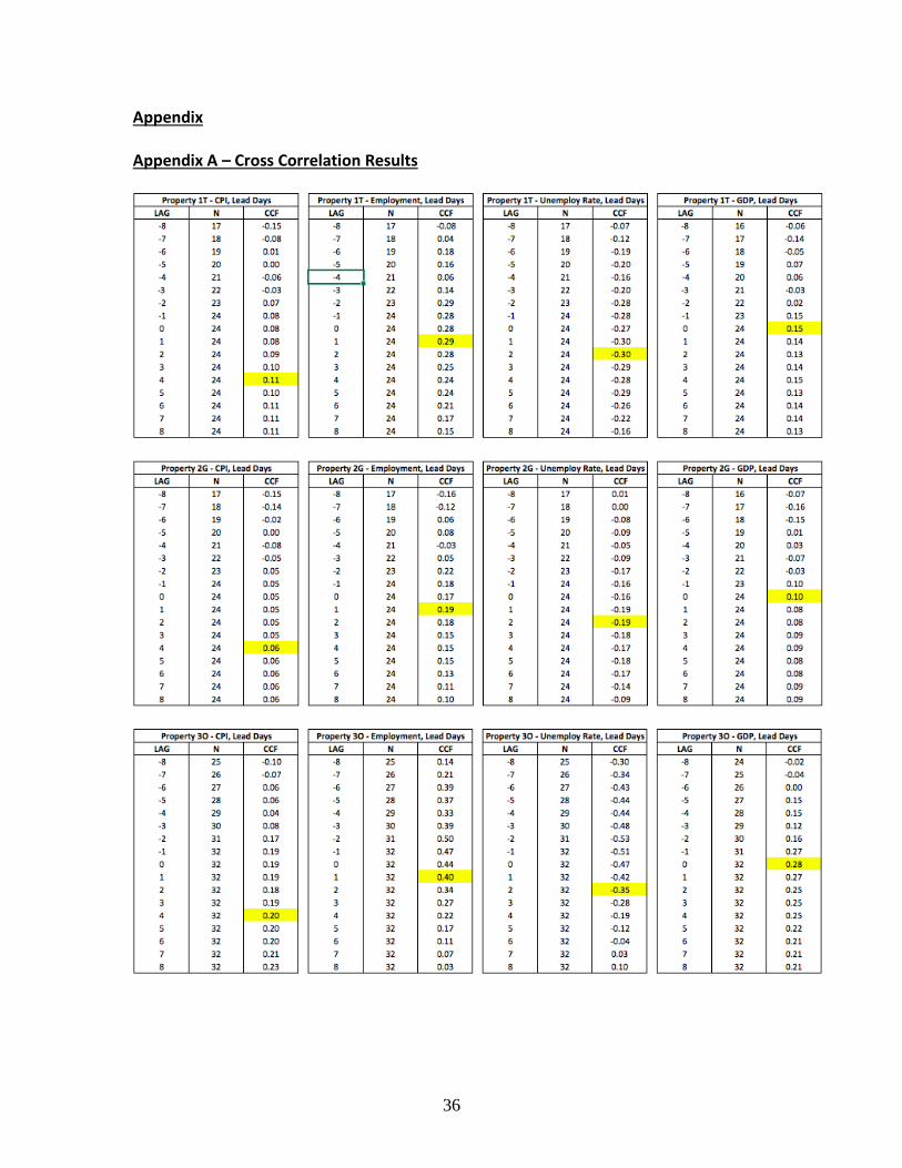
http://www.hotel-online.com/News/PR2001_1st/Jan01_GHAYesawich.html

http://www.hotel-online.com/News/PR2001_1st/Jan01_GHAYesawich.html

36

Appendix Appendix A – Cross Correlation Results

37

Appendix B - Absolute Error Wilcoxon Test Results The results of the Wilcoxon Signed Rank Tests are provided in the corresponding tables. The estimate of the metric infers which method may be superior based on how the test was performed. A negative sign implies the model on the left-hand side of the table is more accurate while a positive sign indicates the model on the top is more accurate. The p-values are recorded in the sequential table which depicts if the model is superior to the others.

The Booking Window Evolution and its Impact on Hotel ... · reservation was made to a travel agent,...

Documents

Transcript of The Booking Window Evolution and its Impact on Hotel ... · reservation was made to a travel agent,...