Statistical-Empirical Modelling of Aerofoil Noise ... · Frank Kameier 3 Duesseldorf University of...

American Institute of Aeronautics and Astronautics

1

Statistical-Empirical Modelling of Aerofoil Noise Subjected to Leading Edge Serrations and Aerodynamic Identification

of Noise Reduction Mechanisms

Till Biedermann1 Duesseldorf University of Applied Sciences, Duesseldorf, D-40474, Germany

Tze Pei Chong2 Brunel University London, London, UB83PH, UK

and

Frank Kameier3 Duesseldorf University of Applied Sciences, Duesseldorf, D-40474, Germany

With the objective of reducing the broadband noise, emitted from the interaction of highly turbulent flow and aerofoil leading edge, sinusoidal leading edge serrations were analysed as an effective passive treatment. An extensive aeroacoustic study was performed in order to determine the main influences and interdependencies of factors, such as the Reynolds number (Re), turbulence intensity (Tu), serration amplitude (A/C) and wavelength (λ/C) as well as the angle of attack (AoA) on the noise reduction capability. A statistical-empirical model was developed to predict the overall sound pressure level and noise reduction of a NACA65(12)-10 aerofoil with and without leading edge serrations in the analysed range of chord-based Reynolds numbers of 2.5·105 ≤ Re ≤ 6·105 and a geometrical angle of attack -10 deg ≤ α ≤ +10 deg. The observed main influencing factors match current research results to a high degree, and were quantified in a systematic order for the first time. Moreover, significant interdependencies of the turbulence intensity and the serration wavelength (Tu·λ/C), as well as the serration wavelength and the angle of attack (λ/C·AoA) were observed, validated and quantified. In order to study the noise reduction mechanisms, Particle Image Velocimetry (PIV) measurements were conducted upstream of the aerofoil leading edge and along the interstices of the leading edge serrations. Velocity, turbulence intensity and vorticity in the plane perpendicular to the main flow direction (y/z plane) were analysed and linked to the acoustic findings. It was observed that a noise reduction is accompanied by a reduction of the turbulence intensity within the serration interstices. The reduction in turbulence intensity is more pronounced with large serration amplitudes. However, the impact of the serration wavelength was found to be no function of the turbulence. It is more likely to be affected acoustically by spanwise de-correlation effects as a response to the incoming gusts.

Nomenclature A = amplitude of leading edge serrations [mm] λ = wavelength of leading edge serrations [mm] U0 = free stream velocity [ms-1] Tu = turbulence intensity [%] Re = cord-based Reynolds number [--] AoA = angle of attack, defined as y/H [..] 1 Research Assistant, Institute of Sound and Vibration Engineering ISAVE, [email protected], Non-AIAA Member 2 Senior Lecturer, Department of Mechanical, Aerospace and Civil Engineering, AIAA Member 3 Professor, Institute of Sound and Vibration Engineering ISAVE, Non-AIAA Member


2

C = aerofoil chord length [mm] S = aerofoil span [mm] H = nozzle height [mm] HMax = maximum aerofoil thickness [mm] AoA = angle of attack [°] x = local streamwise (longitudinal) coordinate [mm] y = local anti-streamwise (transversal) coordinate [mm] z = local vertical coordinate [mm] OASPL = overall sound pressure level [dB] ΔOASPL = overall sound pressure level reduction [dB] pSerr/pBL = non-dimensional, fractional sound pressure [--] f = frequency [Hz] ΔSPL = sound pressure level reduction [dB] ω = angular frequency [s-1] Θ = polar angle [deg] Ma = Mach number [--] LE = aerofoil leading edge

I. Introduction ECENT research has firmly established sinusoidal leading edge (LE) serrations as an effective passive treatment to reduce the emitted broadband noise of an aerofoil exposed to a highly turbulent flow. A reduction in the overall

sound pressure level of up to ΔOASPL = 7dB and local sound pressure level reductions above ΔSPL = 10dB in the relevant frequency region could be reached.1–4 Several parameters have been found to influence the effectiveness of noise reduction by leading edge (LE) serrations, which include the Reynolds number (Re), turbulence intensity (Tu), serration amplitude (A/C), serration wavelength (λ/C) and angle of attack (AoA). However, up to now, these parameters have been regarded independently, and only little effort was made to analyse them as an interrelated system of factors with respect to the noise reduction. This serves as motivation for the current work, where a comprehensive statistical-empirical model has been developed with the aim to describe the noise emittance and reduction of serrated LE as an interrelated system of several influencing parameters. As it is shown in Section IV-C, the developed model even shows good fit and accurate predictions of the emitted noise when applied to an external experimental environment.

Although different hypotheses on the noise reduction mechanism were proposed before, they have hitherto not been comprehensively verified. In general, three mechanisms have been identified that could be responsible for the reduction in broadband noise. First is the reduced spanwise correlation coefficients as a result of incoherent response times of the incoming turbulence; second, a reduction of the acoustic sources as manifested in the reduction in RMS pressure fluctuation at the serration peak; and, third, a reduction of the streamwise turbulence intensity due to the converging flow within the serrations.5; 6

Up to now, research on the effect of LE serrations focussed either on the noise reduction capability, or on the aerodynamic advantages of the performance of the aerofoil itself. The effect of sinusoidal LE on the lift and drag forces has been analysed experimentally, numerically and through the use of flow pattern visualisation.7; 8 A numerical study to optimise the serration design in order to improve the aerodynamic forces on the aerofoil was presented.9 The commonality of the recent research is the focus on describing the flow, starting at the serration surface. In contrast, a numerical study has been recently published, in which pressure and velocity distributions are analysed at distinct streamwise locations, starting upstream of the LE.5 However, no information is available so far to describe the effect of different serration parameters on the flow in front of and within the interstices of the serrated LEs.

Of particular importance is the correlation between the aerodynamic flow behaviours and aeroacoustic noise reduction mechanisms. In general, the incoming turbulence amplifies the surface pressure fluctuations close to the aerofoil LE, which then radiate into broadband noise10; 11. The serrated LEs, on the other hand, cause a significant decrease in the surface pressure fluctuations and subsequently reduce the broadband noise level. The converging nature of the serration could generate a nozzle effect to accelerate the flow within and reduce the level of turbulence intensity before the fluid-structure interaction near the stagnation points. Therefore, it is plausible to analyse the noise reduction mechanism in terms of the aerodynamics behaviours in front of and within the interstices of the serrations for different serration parameters. This provides a motivation in the current study to perform Particle Image Velocimetry (PIV) experiments to gain a deeper understanding of the underlying principles, and then to use the results to enhance the acoustic noise reduction capability of future applications.

R


3

II. Experimental Setup In the current study, a cambered NACA65(12)-10 aerofoil was utilised, due to its similarity to real-life application

such as the stator vanes or axial fan blades. As shown in Fig. 1, the aerofoil has a chord length of C = 150 mm and a span width of S = 300 mm. Between the leading edge (x/C = 0) and x/C = 0.3, there is a section that can be removed and replaced by different serration profiles. Note that x is the streamwise direction. Further downstream, 0.3 < x/C < 1.0, is the unmodified aerofoil main body. Once attached, the serrations form a continuous profile giving the appearance that they are cut into the main body of the aerofoil. The serration geometry is defined by two parameters: amplitude (chordwise peak-to-trough value) and wavelength (spanwise peak-to-peak-value). Both parameters are normalised by the aerofoil chord length C = 150 mm. The angle of attack is defined as a non-dimensional ratio of vertical LE tip displacement (y) and the height of the nozzle outlet (H), giving AoA ≈ y/H at small angle of attack. The shape of the LE serrations is designed according to a sinusoidal curve, and the NACA65(12)-10 profile was extruded along the line of this curve. An important feature of the current design is the semi-cyclic shape of the serration tips.

Figure 1. NACA65(12)-10 aerofoil main body and re-attachable leading edge with measures of importance for the acoustical treatment in the open jet stream.15; 16

Experiments were conducted in the aeroacoustics facility at Brunel University London where an open jet wind tunnel is situated in a 4 m x 5 m x 3.4 m semi-anechoic chamber.17 The nozzle exit is rectangular with dimensions of 0.10 m (height) x 0.30 m (width). The wind tunnel can achieve a minimum turbulence intensity of 0.1 – 0.2 %. The maximum jet velocity is about 80 ms-1. In order to achieve high turbulence intensities (Tu), grids of various spacing were used. Adopting the criteria set by Laws and Livesey18, all grids are biplane square meshes with a constant ratio of bar diameter and mesh size (M/d = 5). Using the turbulence prediction model by Aufderheide et al.19 which is based on the work of Laws and Livesey18, five different grids for the generation of Tu in the range of 2.1 % ≤ Tu ≤ 5.5 % were defined and verified experimentally. The integral length scale of the turbulent eddies was found to be a function of Tu, but it was not included as an integral parameter for the noise modelling analysis.

The turbulence intensity near the aerofoil’s LE is assumed isotropic. In this context, the analysis of the measured power density spectra showed a good agreement with both turbulence models (Fig. 2) of von Kármán and Liepmann in Eq. (1), after having applied the correction function of Rozenberg20 in Eq. (2) in order to take the dilution in the high-frequency region close to the Kolmogorov scale into account. �� is the velocity fluctuation, �� is the integral length scale, �� the streamwise wave number and � a constant that controls the gradient of the roll off at high frequencies. The lower limit of the investigated chord-based Reynolds number was determined by the required isotropic condition of the Tu, whereas the upper limit was dictated by the fan capacity in the experimental setup (2.5·105 ≤ Re ≤ 6·105).

�� ′2��0 ∙ 1

1��2��2 (1)

��. � �! "#$9 4' ( ∙ )�� * +�, (2)

y

z x


4

Figure 2. Normalised turbulence energy spectrum according to Liepmann at 30ms-1 ≤ U0 ≤ 60ms-1, Tu =

3.9%, measured at the imaginary location of the aerofoil leading edge. Applied correction for high-frequency dilution according to Rozenberg.20

The conducted experimental study can be subdivided into an aeroacoustic and an aerodynamic study. In the aeroacoustic study (Section IV), a statistical-empirical model describes the acoustic response, as a function of five influencing parameters. In the aerodynamic study (Section V), the flow patterns in front of the serrations and within the interstices of the serrations are analysed by the Particle Image Velocimetry (PIV) technique. Although these aeroacoustic and aerodynamic experiments were carried out independently, the results are supplementary to each other where a causal relationship between the flow patterns and the aeroacoustic results for a selected LE configuration is established.

A. Aeroacoustic Measurement Technique Because of the chosen parameters of the Design of Experiments (DoE), which will be discussed in Section III, a

total of ten leading edge sections were investigated. These include one configuration with a straight LE to serve as the baseline case. Free field measurements of the AGI-Noise (Aerofoil-Gust-Interaction) were conducted in the aeroacoustic facility at Brunel University London.21 The aerofoil was held by side plates and attached flushed to the nozzle lips. Noise measurements at the aeroacoustic wind tunnel were made by a PCB ½-inch prepolarised ICP® condenser microphone at polar angles of Θ = 90 degree at a distance of 0.95 m from the LE of the aerofoil at mid-span. The acoustic data was recorded at a sampling rate of SR = 40 kHz, with a blocksize of BZ = 1024. The feasible frequency range for the data analyses was set to 300 Hz ≤ fAnalyse ≤ 10 kHz, where the lower limit is due to the cut-off frequency of the anechoic chamber. The upper limit was chosen in order to avoid the possible influences by aerofoil self-noise, which is not related to aerofoil-gust-interaction. The range of jet speeds under investigation is between 25 ms-1 and 60 ms-1, corresponding to Reynolds’ numbers based on the aerofoil chord length of 2.5∙105 ≤ Re ≤ 6∙105 respectively.

As shown in Table 1, the levels for each of the five investigated parameters were defined. Upper and lower levels are set as a consequence of the fan capacity, the maximum grid-generated turbulence and the restrictions of the experimental setup. Intermediate levels are set by the choice of the measurement plan and the statistical features of the future model, as described in Section III.

Table 1. Non-dimensional DoE (Design of Experiments) levels of the different factors of interest. Serration amplitude and wavelength normalised by aerofoil chord (C = 150mm); angle of attack normalised by nozzle

height (H = 100mm). Unit -αDoE -1DoE 0DoE +1DoE +αDoE

xNondim -- -2.3784 -1.0 0.0 +1.0 +2.3784

Re -- 250,000 351,422 425,000 498,578 600,000 Tu(u) % 2.08 3.07 3.79 4.51 5.50

ASerr /C -- 0.080 0.144 0.190 0.236 0.300 λSerr /C -- 0.050 0.122 0.175 0.228 0.300

y/H -- -0.128 -0.054 0.000 0.054 0.128


5

In order to ensure valid measurements, where the background noise of the wind tunnel facility is well below the AGI-Noise, preliminary measurements were performed at extreme flow conditions prior to the main acoustic study. At minimum and maximum fan speed, the acoustic signature of the background noise, the baseline aerofoil and the aerofoil with the expected capacity in maximum noise reduction (A45λ7.5) were measured. The acoustic results are shown in Fig. 3. The angle of attack was chosen to be constant at zero degrees, and the Tu is, according to Eq. 3, set to the maximum at 5.5 %. The plot of the narrow band spectrum in Fig. 3 illustrates that the ambient noise without the presence of an aerofoil in front of the nozzle outlet shows a significant lower sound pressure level compared to both the aerofoil cases. The sound pressure level in the case of the aerofoil with a straight LE (baseline case) is always below the emitted sound of an aerofoil with a serrated LE, especially in the intermediate frequency region of interest between 300 Hz and 4 kHz, where the main contribution of the noise reduction is expected to come from the serrations.

Figure 3. Comparison of emitted narrow band spectrum of aerofoil at Re = 250,000 and Re = 600,000 with

baseline (straight) and serrated leading edge (dashed). Additional plot of the sound spectrum without attached aerofoil (dotted). Results at highest investigated turbulence intensity and zero angles of attack. The

OASPL is indicated in the box.

B. Particle Image Velocimetry Setup Particle Image Velocimetry (PIV) was used to trace the movement of seeded particles, illuminated by a laser light

sheet. The PIV allows a two-dimensional velocity field measurement that could compensate the lack of spatial resolution by point measurements (e.g. hot wire probe). Moreover, the presence of a hot wire probe could have some negative impacts on the flow in front of and within the interstices of the serrations. The PIV experiments took place in the anechoic chamber of the aeroacoustic wind tunnel at Brunel University London.21 The experimental arrangement is illustrated in Fig. 4a.

When the aerofoil is attached to the exit nozzle with side plates, a laser light sheet is projected upwards at Θ = 90-degrees polar angle from a platform underneath the aerofoil. If [x, y, z] denote the longitudinal, transversal and vertical directions, respectively, the laser light sheet will be in the [y, z] plane. A Litron® Nd:YAG-Laser with two cavities was used as a source for the laser beam, which radiated at wavelengths of 1064 nm (infrared) and at a pulsing frequency of 15 Hz.

Polyethylene glycol (PEG) was dispersed to droplets of a diameter of 1.5 μm ≤ d ≤ 2.5 μm. The seeded particles were injected on the inlet of the centrifugal fan outside of the anechoic chamber. After passing through the diffuser, the silencers and a series of flow conditioning devices of the acoustic wind tunnel, the particles reach the nozzle, where the flow is accelerated before it can finally discharge into the atmosphere and impinge on the aerofoil. The injected particles show a homogeneous distribution when reaching the measurement plane (Fig. 4b).

A CCD (charge-coupled device) camera was positioned downstream at a distance of 1.3 metres of the aerofoil to trace the illuminated particles. Although the on-axis positioning of the camera is preferable, it cannot be realised due to the setup restrictions, and the necessity to observe the leading edge of the aerofoil that would have been blocked by the aerofoil main body at a horizontal alignment. A vertical angle of 27.8 degrees was found to be sufficient to ensure monitoring beyond the aerofoil main body. According to the pulsing frequency, the camera captured 15 double frames per second, where the time delay between each pair of frames was 3.5 μs in order to track the movement of particles in the 2 mm thick light sheet. Therefore, the real resolution in time is much higher than 15 Hz, although there is a lack of data in-between, analogue to old frequency analysers, which were not capable of real-time analysis.

103

1040

10

20

30

40

50

60

70

80

f, Hz

SP

L, d

B

BL, Re 2.5e5, 71.7 dBSerr, Re 2.5e5, 63.2 dBw/o, Re 2.5e5, 54.1 dBBL, Re 6.0e5, 93.6 dBSerr, Re 6.0e5, 88.1 dBw/o, Re 6.0e5, 74.4 dB

Tu = 5.5 %

-�� .�� /* (3)


6

Figure 4. a) Sketch of experimental PIV setup. b) Laser plane (y/z-plane) with illuminated PEG particles at the tip of serrated leading edge.

In order to compensate the possible image distortion due to the off-axis camera, an image-model fit was applied to the captured frames for the purpose of dewarping and perspectively transforming the skewed images to those if viewed from a normal angle. Based on a mathematical model, the model fit describes how points in the object plane (mm-scale) are transformed into the image plane (pixel-scale). The captured and dewarped double frames enable analysing the signal via a cross or an adaptive correlation. Equation 4 shows the underlying normalised cross-correlation function for the same interrogation area of two frames. It describes two series as a function of the lag. The resulting values vary between [-1, 1], where 1 represents a perfect correlation, and 0 represents no correlation at all

0120∑ #45�6,8�245(#49�6,8�249(:;5:;96,8 (4)

N is the number of pixels, F1, F2 are the interrogation areas (IA) of both images, <0, <� the mean values of the IA and =40, =4� the standard deviation of the IA.23 The velocity field of planes that stretched along the aerofoil span and height (y/z-plane) was obtained by the use

of an adaptive correlation, which is based on the cross-correlation, but uses a varying interrogation area. Starting at a large initial IA (128 x 128 pixels) with a high signal-to-noise ratio (S/N ratio), it performs a cross-correlation before reducing the IA and using the calculation results as an input parameter for the next step until the final IA size (16 x 16 pixels) is reached. After analysing the acquired data, each performed correlation was checked regarding the amount of substituted vectors (Fig. 5a). A significant amount of such vectors required an increase of the final IA. Moreover, a sporadic comparison between the results of an adaptive- and a cross-correlation allows an estimation of the validity and the quality of the obtained results.

a)

b)

z/w x/u

y/v


7

Figure 5. a) Data capturing and post-processing. b) NACA 65 (12)-10 with slices in y/z-plane.

A set of five different serrations as well as the baseline LE were analysed at five distinct streamwise locations each (Fig. 5b), and at zero angles of attack (AoA = 0 deg). The chosen serration amplitude (A/C) and wavelength (λ/C) cover the extremes of the previously conducted aeroacoustic study. Due to restriction in the experimental setting, only [v, w] velocity components were recorded (Fig. 4a). The free stream velocity was limited to a low level of U0 = 20 ms-1 in order to prevent slip effects of the seeded particles. The upper frequency of the turbulent velocity fluctuations should increase with the freestream velocity, and the particles of the used diameter 1.5 μm ≤ d ≤ 2.5 μm are not able to follow the fluctuations at frequencies higher than 10 kHz. Additionally, too high velocities will lead to difficulties in achieving the optimum particle density and signal quality for valid PIV data. The streamwise turbulence intensity, the main cause for the broadband LE noise, was set to the maximum of Tu = 5.5 %. As Table 2 indicates, the execution of experiments at all distinct locations was prohibited by limitations, due to the blocking of the visible area by the aerofoil main body.

Table 2. Measurement matrix for each streamwise location, varying from -5 mm (in front of the serration) to +15 mm (within serration interstices). X indicates conducted, -- not conducted experiment.

No. Label A/C λ/C Tu y/H Re Streamwise loc. [mm] [--] [--] [--] [--] % [--] [--] -5

-1

+2

+5

+10

+15

1 A12λ26 0.08 0.175 5.1 0 200,000 x x x x -- -- 2 A45λ26 0.30 0.175 5.1 0 200,000 x x x x x x 3 A29λ7.5 0.19 0.050 5.1 0 200,000 x x x -- -- -- 4 A29λ45 0.19 0.300 5.1 0 200,000 x x x x x x 5 A29λ26 0.19 0.175 5.1 0 200,000 x x x x x x 6 BL -- -- 5.1 0 200,000 x x -- -- -- --

The post analysis of the experimental data focuses on the evaluation of three parameters: velocity, turbulence

intensity and streamwise vorticity. Note that [w] and [v] refer to the vertical and spanwise components of the velocity, respectively. In this study, the [w] velocity component was found to be the dominant parameter at regions close to the serrations where only a minor effect of the [v] component was observed. For brevity, the analysis of the PIV results thus only focuses on the [w] component of the velocity. Equation 5 shows the definition of turbulence intensity based on the vertical velocity Tu(w). Note that the local mean value of the vertical velocity >/ was adopted as the normalisation parameter because the streamwise velocity component [u] was not measured in the PIV experiment. This definition is different to the streamwise turbulence intensity Tu(u) as defined in Eq. 3 in Section II-A, which was measured by a hot wire probe.

b) a)


8

-��?� � .?�� >/* (5)

The streamwise average velocity �/ is of significant higher magnitude compared to the components normal to it. Therefore, assuming velocity fluctuations of a similar order for all three directions of the velocity vector:

-�� ≪ -��?� (6)

The vorticity describes rotation around the x, y and z-axis (Eq. 7), or the local rotation (spin) of a three-dimensional velocity field.23 For planar data gradients (y-z plane), Eq. 7 reduces to a vector that is perpendicular to the flow field. Turbulence is rotational and typically characterised by large fluctuations in the vorticity. Three-dimensional, time-dependent vortex stretching is the underlying principle that causes velocity fluctuations, which, themselves, define the turbulence.24 Due to the fact that a high turbulence intensity is an inherent aspect of the incoming flow, and a reduction of the Tu is the main aim of the serrations, the choice of the vorticity as an evaluation parameter seems feasible.

� A�BC��DE� � ∇ � �DE → � = GHIH6 − HJH8K (7)

III. Statistical – Empirical Modelling Technique Prior to the modelling, recent scientific output was screened in order to identify meaningful target values for the

present study. A set of five parameters, namely the Reynolds number (Re), the turbulence intensity (Tu), the serration amplitude (A/C) and the wavelength (λ/C) as well as the angle of attack (y/H), was selected for future analysis. Apart from straightforward investigations regarding the absolute effect of the independent parameters on the level of broadband noise reduction, the development of a statistical-empirical model was the main objective of the present work. A crucial part of this model is the careful description of the interdependencies between the influencing parameters. For this purpose, the statistical Design of Experiments (DoE) approach was used.

When analysing a defined physical experimental space by varying several influencing parameters, the classic method would be to vary one of the parameters, while the others remain constant, and to repeat this procedure for each parameter of interest (raster method). This might be an easy and effective method to describe the influence of these parameters on a certain response variable with a high accuracy, as long as the number of parameters is small, and the interdependencies between the parameters are disregarded. An increase of the parameters inevitably leads to a rise of the necessary measurement trials (MT) with an exponential trend. Analysing a system with five parameters (k) and varying the parameters on five levels each (n), results in 3125 trials, according to the n-permutation (Eq. 8) that represent a hardly manageable experimental volume. Applying the statistical Design of Experiments (DoE) approach leads to a significant reduction of the experimental volume to 43 trials without a relevant loss of information on the system behaviour (Eq. 9). This approach keeps the experimental volume manageable and facilitates the detailed analysis of multiple parameters with a reasonably high accuracy. L-M2NOP = QR = 3125 (8)

L-UVW−XXU = 2Y + 2 ∙ Y + 1 = 43 (9)

A. Design of Experiments (DoE) Methodology

The final aim of the experimental modelling is the ability to describe the defined experimental space by means of functions that take into accounts all of the influencing parameters of significance (Eq. 10). For this purpose, response variables (RV) have to be defined in order to act as target values of the regression functions. The coefficients are determined, depending on the chosen set of influencing parameters (IP).

Z[\ = ] ^∑ G#_ a + _ a�( + ∑ (_ a_ abR)MRc0 KMac0 d e f = 1. .4g = 1. .5Y = 1. .4 (10)

The Design of Experiments methodology is based on the definition of an experimental space for a setup, consisting of a full factorial core [-1 .. +1], star points [-α .. +α] that label the upper and lower experimental boundaries, and a central point [0], defined as the experimental adjustment, where all the parameters are on their intermediary values (Fig. 6).25; 15; 26 Based on this experimental composition of the DoE methodology, the analytical statistic gathers the population from a subset. A circumscribed central composite design (CCD) was chosen as the appropriate experimental design. Circumscribed CCDs are characterised by statistical properties, such as orthogonality or rotatability.27


9

An experimental design is defined as rotatable, if the variance of the probability distribution is a function of the distance between the star point and the central point, and not of the direction, as is the case with orthogonality. Given a set of points within the experimental space at a constant distance to the central point, the rotatable design shows a constant prediction accuracy for all points. With regards to the statistical analysis, this property is highly advantageous.25 On the contrary, orthogonal designs show the advantage to avoid the confounding of the effects. This enables the determination of all the regression coefficients independent of each other.28; 29 In general, the α-values (star point locations) are higher than the coordinates of the central core (αDoE > 1), thus represent the limits of the experimental space, as shown in Fig. 6. Consequently, each factor is varied as a combination of the five non-dimensional levels [+α, +1, 0, -1, -α].

A special design is the combination of the both properties orthogonality and rotatability. As the requirements of orthogonality are not completely grantable while simultaneously guaranteeing rotatability, this design is defined as pseudo-orthogonal and rotatable. It combines the advantages of both properties, especially because the resulting confounding is of negligible magnitude.

Based on the defined experimental design, the test matrix, including the upper and lower parameter settings, could be defined according to Table 1, and resulted in a total of 43 measurement points, plus a number of 16 repetitions for the central point in order to define a system-characteristic statistical spread, and to guarantee the desired statistical features. The trials of the strategically planned experiment were performed in a randomised order to secure the reduction or elimination of unknown and uncontrollable disturbing quantities. The analyses of the statistical significance allowed the elimination of parameters with impacts on the response variable smaller than the statistical spread.

B. Response Variables As already mentioned, the response variables (RV) can be described by means of all influencing parameters (IP)

in the first and the second order as well as the interdependencies between the influencing parameters (Eq. 10). Defining response variables is a crucial part of evaluating experimental data. They are expected to describe the system with the necessary accuracy. This study focuses on the overall sound reduction of serrated LE compared to a baseline LE, and does not take into account any local effect at a discrete frequency. Consequently, the response variables of interest are limited to the overall sound pressure(level). To define a sound pressure reduction, information on both, the baseline and the serrated LE, are necessary. The comparison reveals the effective reduction. However, the dependencies of the sound generation itself are also of interest because it facilitates the analysis of the influence of each case on the reduction independently. The emitted noise with a baseline LE is a function of the Reynolds number, of the turbulence intensity and of the angle of attack (Eq. 11). In case of serrated LE, additional influences of serration wavelength and amplitude must be taken into consideration (Eq. 12).

hij`�klmnop = 20 ∙ CVq ) NstNuvw+ → hij`�kl = ] GZ , -�, 6xK (11)

hij`�yOPPmnop = 20 ∙ CVq )NzvuuNuvw + → hij`�yOPP = ] G Z , -�, {| , }| , 6xK (12)

where pref = 2∙10-5 Pa and the underlying frequency range fAnalyse = 300 Hz – 10 kHz, as described in Section II-A. Subtracting the OASPLSerr from the OASPLBL gives the overall sound pressure level reduction ΔOASPL, and equals the logarithmic quotient of both emitted overall sound pressures (Eq. 13).

~hij`�mnop = hij`�kl − hij`�yOPP = 20 ∙ CVq G NstNzvuuK (13)

The last chosen response variable, similar to ΔOASPL, is the fractional sound pressure of the serrated LE compared to the baseline (Eq. 14). This non-dimensional variable defines the percentage of the serrated sound pressure and its difference to 1, the sound pressure reduction dp without the logarithmic shift of effects.

NzvuuNst = 00�(��z�t/9�) (14)

Figure 6. Experimental space described by a circumscribed CCD design with illustrated or thogonal and rotatable features.26


10

IV. Selection of Key – Noise Results

A. Aeroacoustic Model All four response variables were analysed with the previously described design of experiment methodology. Figure

7 shows the comparison of the observed and the predicted values in the case of the emitted noise from the serrated LE. The diagonal line represents the optimum in the form of a perfect match of the experimentally observed and the regression-predicted values. Figure 7 shows that the results of the serrated OASPL have an excellent agreement with the model, resulting in a standard deviation of 0.15 – 0.17 %, highlighting the validity to describe the system via the approach described in Section III. The emitted noise with a baseline LE was analysed by varying the Reynolds number, the turbulence intensity and the angle of attack. Note that the serration amplitude and the wavelength do not affect the baseline noise prediction. The statistical spread rises slightly, however, when defining the overall noise reduction as uncertainties of the baseline and the serration prediction accumulate. For the first time, a ranking of the main factors and the interdependencies by means of their influence on the broadband noise reduction is presented. The Pareto diagrams in Fig. 8 shows enhancing (> 0) and damping (< 0) effects of the influencing parameters on the target values. The ΔOASPL characterises the sound reduction capability of the LE serrations. The diagram (Fig. 8b) shows that, in contrast to the response variables of the serrated noise in the absolute value of OASPL (Fig. 8a); the most dominant factor affecting the level of broadband noise reduction is the serration amplitude. The Reynolds number, previously the strongest enhancing factor, seems to weaken the sound reduction capability. Moreover, an increased influence of the serration wavelength on the sound reduction is visible in a linear and quadratic form. In general, the most significant dependencies of the overall sound pressure level reduction (ΔOASPL) are backed by findings of previous studies.1; 2; 30–32; 6; 33; 34; 34; 35

Figure 8. Pareto diagrams. Ranking of enhancing (> 0) and extenuative (< 0) effects. Red line indicates level

of statistical significance (p = 5 %). Distinction between linear (L) and quadratic (Q) effects. a) Response variable of emitted noise with serrated LE. b) Overall noise reduction with serrations.

The resulting sound pressure level for both kinds of leading edges as well as for the sound reduction can be predicted with respect to the different influencing factors by the use of the obtained regression function in Table 3. The model provides functions to predict the response variables by taking into account statistically significant factors. Terms in red represent factors whose influence is smaller than the statistical spread, and which, therefore, can be added to the error term. This reduces the complexity of the obtained regression functions to its necessary minimum.

Observed vs. predicted values5 Factors, 1 Block, 59 Runs; MQ abs. error = 0.0180896

AV OASPL_Serr

60 65 70 75 80 85 90 95

Observed OASPL_Serr, dB

60

65

70

75

80

85

90

95

Pre

dict

ed

OA

SP

L_S

err,

dB

Figure 7. Left: Check of fit for the statistical-empirical model. Plot of observed vs. predicted values of the overall sound pressure level with serrated leading edges (OASPLSerr). 59 measurement points.

b) a)


11

Table 3. Functions of response variables defined as linear combinations of single terms. Terms in red indicate influences smaller than the limit of statistical significance.

The intermediate effect on the influencing parameters within the experimental space on the overall noise reduction is plotted in Fig 9. The serration amplitude has the highest intermediate effect with a maximum of ΔOASPL = 5.3 dB, where the gradient decreases at high amplitudes. The serration wavelength shows an optimum at small to intermediate values, whereas at high wavelength the noise reduction capability is weakened considerably. The predicted profile for the influence of the turbulence intensity depicts a strong increase of the noise reduction capability at high Tu levels. On the contrary, at low Tu levels, only a small noise reduction is predicted.

Figure 9. Intermediate impact of investigated factors on the overall sound pressure level reduction

(ΔOASPL), including the error band. Horizontal blue band indicates average effect of the serrated LE.

Profiles for predicted valuesRe

2,1E

+05

2,9E

+05

3,8E

+05

4,7E

+05

5,6E

+05

6,4E

+05

0,00

0,50

1,00

1,50

2,00

2,50

3,00

3,50

4,00

4,50

5,00

5,50

6,00

Tu, %

1,6

2,5

3,4

4,2

5,1

5,9

A/C

0,06

0,10

0,15

0,19

0,23

0,28

0,32

L/C

0,01

0,09

0,18

0,26

0,34

y/H

-0,1

71

-0,0

86

0,00

0

0,08

6

0,17

1dO

AS

PL,

dB

Term OASPLBL = OASPLSerr = ΔOASPL = pSerr / pBL = [dB] [dB] [dB] [--]

Constant 1.116E+01 6.780E+00 2.123E+00 8.088E-01

(1) Re (L) +1.478E-04∙Re +1.437E-04∙Re +4.002E-06∙Re - 2.124E-07∙Re Re (Q) -1.049E-10∙Re² -9.310E-11∙Re² -1.175E-11∙Re² +9.485E-13∙Re²

(2) Tu (L) +1.234E+01∙Tu +1.491E+01∙Tu -2.426E+00∙Tu +1.717E-01∙Tu Tu (Q) -1.281E+00∙Tu² -1.472E+00∙Tu² +1.922E-01∙Tu² -1.271E-02∙Tu²

(3) A/C (L) -- -3.800E+01∙A/C +4.994E+01∙A/C -4.201E+00∙A/C A/C (Q) -- +3.249E+01∙(A/C)² -6.538E+01∙(A/C)² +6.912E+00∙(A/C)²

(4) λ/C (L) -- +1.352E+01∙ λ /C -1.835E+00∙λ/C +2.456E-01∙λ/C λ /C (Q) -- +3.531E+01∙( λ /C)² -5.787E+01∙(λ/C)² +4.393E+00∙(λ/C)²

(5) y/H (L) -1.142E+01∙y/H -1.357E+01∙y/H +4.658E+00∙y/H -4.215E-01∙y/H y/H (Q) -5.152E+01∙(y/H)² -5.638E+00∙(y/H)² -4.574E+01∙(y/H)² +3.462E+00∙(y/H)² 1L ∙ 2L +6.323E-07∙Re∙Tu +1.715E-07∙Re∙Tu +4.608E-07∙Re∙Tu -4.496E-08∙Re∙Tu 1L ∙ 3L -- +2.327E-05∙Re∙A/C -1.876E-05∙Re∙A/C +6.622E-07∙Re∙A/C 1L ∙ 4L -- -2.221E-05∙Re∙ λ /C +1.709E-05∙Re∙λ/C -1.058E-06∙Re∙λ/C 1L ∙ 5L -8.150E-06∙Re∙y/H +1.574E-05∙Re∙y/H -2.389E-05∙Re∙y/H +1.741E-06∙Re∙y/H 2L ∙ 3L -- -2.349E+00∙Tu∙A/C +1.951E+00∙Tu∙A/C -1.213E-01∙Tu∙A/C 2L ∙ 4L -- -4.268E+00∙Tu∙ λ /C +3.847E+00∙Tu∙λ/C -3.043E-01∙Tu∙λ/C 2L ∙ 5L +3.069E+00∙Tu∙y/H +2.115E+00∙Tu∙y/H +9.546E-01∙Tu∙y/H -6.861E-02∙Tu∙y/H 3L ∙ 4L -- +2.290E+01∙A/C∙ λ /C -2.521E+01∙A/C∙λ/C +1.101E+00∙A/C∙λ/C 3L ∙ 5L -- +6.987E+00∙A/C∙y/H -1.649E+01∙A/C∙y/H +1.597E+00∙A/C∙y/H 4L ∙ 5L -- -4.926E+01∙ λ /C∙y/H 4.524E+01∙λ/C∙y/H -3.393E+00∙λ/C∙y/H


12

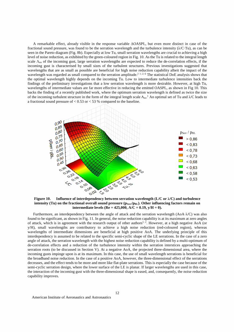
A remarkable effect, already visible in the response variable ΔOASPL, but even more distinct in case of the fractional sound pressure, was found to be the serration wavelength and the turbulence intensity (λ/C·Tu), as can be seen in the Pareto diagram (Fig. 8b). Especially at low Tu, small serration wavelengths are crucial to achieving a high level of noise reduction, as exhibited by the green-coloured region in Fig. 10. As the Tu is related to the integral length scale Λuu of the incoming gust, large serration wavelengths are expected to reduce the de-correlation effects, if the incoming gust is characterised by small sizes of the turbulent structures. Previous investigations suggested that wavelengths that are as small as possible are beneficial for high noise reduction capability albeit the impact of the wavelength was regarded as small compared to the serration amplitude.2 1; 2; 6 The statistical DoE analysis shows that the optimal wavelength highly depends on the incoming Tu. Low to intermediate turbulence intensities back the findings of the preliminary investigations that a low serration wavelength is more desirable. However, at high Tu, wavelengths of intermediate values are far more effective in reducing the emitted OASPL, as shown in Fig 10. This backs the finding of a recently published work, where the optimum serration wavelength is defined as twice the size of the incoming turbulent structure in the form of the integral length scale Λuu.1 An optimal set of Tu and λ/C leads to a fractional sound pressure of < 0.53 or < 53 % compared to the baseline.

Figure 10. Influence of interdependency between serration wavelength (L/C or λ/C) and turbulence intensity (Tu) on the fractional overall sound pressure (pSerr/pBL). Other influencing factors remain on

intermediate levels (Re = 425,000, A/C = 0.19, y/H = 0).

Furthermore, an interdependency between the angle of attack and the serration wavelength (AoA·λ/C) was also found to be significant, as shown in Fig. 11. In general, the noise reduction capability is at its maximum at zero angles of attack, which is in agreement with the research output of other authors1; 2. However, at a high negative AoA (or y/H), small wavelengths are contributory to achieve a high noise reduction (red-coloured region), whereas wavelengths of intermediate dimensions are beneficial at high positive AoA. The underlying principle of this interdependency is assumed to be related to the specific semi-cyclic shape of the LE serrations. In the case of a zero angle of attack, the serration wavelength with the highest noise reduction capability is defined by a multi-optimum of de-correlation effects and a reduction of the turbulence intensity within the serration interstices approaching the serration roots (to be discussed in Section V). At a negative AoA, the projected three-dimensional area, where the incoming gusts impinge upon is at its maximum. In this case, the use of small wavelength serrations is beneficial for the broadband noise reduction. In the case of a positive AoA, however, the three-dimensional effect of the serrations decreases, and the effect tends to be more and more like flat-plate serrations. This is especially the case because of the semi-cyclic serration design, where the lower surface of the LE is planar. If larger wavelengths are used in this case, the interaction of the incoming gust with the three-dimensional shape is eased, and, consequently, the noise reduction capability improves.

pSerr / pBL


13

Figure 11. Response variable of overall sound pressure level reduction (ΔOASPL). Influence of

interdependency between wavelength/angle of attack (λ/C · y/H). Other factors remain on intermediate levels (Re = 425,000, Tu = 3.8 %, A/C = 0.19).

Generally, as shown in Fig. 12a, the serration amplitude is the main factor in reducing the broadband noise, which is mainly effective in a frequency range of 850 Hz to 3500 Hz, where an average effect on the local SPL reduction of up to ΔSPL ≈ 10 dB is achieved by the largest serration amplitude (A/C = 0.3).

Independently, the turbulence intensity was found to be another important factor for the level of broadband noise reduction. The narrow band spectra of three representative measurement trials at intermediate settings of the remaining factors are plotted in Fig. 12b. It can be seen that the difference between the emitted noise of the baseline and the serration increases with increasing Tu. This effect is especially distinct in the intermediate frequency range of approximately 800 Hz to 4 kHz. It is important to note that the frequency range, where a sound reduction takes place, broadens with a rising turbulence intensity. Altering the Tu from low to intermediate values causes an increase of the upper frequency limit, where high turbulence intensities lead a decrease of the low frequency limit. The broadband noise emissions and thus the OASPL rise with an increase of the turbulence intensity. Consequently, the noise reduction capabilities of serrated LE are most effective at these conditions.

Figure 12. Emitted aerofoil leading edge broadband noise. Other influencing parameters remain on intermediate levels. a) different serration amplitudes (A/C), where vertical dashed lines indicate major

bandwidth of noise reduction (850 Hz < f < 3.5 kHz). b) Variation of the Tu. Baseline (straight) and serrated LE (semicolon) measurements. Offset shifted by 0 dB, 15 dB and 30 dB respectively.

In order to compare the measurement results to the theory, Amiets36 flat plate approach was used for selected configurations of the baseline case to predict the leading edge far-field sound pressure level of a flat plate exposed to a turbulent flow.

ΔOASPL [dB]

b) a)


14

Analysis of the measurements with a straight LE (baseline case) yielded a scaling of the emitted noise with the 2nd power of the turbulence intensity and the 4th power of the free stream velocity or the Mach number, respectively. Slightly deviant results were achieved by analysing the emitted OASPL of serrated LE. Amiet’s36 model was modified according to the scaling of the Mach number for the NACA65(12)-10 aerofoil, and by taking into account Gershfeld’s37 modification to consider the aerofoil thickness. Equation 15 gives:

j`�5�mnop = 10 log � �! G2�∙8�� K ��∙��9 L�� ∙ -�� G0b��9K�� + 181.3� (15)

where Λuu is the longitudinal integral length scale of the turbulence, R the observer distance, h the aerofoil semispan, z the thickness and �� the normalised chordwise wavenumber. Integral length scale and turbulence intensity were measured independently of the noise, and represent aerodynamic parameters of the flow. The model takes into account the cross power spectral density of the surface pressure on the aerofoil caused by turbulence. This can be described via the energy spectrum of the turbulence intensity (Fig. 2).

The comparison of the noise spectral density for the baseline case (straight LE) shows a good agreement with Amiet’s flat plate model in the case of intermediate parameter settings, as shown in Fig. 13. At extreme settings of the parameters, however, the comparison between the emitted noise and Amiet’s model is less accurate.

Figure 13. 1/3 Octave band spectrum. Verification of Amiet’s adopted flat plate model, taking into account

the aerofoil thickness acc. to Gershfeld.36; 37 Theoretical results (diamond, red) vs. measurements (circle, black). Tu = 3.8 %, y/H = 0, Re = 425,000, Λuu = 5.8 mm. Additional plot of measured narrow band spectrum.

B. Model Refinement Complementary measurements were carried out in the outer regions of the defined experimental space to test the

stability of the statistical model, especially at extreme settings of the influencing parameters. The measurement results were found to fit well into the model, although an increase of prediction uncertainty was observed with multiple factors on extreme levels, which statistically represents a large distance between the central point and the measurement locations. In general, the model was found to predict the noise emissions and the noise reduction reasonably accurate.

However, up to now, the model bases on a data basis of 59 measurement trials, including the measurement of the central point for 17 times to describe the statistical spread. The stability of the model, could be improved by incorporating additional data points from a previous study, which took place under the same measurement conditions, but with different leading edges and flow parameters.2 For this purpose, trials of the executed measurements as well as the results of the validation measurements were added to the existing model. 285 measurement results for the emitted noise of serrated LE at various configurations, and the noise reduction by comparison to the baseline cases were implemented. The additional measurement results are based on eight serration designs (Fig. 14b), which were tested in a velocity range of 20 ms-1 ≤ U0 ≤ 60 ms-1, or Reynolds number of 200,000 ≤ Re ≤ 600,000 respectively. The turbulence was varied by using three grids with different mesh dimensions, yielding Tu = 3.2 %, 3.7 % and 5.5 %. The angle of attack was altered from -0.102 ≤ y/H ≤ 0.128. The extra data points are also found to fit well to the regression curve (Fig. 14a), and the fit of regression shows a match of high order, when comparing the observed and predicted values in the case of the emitted OASPL for the serrated LE.

0

10

20

30

40

50

60

70

80

90

200 4000

SP

L,

dB

f, Hz

Measurement; 84.8 dB

Model Amiet; 84.6 dB

Measured narrow band


15

Figure 14. a) Incorporated data points to initial model as shown in Fig. 7. Check of model validity for serrated LE noise (OASPLSerr). b) Test matrix of additional data points from previous study at 200,000 ≤ Re ≤

600,000 and -0.102 ≤ y/H ≤ 0.128.2

Comparing the initially defined model with the refined one results in dependencies of the same order and magnitude in case of the emitted noise and noise reduction. Compared to Fig. 15a, the modified interdependency plot between Re and λ/C for the OASPL of serrated aerofoil (Fig 15b) remains almost unaffected by the additional amount of data points, but is much more reliable by now due to the increased data pool.

Figure 15. Comparison of interdependency between Reynolds number and serration wavelength (Re · λ/C). Original model a) and adapted model b) by use of additional data points (circles).2

To conclude, the influence of the additional data pool on the main factors is of negligible impact. Furthermore, all interdependencies show a constant behaviour only with slight changes in magnitude due to the additional data. This comparison implies that the initially developed statistical-empirical model is stable and reliable.

Observed vs. predicted values5 Factors, 1 Block, 343 Runs; MQ abs. error = 0.0180896

AV OASPL_Serr

55 60 65 70 75 80 85 90 95

Observed OASPL_Serr, dB

50

55

60

65

70

75

80

85

90

95

Pre

dict

ed O

AS

PL_

Ser

r, d

B A [mm] 30 45

λ [m

m] 7.5 x x

15 x x 30 x x 45 x x

b)

a)

a) b)


16

C. Model Validation with External Data To validate the current statistical-empirical model, the predicted broadband noise reduction is compared with the

experimental results obtained independently in the DARP Aeroacoustic Wind Tunnel at the Institute of Sound and Vibration Research, University of Southampton.1 The model was scaled in accordance with the changing boundary conditions and the predicted values were compared to the experimental data. The aerofoil used in Southampton is the same (NACA 65(12)-10) with a chord length C = 150 mm and a span of S = 450 mm. To prevent tonal noise generation due to the convection of Tollmien Schlichting waves in the laminar boundary layer, they tripped the flow near the leading edge at both the suction and the pressure side to force a transition to a turbulent flow. Nevertheless the tripping can be assumed to have no influence on the leading edge noise.38; 39. The tests were performed by the use of serrated sinusoidal leading edges, defined by the amplitude, with a peak-to-trough ratio of 2h and the wavelength λ. An important difference to the aerofoil used in the Southampton study is the fact that the serration peak extends the initial aerofoil chord length by 1h, giving an averaged-chord comparable to that of the baseline leading edge. The turbulence intensities were generated at Tu = 2.5 % and 3.2 %, and the incoming flow velocity U0= 20 ms-1, 40 ms-1 and 60 ms-1. The distance of the microphone location in order to measure the far-field noise was different as well, and could be corrected by use of the monopole scaling law according to Eq. 16.

j`�(n�) = j`�(n0) − �20 ∙ CVq G�5�9K� → ~j`� = �20 ∙ CVq G�5�9K� (16)

where d1 and d2 are the absolute distances between the source and the observer (measurement location) at a polar angle of Θ = 90 deg. Differences in the span were compensated by a linear scaling as well. Twelve measurement points were analysed at zero angles of attack and Tu = 2.5 %. The free stream velocity was set to U0 = 40 ms-1 and U0 = 60 ms-1, while the serration amplitude and the wavelength were varied on three levels each (Fig. 16).

Applying the specific boundary conditions of the test rig to the current model yields predictions of the OASPL with the baseline and the serrations that exhibit excellent agreement with the measurement data presented in Fig. 16. The overall noise reduction ΔOASPL demonstrated a good agreement with the predictions, although with a slightly larger error margins.

Figure 16. Validation of the current statistical-empirical model with external experimental data provided

by ISVR, University of Southampton.1 Analysis of the predicted OASPL with serrated LE (straight) and OASPL reduction (ΔOASPL, dotted). Circle and cross indicate the ISVR experimental results. 1

The emitted noise level reduces with an increase of the serration amplitude, as predicted by the model, even though the influence of the wavelength shows a deviant behaviour. The comparative data underlines a decreasing OASPL with increasing wavelength, which contradicts the findings and affects the fit of the model. This trend accumulates regarding the overall noise reduction. The divergence between predicted and measured value is up to 1.2 dB at the highest wavelength. Altogether, the current statistical model can be regarded as a robust tool for the predictions of the AGI broadband noise subjected to serrated LEs.

0

5

10

15

20

40

50

60

70

80

90

100

110

0,1 0,2 0,3 0,4

dO

AS

PL,

dB

OA

SP

L, d

B

A/C

Exp Re = 394,188 Exp Re = 624,348Predict Re = 394,188 Predict Re = 624,348

0

5

10

15

20

40

50

60

70

80

90

100

110

0,1 0,1 0,2 0,2 0,3dO

AS

PL,

dB

OA

SP

L, d

B

λ/C

Exp Re = 394,188 Exp Re = 624,348Predict Re = 394,188 Predict Re = 624,348


17

V. Aerodynamic Results Up to now, there is little experimentally based information in the literature to describe the effect of serration

parameters on the flow in front of and within the interstices of the serrated Les. Therefore, little is known about the flow field within the serrations, which has the potential to be the main acoustic source for the leading edge noise. In the following, some results of the experimental PIV study are presented with the aim to describe the patterns of the flow approaching the leading edge, the flow within the serrations and the turbulence of various serration geometries at different streamwise locations. In principle, the incoming turbulence causes surface pressure fluctuation on the aerofoil LE that acts as main mechanism to radiate broadband noise. Serrated LEs result in incoherent response times of the surface to the incident turbulence across the span.6 This results in a decreased level of surface pressure fluctuation and ultimately a reduced level of broadband noise. Because the changes in the flow field within the serration have a potential to influence the incident pressure fluctuation, the scattering mechanism might also be affected which ultimately causes a reduction in the broadband noise5. Hence, an improved understanding of the underlying principles can be obtained by a detailed study of the flow field at regions close to the LE serration.

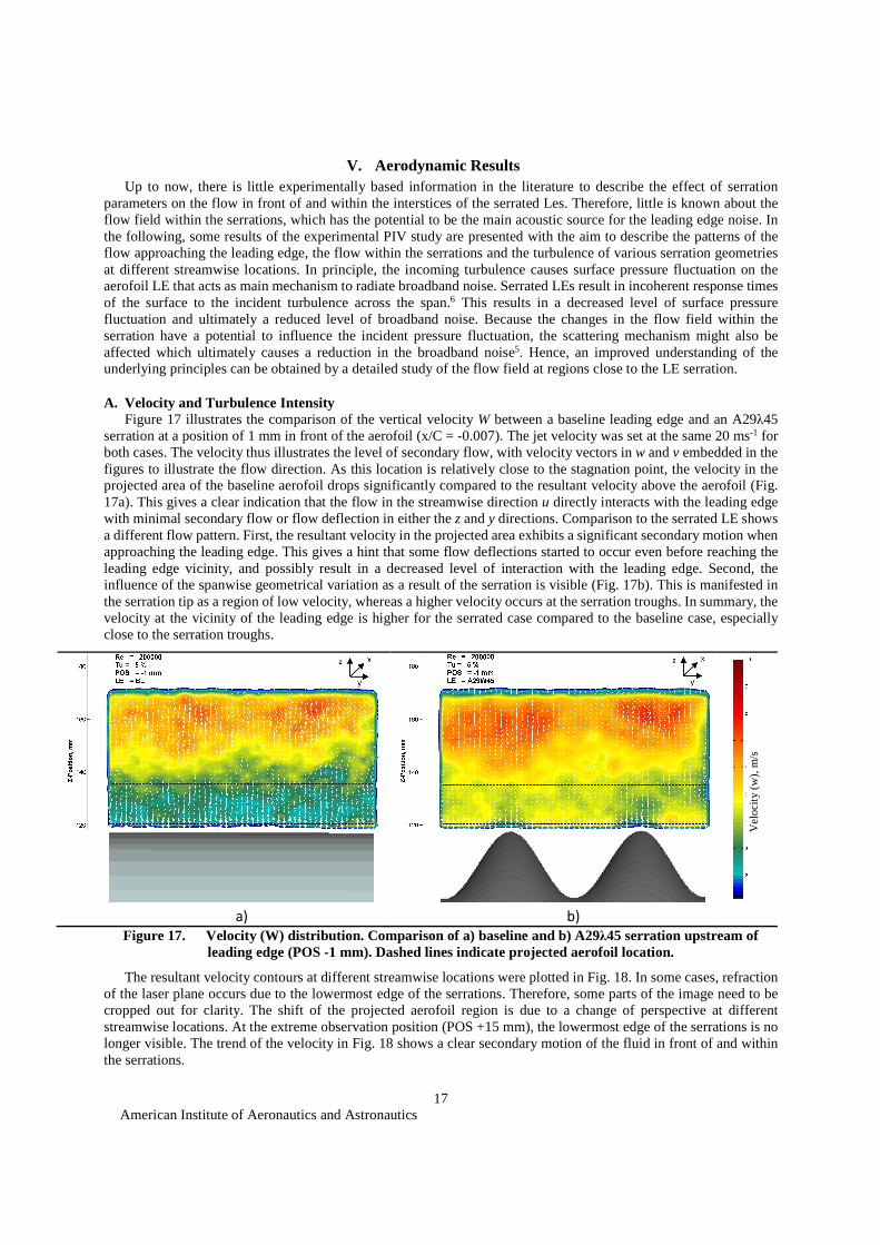
A. Velocity and Turbulence Intensity Figure 17 illustrates the comparison of the vertical velocity W between a baseline leading edge and an A29λ45

serration at a position of 1 mm in front of the aerofoil (x/C = -0.007). The jet velocity was set at the same 20 ms-1 for both cases. The velocity thus illustrates the level of secondary flow, with velocity vectors in w and v embedded in the figures to illustrate the flow direction. As this location is relatively close to the stagnation point, the velocity in the projected area of the baseline aerofoil drops significantly compared to the resultant velocity above the aerofoil (Fig. 17a). This gives a clear indication that the flow in the streamwise direction u directly interacts with the leading edge with minimal secondary flow or flow deflection in either the z and y directions. Comparison to the serrated LE shows a different flow pattern. First, the resultant velocity in the projected area exhibits a significant secondary motion when approaching the leading edge. This gives a hint that some flow deflections started to occur even before reaching the leading edge vicinity, and possibly result in a decreased level of interaction with the leading edge. Second, the influence of the spanwise geometrical variation as a result of the serration is visible (Fig. 17b). This is manifested in the serration tip as a region of low velocity, whereas a higher velocity occurs at the serration troughs. In summary, the velocity at the vicinity of the leading edge is higher for the serrated case compared to the baseline case, especially close to the serration troughs.

a) b)

Figure 17. Velocity (W) distribution. Comparison of a) baseline and b) A29λ45 serration upstream of leading edge (POS -1 mm). Dashed lines indicate projected aerofoil location.

The resultant velocity contours at different streamwise locations were plotted in Fig. 18. In some cases, refraction of the laser plane occurs due to the lowermost edge of the serrations. Therefore, some parts of the image need to be cropped out for clarity. The shift of the projected aerofoil region is due to a change of perspective at different streamwise locations. At the extreme observation position (POS +15 mm), the lowermost edge of the serrations is no longer visible. The trend of the velocity in Fig. 18 shows a clear secondary motion of the fluid in front of and within the serrations.

Vel

ocity

(w

), m

/s


18

After first entering the serration interstices (POS +2 mm), the main peak of the velocity is well beneath the LE tip, indicated by the dashed lines. Increasing the streamwise position within the serration shows a shift of the main peak upwards towards the suction side. The closer the plane is to the serration root, the higher is the influence of the serration on the fluid above the aerofoil. The results present that the region of high velocity (i.e. secondary flow) tends to expand outwards. The velocity plots also indicate that the absolute magnitude increases with the streamwise distance. This is probably due to the tendency of flow to be accelerated either upward to downward away from the serration, thus avoiding large-scale impingement to the serration root. Ultimately, both the incident surface pressure fluctuation and the scattered pressure will be reduced, resulting in broadband noise reduction. This could be the main mechanism of the noise reduction by serration. The serrations have been shown to cause a rapid change in the velocity field. It is also of interest to examine the change in turbulence intensity. As the trend of the Tu(w) along different locations in Fig. 19 exemplifies, the Tu fairly describes the counterpart of the mean velocity.

Figure 18. Trend of vertical velocity distribution w along different streamwise locations by use of an A/C =

0.3, λ/C=0.175 (A45λ26) leading edge. Re = 200,000, Tu = 5.5 %, y/H = 0.

Figure 19. Trend of vertical turbulence intensity Tu(w) along different streamwise locations by use of A/C

= 0.3, λ/C = 0.175 (A45λ26) leading edge. Tu = 5.5 %, Re = 200,000, y/H = 0.

Vel

oci

ty (W

), m

/s

Tu(

w),

--


19

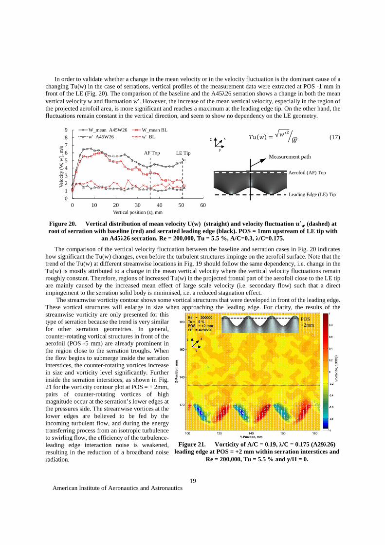
In order to validate whether a change in the mean velocity or in the velocity fluctuation is the dominant cause of a

changing Tu(w) in the case of serrations, vertical profiles of the measurement data were extracted at POS -1 mm in front of the LE (Fig. 20). The comparison of the baseline and the A45λ26 serration shows a change in both the mean vertical velocity w and fluctuation w′. However, the increase of the mean vertical velocity, especially in the region of the projected aerofoil area, is more significant and reaches a maximum at the leading edge tip. On the other hand, the fluctuations remain constant in the vertical direction, and seem to show no dependency on the LE geometry.

Figure 20. Vertical distribution of mean velocity U(w) (straight) and velocity fluctuation �� (dashed) at root of serration with baseline (red) and serrated leading edge (black). POS = 1mm upstream of LE tip with

an A45λ26 serration. Re = 200,000, Tu = 5.5 %, A/C=0.3, λ/C=0.175.

The comparison of the vertical velocity fluctuation between the baseline and serration cases in Fig. 20 indicates how significant the Tu(w) changes, even before the turbulent structures impinge on the aerofoil surface. Note that the trend of the Tu(w) at different streamwise locations in Fig. 19 should follow the same dependency, i.e. change in the Tu(w) is mostly attributed to a change in the mean vertical velocity where the vertical velocity fluctuations remain roughly constant. Therefore, regions of increased Tu(w) in the projected frontal part of the aerofoil close to the LE tip are mainly caused by the increased mean effect of large scale velocity (i.e. secondary flow) such that a direct impingement to the serration solid body is minimised, i.e. a reduced stagnation effect.

The streamwise vorticity contour shows some vortical structures that were developed in front of the leading edge. These vortical structures will enlarge in size when approaching the leading edge. For clarity, the results of the streamwise vorticity are only presented for this type of serration because the trend is very similar for other serration geometries. In general, counter-rotating vortical structures in front of the aerofoil (POS -5 mm) are already prominent in the region close to the serration troughs. When the flow begins to submerge inside the serration interstices, the counter-rotating vortices increase in size and vorticity level significantly. Further inside the serration interstices, as shown in Fig. 21 for the vorticity contour plot at POS = + 2mm, pairs of counter-rotating vortices of high magnitude occur at the serration’s lower edges at the pressures side. The streamwise vortices at the lower edges are believed to be fed by the incoming turbulent flow, and during the energy transferring process from an isotropic turbulence to swirling flow, the efficiency of the turbulence-leading edge interaction noise is weakened, resulting in the reduction of a broadband noise radiation.

0123456789

0 10 20 30 40 50 60

Velo

city

(W

, w

' ), m

/s

Vertical position (z), mm

W_mean A45W26 W_mean BLw' A45W26 w' BL -�(?) = .? �� >/* (17)

Figure 21. Vorticity of A/C = 0.19, λ/C = 0.175 (A29λ26) leading edge at POS = +2 mm within serration interstices and

Re = 200,000, Tu = 5.5 % and y/H = 0.

LE Tip AF Top Measurement path

Leading Edge (LE) Tip

POS +2mm

Aerofoil (AF) Top


20

The results in Fig. 21 correlate quite well with a numerical work5, where a spanwise secondary flow from the serration peak to the trough was observed by analysing the mean wall shear stress distribution of an aerofoil suction side.

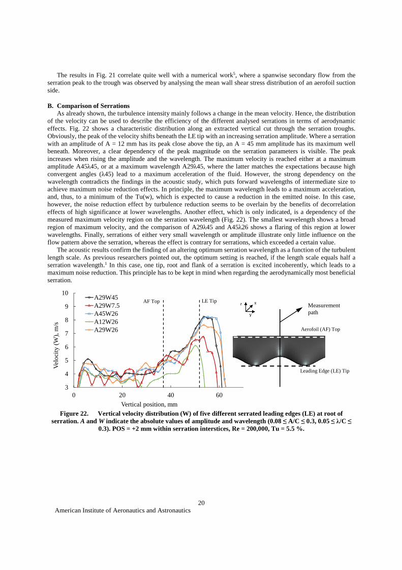
B. Comparison of Serrations As already shown, the turbulence intensity mainly follows a change in the mean velocity. Hence, the distribution

of the velocity can be used to describe the efficiency of the different analysed serrations in terms of aerodynamic effects. Fig. 22 shows a characteristic distribution along an extracted vertical cut through the serration troughs. Obviously, the peak of the velocity shifts beneath the LE tip with an increasing serration amplitude. Where a serration with an amplitude of A = 12 mm has its peak close above the tip, an A = 45 mm amplitude has its maximum well beneath. Moreover, a clear dependency of the peak magnitude on the serration parameters is visible. The peak increases when rising the amplitude and the wavelength. The maximum velocity is reached either at a maximum amplitude A45λ45, or at a maximum wavelength A29λ45, where the latter matches the expectations because high convergent angles (λ45) lead to a maximum acceleration of the fluid. However, the strong dependency on the wavelength contradicts the findings in the acoustic study, which puts forward wavelengths of intermediate size to achieve maximum noise reduction effects. In principle, the maximum wavelength leads to a maximum acceleration, and, thus, to a minimum of the Tu(w), which is expected to cause a reduction in the emitted noise. In this case, however, the noise reduction effect by turbulence reduction seems to be overlain by the benefits of decorrelation effects of high significance at lower wavelengths. Another effect, which is only indicated, is a dependency of the measured maximum velocity region on the serration wavelength (Fig. 22). The smallest wavelength shows a broad region of maximum velocity, and the comparison of A29λ45 and A45λ26 shows a flaring of this region at lower wavelengths. Finally, serrations of either very small wavelength or amplitude illustrate only little influence on the flow pattern above the serration, whereas the effect is contrary for serrations, which exceeded a certain value.

The acoustic results confirm the finding of an altering optimum serration wavelength as a function of the turbulent length scale. As previous researchers pointed out, the optimum setting is reached, if the length scale equals half a serration wavelength.1 In this case, one tip, root and flank of a serration is excited incoherently, which leads to a maximum noise reduction. This principle has to be kept in mind when regarding the aerodynamically most beneficial serration.

Figure 22. Vertical velocity distribution (W) of five different serrated leading edges (LE) at root of

serration. A and W indicate the absolute values of amplitude and wavelength (0.08 ≤ A/C ≤ 0.3, 0.05 ≤ λ/C ≤ 0.3). POS = +2 mm within serration interstices, Re = 200,000, Tu = 5.5 %.

3

4

5

6

7

8

9

10

0 20 40 60

Velo

city

(W

), m

/s

Vertical position, mm

A29W45A29W7.5A45W26A12W26A29W26

LE Tip AF Top Measurement path

Leading Edge (LE) Tip

Aerofoil (AF) Top


21

VI. Conclusion An experimental aeroacoustic study was performed in order to quantify the effects of five influencing parameters

on the broadband noise emissions and reduction of a NACA65(12)-10 aerofoil with serrated leading edges. The statistical-empirical modelling technique Design of Experiments (DoE) was utilised to reduce the experimental volume to a manageable amount in order to gain information on interdependencies of each influencing parameter and to develop a prediction tool that describes the overall noise radiation. The model, based on solely 59 measurement points, was validated and stabilised by extensive additive data. It shows a reasonably accurate performance at settings close to the defined central point of the experimental space, and only slightly less accurate predictions in the outer regions of the pre-defined setting ranges. When the predicted results are compared with external experimental data, the excellent agreement indicates that a robust and reliable statistical-empirical model was developed in this study. The aeroacoustic study was supplemented by Particle Image Velocimetry (PIV) experiments to gain insight of the flow behaviour when in close proximity or inside the serration. The aeroacoustic and aerodynamic results allow the current paper to reach the following conclusions:

- A clear ranking and quantification of the influencing parameters, where the Reynolds number (Re) and the freestream flow turbulence intensity (Tu) are the main contributors to the broadband noise emissions. The serration amplitude (A/C), followed by the Reynolds number and the serration wavelength (λ/C) represent the main factors for an effective broadband noise reduction.

- Identification of a significant interdependence of the serration wavelength and the freestream turbulence intensity (λ/C·Tu) with regard to the overall noise reduction capability. This feature could be linked to the characteristic size of the incoming gust in conjunction with a maximum phase shift.

- Identification of a significant interdependence of the angle of attack and the serration wavelength (y/H·λ/C) with regard to the overall noise reduction capability. This characteristic behaviour could be assigned to three-dimensional effects when the flow is approaching the aerofoil.

- The effect of the stagnation point on the flow in front of the leading edge was observed to reduce drastically in the case of serrations. With an advancing streamwise position along the interstices of the serrations, the velocity (i.e. secondary flow) becomes more prominent, whilst the turbulence intensity reduces. This is regarded as the main mechanism for the reduction in broadband noise because the main flow is deflected away from the stagnation point near the serration troughs.

- The analysis of the mean vertical velocity and the vertical velocity fluctuations within the interstices of the serrations reveals that changes in the mean vertical velocity dominate the turbulence intensity Tu(w).

- Counter-rotating vortices could be visualised. These streamwise vortices at the lower edges of the pressure side are believed to be fed by the incoming turbulent flow and during the energy transferring process from an isotropic turbulence to a swirling flow. Consequently, the efficiency of turbulence leading-edge interaction noise is weakened, resulting in the reduction of broadband noise radiation.

- The serration amplitude has been confirmed as the dominant parameter for the reduction of the broadband noise. In the case of the serration wavelength, a contradicting behaviour between the aerodynamic and aeroacoustic performances is observed

- It was found that a small or intermediate wavelength reduces the broadband noise more effectively than large wavelengths, which is backed by the hypothesis that the origin of the noise reduction mechanism, due to serrations, is not solely of an aerodynamic but also of an acoustic nature. The noise reduction principle of strong incoherent effects at small to intermediate wavelengths superimposes the effect of a high Tu reduction with large wavelengths.


22

References 1Chaitanya, P., Narayanan, S., Joseph, P., Vanderwel, C., Kim, J. W., et al., “Broadband noise reduction

through leading edge serrations on realistic aerofoils,” 21st AIAA/CEAS Aeroacoustics Conference, 2015. 2Chong, T. P., Vathylakis, A., McEwen, A., Kemsley, F., Muhammad, C., et al., “Aeroacoustic and

Aerodynamic Performances of an Aerofoil Subjected to Sinusoidal Leading Edges,” 21st AIAA/CEAS Aeroacoustics Conference, 2015.

3Hersh, A. S., Sodermant, P. T., and Hayden, R. E., “Investigation of Acoustic Effects of Leading-Edge Serrations on Airfoils,” Journal of Aircraft, Vol. 11, No. 4, 1974, pp. 197–202.

4Narayanan, S., Chaitanya, P., Haeri, S., Joseph, P., Kim, J. W., et al., “Airfoil noise reductions through leading edge serrations,” Physics of Fluids, Vol. 27, No. 2, 2015, p. 25109.

5Chen, W., Qiao, W., Wang, L., Tong, F., and Wang, X., “Rod-Airfoil Interaction Noise Reduction Using Leading Edge Serrations,” 21st AIAA/CEAS Aeroacoustics Conference, 2015.

6Lau, A. S., Haeri, S., and Kim, J. W., “The effect of wavy leading edges on aerofoil–gust interaction noise,” Journal of Sound and Vibration, Vol. 332, No. 24, 2013, pp. 6234–6253.

7Custodio, D., “The Effect of Humpback Whale-like Leading Edge Protuberances on Hydrofoil Performance,” Master Dissertation, Worcester Polytechnic Institute, Worcester, USA, December 2007.

8Melo De Sousa, J., and Camara, J., “Numerical Study on the Use of a Sinusoidal Leading Edge for Passive Stall Control at Low Reynolds Number,” 51st AIAA Aerospace Sciences Meeting including the New Horizons Forum and Aerospace Exposition.

9Gawad, A. F., “Utilization of Whale-Inspired Tubercles as a ControlTechnique to Improve Airfoil Performance,” Transaction on Control and Mech. Systems, Vol. 2, No. 5, 2013, pp. 212–218.

10Paterson, R. W., and Amiet, R. K., “Acoustic Radiation and Surface Pressure Characteristics of an Airfoil due to Incident Turbulence,” NASA CR-2733, September 1976.

11Staubs, J. K., “Real Airfoil Effects on Leading Edge Noise,” Ph.D. Dissertation, Faculty of the Virginia Polytechnic Institute, Blacksburg, USA, May 2008.

12Collins, F. G., “Boundary-Layer Control on Wings Using Sound and Leading-Edge Serrations,” AIAA Journal, Vol. 19, No. 2, 1981, pp. 129–130.

13Fish, F. E., and Battle, J. M., “Hydrodynamic Design of the Humpback Whale Flipper,” Journal of Morphology, Vol. 1995, No. 225, 1995, pp. 51–60.

14Soderman, P. T., “Aerodynamic Effects of Leading-Edge Serrations on a Two-Dimensional Airfoil,” NASA TM X-2643, September 1972.

15Biedermann, T., “Aerofoil noise subjected to leading edgeserration,” Master Dissertation, Institute of Sound and Vibration Engineering ISAVE, Düsseldorf, September 2015.

16McEwen, A., “Aerofoil Noise Reduction by Leading Edge Tubercles,” Graduate project, Department of Mechanical, Aerospace and Civil Engineering, London, UK, 2015.

17Chong, T. P., Joseph, P. F., and Davies, P., “Design and performance of an open jet wind tunnel for aero-acoustic measurement,” Applied Acoustics, Vol. 70, No. 4, 2009, pp. 605–614.

18Laws, E. M., and Livesey, J. L., “Flow Through Screens,” Annual Review of Fluid Mechanics, Vol. 10, No. 1, 1978, pp. 247–266.

19Aufderheide, T., Bode, C., Friedrichs, J., and Kozulovic, D., “The Generation of Higher Levels of Turbulence in in a Low-Speed Cascade Windtunnel by Pressurized Tubes,” 11th World Congress on Computational Mechanics, Vol. 2014, 2014.

20Rozenberg, Y., “Modélisation analytique du bruit aérodynamique à largebande des machines tournantes : utilisation de calculs moyennés de mécanique des fuides,” Docteur Spécialité Acoustique Dissertation, Lyon, Frankreich, 2007.

21Vathylakis, A., Chong, T. P., and Kim, J. H., “Design of a low-noise aeroacoustic wind tunnel facility at Brunel University,” 20th AIAA/CEAS Aeroacoustics Conference.

22Raffel, M., Willert, C. E., Wereley, S. T., and Kompenhans, J., Particle Image Velocimetry. A Practical Guide, Springer, Dordrecht, 2007.

23Dantec Dynamics, Dynamic Studio, 2013. 24McMurtry, P., Vorticity Dynamics, The University of Utah, USA, 2001. 25Adam, M., Statistische Versuchsplanung und Auswertung (DoE Design of Experiments), University of

Applied Sciences Dusseldorf, Germany, 2012.


23

26Clementi, S., Fernandi, M., Baroni, M., Decastri, D., Randazzo, G. M., et al., “Mauro: A Novel Strategy for Optimizing Mixture Properties,” Applied Mathematics, Vol. 03, No. 10, 2012, pp. 1260–1264.

27Kleppmann, W., Taschenbuch Versuchsplanung. Produkte und Prozesse optimieren, 5th ed., Hanser, München, 2008.

28Haase, D., “Ein neues Verfahren zur modellbasierten Prozessoptimierung auf der Grundlage der statistischen Versuchsplanung am Beispiel eines Ottomotors mit elektromagnetischer Ventilsteuerung (EMVS),” Dr.-Ing. Dissertation, Fakultät für Verkehrswissenschaften „Friedrich List“, Dresden, 2004.

29Siebertz, K., van Bebber, D., and Hochkirchen, T., Statistische Versuchsplanung, Springer Berlin Heidelberg, Berlin, Heidelberg, 2010.

30Clair, V., Polacsek, C., Le Garrec, T., Reboul, G., Gruber, M., et al., “Experimental and Numerical Investigation of Turbulence-Airfoil Noise Reduction Using Wavy Edges,” AIAA Journal, Vol. 51, No. 11, 2013, pp. 2695–2713.

31Gruber, M., “Airfoil noise reduction by edge treatments,” Ph.D. Dissertation, Institute of Sound and Vibration Research, Southampton, UK, February 2012.

32Hansen, K. L., “Effect of Leading Edge Tubercles on Airfoil Performance,” Ph.D. Dissertation, School of Mechanical Engineering, Adelaide, Australia, July 2012.

33Narayanan, S., Joseph, P., Haeri, S., and Kim, J. W., “Noise Reduction Studies from the Leading Edge of Serrated Flat Plates,” 20th AIAA/CEAS Aeroacoustics Conference, 2014.

34Polacsek, C., Reboul, G., Clair, V., Le Garrec, T., and Deniau, H., “Turbulence-airfoil interaction noise reduction using wavy leading edge: An experimental and numerical study,” Inter Noise 2011, 2011.

35Roger, M., Schram, C., and Santana, L. de, “Reduction of Airfoil Turbulence-Impingement Noise by Means of Leading-Edge Serrations and/or Porous Material,” 19th AIAA/CEAS Aeroacoustics Conference, 2013.

36Amiet, R. K., “Acoustic Radiation from an Airfoil in a Turbulent Stream,” Journal of Sound and Vibration, Vol. 1975, 41(4), 1975, pp. 407--420.

37Gershfeld, J., “Leading Edge Noise from Thick Foils in Turbulent Flows,” NSWCCD-72-TR-2003/099, 2003.

38Geyer, T., Sarradj, E., and Giesler, J., “Application of a Beamforming Technique to the Measurement of Airfoil Leading Edge Noise,” Advances in Acoustics and Vibration, Vol. 2012, No. 3, 2012, pp. 1–16.

39Oerlemans, S., and Migliore, P., “Aeroacoustic Wind Tunnel Tests of Wind Turbine Airfoils,” 10th AIAA/CEAS Aeroacoustics Conference.

40Yang, J., Vorticity Theorems, The University of Iowa, Iowa, USA, 2012.

Statistical-Empirical Modelling of Aerofoil Noise ... · Frank Kameier 3 Duesseldorf University of...

Documents

Transcript of Statistical-Empirical Modelling of Aerofoil Noise ... · Frank Kameier 3 Duesseldorf University of...