Slides networks-tranport-2017-2-1
39
Arthur Charpentier, Master Statistique & Économétrie - Université Rennes 1 - 2017 Arthur Charpentier [email protected] https://freakonometrics.github.io/ Université Rennes 1, 2017 Graphs, Networks & Flows # 1 @freakonometrics freakonometrics freakonometrics.hypotheses.org 1
-
Upload
arthur-charpentier -
Category
Education
-
view
4.153 -
download
0
Transcript of Slides networks-tranport-2017-2-1

Arthur Charpentier, Master Statistique & Économétrie - Université Rennes 1 - 2017
Arthur [email protected]://freakonometrics.github.io/Université Rennes 1, 2017
Graphs, Networks & Flows # 1
@freakonometrics freakonometrics freakonometrics.hypotheses.org 1
Arthur Charpentier, Master Statistique & Économétrie - Université Rennes 1 - 2017
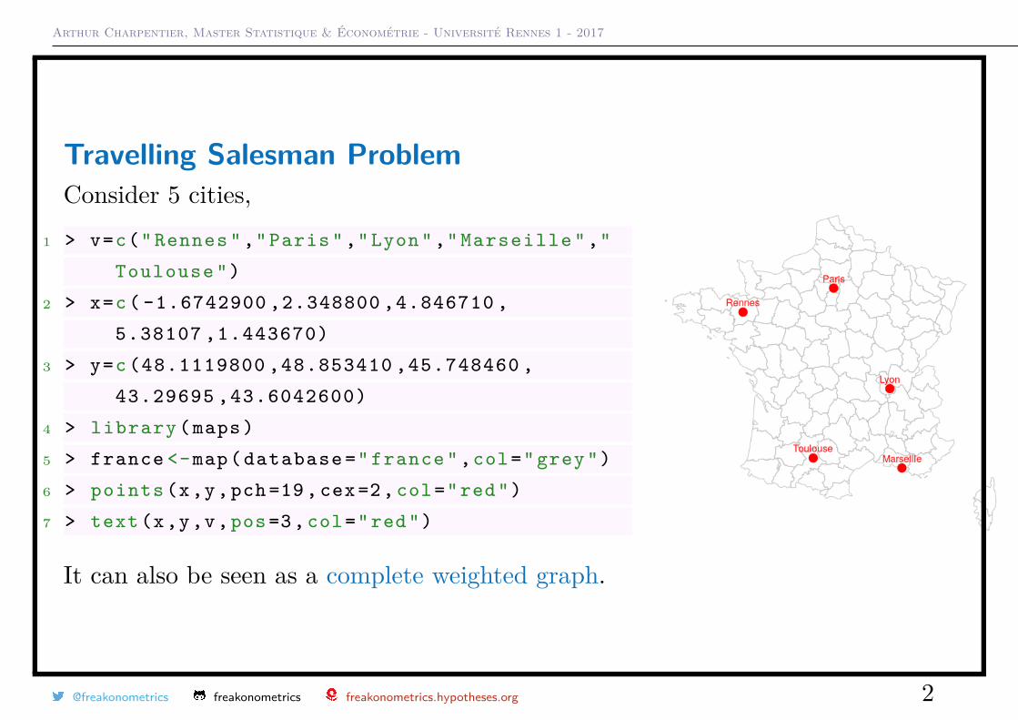
Travelling Salesman ProblemConsider 5 cities,
1 > v=c(" Rennes "," Paris ","Lyon"," Marseille ","
Toulouse ")
2 > x=c ( -1.6742900 ,2.348800 ,4.846710 ,
5.38107 ,1.443670)
3 > y=c (48.1119800 ,48.853410 ,45.748460 ,
43.29695 ,43.6042600)
4 > library (maps)
5 > france <-map( database =" france ",col="grey")
6 > points (x,y,pch =19 , cex =2, col="red")
7 > text(x,y,v,pos =3, col="red")
It can also be seen as a complete weighted graph.
@freakonometrics freakonometrics freakonometrics.hypotheses.org 2
Arthur Charpentier, Master Statistique & Économétrie - Université Rennes 1 - 2017
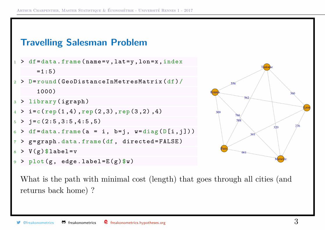
Travelling Salesman Problem
1 > df=data. frame (name=v,lat=y,lon=x, index
=1:5)
2 > D= round ( GeoDistanceInMetresMatrix (df)/
1000)
3 > library ( igraph )
4 > i=c(rep (1 ,4) ,rep (2 ,3) ,rep (3 ,2) ,4)
5 > j=c(2:5 ,3:5 ,4:5 ,5)
6 > df=data. frame (a = i, b=j, w=diag(D[i,j]))
7 > g= graph .data. frame (df , directed = FALSE )
8 > V(g)$ label =v
9 > plot(g, edge. label =E(g)$w)
What is the path with minimal cost (length) that goes through all cities (andreturns back home) ?
@freakonometrics freakonometrics freakonometrics.hypotheses.org 3
Arthur Charpentier, Master Statistique & Économétrie - Université Rennes 1 - 2017
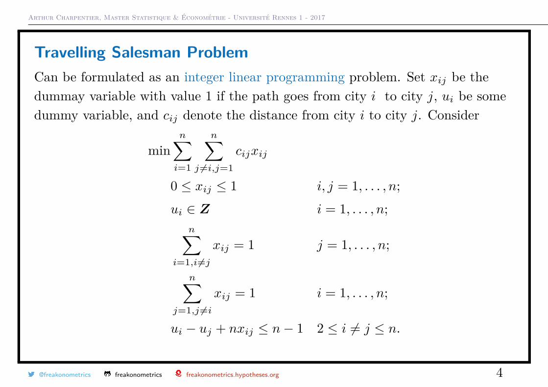
Travelling Salesman ProblemCan be formulated as an integer linear programming problem. Set xij be thedummay variable with value 1 if the path goes from city i to city j, ui be somedummy variable, and cij denote the distance from city i to city j. Consider
minn∑i=1
n∑j 6=i,j=1
cijxij
0 ≤ xij ≤ 1 i, j = 1, . . . , n;ui ∈ Z i = 1, . . . , n;
n∑i=1,i6=j
xij = 1 j = 1, . . . , n;
n∑j=1,j 6=i
xij = 1 i = 1, . . . , n;
ui − uj + nxij ≤ n− 1 2 ≤ i 6= j ≤ n.
@freakonometrics freakonometrics freakonometrics.hypotheses.org 4
Arthur Charpentier, Master Statistique & Économétrie - Université Rennes 1 - 2017
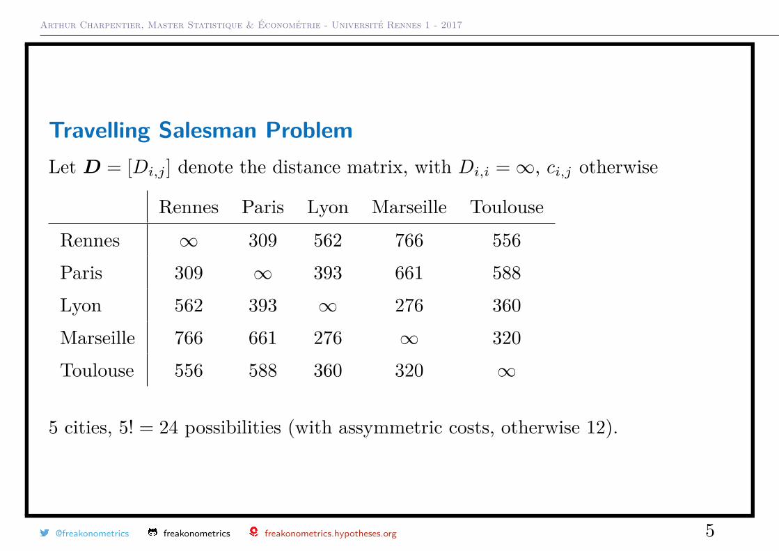
Travelling Salesman ProblemLet D = [Di,j ] denote the distance matrix, with Di,i =∞, ci,j otherwise
Rennes Paris Lyon Marseille Toulouse
Rennes ∞ 309 562 766 556Paris 309 ∞ 393 661 588Lyon 562 393 ∞ 276 360Marseille 766 661 276 ∞ 320Toulouse 556 588 360 320 ∞
5 cities, 5! = 24 possibilities (with assymmetric costs, otherwise 12).
@freakonometrics freakonometrics freakonometrics.hypotheses.org 5

Arthur Charpentier, Master Statistique & Économétrie - Université Rennes 1 - 2017
Travelling Salesman ProblemOne can use brute force search
1 > library ( combinat )
2 > M= matrix ( unlist ( permn (1:5) ),nrow =5)
3 > sM=M[,M[1 ,]==1]
4 > sM= rbind (sM ,1)
5 > traj= function (vi){
6 + s=0
7 + for(i in 1:( length (vi) -1)) s=s+D[vi[i],
vi[i+1]]
8 + return (s) }
9 > d= unlist ( lapply (1: ncol(sM),function (x)
traj(sM[,x])))
10 > sM= rbind (sM ,d)
11 > sM[, which .min(d)]
12 d
13 1 2 3 4 5 1 1854
@freakonometrics freakonometrics freakonometrics.hypotheses.org 6
Arthur Charpentier, Master Statistique & Économétrie - Université Rennes 1 - 2017
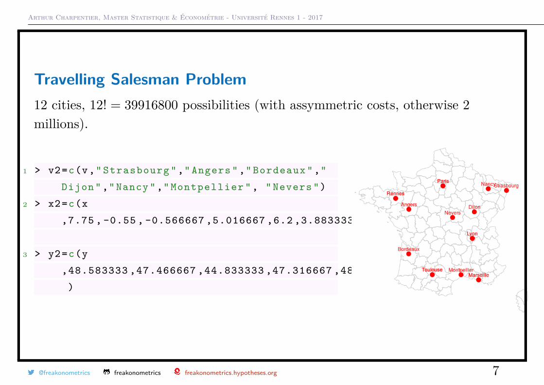
Travelling Salesman Problem12 cities, 12! = 39916800 possibilities (with assymmetric costs, otherwise 2millions).
1 > v2=c(v," Strasbourg "," Angers "," Bordeaux ","
Dijon "," Nancy "," Montpellier ", " Nevers ")
2 > x2=c(x
,7.75 , -0.55 , -0.566667 ,5.016667 ,6.2 ,3.883333 ,3.166667)
3 > y2=c(y
,48.583333 ,47.466667 ,44.833333 ,47.316667 ,48.683333 ,43.6 ,46.983333
)
@freakonometrics freakonometrics freakonometrics.hypotheses.org 7
Arthur Charpentier, Master Statistique & Économétrie - Université Rennes 1 - 2017
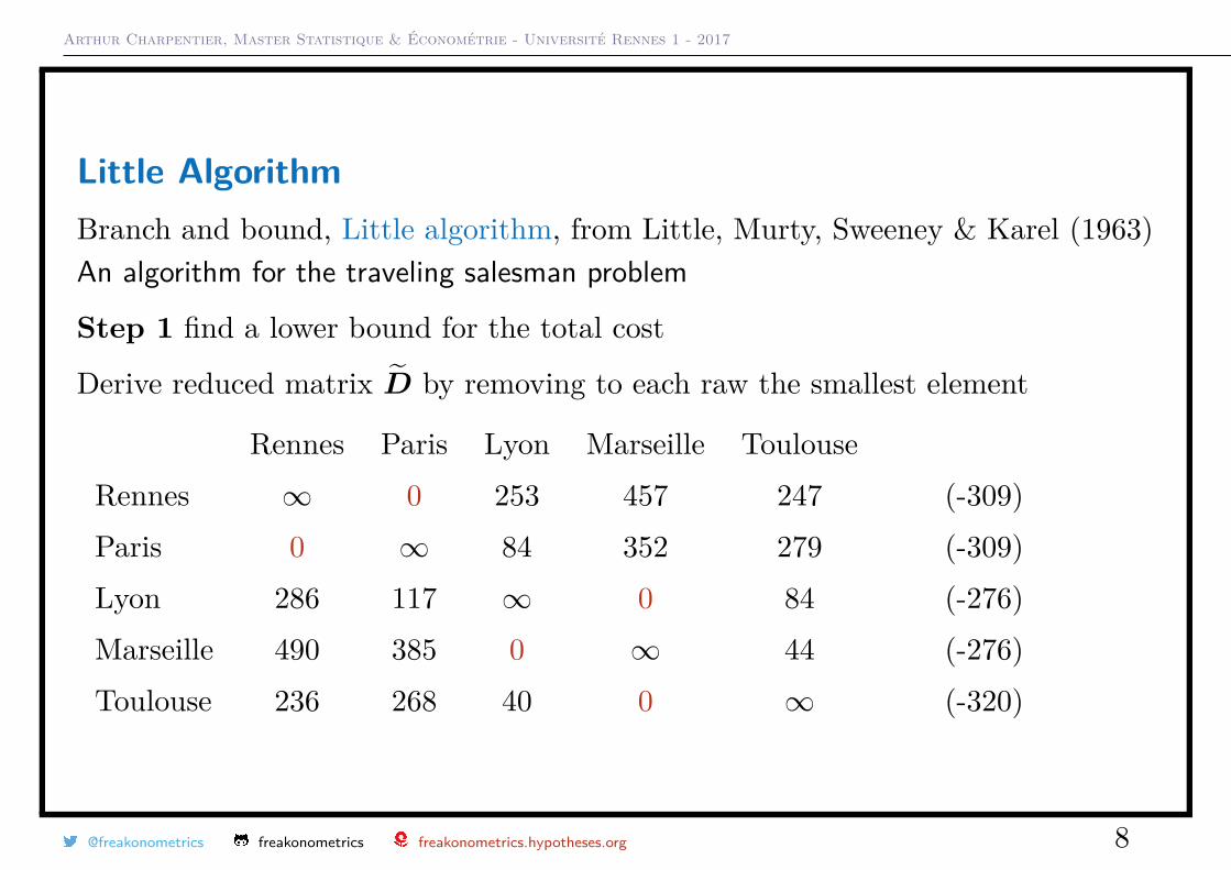
Little AlgorithmBranch and bound, Little algorithm, from Little, Murty, Sweeney & Karel (1963)An algorithm for the traveling salesman problem
Step 1 find a lower bound for the total cost
Derive reduced matrix D̃ by removing to each raw the smallest element
Rennes Paris Lyon Marseille ToulouseRennes ∞ 0 253 457 247 (-309)Paris 0 ∞ 84 352 279 (-309)Lyon 286 117 ∞ 0 84 (-276)Marseille 490 385 0 ∞ 44 (-276)Toulouse 236 268 40 0 ∞ (-320)
@freakonometrics freakonometrics freakonometrics.hypotheses.org 8
Arthur Charpentier, Master Statistique & Économétrie - Université Rennes 1 - 2017
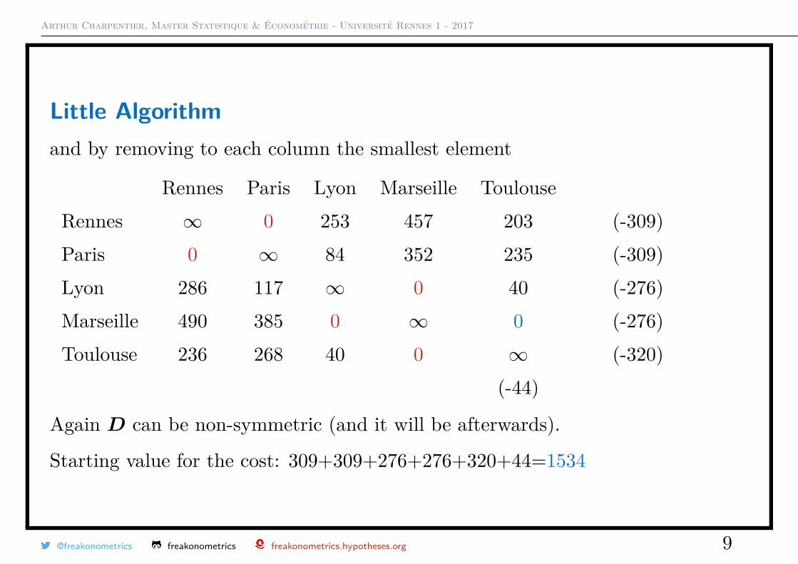
Little Algorithmand by removing to each column the smallest element
Rennes Paris Lyon Marseille ToulouseRennes ∞ 0 253 457 203 (-309)Paris 0 ∞ 84 352 235 (-309)Lyon 286 117 ∞ 0 40 (-276)Marseille 490 385 0 ∞ 0 (-276)Toulouse 236 268 40 0 ∞ (-320)
(-44)
Again D can be non-symmetric (and it will be afterwards).
Starting value for the cost: 309+309+276+276+320+44=1534
@freakonometrics freakonometrics freakonometrics.hypotheses.org 9
Arthur Charpentier, Master Statistique & Économétrie - Université Rennes 1 - 2017
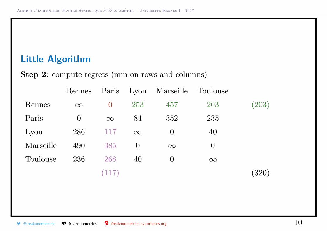
Little AlgorithmStep 2: compute regrets (min on rows and columns)
Rennes Paris Lyon Marseille ToulouseRennes ∞ 0 253 457 203 (203)Paris 0 ∞ 84 352 235Lyon 286 117 ∞ 0 40Marseille 490 385 0 ∞ 0Toulouse 236 268 40 0 ∞
(117) (320)
@freakonometrics freakonometrics freakonometrics.hypotheses.org 10
Arthur Charpentier, Master Statistique & Économétrie - Université Rennes 1 - 2017
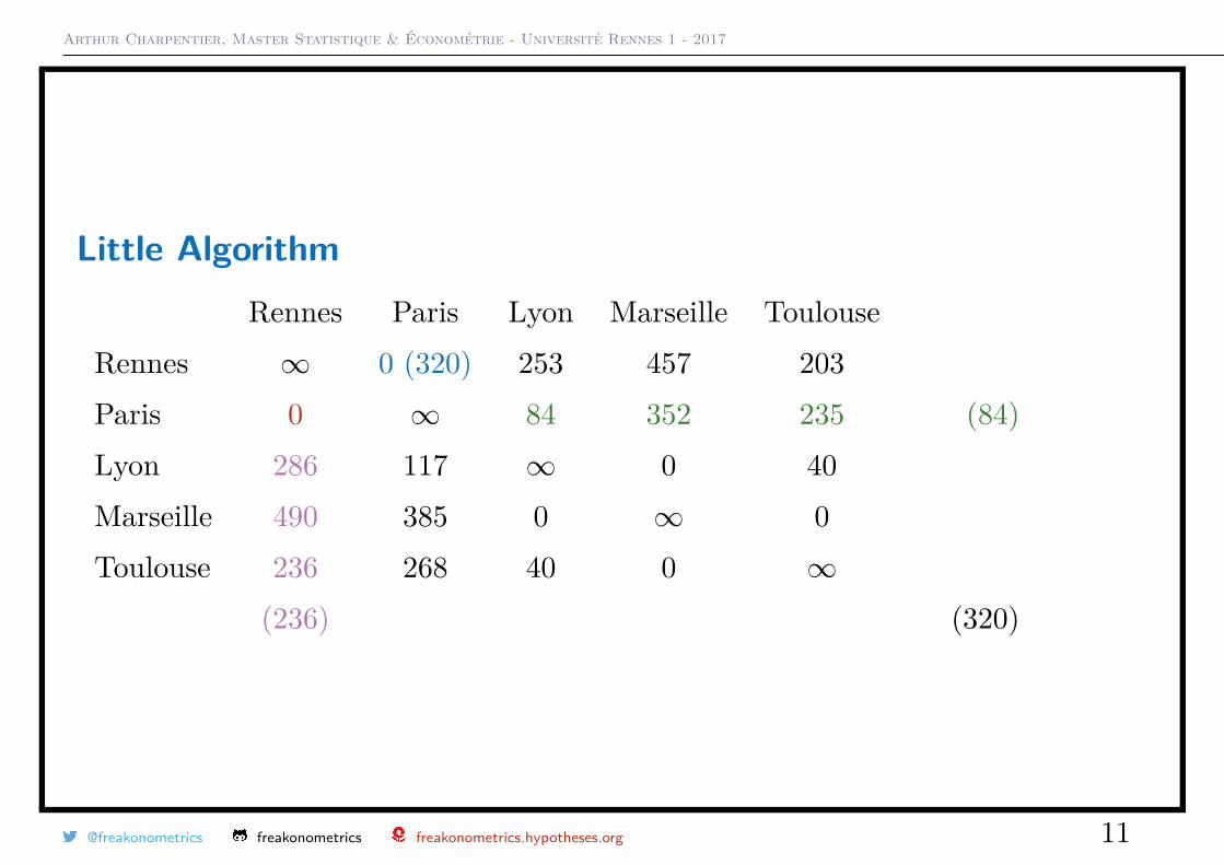
Little AlgorithmRennes Paris Lyon Marseille Toulouse
Rennes ∞ 0 (320) 253 457 203Paris 0 ∞ 84 352 235 (84)Lyon 286 117 ∞ 0 40Marseille 490 385 0 ∞ 0Toulouse 236 268 40 0 ∞
(236) (320)
@freakonometrics freakonometrics freakonometrics.hypotheses.org 11
Arthur Charpentier, Master Statistique & Économétrie - Université Rennes 1 - 2017
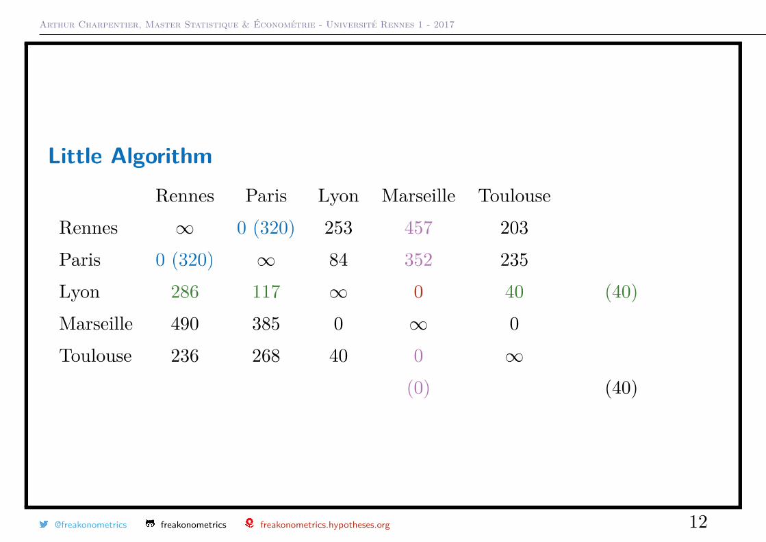
Little AlgorithmRennes Paris Lyon Marseille Toulouse
Rennes ∞ 0 (320) 253 457 203Paris 0 (320) ∞ 84 352 235Lyon 286 117 ∞ 0 40 (40)Marseille 490 385 0 ∞ 0Toulouse 236 268 40 0 ∞
(0) (40)
@freakonometrics freakonometrics freakonometrics.hypotheses.org 12
Arthur Charpentier, Master Statistique & Économétrie - Université Rennes 1 - 2017
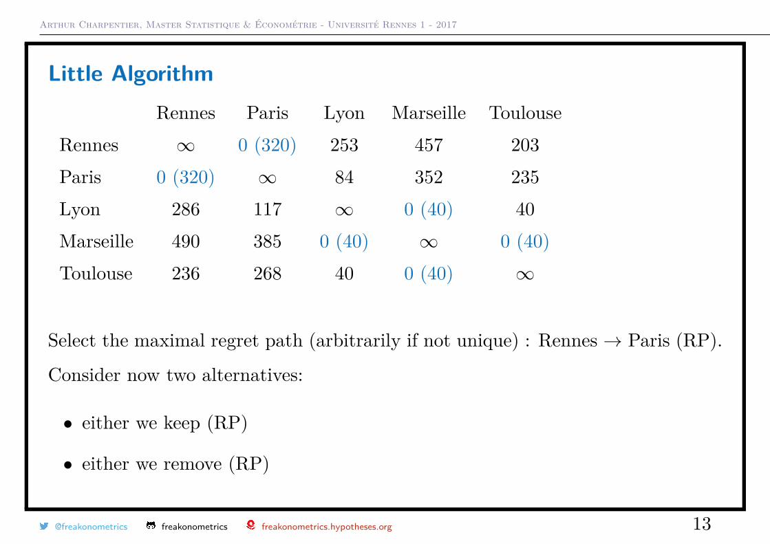
Little AlgorithmRennes Paris Lyon Marseille Toulouse
Rennes ∞ 0 (320) 253 457 203Paris 0 (320) ∞ 84 352 235Lyon 286 117 ∞ 0 (40) 40Marseille 490 385 0 (40) ∞ 0 (40)Toulouse 236 268 40 0 (40) ∞
Select the maximal regret path (arbitrarily if not unique) : Rennes → Paris (RP).
Consider now two alternatives:
• either we keep (RP)
• either we remove (RP)
@freakonometrics freakonometrics freakonometrics.hypotheses.org 13
Arthur Charpentier, Master Statistique & Économétrie - Université Rennes 1 - 2017
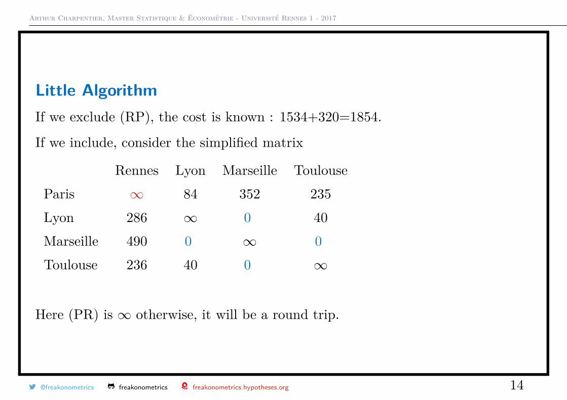
Little AlgorithmIf we exclude (RP), the cost is known : 1534+320=1854.
If we include, consider the simplified matrix
Rennes Lyon Marseille ToulouseParis ∞ 84 352 235Lyon 286 ∞ 0 40Marseille 490 0 ∞ 0Toulouse 236 40 0 ∞
Here (PR) is ∞ otherwise, it will be a round trip.
@freakonometrics freakonometrics freakonometrics.hypotheses.org 14
Arthur Charpentier, Master Statistique & Économétrie - Université Rennes 1 - 2017
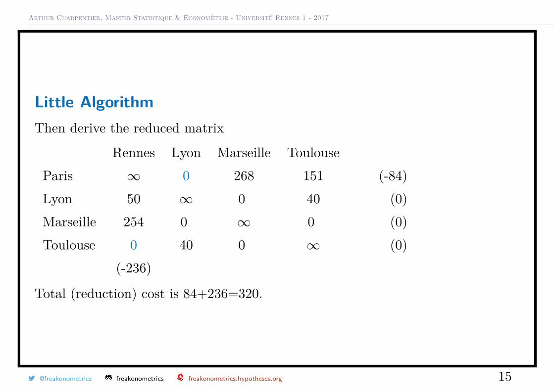
Little AlgorithmThen derive the reduced matrix
Rennes Lyon Marseille ToulouseParis ∞ 0 268 151 (-84)Lyon 50 ∞ 0 40 (0)Marseille 254 0 ∞ 0 (0)Toulouse 0 40 0 ∞ (0)
(-236)
Total (reduction) cost is 84+236=320.
@freakonometrics freakonometrics freakonometrics.hypotheses.org 15
Arthur Charpentier, Master Statistique & Économétrie - Université Rennes 1 - 2017
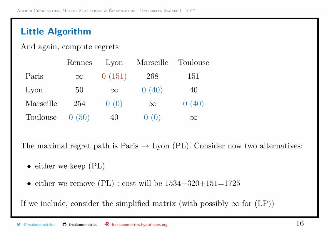
Little AlgorithmAnd again, compute regrets
Rennes Lyon Marseille ToulouseParis ∞ 0 (151) 268 151Lyon 50 ∞ 0 (40) 40Marseille 254 0 (0) ∞ 0 (40)Toulouse 0 (50) 40 0 (0) ∞
The maximal regret path is Paris → Lyon (PL). Consider now two alternatives:
• either we keep (PL)
• either we remove (PL) : cost will be 1534+320+151=1725
If we include, consider the simplified matrix (with possibly ∞ for (LP))
@freakonometrics freakonometrics freakonometrics.hypotheses.org 16
Arthur Charpentier, Master Statistique & Économétrie - Université Rennes 1 - 2017
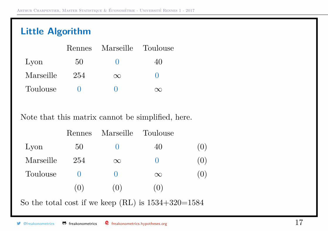
Little AlgorithmRennes Marseille Toulouse
Lyon 50 0 40Marseille 254 ∞ 0Toulouse 0 0 ∞
Note that this matrix cannot be simplified, here.
Rennes Marseille ToulouseLyon 50 0 40 (0)Marseille 254 ∞ 0 (0)Toulouse 0 0 ∞ (0)
(0) (0) (0)
So the total cost if we keep (RL) is 1534+320=1584
@freakonometrics freakonometrics freakonometrics.hypotheses.org 17
Arthur Charpentier, Master Statistique & Économétrie - Université Rennes 1 - 2017
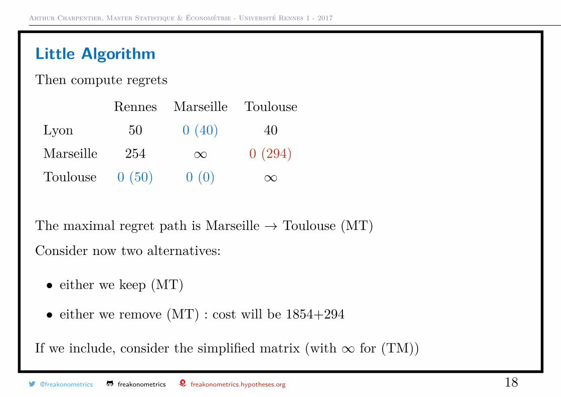
Little AlgorithmThen compute regrets
Rennes Marseille ToulouseLyon 50 0 (40) 40Marseille 254 ∞ 0 (294)Toulouse 0 (50) 0 (0) ∞
The maximal regret path is Marseille → Toulouse (MT)
Consider now two alternatives:
• either we keep (MT)
• either we remove (MT) : cost will be 1854+294
If we include, consider the simplified matrix (with ∞ for (TM))
@freakonometrics freakonometrics freakonometrics.hypotheses.org 18
Arthur Charpentier, Master Statistique & Économétrie - Université Rennes 1 - 2017
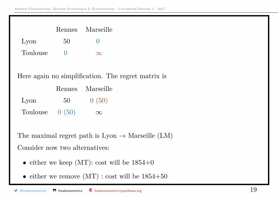
Rennes MarseilleLyon 50 0Toulouse 0 ∞
Here again no simplification. The regret matrix is
Rennes MarseilleLyon 50 0 (50)Toulouse 0 (50) ∞
The maximal regret path is Lyon → Marseille (LM)
Consider now two alternatives:
• either we keep (MT): cost will be 1854+0
• either we remove (MT) : cost will be 1854+50
@freakonometrics freakonometrics freakonometrics.hypotheses.org 19
Arthur Charpentier, Master Statistique & Économétrie - Université Rennes 1 - 2017
Little AlgorithmHere we have constructed a search tree.
click to visualize the construction click to visualize the construction
Remark This is an exact algorithm
@freakonometrics freakonometrics freakonometrics.hypotheses.org 20
Arthur Charpentier, Master Statistique & Économétrie - Université Rennes 1 - 2017
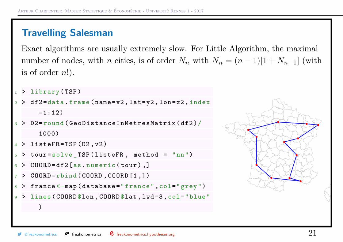
Travelling SalesmanExact algorithms are usually extremely slow. For Little Algorithm, the maximalnumber of nodes, with n cities, is of order Nn with Nn = (n− 1)[1 + Nn−1] (withis of order n!).
1 > library (TSP)
2 > df2=data. frame (name=v2 ,lat=y2 ,lon=x2 , index
=1:12)
3 > D2= round ( GeoDistanceInMetresMatrix (df2)/
1000)
4 > listeFR =TSP(D2 ,v2)
5 > tour= solve _TSP(listeFR , method = "nn")
6 > COORD =df2[as. numeric (tour) ,]
7 > COORD = rbind (COORD , COORD [1 ,])
8 > france <-map( database =" france ",col="grey")
9 > lines ( COORD $lon , COORD $lat ,lwd =3, col="blue"
)
@freakonometrics freakonometrics freakonometrics.hypotheses.org 21

Arthur Charpentier, Master Statistique & Économétrie - Université Rennes 1 - 2017
Travelling Salesman1 > tour= solve _TSP(listeFR , method = "nn")
2 > COORD =df2[as. numeric (tour) ,]
3 > COORD = rbind (COORD , COORD [1 ,])
4 > france <-map( database =" france ",col="grey")
5 > lines ( COORD $lon , COORD $lat ,lwd =3, col="blue")
6 >
7 > tour= solve _TSP(listeFR , method = "nn")
8 > COORD =df2[as. numeric (tour) ,]
9 > COORD = rbind (COORD , COORD [1 ,])
10 > france <-map( database =" france ",col="grey")
11 > lines ( COORD $lon , COORD $lat ,lwd =3, col="blue")
It is not stable... local optimization?
@freakonometrics freakonometrics freakonometrics.hypotheses.org 22
Arthur Charpentier, Master Statistique & Économétrie - Université Rennes 1 - 2017
Travelling Salesman
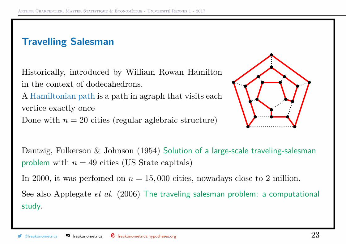
Historically, introduced by William Rowan Hamiltonin the context of dodecahedrons.A Hamiltonian path is a path in agraph that visits eachvertice exactly onceDone with n = 20 cities (regular aglebraic structure)
Dantzig, Fulkerson & Johnson (1954) Solution of a large-scale traveling-salesmanproblem with n = 49 cities (US State capitals)
In 2000, it was perfomed on n = 15, 000 cities, nowadays close to 2 million.
See also Applegate et al. (2006) The traveling salesman problem: a computationalstudy.
@freakonometrics freakonometrics freakonometrics.hypotheses.org 23
Arthur Charpentier, Master Statistique & Économétrie - Université Rennes 1 - 2017
Stochastic AlgorithmOne can use a Greedy AlgorithmHeuristically, makes locally optimal choices at each stagewith the hope of finding a global optimum.nearest neighbour, “at each stage visit an unvisited citynearest to the current city”(1) start on an arbitrary vertex as current vertice.(2) find out the shortest edge connecting current verticeand an unvisited vertice v.(3) set current vertice to v.(4) mark v as visited.(5) if all the vertices in domain are visited, then terminate.(6) Go to step 2.
click to visualize the construction
@freakonometrics freakonometrics freakonometrics.hypotheses.org 24
Arthur Charpentier, Master Statistique & Économétrie - Université Rennes 1 - 2017
Stochastic AlgorithmE.g. descent algorithm, where we start from an initial guess, then consider ateach step one vertice s, and in the neighborhood of s, denoted V (s) search
f(s?) = mins′∈V (s)
{f(s′)}
If f(s?) < f(s) then s = s?.
See Lin (1965) with 2 opt or 3 opt, see also Lin & Kernighan(1973) An Effective Heuristic Algorithm for the Traveling-Salesman ProblemThe pairwise exchange or 2-opt technique involves itera-tively removing two edges and replacing these with two dif-ferent edges that reconnect the fragments created by edgeremoval into a new and shorter tour.
click to visualize the construction
@freakonometrics freakonometrics freakonometrics.hypotheses.org 25
Arthur Charpentier, Master Statistique & Économétrie - Université Rennes 1 - 2017
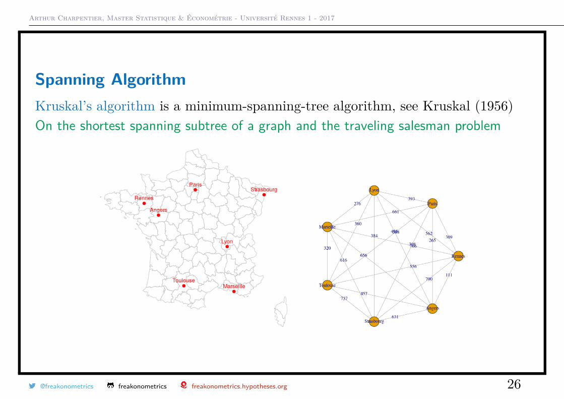
Spanning AlgorithmKruskal’s algorithm is a minimum-spanning-tree algorithm, see Kruskal (1956)On the shortest spanning subtree of a graph and the traveling salesman problem
@freakonometrics freakonometrics freakonometrics.hypotheses.org 26
Arthur Charpentier, Master Statistique & Économétrie - Université Rennes 1 - 2017
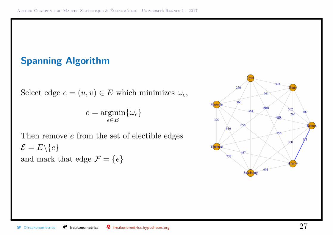
Spanning Algorithm
Select edge e = (u, v) ∈ E which minimizes ωε,
e = argminε∈E
{ωε}
Then remove e from the set of electible edgesE = E\{e}and mark that edge F = {e}
@freakonometrics freakonometrics freakonometrics.hypotheses.org 27
Arthur Charpentier, Master Statistique & Économétrie - Université Rennes 1 - 2017
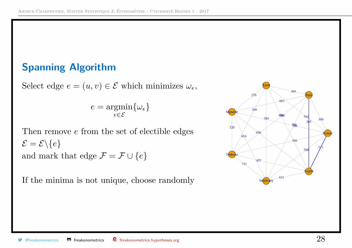
Spanning Algorithm
Select edge e = (u, v) ∈ E which minimizes ωε,
e = argminε∈E
{ωε}
Then remove e from the set of electible edgesE = E\{e}and mark that edge F = F ∪ {e}
If the minima is not unique, choose randomly
@freakonometrics freakonometrics freakonometrics.hypotheses.org 28
Arthur Charpentier, Master Statistique & Économétrie - Université Rennes 1 - 2017
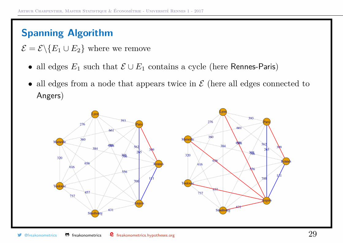
Spanning AlgorithmE = E\{E1 ∪ E2} where we remove
• all edges E1 such that E ∪ E1 contains a cycle (here Rennes-Paris)
• all edges from a node that appears twice in E (here all edges connected toAngers)
@freakonometrics freakonometrics freakonometrics.hypotheses.org 29
Arthur Charpentier, Master Statistique & Économétrie - Université Rennes 1 - 2017
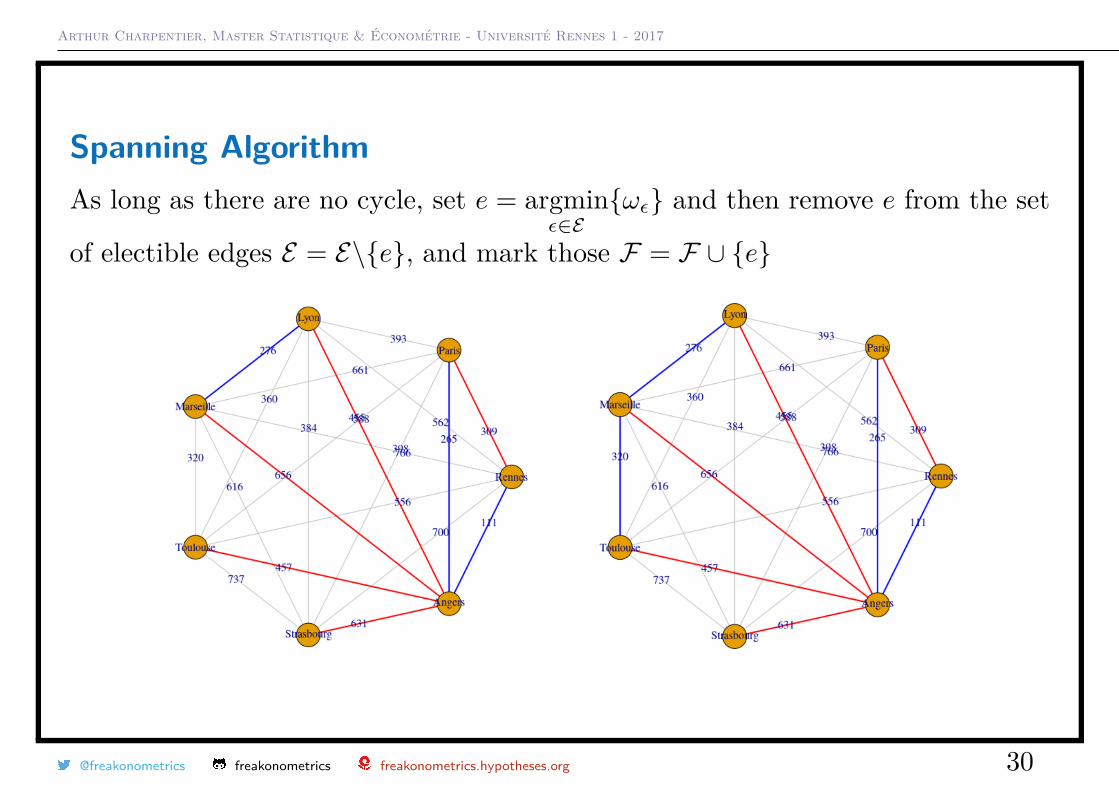
Spanning AlgorithmAs long as there are no cycle, set e = argmin
ε∈E{ωε} and then remove e from the set
of electible edges E = E\{e}, and mark those F = F ∪ {e}
@freakonometrics freakonometrics freakonometrics.hypotheses.org 30
Arthur Charpentier, Master Statistique & Économétrie - Université Rennes 1 - 2017
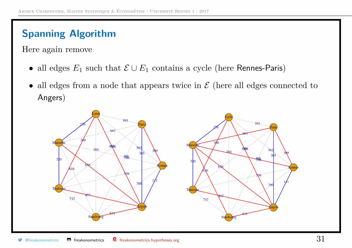
Spanning AlgorithmHere again remove
• all edges E1 such that E ∪ E1 contains a cycle (here Rennes-Paris)
• all edges from a node that appears twice in E (here all edges connected toAngers)
@freakonometrics freakonometrics freakonometrics.hypotheses.org 31
Arthur Charpentier, Master Statistique & Économétrie - Université Rennes 1 - 2017
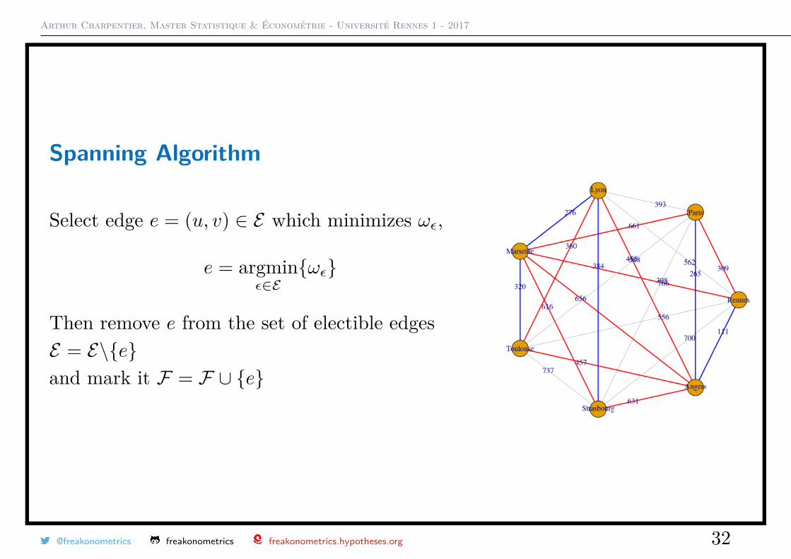
Spanning Algorithm
Select edge e = (u, v) ∈ E which minimizes ωε,
e = argminε∈E
{ωε}
Then remove e from the set of electible edgesE = E\{e}and mark it F = F ∪ {e}
@freakonometrics freakonometrics freakonometrics.hypotheses.org 32
Arthur Charpentier, Master Statistique & Économétrie - Université Rennes 1 - 2017
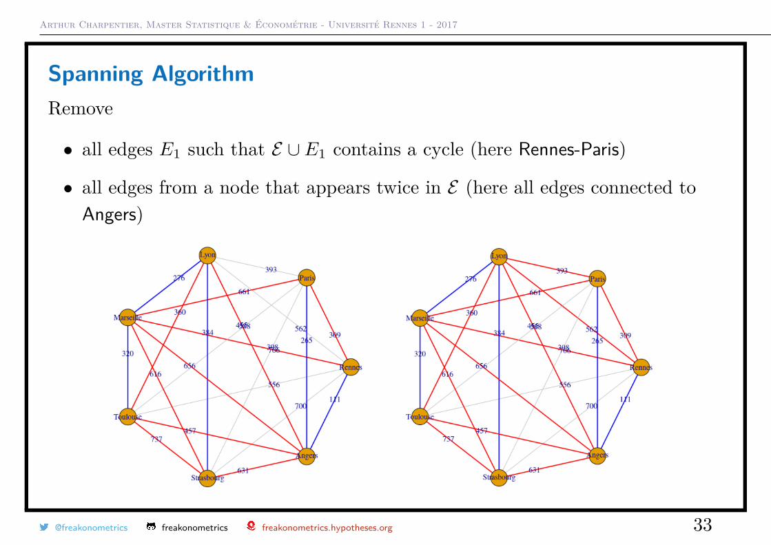
Spanning AlgorithmRemove
• all edges E1 such that E ∪ E1 contains a cycle (here Rennes-Paris)
• all edges from a node that appears twice in E (here all edges connected toAngers)
@freakonometrics freakonometrics freakonometrics.hypotheses.org 33
Arthur Charpentier, Master Statistique & Économétrie - Université Rennes 1 - 2017
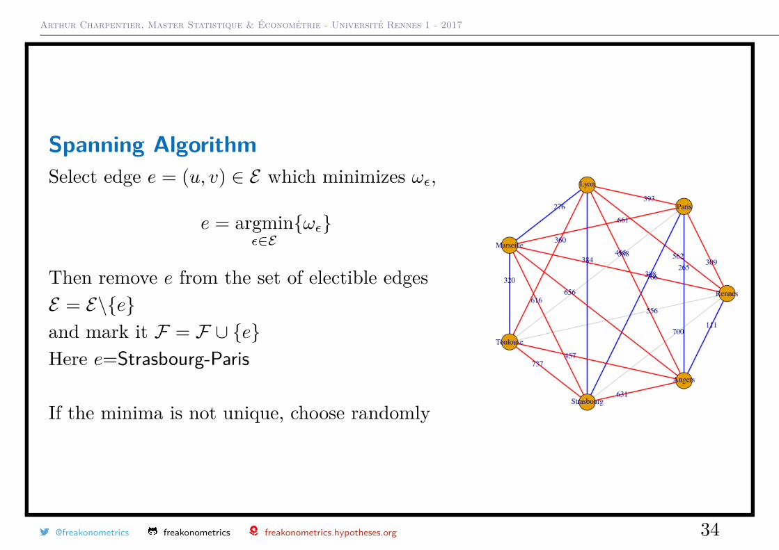
Spanning AlgorithmSelect edge e = (u, v) ∈ E which minimizes ωε,
e = argminε∈E
{ωε}
Then remove e from the set of electible edgesE = E\{e}and mark it F = F ∪ {e}Here e=Strasbourg-Paris
If the minima is not unique, choose randomly
@freakonometrics freakonometrics freakonometrics.hypotheses.org 34
Arthur Charpentier, Master Statistique & Économétrie - Université Rennes 1 - 2017
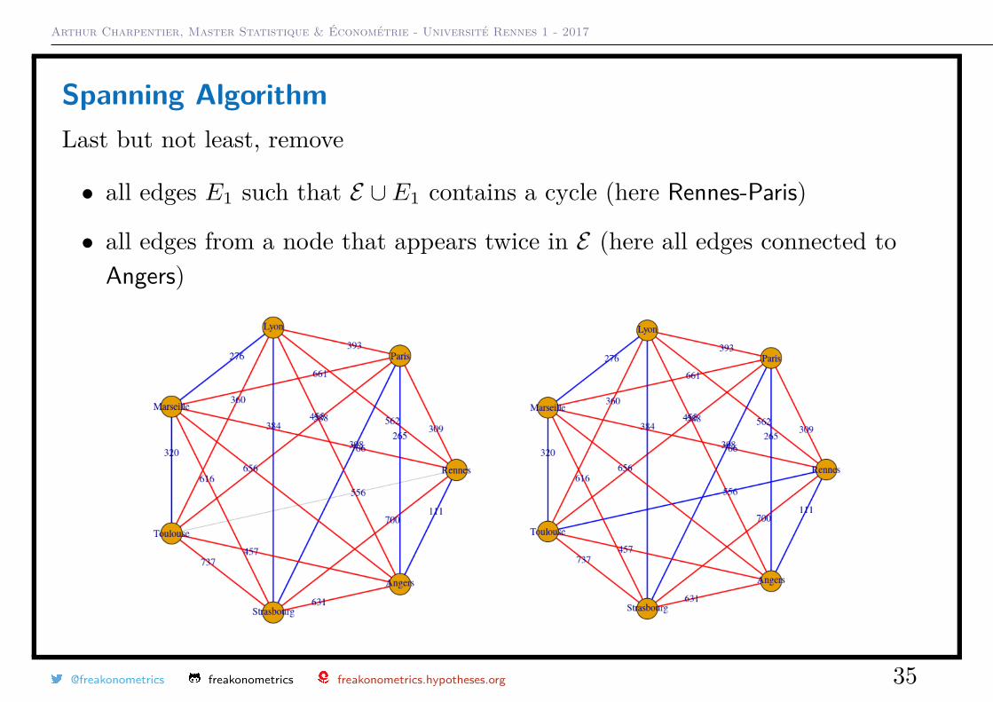
Spanning AlgorithmLast but not least, remove
• all edges E1 such that E ∪ E1 contains a cycle (here Rennes-Paris)
• all edges from a node that appears twice in E (here all edges connected toAngers)
@freakonometrics freakonometrics freakonometrics.hypotheses.org 35

Arthur Charpentier, Master Statistique & Économétrie - Université Rennes 1 - 2017
Spanning AlgorithmThe collection of edges that were marked in F is our best cycle.
@freakonometrics freakonometrics freakonometrics.hypotheses.org 36
Arthur Charpentier, Master Statistique & Économétrie - Université Rennes 1 - 2017
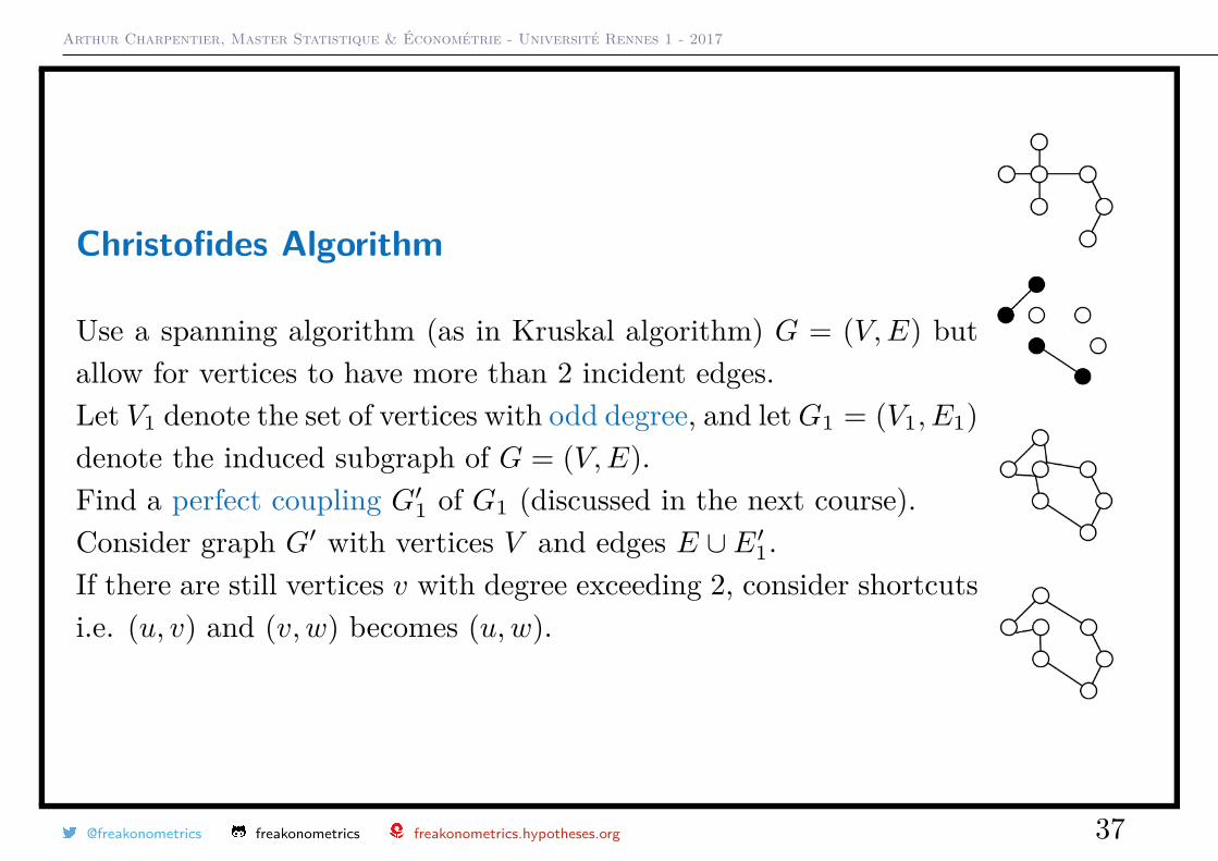
Christofides Algorithm
Use a spanning algorithm (as in Kruskal algorithm) G = (V, E) butallow for vertices to have more than 2 incident edges.Let V1 denote the set of vertices with odd degree, and let G1 = (V1, E1)denote the induced subgraph of G = (V, E).Find a perfect coupling G′1 of G1 (discussed in the next course).Consider graph G′ with vertices V and edges E ∪ E′1.If there are still vertices v with degree exceeding 2, consider shortcutsi.e. (u, v) and (v, w) becomes (u, w).
@freakonometrics freakonometrics freakonometrics.hypotheses.org 37
Arthur Charpentier, Master Statistique & Économétrie - Université Rennes 1 - 2017
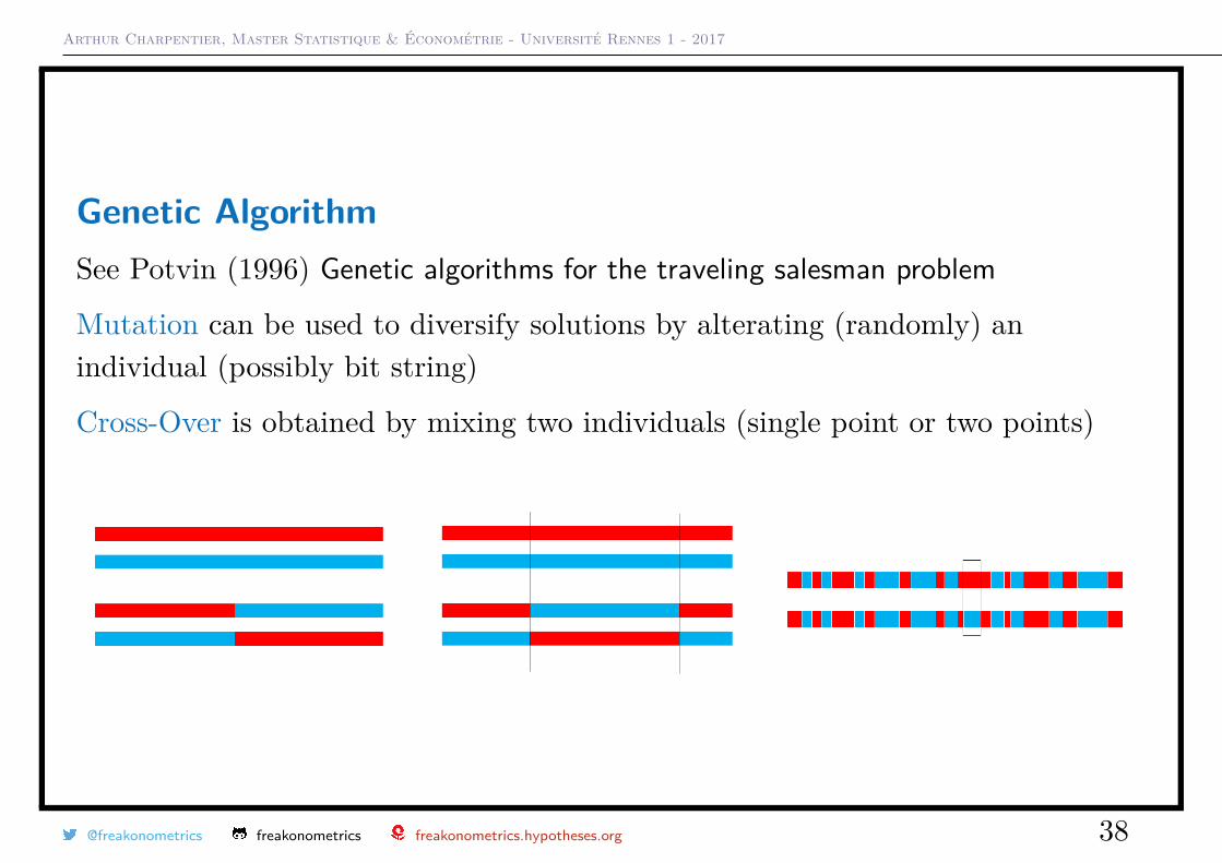
Genetic AlgorithmSee Potvin (1996) Genetic algorithms for the traveling salesman problem
Mutation can be used to diversify solutions by alterating (randomly) anindividual (possibly bit string)
Cross-Over is obtained by mixing two individuals (single point or two points)
@freakonometrics freakonometrics freakonometrics.hypotheses.org 38

Arthur Charpentier, Master Statistique & Économétrie - Université Rennes 1 - 2017
Travelling SalesmanCan be performed on a (much) larger scalee.g. 48 State capitals in mainland U.S.
see Cook (2011) In Pursuit of the Traveling Salesmanfor a survey.
@freakonometrics freakonometrics freakonometrics.hypotheses.org 39