![Constrained Convolutional Neural Networks for …vgg/rg/slides/ccnn1.pdf · Constrained Convolutional Neural Networks for Weakly Supervised Segmentation ... [CCNN] Convolutional Neural](https://static.fdocuments.us/doc/165x107/5baa6a3809d3f2c9618bd4b3/constrained-convolutional-neural-networks-for-vggrgslidesccnn1pdf-constrained.jpg)
Neural Networks slides
19
Artificial Intelligence: Representation and Problem Solving 15-381 January 16, 2007 Neural Networks Michael S. Lewicki ! Carnegie Mellon Artificial Intelligence: Neural Networks Topics • decision boundaries • linear discriminants • perceptron • gradient learning • neural networks 2
Transcript of Neural Networks slides

Artificial Intelligence: Representation and Problem
Solving
15-381
January 16, 2007
Neural Networks
Michael S. Lewicki ! Carnegie MellonArtificial Intelligence: Neural Networks
Topics
• decision boundaries
• linear discriminants
• perceptron
• gradient learning
• neural networks
2

Michael S. Lewicki ! Carnegie MellonArtificial Intelligence: Neural Networks
The Iris dataset with decision tree boundaries
3
1 2 3 4 5 6 70
0.5
1
1.5
2
2.5
petal length (cm)
peta
l w
idth
(cm
)
Michael S. Lewicki ! Carnegie MellonArtificial Intelligence: Neural Networks
The optimal decision boundary for C2 vs C3
4
1 2 3 4 5 6 70
0.5
1
1.5
2
2.5
petal length (cm)
pe
tal w
idth
(cm
)
0
0.1
0.2
0.3
0.4
0.5
0.6
0.7
0.8
0.9p(petal length |C2) p(petal length |C3) • optimal decision boundary is
determined from the statistical distribution of the classes
• optimal only if model is correct!
• assigns precise degree of uncertainty to classification

Michael S. Lewicki ! Carnegie MellonArtificial Intelligence: Neural Networks
Optimal decision boundary
5
1 2 3 4 5 6 70
0.2
0.4
0.6
0.8
1
Optimal decision boundary
p(petal length |C2) p(petal length |C3)
p(C2 | petal length) p(C3 | petal length)
Michael S. Lewicki ! Carnegie MellonArtificial Intelligence: Neural Networks
Can we do better?
6
1 2 3 4 5 6 70
0.5
1
1.5
2
2.5
petal length (cm)
pe
tal w
idth
(cm
)
0
0.1
0.2
0.3
0.4
0.5
0.6
0.7
0.8
0.9p(petal length |C2) p(petal length |C3) • only way is to use more information
• DTs use both petal width and petal length

Michael S. Lewicki ! Carnegie MellonArtificial Intelligence: Neural Networks
Arbitrary decision boundaries would be more powerful
7
1 2 3 4 5 6 70
0.5
1
1.5
2
2.5
petal length (cm)
peta
l w
idth
(cm
)
Decision boundaries could be non-linear
Michael S. Lewicki ! Carnegie MellonArtificial Intelligence: Neural Networks
3 4 5 6 7
1
1.5
2
2.5
x1
x2
Defining a decision boundary
8
• consider just two classes
• want points on one side of line in class 1, otherwise class 2.
• 2D linear discriminant function:
• This defines a 2D plane which leads to the decision:
The decision boundary:
y = mT x + b = 0x ∈
{class 1 if y ≥ 0,class 2 if y < 0.
m1x1 + m2x2 = −b
⇒ x2 = −m1x1 + b
m2
Or in terms of scalars:
y = mT x + b
= m1x1 + m2x2 + b
=∑
i
mixi + b

Michael S. Lewicki ! Carnegie MellonArtificial Intelligence: Neural Networks
Linear separability
9
1 2 3 4 5 6 70
0.5
1
1.5
2
2.5
petal length (cm)
peta
l w
idth
(cm
)
• Two classes are linearly separable if they can be separated by a linear combination of attributes
- 1D: threshold
- 2D: line
- 3D: plane
- M-D: hyperplane
linearly separable
not linearly separable
Michael S. Lewicki ! Carnegie MellonArtificial Intelligence: Neural Networks
Diagraming the classifier as a “neural” network
• The feedforward neural network is specified by weights wi and bias b:
• It can written equivalently as
• where w0 = b is the bias and a
“dummy” input x0 that is always 1.
10
x1 x2 xM• •!•
y
w1 w2 wM
b
x1 x2 xM• •!•
y
w1 w2 wM
x0=1
w0
y = wT x =M∑
i=0
wixi
y = wT x + b
=M∑
i=1
wixi + b
“output unit”
“input units”
“bias”
“weights”

Michael S. Lewicki ! Carnegie MellonArtificial Intelligence: Neural Networks
Determining, ie learning, the optimal linear discriminant
11
• First we must define an objective function, ie the goal of learning
• Simple idea: adjust weights so that output y(xn) matches class cn
• Objective: minimize sum-squared error over all patterns xn:
• Note the notation xn defines a pattern vector:
• We can define the desired class as:
E =12
N∑
n=1
(wT xn − cn)2
xn = {x1, . . . , xM}n
cn =
{0 xn ∈ class 11 xn ∈ class 2
Michael S. Lewicki ! Carnegie MellonArtificial Intelligence: Neural Networks
We’ve seen this before: curve fitting
12
example from Bishop (2006), Pattern Recognition and Machine Learning
t = sin(2πx) + noise
0 1
!1
0
1t
x
y(xn,w)
tn
xn

Michael S. Lewicki ! Carnegie MellonArtificial Intelligence: Neural Networks
Neural networks compared to polynomial curve fitting
13
0 1
!1
0
1
0 1
!1
0
1
0 1
!1
0
1
0 1
!1
0
1
y(x,w) = w0 + w1x + w2x2 + · · · + wMxM =
M∑
j=0
wjxj
E(w) =12
N∑
n=1
[y(xn,w)− tn]2
example from Bishop (2006), Pattern Recognition and Machine Learning
For the linear network, M=1 and there are multiple input dimensions
Michael S. Lewicki ! Carnegie MellonArtificial Intelligence: Neural Networks
General form of a linear network
• A linear neural network is simply a linear transformation of the input.
• Or, in matrix-vector form:
• Multiple outputs corresponds to multivariate regression
14
y = Wx
yj =
M∑
i=0
wi,jxi
x1 xi xM• •!•
yi
wij
x0=1
y1 yK
• •!•
• •!•• •!•
x
y
W
“outputs”
“weights”
“inputs”
“bias”

Michael S. Lewicki ! Carnegie MellonArtificial Intelligence: Neural Networks
Training the network: Optimization by gradient descent
15
• We can adjust the weights incrementally to minimize the objective function.
• This is called gradient descent
• Or gradient ascent if we’re maximizing.
• The gradient descent rule for weight wi is:
• Or in vector form:
• For gradient ascent, the sign
of the gradient step changes.
w1
w2
w3
w4w2
w1
wt+1i
= wt
i − ε∂E
wi
wt+1 = wt − ε∂E
w
Michael S. Lewicki ! Carnegie MellonArtificial Intelligence: Neural Networks
Computing the gradient
• Idea: minimize error by gradient descent
• Take the derivative of the objective function wrt the weights:
• And in vector form:
16
E =12
N∑
n=1
(wT xn − cn)2
∂E
wi=
22
N∑
n=1
(w0x0,n + · · · + wixi,n + · · · + wMxM,n − cn)xi,n
=N∑
n=1
(wT xn − cn)xi,n
∂E
w=
N∑
n=1
(wT xn − cn)xn

Michael S. Lewicki ! Carnegie MellonArtificial Intelligence: Neural Networks
Simulation: learning the decision boundary
• Each iteration updates the gradient:
• Epsilon is a small value:
" = 0.1/N
• Epsilon too large:
- learning diverges
• Epsilon too small:
- convergence slow
17
3 4 5 6 7
1
1.5
2
2.5
x1
x2
0 5 10 151000
2000
3000
4000
5000
6000
7000
8000
9000
10000
11000
iteration
Error
∂E
wi
=N∑
n=1
(wTxn − cn)xi,n
wt+1i
= wt
i − ε∂E
wi
Learning Curve
Michael S. Lewicki ! Carnegie MellonArtificial Intelligence: Neural Networks
Simulation: learning the decision boundary
• Each iteration updates the gradient:
• Epsilon is a small value:
" = 0.1/N
• Epsilon too large:
- learning diverges
• Epsilon too small:
- convergence slow
18
3 4 5 6 7
1
1.5
2
2.5
x1
x2
0 5 10 151000
2000
3000
4000
5000
6000
7000
8000
9000
10000
11000
iteration
Error
∂E
wi
=N∑
n=1
(wTxn − cn)xi,n
wt+1i
= wt
i − ε∂E
wi
Learning Curve
Michael S. Lewicki ! Carnegie MellonArtificial Intelligence: Neural Networks
Simulation: learning the decision boundary
• Each iteration updates the gradient:
• Epsilon is a small value:
" = 0.1/N
• Epsilon too large:
- learning diverges
• Epsilon too small:
- convergence slow
19
3 4 5 6 7
1
1.5
2
2.5
x1
x2
0 5 10 151000
2000
3000
4000
5000
6000
7000
8000
9000
10000
11000
iteration
Error
∂E
wi
=N∑
n=1
(wTxn − cn)xi,n
wt+1i
= wt
i − ε∂E
wi
Learning Curve
Michael S. Lewicki ! Carnegie MellonArtificial Intelligence: Neural Networks
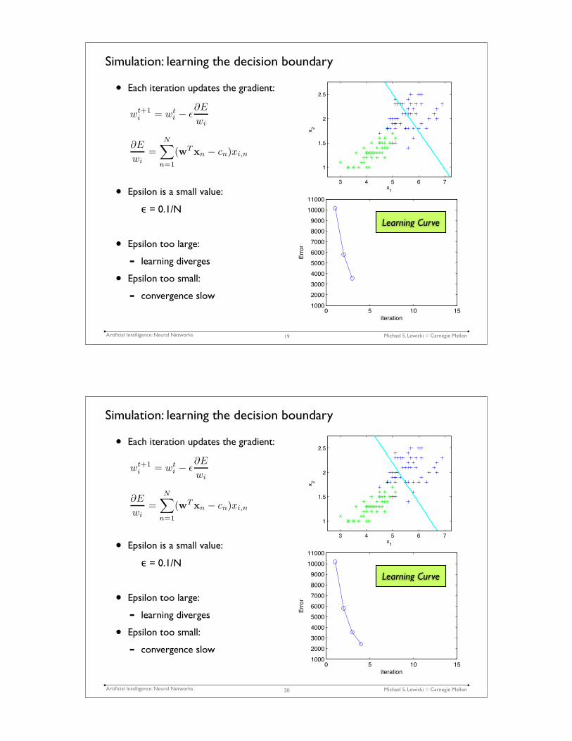
Simulation: learning the decision boundary
• Each iteration updates the gradient:
• Epsilon is a small value:
" = 0.1/N
• Epsilon too large:
- learning diverges
• Epsilon too small:
- convergence slow
20
3 4 5 6 7
1
1.5
2
2.5
x1
x2
0 5 10 151000
2000
3000
4000
5000
6000
7000
8000
9000
10000
11000
iteration
Error
∂E
wi
=N∑
n=1
(wTxn − cn)xi,n
wt+1i
= wt
i − ε∂E
wi
Learning Curve

Michael S. Lewicki ! Carnegie MellonArtificial Intelligence: Neural Networks
Simulation: learning the decision boundary
• Each iteration updates the gradient:
• Epsilon is a small value:
" = 0.1/N
• Epsilon too large:
- learning diverges
• Epsilon too small:
- convergence slow
21
3 4 5 6 7
1
1.5
2
2.5
x1
x2
0 5 10 151000
2000
3000
4000
5000
6000
7000
8000
9000
10000
11000
iteration
Error
∂E
wi
=N∑
n=1
(wTxn − cn)xi,n
wt+1i
= wt
i − ε∂E
wi
Learning Curve
Michael S. Lewicki ! Carnegie MellonArtificial Intelligence: Neural Networks
Simulation: learning the decision boundary
• Each iteration updates the gradient:
• Epsilon is a small value:
" = 0.1/N
• Epsilon too large:
- learning diverges
• Epsilon too small:
- convergence slow
22
3 4 5 6 7
1
1.5
2
2.5
x1
x2
0 5 10 151000
2000
3000
4000
5000
6000
7000
8000
9000
10000
11000
iteration
Error
∂E
wi
=N∑
n=1
(wTxn − cn)xi,n
wt+1i
= wt
i − ε∂E
wi
Learning Curve

Michael S. Lewicki ! Carnegie MellonArtificial Intelligence: Neural Networks
Simulation: learning the decision boundary
• Learning converges onto the solution that minimizes the error.
• For linear networks, this is guaranteed to converge to the minimum
• It is also possible to derive a closed-form solution (covered later)
23
3 4 5 6 7
1
1.5
2
2.5
x1
x2
0 5 10 151000
2000
3000
4000
5000
6000
7000
8000
9000
10000
11000
iteration
Error
Learning Curve
Michael S. Lewicki ! Carnegie MellonArtificial Intelligence: Neural Networks
Learning is slow when epsilon is too small
• Here, larger step sizes would converge more quickly to the minimum
24
w
Error

Michael S. Lewicki ! Carnegie MellonArtificial Intelligence: Neural Networks
Divergence when epsilon is too large
• If the step size is too large, learning can oscillate between different sides of the minimum
25
w
Error
Michael S. Lewicki ! Carnegie MellonArtificial Intelligence: Neural Networks
Multi-layer networks
26
• Can we extend our network to multiple layers? We have:
• Or in matrix form
• Thus a two-layer linear network is equivalent to a one-layer linear network with weights U=VW.
• It is not more powerful.
x
y
W
V
z
yj =
∑
i
wi,jxi
zj =
∑
k
vj,kyj
=
∑
k
vj,k
∑
i
wi,jxi
z = Vy
= VWx
How do we address this?

Michael S. Lewicki ! Carnegie MellonArtificial Intelligence: Neural Networks
Non-linear neural networks
• Idea introduce a non-linearity:
• Now, multiple layers are not equivalent
• Common nonlinearities:
- threshold
- sigmoid
27
yj = f(∑
i
wi,jxi)
zj = f(∑
k
vj,k yj)
= f(∑
k
vj,k f(∑
i
wi,jxi))
!! !" !# !$ !% & % $ # " !&
%
'
()'*
threshold
!! !" !# !$ !% & % $ # " !&
%
'()'*
sigmoid
y =
{
0 x < 0
1 x ≥ 0
y =1
1 + exp(−x)
Michael S. Lewicki ! Carnegie MellonArtificial Intelligence: Neural Networks
Modeling logical operators
• A one-layer binary-threshold network can implement the logical operators AND and OR, but not XOR.
• Why not?
28
x1
x2
x1
x2
x1
x2
x1 AND x2 x1 OR x2 x1 XOR x2
yj = f(∑
i
wi,jxi)
!! !" !# !$ !% & % $ # " !&
%
'
()'*
threshold y =
{
0 x < 0
1 x ≥ 0

Michael S. Lewicki ! Carnegie MellonArtificial Intelligence: Neural Networks
Posterior odds interpretation of a sigmoid
29
Michael S. Lewicki ! Carnegie MellonArtificial Intelligence: Neural Networks
The general classification/regression problem
30
Data
D = {x1, . . . ,xT }
xi = {x1, . . . , xN}i
desired output
y = {y1, . . . , yK}
model
θ = {θ1, . . . , θM}
Given data, we want to learn a model that can correctly classify novel observations or
map the inputs to the outputs
yi =
{1 if xi ∈ Ci ≡ class i,
0 otherwise
for classification:
input is a set of T observations, each an N-dimensional vector (binary, discrete, or continuous)
model (e.g. a decision tree) is defined by M parameters, e.g. a multi-layer neural network.
regression for arbitrary y.

Michael S. Lewicki ! Carnegie MellonArtificial Intelligence: Neural Networks
• Error function is defined as before, where we use the target vector tn to define the desired output for network output yn.
• The “forward pass” computes the outputs at each layer:
A general multi-layer neural network
31
E =1
2
N∑
n=1
(yn(xn,W1:L) − tn)2
x1 xi xM• •!•
yi
wij
x0=1
y1 yK
• •!•
• •!•• •!•
x0=1
yiy1 yK• •!•• •!•
yiy1 yK• •!•• •!•
y0=1
wij
• •!•
y0=1
ylj = f(
∑
i
wli,j yl−1
j )
l = {1, . . . , L}
x ≡ y0
output = yL
input
layer 1
layer 2
output
Michael S. Lewicki ! Carnegie MellonArtificial Intelligence: Neural Networks
Deriving the gradient for a sigmoid neural network
• Mathematical procedure for train is gradient descient: same as before, except the gradients are more complex to derive.
• Convenient fact for the sigmoid non-linearity:
• backward pass computes the gradients: back-propagation
32
dσ(x)
dx=
d
dx
1
1 + exp (−x)
= σ(x)(1 − σ(x))
E =1
2
N∑
n=1
(yn(xn,W1:L) − tn)2
x1 xi xM• •!•
yi
wij
x0=1
y1 yK
• •!•
• •!•• •!•
x0=1
yiy1 yK• •!•• •!•
yiy1 yK• •!•• •!•
y0=1
wij
• •!•
y0=1
input
layer 1
layer 2
output
Wt+1 = Wt + ε∂E
W
New problem: local minima

Michael S. Lewicki ! Carnegie MellonArtificial Intelligence: Neural Networks
Applications: Driving (output is analog: steering direction)
33
24
Real Examplenetwork with 1 layer
(4 hidden units)
D. Pomerleau. Neural network perception for mobile robot guidance. Kluwer Academic Publishing, 1993.
• Learns to drive on roads• Demonstrated at highway speeds over 100s of miles
Training data: Images +
corresponding steering angle
Important: Conditioning of training data to generate new examples ! avoids overfitting
Michael S. Lewicki ! Carnegie MellonArtificial Intelligence: Neural Networks
Real image input is augmented to avoid overfitting
34
24
Real Examplenetwork with 1 layer
(4 hidden units)
D. Pomerleau. Neural network perception for mobile robot guidance. Kluwer Academic Publishing, 1993.
• Learns to drive on roads• Demonstrated at highway speeds over 100s of miles
Training data: Images +
corresponding steering angle
Important: Conditioning of training data to generate new examples ! avoids overfitting

Michael S. Lewicki ! Carnegie MellonArtificial Intelligence: Neural Networks
23
Real Example
• Takes as input image of handwritten digit• Each pixel is an input unit• Complex network with many layers• Output is digit class
• Tested on large (50,000+) database of handwritten samples• Real-time• Used commercially
Y. LeCun, L. Bottou, Y. Bengio, and P. Haffner. Gradient-based learning applied to document recognition. Proceedings of the IEEE, november1998.
http://yann.lecun.com/exdb/lenet/
Very low error rate (<< 1%
Hand-written digits: LeNet
35
Michael S. Lewicki ! Carnegie MellonArtificial Intelligence: Neural Networks
LeNet
36
23
Real Example
• Takes as input image of handwritten digit• Each pixel is an input unit• Complex network with many layers• Output is digit class
• Tested on large (50,000+) database of handwritten samples• Real-time• Used commercially
Y. LeCun, L. Bottou, Y. Bengio, and P. Haffner. Gradient-based learning applied to document recognition. Proceedings of the IEEE, november1998.
http://yann.lecun.com/exdb/lenet/
Very low error rate (<< 1%
http://yann.lecun.com/exdb/lenet/

Michael S. Lewicki ! Carnegie MellonArtificial Intelligence: Neural Networks
Object recognition
• LeCun, Huang, Bottou (2004). Learning Methods for Generic Object Recognition with Invariance to Pose and Lighting. Proceedings of CVPR 2004.
• http://www.cs.nyu.edu/~yann/research/norb/
37
Michael S. Lewicki ! Carnegie MellonArtificial Intelligence: Neural Networks
Summary
• Decision boundaries
- Bayes optimal
- linear discriminant
- linear separability
• Classification vs regression
• Optimization by gradient descent
• Degeneracy of a multi-layer linear network
• Non-linearities:: threshold, sigmoid, others?
• Issues:
- very general architecture, can solve many problems
- large number of parameters: need to avoid overfitting
- usually requires a large amount of data, or special architecture
- local minima, training can be slow, need to set stepsize
38