SCREENING OF THE BACTERIAL REDUCTIVE

DECHLORINATION POTENTIAL OF

CHLORINATED ETHENES IN CONTAMINATED

AQUIFERS  

 

 

 

 

A TECHNICAL ASSISTANCE MANUAL FOR ASSESSMENT OF NATURAL 

ATTENUATION OF CHLOROETHENES‐CONTAMINATED SITES  

 

 

 

 

 

 

 

 

 

 

 

 

  Laboratoire de Biotechnologie Environnementale 

  Dr. Sonia‐Estelle Tarnawski 

  Dr. Pierre Rossi 

  Prof. Christof Holliger  

 

 

 

 

 

 

March 1st, 2016; final version   

   

 

 

 

 

 

 

 

 

 

 

 

 

 

 

 

 

 

 

 

 

 

 

 

 

 

 

 

 

 

 

 

 

 

 

 

 

 

 

 

 

 

Document prepared for the Swiss Federal Office for Environment –FOEN (OFEV)  

Mandates N°:  UTF 433.29.12 / IDM 2006.2423.389 and 00.0143.PZ / M133‐1537 

 

 

   

 

TABLE OF CONTENTS  List of acronyms ......................................................................................................................................... 1 Glossary ..................................................................................................................................................... 2 1. Introduction ............................................................................................................................................ 5

1.1. General context ..................................................................................................................... 5 1.2. The chlorinated ethenes........................................................................................................ 5 1.3. Conceptual framework of this manual and methodological principles ................................. 6 1.4. Keys for using the manual .................................................................................................... 7 1.5. Target audience .................................................................................................................... 7

2. Objectives .............................................................................................................................................. 8 "How does it work?” ...................................................................................................................... 8

3. Steps of the diagnostic tool ................................................................................................................... 9 4. Assessing in situ presence of reductive dechlorination ...................................................................... 11

4.1. Basis for the screening ........................................................................................................ 11 4.2. Water sampling strategy or monitoring well network .......................................................... 12 4.3. Parameters to evaluate for appreciation of in situ state of reductive dechlorination ......... 13 4.3.1. Contaminant map ............................................................................................................. 13 4.3.2. Interpretation of contaminant concentrations and detected end products ...................... 14 4.4. Parameters for evaluation of GWS physicochemistry and redox conditions ..................... 15 4.4.1. Predominant terminal electron-accepting processes ...................................................... 15 4.4.2. Parameters to evaluate the redox conditions of the GWS .............................................. 16 4.4.2.1. General parameters and descriptions .......................................................................... 17 4.3.2.2. Chemical parameters .................................................................................................... 17

5. Potential for reductive dechlorination of CEs ...................................................................................... 20 5.1. Looking for biomarkers in aquifer samples: Organohalide-respiring bacteria and reductive dehalogenase genes detection .................................................................................................. 21 5.1.1. Biodegradation processes of chlorinated-ethenes (Bradley, 2003) ................................ 21 5.1.2. Biomarkers of the reductive dechlorination process ....................................................... 22 5.2. Evaluation for potential of reductive dechlorination by specific detection of the presence of known OHRB and reductive dehalogenase genes .................................................................... 23 5.2.1. Water sampling: collection, transportation and storage. ................................................. 23 5.2.2. Sample filtration and DNA extraction ............................................................................... 24 5.2.3. PCR specific detections of OHRB and RdhA genes ....................................................... 24 5.3. Evaluation of the intrinsic reductive dechlorination potential of the GWS using microcosm experiments ................................................................................................................................ 24 5.4. Basis for interpretation of the microbial analyses ............................................................... 25

6. Aquifer biogeochemistry ...................................................................................................................... 27 6.1. Assessment of the bacterial community structures of the groundwater system ................ 28 6.2. Preparation of data for statistical analysis .......................................................................... 28 6.2.1. T-RFLP profiles ................................................................................................................ 29 6.2.2. Physicochemical data ...................................................................................................... 30 6.3. Multivariate statistical analysis for integrative analysis of bacterial and environmental data .................................................................................................................................................... 32 6.3.1. Procedure for the statistical analysis ............................................................................... 33 6.4. Keys for reading MFA plots ................................................................................................. 34 6.5. Guidelines for MFA interpretation and setting up the GWS biogeochemical model .......... 36

7. Case studies ........................................................................................................................................ 38 Application of the screening procedure for the evaluation of the natural attenuation potential in CEs-

contaminated aquifers .................................................................................................................. 38

7.1. Case study 1 - Former dry-cleaning facility, Canton of Solothurn, Switzerland ................. 38 7.2. Case study 2 - Former municipal discharge site, Canton of Geneva, Switzerland ........... 39 7.2.1. Site information ................................................................................................................ 39

7.2.2. Assessing in situ presence of reductive dechlorination – Step 1 .................................... 40 7.2.3. Evaluation of the biochemical potential for reductive dechlorination - Step 2 ................ 42 7.2.3.1. Detection of biomarkers ................................................................................................ 42 7.2.3.2. Microcosm experiments ................................................................................................ 43 7.2.4. Biogeochemistry of the aquifer: elucidate the reason for the observed incomplete reductive dechlorination of PCE – Step 3 .................................................................................. 45 7.2.4.1. Bacterial community structure investigation ................................................................. 45 7.2.4.2. Statistical analysis of the entire data set ...................................................................... 45 Output files of the statistical analysis ........................................... Error! Bookmark not defined. 7.2.4.3. Interpretations of the statistical analysis output plots ................................................... 47 7.2.4.4. Analysis of relations between environmental variables and BCS ................................ 49 7.2.5. Conclusions - Scenarios for incomplete in situ reductive dechlorination ........................ 51

References ............................................................................................................................................... 52 Appendix 1 ............................................................................................................................................... 56

Groundwater quality ........................................................................................................................ 56

Appendix 2 ............................................................................................................................................... 58 Chlorinated ethenes analyses ........................................................................................................ 58

Appendix 3 ............................................................................................................................................... 59 DNA extraction protocol .................................................................................................................. 59

Appendix 4 ............................................................................................................................................... 61 PCR protocol ................................................................................................................................... 61

Appendix 5 ............................................................................................................................................... 64 Enrichment culture .......................................................................................................................... 64

Appendix 6 ............................................................................................................................................... 68 T-RFLP procedure .......................................................................................................................... 68

Appendix 7 ............................................................................................................................................... 69 Installation of R software ................................................................................................................ 69

Appendix 8 ............................................................................................................................................... 70 Detail of ‘evplot.R’ function ............................................................................................................. 70

Appendix 9 ............................................................................................................................................... 71 Detail of the MFA script .................................................................................................................. 71

Appendix 10A ........................................................................................................................................... 77 Case study – Physicochemical data ............................................................................................... 77

Appendix 10B ........................................................................................................................................... 78 Case study – Bacterial community structure data .......................................................................... 78

 

 

DIAGRAMS, TABLES AND FIGURES  

 

Diagram 1 - Systematic treatment of contaminated site in 4 phases (modified from FOEN, 2001a) ..... 8 Diagram 2 – Systematic screening process, in three steps, for the evaluation of the potential of reductive dechlorination in an aquifer contaminated with chlorinated ethenes. ..................................................... 10 Diagram 3 – The first step of the screening process for evaluation of the potential of biodegradation in aquifer contaminated with chlorinated ethene compounds. ................................................................... 11 Diagram 4 - Second step of the screening process for the evaluation of the reductive dechlorination potential in an aquifer contaminated with chlorinated ethenes. .............................................................. 20 Diagram 5 - Third step of the screening process for the evaluation of the dechlorination potential in aquifers contaminated with chlorinated ethenes. .................................................................................... 27  

 

Table 1 - Overview of contaminant concentration limits (mg/L) presented in the Federal Ordinance on the Remediation of Polluted (OSites 814.680) and other guidance and limit values ............................. 14 Table 2 - Organisms and genes specifically targeted to evaluate reductive dechlorination potential. .. 25 Table 3 – List of the variables names and acronyms to be used in the *.csv files. ............................... 29 Table 4 – List of the R packages to install .............................................................................................. 33 Table 5 – List and brief description of the R output files of the MFA script ............................................ 34 Table 6 – Presence (+) / absence (-) of biomarkers assessed by specific PCR on DNA extracted from aquifer water samples. ............................................................................................................................. 43 Table 7 – Dechlorination products detected in the gas phase of microcosms after 122 and 130 days of incubation. ................................................................................................................................................ 44 Table 8 – RV correlation coefficients and the associated p-values calculated between bacterial community dataset and i) each defined group of environmental variables (TEAPs, %CEs, Others) and ii) each environmental variables separately. ............................................................................................... 50  

 

Figure 1 – Sequential reactions of the reductive dechlorination process. ............................................... 6 Figure 2 – Groundwater system complexity associated to bioremediation strategy evaluations. ........... 9 Figure 3 - Groundwater monitoring well network in an ideal plume of pollutant dispersion. ................. 12 Figure 4 – Ecological succession of terminal electron acceptor processes (TEAPs) linked to bacterial respiring processes. ................................................................................................................................. 16 Figure 5 - Redox zones of a typical contaminant plume. ....................................................................... 17 Figure 6 – Bacterial reductive and oxidative processes for degradation of chloroethenes (CEs). ....... 21 Figure 7 – Schematic overview of the anaerobic reductive dechlorination of chloroethenes. .............. 22 Figure 8 – Phylogenetic tree of organohalide respiring bacteria based on bacterial 16S rRNA gene sequences. ............................................................................................................................................... 23 Figure 9 – Schematic procedure of terminal restriction fragment length polymorphism analysis. ........ 29 Figure 10 – spe.csv final data matrix in Excel. ....................................................................................... 30 Figure 11 – teaps.csv final concentration matrix in Excel. ..................................................................... 31 Figure 12 – XCEs.csv final data matrix in Excel. ................................................................................... 31 Figure 13 – others.csv final data matrix in Excel. ................................................................................... 31 Figure 14 – Schematic construction of PCA graphical representations, and by analogy of MFA......... 33 Figure 15 – Multiple factor analysis (MFA) plots imagined as case study to understand the reading keys and interpretation of the MFA multivariate statistical analysis. ............................................................... 35 Figure 16 - Map of the Solothurn test-site. ............................................................................................. 38 

 

Figure 17 – Map of the studied site contaminated with chlorinated ethenes, and distribution of the monitoring wells. ...................................................................................................................................... 40 Figure 18 – Soil profile of a transect NNW-SSE of the studied site contaminated with chlorinated ethenes and projection of the piezometers position on the transect plane. ......................................................... 40 Figure 19a and 19b – Piezometry and water flow direction in the upper (a) and lower (b) aquifers of the contaminated site ..................................................................................................................................... 41 Figure 20 – Global distribution of the contamination and evaluations of the pollution level regarding groundwater system protection and norm in deposit of uncontaminated excavated materials in soil. .. 41 Figure 21 – Map of the contaminant PCE, TCE, c12DCE and VC produced on the site. ..................... 42 Figure 22– Map of biomarkers detected on the site. .............................................................................. 43 Figure 23 – The organohalide-respiring bacteria (OHRB) enrichment culture microcosms from aquifer sediments after 130 days. ....................................................................................................................... 44 Figure 24 – Representation of Kaiser – Guttman criterion (left) and Broken-stick model (right) tests of MFA axes. Output file 1_MFA_AxesValidity.png .................................................................................... 46 Figure 25 – Correlation circle, graphical output: file 2_MFA_CorrelationCircle.png ............................. 46 Figure 26 – Correlation circle, graphical output: file 3_MFA_CorrelationCircle_0.05.png. ................... 48 Figure 27 – Individual map factor, graphical output: file 4_MFA_IndFactMap.png. .............................. 48  

 

 

 1 

 

LIST OF ACRONYMS  

 

1,1‐DCE   1,1‐dichloroethene 

BCS  Bacterial community structure 

CEs  Chlorinated ethenes  

c12DCE  cis‐1,2‐dichloroethene, cis‐1,2‐DCE 

DNRA  dissimilatory nitrate reduction to ammonium 

ENA   Enhanced natural attenuation 

GWS   Groundwater system 

mRNA  Messenger ribonucleic acid 

NA  Natural attenuation 

NR   Nitrate reduction or dissimilatory nitrate reduction to nitrite 

OHRB   Organohalide‐respiring bacteria 

ORP   Oxidation/reduction potential 

OSites  Ordonnance sur l’assainissement des sites pollués 

PCE   Per‐ or tetrachloroethene 

PCR   Polymerase chain reaction 

RdhA  Reductive dehalogenase catalytic subunit A 

rRNA  Ribosomal ribonucleic acid 

TEAPs  Terminal electron‐accepting processes 

TCE   Trichloroethene 

t12DCE  trans‐1,2‐dichloroethene, trans‐1,2‐DCE 

VC   Vinyl chloride 

X.PCE, X.TCE,  ‘X.’ means percentage of the following chlorinated ethene compound. This 

X.c12DCE,   acronym is used by the statistical analysis software that interprets % as X. 

X.VC 

   

 2 

 

GLOSSARY   Aerobic: Chemical conditions pertaining to when oxygen is present; also used to refer to bac‐terial metabolism linked with the presence of oxygen for life.  Aerobic oxidation (direct) or aerobic respiration: Microbial breakdown of a compound  in the presence of oxygen during which the compound serves as an electron donor and as a primary growth substrate for the microbe mediating the reaction.   Allochthonous:  In ecology  this term describes organisms or environmental elements  (e.g. rocks) not indigenous of the studied place. They originate from a place other than where they are found.  Anaerobic: Chemical conditions pertaining to when no oxygen is present; also used to refer to bacterial metabolism linked with the absence of oxygen.   Bacterial consortium: A two‐ (or more) membered bacterial culture or natural assemblage in which all organisms benefit from the activities of each other.  Broken‐Stick model: A model that randomly segments a line representing the total variance of a data set and compares  them  to Eigenvalues associated with principal components  in Principal  Component Analysis  or Multiple  Factor Analysis. Broken  stick  has  been  recom‐mended as a stopping rule where principal components should be retained as  long as the observed Eigenvalues are higher than the corresponding random broken‐stick components.  Biogeochemistry: A scientific discipline that involves the study of the chemical, physical, ge‐ological, and biological processes and reactions (e.g. identified on terminal electron acceptor compounds) that govern the composition of the natural environment. The biogeochemical cycles are the pathway by which a chemical element changes through the biotic and abiotic parts of an ecosystem.  Catalytic subunit: A protein unit of an enzyme that catalyzes a chemical reaction.  Chlorinated ethenes (CEs): Organohalide compounds in which hydrogens bound to carbon of an ethene molecule are substituted by chlorines. In the present document “Chlorinated ethenes” or “chlorinated ethene compounds” are used as generic names to mention either Perchloroethene  (PCE), Trichloroethene  (TCE),  isomeric  forms of Dichloroethene  (DCE), or Vinyl Chloride (VC).   Ecosystem: A community of living organisms (plants, animals and microbes) in conjunction with the non‐living components of their environment (like air, water and mineral soil), inter‐acting as a  system. These biotic and abiotic components are  regarded as  linked  together through nutrient cycles and energy flows (from and referenced in Wikipedia).  Eigenvalues: Eigenvalues associated with Principal Component Analysis indicate how much variation is explained by the data set. They are usually expressed as a percentage of the total variance of the data set.   Electron acceptor: A chemical entity that accepts electrons transferred to  it from another compound. It is an oxidizing agent that, by virtue of accepting electrons, is itself reduced in the process. 

 3 

 Guild: Group of organisms that exploit the same class of environmental resources in a similar 

way without regard for the taxonomic position of each organism. Thus, the guild is the func‐

tional unit of  the ecosystem, whereas  the  species  is  the biological unit of  a  community. 

Microbial guilds can objectively be defined as a group of microorganisms using the same en‐

ergy and carbon sources and the same electron donors and acceptors (from Garcia‐Cantizano 

et al., 2005). 

 Messenger RNAs  (mRNA): Nucleic acid molecules synthetized by  the cell machinery  from genes present in the chromosomal DNA during gene transcription. mRNAs serve as support, during mRNA translation, for the production of peptides and proteins (e.g. enzymes).  Multivariate statistical analysis: Observation and analysis of more than one statistical out‐come variable at a time. In design and analysis, the technique is used to perform trade studies across multiple dimensions while taking  into account the effects of all variables on the re‐sponses of interest (from Wikipedia).  Natural attenuation (NA): Biological, chemical and physical processes causing, without the intervention of man, a reduction of the mass, load, toxicity, mobility or concentration of a substance in soil and groundwater. These processes involve biodegradation, chemical trans‐formation, sorption, dispersion, diffusion, and volatilization of the substances (EPA, 1999).  Monitored natural attenuation (MNA): Monitoring measures taken for controlling the effec‐tiveness of natural attenuation processes.  Enhanced natural attenuation (ENA): An in situ remediation strategy that actively stimulates and supports natural attenuation processes with the input of generally fermentable organic substances using the natural reaction space, hence when man actively intervenes in the NA process.  Phylogenetic analysis: The study of evolutionary relationships among groups of organisms (as species, populations…), which are discovered, for example, through molecular sequenc‐ing data.  Polymerase chain reaction  (PCR): A molecular biology  technique used  to amplify a single copy or a few copies of a specific piece of DNA across several orders of magnitude, generating thousands to millions of copies of the original DNA sequence.  R function: A small script with code for a specific function. A master script, generally written by the user according to his needs, will call R functions.  R package: A folder including a set of R functions and datasets requisite for the computing of analysis related to some kind of statistical analysis. For instance, the R package “vegan” (ini‐tially developed for VEGetation ANalysis) contains among others all necessary tools for PCA analysis. A master script, generally written by the user according to his needs, will call the specific packages.  Ribosomal RNA (rRNA): In the cell machinery, rRNA constitutes an essential component of the ribosomes. Ribosomes are indispensable constituents of every single cell for protein syn‐thesis. They are  formed by two subunits, the  large subunit  (LSU) and small subunit  (SSU). rRNA sequences are currently used to identify relationships and classify organisms.  RV correlation coefficient (RV coeff.): Values that indicate the closeness of two sets of points that may each be represented in a matrix. 

 4 

 Water quality: Describes the condition of the water,  including chemical, physical, and bio‐logical characteristics, usually with respect to its suitability for a particular purpose such as drinking or swimming.   

   

 5 

 

  1. INTRODUCTION  

 

1.1. General context

  Water quality in Switzerland is generally good, but various anthropogenic substances, 

even in low concentrations, are threatening the resources globally. According to the registers 

compiled by the federal and cantonal authorities, there are around 38,000 polluted sites in 

Switzerland. Around 60% are industrial sites, and the remaining 40% are landfills and a few 

accident sites (Federal Council, 2015). Even at low concentrations, allochthonous substances 

in groundwater can cause serious financial consequences linked to elevated cost of remedi‐

ation of sites. Since groundwater resources are hard to access, experts may have to face a 

lack of knowledge about the contaminated sites. All of this contributes, in many cases, to the 

impossibility of achieving the legally required remediation criteria. 

 

 

1.2. The chlorinated ethenes

  Chlorinated ethenes (CEs) are the organic compounds perchloroethene (PCE), trichlo‐

roethene (TCE), dichloroethene (DCE) and vinyl chloride (VC) where hydrogen substitutes of 

ethene are replaced by chlorines (e.g. PCE has four chlorine substitutes, TCE three, etc.). CEs 

are used mainly in industry as save‐to‐use solvents (e.g. degreasing, dry cleaning, extracting) 

and  in plastic manufacturing, especially polyvinyl chloride (Chloronet, 2009). The misman‐

agement of the use and elimination of CEs, mainly PCE and TCE, during the 20th century 

caused their dispersal into the environment. The behavior of CEs in the environment is gov‐

erned by different processes  related  to:  i)  the distribution of  the  compound between  its 

various aqueous, gas, or organic phases, ii) the different capacities of transport in the aque‐

ous form, whether it is present in the interstitial air, or as a pure liquid organic phase (DNAPL), 

and iii) the degradation possibilities of the compound (i.e. biodegradation and/or chemical 

reactions). 

  PCE and TCE are  the most common CEs, and can be entirely degraded anaerobically 

(without oxygen). The less chlorinated ethenes (DCE and VC) are degradable under anaerobic 

and aerobic conditions (with oxygen). The complete anaerobic degradation of CEs is a bio‐

logical reductive dechlorination process during which chlorines are sequentially replaced by 

hydrogens until the ultimate production of the harmless ethene molecule (Figure 1). During 

this biodegradation process, CEs assume the role of an electron acceptor (like oxygen in clas‐

sical  respiration),  and  receive  electrons  taken  from  an  electron  donor  (e.g.  an  organic 

compound). In the field, the organic carbon is fermented, and the product of fermentation is 

di‐hydrogen that will be used as electron donor. This organic matter could either be supplied 

naturally or derived from other contaminant sources (e.g., petroleum hydrocarbons) that of‐

ten accompany a CE plume.  

 

 

 6 

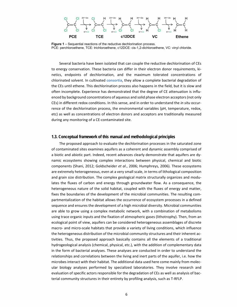
 Figure 1 – Sequential reactions of the reductive dechlorination process. PCE: perchloroethene, TCE: trichloroethene, c12DCE: cis-1,2-dichloroethene, VC: vinyl chloride.  

 

  Several bacteria have been isolated that can couple the reductive dechlorination of CEs 

to energy conservation. These bacteria can differ  in their electron donor requirements, ki‐

netics,  endpoints  of  dechlorination,  and  the  maximum  tolerated  concentrations  of 

chlorinated solvent. In cultivated consortia, they allow a complete bacterial degradation of 

the CEs until ethene. This dechlorination process also happens in the field, but it is slow and 

often incomplete. Experience has demonstrated that the degree of CE attenuation is influ‐

enced by background concentrations of aqueous and solid phase electron acceptors (not only 

CEs) in different redox conditions. In this sense, and in order to understand the in situ occur‐

rence of the dechlorination process, the environmental variables (pH, temperature, redox, 

etc) as well as concentrations of electron donors and acceptors are traditionally measured 

during any monitoring of a CE‐contaminated site.   

 

 

1.3. Conceptual framework of this manual and methodological principles

  The proposed approach to evaluate the dechlorination processes in the saturated zone 

of contaminated sites examines aquifers as a coherent and dynamic assembly comprised of 

a biotic and abiotic part. Indeed, recent advances clearly demonstrate that aquifers are dy‐

namic  ecosystems  showing  complex  interactions  between  physical,  chemical  and  biotic 

components (Shani, 2012; Goldscheider et al., 2006; Humphreys, 2006). These ecosystems 

are extremely heterogeneous, even at a very small scale, in terms of lithological composition 

and grain size distribution. The complex geological matrix structurally organizes and modu‐

lates  the  fluxes of  carbon and energy  through groundwater  flow. As a  consequence,  the 

heterogeneous nature of  the solid habitat, coupled with the  fluxes of energy and matter, 

fixes the boundaries of the development of the microbial communities. The resulting com‐

partmentalization of the habitat allows the occurrence of ecosystem processes in a defined 

sequence and ensures the development of a high microbial diversity. Microbial communities 

are able to grow using a complex metabolic network, with a combination of metabolisms 

using trace organic inputs and the fixation of atmospheric gases (lithotrophy). Then, from an 

ecological point of view, aquifers can be considered heterogeneous assemblages of discrete 

macro‐ and micro‐scale habitats that provide a variety of living conditions, which influence 

the heterogeneous distribution of the microbial community structures and their inherent ac‐

tivities.  Thus,  the  proposed  approach  basically  contains  all  the  elements  of  a  traditional 

hydrogeological analysis (chemical, physical, etc.), with the addition of complementary data 

in the form of bacterial analyses. These analyses are conducted in order to understand the 

relationships and correlations between the living and inert parts of the aquifer, i.e. how the 

microbes interact with their habitat. The additional data used here come mainly from molec‐

ular  biology  analyses  performed  by  specialized  laboratories.  They  involve  research  and 

evaluation of specific actors responsible for the degradation of CEs as well as analysis of bac‐

terial community structures in their entirety by profiling analysis, such as T‐RFLP. 

 7 

The original contribution of this methodology is the use of statistics derived from numerical 

ecology tools. These tools have been used successfully for many years in the general ecology 

analyses, and offer unrivaled analytical power  for complex data processing. The  tools  se‐

lected  in  this manual will  be mainly  used  for  the  analysis  of  the  physicochemistry  and 

bacteriological status of a contaminated aquifer; and the interpretations will be of value to 

understand existing degradation mechanisms. The conclusions drawn from the analysis will 

also help to identify the probable reasons for a halt in the reductive dechlorination process 

and to evaluate potential solutions. 

 

 

1.4. Keys for using the manual

  This document presents,  in detail, the proposed approach. The structure of the docu‐

ment  is  intended  for  a  user,  and  the  document  guides  the  interested  party  either  in 

"automatic" mode or in “step‐by‐step” mode for those who want to go deeper. Analyses of 

the bacterial communities involved in and interacting with the degradation of CEs are pre‐

sented, and a detailed case study  is described at  the end of  the manual. The appendices 

include all documents necessary for understanding and implementation of the procedure. 

For the numerical analysis, the necessary hardware is a simple desktop computer and a 

color printer. The software and connected libraries are open access and the detailed proce‐

dure script is provided in the appendices. 

 

 

1.5. Target audience

  This document is addressed to anyone involved in finding solutions for the remediation 

of aquifers contaminated with CEs. Basic knowledge of bacterial respiratory metabolisms and 

molecular biology will be useful to understand and carry out the proposed techniques. The 

use of  this manual also requires basic computer skills and some  familiarity with database 

management. Knowledge of basic statistics is strongly recommended, and knowledge of mul‐

tivariate statistics would be beneficial but is not specifically required. 

 

   

 8 

 

  2. OBJECTIVES  

 

  The objective of this manual is to offer a practical solution for anyone wishing to exam‐

ine, in detail, the remediation process (natural or enhanced) in a contaminated site, such as 

a saturated aquifer polluted by CEs. 

  First, a step‐by‐step screening tool for the evaluation of the site status and examination 

of the presence, or absence, of natural attenuation (NA) of the pollutants is presented. Sec‐

ond,  tools  are  presented  to  understand  the  potential  reasons  of  a  stalling  of  the  CE 

degradation process. Finally, the proposed tools can contribute to the choice of a remedia‐

tion technique or strategy and allow its monitoring in time and space. 

 

 

"How does it work?”

  The document presents a procedure based on a multivariate statistical tool dedicated 

to the analysis of data provided by geological, chemical and biological analyses. In this sense, 

aquifer ecosystem functioning is examined as a whole. The statistical analysis looks for the 

best correlation between different data sets and identifies the statistically significant varia‐

bles. A conceptual model of aquifer functioning regarding CEs degradation is deduced from 

the analysis. Interpretation of the model can then elucidate the possible stalling of lower CE 

degradation, and a corrective strategy can be proposed. 

  The protocol presented in this document can be implemented at different steps of the 

Swiss procedure  for  investigation of contaminated sites  (Diagram 1). This protocol can be 

inserted in the “detailed investigation” phase when the “specification of the technical inves‐

tigation”  is established and continued during the elaboration of the “remediation project” 

phase (FOEN, 2000; FOEN 2001a and b).The choice of the moment to apply the present meth‐

odology depends on the site, on the available equipment at the site (e.g. number of sampling 

wells), and also on technical and financial resources. 

 

 Diagram 1 - Systematic treatment of contaminated site in 4 phases (modified from FOEN, 2001a)  

   

 9 

 

  3. STEPS OF THE DIAGNOSTIC TOOL  

 

  GWSs are composed of both abiotic and biotic components, which are defined, respec‐

tively, as the “habitat” and “biota” i.e. the living organisms (Humphreys, 2006; Goldscheider 

et al., 2006). Evaluation of a site’s bioremediation potential is associated with an investiga‐

tion of habitat and biota components that can include multiple levels of analysis (Figure 2). 

Bacteria are targeted in biota as they are considered key actors in CE degradation (ChloroNet, 

2009) and biogeochemical cycles (Treseder et al., 2012; Rousk and Bengtson, 2014). Integra‐

tion of data obtained from the exploration of the different levels (Figure 2, e.g. hydrology, 

hydrochemistry, bacterial community, bacterial genes and enzymes) leads to an overall un‐

derstanding  of  the  system.  The  finest  appreciation  of  the  biological  functioning  and  CE 

degradation potential of a GWS will be obtained when the microbiology is characterized at 

every level and its interaction with abiotic environmental factors is analyzed.  

 

 

 Figure 2 – Groundwater system complexity associated to bioremediation strategy evaluations. A GWS is composed of habitat and biota components that can be analyzed at different levels, shown in the orange and blue boxes. The central circle of arrows indicates that dynamic interactions occur be-tween elements of the habitat and the biota, which are a driver of GWS functioning.. This diagram should be viewed as a snapshot of a real dynamic situation where all levels and components are interdependent.  

 

  On this basis, a step‐by‐step screening process is presented in Diagram 2. The procedure 

explores the potential for reductive dechlorination in an aquifer through three gradual steps 

(boxes in grey on the right of Diagram 2) that answer the following questions: 

1) Is in situ reductive dechlorination activity present? 

2) Is there potential for complete degradation? 

3) What are the reasons for possible incomplete reductive dechlorination in the aquifer? 

  Regarding the technical objectives (color boxes in Diagram 2), the first step is devoted to 

the acquisition of the key abiotic environmental data of the studied aquifer. The second step 

describes the characterization of microbiology directly and specifically involved in the reduc‐

tive dechlorination of CEs (levels of populations, activity of cells and functional genes; Figure 

2). The third step completes the analysis of microbiology at a wider scale (communities, Fig‐

ure 2) that includes not only reductive dechlorination but all bacterial activities of the aquifer. 

This last step also provides an integrated analysis of the results of microbiology and physico‐

 10 

chemistry inquiries (biota and habitat, respectively) to assess the global biogeochemical char‐

acteristics of the aquifer and their impact upon the biodegradation potential of CEs. 

 

 

 Diagram 2 – Systematic screening process, in three steps, for the evaluation of the potential of reductive dechlorination in an aquifer contaminated with chlorinated ethenes.  

 

 

   

 11 

 

4. ASSESSING IN SITU PRESENCE OF 

REDUCTIVE DECHLORINATION  

 

 Diagram 3 – The first step of the screening process for evaluation of the potential of biodegradation in aquifer contaminated with chlorinated ethene compounds.  

 

  The main objective of the first step of the procedure is to assess the presence or absence 

of reductive dechlorination inside the GWS. The different tasks to achieve this aim are de‐

tailed in Diagram 3. The first aspects to explore are related to the collection of groundwater 

chemistry data, with a particular interest in concentrations and distributions of PCE, TCE and 

their daughter degradation products, especially ethene, which is often not analyzed. Collec‐

tion of supplementary data about the geology, hydrology, and pedology of the site are also 

helpful (e.g. to give an overview of the water flow dynamic of the aquifer), as are data to 

evaluate the extent of the polluted area. Consequently, this examination of the site will result 

in a map of the contamination and the physicochemical data related to the studied aquifer 

habitat. 

 

 

4.1. Basis for the screening

  The “preliminary investigation” described in phase 2 of the procedure of contaminated 

site remediation enacted by the FOEN (1994 and 2001) provides preliminary conclusions for 

 12 

the first step of the current screening process (i.e. is dechlorination observed in situ and until 

which end products?). Whether the site must be remediated based on the findings of the 

“preliminary investigation” is continued in the FOEN procedure in phase 3 with a “detailed 

investigation” (Diagram 1). The “detailed investigation” aims to provide accurate information 

about the type and extent of pollution, as well as damage that is likely to be generated. These 

data are necessary for the authority to determine the urgency of remediation and its overall 

goals. It is at this stage that multiple steps from the current screening protocol can take place 

simultaneously. In some cases, some parts may already have started during the “technical 

field investigation” of step 3 of the “preliminary investigation” when the latter is needed to 

rank a site. 

 

 

4.2. Water sampling strategy or monitoring well network

  All sites are different, and there is no one standard way to start an investigation and to 

successfully achieve the desired objectives. FOEN (2003) has edited a well‐detailed assistance 

manual to delimit polluted sites and define sampling strategies (e.g. regarding the distribu‐

tion and the number of sampling points). The location and number of monitoring wells should 

be determined on a site‐specific basis. However, because monitoring wells are important pa‐

rameters  to  accurately  identify  contaminant  concentrations  and  determine  the  overall 

contribution of biological processes to contaminant decrease, these wells cannot be placed 

until sufficient knowledge of the aquifer system is obtained. Design of the monitoring net‐

work  will  be  determined  by  the  size  of  the  plume,  site  complexity,  source  strength, 

groundwater/ subsurface water interactions, direction of groundwater flow, hydraulic con‐

ductivity, etc. In all cases, a higher density monitoring network will yield a greater degree of 

confidence in the interpretation of the results. 

  For the current manual, screening of reductive dechlorination can be conducted through 

a one‐time sampling campaign where enough water is collected for completion of the whole 

procedure (see 5.2.1). Samples shall be taken in the saturated zone from different locations 

in the site schematically depicted in Figure 3: i) in the area of highest concentration, ii) along 

a down gradient from the contaminant "source" (if not yet eliminated) or from dense non‐

aqueous phase liquids (DNAPL), and iii) on a non‐impacted area allowing comparison of the 

geochemistry of uncontaminated groundwater with the contaminated plume. 

 

 

Figure 3 - Groundwater monitoring well network in an ideal plume of pollutant dispersion.  

 13 

  A total lower limit of 10‐12 monitoring wells representative of the locations described 

above is estimated to be enough to allow multivariate statistical analysis of the data. If data 

confidence limits cannot be reached with one‐time sampling campaign, for example due to 

fewer monitoring wells available on the site with no possibility to expand or because of ho‐

mogeneity of the data, two or more rounds of sampling can be planned with enough time 

between rounds (several months, see complete example in Shani et al. (2013)) to avoid rep‐

licates and allow evolution of the groundwater system parameters.  

 

 

4.3. Parameters to evaluate for appreciation of in situ state of reductive dechlorination

  The sequential  reductive dechlorination of the  initial contaminants PCE and TCE pro‐

duces well‐defined intermediates such as the more toxic c12DCE, the most toxic VC, and the 

harmless  end‐product  ethene  (Figure  1).  Formation  of  the  two  other  dichloroethenes, 

t12DCE and 1,1‐DCE, is also possible but rarely observed. During this process, which supports 

microbial growth, H2 is most often used as electron donor and the CEs as electron acceptors. 

H2 is typically supplied by the fermentation of organic substrates. PCE or TCE is reduced by 

the sequential loss of a chlorine atom, and presence of the daughter degradation products 

in a GWS unambiguously demonstrates that biological degradation occurs through the pre‐

dominant  reductive dechlorination process. This depends on many environmental  factors 

including strongly anaerobic conditions, presence of fermentable substrates for generation 

of molecular hydrogen, and the appropriate microbial populations to catalyze the reactions.  

 

4.3.1. Contaminant map

  For the 1st step, the concentrations related to the pollutant and degradation products 

that must be measured are marked with * (the others are optional): 

PCE* and TCE* normally the initial contaminants of the site, and highly recalcitrant 

to oxidation. Their degradation only occurs in strictly anaerobic conditions. TCE can 

also be degraded by co‐metabolism in aerobic conditions (see section 5, Figure 6) but 

with low efficiency. This is considered a minor degradation pathway. 

c12DCE*, t12DCE, 11DCE among the DCE isomers, c12DCE is the main intermediate 

product of the reductive dechlorination process (more than 80%). Concentrations of 

t12DCE and 11DCE are generally low.  

VC* under reductive conditions (i.e. allowing sulfate reduction or methanogenesis, 

see 4.1) DCE  is degraded to form VC, a carcinogenic compound, with much higher 

toxicity than the parent molecules PCE and TCE. 

Ethene* is the harmless end product of reductive dechlorination and the best indi‐

cator  for  the  presence  of  a  complete  reductive  dechlorination  process  in  the 

saturated zone of a GWS.  

Chlorides (Cl‐) are the end products of both biotic and abiotic degradation of CEs.  

 

  The analytic methodology for measurement of CEs in solid and aqueous samples is pre‐

sented  in FOEN (2013), under methods S‐8 and E‐8, respectively (Appendix 2). Ethene and 

ethane can be measured with the methodology proposed by Kampbell et al.,  (1989), and 

chlorides can be measured using ion chromatography. 

Results of the measured concentrations are then evaluated with respect to permis‐

sible concentration limits listed in the Federal Ordinance on the Remediation of Polluted Sites 

(Table 1, Appendix 1 of OSites 814.680 available at http://www.admin.ch/opc/fr/classified‐

 14 

compilation/19983151/index.html). Aquifer zones with concentrations above the limits are 

mapped, and the PCE/TCE/daughter product distribution along the contaminant plume may 

be interpreted with the help of hydrogeological data collected from the site. 

 

 Table 1 - Overview of contaminant concentration limits (mg/L) presented in the Federal Ordinance on the Remediation of Polluted (OSites 814.680) and other guidance and limit values

Contaminant Concentration Limit value Limit value Limit value OSites OSEC OMS US-EPA water drinking water drinking water drinking water Perchloroethene 0.04 0.04 0.04 0.005 Trichloroethene 0.07 0.07 0.02 0.005 Cis-1,2-dichloroethene 0.05* 0.05* 0.05* 0.07 Trans-1,2-dichloroethene 0.05* 0.05* 0.05* 0.1 1,1, dichloroethene 0.03 0.03 - 0.007 Vinyl chloride 0.0001 - 0.0003 0.002

Modified from Chloronet, 2009. OSEC: Ordinance on foreign substances and components, OMS: World health organ-ization, US-EPA: US Environmental Protection Agency. * Limit value referring to the sum of cis and trans-1,2-dichloroethene.

 

 

4.3.2. Interpretation of contaminant concentrations and detected end products

  The investigation of contaminant concentrations leads to different conclusions based on 

which CEs, including ethene, are detected. (Diagram 3).  

  The detection of ethene indicates that the potential for complete reductive dechlorina‐

tion of PCE/TCE is already present in situ. The detection of only DCE and/or VC as degradation 

end products indicates an incomplete anaerobic degradation process. No detection of eth‐

ene, VC or DCE reveals an absence of in situ reductive dechlorination activity.   

  The finding of incomplete in situ reductive dechlorination has already been observed at 

several PCE/TCE contaminated sites, and has been attributed to different factors, including: 

i) insufficient anaerobic conditions to support reductive dechlorination activity, ii) a lack/ab‐

sence  of bacterial  populations  capable  of  reductive  dechlorination  of  c12DCE  to VC  and 

ethene (Lorah and Voytek, 2004; Dowideit et al., 2010 ), and iii) a lower reaction rate of the 

last steps of the sequential degradation process that create an apparent accumulation of DCE 

and/or VC (Middeldorp al., 1999; Figure 1). The reasons why PCE/TCE dechlorination is not 

detected or  is  incompletely  realized  in situ, with apparent or actual accumulation of DCE 

and/or VC, will be evaluated in the next steps of this screening procedure. 

  Further from the contaminant source, VC and c12DCE can migrate  into aerobic areas 

(Figure 5) where direct oxidation of this compound can occur and produce CO2 (Figure 6). 

This indicates that remediation can be achieved by different, successive processes depending 

on the conditions. To avoid misinterpretation of a non‐detection of ethene, stability of the 

site hydrochemistry should be monitored (FOEN, 2004) and degradation rates should be eval‐

uated.  The  case  where  ethene  production  is  measured  in  situ,  determines  whether  a 

monitored natural attenuation (MNA) strategy for remediation of the site is possible. MNA 

as remediation alternative can be proposed upon the confirmation that the transformation 

processes are taking place at a rate protective of human health and the environment. The 

evaluation should include a reasonable expectation that these processes will continue at an 

acceptable rate for an acceptable period of time (EPA, 1999; EPA, 1998). This last evaluation 

and determination of success are not further dealt with in this protocol; however literature 

has been published on this subject (EPA, 1998; Chapelle et al., 2003; ADEME, 2007; Grandel 

et Dahmke, 2008, Umweltbundesamt, 2011).  

 

 15 

 

4.4. Parameters for evaluation of GWS physicochemistry and redox conditions

 

4.4.1. Predominant terminal electron-accepting processes

  A reliable approach  for screening bacterial degradation potential of CEs relies on the 

identification of the predominant Terminal Electron‐Accepting Processes (TEAPs) occurring 

in a GWS (Chapelle et al., 1995). TEAPs are related to the bacterial oxidative/reductive respi‐

ration processes. In any environment in which microbial activity occurs, there is a progression 

from oxic to anoxic conditions, and different bacteria along this progression use a specific 

sequence of compounds as terminal electron acceptors for respiration. Under aerobic condi‐

tions, oxygen  is the final electron acceptor. In the absence of oxygen, bacteria are able to 

transfer electrons to other oxidized inorganic compounds (e.g. NO3‐, SO4

2‐) and use them as 

terminal electron acceptors. To illustrate this, Figure 4 presents a schematic view of the se‐

quential TEAPs defining aquifer oxidation/reduction conditions: reactions 1 to 6 correspond, 

respectively,  to aerobic  respiration, denitrification  including nitrate  reduction, manganese 

reduction, iron reduction, sulfate reduction and methanogenesis. Each reaction happens suc‐

cessively  in the previously stated order, and once an electron acceptor  is depleted, a new 

redox reaction using another acceptor occurs. The electron acceptor that leads to the next 

largest generation of energy during the reaction will dominate (EPA, 2000; Figure 4, right). 

Consequently, this succession of respiring oxidative/reductive processes (TEAPs) affects the 

chemistry and redox conditions of groundwater in all aquifer systems.  

  Each respiring process occurs in a specific redox potential (Eh) range, which decreases 

from aerobic respiration until methanogenisis (Figure 4, left).  The processes also require, as 

electron donors, different ranges of dihydrogen concentrations (or an equivalent reducer) 

(Figure 4, right). 

  In this context, the occurrence of CE reductive dechlorination depends on redox condi‐

tions of the aquifer established by the inhabiting bacterial populations implicated in TEAPs 

and  the  availability  of  inorganic  electron  acceptor  compounds  along  the  contamination 

plume (Figure 5). Reductive dechlorination occurs from a specific redox potential slightly less 

than that of denitrification (Figure 4, in green) and within the required specific ranges of di‐

hydrogen availability.  

  When the redox potential, Eh, is approximately 500 mV, PCE will be degraded to VC with 

a  low concentration of reducing equivalents (<1 nM H2). The required reducing equivalent 

concentration is higher to reduce VC to ethene (>1‐10 nM H2). Other TEAPs with lower redox 

potentials (e.g. manganese reduction) take advantage of this high requirement and can out‐

compete  the VC  reduction process because  they  require  lower concentrations of  reducer 

equivalent (<1 nM H2). Conversely, the dechlorination process competes for electron donors 

with  bacterial  TEAPs  that  require  the  same  concentration  range  of  dihydrogen,  such  as 

c12DCE  reduction and manganese  reduction. Competition also occurs when  low  reducing 

conditions are achieved in the aquifer, as in the case of VC dechlorination competition with 

sulfate reduction and methanogenesis for reduction equivalents. 

 

 16 

Figure 4 – Ecological succession of terminal electron acceptor processes (TEAPs) linked to bacterial respiring processes. 1) Aerobic respiration, 2) Denitrification, 3) Manganese reduction, 4) Iron reduction, 5) Sulfate reduction 6) Methanogenesis. Oxidation-reduction potentials of the reactions are shown on the left (Eh in Volts). Ranges of dihydrogen concentrations required for each TEAP are shown on the right. Reductive sequen-tial CE dechlorination processes are depicted in green. Organic matter degradation pathways providing equivalent reducing potential in the system are schematized in the blue flow scheme at the top of the figure.  

 

  The reductive dechlorination process is included in the ecological succession of TEAPs. 

Consequently, determining TEAPs that occur in an aquifer, documenting their spatial distri‐

bution, and understanding how they affect concentrations of contaminants are central to 

assess and predict the possibilities of CE dechlorination.  

  The distribution of TEAPs in a GWS can be assessed by measuring the availability of elec‐

tron acceptors  (e.g. NO3‐, Mn(IV), Fe(II), SO4

2‐) and/or by showing the distribution of their 

reduced forms (e.g. NO2‐, Mn(II), Fe(II), S2‐/H2S). For this purpose, some important parame‐

ters need to be measured to complement the CE concentration measurements. 

 

4.4.2. Parameters to evaluate the redox conditions of the GWS

In the current procedure, details regarding the necessary parameters are given to clarify the 

existing data acquisition methodology. The relative procedures and documentation for data 

acquisition are available in the following documents: 

1)  Sampling of groundwater in relation to contaminated sites (FOEN, 2003) 

2)  Analytical methods in the field of waste and polluted sites (FOEN, 2013)  

3) Contaminated sites, evaluation of risk. Specifications for the technical  investiga‐

tion of contaminated sites (FOEN, 2000)   

4)  Practical guidelines for the protection of groundwater (FOEN, 2004) 

For the water sampling procedure, see Section 5.2.1. Again, it  is important to note that all 

water samples needed throughout the whole screening procedure must be collected at the 

same time to obtain results that can be analyzed in a comprehensive and integrative way. 

 17 

Figure 5 ‐ Redox zones of a typical contaminant plume. 

A plume moving with groundwater flow will typically develop distinct redox zones. In a conceptual con-taminant plume, a “redox gradient” is established due to dilution from the source, movement of CEs with groundwater flow, and microbial activities (i.e. TEAPs).  

 

4.4.2.1. General parameters and descriptions

Essential parameters, which must be measured, are marked below with *. Others are com‐

plementary and useful, but not essential: 

Oxidation/reduction potential * (ORP): “Redox” potential is directly measured by a field 

electrode device. Eh  is the ORP value corrected relative to the standard hydrogen elec‐

trode. 

pH *: pH has a great  impact on dechlorinating microorganisms. For example, KB‐1TM a 

natural dechlorinating microbial consortium that contains phylogenetic relatives of Deha‐

lococcoides ethenogenes  (Major et al., 2002), did not show any dechlorination activity 

below pH 5 or above pH 10, optimum pH for dechlorination being between 6.0 and 8.0. 

Temperature *: Lower temperatures limit dechlorination activity 

Electrical conductivity * (eC): eC indicates global ion concentration in solution. 

Dissolved oxygen * (dO2): Dissolved oxygen is the electron acceptor used by aerobic mi‐

croorganisms  to  degrade  organic matter.  Anaerobic  bacteria  are  inhibited  by  an  O2 

concentration higher  than 0.5 mg/L, and  reductive dechlorination cannot occur  in  this 

condition. When dO2 decreases due to organic matter respiration, anaerobic bacteria suc‐

cessively  use  other  electron  acceptors  for  respiration  as  indicated  in  Figure  4.  Each 

terminal electron acceptor, when used, modifies the groundwater’s ORP status, and en‐

vironmental redox conditions become more and more reduced.  

 

  ORP/Eh, pH, temperature, conductivity and dO2 measurements are obtained in the field 

using portable electric power units. These parameters are standard for groundwater quality 

analysis (Appendix 1) and are not specific to contaminated site investigations.  

 

4.3.2.2. Chemical parameters

nitrate NO3‐ * , nitrite NO2‐*, ammonium NH4

+ : Nitrogen is found in groundwater as dis‐

solved organic nitrogen, NO3‐, NO2

‐ or NH4+. Low concentrations of NO3

‐ in saturated zones 

indicate possible anaerobic bacterial respiration like dissimilatory nitrate reduction to ni‐

trite (NR) and denitrification (NO3‐ > NO2

‐ >>> N2). Denitrification takes place at oxic/anoxic 

 18 

interfaces, as part of the NO3‐ along a soil profile comes from leaching and microbial oxi‐

dation of NH4+, called nitrification (NH4

+ > NO2‐ > NO3

‐), which occurs  in the upper oxic 

environment. NO3‐ are considered as weakly available at concentrations below 1 mg/L. 

Under NO3‐ depleted conditions, reductive dechlorination of PCE to TCE can occur. NO2

‐ is 

an intermediate of both denitrification and nitrification, which are respectively anaerobic 

and aerobic processes. Thus, the presence of NO2‐ at oxic/anoxic  interfaces (i.e. slightly 

reducing  conditions)  can  indicate  either  incomplete denitrification  (stopped  after NR) 

and/or  incomplete nitrification  (stopped after oxidation of ammonium). This  situation 

must be  interpreted with  caution  and  in  relationship  to other measured parameters. 

When  anaerobic  redox  conditions  (i.e.  strongly  reducing)  are  combined  with  high 

amounts of carbon, bacteria may reduce NO3‐ to NH4

+ by dissimilatory nitrate reduction 

to ammonium (DNRA). Nevertheless, NH4+ is found naturally in GWSs as a result of anaer‐

obic decomposition of organic material (Böhlke et al., 2006), and high NH4+ concentrations 

are a common sign that surface water influenced by anthropogenic activities is infiltrating 

to  groundwater  (Lindenbaum,  2012). Consequently,  interpretation of NH4+  concentra‐

tions in a GWS must also be done with caution. 

reduced manganese Mn(II) *: An Mn(II) measurement is indicative of manganese(IV) re‐

duction. Manganese(IV) reduction is restricted to conditions where SO42‐ concentrations 

are low or absent (EPA, 1999). Redox conditions of Manganese(IV) reduction are favorable 

for and in competition with DCE to VC degradation since the same H2 concentration range 

is required for both reactions (MacMahon et al., 2008; Figure 4). 

reduced  iron  Fe(II) *: When manganese oxides become  limiting,  iron(III)  reduction  to 

iron(II) is the predominant TEAP. It seems that iron reduction doesn’t occur until all Mn(IV) 

oxides  are  depleted. When  groundwater  is  under  iron  reducing  conditions,  reductive 

dechlorination of PCE and TCE to c12DCE and VC is possible (Figure 4, same range of re‐

quired H2 concentrations). 

sulfate SO42‐ *: When SO4

2‐ become the main electron acceptor, redox conditions are re‐

duced  and  complete  reductive dechlorination  (PCE  until  ethene)  is  possible.  The  EPA 

technical protocol for evaluating NA (EPA, 1998) indicates that SO42‐concentrations must 

be  lower  than 20 mg/L  to avoid competition between sulfate  reduction and  reductive 

dechlorination. 

sulfide H2S *(S2‐ ): S2‐ is a dissolved gas and a product of sulfate reduction. Sulfides easily 

react and precipitate with metal ions such as ferrous iron and can therefore be difficult to 

measure in some GWSs. 

methane CH4 *: Stable molecule and easily  to measured methane  indicates highly  re‐

duced  conditions  characteristic  of  methanogenesis  and  favorable  for  reductive 

dechlorination. Methanogenesis can be observed even if SO42‐ is not depleted. The EPA 

protocol asserts that a methane concentration higher than 1 mg/L indicates competition 

between methanogenesis and reductive dechlorination and leads to VC accumulation on 

site.  

carbon dioxide CO2 *: CO2 is an oxidized electron acceptor of methanogenesis and also 

an end product of CE oxidation (see section 5, Figure 6).  

total organic carbon  (TOC) * and chemical oxygen demand  (COD):   TOC and COD are 

evaluations of the global carbon content in groundwater. The non‐purgeable organic car‐

bon  (NPOC)  measurement  procedure,  which  includes  few  or  no  volatile  organic 

compounds, must be used to prevent organochlorine compounds  from contributing to 

the measured value. Measurement of organic carbon content is linked to the evaluation 

of available electron donors (reducer equivalents) in a GWS for the TEAPs (Figure 4, blue 

 19 

boxes) that  lead aquifers to optimal, anaerobic conditions for biodegradation of CEs. A 

low TOC concentration will contribute to a lower efficiency of CE biodegradation. 

   

 20 

 

5. POTENTIAL FOR REDUCTIVE 

DECHLORINATION OF CES  

 

 Diagram 4 - Second step of the screening process for the evaluation of the reductive dechlorination potential in an aquifer contaminated with chlorinated ethenes.  

 

  In  this  step,  the  bacteria  implicated  in  the  reductive  dechlorination  processes,  the 

organohalide‐respiring bacteria (OHRB), are studied directly from water or aquifer sediment 

samples. The general objective is to evaluate the inherent potential  for biological reductive 

dechlorination of CEs in a GWS (Diagram 4). 

The proposed analysis determines whether OHRB are present, and  if so then assesses 

whether  they  express  the  ability  to  completely  dechlorinate  CEs.  This  is  achieved  by 

completing the following technical objectives: 

Detect, with molecular  tools,  the presence of bacteria and enzymes known  to be 

involved in the process of reductive dechlorination 

Assess the intrinsic capacity of aquifer samples to express the biochemical activities 

of reductive dechlorination through microcosm tests 

 

  The results obtained from completion of these two objectives can clarify observations 

made during step 1. For example, they may indicate that incomplete degradation is due to 

the absence of some OHRB and/or the lack of the enzymatic machinery required for complete 

dechlorination (Diagram 4, grey boxes). 

 21 

 

5.1. Looking for biomarkers in aquifer samples: Organohalide-respiring bacteria and re-ductive dehalogenase genes detection

 

5.1.1. Biodegradation processes of chlorinated-ethenes (Bradley, 2003)

  Different bacterial processes are implicated in CE degradation (Figure 6):  

1) Metabolic processes are those in which CEs are used as electron acceptors in reductive 

dechlorination in the saturated zone (see also, Figure 1) or as electron donors in oxidation 

reactions (oxidative pathway) used to obtain energy and produce biomass. Aerobic oxida‐

tion of VC occurs at a higher rate than anaerobic reductive dechlorination. VC oxidation may 

be  important  in downstream aerobic areas, where a GWS’s redox conditions return to  its 

natural state (Figure 5).  

2) Co‐metabolic processes are defined as reactions in which a non‐specific enzyme produced 

for microbial metabolism fortuitously reduces a chlorinated molecule. No benefit returns to 

the implicated microorganisms.  

3) Anaerobic oxidation processes are those  in which VC and DCE can be directly oxidized 

under  iron‐ and manganese‐reducing conditions, respectively. Alternatively, VC can be de‐

graded into acetate via oxidative acetogenesis. The produced acetate can be mineralized to 

CO2 and CH4 through acetoclastic methanogenesis and to CO2 via microbial humic acids re‐

duction. It can also be used as an electron donor and/or carbon source by other anaerobic 

bacterial processes, i.e. TEAPs including reductive dechlorination. 

 

 

Figure 6 – Bacterial reductive and oxidative processes for degradation of chloroethenes (CEs). Electrons donors are shown in orange, and electrons acceptors in blue. PCE: perchloroethene, TCE: trichloroethene, cDCE: cis-1,2-dichloroethene, VC: vinyl chloride, Cl-: chloride, NO3

-: nitrate, NH4+: am-

monium, CH4: methane.  

 

  The abiotic pathway is a 4th type of process where CEs are reduced by chemical reaction 

with active compounds. Abiotic agents that may enhance the dechlorination of CEs are zero‐

valent metals, sulfide minerals or green rusts  (Tobiszewski and Namiesnik, 2012). Natural 

abiotic dechlorination occurs rarely and is slower than bacterial reductive dechlorination. 

  It  is not possible to distinguish the four reactions  in the field. Nevertheless, reductive 

dechlorination of CEs by organohalide respiration (OHR) (Figure 7‐B) does occur in the anoxic, 

saturated zones of an aquifer. This pathway was demonstrated and is recognized as the most 

 22 

efficient CE degradation process that takes place in contaminated aquifers (Chloronet, 2009; 

EPA, 2000). 

 

 

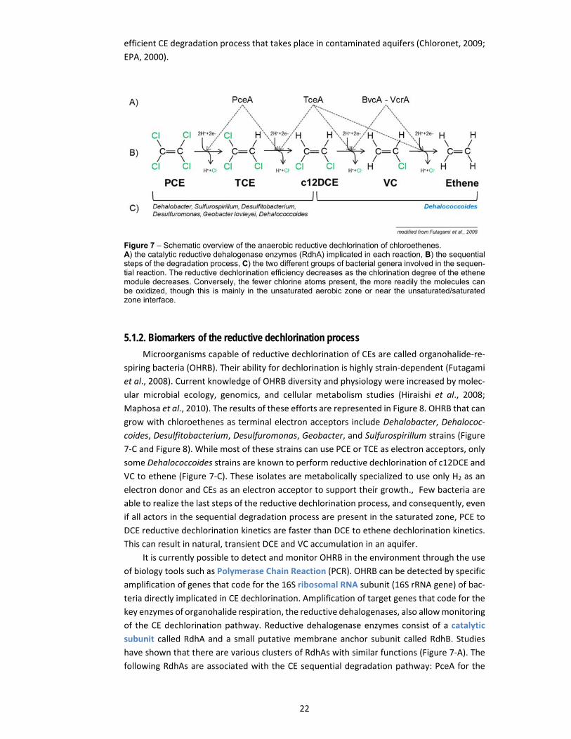
 Figure 7 – Schematic overview of the anaerobic reductive dechlorination of chloroethenes. A) the catalytic reductive dehalogenase enzymes (RdhA) implicated in each reaction, B) the sequential steps of the degradation process, C) the two different groups of bacterial genera involved in the sequen-tial reaction. The reductive dechlorination efficiency decreases as the chlorination degree of the ethene module decreases. Conversely, the fewer chlorine atoms present, the more readily the molecules can be oxidized, though this is mainly in the unsaturated aerobic zone or near the unsaturated/saturated zone interface.  

 

5.1.2. Biomarkers of the reductive dechlorination process

  Microorganisms capable of reductive dechlorination of CEs are called organohalide‐re‐

spiring bacteria (OHRB). Their ability for dechlorination is highly strain‐dependent (Futagami 

et al., 2008). Current knowledge of OHRB diversity and physiology were increased by molec‐

ular microbial  ecology,  genomics,  and  cellular metabolism  studies  (Hiraishi  et  al.,  2008; 

Maphosa et al., 2010). The results of these efforts are represented in Figure 8. OHRB that can 

grow with chloroethenes as terminal electron acceptors  include Dehalobacter, Dehalococ‐

coides, Desulfitobacterium, Desulfuromonas, Geobacter, and Sulfurospirillum strains (Figure 

7‐C and Figure 8). While most of these strains can use PCE or TCE as electron acceptors, only 

some Dehalococcoides strains are known to perform reductive dechlorination of c12DCE and 

VC to ethene (Figure 7‐C). These isolates are metabolically specialized to use only H2 as an 

electron donor and CEs as an electron acceptor to support their growth.,  Few bacteria are 

able to realize the last steps of the reductive dechlorination process, and consequently, even 

if all actors in the sequential degradation process are present in the saturated zone, PCE to 

DCE reductive dechlorination kinetics are faster than DCE to ethene dechlorination kinetics. 

This can result in natural, transient DCE and VC accumulation in an aquifer. 

  It is currently possible to detect and monitor OHRB in the environment through the use 

of biology tools such as Polymerase Chain Reaction (PCR). OHRB can be detected by specific 

amplification of genes that code for the 16S ribosomal RNA subunit (16S rRNA gene) of bac‐

teria directly implicated in CE dechlorination. Amplification of target genes that code for the 

key enzymes of organohalide respiration, the reductive dehalogenases, also allow monitoring 

of the CE dechlorination pathway. Reductive dehalogenase enzymes consist of a catalytic 

subunit called RdhA and a  small putative membrane anchor  subunit called RdhB. Studies 

have shown that there are various clusters of RdhAs with similar functions (Figure 7‐A). The 

following RdhAs are associated with the CE sequential degradation pathway: PceA for the 

 23 

tetrachloroethene  reductase, TceA  for  the  trichloroethene  reductases and BvcA and VcrA 

both for DCE and vinyl chloride reductases (Futagami et al., 2014; Maphosa et al., 2010).

 

 

Figure 8 – Phylogenetic tree of organohalide respiring bacteria based on bacterial 16S rRNA gene se-quences. The reference bar at the bottom center indicates the branch length that represents 10% sequence diver-gence. Electron donors and acceptors are listed in the text boxes and are grouped according to their chemical nature and complexity. Color key: Chloroflexi (red), Deltaproteobacteria (blue), Epsilonproteo-bacteria (purple), Firmicutes (green). Abbreviations: CF, chloroform; DCA, dichloroethane; DCE, dichloroethene; HCH, hexachlorocyclohexane; PCB, polychlorinated biphenyls; PCE, tetrachloroethene; TCE, trichloroethane; TCA, trichloroethene; VC, vinyl chloride.  

 

5.2. Evaluation for potential of reductive dechlorination by specific detection of the pres-ence of known OHRB and reductive dehalogenase genes

  At this stage, the proposed analyses are carried out on DNA extracts from water sam‐

ples. Results  of  this  first molecular  analysis will  indicate  the  presence of bacterial  guilds 

implicated in reductive dechlorination. These data can be obtained relatively rapidly, how‐

ever the presence of bacteria does not mean that they are or could be active. Regarding the 

molecular investigation of bacterial activity, one path is to analyze gene expressions by tar‐

geting messenger RNA (mRNA) that code for proteins and the enzymatic machinery of the 

cell. This investigation yields data closer to the real activity than DNA analysis, but is more 

expensive  in terms of  laboratory materials and more complicated  in terms of technical ex‐

pertise in molecular biology. The choice to work on DNA is made to facilitate the knowledge 

transfer. The data obtained with this  investigation are powerful for evaluation of a GWS’s 

dechlorination potential, and extensive experiments can be realized at any time. 

 

 

 

5.2.1. Water sampling: collection, transportation and storage.

 24 

  The general procedure  for  sampling contaminated groundwater  is currently well de‐

scribed (FOEN, 2013; EPA, 2008). Biology‐specific analyses are detailed in Shani (2012). Water 

samples for microbial analysis must be collected at the same time as the water samples for 

chemical analysis in the 1st step of the screening procedure. Groundwater samples are col‐

lected using a peristaltic pump (e.g. Type P2.52, Eijkelkamp, Giesbeek, The Netherlands) and 

PTFE tubes (inner diameter 4 mm, Semadeni SA, Switzerland). Each well is purged at a flow 

rate of 100 mL/min, and physicochemical parameters (temperature, pH, electrical conductiv‐

ity, ORP) are continuously measured through a flow cell device. Purging lasts for at least one 

well  volume  and  continues  until  the  physicochemical  parameters  stabilize. Groundwater 

samples are then collected from each well directly at the pump exit at the low flow rate of 

100 mL/min. Water  is sampled  for chemical analysis (FOEN, 2013), and 1 L  is sampled  for 

molecular biology analyses by completely filling a 1 L polypropylene Nalgene® bottle (Thermo 

Fisher Scientific, USA) without headspace. For microcosm experiments, two sterile 40 mL se‐

rum glass vials (type 27051 SUPELCO, Sigma‐Aldrich, Buchs SG, Switzerland) are filled with 

water and hermetically sealed to avoid sample contact with air. After collection, aqueous 

samples should be protected from light and refrigerated for transport from the field. In the 

laboratory, all groundwater samples are stored in the dark and at 4°C until analysis, which 

should be done immediately or within a maximum of 48 hours after sampling.  

 

5.2.2. Sample filtration and DNA extraction

  Groundwater samples are filtered under a  laminar  flow hood with a  filtration system 

(Filter Funnel Manifolds, Pall Corporation, USA) and a 0.2 µm pore size, sterile polycarbonate 

membrane (IsoporeTM Membrane Filters, Millipore, USA) or with Nalgene® bottle‐top sterile 

filter units (Sigma‐Aldrich, Buchs SG, Switzerland). The complete water sample volume of 1 L 

should be filtered. Several membranes can be used if necessary, then stored in a sterile con‐

tainer. Following filtration, membranes are submitted to DNA extraction using the protocol 

detailed in Appendix 3 or kept at ‐20°C for long term storage. 

 

5.2.3. PCR specific detections of OHRB and RdhA genes

  As mentioned previously, the specific PCR detection of OHRB 16S rRNA genes and genes 

associated with the catalytic subunit of reductive dehalogenase (RdhA) are indicative of the 

presence of bacterial guilds involved in CE reductive dechlorination. Presence of OHRB and 

related genes is assessed by PCR amplifications with the primers listed in Table 2 by following 

the protocol in Appendix 4. 

 

 

5.3. Evaluation of the intrinsic reductive dechlorination potential of a GWS using micro-cosm experiments

  In this 2nd phase of the 2nd step of the procedure (Diagram 4), groundwater samples are 

placed in optimal conditions for the biochemical expression of reductive dechlorination. All 

or some intermediate compounds of degradation (TCE, DCE, VC and ethene) will be produced 

according  to  the OHRB guilds presents  in  the water  sample. The complete procedure  for 

preparation of microcosms is detailed in Appendix 5. Briefly, the anaerobic medium is pre‐

pared as detailed  in Holliger et al.,  (1993) except that  fermented yeast extract solution  is 

replaced by 0.1 g/L of peptone. For the preparation of one microcosm, 5 mL of PCE dissolved 

in hexadecane (100mM) are added to 50 mL of sterilized anaerobic medium. Through a 0.2 

µm  filter, 1 mL of electron donor mixture  (equal parts ethanol, butyrate, and propionate, 

 25 

each at 100mM) is also added. The gas phase in the microcosm is aseptically changed with 

N2/CO2 (4:1, vol/vol) before the final step of inoculation with 5 mL of groundwater sample. 

The microcosms are incubated in the dark at 30°C for at least 3 months. The gas phase in the 

microcosm  is  sampled  regularly and analyzed with GC  for  the presence of dechlorination 

products TCE, DCE, VC, and ethene. 

 

 Table 2 - Organisms and genes specifically targeted to evaluate reductive dechlorination potential.  

Target organism/gene Primer Sequence (5’-3’) References

Dehalococcoides sp. * DHC587f GGACTAGAGTACAGCAGGAGAAAAC Hendrickson et al., 2002 DHC1212r GGATTAGCTCCAGTTCACACTG ‘’ Dehalobacter sp.* Dre441f GTTAGGGAAGAACGGCATCTGT Smits et al., 2004 Dre645r CCTCTCCTGTCCTCAAGCCATA ‘’ Sulfurospirillum sp. * DHSPM576f GCTCTCGAAACTGGTTACCTA Ebersole et al., 2003 DHSPM1210r GTATCGCGTCTCTTTGTCCTA ‘’ Desulfuromonas sp. * Desulfo494f AGGAAGCACCGGCTAACTCC Bond et al., 2002 Desulfo1050r CGATCCAGCCGAACTGACC ‘’

Desulfitobacterium sp.* Dsb406f GTACGACGAAGGCCTTCGGGT Smits et al., 2004 De2r CCTAGGTTTTCACACCAGACTT Lanthier et al., 2001 Geobacter lovley Geo73f CTTGCTCTTTCATTTAGTGG Duhamel and Geo485r AAGAAAACCGGGTATTAACC Edwards, 2006 vcrA ** vcrA880f CCCTCCAGATGCTCCCTTTA Behrens et al., 2008 vcrA1018r ATCCCCTCTCCCGTGTAACC ‘’ bvcA** bvcA227f TGGGGACCTGTACCTGAAAA ‘’ bvcA523r CAAGACGCATTGTGGACATC ‘’ Eubacteria 27f AGAGTTTGATCMTGGCTCAG Lane 1991 519r GWATTACCGCGGCKGCTG Turner et al., 1999

* gene coding for the small 16S ribosomal RNA subunit (16S rRNA gene) is targeted to specifically detect the mentioned bacterial genus. ** genes coding in Dehalococcoides sp. for the reductive dehalogenase enzymes implicated in the dechlorination of c12DCE into VC then ethene.

 

 

5.4. Basis for interpretation of the microbial analyses

  Whether there is biochemical potential for complete dechlorination can be elucidated 

from the presence or absence of OHRB and the RdhA genes. This is particularly important if, 

in step 1 of the procedure, the in situ contaminant concentrations show that PCE and/or TCE 

are  not  degraded  or  that  the  degradation  is  incomplete with  observed  accumulation  of 

c12DCE and/or VC. Several scenarios may occur: 

  a)  If the tested biomarkers are not detected,  in particular the genus Dehalococcoides 

and the RdhA genes, the biochemical potential required for complete dechlorination is miss‐

ing  (Diagram  4,  grey  box).  If  microcosm  experiments  also  show  an  inability  to  induce 

complete dechlorination of PCE, it can be concluded that an accumulation of c12DCE and/or 

VC will occur. 

  b) Conversely, the whole set of biomarkers may be not detected in PCR while a biochem‐

ical  potential  for  complete  degradation  is  observed  in  microcosms.  Like  any  other 

measurement  technique, PCR has  a detection  threshold. A negative PCR  result does not 

prove the absence of the target; it can indicate a quantity that is too low to be detected. This 

undetected potential by molecular tools would be revealed through the microcosm experi‐

ments. 

A positive result from microcosm experiments could also suggest that the potential for 

dechlorination exists at the tested site, but that it is carried out by yet unknown bacteria and 

genes not  targeted by  the PCR analysis. Currently only  some Dehalococcoides  strains are 

 26 

known to completely dechlorinate PCE to ethene (Figure 7‐C), and the reductive dechlorina‐

tion  process  appears  to  be  accomplished  by  bacterial  consortia where  each  population 

performs one or several of the sequential dechlorination steps (e.g. Holliger and Schumacher, 

1999; Gu et al., 2004 Yang et al., 2005). Complete dechlorination of CEs has been observed 

without evidence of usually “wanted” biomarkers, especially Dehalococcoides strains (Flynn 

et al., 2000). This suggests that consortia of non‐Dehalococcoides dechlorinating strains can 

achieve  complete dechlorination, and moderation  is advised  regarding  the assertion  that 

Dehalococcoides strains are necessary for complete dechlorination.  

  c) Another possible case is detection of all or part of the biomarkers using PCR with no 

activity exhibited in microcosm experiments. This result suggests that microorganisms asso‐

ciated with the targeted biomarkers do not have functional enzyme systems or that  items 

are missing for sequential dechlorination steps (Diagram 4, grey box).   

  d)  In the  last case, all tested biomarkers may be detected,  including OHRB and RdhA 

genes (Figure 7‐A), and complete reductive dechlorination may have been induced in micro‐

cosm experiments. This is a reliable indication that the necessary biochemistry is present in 

the tested GWS to realize complete dechlorination.  If the whole process was not observed 

in situ during analysis in step 1, it could be because the redox conditions of the tested aquifer 

are not yet favorable for reductive dechlorination or an inherent problem linked to the struc‐

ture of the aquifer exists. These latter aspects will be specifically investigates in step 3 of the 

screening procedure. 

 

   

 27 

 

6. AQUIFER BIOGEOCHEMISTRY  

 

 Diagram 5 - Third step of the screening process for the evaluation of the dechlorination potential in aquifers contaminated with chlorinated ethenes.  

 

  In  this  step,  reductive  dechlorination  processes  are  placed  in  the  framework  of 

interactions with other natural bacterial processes (TEAPs) occurring in a GWS. The general 

objective  is to evaluate the reasons why the reductive dechlorination of CEs  is perturbed, 

usually observed in situ by the absence of ethene production and stalling of the degradation 

process at c12DCE and/or VC (Diagram 5). 

  The technical objective of this 3rd step is the analysis of the global bacterial community 

that lives  in and  interacts with the aquifer habitat (Figure 2) and also supports OHRB guild 

activities. For this community fingerprinting, a molecular method is used and provides mul‐

tiple  useful  “barcode”  characteristics  of  the  bacterial  community  structure  (BCS)  at  the 

different sampling locations. Raw data from the descriptions of the habitat (output of step 1) 

and the biota (outputs of step 2 and 3) are analyzed in an integrative manner. The interrela‐

tionships between bacterial communities and environmental variables are evaluated using 

unambiguous multivariate statistical techniques. Through  interpretation of the  integrative 

data analysis  results, a dynamic conceptual model of an aquifer’s biogeochemisty can be 

built. Such a model  is also based on up‐to‐date  scientific knowledge of energetic mecha‐

nisms, such as the ecological succession of TEAPs; thermodynamic and kinetic aspects; and 

minimum hydrogen  threshold  requirements. Finally, hypotheses and  scenarios  to explain 

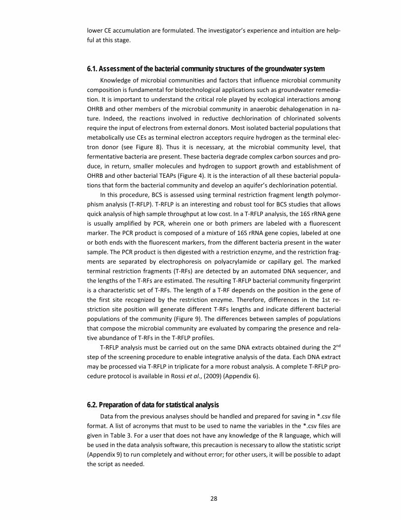
 28 

lower CE accumulation are formulated. The investigator’s experience and intuition are help‐

ful at this stage. 

 

 

6.1. Assessment of the bacterial community structures of the groundwater system

  Knowledge of microbial communities and factors that  influence microbial community 

composition is fundamental for biotechnological applications such as groundwater remedia‐

tion. It is important to understand the critical role played by ecological interactions among 

OHRB and other members of the microbial community  in anaerobic dehalogenation  in na‐

ture.  Indeed,  the  reactions  involved  in  reductive  dechlorination  of  chlorinated  solvents 

require the input of electrons from external donors. Most isolated bacterial populations that 

metabolically use CEs as terminal electron acceptors require hydrogen as the terminal elec‐

tron  donor  (see  Figure  8).  Thus  it  is  necessary,  at  the microbial  community  level,  that 

fermentative bacteria are present. These bacteria degrade complex carbon sources and pro‐

duce,  in  return, smaller molecules and hydrogen  to support growth and establishment of 

OHRB and other bacterial TEAPs (Figure 4). It is the interaction of all these bacterial popula‐

tions that form the bacterial community and develop an aquifer’s dechlorination potential. 

  In this procedure, BCS is assessed using terminal restriction fragment length polymor‐

phism analysis (T‐RFLP). T‐RFLP is an interesting and robust tool for BCS studies that allows 

quick analysis of high sample throughput at low cost. In a T‐RFLP analysis, the 16S rRNA gene 

is usually  amplified by PCR, wherein one or both primers  are  labeled with  a  fluorescent 

marker. The PCR product is composed of a mixture of 16S rRNA gene copies, labeled at one 

or both ends with the fluorescent markers, from the different bacteria present in the water 

sample. The PCR product is then digested with a restriction enzyme, and the restriction frag‐

ments  are  separated  by  electrophoresis  on  polyacrylamide  or  capillary  gel.  The marked 

terminal restriction  fragments  (T‐RFs) are detected by an automated DNA sequencer, and 

the lengths of the T‐RFs are estimated. The resulting T‐RFLP bacterial community fingerprint 

is a characteristic set of T‐RFs. The length of a T‐RF depends on the position in the gene of 

the  first  site  recognized  by  the  restriction  enzyme.  Therefore,  differences  in  the  1st  re‐

striction site position will generate different T‐RFs  lengths and  indicate different bacterial 

populations of the community (Figure 9). The differences between samples of populations 

that compose the microbial community are evaluated by comparing the presence and rela‐

tive abundance of T‐RFs in the T‐RFLP profiles. 

  T‐RFLP analysis must be carried out on the same DNA extracts obtained during the 2nd 

step of the screening procedure to enable integrative analysis of the data. Each DNA extract 

may be processed via T‐RFLP in triplicate for a more robust analysis. A complete T‐RFLP pro‐

cedure protocol is available in Rossi et al., (2009) (Appendix 6). 

 

 

6.2. Preparation of data for statistical analysis

  Data from the previous analyses should be handled and prepared for saving in *.csv file 

format. A list of acronyms that must to be used to name the variables in the *.csv files are 

given in Table 3. For a user that does not have any knowledge of the R language, which will 

be used in the data analysis software, this precaution is necessary to allow the statistic script 

(Appendix 9) to run completely and without error; for other users, it will be possible to adapt 

the script as needed.  

 29 

Other parameters that are not listed in Table 3 can be added to the *.csv file without 

any problems, as long as the data header name does not conflict with the acronyms of the 

listed variables. 

 

 

Figure 9 – Schematic procedure of terminal restriction fragment length polymorphism analysis. It consists of 4 steps: i) PCR amplification of 16S rRNA genes from a complex sample, ii) digestion of the PCR products with a restriction enzyme, iii) electrophoretic separation of the enzymatic products of digestion and iv) recovery of size and abundance data for each separated marked terminal fragment  

 Table 3 – List of the variable names and acronyms to be used in the *.csv files.  

Acronym Teaps variables Acronym CE accumulation Acronym Others variables

PCE perchloroethene X.PCE %PCE Eh redox potential TCE trichloroethene X.TCE %TCE pH acidity c12DCE cis-1,2-DCE X.c12DCE %c12DCE tC temperature (t°C) VC vinyl chloride X.VC %VC eC electric conductivity ethene ethene TOC total organic carbon NO3 nitrate (NO3

-) Cl chloride (Cl-) NO2 nitrite (NO2

-) NH4 ammonium (NH4+) MnII manganese(II) (Mn(II)) FeII iron(II) (Fe(II)) SO4 sulfate (SO4

2-) H2S hydrogen sulfide (H2S) CH4 methane (CH4) CO2 carbon dioxide (CO2) dO2 dissolve oxygen (dO2)

 

 

6.2.1. T-RFLP profiles

  A T‐RFLP profile  from a water sample contains two types of  information:  i) the T‐RFs 

positions in base pairs and ii) the amount of detected fluorescence for each T‐RF (T‐RF peak 

 30 

area  and  height).  These  data  are  extracted  from  the  electropherogram  using  the Gene‐

Mapper  v4.0  software  (ABI).  The  *.txt  output  files  from  the GeneMapper  software  that 

contain T‐RFLP data are opened  in Excel software. Data profiles are aligned semi‐manually 

using Treeflap crosstab macro1 (Rees et al., 2004) by crosstabbing the T‐RFs’ peak area and 

size (rounded to the nearest 1 in setup options). This means that T‐RFs in a profile that differ 

by less than 0.5 bp are considered identical and assigned to the average size. The resulting 

crosstab must be copied and pasted without link in a new Excel sheet to be modified. Peaks 

with an area smaller than 50 relative fluorescence units (RFU) are discarded. T‐RFLP profiles 

that show less than 100,000 RFU in the total of all peak areas are discarded. T‐RFs shorter 

than 50 bp and larger than 500 bp are discarded due to inconsistent results and lack of pre‐

cision in their sizing respectively (max. size of the PCR product is 510 pb). To reduce potential 

biases induced by the inconsistent reproducibility of T‐RFs that show very small amounts of 

fluorescence, T‐RFs less than 300 RFU are suppressed when they are not present in all repli‐

cate profiles of a sample. When all data profiles are treated, the final excel sheet  is saved 

under comma separated value (.csv) format with the name spe.csv (Figure 10). It is important 

to always save T‐RFLP data prepared for statistical analysis under this name, as the file will 

be recalled from the statistical analysis script using this name. 

 

 

 Figure 10 – spe.csv final data matrix in Excel. First column contains name of the samples, first line refers the T-RFs size in base pair (bp). Data corre-spond to the value in RFU of each peak area.  

 

6.2.2. Physicochemical data

  The measured chemical and physicochemical parameters have to be prepared in three 

different *.csv files: teaps.csv, XCEs.csv and others.csv. The teaps.csv file contains CE (includ‐

ing ethene) concentration data and chemical parameters related to TEAPs, i.e. optimally PCE, 

TCE, c12DCE, t12DCE, VC, ethene, NO3‐, NO2

‐, NH4+, Mn(II), Fe(II), SO4

2‐, H2S/S2‐, CH4, CO2, dO2 

(Figure 11).  In addition,  for the  file teaps.csv, all contaminant concentrations must be ex‐

pressed in the same unit (g/L). Percentage of PCE, TCE, DCE and VC can be calculated from 

the sum of contaminant concentrations. These calculated parameters are conserved in a new 

table, XCEs.csv, and will be indicative of accumulation of the different CEs. The others.csv file 

(Figure 13) contains all other measured environmental parameters  (i.e. TOC, ORP/Eh, pH, 

temperature, conductivity, sampling depth, etc.). 

 

 

 31 

   Figure 11 – teaps.csv final concentration matrix in Excel. First column contains name of the samples, first line contains names of CEs and inorganic compounds related to TEAPs. The acronyms used are PCE: perchloroethene, TCE: trichloroethene, c12DCE: cis-1,2-dichloroethene, VC: vinyl chloride, NO3: nitrate, NO2: nitrite, NH4: ammonium, MnII: manganese(II), FeII: iron(II), SO4: sulfate, CH4: methane.  

 

 Figure 12 – XCEs.csv final data matrix in Excel. First column contains name of the samples, first line contains the CE percentages labels.  

 

 Figure 13 – others.csv final data matrix in Excel. First column contains name of the samples, first line contains names of environmental parameters. The acronyms used are Cl: chlorine, F: fluorine, PO4: phosphate, K: potassium, Corg: total organic carbon (TOC), pH: acidity, tC: temperature, turb: turbidity, Eh: oxido/reduction potential, depth: sampling depth.  

 

  The first line of the tables presents names of the measured parameters; avoid concen‐

tration units, dots, and subscript or superscript characters in names (see acronyms listed in 

Table 3). The first column contains the sample names that must be in the same order as in 

the spe.csv file. These names need to be unique, even if the samples come from the same 

sampling well. Then the table is filled with the measured values, where dots, not commas, 

are used as the decimal separator. Optimally the table should not present missing values. It 

 32 

is important that all parameters are documented for each monitoring well; otherwise it will 

be necessary to suppress a whole line or column for the analysis. Measured concentrations 

below the detection limit should be considered as null concentrations and noted as 0 in the 

table. Parameter columns with null values for all samples should be deleted. This information 

should be kept elsewhere as a reminder that the parameter was measured but not detected, 

as may be the case for the ethene concentration parameter. Finally, each excel sheet is saved 

in .csv format under the precise name needed to call it from the statistic script. 

 

 

6.3. Multivariate statistical analysis for integrative analysis of bacterial and environmen-tal data

  The objective for collection of the above bacterial and physicochemical data is to exam‐

ine aquifer ecosystem  functioning as a whole regarding CE dechlorination (section 3). The 

Multiple Factor Analysis (MFA1) was chosen to explore the data and achieve this comprehen‐

sive analysis (Borcard et al., 2011). MFA  is a general type of Principal Component Analysis 

(PCA2).  Its goals are to analyze several data sets of variables collected on the same set of 

observations and to evaluate the relationships between variables or groups of variables (Abdi 

et al., 2013). In our investigation of aquifers, MFA explores data tables in which water sam‐

ples are described by several inter‐correlated quantitative, dependent variables. MFA allows 

the simultaneous exploration of the four data sets of variables: i) the BCS dataset (spe.csv), 

ii) the dataset that indicates the reduction states of the contaminant as well as environmental 

variables related to TEAPs (teaps.csv), iii) the CE accumulation dataset (XCEs.csv), and iv) the 

remaining environmental data  (others.csv). Data  from biomarker detection should not be 

included in MFA since these PCR results, in contrast to the other matrices that present quan‐

titative data,  are qualitative presence/absence data.  Interpretation of  the  resulting MFA 

could be delicate and introduce confusion, and therefore these data should not be used for 

MFA. 

  Each water sample is characterized by its own values of measured parameters. Graph‐

ically, these measurements place the water samples in a multidimensional space defined by 

a number of axes related to the number of measured variables (Figure 14a). The goal of MFA 

is to extract the important information from the whole dataset and represent it in a set of 

new orthogonal axes called MFA dimensions or components (Figure 14b). These new axes 

point to the directions of maximal variance or dispersion of the whole dataset. In MFA, just 

like in standard PCA, the importance of a dimension is reflected by its Eigenvalue percentage, 

which indicates how much of the total variance of the data is explained by this dimension. 

MFA will define as many axes as are needed to describe the total dispersion of samples. Com‐

monly, the first two dimensions are those that describe most of the variance in the data and 

are used for coherent graphical representation  in 2D of the MFA results (Figure 14c). MFA 

also defines the contribution of the former variables in this new MFA space, i.e. the contri‐

bution of the former variables to explain the variance of the data. 

 

 

                                                            

 1 Multiple Factor Analysis in R software: http://factominer.free.fr/advanced‐methods/multiple‐fac‐tor‐analysis.html   2 Principal component analysis explained visually :http://setosa.io/ev/principal‐component‐analysis/  

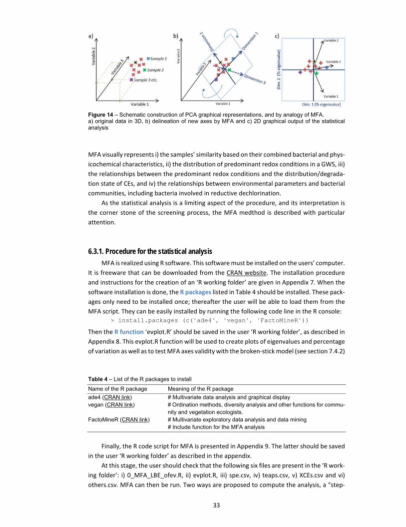
 33 

 Figure 14 – Schematic construction of PCA graphical representations, and by analogy of MFA. a) original data in 3D, b) delineation of new axes by MFA and c) 2D graphical output of the statistical analysis  

 

MFA visually represents i) the samples’ similarity based on their combined bacterial and phys‐

icochemical characteristics, ii) the distribution of predominant redox conditions in a GWS, iii) 

the relationships between the predominant redox conditions and the distribution/degrada‐

tion state of CEs, and iv) the relationships between environmental parameters and bacterial 

communities, including bacteria involved in reductive dechlorination.  

  As the statistical analysis is a limiting aspect of the procedure, and its interpretation is 

the corner stone of the screening process,  the MFA medthod  is described with particular 

attention. 

 

 

6.3.1. Procedure for the statistical analysis

  MFA is realized using R software. This software must be installed on the users’ computer. 

It  is freeware that can be downloaded from the CRAN website. The  installation procedure 

and instructions for the creation of an ‘R working folder’ are given in Appendix 7. When the 

software installation is done, the R packages listed in Table 4 should be installed. These pack‐

ages only need to be installed once; thereafter the user will be able to load them from the 

MFA script. They can be easily installed by running the following code line in the R console:    > install.packages (c('ade4', 'vegan', 'FactoMineR'))  

Then the R function ‘evplot.R’ should be saved in the user ‘R working folder’, as described in 

Appendix 8. This evplot.R function will be used to create plots of eigenvalues and percentage 

of variation as well as to test MFA axes validity with the broken‐stick model (see section 7.4.2) 

 

 Table 4 – List of the R packages to install  

Name of the R package Meaning of the R package

ade4 (CRAN link) # Multivariate data analysis and graphical display vegan (CRAN link) # Ordination methods, diversity analysis and other functions for commu-

nity and vegetation ecologists. FactoMineR (CRAN link) # Multivariate exploratory data analysis and data mining # Include function for the MFA analysis

 

  Finally, the R code script for MFA is presented in Appendix 9. The latter should be saved 

in the user ‘R working folder’ as described in the appendix.  

At this stage, the user should check that the following six files are present in the ‘R work‐

ing  folder’:  i) 0_MFA_LBE_ofev.R,  ii) evplot.R,  iii) spe.csv,  iv) teaps.csv, v) XCEs.csv and vi) 

others.csv. MFA can then be run. Two ways are proposed to compute the analysis, a “step‐

 34 

by‐step way” and an “easy way”. First, the user must verify that the R working directory cor‐

responds  to  the  “R  working  folder”  (Appendix  7),  then  choose  one  of  the  approaches 

described below. 

Step by step way: The user opens the MFA script from the R software and executes line‐by‐

line. The user can read the comments (after each # symbol) placed throughout the script that 

describe the lines of code and guide the user through the script.  

Easy way: If the user is not interested with the details of the analysis, the following line of 

code can be written in the R console to let the script execute alone:  > source("0_MFA_LBE_ofev.R ")  

The MFA output files generated by the script are saved in the ‘R working folder’ under the 

names listed in Table 5. 

 

 Table 5 – List and brief descriptions of the MFA R script output files  

Output file name Brief description

1) 1_Test_Axes.png Show graphically axes validity of the MFA dimensions 2) 2_Plot_CorrelationCircle.png Show correlation between variables and their contribution in the MFA dimensions 1 and 2 3) 3_Plot_CorrelationCircle_0.05.png MFA Correlation circle showing only significant variables (with

a p-value < 0.05) that explain the MFA model 4) 4_Plot_IndFactMap.png Plot of the water samples in the MFA dimensions 1 and 2 5) 5_Table_Correlations_BCS_Env.csv Table of the correlations and associated p-value between the

BCS and groups of environmental variables, and between BCS and variables take separately.

 

 

6.4. Keys for reading MFA plots

  The file ‘1_Test_Axes.png’, which is produced during the MFA, provides a way to evalu‐

ate the statistical validity of MFA axes that describe GWS data. If MFA axes are not validated, 

interpretation of  the results will be wrong.  If validated,  the axes are robust and the MFA 

results are reliable. An example will be detailed in Section 7.4.2. Then the two main, useful 

output plots of the MFA are the ‘Correlation circle’ and the ‘Individual factor map’ (Table 5, 

output files 2, 3 and 4 respectively). A case study of these output plots is presented in Figure 

15 to facilitate comprehension of the reading keys listed below. The case study data imitate 

a contaminated site where no ethene production is detected. 

  Both the ‘Correlation circle’ and ‘Individual factor map’ graphs are composed of a two‐

dimensional plane defined by the two principal dimensions, MFA1 and MFA2. These axes are 

associated with an Eigenvalue percentage that corresponds to the variance among samples 

explained by each axes. For example, in Figure 15, the MFA axes together explain 39.13% of 

the variance between samples, 22.07% along the MFA1 axis and 17.06% along the MFA2 axis.  

  The ‘Correlation circle’ graph (Figure 15) depicts the projection of the original measured 

variables as grey, green, red and blue vectors that correspond respectively to the analyzed 

groups of variables BCS, TEAPs, %CEs and Others (section 6.2). Each parameter is projected 

in the defined MFA two‐dimensional plane according to their respective importance to ex‐

plain the variability of the data. With this graphical output of MFA, all parameters can be 

observed and compared  in a unique referential, the  ‘Correlation circle’ showing the  intra‐ 

and inter‐relationships of the physicochemical and the microbiological parameters.  

 

The keys for reading the ‘Correlation circle’ are: 

 35 

• The longer a vector is, the more the associated variable presents dissimilar values and 

explains the variance among samples. This does not necessarily imply that a long‐length 

vector corresponds to a parameter with high values, but rather to a variable whose val‐

ues are heterogeneous and different  from one sample to another. To appreciate the 

magnitude of the data it is essential to return to raw data. 

• Collinear vectors pointing in the same direction indicate parameters that are positively 

correlated in a GWS (i.e. when a parameter is present at high concentration, the other 

is also at high concentration). For example, this is the case for the NH4+ and TOC vectors 

or the Fe(II) and VC vectors in Figure 15. 

• Vectors pointing in opposite directions from the origin of the graph indicate parameters 

that are negatively correlated in a GWS (i.e. when a parameter is present at elevated 

concentration the other is at low concentration). This is the case for the NO3‐ and NO2

‐ 

vectors or the %PCE and %VC vectors in Figure 15. 

• Perpendicular vectors  indicate parameters  that  are  independent one  from  another. 

This means that no trend links the values of one parameter to the value of the other. 

For example, in Figure 15, the perpendicular position of the tC and Eh vectors indicates 

that temperature is not linked to oxidation‐reduction potential.  

 

 

Figure 15 – Multiple factor analysis (MFA) plots presented as a case study to aid understanding of the reading keys and interpretation of the MFA multivariate statistical analysis. In the ‘Correlation circle’, grey vectors correspond to the projection of the T-RF positions of the T-RFLP profiles (section 6.1) (i.e. interpretable as presence of a bacterial population). Other abbreviations: Eh, oxidation-reduction potential; dO2, dissolved oxygen; X.PCE, percentage of perchloroethene among to-tal CEs; NO3, nitrate; TOC, total organic carbon; NH4, ammonium; VC, vinyl chloride; X.VC, percentage of vinyl chloride among total CEs; FeII, iron(II); tC, temperature, NO2, nitrite. In the ‘Individual factor map’, points n°1 to 20 correspond to the sample projections, which summarize the results obtained from the four variable groups, (BCS, TEAPs, %CEs and Others) for each sample.  

 

  The ‘Individual factor map’ (Figure 15) represents the projection of each sample in the 

MFA dimensions, depicted by gathering the results obtained from the four variable groups, 

BCS, TEAPs, %CEs and Others. This means that the position of a sample on the graph is the 

barycenter of the data of all bacteriological and physicochemical parameters measured for 

this sample. The ‘Individual factor map’ shows the similarity or dissimilarity between water 

 36 

samples according to their relative positions. The keys for reading the ‘Individual factor map’ 

are: 

• The closer  two samples are,  the more similar  they are  in  their physicochemistry and 

microbiology and vice versa. For example, in Figure 15 the close samples 8 and 18 are 

similar, and the distant samples 7 and 10 are dissimilar.  

• Samples close to the center of the MFA graph are few or are not explained by the MFA 

axes. This is the case for samples 4 and 14 in Figure 15. This means that the measured 

parameters  (taken as a whole) are not discriminant  factors and do not elucidate  the 

biogeochemistry of the sample. 

 

  The ‘Correlation circle’ and the ‘Individual factor map’ are different output representa‐

tions of the same MFA and can be read together. This means that: 

The direction indicated by a vector in the ‘Correlation circle’ (Figure 15, left) is associated 

to samples in the same graph area on the ‘Individual factor map’ (Figure 15, right). The 

variable associated with the vector indicates the main discriminant parameter for sam‐

ples in this area of the graph (Figure 15, right). For example, samples 18, 8, 22 and 10 

occupy the area pointed to by the Fe(II), %VC, and VC vectors. This means that water 

samples 18, 8, 22 and 10 are different from the others by the simultaneous presence of 

Fe(II) and vinyl chloride, as well as vinyl chloride accumulation. 

A vector that is collinear to one of the MFA axes indicates that this parameter substan‐

tially  impacts the distribution of the samples along the MFA dimension. For example, 

the collinearity of the dO2 vector with the MFA1 axis indicates that the dissolved O2 con‐

centration is the main factor that explains sample dispersion along the MFA1 axis (i.e. 

samples located in the left part of the graph present higher dissolved O2 concentrations 

than samples in the right part). Similarly, the distribution of the samples along the MFA2 

axis  is explained  in particular by  the vertically positioned NO2‐ and NO3

‐ vectors. The 

sample dispersion along the MFA2 axis is due to differences in NO2‐ and NO3

‐ concentra‐

tions.  

 

 

6.5. Guidelines for MFA interpretation and setting up the GWS biogeochemical model

  The MFA output graph interpretation is the cornerstone for identifying both competi‐

tion  between  bacterial  metabolisms  and  reductive  dechlorination  and  the  reasons  for 

complete or incomplete dechlorination in a GWS.  In this sense, the reading keys presented 

above are the  foundation  for  identifying the  important  factors that affect aquifer biogeo‐

chemical functioning, such as:  

The predominant TEAPs present in a GWS 

Competition  for  electron donors  that occurs between  TEAPs  and CE biodegradation 

(linked to 4.4.1 section and Figure 4) 

The overall connections between measured environmental and microbiological param‐

eters  

 

For example, interpretation of the ‘Correlation circle’ in Figure 15 indicates that 5 predomi‐

nant TEAPs occur in the GWS (for theory help, see Section 4.3.2.2): 

 37 

  (1) The Eh and dO2 vectors on the left part of the ‘Correlation circle’ indicate that the 

presence of oxygen is concomitant with a high oxidation‐reduction potential. These param‐

eters are indicative of the aerobic respiration process. This also means that the right part of 

the graph is probably related to anaerobic bacterial processes. 

  (2) The presence of the NO2‐ vector in the right upper quarter of the ‘Correlation circle’ 

may indicate that the dissimilatory nitrate reduction process (NR) takes place in part of the 

aquifer. In this case, NO3‐ is reduced at least into NO2

‐. The position of the NO2‐ vector in the 

right part of the ‘Correlation circle’ that is related to anaerobic bacterial processes (see point 

1) corroborates this interpretation. However, as mentioned in Section 4.3.2.2., an explana‐

tion for the presence of NO2‐ must be  interpreted with caution and formed  in conjunction 

with other forms of nitrogen. The opposite area of the graph, indicated by the NO3‐ vector, 

signifies that another part of the GWS is characterized by NO3‐ available for denitrification, 

but probably in low concentrations (should be confirmed with raw data), and oxic conditions 

(observed in point (1)) may limit the process. 

  (3) The NH4+ vector  in  the  right  lower part of the graph, collinear  to  the TOC vector, 

indicates that the presence of organic carbon is correlated to NH4+. The bacterial process that 

produces NH4+ under anaerobic conditions (observed in point (1)) and requires large amounts 

of carbon as an energy source is the dissimilatory nitrate reduction to ammonium process 

(DNRA). The origin of NH4+ in the aquifer should nevertheless be taken into consideration to 

avoid misinterpretation. For example, NH4+ could originate from anaerobic degradation (am‐

monification) of organic material or from anthropogenic activities.  

  (4, 5) The VC and %VC vectors are in collinear alignment with the Fe(II) vector. This indi‐

cates that the microbial processes of VC reductive dechlorination and iron(III) reduction are 

in competition with each other and that due to VC accumulation iron(III) reduction inhibits 

VC reductive dechlorination. The iron(III) respiration processes requires similar ranges of re‐

ducing equivalents as DCE reductive dechlorination (electron donor H2, Figure 4). This would 

explain a slowdown of DCE degradation. Second, iron(III) reduction activities require lower 

H2 concentrations than VC reductive dechlorination (Figure 4). This means that  iron(III) re‐

duction wins the competition under low redox conditions, and VC accumulates. 

  Consequently,  the  reason  that  lower CE dechlorination  stalls  in  this example  is  that 

dechlorination of VC to ethene is limited or blocked in the system by iron oxide respiration. 

  Lastly, RV correlation coefficients, which are correlations between the environmental 

and bacterial community datasets, and the associated p‐values, are calculated in MFA; the 

output is located in ‘5_Table_Correlations_BCS_Env.csv’. The RV coefficients can reveal sig‐

nificant  correlations  between  bacterial  communities/populations  with  ongoing 

biogeochemical processes or identify a microbiological lack. An example of these results will 

be detailed in the next section of this document, which describes a concrete application of 

the screening procedure through a complete case study. 

 

 38 

 

7. CASE STUDIES  

APPLICATION OF THE SCREENING PROCEDURE FOR THE EVALUATION OF THE NATURAL 

ATTENUATION POTENTIAL IN CE‐CONTAMINATED AQUIFERS  

 

7.1. Case study 1 - Former dry-cleaning facility, Canton of Solothurn, Switzerland

 

This first case study was detailed in Shani et al., (2013). The complete document can be 

downloaded  from  the website of  the  journal Environmental Science and Technology  (doi: 

10.1021/es304017s). A short summary of this site  investigation  is provided here. The site 

(Figure 16) was a former dry‐cleaning facility operated from the mid‐1940s until 1987. A ma‐

jor subsurface PCE contamination event occurred in 1969. 

 

 

 Figure 16 - Map of the Solothurn test-site. Monitoring wells are shown as colored circles (left). The source of the PCE contamination is shown as a star. The general groundwater flow direction is indicated with a blue arrow. The circle colors indicate the local oxidation–reduction status at the monitoring location. Green: oxic/nitrate-reducing, orange: nitrate to iron-reducing, red: iron-reducing and brown: methanogenic. Concentrations of CEs measured from two sampling campaigns (A: April and B: October 2008 respectively) are shown on the left. The figure is extracted from the Shani et al., 2013 publication.  

 

VC accumulated in situ overall, as shown previously with stable isotope techniques (Aep‐

pli  et  al.,  2010), while  complete  reductive  dechlorination  and  the  corresponding  ethene 

production occurred locally. Shani et al. (2013) followed a procedure similar to the present 

protocol to investigate the reasons for this. 

 

 39 

The procedure involved the 3 steps: i) collection of the aquifer’s biogeochemical data, 

ii) confirmation of biochemical potential through the CE reductive dechlorination process via 

PCR detection of both RdhA and OHRB 16S rRNA genes and via microcosm studies, iii) eluci‐

dation of the mechanisms responsible  for  incomplete  in situ dechlorination of CEs via the 

correlations between BCS and the environmental variables (TEAPs and Others) determined 

by MFA. In order to validate the mechanisms proposed in the third and last step of the pro‐

tocol,  this  study  additionally  presents  a  deeper  bacterial  analysis,  which  identifies  the 

bacterial populations associated with the terminal restriction fragments (T‐RFs) that signifi‐

cantly correlated with TEAP variables. 

The MFA showed that TEAPs shaped the structure of the bacterial community (BCS) in 

general. VC and iron(III) reduction were both keys and antagonistic microbiological processes 

in  this  aquifer. An  interpretation of  this  result  could be  that  the  iron‐reducing bacteria’s 

higher affinity for hydrogen, as compared to VC‐reducing bacteria (Figure 4), would explain 

the inefficient complete dechlorination and the local VC accumulation. The detailed molecu‐

lar analyses of BCS showed that the bacterial populations that correlated significantly with 

VC reduction were those affiliated to the genus Dehalococcoides and to the “Lahn Cluster” 

(included  in  the  class  Dehalococcoidetes).  Conversely,  T‐RFs  affiliated  with  the  genus 

Rhodoferax, known to harbor iron‐reducing bacterial species, were anti‐correlated to “Lahn 

Cluster” T‐RFs. These results supported the hypothesis that competition between reductive 

dechlorination and iron‐reduction was the bacterial‐dependent mechanism that limited the 

natural attenuation of VC in the aquifer.   

In conclusion, this first integrative environmental and microbial data analysis is a helpful 

example that identifies the reasons for accumulation of toxic dechlorination intermediates. 

 

 

7.2. Case study 2 - Former municipal discharge site, Canton of Geneva, Switzerland

 

7.2.1. Site information

  This case study was carried out on a PCE‐contaminated site near Geneva, Switzerland, 

and the monitoring and study was entrusted to BG Consulting Engineers (BG). The site is cur‐

rently occupied by family gardens and was originally a municipal landfill (probably a place of 

wild repository). The site map is presented in Figure 16, where the main investigation area is 

surrounded with green lines (around 13000 m2). At the time of the investigation, the site was 

equipped with 24 monitoring wells, two of which could be sampled at two different depths 

(MIP05 and MIP06). 

  The soil profile analysis of a NNW‐SSE transect (Figure 17) indicated that the groundwa‐

ter  system  is  composed  of  upper  and  lower  aquifers  with  different  groundwater  flow 

directions (Figure 18a and b). They are separated by a horizon of compacted sandy  loamy 

gravel with low permeability, but fractures in some parts of the horizon allow water to flow 

from the upper to the lower aquifer.  

 

 

 

 40 

 Figure 17 – Map of the studied site contaminated with chlorinated ethenes and distribution of the moni-toring wells.  

 

Figure 18 – Soil profile of a NNW-SSE transect of the studied site contaminated with chlorinated ethenes, and projection of the piezometer positions on the transect plane. Blue lines indicate the limits of the upper and lower aquifers.  

7.2.2. Assessing in situ presence of reductive dechlorination – Step 1

  Twenty‐five water samples were collected from 24 piezometers (MIP01, MIP02, MIP03, 

MIP04, MIP05‐upper, MIP05‐lower, MIP06‐lower, MIP07, MIP08, MIP10, MIP11, MIP20, 

PO1, PO2, PO3, PO4, PO5, PO6, PO7, PO8, PO10, PO11, S12099, S12512, S20), and the phys‐

icochemical  parameters  listed  in  section  3  of  the  procedure  were  analyzed.  The 

physicochemical data is given in Appendix 10A. The contaminant maps presented in Figures 

19 and 20 were produced based on the results of CE concentration measurements. 

 

 

 

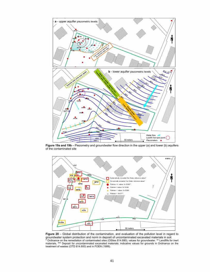
 41 

Figure 19a and 19b – Piezometry and groundwater flow direction in the upper (a) and lower (b) aquifers of the contaminated site  

 Figure 20 – Global distribution of the contamination, and evaluation of the pollution level in regard to groundwater system protection and norm in deposit of uncontaminated excavated materials in soil. * Ordinance on the remediation of contaminated sites (OSites 814.680), values for groundwater. ** Landfills for inert materials, *** Deposit for uncontaminated excavated materials: indicative values for grounds in Ordinance on the treatment of wastes (OTD 814.600) and in FOEN (1999).

   

b - lower aquifer piezometric levels

a - upper aquifer piezometric levels

 42 

  On this site, PCE, c12DCE and VC concentrations were above legal limits. PCE was dechlo‐

rinated  until  c12DCE  and  VC  along  the  groundwater  flow  direction.  This  created  a 

contaminant plume, from the NNW to SSE axis, where c12DCE and VC concentrations were 

10‐ and 50‐fold higher than legislation limits, respectively (Figure 20). No ethene production 

was detected at the site. Hence, the reductive dechlorination process occurred at the site, 

but is incomplete. 

 

 

7.2.3. Evaluation of the biochemical potential for reductive dechlorination - Step 2

 

7.2.3.1. Detection of biomarkers

  A total of 25 water samples were analyzed for the biomarkers for OHRB and RdhA genes 

listed in 4.2.3. The results are summarized in Figure 21 and detailed in Table 6. All biomarkers 

were detected at the site (Table 6), and at least one of the biomarkers was detected per well. 

The  two most commonly detected genera of OHRB were Desulfitobacterium and Desulfu‐

romonas, from which strains are known to dechlorinate PCE to c12DCE (Figure 7‐C and Figure 

8). One or both of these genera were found alone, without detection of other OHRB or RdhA 

genes,  in 52% of the samples. This was the case for the wells PO10 and MIP20; where the 

highest c12DCE concentration was reported and only one OHRB was detected (Desulfitobac‐

terium or Desulfuromonas, Table 6). These results  indicate that part of the site  lacked the 

bacterial guild required for complete dechlorination. 

 

 Figure 21 – Map of the contaminants PCE, TCE, c12DCE and VC produced at the site. CE concentrations are plotted as circles with a size proportional to their concentration values. Red circles correspond to concentrations that exceed the OSites limits (shown in the red box). Black circles corre-spond to non-zero concentrations below OSites limits. The scale used to plot the VC concentration is 100 fold higher than the one used for the other CEs.  

  Conversely, the genus Dehalococcoides, from which there are strains known to dechlo‐

rinate CEs to ethene, was detected in 4 samples, and the bvcA and vcrA genes, which code 

for VC dehalogenase catalytic  subunits, were detected  in 6  samples. Detections occurred 

close to the contamination source and equally  in the upper and  lower aquifers. However, 

 43 

only dechlorination to VC was observed in these wells, and both VC and c12DCE concentra‐

tions were  high.  Hence,  the  detection  of  Dehalococcoides  sp.  and  RdhA  genes without 

concomitant ethene production suggests that environmental conditions were inadequate for 

reductive dechlorination of c12DCE and VC or that the species detected did not possess the 

complete dechlorination functionality. 

 

 Figure 22– Map of biomarkers detected at the site. The size of the circle is proportional to the number of markers identified at each well. The yellow circle distinguishes the two sampling depths (1 upper, 2 lower) of well MIP05. No water sample could be re-trieved from MIP06-1.  

  In conclusion, the reductive dechlorination biomarker assessment showed that OHRB 

and RdhA genes were present in some wells and demonstrated that the actors and biochem‐

ical potential for complete dechlorination of PCE to ethene was present in this aquifer.  It was 

difficult to know if the observed incomplete dechlorination was due to adverse environmen‐

tal conditions or an incorrect assessment of the biological function. Microcosm experiments 

can clarify which cause limited PCE degradation. 

 

7.2.3.2. Microcosm experiments

Sediments were sampled from soil cores from newly drilled wells: PO7, PO8, PO10, and PO11. 

Samples were taken from the saturated zones of the cores. Microcosms experiments were 

prepared as described  in Appendix 5, except that  instead of water, 15‐20 mL of sediment 

were taken as inoculum. Microcosms were cultivated for 4 months at 37°C. 1 mL of electron 

donor solution (MixII, Appendix 5) was added in each microcosm every three weeks after GC 

analysis of the microcosm gas composition. After 73 days of cultivation, all microcosms re‐

duced PCE to c12DCE. Only sample PO7‐(8.10) was able to reduce PCE to VC. Microcosms 

were followed for 130 days, and the last measurements are presented in Table 7. After 122 

days, 4 of 7 microcosms developed the ability to reduce PCE to VC, and after 130 days, two 

microcosms, PO8 and PO10, started to produce ethene. Figure 23 shows the microcosms at 

the end of the experiment. 

 

 Table 6 – Presence (+) / absence (-) of biomarkers assessed by specific PCR on DNA extracted from aquifer water samples.

 44 

-1 and -2 refer to upper and lower aquifer samples, respectively, of wells MIP05 and MIP06.

 

 Table 7 – Dechlorination products detected in the gas phase of microcosms after 122 and 130 days of incubation. Sample names are followed by the sampling depth in meters in parentheses.  

Time Sample PCE TCE DCE CV ethene

122 days PO7-(7.20) X X X PO7-(8.10) X X X X PO8-(6.20) X X X X PO8-(7.10) X X X X PO10-(7.50) X X X PO10-(9.30) X X X X PO11-(8.70) X X X 130 days PO7-(7.20) X X X PO7-(8.10) X X X X PO8-(6.20) X X X X X PO8-(7.10) X X X X PO10-(7.50) X X X PO10-(9.30) X X X X PO11-(8.70) X X X

 

 Figure 23 – The organohalide-respiring bacteria (OHRB) enrichment culture microcosms from aquifer sediments after 130 days.

Wel

l na

me

Deh

aloc

occ

oid

es

sp.

Deh

alob

acte

r sp

.

Sul

furo

spir

ilium

sp.

Des

ulfu

rom

ona

s sp

.

Des

ulfi

toba

cter

ium

sp.

Ge

oba

cte

r sp

.

bvc

A

vcr

A

MIP01 - - - + + - - - MIP02 + - + + + - - - MIP03 - - - + + + - - MIP04 - - - + - - + - MIP05-1 + + - - + - - - MIP05-2 + + - + + + + + MIP06-2 - - - + + - - - MIP07 - - - + + + - - MIP08 - - - + - - - - MIP10 - - - + + + - - MIP11 - - - + + - - + MIP20 - - - - + - - - PO1 - - - + + - - + PO2 - - - + + - - - PO3 - - - - + - - - PO4 - - - + - - - - PO5 - - - + - - - - PO6 + - + + + - - + PO7 - - - + + - + + PO8 - + - + + - - - PO10 - - - + - - - - PO11 - - - + - - - - S12099 - - - + - - - - S12512 - - - + + - - - S20 - - - + - - - -

 45 

  Because PCR detection was conducted with water samples and the microcosm experi‐

ments were conducted with sediments, the results of these two methods cannot be directly 

compared. Nevertheless,  the main conclusion was  that  in optimal conditions,  the studied 

GWS expressed the biochemical potential for complete dechlorination of PCE to ethene. 

 

 

7.2.4. Biogeochemistry of the aquifer: elucidate the reason for the observed incomplete reductive dechlorination of PCE – Step 3

 

7.2.4.1. Bacterial community structure investigation

  T‐RFLP analysis was realized on 23 DNA extracts from the groundwater (the same DNA 

as the biomarker detection). Data were handled as described in the procedure, and raw T‐RF 

data, including number, position and detected intensity per T‐RFLP profile, are presented in 

Appendix 10B. Samples MIP05‐1 and PO11 were excluded as they gave T‐RFLP profiles whose 

total intensities were less than 100,000 RFU. PO7 was also excluded as this sample came from 

a well identified after the sampling campaign as outside of the main aquifer (Figure 17).  

 

7.2.4.2. Statistical analysis of the entire data set

  The data were submitted to statistical analysis as presented in the procedure. The mean‐

ing of MFA  is to compare samples defined by different groups of variables. Recall that the 

data sets are structured in different groups:  i) “BCS”, which corresponds to the T‐RFs of the 

BCS described in each sample by T‐RFLP analysis (spe.csv, Appendix 10B); ii) “TEAPs”, which 

corresponds to water chemistry analysis results related to TEAPs (teaps.csv, Appendix 10A); 

iii) “%CEs”, which corresponds to CE accumulation (XCEs.csv, Appendix 10A); and iv) “Oth‐

ers”, which corresponds to environmental parameters not related to TEAPs, such as pH, Eh, 

etc. (others.csv, Appendix 10A). 

 

  The first figure obtained relates to the MFA axes validity analysis (Figure 24). MFA axes 

were sorted  in descending order by their Eigenvalues, which represent the portion of the 

total variance explained by the sample variance. According to Borcard et al. (2011), there are 

two ways to evaluate which axes are important and representative for visualization of data: 

i) the Kaiser‐Guttman criterion (KGC), which calculates the mean of all eigenvalues and indi‐

cates interpretable axes that present eigenvalues larger than this mean (Figure 24, left) or ii) 

the Broken stick model (BSM), which presents random eigenvalues (Figure 24, right, red), and 

compares them to eigenvalues extracted from the MFA model. MFA axes with eigenvalues 

larger than those generated by BSM can be interpreted. BSM is more restrictive than KGC, so 

it is more robust and is recommended for this analysis. If only one axis is validated, then data 

interpretation will only be correct along this axis. The two first axes are always those with 

the highest Eigenvalues,  i.e. those that will best represent the variance between samples. 

Calculation of eigenvalue percentages quantifies the proportion of the variance explained by 

each MFA axis (axis percentages), and the percentage sum for the two first axes gives the 

proportion of variance shown by the graphical representation of the MFA model (Figures 24 

and 10). 

 

 

 46 

 Figure 24 – Representation of Kaiser – Guttman criterion (left) and Broken-stick model (right) tests of MFA axes. Output file: 1_MFA_AxesValidity.png  

 

 Figure 25 – Correlation circle, graphical output file: 2_MFA_CorrelationCircle.png  

 

  Figure 25 is the second graph that was generated by the MFA analysis and corresponds 

to file “2_MFA_CorrelationCircle.png”. This MFA representation is difficult to read since the 

numerous  grey  vectors  related  to  the  T‐RFs  of  the  BCS  group  partially  hide  the  other 

variables. This MFA graph shows that the bacterial population vectors (X50 to X500) point in 

all directions of the correlation circle, and some are close to some environmental vectors. 

The links between the BCS and environmental parameters will be discussed in 7.2.4.3. 

  Figure 26 is the 3rd graph that was generated by the MFA analysis and corresponds to 

the file “3_MFA_CorrelationCircle_0.05.png”. It provides a suitable and  legible representa‐

tion of the results. This correlation circle shows only the variables that significantly (p < 0.05) 

contribute to one or both MFA axes. These variables are most likely to explain the variance 

between samples in the first two dimensions of the MFA, i.e. are the most important physi‐

cochemical and bacterial parameters that drove the aquifer redox conditions at the sampling 

time. This MFA representation focuses on the predominant variable links that are essential 

 47 

to explore in order to evaluate the potential for natural CE dechlorination in a contaminated 

aquifer.  

  The correlation circle and the individual factor map (Figure 27), where samples are plot‐

ted instead of the variable vectors, can be read at the same time. Each sample has a point of 

coordinates in each group of variables, and the individual factor map plots the barycenter of 

a sample (Figure 27, black dots) based on its coordinates in each group of variables. 

 

7.2.4.3. Interpretation of the statistical analysis output plots

  The objective during MFA interpretation is to establish a model of the predominant re‐

dox conditions in the aquifer in relation to the CE degradation state and the support provided 

by the bacterial community structures. Interpretation is based on the bacterial and physico‐

chemical characterizations, and during  interpretation, the studied GWS  is considered as a 

whole (Figure 2). 

  MFA interpretations were done using the guidelines provided in the procedure (section 

5.4.). Altogether, the MFA dimensions explained 32.8% of the variance. The sample distribu‐

tion along axis 1 of  the MFA was mainly characterized by  the variables: TCE and c12DCE 

concentrations; TCE and c12DCE percentages; and Mn(II), NH4+ and TOC concentrations. The 

sample distribution along axis 2 was mainly characterized by NO2‐ and Eh, and the BCS varia‐

bles are mostly correlated with axis 2. 

  The MFA model indicates that there were different local geochemical conditions in the 

studied GWS. The Eh and dO2 vectors (Figure 26) indicate that samples in the lower left quar‐

ter of the MFA  (Figure 26) were characterized by higher redox potential and dissolved O2 

values than the other samples. The redox potential values of the aquifer ranged between ‐

107.6 mV to 286.5 mV (Appendix 10A), where 9 out of 10 samples registered above 0 mV. 

70% of the samples had a dissolved O2 concentration higher than 0.5 mg/L. This means that, 

globally, the aquifer was under slightly reducing conditions, though locally, aerobic/aero‐tol‐

erant or anaerobic bacterial processes were possible. 

  The NO2‐ vector, along axis 2 (Figure 26) and in opposite part of the Eh vector, indicates 

that samples  in the upper part of the MFA  (Figure 27) were  locally characterized by NO3‐

reducing conditions (NO3‐‐> NO2

‐). NO2‐concentrations reached as high as 3940 µg/L (Appen‐

dix 10). 

  The NH4+ vector, which belongs to axis 1 on the right (Figure 26), suggests that in other 

areas of the aquifer, where NH4+ concentrations were as high as 4000 µg/L (Appendix 10), 

dissimilatory nitrate reduction to ammonium (DNRA) could have taken place. DNRA was doc‐

umented  in anoxic marine sediments  (Tiedje, 1998) and  is possible  in GWSs  (Smith at al., 

1991), but normally plays a minor role since NH4+ is stable only in reduced conditions. In the 

specific context of the studied site, NH4+ could also have come from organic mineralization 

in the upper part of the soil in the landfill area, as is indicated by the concomitant presence 

of the TOC vector. The NO3‐concentration was high in many samples (> 5mg/L, Appendix 10), 

and only when this concentration was lower were the NH4+ or NO2

‐ concentrations often high. 

This corroborates the interpretation that nitrate‐reducing conditions were present. 

 

 

 48 

 Figure 26 – Correlation circle, graphical output file: 3_MFA_CorrelationCircle_0.05.png. Grey vectors correspond to the projection of the T-RF positions of the T-RFLP profiles. Eh, oxidation-reduction potential; dO2, dissolved oxygen; X.PCE / X.TCE / X.cDCE, percentage of perchloroethene / trichloroethene / cis-1,2-dichloroethene respectively among total CEs; NO2, nitrite; TOC, total organic carbon; NH4, ammonium; PO4, phosphate; x, position of well along north-south axis; F, Fluoride; pH, ; CH4, methane; MnII, manganese(II); depth, depth of the water sampling; c12DCE, cis-1,2-dichloroe-thene ; K, potassium ion.  

 

 Figure 27 – Individual map factor, graphical output file: 4_MFA_IndFactMap.png.  

 

 49 

  The CH4 vector (Figure 25) indicates that in some samples its presence is discriminant, 

however it  is  important to note that the CH4 concentration was low at the site (< 50 µg/L, 

Appendix 10). Its origin could be microbial or the landfill itself. If microbial, CH4 would have 

originated from methanogenic archaea, but only in localized microsites as the general redox 

potential (Eh min. ‐10 mV) was not reduced enough for methanogenesis. 

  Concomitant presence of the Mn(II), TCE, %TCE, c12DCE and %c12DCE vectors gives the 

most important information regarding the dechlorination activity in the GWS. The spatial dis‐

tribution of these vectors provides the key for the  interpretation of the main mechanisms 

that occurred  in the aquifer. The simultaneous occurrence of the Mn(II), TCE and c12DCE 

vectors indicates that samples plotted in the right part of the MFA (Figure 26) were under 

manganese‐reducing  and  reductive  dehalogenation  conditions.  Figure  4  (section  3.4.1) 

shows that these two processes require the same amount of reducing equivalents to occur. 

At this site, manganese reduction was in competition with TCE and c12DCE degradation. Con‐

sequently, the kinetics of the reductive dechlorination process was locally disturbed by the 

reduction of manganese oxides, and  the weak VC and undetected ethene concentrations 

(Appendix 10) at the site were a consequence of this reductive dechlorination inhibition. TCE 

accumulated locally, however the TCE concentration never exceeded the limit set by OSites. 

This indicates a slight negative difference between the supply and the degradation rates of 

the TCE pool. However, this  is much more marked  for the c12DCE pool, which was highly 

accumulated at the site (Figure 20). 

 

7.2.4.4. Analysis of relationships between environmental variables and BCS

  The relationships between the environmental variables and the BCSs were explored in 

this case study in order to highlight the processes predominantly sustained by the microbiol‐

ogy. For this, RV correlation coefficients (RV coeff.) were calculated from the MFA model. 

The RV correlation coefficient indicates the closeness of the two sets of values, and the asso‐

ciated p‐value indicates the robustness of the correlation. Table 8 presents the RV correlation 

coefficient calculated between the BCS and the other groups of variables (TEAPs, %CEs and 

Others), and between  the BCS and each environmental parameter  individually. To under‐

stand the meaning of a correlation between the BCS and a parameter, it is necessary to keep 

in mind that the number of different types of bacteria and their relative abundance in a sam‐

ple defines the structure of a bacterial community. This measure of the relationship between 

the BCS matrix and one environmental parameter is used to show schematically that when a 

chemical concentration changes from one sample to another, the global structure of the bac‐

terial community also changes, and vice versa.  

  Table 8 shows that only the group of variables “Others” was significantly correlated with 

the BCS matrix. Among the variables of this group, the parameter Eh was the only one signif‐

icantly linked to the BCS matrix. This result shows, as expected, that microbial communities 

clearly affected the global redox potential of the GWS and vice versa.  

  The groups TEAPs and %CEs were not globally correlated with BCS. In these groups, only 

the variables %TCE, NO2‐, and CH4 presented significant correlations with BCS. The robust RV 

correlation coefficient confirms that CH4 concentrations, although  low, were  linked to bio‐

logical activity. As the CH4 concentration is low and the redox potential is high at the site, CH4 

should be consumed by methane‐utilizing bacteria  (methanotrophs, Hanson and Hanson, 

1997) even though it is produced locally by methanogens in saturated microsites in the soil. 

The significant connection between the BCS and NO2‐ concentration indicates that the bac‐

terial  communities  supported  nitrate  reduction  in  the  GWS  area  of  concern.  Nitrate 

reduction engages specialized microorganisms as obligate respiratory bacteria that belong to 

 50 

genera such as Agrobacterium, Alcaligenes, Bacillus, Paracoccus denitrificans, Pseudomonas 

and Thiobacillus.  

 Table 8 – RV correlation coefficients and the associated p-values calculated between the bacterial com-munity dataset and i) each defined group of environmental variables (TEAPs, %CEs, Others) and ii) each environmental variable separately.

Variables RV coeff. p-value Significance TEAPs 0.3756 0.2087 ns %CEs 0.3190 0.0601 ns Others 0.4830 0.0056 **

PCE 0.1245 0.8006 ns TCE 0.1042 0.9141 ns c12DCE 0.0970 0.9519 ns VC 0.2021 0.0954 ns NH4

+ 0.1271 0.7045 ns NO3

- 0.1435 0.5977 ns NO2

- 0.2587 0.0074 **

SO42‐ 0.1306 0.6713 ns

Fe(II) 0.1447 0.5134 ns Mn(II) 0.1449 0.5227 ns CH4 0.3046 0.0085 ** dO2 0.2331 0.0598 ns %PCE 0.1666 0.3198 ns %TCE 0.2454 0.0325 * %c12DCE 0.1784 0.2483 ns %VC 0.2054 0.0506 ns Eh 0.3051 0.0099 ** pH 0.2207 0.0713 ns t°C 0.1802 0.2439 ns TOC 0.1382 0.5748 ns Chloride 0.1694 0.3200 ns

Degree of significance based on the calculated p-value: **, significant p-value < 0.01; *, moderately significant p-value < 0.05; ns, non-significant. RV coeff. : RV correlation coefficient. This table is generated from the output files: 5_MFA_Correlations_BCS _gp-var.csv.

 

 

  Mn(II), TCE and c12DCE, which highlighted within the interpretation of the ‘Correlation 

circle’, were not significantly correlated with the BCS matrix. Different microorganisms can 

reduce Mn(IV) and Fe(III);  for example, the genera Bacillus, Geobacter, and Pseudomonas 

harbor manganese‐reducing bacteria (Lovley, 2006). However, these bacteria have a versa‐

tile metabolism and are not dedicated to the manganese reduction process.  In fluctuating 

conditions, these bacteria are able to adapt their respiratory metabolism and use alternative 

terminal electron acceptors. These bacterial populations are non‐discriminants for manga‐

nese reduction which translates into unspecific correlations with the manganese reduction 

process. The same observations can be made about the bacteria implicated in the first steps 

of the reductive dechlorination process  (e.g. Sulfurospirillum, Desulfitobacterium, Desulfu‐

romonas, Figure 8, versatile metabolisms). These statements should elucidate why the Mn(II) 

and CE vectors were not yet directly associated to a characteristic BCS, even if the  oxidation‐

reduction  potential was within  the  range where manganese(IV)  reduction  predominates 

(around 200 mV). Then, when the aquifer reaches a stable, specific redox condition over a 

long period of time, specialized and obligate e.g. manganese‐reducing bacteria (Myers and 

Nealson, 1988) could emerge in the BCS.  

 

 

 

 51 

7.2.5. Conclusions - Scenarios for incomplete in situ reductive dechlorination

  The first step of the procedure, the analysis of the contaminant distribution and their 

degradation state, has shown that reductive dechlorination was present at the site, but that 

the  process was  incomplete.  The  second  step,  screening  for  the  presence  of  OHRB  bi‐

omarkers and their biochemical potential, has indicated that the GWS contains the genetic 

markers as well as  the  functional capacity  to perform complete dechlorination. The  third 

step, the analysis of the GWS biogeochemical state, has deepened the understanding of the 

aquifer functioning at the time of the inventory. The main identifiable explanation for incom‐

plete  dechlorination  is  that  the  local  redox  conditions  at  the  site were  not  sufficiently 

reducing. The presence of non‐negligible concentrations of electron acceptors other than CEs 

mobilized the reducing power (H2) to the detriment of reductive dechlorination. Manganese 

reduction  interfered  locally  by  slowing  the  reductive  dechlorination  of  TCE  and  c12DCE. 

Therefore, until manganese oxides are completely reduced, dechlorination of c12DCE will be 

inhibited or at least occur at a low rate.  

  Based on the results of the procedure, it is most improbable that complete natural at‐

tenuation of PCE will occur  in a  reasonable timeframe.  It  is probable  that the system will 

naturally  tend  towards global accumulation of c12DCE and  local accumulation of VC. The 

presence of specific biomarkers linked to the last stage of PCE dechlorination (vcrA and bvcA), 

and the evidence of ethene production obtained in microcosms, indicates that under favor‐

able  conditions  complete  removal  could  be  achieved  globally.  CEs  may  be  completely 

eliminated if the redox conditions are modified in the aquifer by adding a suitable substrate 

(electron donor). Hence, enhanced natural attenuation (ENA) is a conceivable remediation 

strategy. 

 

   

 52 

 

REFERENCES  

Abdi, H., and Williams, L.J. (2010) Principal component analysis, Wiley Interdisciplinary Reviews: Computational Statistics, Vol. 2(4): 433–459 - doi: 10.1002/wics.101

Abdi, H., Williams, L., and Valentin, D. (2013). Multiple factor analysis: principal component analysis for multitable and multiblock data sets.WIREs Comp. Stat. 5, 149–179.

ADEME (2007) Natural attenuation of chlorinated aliphatic compounds in aquifers - Methodological Guide - ADEME Collection “Know to Act” - R&D program MACAOH (Modeling, Attenuation, Characterization in Aquifers of OrganoHalogens), Côme J.M., Ropars M., Kaskassian, S., Quintard M., Vogel T., Razakarisoa O., Nex F., Schäfer G., Haeseler F., 230 pp. (available in French) http://www.ademe.fr

Aeppli, C., Hofstetter, T. B., Amaral, H. I. F., Kipfer, R., Schwarzenbach, R. P., Berg, M.(2010) Quantifying in situ transformation rates of chlorinated ethenes by combining compound-specific stable isotope analysis, groundwater dating, and carbon isotope mass balances. Environmental Science and Technology. 44, 3705– 3711

Behrens, S., Azizian, M.F., McMurdie, P.J., Sabalowsky, A., Dolan, M.E., Semprini, L., and Spormann, A.M. (2008) Monitoring abundance and expression of “Dehalococcoides” species chloroethene-reductive dehalogenases in a tetrachloroethene-dechlorinating flow column. Applied and Environmental Microbiology. 74 (18), 5695–5703.

Böhlke, J.K., Smith, R.L., Miller, D.N. (2006) Ammonium transport and reaction in contaminated groundwater: Application of isotope tracers and isotope fractionation studies. Water Resources Research. 42. http://dx.doi.org/10.1029/2005WR004349

Bond, D.R., Holmes, D.E., Tender, L.M., and Lovley, D.R. (2002) Electrode-reducing microorganisms that harvest energy from marine sediments. Science. 295 (5554), 483–485.

Borcard, D., Gillet, F., and Legendre, P. (2011) Numerical Ecology with R, Springer. ISBN 978-1-4419-7975-9 (Print) 978-1-4419-7976-6 (Online).

Bradley, P.M. (2003) History and Ecology of Chloroethene Biodegradation: A Review. Bioremediation Journal. 7(2): 81-109, doi:10.1080/ 713607980

Chapelle, F.H., McMahon, P.B., Dubrovsky, N.M., Fujii, R.F., Oaksford, E.T., and Vroblesky, D.A. (1995) Deducing the distribution of terminal electron-accepting processes in hydrologically diverse groundwater systems. Water Resources Research. 31: 359-371.

Chapelle, F., Widdowson, M.A., Brauner, J.S., and Mendez, E. (2003). Methodology for estimating times of remediation associated with monitored natural attenuation. U.S. Geological Survey Water-Resources Investigation Report 03-4057. 51 pages. http://pubs.usgs.gov/wri/wri034057/.

Chloronet (2009) Guide of Chlorinated hydrocarbons (HCC): Properties and behavior in the environment. FOEN. 50p. (available in French and German) http://www.bafu.admin.ch/chloronet/06273/index.html?lang=fr

Dowideit, K., Scholz-Muramatsu, H., Miethling-Graff, R., Vigelahn, L., Freygang, M., Dohrmann, A.B. and Tebbe, C.C. (2010) Spatial heterogeneity of dechlorinating bacteria and limiting factors for in situ trichloroethene dechlorination revealed by analyses of sediment cores from a polluted field site. FEMS microbiology ecology. 71, 444-59.

Duhamel M. and Edwards E.A. (2006) Microbial composition of chlorinated ethene-degrading cultures dominated by Dehalococcoides. FEMS Microbiology Ecology. 58(3): 538-549.

Ebersole R. and Hendrickson E. (2003) Nucleic acid fragments for the identification of dechloprinating bacteria. Patent WO/2003/064, 695.

EPA (2008) Sampling guidance for unknown contaminants in drinking water. EPA-817-R-08-003, 71pp., http://nepis.epa.gov/Exe/ZyPURL.cgi?Dockey=P1002CNX.txt

 53 

EPA (2000) Engineered Approaches to In situ Bioremediation of Chlorinated Solvents: Fundamentals and Field Applications. EPA 542-R-00-008, 144pp. http://nepis.epa.gov/Exe/ZyPURL.cgi?Dockey=10002UIJ.txt

EPA (1999) Microbial Processes Affecting Monitored Natural Attenuation of Contaminants in the Subsurface. EPA/540/S-99/001, 18pp. http://nepis.epa.gov/Exe/ZyPDF.cgi/10002E30.PDF?Dockey=10002E30.PDF 

EPA (1998) Technical Protocol for Evaluating Natural Attenuation of Chlorinated Solvents in Ground Water. EPA/600/R-98/128, 248 pp. http://nepis.epa.gov/Exe/ZyPDF.cgi/30003ONO.PDF?Dockey=30003ONO.PDF 

Federal Council (2015) Environment Switzerland 2015, Report of the Federal Council, Bern, series: State of the environment. n° er2015, 144pp. . (available in English, French, German and Italian) http://www.bafu.admin.ch/publikationen/publikation/01794/index.html?lang=en  

Federal Environment Agency (Umweltbundesamt) (2011) Consideration of natural attenuation in remediating contaminated sites, 42pp. http://www.umweltbundesamt.de/en/publikationen/consideration-of-natural-attenuation-in-remediating

FOEN (2013) Analytical methods in the field of waste and polluted sites. Series: Environment in practice. n° UV-1334-F, 80 pp. (available in French and German) http://www.bafu.admin.ch/publikationen/publikation/01752/index.html?lang=fr  

FOEN (2000) Contaminated sites, endangering evaluation - Specifications for the technical investigation of contaminated sites. Series: Environment in practice. n° VU-3406-F, 25pp. (available in French and German) http://www.bafu.admin.ch/publikationen/publikation/00499/index.html?lang=fr

FOEN (2003) Sampling of groundwater in relation to contaminated sites. Series: Environment in practice. n° VU-3413-F, 28pp. (available in French and German) http://www.bafu.admin.ch/publikationen/publikation/00505/index.html?lang=fr

FOEN (2001a) Contaminated sites: register, evaluate, remediate. Series: Non-specialist publications. n° DIV-3400-E: 49pp. (available in French, German, Italian and English) http://www.bafu.admin.ch/publikationen/publikation/00495/index.html?lang=en

FOEN (2001b) Development of remediation projects of contaminated sites. Series: Environment in practice. n° VU-3410-F: 36pp. (available in French, and German) http://www.bafu.admin.ch/publikationen/publikation/00502/index.html?lang=fr

FOEN (2004) Practical guidelines for the protection of groundwater. Series: Environment in practice. n° VU-2508-F, 133p. (available French, German and Italian ) http://www.bafu.admin.ch/publikationen/publikation/00378/index.html?lang=fr

FOEN (1994) Management concept of contaminated sites for Switzerland. Objectives and measures Series: Environmental notebook. n°220, SRU-220-F , 34pp. (available in French)

FOEN (1999) Directive for valorization, treatment and storage of excavation materials and spoil (Directive on excavation materials). VU-3003-F, 20 pp.

Futagami, T., Goto, M., and Furukawa, K. (2008) Biochemical and genetic bases of dehalorespiration. Chemical Record. 8, 1-12.

Futagami, T., Goto, M., and Furukawa, K. (2014) Chapter 4, Genetic System of Organohalide-Respiring Bacteria. In H. Nojiri et al. (eds.), Biodegradative Bacteria: How Bacteria Degrade, Survive, Adapt, and Evolve. doi:10.1007/978-4-431-54520-0_4

Garcia-Cantizano, J., Casamayor, E.O., Gasol, J.M., Guerrero, R., Pedros-Alio, C. (2005) Partitioning of CO2 incorporation among planktonic microbial guilds and estimation of in situ specific growth rates. Microbial Ecology. 50: 230–241. doi: 10.1007/s00248-004-0144-9

Grandel, S., and Dahmke, A. (2008) Leitfaden – Natürliche Schadstoffminderung bei LCKW-kontaminier- ten Standorten. KORA Themenverbund 3: Chemische Industrie, Metallverarbeitung. Institut für Geo- wissenschaften, CAU Kiel, ISBN 978-3-00-026094-0.

 54 

Goldscheider, N., Hunkeler, D., Rossi, P. (2006) Review: Microbial biocenoses in pristine aquifers and an assessment of investigative methods. Hydrogeology Journal. 14(6), 926-941.

Hiraishi, A. (2008) Biodiversity of dehalorespiring bacteria with special emphasis on polychlorinated biphenyl/dioxin dechlorinators. Microbes and Environments. 23: 1-12.

Hendrickson, E.R., Payne, J.A., Young, R.M., Starr, M.G., Perry, M.P., Fahnestock, S., Ellis, D.E., and Ebersole, R.C. (2002) Molecular analysis of Dehalococcoides 16S ribosomal DNA from chloroethene-contaminated sites throughout north America and Europe. Applied and Environmental Microbiology. 68(2), 485-495.

Holliger, C., Schraa, G., Stams, A.J.M., and Zehnder, A.J.B. (1992) Enrichment and properties of an anaerobic mixed culture reductively dechlorinating 1,2,3-trichlorobenzene to 1,3-dichlorobenzene. Applied and Environmental Microbiology. 58, 1636-1644.

Holliger, C., Schraa, G., Stams, A.J.M., and Zehnder, A.J.B. (1993) A highly purified enrichment culture couples the reductive dechlorination of tetrachloroethene to growth. Applied and Environmental Microbiology. 59, 2991-2997.

Humphreys, W.F. (2006). Aquifers: the ultimate groundwater-dependent ecosystems. Australian Journal of Botany. 54, 115-132.

Kampbell, D.H., Wilson, J.T., Vandegrift, S.A. (1989) Dissolved oxygen and methane in water by a GC heaspace equilibrium technique. International Journal of Environmental Analytical Chemistry. 36, 249-257.

Lane D.J. (1991) 16S/23S rRNA sequencing In: Nucleic Acid Techniques in Bacterial Systematics (Stackebrandt, E. and Goodfellow, M., Eds.), pp. 115–175. Wiley, Chichester, UK.

Lanthier, M., Villemur, R., Lepine, F., Bisaillon, J.G. and Beaudet, R. (2001) Geographic distribution of Desulfitobacterium frappieri PCP-1 and Desulfitobacterium spp. in soils from the province of Quebec, Canada. FEMS Microbiology Ecology. 36 (2-3), 185–191.

Lindenbaum J. (2012) Identification of sources of ammonium in groundwater using stable nitrogen and boron isotopes in Nam Du, Hanoi. Dissertations in Geology at Lund University, No. 300, 38 pp.

Lorah, M., and Voytek, M. (2004) Degradation of 1,1,2,2-tetrachloroethane and accumulation of vinyl chloride in wetland sediment microcosms and in situ porewater: biogeochemical controls and associations with microbial communities. Journal of Contaminant Hydrology. 70, 117-145.

Lovley, D. (2006) Dissimilatory Fe(III)- and Mn(IV)-Reducing Prokaryotes. The Prokaryotes, CHAPTER 1.21, 2:635–658, doi:10.1007/0-387-30742-7_21

Major, D., McMaster, M., Cox, E., Edwards, E., Dworatzek, S., Hendrickson, E., Starr, M., Payne, J. and Buonamici, L. (2002) Field Demonstration of Successful Bioaugmentation to Achieve Dechlorination of Tetrachloroethene to Ethene. Environmental Science Technology. 36, 5106-5116.

Maphosa, F., de Vos, W., and Smidt, H. (2010) Exploiting the ecogenomics toolbox for environmental diagnostics of organohalide-respiring bacteria. Trends in biotechnology. 28, 308–16.

McMahon, P., and Chapelle, F. (2008) Redox processes and water quality of selected principal aquifer systems. Ground water. 46, 259–71.

Middeldorp, P., Luijten, M., Pas, B., Eekert, M., Kengen, S., Schraa, G. and Stams, A. (1999) Anaerobic Microbial Reductive Dehalogenation of Chlorinated Ethenes. Bioremediation Journal. 3, 151-169.

Myers, CR., and Nealson, KH. (1988) Bacterial Manganese Reduction and Growth with Manganese Oxide as the Sole Electron Acceptor. Science, Vol. 240: 1319-1321. doi:10.1126/science.240.4857.1319

Palumbi, S.R., Martin, A., Romano, S., McMillan, W.O., Stice, L. and Grabowski, G. (2002). The Simple Fool's Guide to PCR, Version 2.0. Privately published, Univ. Hawaii. http://palumbi.stanford.edu/SimpleFoolsMaster.pdf

 55 

Parsons Corporation. (2004) Principles and Practices of Enhanced Anaerobic Bioremediation of Chlorinated Solvents. For AFCEE, NFESC, ESTCP, USACE. 022/738863/28.doc. http://costperformance.org/remediation/pdf/principles_and_practices_bioremediation.pdf

Rees, G., Baldwi,n D., Watson, G., Perryman, S. and Nielsen, D. (2004) Ordination and significance testing of microbial community composition derived from terminal restriction fragment length polymorphisms: application of multivariate statistics. Antonie Van Leeuwenhoek, 86(4): 339-347. doi: 10.1007/s10482-004-0498-x.

Rossi, P., Gillet, F., Rohrbach, E., Diaby, N., Holliger, C. (2009) Statistical assessment of the variability of the T-RFLP analysis applied to complex microbial communities. Applied and Environmental Microbiology. 75, 7268–7270. doi:10.1128/AEM.00135-09 http://aem.asm.org/content/early/2009/09/11/AEM.00135-09.full.pdf+html

Rousk, J., and Bengtson, P. (2014) Microbial regulation of global biogeochemical cycles. Frontiers in Microbiology, 5. http://dx.doi.org/10.3389/fmicb.2014.00103

Shani, N. (2012) Assessing the Bacterial Ecology of Organohalide Respiration for the Design of Bioremediation Strategies, EPFL thesis n° 5379, doi:10.5075/epfl-thesis-5379

Shani, N., Rossi P. & Holliger C. (2013) Correlations between environmental variables and bacterial community structures suggest Fe (III) and vinyl chloride reduction as antagonistic terminal electron-accepting processes. Environmental science & technology 47, 6836–6845. doi:10.1021/es304017s

Smits, T.H., Devenoges, C., Szynalski, K., Maillard, J. and Holliger, C. (2004) Development of a real-time PCR method for quantification of the three genera Dehalobacter, Dehalococcoides, and Desulfitobacterium in microbial communities. Journal of Microbiological Methods. 57(3), 369–378.

Smith, R.L., Howes, B.L., Duff, J.H. (1991) Denitrification in nitrate-contaminated groundwater: occurrence in steep vertical geochemical gradients. Geochimica et Cosmochimica Acta. 55, 1815–1825.

Tiedje, J.M. (1988) Ecology of denitrification and dissimilatory nitrate reduction to ammonium. p. 179-244. In A.J.B. Zehnder (ed), Environmental Microbiology of Anaerobes. John Wiley and Sons, N.Y.

Tiehm, A., and Schmidt, K.R. (2011). Sequential anaerobic/aerobic biodegradation of chloroethenes-aspects of field application. Current Opinion in Biotechnology. 22, 415–421. doi:10.1016/j.copbio.2011.02.003

Tobiszewski, M., and Namieśnik, J. (2012) Abiotic degradation of chlorinated ethanes and ethenes in water. Environmental Science and Pollution Research. 19, 1994–2006.

Treseder, K., Balser, T., Bradford, M., Brodie, E., Dubinsky, E., Eviner, V., Hofmockel, K., Lennon, J., Levine, U., MacGrego,r B., Pett-Ridge, J., Waldrop, M. (2011) Integrating microbial ecology into ecosystem models: challenges and priorities. Biogeochemistry. 109, 7–18.

Turner, S., Pryer, K.M., Miao, V.P.W., and Palmer, J.D. (1999) Investigating deep phylogenetic relationships among cyanobacteria and plastids by small subunit rRNA sequence analysis. Journal of Eukaryotic Microbiology. 46, 327–338.

Weissbrodt, D.G., Shani, N., Sinclair, L., Lefebvre, G., Rossi, P., Maillard, J., Rougemont, J., Holliger, C. (2012) PyroTRF-ID: a novel bioinformatics methodology for the affiliation of terminal-restriction fragments using 16S rRNA gene pyrosequencing data. BMC Microbiology. 12, 306. doi:10.1186/1471-2180-12-306

 

   

 56 

APPENDIX 1 

   GROUNDWATER QUALITY  

Indicative values for groundwater quality presented in appendix A1 of ”Practical guidelines 

for the protection of groundwater “ (FOEN, 2004) and modified from appendix 2 of the “Fed‐

eral Ordinance on the Remediation of Polluted Sites, OSites 814.201”. 

 

 

  

 

 

 

 

 

 

 

Paramètres physiques

Température écart d’au moins 3 °C par rapport à l’état naturel

Turbidité <1 UT/F

pH écart d’au moins 0,5 par rapport à l’état naturel

Constituants principaux et secondaires

Calcium (Ca2+) 40 mg/l de plus qu’à l’état naturel

Magnésium (Mg2+) 10 mg/l de plus qu’à l’état naturel

Sulfates (SO42+) <40 mg/l (1)

Silice dissoute (H4SiO4) 10 mg/l de plus qu’à l’état naturel

Baryum (Ba2+) 0,5 mg/l de plus qu’à l’état naturel

Sodium (Na+) 25 mg/l de plus qu’à l’état naturel

Potassium (K+) 5 mg/l de plus qu’à l’état naturel

Chlorures (Cl-) <40 mg/l (1)

Fluorures (F-) 0,5 mg/l de plus qu’à l’état naturel

Bromures (Br-) 0,05 mg/l de plus qu’à l’état naturel

Nitrates (NO3-) <25 mg/l (1)

Ammonium (NH4+)

<0,1 mg/l (1) dans des conditions oxydantes

<0,5 mg/l (1) dans des conditions anoxiques

Nitrites (NO2-) 0,05 mg/l de plus qu’à l’état naturel

Phosphates (o-PO43-) 0,05 mg/l de P de plus qu’à l’état naturel

Cyanures (CN-) <0,025 mg/l

Saturation en oxygène (O2)

>20%

Fer (Fe) dissous 0,3 mg/l de plus qu’à l’état naturel

Manganèse (Mn) dissous 0,05 mg/l de plus qu’à l’état naturel

Carbone organique dis-sous (DOC)

<2 mg/l (1)

1 Valeurs figurant en annexe 2, ch. 22, Œaux.

 57 

 

  

   

Eléments en traces

Bore (B ) <0,05 mg/l de plus qu’à l’état naturel

Zinc (Zn ) dissous <5 µg/l

Cuivre (Cu ) dissous <2 µg/l

Nickel (Ni ) dissous <5 µg/l

Plomb (Pb ) dissous <1 µg/l

Cadmium (Cd ) dissous <0,05 µg/l

Mercure (Hg ) dissous <0,01 µg/l

Arsenic (As ) <5 µg/l

Sélénium (Se ) <5 µg/l

Chrome (Cr ) <2 µg/l

Substances organiques naturelles et de synthèse

Composés organiques halogé-nés adsorbables (AOX)

<10 µg/l (1)

AOX, y compris HHV <10 µg/l

Phénols volatils (entraînables à la vapeur)

<5 µg/l

Hydrocarbures aromatiques monocycliques (BTEX)

<1µg/l pour chaque substance (1)

Hydrocarbures aliphatiques <1 µg/l pour chaque substance (1)

Hydrocarbures halogénés volatils (HHV)

<1 µg/l pour chaque substance (1)

Chlorure de vinyle <0,1 µg/l

Pesticides <0,1 µg/l pour chaque substance (1), somme <0,5 µg/l

Composés nitro-aromatiques totaux

<0,5 µg/l

EDTA et complexants de struc-ture analogue

<5 µg/l pour chaque substance

NTA <3 µg/l

Hydrocarbures aromatiques polycycliques (HAP)

<0,1 µg/l pour chaque substance (1)

Benzo(a)pyrène <0,01 µg/l

Méthyl-tert-butyléther (MTBE) <2 µg/l

Chlorophénols absence d’odeur

Pentachlorophénol <0,1 µg/l

Chlorobenzène <1 µg/l pour chaque substance

Di(2-éthylhexyl)-phtalate (DEHP) <1 µg/l

Amines aromatiques <0,1 µg/l pour chaque substance, somme <0,5 µg/l

Triazoles benzéniques <1 µg/l pour chaque substance

Acides halogénés <0,5 µg/l pour chaque substance

1 Valeurs figurant en annexe 2, ch. 22, Œaux.

 58 

APPENDIX 2 

  CHLORINATED ETHENES ANALYSES   

 

Extract from FOEN (2013) Analytical methods in the field of waste and polluted sites. Series: 

Environment in practice. n° UV‐1334‐F, 80 pp 

 

 

 

   

 59 

APPENDIX 3 

   DNA EXTRACTION PROTOCOL  

 

DNA isolation from filters using Maxwell 16 Instrument (Promega) 

 

Materials:  Maxwell 16 Tissue DNA purification Kit (Promega, Cat.#. AS1030) 

  Maxwell 16 Instrument (Promega, Cat.# AS2000) configured with the Maxwell 16 SEV Hardware 

  Kit (Promega, Cat.# AS1200) 

 

Materials and additional solutions to be supplied by the user: 

n‐butanol p.a.  CAS n° CAS n° 71‐36‐3 

SDS 10% (w/v)  Dodecyl Sodium Sulfate (SDS) ‐ CAS n°151‐21‐3        Prepared solutions using ultrapure water       (e.g. from Direct‐Q® 8 Ultrapure Water System, Merck Millipore)       Do not sterilized       Stock at room temperature to avoid crystallization 

Phosphate Buffer  Mix 94.7% of Na2HPO4 0.12M ‐ CAS n° 7558‐79‐4        0.12M, pH8  with 5.3% NaH2PO4 0.12M ‐ CAS n° 7558‐80‐7     Prepared solutions using ultrapure water     Sterilized the solutions by autoclaving 15’ at 120°C     Stock at 4°C (max. 6 months) 

Proteinase K solution  Specific activity 2.5U/mg (Macherey‐Nagel, ref. 740506)     Adjust concentration regarding specific activity if using another provider 

1.5mL sterilized storage microtubes for final purified DNA samples   (e.g. Eppendorf Safe‐Lock Tubes™, ref. 0030 123.328) 

50mL “Falcon” tubes  ensured for n‐butanol and centrifugation resistance, this last is also link with the    centrifuge model (e.g. Starstedt tubes, ref. 62.547.254) 

Automated pipettes (e.g. Socorex, Acura® manual 825 adjustable volume micropipettes,) 

Sterilized cottoned tips  (e.g. Promega, Promega Barrier Tips) 

Sterilized tweezers  

 

Protocol: 1.  Place 2 filters from a same sample in a 50 mL “Falcon” tube(under a laminar flow  

    hood)  

  2.  Add 10mL of Phosphate Buffer and 1mL of SDS 10% (under a laminar flow hood) 

  3.  Mix and incubate at 70°C for 30min. 

  4.  Add 50µl of proteinase K solution (under a laminar flow hood) 

  5.  Mix and incubate at 65°C for 30min. 

  6.  Remove the filter from the falcon tube (under a laminar flow hood) 

  7.  Mix the remain 11mL of sample solution with 40mL of n‐butanol and vortex (under a 

    fume hood) 

  8.  Centrifuge at 5000rpm, 5min. at RT 

  9.  Remove upper n‐butanol phase, there still remain n‐butanol (under a fume hood) 

 

  The next steps take place with the Maxwell 16 Instrument by using the Maxwell 16 Tissue 

  DNA purification Kit (refer for details to the Promega protocol for users)  

 60 

  10.  Place Cartridges into the cartridge preparation rack, one for each sample and max. 16 

  per purification run. 

  11.  Transfer 400µl of the remaining aqueous phase obtained in step 9 into the 1st well of 

    the cartridge  

  12.  Add 250 µL of elution buffer (provide in the Promega kit) into the blue Elution Tube 

    (provide in the kit), one for each prepared Cartridges. 

  13.  Unsure that the Maxwell16 robot is in SEV RSRC mode, and program the Maxwell 16 

    instrument   by selecting   RUN, DNA, Tissue (see also point 7.B of Promega protocol 

    for usage details) 

  14.  Transfer Cartridges containing samples and plungers from the preparation rack onto 

    the Maxwell 16 platform 

  15.  Place a blue Elution Tube for each cartridge into the Elution Tube Slots at the front of 

    the platform 

  16.  Press RUN/STOP, the platform will retract and the instrument will begin the  

    purification run (running time ~45 min) 

 

   

 61 

APPENDIX 4 

   PCR PROTOCOL  

 

 

 

 

‐ All PCR reagents are provided by PeqLab Biotechnologie GmbH (Germany) provide all PCR 

reagents for this protocol, except if mentioned differently in the text.  

‐ Amplification reactions are carried out in a Thermal Cycler T3  Biometra  (Biolabo  Scientific  

Instruments,  Switzerland) or peqSTAR 96 Universal gradient (Peqlab Biotechnologie GmbH, 

Germany) .  

 

The 16S rRNA genes of OHRB are amplified in a nested PCR procedure. In the first step, 16S 

rRNA  gene  pools  are  amplified  in  30  µl  reaction  mixtures  (Table  A)  using  Eub28f  (5’‐

GAGTTTGATCNTGGCTCAG‐3’)  /  Univ1492r  (5’‐GGYTACCTTGTTACGACTT‐3’)  primers.  PCR 

products of the first PCR are diluted prior to be used for the second amplification step. In the 

second amplification step,  taxon‐specific primers  (Table 2, main document) were used  to 

amplify the 16S rRNA gene of known OHRB in 10 µl reaction mixtures (Table B). 

 

Table A ‐ 1st PCR reaction 

dNTPs : is a generic term referring to the four deoxyribonucleotide triphosphates: dATP, dCTP, dGTP and dTTP. These are 

the building blocks of DNA. 

 

PCR cycle program for the first PCR reaction 1. 94°C for 5’    initial denaturation 2. 30 cycles of   94°C for 30’’   denaturation     50°C for 45’’   annealing     72°C for 1’   elongation 3. 72°C for 10’    final elongation 4. 4°C forever    storage  

 

 

PCR components  Initial concentration  Final concentration  for 30 l reaction  final volume 

Ultrapure type1 sterilized water 

‐  qsp. final reaction volume 

14.10 l 

Buffer  S 

with MgCl2 include 

10X 15mM 

1X 1.5mM 

3.00 l 

dNTPs  10mM each  800M  0.60 l Enhancer P  5X 1X 6.00 l Eub28f  10M  0.5M  1.50 l Univ1492r  10M  0.5M  1.50 l Taq polymerase peqGOLD 

5U/L  add 1/100 of the final reaction volume 

0.30 l 

DNA extract  2ng/L  add 1/10 of the finalreaction volume 

3.00 l 

 62 

Table B ‐ 2nd PCR reaction 

 

PCR cycle program for the second PCR reaction 1.  94°C for 5’    initial denaturation 2.  30 cycles of   94°C for 30’’   denaturation     55°C for 45’’   annealing     72°C for 45’’   elongation 3.  72°C for 10’    final elongation 4.  4°C forever    storage  

 

The VC reductase genes vcrA and bvcA (GenBank YP003330719 and AY563562) are amplified 

in 10 µl reaction mixtures (Table C).  

 

Table C – Reaction mixture for PCR amplification of vcrA and bvcA genes 

 PCR cycle program for vcrA and bvA direct amplification 1.  94°C for 4’30’’    initial denaturation 2.  40 cycles of   94°C for 30’’   denaturation     55°C for 45’’   annealing     72°C for 30’’   elongation 3.  72°C for 10’    final elongation 4.  4°C forever    storage  

PCR components  Initial  concentra‐tion 

Final concentration for 10 l reaction  final volume 

Ultrapure type1 sterilized water 

‐  qsp. final reaction volume  4.10 l 

Buffer  Y 

with MgCl2 include 

10X 20mM 

1X 2.0mM 

1.00 l 

dNTPs  10mM each 3.2mM 0.80 l Enhancer P  5X  1X  2.00 l Primer 1  10M  0.5M  0.50 l Primer 2  10M  0.5M  0.50 l Taq polymerase peqGOLD 

5U/L  add 1/100 of the final reaction volume 

0.10 l 

DNA extract  2ng/L  add 1/10 of the final reaction volume 

1.00 l 

PCR components  Initial  concentra‐tion 

Final concentration  for 10 l reaction  final volume 

Ultrapure type1 sterilized water 

‐  qsp. final reaction volume  3.60 l 

Buffer  S 

with MgCl2 include 

10X 20mM 

1X 1.5mM 

1.00 l 

dNTPs  10mM each  1.2mM  0.30 l Enhancer P  5X  1X  2.00 l Primer 1  10M  1M  1.00 l Primer 2  10M  1M  1.00 l Taq polymerase peqGOLD 

5U/L  add 1/100 of the finalreaction volume 

0.10 l 

DNA extract  2ng/L  add 1/10 of the final reaction volume 

1.00 l 

 63 

 After amplification reaction, the PCR products were checked for size in comparison to 100bp 

ladder (Promega) on 1.5% agarose gels stained with GelRed (Stratec Molecular, Germany) 

after electrophoresis (5Volt/cm during 60’) in TEA 1X and U.V. photographed using a transil‐

luminator device.   The expected sizes for the different resulting PCR products are  listed  in 

Table D.  

 

            

Presence of a PCR product at the right size on the gel indicates presence of the corresponding 

organism in the sample, and can be record as a positive result. Inversely, absence of a PCR 

signal indicates that the targeted organism is absence/lower than the detection limit of the 

PCR methodology, and can be record as a negative result. All presence/absence PCR results 

are finally grouped in a table for further analysis. 

 

 

   

PCR product for  Expected size

Bacteria  1480 pb Dehalococcoides sp.  627 pbDehalobacter sp.  227 pb Sulfurospirillum sp.  634 pb Desulfuromonas sp.  556 pb Desulfitobacterium sp. 213 pbGeobacter lovleyi  412 pbvcrA  139 pb bvcA  247 pb 

 64 

APPENDIX 5 

ENRICHMENT CULTURE  

 

Medium for anaerobic enrichment cultures of aquifer water samples 

Enrichment of reductive dechlorinating bacteria/OHRB as other anaerobic microorganisms, need oxy‐

gen‐free conditions during cultivation. The main things that you have to keep in mind are: 

Make all the solutions in anaerobic water 

Work in a “sterile” space e.g. around a Bunsen burner 

Put overpressure in the head space of your cultures, flushing with N2 and/or CO2  

Materials 

 

N2, CO2, H2 gas station 

Hand crimper (Sigma‐Aldrich, product # 22316‐U) 

100mL Serum Bottles (Sigma‐Aldrich, product #33110‐U) 

20mm Aluminum crimp seals (Sigma‐Aldrich, product #27230‐U) 

Septum stopper in material compatible with chlorinated solvents (e.g. in Butyl, Bellco, #2048‐11800, in Viton) 

Syringes (Terumo, 2‐part syringes 20 mL #SS+T20ES1, 10 mL #SS+T10ES1, 5mL # SS+T05ES1, 2 mL #SS+T02S1)  

Needles (Terumo, brown #NN‐2623R, blue #NN‐2325R, Orange #NN‐2516R) 

Sterile 0.22 µm pore size filters preconditioned in filtration system for syringe (Sarstedt, Filtropur S 0.22 µm, #83.1826.001) 

 Anaerobic medium preparation 

 

In a 100 mL serum bottles pressurize closed with N2 gas to 0.5 bar overpressure (15 cycles of gas ex‐changes i.e. vacuum/gas injection) and autoclaved (20’ at 121°C), sterilely add:  45 mL  Solution A (inorganic phosphates + redox indicator + organic nitrogen and carbon) 1.25 mL  Solution B (vitamins + trace elements) 2.50 mL  Solution C (carbonates + reducing agent solution) 1.25 mL  Solution D (Ca and Mg) Exchange gas of the bottle using around 15 cycles of vacuum / 80%N2:20%CO2 gas injection  Add 5 mL  PCE (100 mM) prepared in Hexadecane (electron acceptor) Add 1 mL  MixII (substrate, electron donors) Add 5 mL  aquifer water as inoculum  

Inoculum must be inject in culture medium without contact with PCE in Hexadecane 

1 mL of MixII should be add every week or two weeks  

Solution A 

 

Solution A contains in final concentration:  Example for 1 liter of Solution A: 

4.2 mM  K2HPO4 * 3H2O  0.958g   K2HPO4*3H2O 

1.4 mM   NaH2PO4 * 2H2O  0.218g  NaH2PO4*2H2O 

0.5 mg.L‐1  Resazurin (from a Resazurin at 0.5 g.L‐1)   0.1g  Peptone 

 65 

0.1 g.L‐1   Peptone  1 mL  Resazurin solution (0.5 g.L‐1) 

    Adjust volume to 1 liter with Mili‐Q water 

 

Prepare the Solution A in a 2L Herlen‐Meyer 

Boil during 20’‐30’ the solution to degas, then cool to room temperature with bubbling  of 80%N2:20%CO2 gas in the solution 

Distribute 45mL of Solution A in the 100 mL serum bottles 

Seal the bottles with stoppers (Butyl) and crimp seals  

Change atmosphere in the bottle with 15 cycles of gas exchange with 80%N2:20%CO2 and finish with 0.5 bar overpressure in the bottles. 

Autoclave 15 min at 121°C 

Conservation 9 ±1 months at room temperature, in the dark. If the initial blue‐purple color turns to pink the solution is passed and should be discarded 

The 0.5 g.L‐1 Resazurin (7‐Hydroxy‐3H‐phenoxazin‐3‐one 10‐oxide) is a blue dye solution (oxygen indicator), should be stock at 4°C, exp. 2 years ±2 months 

 Solution B 

 

In a serum bottle containing 20mL anaerobe Milli‐Q water, add through a 0.2µm sterile filter: 1 ml of Trace element solution ‐ Solution IV 1 ml of Vitamin solution – Solution V 1 ml of Vitamin B1 solution – Solution VI   1 ml of Vitamin B2 solution – Solution VII    1 ml of Vitamin B12 solution – Solution VIII  Anaerobe Milli‐Q water: 

Boil during 20’‐30’ Milli‐Q water and then cool to room temperature with bubbling of N2 

Dispense 20 mL of the water in 100mL serum bottles 

Seal the bottles with the stoppers (Butyl or Viton) and crimp seals  

Change atmosphere in the bottle with 15 cycles of gas exchange with N2 and finish with 0.5 bar overpressure in the bottles 

Autoclave 20’ at 121°C 

Keep anaerobe Milli‐Q water at RT (exp.  1 year ± 1month)  Trace element solution ‐ Solution IV  

Solution IV contains in final concentration:  Example for 1 liter of Solution IV: 

1.711 mM   EDTA   500 mg/l   EDTA   10.06 mM  FeCl2*4H2O  2000 mg/l  FeCl2*4H2O   505.3 µM   MnCl2*4H2O  100 mg/l  MnCl2*4H2O 798.5 µM  CoCl2*6H2O  190 mg/l  CoCl2*6H2O 513.5 µM   ZnCl2  70 mg/l  ZnCl2 15 µM   CuCl2*2H2O  2.6 mg/l  CuCl2*2H2O 41 µM   AlCl3  5.5 mg/l  AlCl3 97 µM   H3BO3  6 mg/l  H3BO3 171 µM   Na2MoO4*2H2O  41.4 mg/l  Na2MoO4*2H2O 101 µM  NiCl2*6H2O  24 mg/l  NiCl2*6H2O   Add 1 liter Mili‐Q water  •  In a 1L Becher dissolve EDTA in a volume of Milli‐Q water equivalent to 3/4 of the final volume.  •  Dissolve Iron(II) Chloride HCl, then add to the EDTA solution. •  Calibrate a pH meter between 4 and 7, and adjust EDTA solution to pH 7 with concentrated HCl. •  Add trace elements, by dissolving them one by one •  Make up to the desire final volume with Milli‐Q water 

 

 66 

Vitamin solution – Solution V 

Solution V contains in final concentration:   Example for 1 liter of Solution V:  

0.20 µM  Biotin (vitamin H)(p‐aminobenzoic)  50 mg        1.57 µM  P‐aminobenzoate (Na‐salt)   250 mg   0.21 µM   Pantothenate (Na‐salt)    50 mg       0.04 µM   Folic acid (dihydrate)    20 mg         0.24 µM  Lipoic acid (thioctic acid)    50 mg       0.59 µM   Pyridoxine (B6 vitamin)    100 mg     4.50 µM   Nicotinamide  550 mg         Dissolve in 1 L Milli‐Q water Vitamin B1 solution – Solution VI 

100mg/l   Thiamine HCl  (Hydrochloride)           Dissolve in Milli‐Q water  Vitamin B2 solution ‐ Solution VII  

50mg/l  Riboflavine (B2 vitamine)       Dissolve in Milli‐Q water          Vitamin B12 solution ‐ Solution VIII  

50mg/l  Cyanocobalamin (vitamin B12)         Dissolve in Milli‐Q water            For Solution V, VI, VII and VIII: 

Prepared 4X100 mL serum bottles pressurize closed with N2 gas to 0.5 bar overpressure (15 cycles of gas exchanges to remove normal atmosphere) and autoclaved (15’ at 121°C). 

Filtrate 50 mL of solution through a 0.22 µm filter in serum bottle (one bottle for each solution). 

Cover each bottle with an aluminum sheet to avoid photolysis 

Stock at 4°C (exp. 2 years ± 1 month)  

Solution C  

 

To 49 mL of solution IX, add 1 mL of solution X  

Conservation: strictly 10 days at 4°C 

Solution C is pink at the beginning then turn transparent as redox decrease with Na2S  Solution IX : 

Solution IX contains in final concentration:   Example for 1 liter of Solution IX:  

110mM  NH4HCO3  9.01 g      0.9 M  NaHCO3  76.11 g         Dissolve in 1 L Milli‐Q water    

Boil the solution to dissolve the powder and then cool to room temperature with bubbling of N2 

Dispense 49 mL in 100mL serum bottles 

Seal the bottles with stoppers (in Butyl or Viton) and crimp seals  

Change atmosphere in the bottle with 15 cycles of gas exchange with 80%N2:20%CO2 and finish with 0.5 bar overpressure in the bottles. 

Autoclave 15’ at 121°C 

Conservation 12 ±1 months at room temperature, in the dark      Solution X : 

Dissolve 24.02 g of washed Na2S*9H2O in 100 mL of Milli‐Q water, and flush with N2 

Prepared empty 100 mL serum bottles pressurize closed with N2 gas to 0.5 bar overpressure and autoclaved. 

 67 

Assemble a syringe, a 0.22 µm syringe filter and a needle 

Filtrate sterilely the solution with in the serum bottle 

Conservation: 6 ±1 months at 4°C  

Solution D 

 

Solution C contains in final concentration:  Example for 1 liter of Solution C: 

30mM CaCl2*2H2O     4.4g de de CaCl2*2H2O  20mM MgCl2*6H2O     4.06g de MgCl2*6H2O   Add 1000 mL Milli‐Q water  

Dispense 200 mL in 500 mL serum bottles 

Seal the bottles with the stoppers (Butyl or Viton) and crimp seals  

Change atmosphere in the bottle with 15 cycles of gas exchange with N2 and finish with 0.5 bar overpressure in the bottles 

Autoclave 20’ at 121°C 

Keep at room temperature (exp. 2 years ± 1month)  

Substrate preparation – electron donors Mix II 

 

Prepared empty 100 mL serum bottles pressurize closed with N2 gas to 0.5 bar overpressure and autoclaved (15’ at 121°C) 

Mix equal volume (1:1:1) of:   Ethanol 100mM     Propionate 100mM     Butyrate 100mM 

Filtrate sterilely the mix with an assembled syringe/0.22 µm filter/needle in the serum bottle 

Keep at 4°C (exp. 1 years ± 1month)  

Ethanol 100mM:  Propionate 100mM:  Butyrate 100mM: 606.20µl absolute ethanol  917.85µl n‐butyric acid  746.82µl Propionic acid Add 100 mL Milli‐Q water  Add 100ml Milli‐Q water  Add 100 mL Milli‐Q water   For each solution: 

Dispense in 100 mL serum bottle 

Seal the bottles with the stoppers (Butyl or Vitton) and crimp seals  

Change atmosphere in the bottle with 15 cycles of gas exchange with N2 and finish with 0.5 bar overpressure in the bottles 

Autoclave 121°C, 20min           

Keep at 4°C, exp. 1 year ± 1 month  

PCE solution – electron acceptors 

 

Tetrachloroethene/Perchloroethene (PCE) Molecular weight PCE 165.834 g/mol ‐ Density PCE 1.623 g/ml ‐ 1L pure PCE is 9.787 mol/L  •  Add 98.98 mL Hexadecane to a 200 mL serum bottle •  Close with a Viton stopper and flush with N2 •  Autoclave •  Add 1.02 mL pure PCE with a syringe •  Final concentration of the stock solution 100 mM •  Conservation 2 years ±1 month) •  Add 10% (v/v) in the culture medium for a final concentration at 40µM 

 

   

 68 

APPENDIX 6 

T‐RFLP PROCEDURE  

 

 

 

Partial reproduction of the supplementary material (Document_1) from: 

Rossi P, Gillet F, Rohrbach E, Diaby N, Holliger C (2009) Statistical assessment of the variability 

of  the T‐RFLP analysis applied  to complex microbial communities. Appl Environ Microbiol 

75:7268–7270.  Available at http://aem.asm.org/content/75/22/7268.full . 

 

 

 

Standardized T‐RFLP analysis 

PCR products were generated with a combination of FAM‐labelled Eub8f and Univ518r1 pri‐

mers according to the following conditions: 50 μl PCR reactions were composed of 5 μl 10x 

PCR buffer (Promega), 1.2 μl of both primer at 10 μM primer, 4 μl of 10mM dNTPs, 2.5 U of 

GoTaq DNA polymerase (Promega) and 0.1 ng/μl template DNA (final concentration), com‐

pleted  with  sterilized  and  UV‐treated MilliQ  water  (Millipore).  PCR  amplifications  were 

conducted  in a PTC200 Peltier Thermal Cycler  (MJ Research) as  follows:  initial denaturing 

step at 94°C (4.5 min), followed by 25 cycles of 0.5 min denaturation at 94°C, 1 min annealing 

at 56°C, 1 min elongation at 72°C and a final elongation step of 10 min at 72°C. PCR products 

were examined in a 1.5% agarose gel to confirm the specificity of the amplification reaction. 

PCR products were purified with the EZNA Cycle‐pure purification kit (PeqLab, Erlangen, Ger‐

many) according  to  the manufacturer’s  instructions. An aliquot of 200 ng of purified PCR 

products was digested with 1 unit of HaeIII  (Promega) at 37°C  for 4 h  in a 10 µl  reaction 

volume. 1 μl of digested sample was mixed with 8.5 μl of HiDi formamid (ABI) and 0.5 μl of 

GS600‐LIZ standard (ABI). Samples were denatured by heating to 95°C for 2 min by cooling 

on ice for 5 min.  

The denatured samples were loaded onto an ABI 3130xl DNA capillary sequencer equipped 

with 50 cm long capillaries (80 µm inner diameter) and POP 7 electrophoresis matrix (dye set 

G5). The electrophoresis conditions were optimized according to existing built‐in data and to 

information provided by the manufacturer (ABI, personal communication). The oven tem‐

perature was set to 60°C. A pre‐run (15 kVolts, 180 sec) was followed by the loading of the 

samples (1.6 kVolts, 30 sec) and the fragment analysis (15 kVolts, 2500 sec). Negative extrac‐

tion and amplification control samples were composed of sterilized and UV treated water. 

The resulting electrophoregrams were analyzed with GeneMapper v4.0 (ABI). Peak recogni‐

tion was carried out automatically using a built‐in ALFP peak recognition algorithm.  

 

   

                                                            

 1  Primer sequences are given in Table 2 section 4 of the screening procedure 

 69 

APPENDIX 7 

INSTALLATION OF R SOFTWARE   

 

1) Go on CRAN website: http://cran.r‐project.org/ 

2) In the “Download and Install R” first box of the web page, chose your operating sys‐

tem (OS) – Linux, Mac OS, or Windows 

3) Than select the file link corresponding to the current version of your OS 

4) The installation file downloads on your computer 

5) Double click on the file to start the installation and follow the installer instructions, 

chose standard installation. 

6) When installation is finished, open R software and change the working directory: 

First,  in Explorer (Windows) or Finder (Mac) create  in your documents folder a new folder 

name “R_working_folder”. This folder will contain all material linked to R.  

Then from the R software follow one of the option below:  

Option 1: Through the menu go to ‘File’ (Windows) or ‘Misc.’ (Mac) and select ‘Change Work‐

ing Directory’, and find the appropriate folder “R_working_folder” 

Option 2: Write directly in the R console the code:  

> setwd("...") #in which, the "..." is the pathway to reach your R folder  e.g., under Windows: > setwd("C:/Users/User Name/Documents/R_working_folder")

or under Macs: > setwd("/Users/User Name/Documents/ R_working_folder ")

You can check that working directory has been correctly set by writing the function:  > getwd()

The working directory needs to be defined at the beginning of each new R session (R soft‐

ware doesn’t remember it) to ensure R find the R function files that you need for the analyses 

(see Appendix 8) as well as your data *.csv files. It will be also in this folder that you will find 

the output files from R analyses under the file names mentioned in the current manual. 

7) Follow  the next steps of  the R analysis procedure  in  the main document  in § 6.3 

‘download the needed R packages’) 

 

   

 70 

APPENDIX 8 

DETAIL OF ‘EVPLOT.R’ FUNCTION  

 

In R software click on Menu/File/New Document to open a blank editor window 

Copy‐Past in the window the evplot script below  

Then click on Menu/File/Save As... to save the document as  ‘evplot.R’  in your R working 

folder. This R functions evplot.R can also be downloaded here1. 

 

 evplot script: # Plot eigenvalues and % of variation of an ordination object # Kaiser rule and broken stick model # Usage: # evplot(ev) # where ev is a vector of eigenvalues # License: GPL-2 # Author: Francois Gillet, 25 August 2012 evplot <- function(ev) { # Broken stick model (MacArthur 1957) n <- length(ev) bsm <- data.frame(j=seq(1:n), p=0) bsm$p[1] <- 1/n for (i in 2:n) bsm$p[i] <- bsm$p[i-1] + (1/(n + 1 - i)) bsm$p <- 100*bsm$p/n # Plot eigenvalues and % of variation for each axis op <- par(mfrow=c(2,1)) barplot(ev, main="Eigenvalues", col="bisque", las=2) abline(h=mean(ev), col="red") legend("topright", "Average eigenvalue", lwd=1, col=2, bty="n") barplot(t(cbind(100*ev/sum(ev), bsm$p[n:1])), beside=TRUE, main="% variation", col=c("bisque",2), las=2) legend("topright", c("% eigenvalue", "Broken stick model"), pch=15, col=c("bisque",2), bty="n") par(op) }

 

   

                                                            

 1 https://www.dropbox.com/sh/bse2oo0dbag332g/AABwxSFLpmB5n7ik0p7QiJMwa?dl=0  

 71 

APPENDIX 9 

DETAIL OF THE MFA SCRIPT  

In R software click on Menu/File/New Document to open a blank editor window 

Copy‐Past in the window the script below  

Then click on Menu/File/Save As... to save the document as ‘0_MFA_LBE_ofev.R ‘ in your R 

working folder . This script can also be downloaded at here1. 

 #************************************************************************** ## Script to compute MFA analysis associated with the screening procedure # for evaluation of reductive dechlorination potential and reasons for # lower CEs stalling # ## content # 0 prepare R environment # 1 Import data # 2 Transformations of the data and standardization # 3 Multiple factor analysis (MFA) and multiple plots # 4 Test of the MFA components/axes validity # 5 Produce output files of MFA mutiple plots # 6 Test and select variables that significantly explain the mfa model # 7 Produce a clean correlation circle MFA plot with only the significant # variables # 8 RV correlations and associated p-values between the BCS group and # individual variables of TEAPs, %CES, and Others groups ## Author: Sonia-Estelle Tarnawski #************************************************************************** # 0 Prepare R working environment #******************************** # if not already done, install the R packages, if yes skip this 1st step # install.packages (c('ade4', 'vegan', 'FactoMineR')) # Verified the current pathway of the working directory getwd() # Load the required packages (after installation) # vegan must be loaded after ade4 to avoid some conflicts library(ade4) library(vegan) library(FactoMineR) # Change working directory for your "R_working_folder" if not already done #(as indicated in Appendix 7) # Verify that evplot.R and your data files: spe.csv, teaps.csv, XCEs.csv, # others.csv are in your "R_working_folder" # Load additional functions source("evplot.R")

                                                            

 1 https://www.dropbox.com/sh/bse2oo0dbag332g/AABwxSFLpmB5n7ik0p7QiJMwa?dl=0  

 72 

# 1 Import data #************** ## Bacterial community structures dataset (T-RFLP) spe <- read.csv2("spe.csv", dec=".", row.names=1) ## Environmental data splits in the 3 explicative data sets: ## teaps, %CEs and others teaps <- read.csv2("teaps.csv", dec=".", row.names=1) CEs <- read.csv2("XCEs.csv", dec=".", row.names=1) others <- read.csv2("others.csv", dec=".", row.names=1) # 2 Transformations of spe data (decostand function of the vegan package) #************************************************************************** ## Transform raw t-RFs peak area data(population abundance) in relative ## abundance per sample spe <- decostand(spe, "total", MARGIN=1) ## Verification of data transformation, sum of the line must be equal to 1 apply(spe,1,sum) ## Create a new excel file with the transformed data write.table(spe, file = "spe-relative.csv", sep = ";", col.names = NA) ## Hellinger standardization of the relative abundance species data. ## Hellinger transformation minimize consideration of double zero as ## resemblance between samples spe.hel <- decostand(spe, "hellinger") # 3 Multiple factor analysis (MFA) - video explaining MFA in french # https://www.youtube.com/watch?v=ny4IxoLgdeY # ************************************************************************* ## MFA on 4 groups of variables: ## Concatenate data of the 4 groups of variables (spe.hel, teaps, CEs and ## others) tab4 <- data.frame(spe.hel, teaps, CEs, others) ## tab4 exploration: # dimension of the data table tab4 (number of lines X number of columns) dim(tab4) # number of variables per group, respectively spe,teaps, %CES and others (grn <- c(ncol(spe.hel), ncol(teaps), ncol(CEs), ncol(others))) # view of the first lines of tab4 head(tab4) ## Close the any previous graphic windows graphics.off() ## Compute the MFA and generate multiple plots t4.mfa <- MFA(tab4, group=grn, type=c("c","s","s","s"), ncp=3, name.group=c("BCS","TEAPs","%CEs","Others")) ## take time to have a look on these first plots generated by the MFA ## size of graphs can be changed by expanding the window using the mouse

 73 

# 4 Test of the MFA axes validity # ******************************* ## Eigenvalue results of the MFA and percentage of variance explained # show how to call different results of the mfa t4.mfa # call eignevalues t4.mfa$eig ## Test of axis validity # Select only first column of the eigenvalue results ev <- t4.mfa$eig[,1] names(ev) <- 1:nrow(t4.mfa$eig) ## Close the previous graphic windows graphics.off() ## Graph of Eigenvalue per dimension of the MFA ## Average eigenvalue (Kaiser Guttman criterion)/Broken Stick Model results evplot(ev) # are the 1st et 2nd dim. significant axes? red histograms must be smaller # than the light pink one on the bottom graph ## if the two first axes are validated, continue the analysis ## if not, stop the analysis, rethink about the data and the possibility ## to complement them with another round of sampling ### To save a '1_Test_Axes.png' file of the graph of 'Eigenvalue per ### dimension of the MFA, average eigenvalue and broken stick model ### results', execute the following code lines: { # Apply Kaiser-Guttman criterion to select axes ev[ev > mean(ev)] # Broken stick model (MacArthur 1957) n <- length(ev) bsm <- data.frame(j=seq(1:n), p=0) bsm$p[1] <- 1/n for (i in 2:n) bsm$p[i] = bsm$p[i-1] + (1/(n + 1 - i)) bsm$p <- 100*bsm$p/n # Plot eigenvalues and % of variation for each axis, generate *.png file png(filename="1_Test_Axes.png", width=10, height=4, units="in", res=500) par(mfrow=c(1,2)) # Eigenvalues/Mean Eigenvalues barplot(ev, main="Eigenvalues", col="bisque", las=2, cex.axis=0.8, cex.name=0.8, cex.main=0.8) abline(h=mean(ev), col="red") # average eigenvalue legend("topright", "Average eigenvalue", lwd=1, col=2, bty="n", cex=0.7) # % Eigenvalue/BSM barplot(t(cbind(100*ev/sum(ev),bsm$p[n:1])), beside=T, main="% variance", col=c("bisque",2), las=2, cex.axis=0.8, cex.name=0.8, cex.main=0.8) legend("topright", c("% eigenvalue", "Broken stick model"), pch=15, col=c("bisque",2), bty="n", cex=0.7) dev.off() }

 74 

# 5 Produce output files of MFA multiple plots # ******************************************* ### General comments about the different ways to save graphic ### representations: Code lines to save graphics in high quality *.png ### files, useful for writing reports, are given in the current scripts. ### You can also save any graph, by clicking on with the right mousse ### button, copy/paste it on e.g. Microsoft PowerPoint or Word; or save it ### in low quality pdf format, by clicking on the graph window, then go in ### the R menu 'File' and select 'Save as' ## To draw different graphs of the MFA and keep some clearest in *.png ## format execute the following code lines : ##### Correlation circle ##### #** Correlation circle (different colors than the default ones) plot(t4.mfa, choix="var", habillage="group", palette=pal-ette(c("black","darkgrey","green3","red","blue")), cex=.8, cex.main=1, cex.lab=.8, cex.axis=.8, shadowtext=TRUE) # The open graph window shows how it looks like. Save the graph in a # ‘2_Plot_CorrelationCircle.png’ file in your working folder by executing # the following codes: { png(filename="2_Plot_CorrelationCircle.png",width=7, height=7, units="in", res=500) plot(t4.mfa, choix="var", habillage="group", palette=pal-ette(c("black","darkgrey","green3","red","blue")), cex=.8, cex.main=1, cex.lab=.8, cex.axis=.8, shadowtext=TRUE) dev.off() } ##### Individual factor map ##### # Display 'Individual factor map' plotting samples barycenter in black plot(t4.mfa, choix="ind", habillage="none", cex=.8, cex.main=1, cex.lab=.8, cex.axis=.8, shadowtext = TRUE, invisible="quali") # Save this graph in a .png format in your working folder: { png(filename="4_Plot_IndFactMap.png",width=7, height=7, units="in", res=500) plot(t4.mfa, choix="ind", habillage="none", cex=.8, cex.main=1, cex.lab=.8, cex.axis=.8, shadowtext = TRUE) dev.off() } # 6 Test and select variables that significantly explain the MFA model # ************************************************************************* ## Select variables presenting correlations with one or both axes of the ## MFA with p-value < 0.05 aa <- dimdesc(t4.mfa, axes=1:2, proba=0.05) aa # show the results # 7 Produce a clean 'Correlation circle' MFA plot with only the significant # variables at p-value < 0.05 # ************************************************************************* ## Close the previous graphic windows graphics.off()

 75 

## Display the graph plot(t4.mfa, choix="var", habillage="group", title= "Correlation circle / p-value =<0.05", cex=.8, select= c(rownames(aa$Dim.1$quanti), rownames(aa$Dim.2$quanti)), unselect="transparent", cex.main=1, cex.lab=.8, cex.axis=.8, palette=palette(c("black","darkgrey","green3","red","blue"))) ## Save the graph under the name ‘3_Plot_CorrelationCircle_0.05.png‘ in your ## working folder: { png(filename="3_Plot_CorrelationCircle_0.05.png", width=7, height=7, units="in", res=500) plot(t4.mfa, choix="var", habillage="group", title= "Correlation circle / p-value=<0.05", cex=.8, select= c(rownames(aa$Dim.1$quanti), rownames(aa$Dim.2$quanti)), unselect="transparent", cex.main=1, cex.lab=.8, cex.axis=.8, palette=palette(c("black","darkgrey","green3","red","blue"))) dev.off() } # 8 RV correlations and associated p-values between the BCS group and # individual variables of the TEAPs, %CEs and Others groups #************************************************************************** ##### for this step, It is important that the acronym names that you used ##### for the variables being the same that the ones proposed in the ##### screening procedure (Table 3) to be able to use the follow code lines ##### without generated error. ## Use the 'tab4' define at the beginning of the script as data references ## and call the names of the column ## of the different groups as remind if you need to change some names in ## the script colnames(teaps) colnames(CEs) colnames(others) #********** RV coeff. ## RV global correlations between BCS and other groups TEAPs <- coeffRV(spe.hel, scale(teaps))$rv XCEs <- coeffRV(spe.hel, scale(CEs))$rv OTHERS <- coeffRV(spe.hel, scale(others))$rv # RV coefficient between BCS and individual variables (X) is given by # the code line general formula: coeffRV(spe.hel, scale(X))$rv PCE <- coeffRV(spe.hel, scale(tab4$PCE))$rv TCE <- coeffRV(spe.hel, scale(tab4$TCE))$rv cDCE <- coeffRV(spe.hel, scale(tab4$c12DCE))$rv VC <- coeffRV(spe.hel, scale(tab4$VC))$rv XPCE <- coeffRV(spe.hel, scale(tab4$X.PCE))$rv XTCE <- coeffRV(spe.hel, scale(tab4$X.TCE))$rv XcDCE <- coeffRV(spe.hel, scale(tab4$X.c12DCE))$rv XVC <- coeffRV(spe.hel, scale(tab4$X.VC))$rv NH4 <- coeffRV(spe.hel, scale(tab4$NH4))$rv NO3 <- coeffRV(spe.hel, scale(tab4$NO3))$rv NO2 <- coeffRV(spe.hel, scale(tab4$NO2))$rv SO4 <- coeffRV(spe.hel, scale(tab4$SO4))$rv FeII <- coeffRV(spe.hel, scale(tab4$FeII))$rv MnII <- coeffRV(spe.hel, scale(tab4$MnII))$rv CH4 <- coeffRV(spe.hel, scale(tab4$CH4))$rv dO2 <- coeffRV(spe.hel, scale(tab4$dO2))$rv Eh <- coeffRV(spe.hel, scale(tab4$Eh))$rv pH <- coeffRV(spe.hel, scale(tab4$pH))$rv tC <- coeffRV(spe.hel, scale(tab4$tC))$rv TOC <- coeffRV(spe.hel, scale(tab4$TOC))$rv

 76 

Chloride <- coeffRV(spe.hel, scale(tab4$Cl))$rv ## Group RV results in a single table tabRV <- data.frame(TEAPs, XCEs, OTHERS, PCE, TCE, cDCE, VC, XPCE, XTCE, XcDCE, XVC, NH4, NO3, NO2, SO4, FeII, MnII, CH4, dO2, Eh, pH, tC, TOC, Chloride) tabRV # display the table #********** p-values (PV) ## PV correlations between BCS and other groups TEAPs <- coeffRV(spe.hel, scale(teaps))$p.value XCEs <- coeffRV(spe.hel, scale(CEs))$p.value OTHERS <- coeffRV(spe.hel, scale(others))$p.value # p-value associated to RV coeff between BCS and individual variables (X) # is given by the code line general formula: coeffRV(spe.hel, scale(X))$p- # value. Important: keep the order of the variables same that for RV # coeff. calculation PCE <- coeffRV(spe.hel, scale(tab4$PCE))$p.value TCE <- coeffRV(spe.hel, scale(tab4$TCE))$p.value cDCE <- coeffRV(spe.hel, scale(tab4$c12DCE))$p.value VC <- coeffRV(spe.hel, scale(tab4$VC))$p.value XPCE <- coeffRV(spe.hel, scale(tab4$X.PCE))$p.value XTCE <- coeffRV(spe.hel, scale(tab4$X.TCE))$p.value XcDCE <- coeffRV(spe.hel, scale(tab4$X.c12DCE))$p.value XVC <- coeffRV(spe.hel, scale(tab4$X.VC))$p.value NH4 <- coeffRV(spe.hel, scale(tab4$NH4))$p.value NO3 <- coeffRV(spe.hel, scale(tab4$NO3))$p.value NO2 <- coeffRV(spe.hel, scale(tab4$NO2))$p.value SO4 <- coeffRV(spe.hel, scale(tab4$SO4))$p.value FeII <- coeffRV(spe.hel, scale(tab4$FeII))$p.value MnII <- coeffRV(spe.hel, scale(tab4$MnII))$p.value CH4 <- coeffRV(spe.hel, scale(tab4$CH4))$p.value dO2 <- coeffRV(spe.hel, scale(tab4$dO2))$p.value Eh <- coeffRV(spe.hel, scale(tab4$Eh))$p.value pH <- coeffRV(spe.hel, scale(tab4$pH))$p.value tC <- coeffRV(spe.hel, scale(tab4$tC))$p.value TOC <- coeffRV(spe.hel, scale(tab4$TOC))$p.value Chloride <- coeffRV(spe.hel, scale(tab4$Cl))$p.value ## Group p-value results in a single table tabPV <- data.frame(TEAPs, XCEs, OTHERS, PCE, TCE, cDCE, VC, XPCE, XTCE, XcDCE, XVC, NH4, NO3, NO2, SO4, FeII, MnII, CH4, dO2, Eh, pH, tC, TOC, Chloride) tabPV # display the table ## Table with RV coeff results in column 1 and p-value in column 2 tabRV.PV <- rbind(tabRV, tabPV, deparse.level = 2) tabRV.PV <- t(tabRV.PV) tabRV.PV ## Keep the above table as output file ‘5_Table_Correlations_BCS_Env.csv in ## your working folder: write.table(tabRV.PV, file = "5_Table_Correlations_BCS_Env.csv ", sep = ";", col.names = NA) ##### END #####

 77 

APPENDIX 10A 

  CASE STUDY – PHYSICOCHEMICAL DATA  

Concentrations of  the  contaminants,  chemical  compounds  related  to TEAPs and  some of 

other parameters have been measured in the water samples. Measurement unit is given in 

the first line of the table. The x, y expressed in meters gives the position of the piezometers 

in the field from an origin arbitrary chosen 

  Raw data:

 teaps.csv: XCEs.csv:

    others.csv: 

   

well PCE TCE c12DCE VC NH4 NO3 NO2 SO4 FeII MnII CH4 dO2MIP01 142 1.7 0.8 0 159 39 78 122 0 240 0.01 2.28MIP02 1500 26.6 50 0.4 195 39.2 1349.5 226 0 118 0 1.14MIP03 190 0.8 0.8 0 48 45 105 148 0 51 0 1.75MIP04 0.6 0 0 0 198 1.2 268 41.5 14 596 0.05 2.81MIP05-2 5.9 5.35 169.5 5.6 2860 0.1 0 139 17 908 0.03 0.44MIP06-2 16.4 6.7 37.4 0 178 26.6 457 437 0 342 0.03 0.19MIP07 83.5 2.3 2.2 0 43 141.5 132 648.5 0 169 0 2.18MIP08 23.3 11 7.9 0 42 18.1 494 102 0 270 0.01 0.4MIP10 166 14.15 36.6 0 75 35.5 30 258 23 1232 0 0.12MIP11 49 21.1 98 0 1700 18.1 398 189 15 2695 0.04 0.55MIP20 64 48 368 0.9 4010 19.6 1504 308 0 1470 0.02 0.71PO1 262 9.2 37 0 205 26.5 45 345 0 64 0 0.8PO2 28.6 0.2 0 0 28 20.8 0 56.8 0 0 0 3.79PO3 493 9.8 12 0 19 35.1 76 269 0 372 0 0.44PO4 8.4 0.4 1.2 0 20 39.8 0 303 28 0 0 3.33PO5 0 0 0 0 30 20 0 133 0 0 0 6.27PO6 254 6.1 108 2.3 1960 1.8 14 15 0 49 0.01 2.43PO8 61.4 1.1 3.2 0.1 239 5.4 3940 91.2 10.5 159 0.02 2.59PO10 428 62 428 0.7 4000 7.2 189 261.5 13 2562 0.04 0.31S12099 23 12.4 69.2 0 104 29.8 0 165.5 0 1265 0 1.19S12512 0 0 0 0 28 21 0 75 0 0 0 5.43S20 8.5 9.5 120 0 302 31.5 0 267 0 40 0 1.43

well %PCE %TCE %c12DCE %VCMIP01 97.66 1.17 0.55 0MIP02 94.95 1.68 3.16 0.03MIP03 99.06 0.42 0.42 0MIP04 100 0 0 0MIP05-2 3.15 2.85 90.45 2.99MIP06-2 26.84 10.97 61.21 0MIP07 94.78 2.61 2.50 0MIP08 54.95 25.94 18.63 0MIP10 76.37 6.51 16.84 0MIP11 28.94 12.46 57.89 0MIP20 13.19 9.89 75.81 0.19PO1 84.87 2.98 11.99 0PO2 99.31 0.69 0 0PO3 95.60 1.90 2.33 0PO4 84 4 12 0PO5 0 0 0 0PO6 68.46 1.64 29.11 0.62PO8 92.75 1.66 4.83 0.15PO10 46.34 6.71 46.34 0.08S12099 21.82 11.76 65.65 0S12512 0 0 0 0S20 6.06 6.77 85.53 0

well Eh pH tC TOC Cl F PO4 K depth x y

MIP01 -10.4 7.13 13.1 1.64 48.5 0.2 39.5 10.4 4.3 44.08 89.92

MIP02 97 7.1 13.7 5.28 33.5 0.2 0 13.9 6.8 38.62 81

MIP03 6.8 7.04 12.4 1.75 42.8 0.2 46 10.2 4.3 52.08 82.92

MIP04 130.7 7.81 13 1.24 32.9 0.3 0 3.43 6.8 60.23 86.92

MIP05-2 92.2 7.05 13.8 3.86 28.7 0 0 9.29 6.8 46.46 77.38

MIP06-2 5.5 6.98 13.9 3.62 19 0 51.5 20.5 9.5 46.38 67.54

MIP07 79.5 6.88 11.5 5.86 33.2 0 56 30.5 5.8 72.77 75.31

MIP08 211.1 7 12.9 1.3 45.6 0 0 3.07 8 24.69 53.08

MIP10 35.3 6.81 13.4 3.11 34 0 70 21.7 6.8 63.85 52.69

MIP11 189.4 6.84 14.7 3.01 22.7 0 47.5 13.8 8.5 39.31 36.92

MIP20 152.1 6.93 15 3.22 38.5 0 49.5 20 8.5 50.38 46.62

PO1 171.2 6.85 13.5 3.34 30.8 0.1 15 21.5 7.5 59.38 71

PO2 94.6 7.21 12.4 0.93 77.2 0.2 79.5 2.25 4.5 39.23 89.08

PO3 201.6 6.79 13.9 4.16 32.5 0.2 82.5 22 6.5 53.46 55.92

PO4 213.5 6.98 13 1.78 44.6 0 109 5.31 5.5 86.62 15.77

PO5 244.6 7.16 15.5 0.68 43.5 0.2 76 2.26 6 141.69 16.77

PO6 242.5 7.16 13 2.88 6.2 0.2 31.5 3.62 4.7 32.31 69.54

PO8 61.6 7.31 16.9 3.37 17.7 0.3 39.5 7.77 8.5 45.15 84.08

PO10 24.5 6.91 10.5 3.52 38 0 32 20.55 7 54.38 30.92

S12099 249.3 6.81 12.9 2.2 28.9 0 0 22.1 8.5 15.23 10

S12512 286.5 7.13 12 0.62 22.8 0.1 225 1.03 7 206.23 118.38

S20 274.4 6.91 12.6 2.68 30.2 0 98.5 20.4 5.5 62.46 8

µg/L µg/L µg/L µg/L µg/L mg/L mg/L µg/L mg/L µg/L mg/L µg/L µg/L µg/L µg/L mg/L mg/L mg/L µg/L mg/L mg/L ‐ °C mg/L mV m m m mS/cm

PCE TCE c12DCE t12DCE VC ethene ethane NH4+

NO3‐

NO2‐

SO42‐

SO32‐

H2S, S2‐

FeII MnII CH4 Cl‐

F‐PO4

3‐ K+

TOC pH tC dO2 Eh depth x y eC

MIP01 142.0 1.7 0.8 0.9 0 0 0 159.0 39.0 78.0 122.0 0 0 0 240.0 0.01 48.5 0.2 39.5 10.40 1.64 7.13 13.1 2.28 ‐10.4 4.3 44.08 89.92 1151

MIP02 1500.0 26.6 50.0 2.8 0.4 0 0 195.0 39.2 1349.5 226.0 0 0 0 118.0 0 33.5 0.2 0 13.90 5.28 7.10 13.7 1.14 97.0 6.8 38.62 81.00 ‐

MIP03 190.0 0.8 0.8 0.2 0 0 0 48.0 45.0 105.0 148.0 0 0 0 51.0 0 42.8 0.2 46.0 10.20 1.75 7.04 12.4 1.75 6.8 4.3 52.08 82.92 1246

MIP04 0.6 0 0 0 0 0 0 198.0 1.2 268.0 41.5 0 0 14.0 596.0 0.05 32.9 0.3 0 3.43 1.24 7.81 13.0 2.81 130.7 6.8 60.23 86.92 684

MIP05‐2 5.9 5.35 169.5 1.05 5.6 0 0 2860.0 0.1 0.0 139.0 0 0 17.0 908.0 0.03 28.7 0 0 9.29 3.86 7.05 13.8 0.44 92.2 6.8 46.46 77.38 ‐

MIP06‐2 16.4 6.7 37.4 0.6 0 0 0 178.0 26.6 457.0 437.0 0 0 0 342.0 0.03 19.0 0 51.5 20.50 3.62 6.98 13.9 0.19 5.5 9.5 46.38 67.54 1601

MIP07 83.5 2.3 2.2 0.1 0 0 0 43.0 141.5 132.0 648.5 0 0 0 169.0 0 33.2 0 56.0 30.50 5.86 6.88 11.5 2.18 79.5 5.8 72.77 75.31 2

MIP08 23.3 11 7.9 0.2 0 0 0 42.0 18.1 494.0 102.0 0 0 0 270.0 0.01 45.6 0 0 3.07 1.30 7.00 12.9 0.40 211.1 8.0 24.69 53.08 1287

MIP10 166.0 14.15 36.6 0.6 0 0 0 75.0 35.5 30.0 258.0 0 0 23.0 1232.0 0 34.0 0 70 21.70 3.11 6.81 13.4 0.12 35.3 6.8 63.85 52.69 1583

MIP11 49.0 21.1 98.0 1.2 0 0 0 1700.0 18.1 398.0 189.0 0 0 15.0 2695.0 0.04 22.7 0 47.5 13.80 3.01 6.84 14.7 0.55 189.4 8.5 39.31 36.92 1440

MIP20 64.0 48 368.0 4.5 0.9 0 0 4010.0 19.6 1504.0 308.0 0 0 0 1470.0 0.02 38.5 0 49.5 20.00 3.22 6.93 15.0 0.71 152.1 8.5 50.38 46.62 1697

PO1  262.0 9.2 37.0 0.5 0 0 0 205.0 26.5 45.0 345.0 0 0 0 64.0 0 30.8 0.1 15.0 21.50 3.34 6.85 13.5 0.80 171.2 7.5 59.38 71.00 1665

PO2 28.6 0.2 0 0 0 0 0 28.0 20.8 0 56.8 0 0 0 0 0 77.2 0.2 79.5 2.25 0.93 7.21 12.4 3.79 94.6 4.5 39.23 89.08 1054

PO3 493.0 9.8 12.0 0.9 0 0 0 19.0 35.1 76 269.0 0 0 0 372.0 0 32.5 0.2 82.5 22.00 4.16 6.79 13.9 0.44 201.6 6.5 53.46 55.92 1565

PO4 8.4 0.4 1.2 0 0 0 0 20.0 39.8 0 303.0 0 0 28.0 0 0 44.6 0 109.0 5.31 1.78 6.98 13.0 3.33 213.5 5.5 86.62 15.77 1535

PO5 0 0 0 0 0 0 0 30.0 20.0 0 133.0 0 0 0 0 0 43.5 0.2 76.0 2.26 0.68 7.16 15.5 6.27 244.6 6.0 141.69 16.77 994

PO6 254.0 6.1 108.0 0.6 2.3 0 0 1960.0 1.8 14.0 15.0 0 0 0 49.0 0.01 6.2 0.2 31.5 3.62 2.88 7.16 13.0 2.43 242.5 4.7 32.31 69.54 667

PO7 0.6 0 0 0 0 0 0 146.0 0.1 1119.5 181.0 0 0 0 153.0 0.13 30.3 0.3 0 5.78 1.76 7.83 15.7 1.54 ‐107.6 9.5 36.62 102.54 871

PO8 61.4 1.1 3.2 0.4 0.1 0 0 239.0 5.4 3940.0 91.2 0 0 10.5 159.0 0.02 17.7 0.3 39.5 7.77 3.37 7.31 16.9 2.59 61.6 8.5 45.15 84.08 980

PO10 428.0 62 428.0 4.9 0.7 0 0 4000.0 7.2 189.0 261.5 0 0 13.0 2562.0 0.04 38.0 0 32.0 20.55 3.52 6.91 10.5 0.31 24.5 7.0 54.38 30.92 1736

S12099 23.0 12.4 69.2 0.8 0 0 0 104.0 29.8 0 165.5 0 0 0 1265.0 0 28.9 0 0 22.10 2.20 6.81 12.9 1.19 249.3 8.5 15.23 10.00 1411

S12512 0 0 0 0 0 0 0 28.0 21.0 0 75.0 0 0 0 0 0 22.8 0.1 225.0 1.03 0.62 7.13 12.0 5.43 286.5 7.0 206.23 118.38 990

S20 8.5 9.5 120.0 2.3 0 0 0 302.0 31.5 0 267.0 0 0 0 40.0 0 30.2 0 98.5 20.40 2.68 6.91 12.6 1.43 274.4 5.5 62.46 8.00 1576

 78 

APPENDIX 10B 

  CASE STUDY – BACTERIAL COMMUNITY 

STRUCTURE DATA  

Data of the T‐RFs position in base pair is given in the first column of the table, and then comes 

the sample names. The table is filled with the value of the peak area of each t‐RF in fluores‐

cent  intensity unit. For the statistical analysis this table must be transposed to create the 

spe.csv file. 

 

  

 

t‐RFs (bp) MIP01 MIP02 MIP03 MIP04 MIP05‐2 MIP06‐2 MIP07 MIP08 MIP10 MIP11 MIP20 PO1  PO2 PO3 PO4 PO5 PO6 PO8 PO10 S12099 S12512 S20

50 0 429 0 483 0 0 0 0 0 0 616 0 864 465 1180 597 0 0 2393 568 531 1420

51 0 555 0 423 0 0 0 0 0 0 0 0 0 425 1558 0 0 0 2465 626 664 693

52 0 0 0 299 0 0 1777 2419 0 0 0 0 2606 0 0 0 0 0 1351 335 305 763

53 0 0 0 0 0 0 0 0 0 0 0 0 0 0 0 4320 0 0 0 0 0 0

54 0 0 0 293 0 0 0 0 0 2010 0 0 0 0 1115 0 0 0 796 469 0 1943

55 1798 6835 2180 1788 3634 4435 2821 971 2726 0 6368 3225 7035 5109 8613 5105 1821 2713 21281 5357 8248 11851

56 283 261 0 4211 0 0 0 0 0 0 0 0 267 0 0 0 0 0 0 0 0 0

57 0 0 0 2651 0 0 0 0 0 2339 0 0 0 0 0 0 8649 0 0 0 0 0

58 639 1619 669 20014 915 436 974 0 381 0 1614 0 2195 1398 3392 1931 0 0 8338 2005 1534 3494

59 5398 10844 3978 0 5842 3404 9561 2499 2717 627 13259 1715 24183 12494 36731 21325 3248 1456 80096 19632 13916 36519

60 0 0 0 0 0 0 0 0 0 0 0 0 0 0 0 0 193 0 0 0 528 0

61 1436 3574 2159 68359 749 2178 1911 1971 1229 0 6123 0 0 1265 6372 6227 0 4736 0 2345 0 0

62 2508 0 0 0 914 5368 0 0 0 37914 3498 1281 7922 0 0 0 15473 0 8027 0 3916 14124

63 0 0 0 0 0 0 0 0 0 0 0 0 0 0 0 0 731 0 0 0 0 0

64 0 0 0 0 0 0 0 0 0 3409 352 0 0 0 0 0 0 0 1722 496 0 1219

67 0 0 0 979 0 0 0 0 0 0 0 0 0 0 0 0 717 0 0 0 0 0

69 0 0 0 0 0 0 0 0 0 0 0 0 340 0 0 0 589 0 0 0 830 0

70 0 0 0 1468 0 0 6346 0 0 0 0 0 0 0 0 0 400 457 2314 0 488 0

71 0 0 0 0 0 0 0 0 0 0 0 0 0 0 0 0 0 0 0 0 0 0

72 0 0 0 0 0 0 0 0 0 833 345 0 0 0 0 0 0 0 0 0 0 0

74 0 0 0 0 0 0 0 0 0 721 214 0 0 0 0 0 0 0 890 440 578 0

75 0 0 0 852 0 0 0 0 0 0 0 0 0 0 0 0 0 0 0 0 0 767

78 0 0 0 0 0 0 0 0 0 0 499 0 0 0 0 0 0 0 0 0 0 0

89 0 0 0 0 0 0 0 0 0 0 0 0 0 0 0 0 0 0 0 0 2004 0

90 3193 0 0 0 0 0 0 0 2309 0 0 0 0 0 0 0 0 0 549 0 0 0

106 0 0 0 0 0 0 0 0 0 0 0 0 0 352 0 0 0 0 0 0 0 0

107 0 0 0 0 0 0 0 0 0 0 298 0 0 0 0 0 0 0 0 0 692 0

111 0 0 0 0 0 0 0 0 0 0 0 0 0 0 0 0 346 0 0 0 0 0

127 314 0 0 0 0 0 0 0 0 0 0 0 0 0 0 0 0 0 0 0 0 0

128 487 0 0 0 0 0 0 0 0 0 0 0 0 0 0 0 0 0 0 0 0 0

129 308 0 0 0 0 0 0 0 0 0 0 0 0 0 0 0 0 0 0 0 0 0

130 0 0 0 0 0 0 0 0 0 0 0 0 0 0 0 0 0 0 0 0 472 0

132 463 0 0 0 0 0 0 0 0 0 0 0 0 0 0 0 0 0 0 0 0 0

134 0 0 0 641 0 0 0 0 0 0 0 0 0 0 0 0 0 0 0 0 0 0

135 978 0 0 0 0 0 0 0 793 0 0 0 0 0 0 0 0 0 422 0 1398 0

137 337 0 0 0 0 0 0 0 0 0 0 0 0 0 0 0 0 0 0 0 0 0

139 0 0 0 0 0 0 0 0 0 0 0 0 0 0 0 0 309 0 0 0 0 0

143 0 0 0 0 0 0 0 0 0 0 0 0 0 0 0 0 0 0 0 0 0 0

145 0 0 0 0 0 0 0 0 0 0 0 0 0 0 0 0 0 0 0 0 950 0

149 0 0 0 0 0 0 0 0 0 0 0 0 0 0 0 0 357 0 0 0 0 0

154 0 0 0 0 0 0 423 0 0 0 0 0 0 0 0 0 0 0 0 0 0 0

157 0 0 0 0 0 0 0 0 0 0 0 0 0 0 3648 0 0 0 0 0 0 0

158 0 0 0 0 22268 0 0 0 0 0 329 0 296 0 0 0 0 0 0 0 0 0

163 0 0 0 0 0 0 0 0 0 0 0 0 0 0 0 0 0 0 401 0 0 0

170 675 0 0 0 0 0 0 0 0 0 0 0 0 0 0 0 0 687 0 0 0 0

171 0 0 0 0 0 0 0 0 0 0 0 0 0 0 0 0 403 0 0 0 0 0

172 0 0 0 0 0 0 0 0 0 0 0 0 0 0 0 0 0 0 0 0 604 0

173 0 0 0 0 0 0 0 0 0 0 0 0 0 0 0 0 0 0 0 0 0 615

178 0 0 0 0 0 0 0 0 0 0 0 0 0 0 0 0 0 0 513 0 0 0

179 0 0 0 0 0 0 0 0 0 0 0 0 0 1575 0 0 213 0 0 0 0 0

180 334 0 0 0 0 0 0 0 0 0 0 0 0 0 0 478 0 0 559 0 349 0

181 0 0 0 0 0 0 0 0 0 466 0 0 483 0 0 0 331 0 0 0 0 0

182 0 0 0 0 0 0 0 0 0 0 594 0 0 0 0 0 0 405 0 0 0 0

183 1306 711 0 0 0 0 0 0 0 0 0 0 641 0 0 0 10329 0 0 0 1373 0

184 0 540 0 314 0 0 0 0 0 0 0 0 0 0 0 0 11900 0 0 0 0 377

185 0 0 0 0 0 0 0 0 0 512 492 0 0 1031 0 0 0 0 351 0 0 0

186 0 0 0 0 0 0 0 0 0 0 0 0 0 1420 0 0 4785 0 1238 0 0 0

187 0 0 0 0 0 0 0 0 0 349 0 0 0 0 0 0 0 258 0 0 0 0

188 575 0 0 464 0 0 0 0 0 0 0 0 817 0 502 411 224 1849 855 0 374 515

189 2020 1130 541 9100 517 310 1279 1565 1153 564 1790 644 2813 1589 1170 1083 5436 875 1421 888 2702 3206

190 0 0 0 0 0 0 0 0 0 0 0 0 0 1459 0 0 6297 0 0 0 349 0

191 0 0 0 0 277 0 0 0 0 0 0 0 0 0 0 0 0 0 0 0 455 0

192 13348 6160 1756 12429 496 7421 4636 25442 5996 39300 34407 0 784 858 0 0 1029 48612 612 0 1615 0

193 0 0 0 0 364 0 0 0 1142 0 0 0 0 658 0 0 2786 0 385 0 387 0

194 355 1747 0 0 0 0 351 0 798 1410 0 0 0 0 0 0 1517 0 0 0 618 0

195 12257 5594 2350 7808 19081 0 601 0 1024 0 817 0 355 0 445 0 472 0 11353 0 1031 0

196 4470 7893 1858 39286 1009 19100 2999 34617 4307 49997 43869 0 0 0 2006 0 1346 21178 11095 0 0 0

197 467 0 0 0 7578 0 0 0 0 0 0 0 0 0 0 0 1032 10625 902 0 773 0

198 0 594 0 0 0 0 935 0 0 0 0 0 1849 0 0 0 1352 0 0 0 530 0

199 944 465 0 0 7290 608 0 0 556 0 0 0 0 0 0 0 740 0 741 371 421 917

200 0 0 0 0 740 637 0 0 0 5369 12854 9227 877 9369 0 0 140 0 845 0 1290 625

201 907 0 0 0 1357 0 571 0 0 4399 9298 0 0 7197 0 0 10465 0 605 0 0 458

202 871 605 0 0 4699 694 972 0 0 0 474 0 0 0 0 0 1869 296 0 0 0 0

203 975 0 0 0 240 0 0 0 0 0 0 0 0 0 0 0 0 0 995 0 297 0

204 0 0 0 750 2724 0 0 0 0 772 0 0 0 0 0 0 819 0 0 0 0 0

205 0 0 0 0 0 0 0 0 0 0 450 0 658 0 0 0 0 0 968 0 305 454

 79 

  

 

t‐RFs (bp) MIP01 MIP02 MIP03 MIP04 MIP05‐2 MIP06‐2 MIP07 MIP08 MIP10 MIP11 MIP20 PO1  PO2 PO3 PO4 PO5 PO6 PO8 PO10 S12099 S12512 S20

206 587 0 0 0 0 0 0 0 0 0 0 0 0 0 0 0 670 942 232 0 0 0

207 333 291 0 0 0 0 0 0 0 609 0 0 0 0 0 0 1230 0 0 0 493 0

208 590 371 451 7971 5794 958 1155 675 0 713 1121 428 2676 349 944 1843 1159 0 1206 1224 2131 3498

209 0 0 0 3831 22759 6145 0 0 0 0 0 0 348 0 453 0 7654 1060 0 0 0 439

210 0 189 0 0 0 0 0 0 0 0 0 0 0 0 0 0 0 9541 0 0 356 0

211 0 0 0 2436 750 1781 0 9277 882 14863 9803 0 1050 0 707 0 32918 9425 0 0 0 607

212 5812 19649 6963 24396 610 29736 16262 13593 0 35674 85669 0 0 0 0 0 0 1587 0 0 930 0

213 53114 12994 6339 0 1639 0 10257 0 3387 0 0 2025 6477 1880 3813 7758 2879 1134 6823 2748 3454 15317

214 0 0 2207 22182 8771 36980 12062 2537 3524 56360 9753 0 1691 0 1621 0 8618 6155 16741 0 1133 0

215 8562 11019 3736 8601 1886 5363 1746 11233 3492 21007 15423 0 2370 0 1586 0 2985 1002 7930 543 256 0

216 0 386 0 0 1164 969 0 0 0 0 0 2668 0 262 0 0 0 0 0 0 0 0

217 36711 0 3025 0 0 8683 693 0 490 1546 0 0 0 0 0 0 0 0 0 0 0 0

218 569 0 1768 0 0 197 0 0 839 0 624 0 0 0 0 0 0 0 628 0 1467 0

219 420 1569 0 911 0 580 0 0 0 0 408 0 835 0 0 0 2900 512 0 0 552 0

220 3333 1015 0 3241 0 0 0 0 379 0 0 1025 304 0 497 339 794 0 10420 0 529 289

221 2428 928 0 1183 749 520 929 0 701 0 1069 0 0 0 350 0 0 0 0 316 0 1205

222 0 0 0 1045 1035 0 0 0 0 0 447 0 0 0 0 0 0 0 1687 0 0 0

223 751 0 0 0 0 1660 0 0 0 0 0 0 0 530 0 0 1533 425 1598 0 264 0

224 369 0 0 561 0 543 0 0 1310 0 0 0 519 0 0 0 0 0 0 0 3096 657

225 2403 0 0 0 4890 335 0 0 0 403 0 0 0 0 0 0 840 0 11459 0 0 347

226 873 306 550 0 0 0 526 0 0 0 0 0 1355 854 0 0 2691 0 2024 0 1606 0

227 3511 1137 0 888 391 0 4296 0 472 0 0 0 1000 0 0 0 0 489 2879 0 793 0

228 0 0 0 0 0 0 0 0 0 0 0 0 0 0 0 0 1304 0 0 0 0 0

229 389 0 0 0 0 0 0 0 0 0 1010 0 321 0 0 0 839 0 0 0 4114 0

230 0 0 0 0 0 0 0 0 0 0 0 0 0 0 0 0 357 0 1193 0 0 337

231 503 375 0 0 1317 972 1360 0 0 0 0 0 870 0 0 0 354 0 0 0 3069 0

232 428 0 0 0 0 784 0 0 0 0 0 0 289 0 0 0 0 0 15115 0 465 0

233 1095 245 0 0 0 0 0 0 0 0 0 0 616 0 0 0 1078 0 0 0 465 0

234 0 0 0 0 1143 0 0 0 517 0 0 0 442 0 0 0 0 0 249 0 0 0

235 818 0 0 0 0 0 0 0 0 0 0 0 0 0 0 0 1290 0 0 0 885 0

236 0 0 0 0 0 0 0 0 0 0 0 0 0 0 0 0 859 0 0 0 740 0

237 1578 362 0 0 0 0 0 0 0 0 0 0 0 0 0 0 898 0 0 0 0 480

238 2674 1240 491 0 382 0 712 0 1430 498 0 0 722 0 0 0 0 0 701 0 1071 0

239 0 0 0 0 0 0 0 0 0 0 0 0 0 0 0 0 1198 0 1099 0 0 0

240 0 642 0 0 0 0 0 0 0 744 0 0 0 0 0 0 448 0 0 0 0 467

241 0 0 0 0 0 0 0 0 0 0 0 0 0 0 0 0 6540 0 0 0 0 0

242 0 360 0 0 0 0 0 0 0 0 0 0 0 0 0 0 0 0 241 0 190 0

243 0 0 0 0 0 0 0 0 0 0 0 0 0 0 0 0 0 0 2361 0 2205 0

244 366 0 0 0 694 520 0 0 509 0 0 0 0 0 0 0 1844 0 4156 0 1662 0

245 543 842 0 452 0 0 0 0 0 0 0 0 0 0 0 0 231 0 1080 0 0 0

246 0 0 0 0 1735 0 3648 0 0 0 0 0 0 0 0 0 4407 1124 0 0 988 0

247 3326 2264 747 0 0 0 0 0 0 0 0 0 0 0 0 0 2968 0 0 0 0 0

248 0 0 0 0 830 1009 0 487 0 0 403 0 0 388 0 0 0 0 0 0 0 0

249 0 774 360 7843 5987 6150 1776 2112 0 1349 434 0 975 0 0 0 2472 0 0 0 359 0

250 4522 0 0 539 0 0 0 0 648 0 0 0 0 0 0 0 0 387 6464 391 0 1364

251 544 8011 1493 0 399 0 0 0 0 0 0 0 1065 0 0 349 0 0 0 0 5279 304

252 0 0 0 0 0 3416 0 0 0 0 287 0 0 0 0 0 729 0 0 0 891 0

253 0 0 0 0 0 0 0 0 0 0 0 0 0 0 0 0 449 0 1283 0 0 0

254 2541 1234 0 0 0 0 524 0 1550 0 0 0 0 0 0 0 509 0 0 0 3569 0

255 0 0 0 0 0 0 0 0 0 0 0 0 0 0 0 0 2842 0 0 0 0 0

256 0 0 0 0 456 0 0 0 0 0 0 0 0 0 0 0 0 0 0 0 364 0

257 0 0 0 0 0 0 0 0 0 0 0 0 980 0 0 0 1532 0 482 0 0 655

258 0 0 0 386 0 0 0 0 0 0 0 0 0 0 0 0 0 0 495 0 581 0

259 855 0 0 0 0 0 0 0 0 0 0 0 0 0 730 0 0 0 0 0 0 1206

260 0 905 0 0 1118 342 0 0 0 0 0 4398 755 689 0 0 1450 0 1586 399 2409 5741

261 1263 565 0 578 0 0 1886 0 750 0 0 0 0 0 0 0 953 353 0 0 551 0

262 0 0 0 0 0 0 0 0 0 0 0 0 0 0 0 0 0 0 364 0 595 0

263 0 294 0 0 0 0 0 0 0 0 0 0 0 0 0 0 467 0 0 0 0 666

264 0 0 0 0 5531 0 0 0 0 0 0 0 481 0 0 0 0 0 0 0 0 0

265 585 503 0 0 3470 0 0 0 0 0 0 0 604 0 0 0 430 0 689 334 1980 0

266 614 337 0 708 254 0 0 0 2303 0 4543 376 415 905 0 0 0 0 4812 0 2170 0

267 0 0 0 0 0 0 0 0 0 0 0 0 0 0 0 0 790 0 258 0 0 1319

268 0 0 0 0 1076 0 0 0 0 0 0 0 0 0 0 0 0 0 0 0 0 0

269 0 0 0 0 0 0 0 0 0 0 0 0 0 0 0 0 1046 0 0 0 0 0

270 0 0 0 0 0 0 0 0 0 0 0 0 0 0 0 0 0 0 0 0 800 0

271 0 0 0 0 0 0 1219 0 0 0 0 0 0 0 0 0 0 0 591 0 472 0

272 0 0 0 0 0 0 0 0 0 0 0 0 0 0 0 0 516 0 0 0 0 0

273 0 0 0 334 1365 0 0 0 0 0 0 0 0 0 0 0 0 0 0 0 0 0

274 1205 0 0 2992 9229 3028 0 0 0 636 0 0 0 0 0 0 0 0 0 0 323 0

277 0 0 0 0 0 0 0 0 1107 0 0 0 0 0 0 0 0 0 692 0 0 0

278 4375 1647 0 773 0 0 0 0 0 0 0 0 0 0 0 0 0 267 0 0 0 0

279 338 0 0 0 0 0 0 0 0 0 0 0 0 0 0 0 482 0 0 0 1263 0

280 429 0 0 0 0 0 0 0 0 0 0 1620 0 0 0 0 621 0 0 0 364 0

281 301 0 0 0 0 0 0 0 0 0 0 0 0 0 0 0 0 0 0 0 0 0

283 0 0 0 0 0 0 0 0 0 0 0 0 0 0 0 0 569 0 0 0 0 0

284 0 0 0 0 0 0 0 0 0 0 0 0 0 0 0 0 0 0 0 0 1046 0

285 0 0 0 0 0 381 0 0 0 0 0 0 0 0 0 0 1624 0 0 0 0 0

286 0 0 0 401 2750 0 0 0 0 0 0 0 0 0 0 0 1053 0 347 0 0 0

287 0 0 0 332 0 0 611 0 0 0 0 0 0 0 0 0 0 0 2018 0 0 0

288 3219 1392 1323 2600 1290 1780 1901 992 0 469 1067 817 7327 908 1647 3666 6176 1261 4488 1663 4440 7330

290 0 495 0 0 0 0 0 0 0 0 0 0 1080 0 0 0 3714 0 354 0 448 0

291 1124 0 0 0 0 0 0 0 0 0 0 636 0 0 0 0 0 0 0 0 0 0

292 0 0 0 0 78924 9216 0 0 1375 0 0 0 0 0 0 0 0 0 0 0 900 371

293 415 636 0 0 0 0 0 0 0 0 0 0 0 0 0 0 0 0 0 0 730 0

294 0 0 0 0 1399 0 0 0 0 0 0 0 0 0 0 0 0 0 0 0 348 2067

295 1970 0 0 523 24263 592 16277 0 877 0 0 0 0 0 0 0 0 0 795 0 0 0

296 0 0 0 0 0 0 0 0 0 0 1653 0 0 0 0 0 0 0 515 0 2249 0

297 0 678 0 914 0 0 0 0 0 0 0 985 0 0 0 0 420 0 0 0 1145 0

298 1706 0 0 0 2228 696 0 0 0 0 0 0 0 0 0 0 1255 0 0 0 0 0

299 0 0 0 0 779 0 0 0 0 0 0 0 902 0 0 0 0 0 0 0 706 0

300 0 816 0 420 1846 0 0 0 0 0 0 0 0 0 0 0 0 0 422 0 371 0

301 1998 0 0 395 0 0 0 0 0 0 0 0 8270 0 0 0 3745 0 1138 0 5213 0

302 0 0 0 1078 972 0 0 0 1288 0 0 0 0 0 0 0 0 0 0 0 0 0

303 1870 1105 357 0 3233 382 0 0 0 1574 0 0 351 0 0 0 3233 0 0 0 824 436

304 0 0 0 0 0 0 0 0 0 0 336 0 0 0 0 0 300 0 0 0 0 2154

306 0 2181 401 0 1130 397 0 0 0 0 403 0 0 0 0 0 0 670 0 0 0 0

307 0 0 0 3621 0 0 0 0 0 0 0 0 1495 0 0 642 991 0 0 714 1315 0

308 595 0 0 442 6214 510 1298 0 0 750 0 0 0 0 0 0 0 0 0 0 456 1391

309 0 0 0 0 0 0 0 0 581 0 0 0 0 464 0 0 276 0 837 0 1904 0

310 0 1190 0 22174 0 651 1637 2097 0 0 0 0 0 0 0 0 0 5575 0 0 0 0

311 750 0 0 0 514 1202 0 0 0 2508 1970 0 0 0 0 0 2182 0 0 0 548 565

312 1925 959 592 797 4255 674 280 0 0 0 0 449 1707 493 0 1152 640 0 834 648 1368 2176

313 0 0 0 0 0 0 0 0 0 0 0 0 0 0 0 0 0 0 0 0 482 0

314 1203 1271 782 8069 1574 3130 3262 641 0 5059 1286 486 787 0 0 0 0 5074 3012 1826 386 0

 80 

  

 

t‐RFs (bp) MIP01 MIP02 MIP03 MIP04 MIP05‐2 MIP06‐2 MIP07 MIP08 MIP10 MIP11 MIP20 PO1  PO2 PO3 PO4 PO5 PO6 PO8 PO10 S12099 S12512 S20

315 422 0 0 0 0 1893 701 774 983 2888 1114 0 0 414 0 0 271 0 4678 20089 0 15803

316 1638 0 394 0 0 0 551 0 0 0 0 596 0 0 0 0 297 0 0 0 1056 0

317 0 0 0 0 1954 0 0 0 0 0 0 0 479 0 0 0 0 0 0 0 0 0

318 0 0 0 906 6727 2297 0 0 0 0 0 0 0 0 0 0 353 0 0 0 0 0

320 924 0 0 0 0 0 0 0 0 479 0 0 0 0 0 0 0 0 0 0 435 0

321 0 574 0 0 0 0 0 0 591 0 0 0 0 0 0 0 1093 0 0 0 2229 0

322 0 0 0 0 0 0 0 0 0 0 0 0 0 0 0 0 0 0 0 0 983 0

323 0 0 0 0 0 0 0 0 0 0 0 0 565 0 0 0 0 0 0 0 248 0

324 0 473 0 0 0 0 0 0 0 0 0 844 0 0 0 0 1354 0 0 0 814 240

325 1073 0 0 0 614 0 0 0 0 0 0 607 0 0 0 0 1287 0 0 0 1245 1882

326 0 0 0 0 0 0 0 0 0 0 0 228 0 0 0 0 0 0 0 0 578 0

328 0 0 0 0 0 0 0 0 0 0 0 0 0 0 0 0 356 0 0 0 691 0

329 0 0 0 0 0 0 0 0 0 0 0 0 0 0 0 0 0 0 0 0 764 0

330 0 0 0 0 750 0 0 0 0 0 0 0 0 0 0 0 0 0 0 0 0 0

332 0 0 0 0 0 0 0 0 0 0 0 0 0 0 0 0 386 0 0 4352 0 0

333 0 0 0 0 0 0 0 0 0 418 0 0 0 0 0 0 0 0 630 0 0 3175

334 0 0 0 0 554 0 0 0 0 0 0 0 0 0 0 0 481 0 0 0 0 0

336 0 0 0 0 0 0 0 0 0 0 0 0 0 0 0 0 0 0 1193 0 1015 0

337 0 0 0 0 0 0 0 0 0 0 0 0 0 0 0 0 431 0 0 0 0 0

338 0 0 0 0 0 0 22198 0 0 0 0 0 0 0 0 0 0 0 0 0 0 0

340 0 0 0 0 1256 0 0 0 0 0 0 0 0 0 0 0 0 0 0 0 0 0

367 0 0 0 591 0 0 0 0 0 0 0 0 2147 0 0 0 1450 0 0 0 0 0

372 0 423 544 575 754 0 1004 0 0 0 851 504 1489 0 0 0 1285 429 801 0 1031 0

373 1037 0 0 0 0 947 0 0 0 0 0 0 0 0 0 0 0 0 0 0 0 1003

374 0 777 0 0 0 0 0 0 0 0 0 0 0 0 0 0 489 316 0 0 0 0

375 0 0 0 0 0 0 0 0 0 0 0 0 635 0 0 0 0 0 0 0 0 0

376 0 0 0 0 320 0 0 0 0 0 0 0 0 0 0 0 0 0 0 0 0 0

380 0 0 0 402 0 0 0 0 0 0 0 0 0 590 0 0 0 0 0 0 0 0

385 0 0 0 0 0 0 0 0 0 0 0 0 0 0 0 0 1482 0 0 0 0 0

387 0 0 0 906 0 0 0 0 0 0 0 0 0 0 0 0 0 0 0 0 0 0

388 395 0 0 0 0 0 0 0 0 0 0 0 0 0 0 0 0 0 0 0 0 0

389 0 0 0 0 0 0 0 0 0 0 476 0 0 0 0 0 0 0 0 0 0 0

390 0 0 0 362 0 0 0 0 0 0 0 0 0 0 0 0 0 0 0 0 0 0

391 0 0 0 324 0 0 0 0 0 0 0 0 678 0 0 469 0 0 0 508 0 0

392 0 0 0 0 371 0 0 0 0 0 0 0 0 562 0 0 482 0 0 0 757 996

393 0 0 0 0 0 0 0 0 0 0 992 0 0 0 0 0 0 0 0 0 0 0

394 0 0 0 7604 0 0 0 0 0 0 0 0 0 695 0 0 398 0 0 0 0 0

395 0 0 0 0 499 884 1488 1350 0 2594 1552 0 0 0 0 0 729 3472 0 0 385 0

396 0 0 0 0 0 0 4262 422 0 0 769 877 1125 0 0 530 1555 0 0 0 356 0

397 4089 1469 1223 13673 0 0 0 3110 0 0 18177 0 502 566 0 0 587 565 681 0 0 1765

398 1199 3825 937 0 8864 4889 2849 3913 0 22873 7349 385 0 0 0 0 317 2992 0 0 456 0

399 820 2340 530 519 0 1531 629 0 0 0 0 0 0 536 0 0 4822 0 5494 0 0 0

400 0 0 0 2227 0 667 0 2351 0 0 1474 0 0 0 0 0 0 0 428 0 726 0

401 4355 2151 457 0 0 0 1017 0 0 495 0 1971 0 0 0 0 0 0 0 0 0 0

402 0 0 0 0 0 3355 0 0 0 0 0 0 0 0 0 0 0 0 0 0 0 0

403 3169 834 556 0 0 0 0 874 0 13970 27355 13618 647 17609 0 0 0 0 0 0 0 1502

404 0 0 0 0 0 0 0 0 0 0 0 0 0 0 0 0 1680 0 0 0 0 0

406 3032 0 0 0 6142 628 1240 0 0 0 0 0 0 0 0 0 407 419 0 0 0 0

407 0 0 0 0 0 0 0 0 0 0 0 0 0 0 0 0 589 0 0 0 846 0

408 0 0 0 0 0 0 0 0 0 0 0 970 693 0 0 0 0 0 0 0 457 0

409 0 0 0 0 0 0 0 0 0 0 0 0 0 0 0 0 0 0 0 0 0 917

410 0 0 0 0 0 0 0 0 0 0 0 0 0 0 0 0 0 0 0 0 0 0

413 0 0 0 0 0 0 0 0 0 0 0 0 0 0 0 0 0 0 0 0 0 412

414 0 0 0 0 1722 349 0 0 0 0 0 0 0 0 0 0 0 0 0 0 436 0

415 0 0 0 0 0 452 0 0 0 0 0 0 1054 0 0 0 0 0 1507 0 652 0

422 0 0 0 0 0 0 0 410 0 0 999 0 0 0 0 0 0 0 0 0 0 0

425 517 0 0 481 0 0 0 0 0 0 480 0 0 0 0 0 0 0 0 0 0 0

426 0 0 0 0 0 0 0 0 0 1037 0 0 0 0 0 0 0 0 0 0 0 468

427 576 0 0 398 0 0 0 0 0 0 562 0 0 0 0 0 0 0 0 0 0 0

428 610 496 0 0 0 0 0 0 0 0 0 0 0 0 0 0 0 0 0 0 0 0

437 0 0 0 0 0 0 0 0 0 0 0 0 0 0 0 0 0 0 0 1603 0 0

438 0 0 0 0 0 0 936 0 0 0 0 0 0 0 0 0 0 0 598 0 0 1365

442 0 0 0 0 0 0 0 0 0 0 0 0 0 0 0 0 0 0 0 0 0 0

444 0 0 0 0 0 0 0 0 0 0 559 0 0 0 0 0 0 0 0 0 0 0

448 0 0 0 0 0 0 0 0 0 0 0 0 0 0 0 0 434 0 0 0 0 0

449 0 0 0 0 0 0 0 0 0 0 0 0 0 0 0 0 1344 0 0 0 0 0

452 0 0 0 0 0 0 0 0 0 0 0 0 1007 0 0 0 0 0 0 0 0 0

459 930 0 0 0 0 0 0 0 0 0 0 0 0 0 0 0 0 0 0 0 0 0

461 0 0 0 0 0 0 0 0 0 0 0 0 0 1074 0 0 0 0 0 0 0 0

462 0 0 0 0 0 0 0 0 0 0 584 0 0 0 0 0 0 0 0 0 0 0

463 461 526 0 0 0 510 0 0 0 0 2074 0 0 640 0 0 0 0 0 0 0 0

465 0 0 0 0 0 0 0 0 0 0 0 0 0 0 0 1133 0 0 0 2095 949 0

466 1197 1061 1230 0 1140 948 1291 0 0 0 809 0 2260 865 0 0 3794 1030 2037 0 0 2737

468 0 0 0 2592 0 0 0 0 23781 0 0 0 0 457 0 0 0 0 0 0 0 0

469 2964 476 0 632 0 0 0 0 0 0 0 0 0 0 0 0 0 0 0 0 0 0

470 0 0 0 0 536 0 0 0 0 0 1816 0 0 0 0 0 0 0 0 0 0 0

475 0 0 0 0 0 0 0 0 0 0 0 0 0 0 0 0 0 0 0 0 697 0

476 0 0 0 0 0 0 0 0 0 0 0 0 0 0 0 0 0 0 0 0 2004 0

478 0 0 0 0 0 0 0 0 0 0 0 0 0 0 0 0 479 0 0 0 0 0

482 508 0 0 0 0 0 728 0 0 0 0 0 0 0 0 0 829 0 0 0 0 0

483 1304 1036 0 0 0 0 0 0 0 413 0 0 0 0 0 0 0 0 0 0 0 0

484 0 0 0 886 0 0 0 0 0 0 358 0 0 0 0 0 0 508 0 0 0 0

485 0 0 0 315 0 0 0 0 0 0 0 0 0 0 0 0 0 0 0 0 0 0

486 1907 0 0 800 0 0 2039 0 0 0 0 0 0 0 0 0 0 0 0 931 0 0

487 369 0 0 917 0 0 0 0 0 0 702 0 483 0 0 0 0 393 0 0 0 0

488 0 0 0 1492 0 0 0 0 0 0 983 0 778 0 0 0 0 645 0 0 0 0

489 1233 0 0 274 0 0 0 0 0 0 0 0 0 0 0 0 0 586 0 0 0 0

490 494 0 0 0 0 0 0 0 0 0 0 0 316 0 0 0 0 0 0 0 0 0

491 0 0 0 516 6731 1275 0 0 0 0 295 0 0 0 0 0 0 531 0 0 0 0

492 481 0 0 0 0 0 0 0 0 0 0 0 0 0 0 0 0 308 0 0 0 0

494 0 3877 853 17365 0 3708 721 0 0 0 15617 0 9038 0 0 0 2114 0 0 0 0 0

495 22915 0 5138 115084 10400 17851 2996 0 0 0 82251 0 51611 0 0 0 0 11563 0 0 0 0

496 106904 23872 0 0 0 0 0 0 17005 0 0 0 0 0 0 0 0 62910 0 0 456 0

497 0 4374 2683 0 1264 0 0 568 16025 0 0 0 0 0 0 0 0 5451 0 0 0 1268

498 0 363 350 851 3328 0 0 0 0 0 0 0 0 0 0 0 0 40896 0 0 0 0

499 0 0 0 0 0 0 0 0 589 0 0 0 0 0 0 0 605 0 0 0 0 0