Model assessment of reductive dechlorination as a ...

Model assessment of reductive dechlorination as a remediation technology for contaminant sources in fractured clay Modeling tool Delrapport II

Julie Chambon, Ida Damgaard, Camilla Christiansen, Gitte Lemming, Mette Broholm, Philip J. Binning and Poul L. Bjerg DTU Environment

Environmental Project No. 1295 2009 Miljøprojekt

The Danish Environmental Protection Agency will, when opportunity

offers, publish reports and contributions relating to environmental

research and development projects financed via the Danish EPA.

Please note that publication does not signify that the contents of the

reports necessarily reflect the views of the Danish EPA.

The reports are, however, published because the Danish EPA finds that

the studies represent a valuable contribution to the debate on

environmental policy in Denmark.

3

Table of contents

PREFACE 5

SAMMENFATNING 7

SUMMARY AND CONCLUSION 9

1 BACKGROUND INFORMATION 11

1.1 OVERVIEW OF CONTAMINATION IN FRACTURED CLAY-TILL 11 1.2 MODELING OBJECTIVES 12

2 MODELING APPROACH 15

2.1 CONCEPTUAL MODEL 15 2.1.1 Different fracture network scenarios – different conceptual models 15 2.1.2 Single fracture/matrix model and aquifer model 16 2.1.3 Expected outputs from the model 17

2.2 DESCRIPTION OF PROCESSES - USE OF “SUB-MODELS” 17 2.3 MODELING TOOL – COMSOL MULTIPHYSICS 18

3 MODELING TCE DECHLORINATION 19

3.1 REDUCTIVE SEQUENTIAL DECHLORINATION 19 3.2 EXPERIMENTAL DATA 19

3.2.1 “Ideal conditions” microcosm experiments 19 3.3 MODEL IMPLEMENTATION 20 3.4 MODEL PARAMETERS OPTIMIZATION 22

3.4.1 Optimization on Friis et al. [2007] experimental data 22 3.4.2 Simulation of treatability study data– sand samples 24

3.5 COUPLING TO THE TRANSPORT MODEL 26

4 TRANSPORT IN THE CLAY MATRIX 27

4.1 THEORY 27 4.2 EXPERIMENTAL DATA 28 4.3 MODELING APPROACH 29

4.3.1 Conceptual model 30 4.3.2 Parameters 31 4.3.3 Model results 32 4.3.4 Degradation in the clay matrix 34

4.4 SUMMARY OF THE MATRIX SUB-MODEL 35

5 COUPLING OF THE “SUB-MODELS” 37

5.1 THEORY 37 5.1.1 Transport equations in matrix and fracture 37 5.1.2 Determination of flow through fracture 39

5.2 SINGLE FRACTURE/MATRIX MODEL 40 5.2.1 Model set-up 40 5.2.2 Model outputs 42 5.2.3 Advective/Diffusive transport through fracture and matrix 44 5.2.4 Degradation scenarios 45 5.2.5 Sensitivity analysis 48

5.3 AQUIFER MODEL 49

4

5.3.1 Presentation of model 49 5.3.2 Model outputs 52

5.4 IMPROVING THE MODELING TOOL 53

6 MODELING TOOL - CASE-STUDY 55

6.1 INTRODUCTION 55 6.2 PRESENTATION OF THE SITE 55

6.2.1 Characterization of the clay system 56 6.2.2 Characterization of the source 56 6.2.3 Characterization of the secondary aquifer 57

6.3 RESULTS FROM 2D 57 6.3.1 Model with a homogenous source 57 6.3.2 Distributed source concentration and transient model 59

6.4 APPLICATION OF THE MODELING TOOL TO OTHER REAL CASES 62 6.5 APPLICATION OF THE MODELING TOOL TO REAL CASES 63

LIST OF REFERENCES 65

A LIST OF ABBREVIATIONS 71

B PROCESSES AND MODELING OF TCE SEQUENTIAL DECHLORINATION 73

C RESULTS FROM TREATABILITY STUDY EXPERIMENTS 83

D ASSESSMENT OF THE DIFFERENT PROCESSES 85

E SENSITIVITY ANALYSIS 87

F MODEL VERIFICATION – ANALYTICAL SOLUTION 91

G THREE DIFFERENT SCENARIOS (ADVECTIVE DOMINANT, DIFFUSIVE DOMINANT AND NO FRACTURE) 93

H IMPACT OF THE CHOICE OF INITIAL CONDITION 99

I DIFFERENT DEGRADATION SCENARIOS 103

J SENSITIVITY ANALYSIS 105

K AQUIFER MODEL - SENSITIVITY ANALYSIS 111

5

Preface

Enhanced reductive dechlorination has successfully been applied in high permeability media contaminated with chlorinated ethenes, but has not yet proved its effectiveness for use in low permeability media. In Denmark there are only few examples of such “in-situ” bioremediation, focusing on the source zone located in clay till and so there is a need for a better understanding of the different processes implied in this remediation technology. In this project a numerical model of chlorinated ethenes transport and degradation in fractured clay till is developed. The model aims at a better characterization of the processes controlling contaminant transport and fate and assessment of treatment effect and time frame. The project is financed by Region Hovedstaden and Miljøstyrelsens Teknologiprogram for jord- og grundvandsforurening. Miljøstyrelsen has set a management group in order to conduct the work. The group consists in:

Carsten Bagge, Region Hovedstaden Henriette Kerrn-Jespersen, Region Hovedstaden Jesper Elkær, Region Hovedstaden, now in København Energi John Flyvbjerg, Region Hovedstaden Ole Killerich, Miljøstyrelsen Henrik Jannerup, Region Sjælland Mette Christophersen, Region Syddanmark Henrik Rud Larsen, Region Midtjylland

The report is divided into a main report and a separate report with appendices

7

Sammenfatning

Formålet med nærværende projekt er at opnå en bedre forståelse af anaerob reduktiv deklorering i opsprækket moræneler. Processerne i et sådant system skal derfor identificeres og karakteriseres. Endvidere ønskes der kendskab til oprensningstiden, for en oprensning med anaerob reduktiv deklorering, i moræneler. En model er opsat for transport og anaerob reduktiv deklorering af TCE i opsprækket moræneler. I modellen inddrages tilbagediffusion af forureningsstofferne fra matrix til sprækkerne, hvor forureningsstofferne transporteres ved advektion/dispersion. Modellen fokuserer på den vertikale transport af TCE fra et kildeområde i moræneler til en underliggende vandførende akvifer, hvorfor kun vertikale sprækker inddrages. Da et scenarie lang tid efter spildet betragtes, antages det, at der kun findes opløst TCE. For bedre at karakterisere de styrende processer i systemet, er nedbrydning og transport først modelleret separat i to ”del-modeller”. Den første model er en matematisk model, der beskriver den anaerobe reduktive deklorering baseret på Monod kinetik og konkurrerende inhibering mellem klorerede opløsningsmidler og vækst og nedbrydning af to deklorerende kulturer. Adskillige processer, så som begrænset tilstedeværelse af substrat eller fermetering, er ikke inddraget for at simplificere modellen og for at reducere antallet af inputparametre. Modellen er kalibreret og verificeret ud fra to microkosmos laboratorieforsøg. De mest sensitive parametre er tilpasset det ene sæt eksperimentelt data, og modellen er valideret ud fra det andet. Ud fra tilpasningen blev et sæt parametre fundet, der kunne simulere den sekventielle anaerobe reduktive deklorering af TCE til ethen. Den anden model er en simpel model, der beskriver den diffusive transport, samt sorption i lermatricen. Modellen er testet mod kerneprøvedata fra en feltlokalitet, hvor anaerob reduktiv deklorering var øget ved injektion af både bakterier og elektrondonor. Et typisk diffusionsprofil fra matrix til sprækken er observeret, samt en reaktionszone begrænset til overgangen mellem matrix og sprække. Dette indikerer at deklorering finder sted både i sprækken og matricen. De to “del-modeller” er sat sammen til den primære numeriske model af et én sprække lermatricesystem. I denne model er det antaget, at netværket af vertikale sprækker har en opbygning, så systemet kan beskrives ved en halv matrix/ halv sprække. Transportligningerne beskriver diffusion/sorption i 2D matricen og advektion/dispersion i 1D-frakturen. Da den hydrauliske ledningsevne af lermetricen antages at være meget lav, er advektiv transport i dette medie ikke taget i betragtning. Fire forskellige nedbrydningsscenarier er betragtet: ingen nedbrydning, kun nedbrydning i sprækken, nedbrydning i sprækken og reaktionszonen og nedbrydning i hele systemet. Modelresultaterne fra de to første scenarier er forholdsvis ens, da opholdstiden i sprækken er mindre end nedbrydningstiden. I modsætning hertil reduceres forureningsfluxen hurtigere når nedbrydning i matricen inddrages. Herved mindskes oprensningstiden (tiden det tager at fjerne 90% af den initielle masse) også væsentligt (fra 200 år uden

8

nedbrydning til 120 år med nedbrydning i reaktionszonen og 60 med nedbrydning i hele systemet). Sensitivitetsanalysen af modellen viser at matrixporøsiteten, sorptionskoefficienten, infiltration og sprækkeafstanden er de mest sensitive parameter. Modellen er ikke sensitiv i forhold til sprække apertur og den longitudinale dispersivitet i sprækken. Endvidere er en maksimal forureningsflux observeret lang tid efter opstarten af oprensningen, når nedbrydning i matricen inddrages. Dette kan forklares ved at DCE og VC har en højere diffusionskoefficient og lavere sorptionskorfficient end TCE, hvorfor transporten af nedbrydningsprodukterne fra matricen til sprækken er hurtigere. Den simulerede forureningsflux fra dette én sprække lermatricesystem kan benyttes som input til en simpel 2D model over et tværsnit af den underliggende akvifer for at undersøge påvirkningen af grundvandet.

9

Summary and conclusion

The main propose of this project is to have a better understanding of anaerobic reductive dechlorination in fractured clay till. Hence the main processes occurring in such a system have to be identified and characterized. Furthermore an assessment of the clean-up times associated with using reductive dechlorination as a remediation technology has to be performed. To complete these tasks, a model for transport and reductive dechlorination of TCE in fractured clay till is developed. This model considers the counter diffusion of the contaminant from the matrix clay into the fractures, in which the contaminant is transported by advection/dispersion. This model focuses on the vertical transport of TCE from the source zone located in the clay till into the underlying aquifer, therefore only the vertical fractures are taken into account. Furthermore TCE is assumed to be present only in the dissolved phase, as we consider the late time scenarios long after contamination. In order to better characterize the different processes controlling this system, degradation and transport are first modeled separately with two “sub-models”. The first model is a mathematical model of reductive dechlorination based on Monod kinetics and including competitive inhibition between the chlorinated solvents and the growth and decay of two dechlorinating biomass populations. Several processes, such as limiting substrate condition or fermentation, are disregarding in order to simplify the model and reduce the input parameters. This model is calibrated and verified with two sets of microcosm laboratory experiments. The most sensitive parameters are fitted to one set of experimental data and the model is validated using the second set. The fitting procedure determined the values of a set parameters to simulate sequential reductive dechlorination of TCE to ethene. The second model is a simple model of diffusive transport in the clay matrix, including sorption processes. This model is tested on data from a core sample taken at a field site where reductive dechlorination was enhanced with injection of both bacteria and substrate. A typical diffusive profile from the matrix to the fracture is observed, and a reaction zone limited at the fracture/matrix interface can be observed, which suggests that dechlorination takes place both in the fracture and in the matrix. The two “sub-models” are combined to set-up the main numerical model of a single fracture – clay matrix system. In this model the network of vertical fractures is assumed to have a periodic structure allowing the system to be described by a half-matrix/half-fracture unit. The transport equations describe diffusion/sorption in the 2D-matrix and advection/dispersion in the 1D-fracture. Assuming a very low hydraulic conductivity of the clay matrix, advection in this media is neglected. Four different degradation scenarios are considered depending on the degradation location: no degradation, degradation in the fracture only, degradation in the fracture and a reaction zone, and finally degradation in the whole system. The model results from the two first scenarios are very similar

10

because the residence time in the fracture is much smaller than the degradation time. In contrast the contaminant flux is more rapidly reduced when assuming degradation in the matrix. Hence the cleanup time (time to remove 90% of the initial contaminant mass) is significantly reduced (from 200 without degradation to 120 and 60 years). The sensitivity analysis performed with the model shows that matrix porosity, sorption coefficient, net recharge, and the fracture spacing are the most sensitive parameters. The model is not very sensitive to the fracture aperture or the longitudinal dispersivity in the fracture. Furthermore it is observed that a peak in the contaminant flux occurs long after the beginning of the remediation in the case where degradation takes place in the matrix. This peak is explained by the higher diffusion coefficients and lower sorption coefficients of DCE and VC compared with TCE, resulting in a faster transport of the daughter products from the matrix into the fracture. The simulated contaminant flux from this single fracture – clay matrix model can be used as input data for a simple 2D cross-section of the underlying aquifer, in order to assess groundwater impaction.

11

1 Background information

1.1 Overview of contamination in fractured clay-till

TCE is a common subsurface contaminant and an important threat to groundwater quality. Many TCE contaminated sites occur in fractured clay systems, and the remediation of these sites is challenging. At such sites, TCE can flow preferentially along fast pathways, formed by the vertical fracture network, and diffuse into the clay matrix. Counter diffusion of TCE to the fracture can take place for hundreds of years after the removal of the contamination source, causing long-term contamination of an underlying aquifer. In Denmark, clay tills are wide spread and this scenario is very common.

Figure 1.1 - Contamination of fractured clay - processes and conceptual model Recent laboratory and field experiments have shown that bioremediation may be an attractive method for TCE decontamination. Chlorinated solvents can be anaerobically degraded through sequential reactions to a non toxic end product (ethene). These sequential reactions are termed “reductive dechlorination”. This degradation is possible in an anaerobic environment, with the presence of both dechlorinating bacteria and electron donor (generally hydrogen) (Figure 1.2).

12

Figure 1.2 - Natural dechlorination under anaerobic conditions Bioremediation, where an electron donor and/or bacteria are injected into the fracture system to enhance reductive dechlorination (Figure 1.3), is a promising remediation technology that may be able to reduce clean-up times.

Figure 1.3 - Fracturing and substrate/bacteria injection to enhance dechlorination

1.2 Modeling objectives

The overall purpose of the project is to assess the effects and time horizons for the cleaning out with reductive dechlorination in clay till. The first phase, which is carried out in parallel, consists in gathering the different experiences for reductive dechlorination as a remediation technology in clay till in Denmark [Mijløstyrelsen, 2008]. The objective of this project is to develop a numerical model of chlorinated solvents transport and enhanced dechlorination in a fractured-clay. This model should enable the identification and characterization of the main processes controlling transport and degradation. The model should be able to assess the clean up times in order to estimate reductive dechlorination as a remediation technology for the low permeability media. The contaminant flux

13

out of the clay system can be quantified, in order to assess the contamination of the underlying aquifer during and after the remediation. In the following third phase, the two first phases will be coupled by applying the developed model to selected field sites from experience gathering.

15

2 Modeling approach

2.1 Conceptual model

The contamination source is present in the upper clay system and contaminant is transported downwards to the underlying high permeability aquifer by advection through the vertical fractures and/or diffusion within the clay matrix. Contaminant transport in the underlying high permeability aquifer is controlled by advection in the horizontal direction. The conceptual model divides the problem into these two different blocks (Figure 2.1):

- A clay layer where the source is located - A sand aquifer where a contaminant plume may form

This conceptual model reflects well the situations observed in different field sites in Denmark [Miljøstyrelsen, 2008]

Figure 2.1 – Global conceptual model, Ji is the water flux and Ci is the contaminant concentration In this report, the modeling focuses on transport in the saturated zone only and considers TCE and its daughter products in the dissolved phase. The project focuses on the late time scenario, long after contamination has occurred, so it can be assumed that TCE has dissolved and diffused into the matrix and is no longer present in the residual phase. This assumption reflects the purpose of the project, which focuses on the remediation phase and disregards the contamination phase. In this project, the history of the spill is unknown and the starting point is the actual distribution of the contaminant. 2.1.1 Different fracture network scenarios – different conceptual models

The model will focus on the vertical fracture network, as it is assumed to control the contaminant flux to the underlying aquifer. The advective transport of contaminant in the clay system is neglected. However, diffusive

Clay

Sand

JA CAJB CB

16

transport is assumed to occur in all directions. Different scenarios for the clay matrix system are considered, depending on the nature of the vertical fracture network (Figure 2.2):

1. Vertical fractures all along the clay layer to the high permeability layer 2. Vertical fractures stop before reaching the high permeability layer 3. No vertical fracture

This fracture distribution is very dependent on the thickness of the clay layer, as vertical fracturing decreases with increasing depth. More details on the geological characterization can be found in [Miljøstyrelsen, 2008]

Figure 2.2 - Conceptual models for the clay matrix system In model (1), contaminant can be transported to the underlying layer by advection through fractures and diffusion through the bottom of the clay matrix. The contribution of these two processes to the total contaminant flux to the sand layer will be assessed in Appendix F. In models (2) and (3) the contaminant moves only by diffusive transport through the bottom of the clay system. In this project advection in the clay matrix is neglected and contaminant is assumed to be transported by diffusion processes only. This assumption is valid for very low hydraulic conductivity values but could become irrelevant in cases where the clay till presents an important sand content. 2.1.2 Single fracture/matrix model and aquifer model

The processes controlling contaminant transport are very different in the clay system and in the underlying high permeability layer. Therefore two separate models will be used to simulate contaminant transport, one corresponding to each system, the output of the first model being used as input to the aquifer model. Modeling approaches for fractured porous media are generally divided into two categories, discrete fracture models and continuum models [Berkowitz, 2002]. In this work we are using a discrete fracture approach. The numerical model consists of a 1D-single fracture coupled with an adjacent 2D porous matrix (see Section 5.1.1 for more details). The scenarios presented in the previous section will lead to different numerical models of the clay layer. In the aquifer model, the high permeability layer is simulated by a 2D flow model coupled to a contaminant transport model based on the advection/dispersion equation. The aquifer is represented by a vertical cross section (see Section 5.3 for more details).

(1) (2) (3)

17

2.1.3 Expected outputs from the model

The behavior of the source and contaminant transport between the fracture and adjacent matrix are characterized with the clay layer model. Furthermore the effect of enhanced reductive dechlorination on source mass removal, contaminant flux reduction and time frame are assessed. Output from the clay layer is used as an input to an aquifer model, which is used to assess the impact of mixing on the contaminant concentration and flux at a defined point of compliance in the aquifer.

2.2 Description of processes - Use of “sub-models”

The numerical model aims at simulate both contaminant transport in the fracture/matrix system and contaminant biological degradation. These two phenomena are complex and each involves numerous processes. Transport in the fractured clay till is controlled by diffusion and sorption in the matrix and by advection and dispersion in the fracture, while TCE dechlorination requires anaerobic redox conditions, contact between the contaminant, specific degraders and an electron donor. These different processes are illustrated in Figure 2.3.

Figure 2.3 – Processes involved in the numerical model of the clay layer In order to characterize the key processes controlling transport and degradation, it is necessary to separate the transport and degradation phenomena and set-up different models before coupling transport and degradation in one unique numerical model. Hence two “sub-models” have been set-up, one focusing on reductive dechlorination (Section 0), and the other on contaminant transport in clay (Section 1), before coupling the processes in a unique 2D-model. The modeling approach is illustrated in Figure 2.4.

DEGRADATION Redox conditions Remediation Aerobic/anaerobic Presence of bacteria and electron donor

Degradation Sequential dechlorination

Fractures Transport by

advection/dispersion

TRANSPORT

Clay matrix Transport by diffusion

only Sorption phenomenon

18

Figure 2.4 - Scheme of the modeling approach with use of "sub-models"

2.3 Modeling tool – Comsol Multiphysics

The sequential dechlorination model is developed using the mathematics package MATLAB. The clay matrix/fracture models are set up in Comsol Multiphysics, which is a commercial finite element code. This software is used to solve partial differential equations on defined domains in one, two or three dimensions.

TCE sequential dechlorination Non-linear system of differential

equations implemented and solved in Matlab

Diffusion in clay 1D diffusion model

Test with diffusion profiles of field data

Simple geometry model 2D model of a single fracture coupled with clay matrix

Implementation of transport and degradation processes

Real geometry model

19

3 Modeling TCE dechlorination

In this section, a mathematical model is developed to simulate TCE sequential dechlorination. The kinetic parameters used in the model are fitted to an experimental data set and the model is then verified using independent experimental data.

3.1 Reductive sequential dechlorination

Reductive TCE degradation occurs via the following pathway: TCE → DCE → VC → ethene DCE can be produced in different forms but cis-DCE form constitutes the main part (95%) of DCE produced by anaerobic reductive dechlorination [Bjerg et al., 2006]. Degradation is possible when electron donor (commonly H2) and dechlorinating bacteria are present (the only bacteria known to allow total degradation to ethene is Dehalococcoides Ethenogenes [Duhamel et al., 2002]). The degradation models are described in detail together with a critical appraisal of the literature in Appendix A.

3.2 Experimental data

In order to test the models, it is useful to compare with experimental data. Two sets of experimental data are considered here:

Laboratory experiments under “ideal conditions”, performed by Anne K. Friis during her PhD studies at DTU Environment [Friis, 2006], described in the following section.

Laboratory experiments with field sediments and groundwater, corresponding to a treatability study performed in the context of reductive remediation [Jørgensen et al., 2007b], described in Appendix B.

3.2.1 “Ideal conditions” microcosm experiments

A detailed description of the experimental protocol can be found in Friis et al. [2007]. TCE was introduced in anaerobic serum bottles, together with the enriched dechlorinating culture KB-1TM and two different electron donors, lactate and propionate. TCE and its daughter product concentrations were measured at regular intervals during the experiments. These experiments have been performed at different temperatures, but the most interesting results for this study are those performed at 10°C, as it is representative of groundwater temperature in Denmark.

20

Figure 3.1 - Experimental data of TCE dechlorination in lactate and propionate-amended culture at 10°C An example of the experimental data is present in Figure 3.1. Dechlorination was complete to ethene in the lactate-amended culture, within the time frame of the experiments (74 days), whereas dechlorination stalled to cis-DCE in propionate-amended culture. However complete dechlorination to ethene was observed in propionate amended culture at 15°C. As the purpose of this study is to determine typical kinetics parameters for TCE dechlorination with different electron donors, the experimental results at 15°C are also considered (see experimental data in Figure 3.2).

Figure 3.2 - Experimental data of TCE dechlorination in lactate and propionate-amended culture at 15°C The type of electron donor is a very important, when looking at kinetics of TCE dechlorination. Hence the kinetics parameters vary for the lactate and propionate – amended experiments, with lactate amended resulting in a faster degradation to ethene (see Figure 3.1 and Figure 3.2).

3.3 Model implementation

As it is shown in Appendix A, several processes can be added to the basic Monod kinetic model to simulate sequential TCE dechlorination. Increasing the number of processes in the model leads to the addition of new parameters. In this way, the system of differential equations can become quite complex. The model developed in this study has to be a good compromise between accuracy and simplicity. In this context, the different processes described in Appendix A have been assessed to determine their importance. The mathematical model is based on modified Monod kinetic form that includes competitive inhibition, and the presence of two growing/decaying biomass groups. The detailed information can be found in Appendix C. The implementation of the chosen processes is described in the following section.

21

The model parameters are then calibrated using the experimental data presented in Section 3.2. Based on the selected relevant process and the mathematical formulation found in literature (and explained in Appendix A), TCE degradation is simulated with the following system of differential equations: TCE concentration change in time:

1

1

, ,1

TCE TCETCE

DCE VCTCE TCE

i DCE i VC

X CdC Y

dt C CC K K K

(2.1)

DCE concentration change in time:

2 1

2 1

, , , ,

1 1

DCE DCE TCE TCEDCE

TCE VC DCE VCDCE DCE TCE TCE

i TCE i VC i DCE i VC

X XC C

dC Y Y

C C C Cdt C K C KK K K K

(2.2)

VC concentration change in time:

2 2

2 2

, , , ,

1 1

VC VC DCE DCEVC

TCE DCE TCE VCVC VC DCE DCE

i TCE i DCE i TCE i VC

X XC C

dC Y Y


(2.3)

Ethene concentration change in time is calculated with a mass balance: , , ,ETH TCE ini DCE ini VC ini TCE DCE VCC C C C C C C (2.4)

Group 1 of biomass (responsible for TCE degradation only) growth and decay:

111 1

, ,1

TCE TCE

DCE VCTCE TCE

i DCE i VC

X CdXkd X

dt C CC K K K

(2.5)

Group 2 of biomass (responsible for DCE and VC degradation) growth and decay:

2 22

2 2

, , , ,

1 1

DCE DCE VC VC

TCE VC TCE DCE

DCE DCE VC VC

i TCE i VC i TCE i DCE

X C X CdXkd X


(2.6)

Where Ci is the concentration of chlorinated ethene i, i is the maximal growth rate of i, Ki is the half-velocity constant of i, Ki,i is the inhibition constant of i, Xj is the biomass concentration of group j, Yj is the specific yield of biomass j and kdj is the decay rate of biomass j. This mathematical model formed a system of ordinary differential equations with 5 variables and 13 parameters. This system is implemented in Matlab, which provides a solver for this type of mathematical problem.

22

3.4 Model parameters optimization

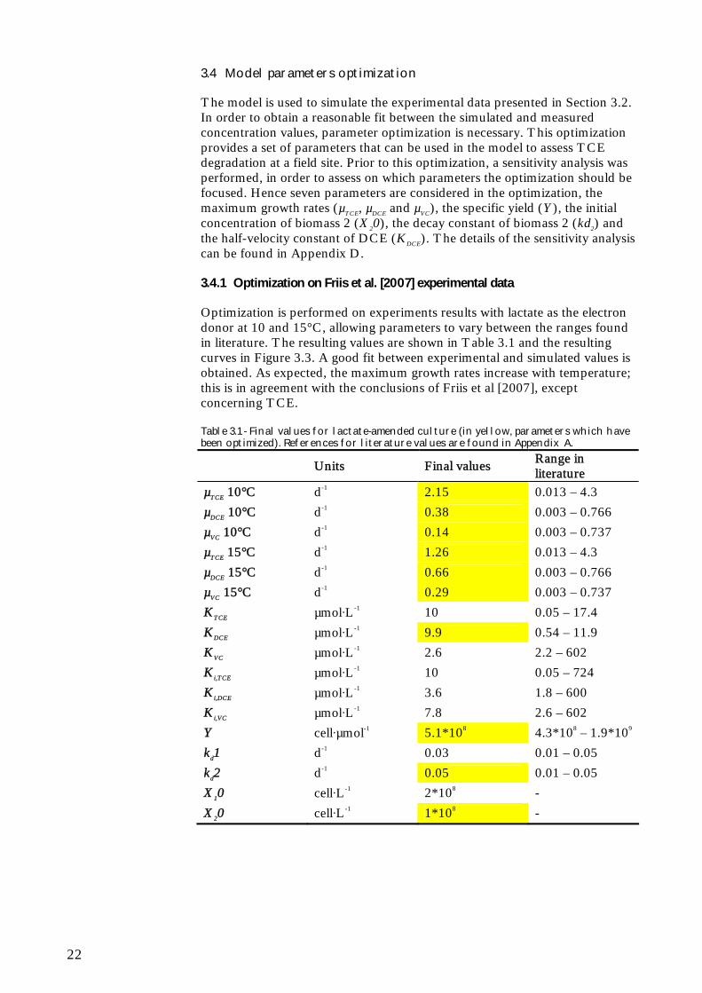
The model is used to simulate the experimental data presented in Section 3.2. In order to obtain a reasonable fit between the simulated and measured concentration values, parameter optimization is necessary. This optimization provides a set of parameters that can be used in the model to assess TCE degradation at a field site. Prior to this optimization, a sensitivity analysis was performed, in order to assess on which parameters the optimization should be focused. Hence seven parameters are considered in the optimization, the maximum growth rates (µTCE, µDCE and µVC), the specific yield (Y), the initial concentration of biomass 2 (X20), the decay constant of biomass 2 (kd2) and the half-velocity constant of DCE (KDCE). The details of the sensitivity analysis can be found in Appendix D. 3.4.1 Optimization on Friis et al. [2007] experimental data

Optimization is performed on experiments results with lactate as the electron donor at 10 and 15°C, allowing parameters to vary between the ranges found in literature. The resulting values are shown in Table 3.1 and the resulting curves in Figure 3.3. A good fit between experimental and simulated values is obtained. As expected, the maximum growth rates increase with temperature; this is in agreement with the conclusions of Friis et al [2007], except concerning TCE. Table 3.1 - Final values for lactate-amended culture (in yellow, parameters which have been optimized). References for literature values are found in Appendix A.

Units Final values Range in literature

µTCE 10°C d-1 2.15 0.013 – 4.3

µDCE 10°C d-1 0.38 0.003 – 0.766

µVC 10°C d-1 0.14 0.003 – 0.737

µTCE 15°C d-1 1.26 0.013 – 4.3

µDCE 15°C d-1 0.66 0.003 – 0.766

µVC 15°C d-1 0.29 0.003 – 0.737

KTCE µmol·L-1 10 0.05 – 17.4

KDCE µmol·L-1 9.9 0.54 – 11.9

KVC µmol·L-1 2.6 2.2 – 602

Ki,TCE µmol·L-1 10 0.05 – 724

Ki,DCE µmol·L-1 3.6 1.8 – 600

Ki,VC µmol·L-1 7.8 2.6 – 602

Y cell·µmol-1 5.1*108 4.3*108 – 1.9*109

kd1 d-1 0.03 0.01 – 0.05

kd2 d-1 0.05 0.01 – 0.05

X10 cell·L-1 2*108 -

X20 cell·L-1 1*108 -

23

Figure 3.3 - Experimental data vs. simulated curves with optimal parameters for lactate-amended culture, at 10 and 15 °C The experimental results with propionate as the electron donor are then simulated using the optimized values from Table 3.1 with for the growth rate as independent parameter that is optimized. As complete degradation down to ethene is not observed at 10°C, the optimization is performed on the results at 15°C only. The resulting maximum growth rate values are shown in Table 3.2. As expected, the maximum growth rates are lower than for lactate, except for TCE. Furthermore, the fit for propionate is poorer than for lactate. This may be due to the fact that propionate-amended system does not adhere to the model assumption of unlimiting substrate [Friis et al., 2007]. Nevertheless the time scale of TCE degradation in a propionate-amended culture is well simulated by the given parameters. Table 3.2 - Final values for propionate-amended culture (in yellow, parameters which have been optimized). References for literature values are found in Appendix A

Units Final values Range in literature

µTCE 15°C d-1 2.1 0.013 – 4.3

µDCE 15°C d-1 0.4 0.003 – 0.766

µVC 15°C d-1 0.1 0.003 – 0.737

KTCE µmol·L-1 10 0.05 – 17.4

KDCE µmol·L-1 9.9 0.54 – 11.9

KVC µmol·L-1 2.6 2.2 – 602

Ki,TCE µmol·L-1 10 0.05 – 724

Ki,DCE µmol·L-1 3.6 1.8 – 600

Ki,VC µmol·L-1 7.8 2.6 – 602

Y cell·µmol-1 5.1*108 4.3*108 – 1.9*109

kd1 d-1 0.03 0.01 – 0.05

kd2 d-1 0.05 0.01 – 0.05

X10 cell·L-1 2*108 -

X20 cell·L-1 1*108 -

24

Figure 3.4 - Experimental data vs. simulated curves for propionate-amended culture at 15 °C 3.4.2 Simulation of treatability study data– sand samples

As verification, the model is used to simulate laboratory experiments where sand and groundwater from Rugårdsvej field site are added. These conditions are closer to field conditions. In these experiments, electron donor (lactate or propionate) is added at day 0, while the dechlorinating biomass (KB-1 culture) is added at day 57. The details concerning the experimental set-up can be found in [Jørgensen et al., 2007b]. The initial bacteria concentration in the sample is not known and no prior information is available. However, it seems that this parameter is not very sensitive in the model (see Appendix D) so X10 (initial concentration of biomass population 1) is set to 8*104 cells/L in samples K and M and to 8*107 cells/L in sample L, as it is observed that TCE degrades much faster in this sample (see Figure 3.5). A rough estimate of the added dechlorinating biomass is performed. The culture is diluted 1000 times, resulting in an initial Dehalococcoides concentration between 107 and 108 cells/L. Lactate as electron donor Taking the optimized parameters from Table 3.1, only the initial concentration of biomass population 2, X20 is optimized for the samples K, L and M, given a value of 4.5*107 cell/L. The resulting curves are shown Figure 3.5. A reasonable fit is obtained for the different samples, indicating that the model describes these data sets well.

25

Figure 3.5 - Experimental data vs. simulated curves for lactate-amended culture, optimization only on X20 Propionate as electron donor Taking the optimized parameters from Table 3.2, with an initial biomass value X20 of 3*107 cell/L is used for the samples K, L and M. The resulting curves are shown in Figure 3.6. The simulation gives a reasonable fit for samples K and M but the result with sample L is not satisfying with respect to cis-DCE degradation to VC (slower in the experiment). Based on the lactate and propionate results, it appears that simulations are poorest for sample L. This can be due to the presence of competitive bacteria populations in high concentration, leading to limiting substrate conditions for dechlorination, which is not included in the model processes; so this sample does not correspond to the model assumptions.

26

Figure 3.6- Experimental data vs. simulated curves for lactate-amended culture, optimization only on X20 (initial biomass population)

3.5 Coupling to the transport model

The laboratory experiment “sub-model” allows definition of a set of differential equations to simulate the sequential dechlorination from TCE to ethene. This mathematical model can be combined with a transport model, in order to characterize TCE degradation and transport in the fractured clay system. To sets of kinetic parameters are defined depending on the electron donor characteristics (lactate or propionate).

27

4 Transport in the clay matrix

In this section, a model for contaminant transport in the clay matrix is developed. The model is applied to experimental data from a field site at Rugårdsvej.

4.1 Theory

Transport of the contaminant in the clay matrix is a very important process relative to risk assessment and remediation. The clay will act as a long-term contaminant source and the transport in this low permeability layer is often the limiting factor for remediation. Transport in low permeability layer, such as clay, is in most of the cases controlled by molecular diffusion, as advection/dispersion mechanisms are negligible because of the low permeability. The relative contribution of advection/dispersion and diffusion to solute transport can be evaluated with the Peclet number [Bear, 1979]:

*

e

vLP

D (3.1)

Where v is the average flow velocity (m/s), L is the characteristic length of the system (m) and D* is the molecular diffusion coefficient in the considered liquid (here water) (m2/s). In the studied system, the average flow velocity is defined by Darcy’s law:

mK iv

(3.2)

Where Km is the clay matrix hydraulic conductivity (m/s), i is the vertical hydraulic gradient through the clay matrix and is the matrix porosity. For such systems, the characteristic length L can be defined as the thickness of the clay layer. To insure the predominance of the molecular diffusion, the Peclet number should be smaller than 1 [Bear, 1972]. Given a free diffusion coefficient of 6.23*10-10 m2/s (corresponding to diffusion of TCE in water at 10°C, see Table 4.2), a porosity of 0.3, this condition corresponds to: 101 * 2 10 e m mP K iL D K iL (3.3) The matrix hydraulic conductivity for clay till is in the range 10-9 – 10-11 m/s in Denmark [Jørgensen et al., 1998], and the thickness can vary between 1 and 10 meters. Hence the hydraulic gradient should be smaller than 1 to insure Pe < 1, for Km = 10-9 m/s and L = 10 m (limit case). This high limit value for hydraulic gradient shows that the assumption of solute transport controlled by molecular diffusion will be valid in most of the cases with clay till. When the clay has a higher hydraulic conductivity (Km > 10-9 m/s), resulting from the presence of sand in the clay till for example, the assumption of negligible advection/dispersion should be reconsidered.

28

For solute transport controlled by molecular diffusion, the corresponding equation transport is [Fetter, 1998]:

C

R D Ct

(3.4)

Where R is the retardation factor, D is the effective diffusion coefficient (m2/s) and C is the contaminant aqueous concentration (mol/L). Retardation of contaminant is due to sorption to the sediment. Under the assumption of linear sorption, sorption can be represented by the linear sorption coefficient Kd (L/kg). The retardation factor can then be calculated with:

1 bdR K

(3.5)

Where ρb is the bulk density (kg/L) and is the porosity of the matrix material. Kd is a parameter which is difficult to measure, so it is usually estimated from the octanol-water partition coefficient KOW and the organic carbon fraction foc [Fetter, 1998], with the following Abduls formula for chlorinated solvents [Abdul et al., 1987]: log 1.04 log 0.84oc owK K (3.6)

d oc ocK K f (3.7) The effective diffusion coefficient can be calculated with: *D D (3.8) Where τ is the tortuosity coefficient and D* is the free diffusion coefficient in water (m2/s). The tortuosity coefficient is often estimated with the porosity, as it is a parameter difficult to measure with laboratory experiments. The tortuosity is related to the matrix porosity with the following equation [Parker et al., 1994]: p (3.9) Where values of the exponent p varies between 0.4 and 2 with an average of 1.1 for natural clays and clay tills [Parker et al., 2004]. Hence the tortuosity coefficient is often approximated to be equal to the total matrix porosity [Broholm et al., 1999 and Jørgensen et al., 2004].

4.2 Experimental data

Experimental data showing the transport of chlorinated ethenes in clay are scarce. Here the model is compared with data from experiments conducted on a field site at Rugårdsvej [Jørgensen et al. 2007b]. The data consists of core samples which were collected 5 months after injection of substrate and bacteria at the field site. Detailed profiles of chlorinated solvents, bacteria, electron donor and anion concentrations were collected.

29

Figure 4.1 - Core sample with fracture location The detailed concentration profiles as a function of the distance to the fracture are shown for different compounds in Figure 4.2. The distribution of chlorinated solvents is characterized by a diffusion profile with concentration decreasing from the matrix to the fracture (where degradation takes place). In the experiments substrate was injected in the fracture and Figure 4.2 shows a diffusion profile where the concentrations are decreasing with distance from the fracture.

Figure 4.2 - Chlorinated solvents (left) and acids in clay core taken 5 months after injection These experimental data are used to characterize the diffusive interaction between the fracture and the clay and to determine the key parameters, which control this process.

4.3 Modeling approach

In this section, a simple model is built to simulate the counter diffusion of chlorinated solvents from the matrix into the fracture, where degradation is assumed to take place.

30

4.3.1 Conceptual model

The aqueous concentration evolution in the matrix after injection of substrate and bacteria is modeled with a 1D-diffusion model.

Figure 4.3 - Conceptual model of counter diffusion out of the matrix into the fracture Given that each clay matrix block is separated by fractures, then there is a line of symmetry through the middle of each matrix block and the concentration can be modeled between the fracture and the middle of the block. The fracture aperture is assumed to be 2 cm and the clay block is modeled for a distance of 25cm from the fracture. Fast degradation is assumed to take place in the fracture and the concentration is set to zero at this boundary. No degradation is assumed to occur in the matrix, as in this first approach the bacteria (specific degraders) are assumed to be unable to move into the matrix, where pore size may be limited (see Section 4.3.4). The equations in the clay are:

2

2DCE DCE

DCE DCE

C CR D

t x

(3.10)

2

2VC VC

VC VC

C CR D

t x

(3.11)

As a result of the symmetry assumption, a zero concentration gradient condition is applied at the boundary of the system (corresponding to the middle of the clay block). Degradation is assumed to occur only in the aqueous phase and not in the sorbed phase, so the model is based on the aqueous concentration. However the measured concentrations are a total concentration, and so it is necessary to convert the aqueous concentration from the model into a total concentration. If sorption isotherms are linear as assumed above, then the total concentration Ctot (dissolved + sorbed amount of compound, µmol.kg-1 bulk) is:

Fracture

Core sample

Counter diff i

31

1tot w b d

bC C K (3.12)

Where Cw is the aqueous concentration (in µmol/L) and ρb is the bulk density (in kg/L). A constant initial concentration for DCE and VC is assumed and equal to the measured aqueous concentrations in the fracture before injection of substrate and bacteria. This aqueous concentration should correspond to the total concentration measured in the core sample at approximately 20 cm from the fracture (see Figure 4.2). 4.3.2 Parameters

Field specific data (measured or estimated) are taken from [Jørgensen et al., 2007a] and shown in Table 4.1. To complete the model additional parameters from the literature are needed and these are shown in Table 4.2. Other parameters can be calculated using the equations shown in the text and are shown in Table 4.3. Table 4.1 – Measured/assumed parameters for input in model [Jørgensen et al., 2007a]

Parameters Symbol Unit Value

Porosity - 0.25

Dry bulk density b kg/L 1.99

Wet bulk density tot kg/L 2.24

Organic carbon content foc - 0.002 Initial aqueous concentration DCE

Cini,DCE µmol/L 32

Initial aqueous concentration VC Cini,VC µmol/L 41

Table 4.2 - Parameters from literature for input in model


Free diffusion coefficient TCEa D*TCE m2/s 6.23*10-10

Free diffusion coefficient DCEa D*DCE m2/s 7.08*10-10

Free diffusion coefficient VCa D*VC m2/s 8.34*10-10

Octanol-water partition DCEb log(Kow-DCE) - 1.86

Octanol-water partition VCb log(Kow-VC) - 1.38 a from [US EPA, 2008] b from [Abdul et al., 1987]

32

Table 4.3 – Calculated parameters for input in the model


DCE sorption coefficient KdDCE L/kg 0.025

VC sorption coefficient KdVC L/kg 0.008

DCE retardation coefficient RDCE - 1.21

VC retardation coefficient RVC - 1.06

Tortuosity τ - 0.25

Diffusion coefficient DCE DDCE m2/s 1.77*10-10

Diffusion coefficient VC DVC m2/s 2.08*10-10 Initial total concentration DCE

Ctot,ini, DCE µmol/kg 4.26

Initial total concentration VC Ctot,ini, VC µmol/kg 4.81

From Table 4.3 it can be seen that the initial total concentration in the model is much lower than the concentrations measured on the core sample at a distance > 20cm from the fracture (see Figure 4.2, Ctot,ini,DCE ≈ 35 µmol/kg and Ctot,ini,VC ≈ 18 µmol/kg). As all parameters except for the sorption coefficients have been measured, the difference is due to an underestimation of the sorption coefficients using the empirical Abdul’s equation and the estimated fraction of organic compound (foc). This can be due to the fact that for chlorinated solvents, sorption on clay is not directly proportional to the organic carbon fraction [Allen-King et al., 1996]. In order to match the measured total concentrations, the sorption coefficients must be multiplied by 40, giving KdDCE = 1.04 L/kg and KdVC = 0.32 L/kg. Experiments conducted at DTU Environment on samples from several field sites (including Rugårdsvej) have given sorption coefficients for cis-DCE and VC around 0.8 and 0.3 L/kg respectively [Zhang, 2008, unpublished]. In these experiments, foc was found to be almost 10 times higher (foc = 0.017) than the estimated value from [Jørgensen et al., 2007a], but this higher value does not explain completely the higher sorption values measured. These new sorption coefficients are based on core samples analysis and sorption experiments in laboratory. Further research would be needed in this area to determine how the sorption coefficient can be estimated from organic carbon content and if a correction factor should be applied in a general contest. The retardation factor is a function of the sorption coefficient and a higher retardation factor value results in a slower diffusion of compounds out of the matrix and hence longer remediation times. Based on the newly estimated sorption coefficients, the retardation factor become: RDCE = 9.4 RVC = 3.6 4.3.3 Model results

The simulated concentration profiles with various Kd-values are shown in Figure 4.4 at a time of 5 months. The new sorption coefficients calculated above allow a better simulation of the profiles. However the simulated profile for DCE does not describe well the measured data from the core samples between 0.05 and 0.10 cm from the fracture. In this simple model it was assumed that no degradation occurs in the clay matrix. DCE reductive

33

dechlorination in the matrix would correspond to VC production, resulting in higher VC concentrations along the diffusion profile, and ethene production through VC dechlorination. But it has been seen in Figure 4.2 that no ethene is present in the matrix.

Total concentration in µmol/kg0 10 20 30 40

dist

ance

fro

m f

ract

ure

in m

0,00

0,05

0,10

0,15

0,20

0,25

DCE with Kd = 0.025 L/kg

VC with Kd = 0.008 L/kg

DCE with Kd = 1 L/kg

VC with Kd = 0.32 L/kg

measured DCEmeasured VC

Figure 4.4 - Simulated diffusion profiles after 5 months for different Kd-values The difference between the simulated and measured profiles may also be due to an incorrect estimation of one or more parameters. Of all parameters, the tortuosity is the one most probable to have been miss-estimated. Therefore the model was run with different values for τ between 0.06 and 0.57 (corresponding to p equal 2 and 0.4 respectively, see Equation (3.9)). The slopes of the diffusion profiles decrease with increasing tortuosity factor. A high tortuosity provides a better fit of the DCE concentration profile.

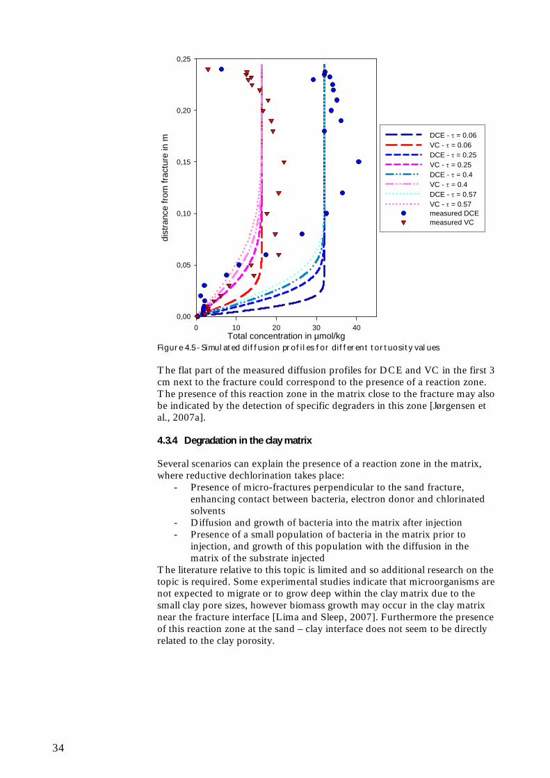
34

Total concentration in µmol/kg0 10 20 30 40

dist

ranc

e fr

om f

ract

ure

in m

0,00

0,05

0,10

0,15

0,20

0,25

DCE - = 0.06VC - = 0.06DCE - = 0.25VC - = 0.25DCE - = 0.4VC - = 0.4DCE - = 0.57VC - = 0.57measured DCEmeasured VC

Figure 4.5 - Simulated diffusion profiles for different tortuosity values The flat part of the measured diffusion profiles for DCE and VC in the first 3 cm next to the fracture could correspond to the presence of a reaction zone. The presence of this reaction zone in the matrix close to the fracture may also be indicated by the detection of specific degraders in this zone [Jørgensen et al., 2007a]. 4.3.4 Degradation in the clay matrix

Several scenarios can explain the presence of a reaction zone in the matrix, where reductive dechlorination takes place:

- Presence of micro-fractures perpendicular to the sand fracture, enhancing contact between bacteria, electron donor and chlorinated solvents

- Diffusion and growth of bacteria into the matrix after injection - Presence of a small population of bacteria in the matrix prior to

injection, and growth of this population with the diffusion in the matrix of the substrate injected

The literature relative to this topic is limited and so additional research on the topic is required. Some experimental studies indicate that microorganisms are not expected to migrate or to grow deep within the clay matrix due to the small clay pore sizes, however biomass growth may occur in the clay matrix near the fracture interface [Lima and Sleep, 2007]. Furthermore the presence of this reaction zone at the sand – clay interface does not seem to be directly related to the clay porosity.

35

4.4 Summary of the matrix sub-model

The transport of the chlorinated solvents in the matrix is characterized by the diffusion coefficient and the retardation factor. Two parameters have been shown to be controlling this process, the sorption coefficient, which may be underestimated with the foc approach, and the tortuosity coefficient. Furthermore the presence of a reaction zone in the matrix close to the fracture is suggested by the results of the model. However the processes responsible for this phenomenon have not been identified.

37

5 Coupling of the “sub-models”

In this section, the two sub-models described in Sections 0 and 1 are coupled in a unique numerical model, in order to simulate transport and degradation of TCE in a single fracture – clay matrix system. The model implementation is first described and the influence of the different parameters and configurations on the results is assessed.

5.1 Theory

5.1.1 Transport equations in matrix and fracture

In the model, we will consider a set of identical vertical fractures whose axes are parallel and equally spaced (Figure 5.1). Hence the fracture network is characterized by only two parameters, the fracture aperture 2b and the fracture spacing 2B. Fracture porosity f = b/B is generally used to characterize such fractured porous media [Freeze and McWhorter, 1997], f ranges between 10-4 and 10-2 for typical fractured sedimentary deposits [Parker et al., 1997]. A model is constructed with the following assumptions:

- Fracture width is much smaller than its length - Transverse diffusion and dispersion within the fracture assures

complete mixing across its width at all times - Transport within the matrix will be mainly by molecular diffusion (see

Section 4.1) - Transport along the fracture is much faster than transport within the

matrix - No adsorption on the fracture wall

Because of the symmetry of the system, we need to consider only one half of a fracture and one half of the intervening porous matrix. The transport processes in the system are described by two coupled equations (one 1D for the fracture and one 2D for the matrix), with the coupling being provided by concentration continuity along the interface. The differential equation describing transport along the fracture is [Sudicky and Frind, 1982]:

2

20f f f m

f f

C C C Qv D

t z z b

(4.1)

Where Cf is the aqueous concentration in the fracture (in µmol/L), vf is the groundwater velocity in the fracture (in m/s), Df is the hydrodynamic dispersion coefficient (in m2/s), Qm is the mass transfer flux from the fracture due to diffusion at the fracture-matrix interface (in µmol/s/m2) and b is the half aperture of the fracture (in m).

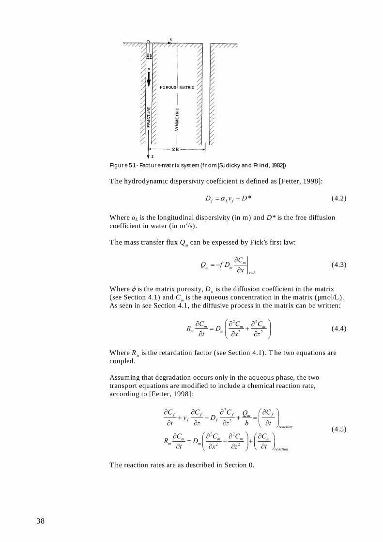
38

Figure 5.1 - Facture-matrix system (from [Sudicky and Frind, 1982]) The hydrodynamic dispersivity coefficient is defined as [Fetter, 1998]: *f L fD v D (4.2)

Where αL is the longitudinal dispersivity (in m) and D* is the free diffusion coefficient in water (in m2/s). The mass transfer flux Qm can be expessed by Fick’s first law:

mm m

x b

CQ D

xf

(4.3)

Where is the matrix porosity, Dm is the diffusion coefficient in the matrix (see Section 4.1) and Cm is the aqueous concentration in the matrix (µmol/L). As seen in see Section 4.1, the diffusive process in the matrix can be written:

2 2

2 2m m m

m m

C C CR D

t x z

(4.4)

Where Rm is the retardation factor (see Section 4.1). The two equations are coupled. Assuming that degradation occurs only in the aqueous phase, the two transport equations are modified to include a chemical reaction rate, according to [Fetter, 1998]:

2

2

2 2

2 2

f f f fmf f

reaction

m m m mm m

reaction

C C C CQv D

t z z b t

C C C CR D

t x z t

(4.5)

The reaction rates are as described in Section 0.

39

5.1.2 Determination of flow through fracture

SprækkeJAGG approach The flow through the fracture is estimated using the conceptual model employed in SprækkeJAGG [SprækkeJAGG, 2008]: the net precipitation that falls on the land surface will flow downwards through the fractures. Hence the water flow through a single fracture can be estimated with: 2fQ I B (4.6)

Where Qf is the water flow in the fracture per unit meter (m3/year/m), I is the net precipitation rate (m/year) and 2B is the distance between two fracture (m). Based on this approach, the fracture velocity, vf, can be calculated:

2

ff

Q bv I

b B (4.7)

This approach may be reasonable when the distance between two fractures is small, but it is unrealistic when B is large. Furthermore it can be noticed that with this definition, the flow in the fracture does not depend on its aperture.

Figure 5.2 – Definition of flow into fracture “Cubic law” approach In another model approach, the flow through the fracture can be estimated using the “cubic law” [McKay et al, 1998], where the volumetric flow is a function of the fracture aperture cubed: 2f fQ K b i (4.8)

Where i is the vertical hydraulic gradient along the fracture and Kf is the hydraulic conductivity of the fractures defined as

22

12f

gK b

µ

(4.9)

Where ρ is the fluid density (kg/m3), g is the gravitational acceleration (m/s2) and μ is the viscosity (Pa.s).

2b 2B

Net precipitation I

40

For a system of parallel fractures, the bulk hydraulic conductivity of the system Kb can be expressed as:

2

2 b f m

bK K K

B (4.10)

As Km << Kb, Equation (4.10) can be reduced to

322

2 2 12 b f

bb gK K

B B

(4.11)

The bulk hydraulic conductivity can be measured at a field site with slug tests and given an estimation of the fracture spacing, the average hydraulic fracture aperture can be calculated with:

3 122 2b B

g

(4.12)

Inserting (4.9) and (4.12) in (4.8) gives: 2 f bQ B K i (4.13)

The equation above has a similar form as Equation (4.6), where I is replaced by Kbi. Hence if the net precipitation rate I is equal to the bulk hydraulic conductivity Kb times the hydraulic gradient i (which is the case as long as both matrix and fractures are fully saturated and that the hydraulic conductivity of the matrix is very low), the two approaches will be equivalent. However the fracture aperture in SprækkeJAGG is not constrained by the other parameters of the systems and this can lead to unrealistic water balance in the clay till. Nevertheless it appears that the model is almost insensitive to the fracture aperture (see Section 5.2.5), so the two approaches will lead to similar results when the same water flow is applied as input with a given fracture spacing.

5.2 Single fracture/matrix model

5.2.1 Model set-up

The model domain is a rectangle which corresponds to half the matrix between two fractures. The transport equation (4.4) is defined in the domain, while the transport equation (4.1) is defined on the domain boundary, corresponding to the fracture location (Figure 5.3). The top and right boundaries are defined with a zero concentration gradient. The left boundary corresponds to continuity of concentration between fracture and matrix (Cm = Cf). The bottom boundary is also defined with a zero-concentration gradient, as it is assumed that the advective flux through the fracture is much more important than the diffusive flux that can be created at the bottom of the matrix (this assumption is documented in Section 5.2.3 and Appendix F).

41

Figure 5.3 - Model set-up The default parameters used for this model are summarized in Table 5.1. The free diffusion coefficients are taken from [US EPA, 2008]. The sorption coefficients are average values of experiments performed at DTU Environment on clay samples (see Section 4.3.3). The matrix porosity is a typical value for clay till and the dry bulk density is calculated based on the dry density of quartz (2.65 kg/L). The fracture longitudinal dispersivity is an assumed value, based on the value used in Sudicky and Frind [1982] and Therrien and Sudicky [1996]. Finally the fracture aperture and spacing are average values from several Danish sites, where 2b varies between 30 and 3000 µm and 2B varies between 0.005 and 1 m [Christiansen and Wood, 2006]. The model verification with an analytical solution can be found in Appendix E.

Thi

ckne

ss o

f th

e cl

ay la

yer

(hcl

ay)

Half fracture spacing (B)

2 2

2 2m m m

m m

C C CR D

t x z

2

20f f f m

f f

C C C Qv D

t z z b

42

Table 5.1 - Default transport parameters

Parameters Symbol Expression Value Unit Net recharge I 0.1 m/year Fracture spacing 2B 0.3 m Fracture aperture 2b 7*10-4 m Water velocity in fracture vf I*2B/(2b) 43 m/year Sorption coefficient TCE Kd_TCE 1 L/kg Sorption coefficient DCE Kd_DCE 0.7 L/kg Sorption coefficient VC Kd_VC 0.3 L/kg Dry bulk density b 2.65*(1-) 1.8 kg/L Matrix porosity 0.33 - Matrix tortuosity 0.33 - Retardation factor TCE R_TCE 1+b*Kd_TCE/ 6.5 - Retardation factor DCE R_DCE 1+b*Kd_DCE/ 4.8 - Retardation factor VC R_VC 1+b*Kd_VC/ 2.6 - Longitudinal dispersivity in f

L 0.1 m Free diffusion coef TCE D*_TCE 0.020 m2/year Free diffusion coef DCE D*_DCE 0.022 m2/year Free diffusion coef VC D*_VC 0.026 m2/year Fracture dispersion coef TCE Df_TCE L*vf+D*_TCE 4.3 m2/year Fracture dispersion coef DCE Df_DCE L*vf+D*_DCE 4.3 m2/year Fracture dispersion coef VC Df_VC L*vf+D*_VC 4.3 m2/year Matrix diffusion coefficient TCE

Dm_TCE D*_TCE* 0.0065 m2/year Matrix diffusion coefficient DCE

Dm_DCE D*_DCE* 0.0074 m2/year Matrix diffusion coefficient VC Dm_VC D*_VC* 0.0087 m2/year

5.2.2 Model outputs

An example of the model output for a simple case is explained. The default parameters are used and no degradation is assumed. The model simulates the flushing of the contaminant out of the matrix, by a flow of clean water in the fracture. The initial condition is defined with a uniform contaminant concentration in the whole matrix (for the influence of the initial conditions on the results, see Appendix G). The contaminant distribution changes with time are shown in Figure 5.4. The model is set up as shown in Figure 5.3. Each strip in Figure 5.4 represents a clay block of width 0.15 meter. The fracture is located on the left hand edge of each strip. Results show that the matrix is “cleaned” from the top-left corner to the bottom-right. Clean water enters the fracture (at the top left) and a concentration gradient is formed, resulting in counter diffusion from the matrix into the fracture. The cleaning starts at the top of the matrix where rain water enters. The water then becomes more contaminated as it flows downwards along the fracture. The contaminant concentration in the water flowing from the fracture outlet is shown in Figure 5.5, as well as the change in the total contaminant mass (total mass of contaminant divided by initial mass). It takes around 250 years to flush all contaminant out of the matrix and to reduce significantly the contaminant concentration at the fracture outlet. This long time scale is due to the very slow transport of the contaminant in the matrix, as it is controlled by

43

molecular diffusion. Similar time scale has been reported in Reynolds and Kueper [2002] and Falta [2005].

Figure 5.4 - Contaminant distribution in the matrix for different times. Each strip represents a clay block of width 0.15 meter (corresponding to 0.3 meters between fractures). No degradation

time in years0 50 100 150 200 250

Aqu

eous

C/C

0 in

%

0

20

40

60

80

100

M/M

0 in

%

0

20

40

60

80

100

Figure 5.5 - Concentration at the fracture outlet (red - left axis) and total mass remaining in the system (blue – right axis). No degradation

44

5.2.3 Advective/Diffusive transport through fracture and matrix

The diffusive flux which can be created at the bottom of the matrix is assessed and compared with the advective contaminant flux at the fracture outlet, for different fracture aperture/fracture spacing configurations. In scenario 1, all contaminant leaves the system through the fracture outlet (as a zero-concentration gradient boundary is defined at the bottom of the matrix), while for scenario 2, a zero concentration boundary is defined at the bottom of the matrix, allowing contaminant to leave the system by diffusion. The conceptual models resulting from these two scenarios are shown in Figure 5.6.

Figure 5.6 - Conceptual models for the two transport scenarios In both configurations, the flux through the matrix is minor, but differences increase when the fracture spacing is reduced, from 9% for 2B = 1m and up to 23 % for 2B = 0.005 m. An example of the contaminant fluxes for fracture spacing 2B = 0.05m is shown in Figure 5.7, where the diffusive flux is less than 20 % of the total contaminant flux.

Time in years0 50 100 150 200

flux

in m

mo

l/yea

r/m

0,0

0,2

0,4

0,6

0,8

1,0flux through fractureflux through matrixTotal flux

Figure 5.7 - Flux at the output of the system in scenario 2 (for 2b = 10-4 m and 2B = 0.05 m)

Advection

Diffusion

No flow

Advection Diffusion

Diffusion

Scenario 1 Scenario 2

45

Although the diffusive flux can represent up to 25 % of the total flux, it does not seem to change the model results, in term of total contaminant flux from the system and the contaminant distribution in the matrix. These results are obtained by using the transport coefficients of TCE. It is expected that the diffusive flux would be more important in the case of VC, as the diffusion coefficient is higher. Nevertheless it is assumed that the total contaminant flux will also remain the same. Therefore it was decided to use only scenario 1, where the only flux out of the system is the contaminant flux through the fracture outlet. More results and details can be found in Appendix F. 5.2.4 Degradation scenarios

As explained in Section 4.3.4, the results from field samples and literature studies have shown dechlorination may occur in a reaction zone near the high permeability sand zone (fractures), but no biomass transport or growth is expected deep within the clay matrix. Hence different scenarios need to be considered relative to degradation location:

- No degradation occurs in the system - Degradation occurs only in the high permeable zone, i.e. the fractures - A reaction zone is formed at the clay – fracture interface, where

degradation is also taking place - Degradation in the whole matrix

The last scenario is not likely to be realistic but is used to assess a “best case” relative to degradation. In the absence of literature data, the degradation zone is assumed to be extended up to 0.05 m inside the clay matrix, corresponding to observations at Rugårdsvej field site. However the biomass growth in this reaction zone is restricted by pore size limitations [Lima and Sleep, 2007] and cannot be simulated in the same way as the biomass growth in the fracture. For the simplicity of the model, the biomass will be assumed to be constant both in the fracture and matrix, with a concentration of 108 cells/L, this concentration corresponds to values measured in the field after injection [Miljøstyrelsen, 2008]. These four scenarios are applied to the base case configuration with the transport parameters in Table 5.1, while the parameters relative to chlorinated solvents dechlorination are taken from Table 3.2 in Section 3.4.1. Finally a homogenous initial aqueous TCE concentration of 100 mmol/m3 is applied (equal to 13139 µg/L).

46

time in years0 50 100 150 200 250 300

M/M

0 in

%

0

20

40

60

80

100no degradationdegradation in fracture onlydegradation in fracture and reaction zone in matrixdegradation fracture and in the whole matrix

Figure 5.8 - Remaining total contaminant (TCE+DCE+VC+ETH) mass in the system for the four degradation scenarios

time in years0 50 100 150 200 250 300

Aqu

eou

s C

/C0 in

%

0

20

40

60

80


Figure 5.9 –TCE concentration at the fracture outlet for the three degradation scenarios The scenario with degradation in the fracture only does not differ much from the scenario without degradation, especially concerning the mass removal rate in the system. This is due to the fact that the contaminant downward transport in the fracture, controlled by the groundwater velocity, is much higher than the degradation rate. Therefore the contaminant has no time to be degraded once it has reached the fracture (from counter diffusion from the matrix) and the production of daughter products (DCE and VC) is very limited (see Figure 5.10 - left). On the contrary in the presence of a reaction zone at the matrix – fracture interface, daughter products are formed (see Figure 5.10 - middle) and the mass removal occurs significantly faster (see Figure 5.8). As expected, under the assumption of degradation in the whole

47

matrix, the mass removal is much faster. Ethene concentration is not displayed on the graphs but is produced by VC reductive dechlorination.

degradation in fractureand reaction zone in matrix

time in years50 100 150 200 250

0

20

40

60

80

100

degradation in fracture only

time in years50 100 150 200 250

Aq

ueou

s C

/C0

in %

0

20

40

60

80

100TCE - no degrTCEDCEVC

degradation in fractureand in the whole matrix

time in years50 100 150 200 250

0

20

40

60

80

100

Figure 5.10 – TCE, DCE and VC concentrations at the fracture outlet for the three degradation scenarios (compared with TCE for the case without degradation) Finally, looking at the total chlorinated solvents concentration (TCE + DCE + VC, as ethene is a non-toxic compound) at the fracture outlet for the four different scenarios (see Figure 5.11), the peak concentration in case of degradation takes place several years after the beginning of remediation. This is because of the fact that the daughter products can move more easily from the matrix than TCE, as they have higher diffusion coefficients and lower retardation factors (see Table 5.1). Once formed in the matrix, the daughter products can therefore reach the fracture faster than TCE. This peak concentration has not been noted in the literature, because the same diffusion and sorption coefficients for different compounds have been applied [Sun and Buscheck, 2003].

48

Time in years0 50 100 150 200 250

Aqu

eous

Cto

tal/C

tota

l0 in

%

0

20

40

60

80

100

120

140

160no degradationdegradation in fracture onlydegradation in fracture and in reaction zone in matrixdegradation in fracture and in the whole matrix

Figure 5.11 - Total chlorinated concentration (TCE + DCE + VC) at the fracture outlet for the four scenarios 5.2.5 Sensitivity analysis

A sensitivity analysis is performed on the independent parameters of the model, using the transport and degradation parameters from the base case scenario and applying the third degradation scenario (degradation in the fracture and in the reaction zone in the matrix). Each parameter is varied by +/- 20%. In order to compare the different simulations, the initial concentration is corrected in order to maintain the same initial total mass in the system (158 mmol). By comparing the time to remove 90 % of the initial contaminant mass, it appears that the most sensitive parameters are the matrix porosity, the net recharge, the fracture spacing and the TCE sorption coefficient, while the least sensitive are the fracture aperture and longitudinal dispersivity in fracture. More detailed results can be found in Appendix I.

49

Table 5.2 - Sensitivity index for variation of +/- 20% of the parameters (transport parameters in orange and degradation parameters in green)

Parameter M<10% Mini

Matrix porosity 55.0 Net recharge 52.5 Fracture spacing 42.5 Sorption coefficient TCE 35.0 Sorption coefficient DCE 20.0 Specific yield 20.0 Initial biomass 20.0 Exponent p 10.0 Max growth rate DCE 10.0 Half velocity coefficient DCE 7.5 Sorption coefficient VC 5.0 Max growth rate TCE 5.0 Max growth rate VC 5.0 Fracture aperture 0.0 Longitudinal dispersivity in fracture 0.0

5.3 Aquifer model

5.3.1 Presentation of model

The aquifer model aims at simulating the contaminant fate in a high permeability aquifer located under the clay system. In this model the clay system acts as a contamination source for the aquifer. The aquifer is represented by a vertical cross-section, assuming a groundwater flow in one horizontal direction. The model considers two-dimensional steady flow modeled with a two-dimensional advection and dispersion transport equation. Furthermore, considering the long time scale resulting from the clay system model (several hundreds of years) compared with the relatively fast transport time in the groundwater, the transport model is assumed to be at steady state (the flux from the source is assumed to change very slowly compared to the residence time in the aquifer). For a clay system with vertical fractures down to the bottom, the aquifer can be considered as a leaky aquifer and the conceptual model with the main parameters is shown in Figure 5.12.

50

Figure 5.12 – Conceptual aquifer model for sand aquifer located under the clay system W is the source width K is the aquifer hydraulic conductivity I is the recharge rate aq is the aquifer porosity The hydraulic model is described by .( ) 0K h (4.14) which is subject to the boundary conditions:

1

2

0

,

0,

200,

botz z

top

h

z

h Ix z

z Kh x z h

h x z h

(4.15)

However in the clay model it was assumed that all water flows down in the fractures, the recharge flow is here distributed with width (see top boundary definition in equation). This is reasonable given the mixing of the water at the top boundary. The groundwater velocity is obtained using Darcy’s Law:

aq

Kv h

(4.16)

The contaminant transport model is given by . . . 0v C D C (4.17)

Recharge I

Flow direction

aq K

ztop

zbot

200m

Con

stan

t he

ad h

1

Source x=5 to 5+W m

0m

Con

stan

t he

ad h

2

Impermeable

51

with

i jij T ij L T

v vD v

v (4.18)

where

01

i jij i j

In such system, the model transport is insensitive to the longitudinal dispersivity αL [Prommer et al., 2006], so the dispersion tensor reduced to:

i jij T ij T

v vD v

v (4.19)

The transport model is subject to the initial and boundary conditions

,

0 0 /

5 5

0

0, 0 /

, 0

200, 0

top

top

aq zz z f out

z z

aq zz z

z z

bot

C t mol L

CD v C C I for x W

z

CD v C otherwise

z

C z mol L

Cx z z

zC

zz

(4.20)

Where Cf,out is the contaminant concentration at the fracture outlet (results from the clay system model). The clay layer source is defined as a specified-flux condition to ensure a proper contaminant mass balance [Van Genuchten and Alves, 1982]. As a result, the concentration at the top boundary is not equal to the concentration at the bottom of the clay system (concentration at the fracture outlet), but all of the contaminant that leaves the clay source enters the aquifer. For clay system with no vertical fractures, the aquifer can is confined and the recharge rate I = 0 m/year. In this case the flow and transport equations remain the same, but the boundary condition at the source is changed to:

5 5

0

top bot

top

maq zz m m

z z z z

aq zzz z

CCD D for x W

z z

CD otherwise

z

(4.21)

Where Cm is the concentration in the clay matrix.

52

5.3.2 Model outputs

This model is used to assess the maximal concentration along a cross-section at a certain distance L from the source (Caq,L,max). The main output from this model is the dilution factor df, which is defined as the ratio between the maximum concentration in the aquifer at the distance L and the concentration at the fracture outlet (in case of fracture), or the ratio between the maximum concentration in the aquifer at the distance L and the contaminant diffusive flux through the matrix (when there is no vertical fracture):

, ,max

,

, ,max

bot

aq L

f out

aq L

mm m

z z

Cdf incaseof vertical fracture

C

Cdf incaseof novertical fracture

CD

z

(4.22)

The distance from the source to the point of compliance (POC) is defined in Denmark as one year of groundwater transport (and maximum 100 m from the source) as specified in “Oprydning på forurenede lokaliteter” [Miljøstyrelsen, 1998]. In order to have the parameter L (distance between the middle of the source to the measurement point) independent of the other model parameters (K, I, hydraulic gradient, etc…), L is defined to 100 m (and not as one year of transport). An example of the model output is given for the following parameters:

- Hydraulic conductivity K = 2000 m/year (=6.3*10-5 m/s) - Recharge rate I = 200 mm/year - Hydraulic gradient i = 2 % - Effective porosity aq = 0.3 - Vertical transverse dispersvity T = 0.005 m - Source width W = 30 m - Cfract, out = 100 mmol/m3

Figure 5.13 - Contaminant concentration in the aquifer at steady-state

53

The contaminant concentration in the aquifer reaches a maximum value of 39 µmol/L, but decreases fast along the flow line, and is less than 10 % of the fracture concentration at 100 meters from the source (see Figure 5.14).

dilution factor in %0 2 4 6 8 10

De

pth

in m

ete

rs

0

1

2

3

4

5

Figure 5.14 - Dilution factor along the cross-section at 100 m from the source The concentration distribution in the aquifer is a function of the “flow factor”, defined as the ratio of the recharge rate (I) and the mean specific discharge (=K*i). The sensitivity analysis performed shows in addition to the flow factor, the model is sensitive to the source width and the vertical transverse dispersivity. The detailed results can be found in Appendix K.

5.4 Improving the modeling tool

This modeling tool was developed to characterize the main processes and the key parameters controlling the transport and degradation in a fractured clay till. With a single fracture – clay matrix model it was possible to assess the clean-up times for different configurations and degradation scenarios. However this model is still relatively simple and could be improved by the addition of other processes, notably in the dechlorination model. The introduction of biomass growth and decay could be interesting, even if it is possible to assume that a steady-state is reached relatively fast. Furthermore the limiting substrate condition and substrate concentration could be implemented, resulting in a more realistic modeling of the real system behavior. As explained in Section 3.1, the fermentation process, production of electron donor (here generally hydrogen) from the fermentation for the injected substrate, is also an important process in the system. The geometry of the model could also be improved by taking into account the presence of horizontal fractures, sand layers and sand lenses and considering heterogeneous fracture networks, which are closer to the real cases. Finally some studies need to be done in case the advective transport in the clay matrix can not be neglected, for example in the present of a high sand content in the clay till.

55

6 Modeling tool - case-study

6.1 Introduction

In order to apply the modeling tool, some important key parameters have to be known. Hence a good geological characterization, especially concerning the fractures in the clay system, is crucial to be able to apply the model. As presented in Miljøstyrelsen [2008], the geological characterization of the clay till is often poor at the different field sites investigated and further work is needed to obtain the relevant parameters. However an extended characterization of the geology at the field site Vadsbyvej has been performed with focus on the fractures in the clay till [Christiansen and Wood, 2006]. This field site will be used to illustrate an initial application of the modeling tool. In the third phase, the model will be applied to 2-3 sites.

6.2 Presentation of the site

The part is based on site characterization of [Region Hovedstaten, 2007], a updated version of this report (with a new mass estimation) can be found in [Region Hovedstaten, 2008], but has not been used. A more detailed model of this field site will be presented in the third report of this project. The presence of a chemical depot from 1973 resulted in soil and groundwater contamination with PCE, TCE, 1,1,1-TCA, BTEX, pesticides, acetone and isopropanol. The source is located in the upper clay till, where soil concentration up to 56 mg TCE/kg and water concentration up to 90 mg VC/L are found [Region Hovedstaten, 2007]. A sketch of the geology is shown in Figure 6.1. For more details on Vadsbyvej, see [Miljøstyrelsen, 2008] and [Region Hovedstaten, 2007].

Figure 6.1- Conceptualization of the local geology in the Vadsby area, from [Christiansen and Wood, 2006]

56

6.2.1 Characterization of the clay system

Vertical fractures are not expected to extend very much deeper than 6 meters below surface (top of the saturated zone), based on the thickness of the saturated clay till and field observations. In this project, we are focusing on transport in the saturated zone, so below the fractured zone. Therefore, the clay till at this site may be considered as a block, with no vertical fractures traversing the entire depth of the till deposit. This corresponds to scenario 3, as defined in Figure 2.2 in Section 2.1.1. In such a system, the contaminant is transported by diffusion in the matrix. It is expected that some horizontal sand lenses and fractures are present in the clay till but these pathways are disregarded in this model. The physical properties of the clay till are:

- Porosity = 0.3 - Dry bulk density b = 1.96 kg/L - Clay till thickness hclay = 10 m

6.2.2 Characterization of the source

The contamination at Vadsbyvej consists in two separate hotspots. In this report, we are focusing on hotspot 1. The source was divided into five zones, and the total mass of chlorinated ethenes is given for each zone. In this project we disregard the first zone, corresponding to the unsaturated zone and the last zone corresponding to the residual phase. Only three zones remain in the calculations, where the total mass of chlorinated ethenes is distributed among TCE, DCE and VC based on the average distribution of contaminant in the source. These total concentrations are then converted to aqueous concentrations. In the absence of field data regarding the sorption coefficient or the fraction of organic carbon, the sorption coefficients are calculated assuming foc = 1.5 % (KdTCE = 0.93 L/kg, KdDCE = 0.18 L/kg and KdVC = 0.06 L/kg). This foc value is large compare to standard value, but as explained in Section 1 and noted in Region Hovedstaden [2007], sorption on clay till is in general higher than the one calculated with the standard foc value. The source is assumed to have a parallelepiped shape, where the length is equal to the width. The concentrations in the source are modeled as uniform concentrations (values in row Total in Table 6.2). The concentrations given in the two tables are total aqueous and sorbed concentrations and the NAPL phase is neglected. Table 6.1 - Source zones characteristics

Area Depth Total mass

TCE DCE VC TCE DCE VC

m2 mbs kg kg kg kg g/L g/L g/L

Zone 1

100 5 – 10 56 42 11.76 2.24 0.0840 0.0235 0.0045

Zone 2

60 10 – 13

2.6 1.93 0.54 0.10 0.0107 0.0030 0.0006

Zone 3

20 13 – 15

4.19 3.14 0.88 0.17 0.0785 0.0220 0.0042

Total 100 5 – 15 62.8 47.07 13.18 2.51 0.0471 0.0132 0.0025

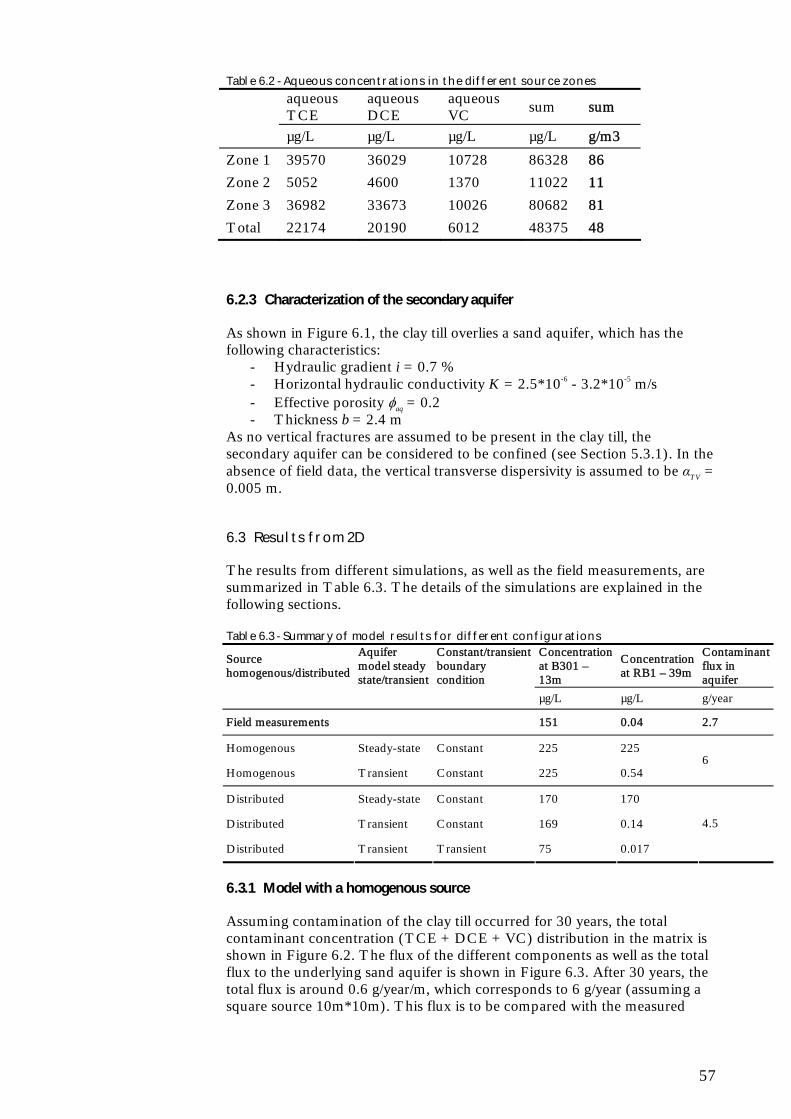
57

Table 6.2 - Aqueous concentrations in the different source zones

aqueous TCE

aqueous DCE

aqueous VC

sum sum

µg/L µg/L µg/L µg/L g/m3

Zone 1 39570 36029 10728 86328 86

Zone 2 5052 4600 1370 11022 11

Zone 3 36982 33673 10026 80682 81

Total 22174 20190 6012 48375 48

6.2.3 Characterization of the secondary aquifer

As shown in Figure 6.1, the clay till overlies a sand aquifer, which has the following characteristics:

- Hydraulic gradient i = 0.7 % - Horizontal hydraulic conductivity K = 2.5*10-6 - 3.2*10-5 m/s - Effective porosity aq = 0.2 - Thickness b = 2.4 m

As no vertical fractures are assumed to be present in the clay till, the secondary aquifer can be considered to be confined (see Section 5.3.1). In the absence of field data, the vertical transverse dispersivity is assumed to be αTV = 0.005 m.

6.3 Results from 2D

The results from different simulations, as well as the field measurements, are summarized in Table 6.3. The details of the simulations are explained in the following sections. Table 6.3 - Summary of model results for different configurations

Source homogenous/distributed

Aquifer model steady state/transient

Constant/transient boundary condition

Concentration at B301 – 13m

Concentration at RB1 – 39m

Contaminant flux in aquifer

µg/L µg/L g/year

Field measurements 151 0.04 2.7

Homogenous Steady-state Constant 225 225

Homogenous Transient Constant 225 0.54 6

Distributed Steady-state Constant 170 170

Distributed Transient Constant 169 0.14

Distributed Transient Transient 75 0.017

4.5

6.3.1 Model with a homogenous source

Assuming contamination of the clay till occurred for 30 years, the total contaminant concentration (TCE + DCE + VC) distribution in the matrix is shown in Figure 6.2. The flux of the different components as well as the total flux to the underlying sand aquifer is shown in Figure 6.3. After 30 years, the total flux is around 0.6 g/year/m, which corresponds to 6 g/year (assuming a square source 10m*10m). This flux is to be compared with the measured

58

chlorinated ethenes flux at the field site of around 2.7 g/year [Region Hovedstaden, 2007].

Figure 6.2 - Contaminant distribution in the clay till for a uniform source

time in years0 5 10 15 20 25 30

Flu

x in

g/y

ear/

m

0,0

0,1

0,2

0,3

0,4

0,5

0,6

0,7TCEDCE VCTotal flux

Figure 6.3 - Contaminant flux to the underlying aquifer The simulated total contaminant flux (0.6 g/year/m) is specified at the source boundary in the underlying aquifer model. The concentration for the two cross-sections shown in Figure 6.5 (corresponding to monitoring wells B301 and RB1 at 13 and 40 meters from the source respectively, see Figure 6.4) is averaged over the whole thickness, as the two wells are fully penetrating the secondary aquifer:

59

CB301 = 225 µg/L CRB1 = 225 µg/L

Figure 6.4 - Plan view of the source and monitoring wells These values should be compared with the total observed concentration of chlorinated ethenes at the two wells (the summation is made on the µg/L values): CB301 = 151 µg/L CRB3 = 0.04 µg/L

Figure 6.5 - Concentration in the aquifer for steady-state simulation With these two simple models, it is possible to estimate the order of magnitude of the contaminant flux to the secondary aquifer as well as the concentration in the aquifer. However it has been seen that the concentration is overestimated. Therefore a more realistic model for the contaminant distribution in the source and transient character of the aquifer model is set-up in the next section. 6.3.2 Distributed source concentration and transient model

Improvement of the source model In order to improve the accuracy, a more realistic model of the source area can be set up, where the source is divided into three zones. Inside each of these zones, the concentrations are assumed to be homogenous (see values in

Flow direction

B301RB1

0 10 20 40 30 Distance from the source in meters

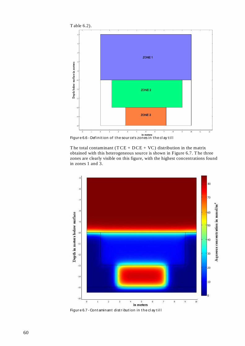
60

Table 6.2).

Figure 6.6 - Definition of the source's zones in the clay till The total contaminant (TCE + DCE + VC) distribution in the matrix obtained with this heterogeneous source is shown in Figure 6.7. The three zones are clearly visible on this figure, with the highest concentrations found in zones 1 and 3.

Figure 6.7 - Contaminant distribution in the clay till

61

The flux of the different components as well as the total flux to the underlying sand aquifer is shown in Figure 6.8. After 30 years, the total flux is around 0.45 g/year/m, which corresponds to 4.5 g/year (assuming a square source 10m*10m).

time in years0 5 10 15 20 25 30

Flu

x in

g/y

ear

/m

0,0

0,1

0,2

0,3

0,4

0,5TCEDCEVCTotal flux

Figure 6.8 - Contaminant flux to the underlying aquifer Improvement of the aquifer model The low hydraulic gradient and conductivity implies a relatively low velocity in the aquifer (around 3.5 m/year), therefore the steady-state model may overestimate the concentration in the aquifer. Hence a transient model may be more appropriate for the aquifer model. Two transient models are set-up, one with a constant flux boundary (0.45 g/year/m) and the other with a transient flux boundary condition: 0.45*t/30 g/year/m, where t is the time in years. This transient condition is a simple linear fit to the red curve in Figure 6.8. The average concentration (over the whole thickness) for the two cross-sections (corresponding to two monitoring wells) is: CB301 = 169 µg/L CRB1 = 0.14 µg/L for the constant boundary CB301 = 75 µg/L CRB1 = 0.017 µg/L for the transient boundary The distributed source model combined with a transient aquifer model compare better the total observed concentration of chlorinated ethenes at wells B301 and RB3: CB301 = 151 µg/L CRB1 = 0.04 µg/L

62

Figure 6.9 - Concentration in the aquifer at t=30 years with a constant boundary condition

Figure 6.10 - Concentration in the aquifer at t=30 years with a transient boundary condition The presence of the three zones in the source area does not significantly change the results. However the use of a transient model for the aquifer allows a better simulation of the concentration in the aquifer and the real extent of the plume. The model results obtained in the different configuration are summarized in Table 6.3 at the beginning of this section. This model is a simple attempt to represent Vadsbyvej field site, and would need some improvements to be more realistic. Mainly the presence of horizontal sand lenses, observed at the field site, should be implemented in the mode, in order to have a better simulation of the contamination distribution in the source zone and hence be able to predict the future developments of this contamination zone and the contaminant flux to the aquifer.

6.4 Application of the modeling tool to other real cases

In the third phase of this project, the modeling tool developed in this report will be applied to other field sites. For the cases, where reductive dechlorination is used as remediation technology, it will be possible to verify the model accuracy. For the cases the model will be used to assess the potential of using reductive dechlorination as a remediation technology with the given field site conditions.

63

6.5 Application of the modeling tool to real cases

In the third phase of this project, the modeling tool developed in this report will be applied to several Danish field sites. For the cases, where reductive dechlorination is used as remediation technology, it will be possible to verify the model accuracy. For the other cases the model will be used to assess the potential of using reductive dechlorination as a remediation technology with the given field site conditions.

65

List of references

Abduls A.S., Gibson T.L and Rai D.N., 1987, Statistical correlations for predicting the partition coefficient for nonpolar organic contaminants between aquifer organic carbon and water, Hazardous waste & hazardous materials, 4, 211-222. Allen-King, R.M., Groenevelt, H., Warren, C.J., og Mackay, D.M., 1996, Non-linear chlorinated solvent sorption in 4 aquitards, Journal of Contaminant Hydrology, 22, 203-221. Andrews J.F., 1968, A Mathematical Model for the Continuous Culture of Microorganisms Utilizing Inhibitory Substrates, Biotechnology and Bioengineering, vol. 10, no. 6, pp.707-723 Bagley D.M., 1998, Systematic approach for modeling tetrachloroethene biodegradation, Journal of environmental engineering, pp.1075-1086 Bear J., 1979, Hydraulics of groundwater, McGraw-Hill, New York, 567 pp. Berkowitz B., 2002, Characterizing flow and transport in fractured geological media: A review, Advances in Water Resources 25, 861–884. Bjerg P., Hansen M.H., Christiansen C., Scheutz C., Broholm M.M., 2006, Anaerob deklorering op oprensing af lavpermeable aflejringer, Københavns Amt, sara.er.dtu.dk Broholm M.M., Broholm K., Arvin E., 1999, Diffusion of heterocyclic compounds from a complex mixture of coal–tar compounds in natural clayey till, Journal of Contaminant Hydrology 39, 227–247 Christ J.A. and Abriola L.M., 2007, Modeling metabolic reductive dechlorination in dense non aqueous phase liquid source-zones, Advances in Water Resources 30, pp.1547–1561 Christiansen C. and Wood J. S. A. (2006), Environmental fracturing in clay till deposits, Master’s thesis, Danmarks Tekniske Universitet. Chu M., Kitanidis P.K. and McCarty P.L., 2004, Possible factors controlling the effectiveness of bioenhanced dissolution of non-aqueous phase tetrachloroethene, Advances in Water Resources 27, pp.601–615 Clapp L.W., Semmens M., Novak P.J. and Hozalski R.M., 2004, Model for in situ perchloroethene dechlorination via membrane-delivered hydrogen, Journal of Environmental Engineering, pp.1367-1381 Cupples A.M., Spormann A.M. and McCartyP.L., 2003, Growth of a Dehalococcoides-Like Microorganism on Vinyl Chloride and cis-Dichloroethene as Electron Acceptors as Determined by Competitive PCR, Applied and Environmental Microbiology, Vol. 69, No. 2, pp.953–959

66

Cupples A.M., Spormann A.M. and McCarty P.L., 2004a, Vinyl Chloride and cis-Dichloroethene Dechlorination Kinetics and Microorganism Growth under Substrate Limiting Conditions, Environmental Science & Technology, vol. 38, no. 4, pp.1102-1107 Cupples A.M., Spormann A.M. and McCarty P.L., 2004b, Comparative Evaluation of Chloroethene Dechlorination to Ethene by Dehalococcoides-like Microorganisms, Environmental Science & Technology, vol. 38, no. 4, pp. 4768-4774 Dennis P., Technical manager at Sirem, Ontario, Canada Duhamel M., Wehr S.D., Yu L., Rizvi H., Seepersad D., Dworatzek S., Cox E.E. and Edwards E.A., 2002, Comparison of anaerobic enrichment cultures maintained on tetrachloroethene, trichloroethene, cis-dichloroethene and vinyl chloride, Water Research, 36(17), pp. 4193-4202 Falta R.W., 2005, Dissolved chemical discharge from fractured clay aquitards contaminated by DNAPLs, Dynamics of fluids and transport in fractured rock, Geophysical Monograph Series 162. Fennell D.E. and Gossett J.M., 1998, Modeling the Production of and Competition for Hydrogen in a Dechlorinating Culture, Environmental Science & Technology, vol. 32, no. 16, pp. 2450 -2460 Fjengjun Z., 2008, Report of the sorption experiment of PCE, TCE, Cis-DCE and VC, DTU Environment, unpublished Fetter C.W., 1998, Contaminant hydrogeology, 2nd edition, MacMillan Publishing Company, New York. Freeze R.A. and McWhorter D.B., 1997, A framework for assessing risk reduction due to DNAPL mass removal from low-permeability soils, Ground Water 35(1), 111-123. Friis A.K., 2006, The potential for reductive dechlorination after thermal treatment of TCE-contaminated aquifers, PhD Thesis, DTU Environment. Friis A.K., Heimann, Jakobsen, Albrechtsen, Cox and Bjerg, 2007, Temperature dependence of anaerobic TCE-dechlorination in a highly enriched Dehalococcoides-containing culture, Water research, 41, pp.355-364 Garant H. and Lynd L., 1998, Applicability of Competitive and Noncompetitive Kinetics to the Reductive Dechlorination of Chlorinated Ethenes, Biotechnology and Bioengineering, vol. 57, no. 6, pp.751-755 Haston Z.C. and McCarty P.L., 1999, Chlorinated Ethene Half-Velocity Coefficients (KS) for Reductive Dechlorination, Environmental Science & Technology 33 (2), pp. 223 -226 He J., Sung Y., Dollhopf M.E., Fathepure B.Z., Tiedje J.M. and Löffler F.E., 2002, Acetate versus Hydrogen as Direct Electron Donors To Stimulate the Microbial Reductive Dechlorination Process at Chloroethene-Contaminated Sites, Environmental Science & Technology 36 (18), pp. 3945-3942.

67

Heimann A.C., Friis A.K. and Jakobsen R., 2005, Effects of sulfate on anaerobic chloroethene degradation by an enriched culture under transient and steady-state hydrogen supply, Water Research 39, pp. 3579-3596. Jørgensen P.R. and Spliid N.H., 1998, Migration and biodeg-radation of pesticides in fractured clayey till. Bekæmpelses-middelforskning fra Miljøstyrelsen Nr. 37, Miljø- og Energiministeriet. Miljøstyrelsen, København. Jørgensen P.R., McKay L.D. and Spliid N.H., 1998, Evaluation of chloride and pesticide transport in a fractured clayey till using large undisturbed columns and numerical modeling, Water Resources Research 34(4), pp. 539-553. Jørgensen P.R, Helstrup T., Urup J., Seifert D., 2004, Modeling of non-reactive solute transport in fractured clayey till during variable flow rate and time, Journal of Contaminant Hydrology 68, 193– 216 Jørgensen T.H., Scheutz C., Durant N.D., Cox E., Bordum N.E, Rasmussen P. and Bjerg P.L., 2005, Stimuleret in situ reduktiv deklorering. Vidensopsamling og screening af lokaliteter, Miljøstyrelsen. København. Miljøprojekt nr. 983. Jørgensen T.H., Scheutz C., Jakobsen R., Bjerg P.L., Durant N.D., Cox E., Mossing C.H., Jacobsen C.S. and Rasmussen P., 2007a, Forundersøgelser til pilotprojekt om stimuleret reduktiv deklorering, Miljøstyrelsen. København. Miljøprojekt nr. 1146. Jørgensen T.H., Scheutz C, Broholm M.M., Bjerg P.L., Durant N.D., Christophen M., Rasmussen P., 2007b, Oprensning af klorerede opløsningsmidler i moræneler med stimuleret reduktiv deklorering pilotforsøg, Region Syddanemark. Kjelsen P. and Christensen T.H., 1989, Kemiske stoffers opførsel i jord og grundvand. Miljøstyrelsen. Lee I.S., Bae J.H., Yang Y. and McCarty P.L., 2004, Simulated and experimental evaluation of factors affecting the rate and extent of reductive dechlorination of chloroethenes with glucose, Journal of Contaminant Hydrology 74, 313– 331. Lima G.d.P and Sleep B.E., 2007, The spatial distribution of eubacteria and archea in sand – clay columns degrading carbon tetrachloride and methanol, Journal of Contaminant Hydrology 94, 34-48. McKay L.D, Cherry J.A. and Gillham R.W., 1993, Field experiments in a fractured clay till, 1. Hydraulic conductivity and fracture aperture, Water Resources Research 29(4), pp. 1149-1162. Miljøstyrelsen, 1998, Oprydning på lokaliteter – Hovedbind, Nr. 6. Miljøstyrelsen, 2005, Liste over kvalitetskriterier i relation til forurenet jord. Miljøstyrelsen, 2008, Erfaringsopsamling for reduktiv dechlorering som afværgeteknologi i moræneler, DTU Miljø. Damgaard I., Chambon J. Christiansen C. Lemming G., Broholm M., Binning P.J. and Bjerg P.L.

68

Mossing C. and Larsen L.C., 2003, Undersøgelse af kulbrintenedbrydning ved naturlige Processer, Miljøstyrelsen, Miljøproject nr. 752. Parker B.L., Gillham R.W., Cherry J.A, 1994, Diffusive disappearance of immiscible-phase organic liquids in fractured geologic media, Ground Water 32(5), 805-820 Parker B.L., McWhorter D.B. and Cherry J.A., 1997, Diffusive loss of non-aqueous phase organic solvents from idealized fracture networks in geologic media, Ground Water 35(6), 1077- 1088. Parker B.L., Cherry J.A and Chapman S.W., 2004, Field study of TCE diffusion profiles below DNAPL to assess aquitard integrity, Journal of Contaminant Hydrology 74, 197– 230 Prommer H., Tuxen N. and Bjerg P.L., 2006, Fringe-Controlled Natural Attenuation of Phenoxy Acids in a Landfill Plume: Integration of Field-Scale Processes by Reactive Transport Modeling, Environmental science & technology, 40 (15), 4732-4738. Region Hovedstaten, 2007, Vasbyvej 16A - supplerende undersøgelser, Orbicon A/S, Roskilde Region Hovedstaten, 2008, Afværgeprogram, Vasbyvej 16 A, Taastrup, Orbicon A/S, Roskilde Reynolds D.A. and Kuper B.H., 2002, Numerical examination of the factors controlling DNAPL migration through a single fracture, Groundwater 40 (4), pp. 368 – 377. Smatlak C.R. and Gossett J.M., 1996, Comparative Kinetics of Hydrogen Utilization for Reductive Dechlorination of Tetrachloroethene and Methanogenesis in an Anaerobic Enrichment Culture, Environmental Science & Technology 30 (9), pp.2850-2858 Spitz K. and Moreno J., 1996, A practical guide to groundwater and solute transport modeling, John Wiley and Sonc Inc., New York, pp. 251-257. SprækkeJAGG, 2008, Regneark til risikovurdering af sprækker i moræneler, Videncenter for Jordforurening, Teknik og Administration Nr. 2 2008 Sudicky E.A. and Frind E.O., 1982, Contaminant transport in fractured porous media: analytical solutions for a system of parallel fractures, Water resources research 18 (6), pp. 1634-1642. Sun Y. and Buscheck T.A., 2003, Analytical solutions for reactive transport of N-member radionuclide chains in a single fracture, Journal of Contaminant Hydrology 62-63, pp. 695 – 712. Tandoi V., Distefano T.D., Bowser P.A., Gossett J.M. and Zinder S.H., 1994, Reductive dechlorination of chlorinated ethenes and halogenated ethanes by a high-rate anaerobic enrichment culture, Environmental Science & Technology 28 (5), pp.973-979

69

Therrien R. and Sudicky E.A., 1996, Three-dimensional analysis of variably-saturated flow and solute transport in discretely-fractured porous media, Journal of Contaminant Hydrology 23, pp.l-44 US EPA, 2008, EPA On-line Tools for Site Assessment Calculation, http://www.epa.gov/athens/learn2model/part-two/onsite/estdiffusion-ext.htm Van Genuchten, M.T., Alves, W.J., 1982. Analytical solutions of the one-dimensional convection-dispersive solute transport equation. Tech. Bull.-U. S. Dep. Agric. 1661 (151 pp.) Yang Y. and McCarty P.L., 1998, Competition for Hydrogen within a Chlorinated Solvent Dehalogenating Anaerobic Mixed Culture, Environmental Science & Technology 32 (22), pp.3591-3597 Yu S. and Semprini L., 2004, Kinetics and Modeling of Reductive Dechlorination at High PCE and TCE Concentrations, Biotechnology and Bioengineering, vol. 88, no. 4, pp.451-464 Yu S., Dolan M.E. and Semprini L., 2005, Kinetics and Inhibition of Reductive Dechlorination of Chlorinated Ethylenes by Two Different Mixed Cultures, Environmental Science & Technology, vol. 39, no. 1, pp. 195-205

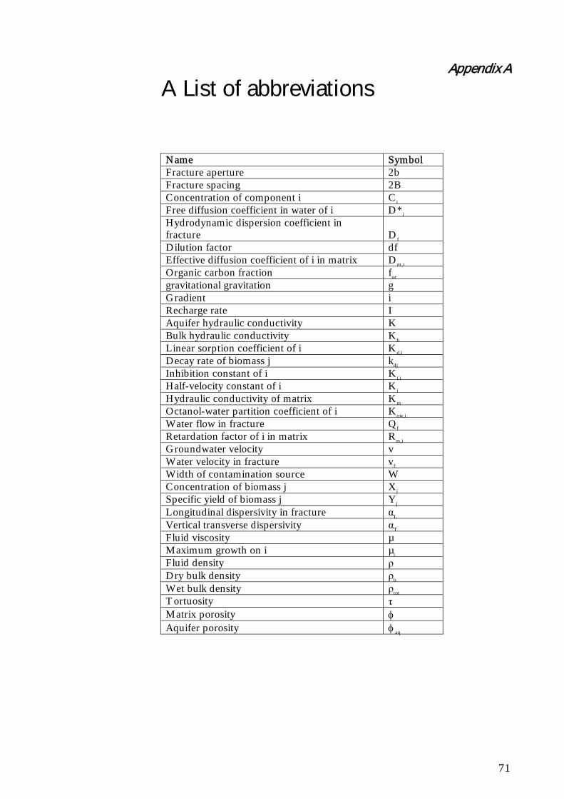
Appendix A

71

A List of abbreviations

Name Symbol Fracture aperture 2b Fracture spacing 2B Concentration of component i Ci Free diffusion coefficient in water of i D*i Hydrodynamic dispersion coefficient in fracture Df Dilution factor df Effective diffusion coefficient of i in matrix Dm,i Organic carbon fraction foc gravitational gravitation g Gradient i Recharge rate I Aquifer hydraulic conductivity K Bulk hydraulic conductivity Kb Linear sorption coefficient of i Kd,i Decay rate of biomass j kdj Inhibition constant of i Ki,i Half-velocity constant of i Ki Hydraulic conductivity of matrix Km Octanol-water partition coefficient of i Kow,i Water flow in fracture Qf Retardation factor of i in matrix Rm,i Groundwater velocity v Water velocity in fracture vf Width of contamination source W Concentration of biomass j Xj Specific yield of biomass j Yj Longitudinal dispersivity in fracture αL Vertical transverse dispersivity αT Fluid viscosity µ Maximum growth on i µi Fluid density ρ Dry bulk density ρb Wet bulk density ρtot Tortuosity τ Matrix porosity Aquifer porosity aq

Appendix B

73

B Processes and modeling of TCE sequential dechlorination

B.1 Kinetics models

It seems that researchers agree on the use of Monod or Michaelis-Menten equations to simulate reductive degradation of TCE and its daughter products. It was not possible to find differences in the two kinetics models used in the literature so they will be considered to be similar in the rest of the report. In these models, the degradation rate (mol.L-1.d-1) of the chlorinated ethenes has the following general form:

/i i

ii i

X Y Cr

C K

(B.1)

Where Ci is the concentration of the chlorinated ethene i (mol.L-1), µi is the maximum growth rate of i (d-1), X is the dechlorinating biomass concentration (cell.L-1), Y is the specific yield (cell.mol-1) and Ki is the half velocity coefficient of i (mol.L-1). As the degradation of the TCE corresponds to production of DCE, the change in chlorinated ethenes can be described with the following equation:

1i

i i

dCr r

dt (B.2)

Where ri is the degradation rate of the chlorinated ethene i and ri+1 is the production rate of chlorinated ethene I via the degradation of the higher chlorinated ethene.

74

Table B.1 - Reported values of kinetics parameters for dechlorination Kinetics coefficients

Units Symbol

Bagley 1998

Christ 2007

Chu 2004

Clapp 2004

Cupples 2004a Cupples 2004b Fennel

l 1998 Friis 2007

Garant 1998

Haston 1999

Lee 2004 Yu 2004

- Victoria, TX - - Bacteriu

m VS

VS mixed

VS highly enriched

KB-1/VC

Finellas

Mixed culture

KB-1TM - Victoria

, TX Victoria, TX PM EM

µPCE 0.006 0.316 0.277 2.395 - - - - - 0.264 - 0.128c

0.016c 3.001 0.08 0.074

µTCE 0.021 4.29 0.277 2.506 - 0.35 0.35 0.33 0.49 0.441 3.42 0.077c

0.013c 3.001 0.744 0.75

µDCE 0.015 0.563 - 0.766 0.4 0.46 - 0.44 0.43 0.441 0.16 0.048c

0.003c 0.394 0.132 0.083µ d-1

µVC 0.013 0.563 - 0.737 0.4 0.49 - 0.42 0.28 0.441 0.52 0.055c 0.003c 0.394 0.015 0.048

KPCE 0.06 0.2 1 0.88 - - - - - 0.54 - 70.7 0.11 0.2 3.86 1.63

KTCE 1.4 1.4 10 1.15 - 9 12.4 10 10 0.54 10b 17.4 1.4 0.05 2.76 1.8

KDCE 3.4 3.3 - 2.28 3.3 3.3 0.54 3.3b 11.9 3.3 3.3 1.9 1.76 K µmol.L-1

KVC 2.7 – 400 2.6 - 325 2.2 2.6 290 2.2b 3.83 2.6 2.6 602 62.6

Y mgbiomass.µmol-1 - 0.0027 0.017 0.006

1 0.0058 0.0082a 0.0083a 0.0031

a - - - 0.0082d 0.01e 0.01e

a calculated assuming 1.6*10-14g/cell [Cupples et al., 2003] b from [Haston and McCarty, 1999] c calculated assuming Y=8.2*10-3mgbiomass.�mol-1 d from [Cupples et al., 2003] e calculated assuming 0.6 g protein/g biomass [Cupples et al., 2003]

75

B.1.1 Competition between chlorinated ethenes

Some researchers have considered the competition between chlorinated ethenes for electron donors [Christ and Abriola, 2007, Chu et al., 2004, Cupples et al., 2004a, Cupples et al., 2004b, Garant and Lynd, 1998, Lee et al., 2004, Yu and Semprini, 2004 and Yu et al., 2005], among others. This competitive inhibition model is based on the assumption that a common catalyst is responsible for multiple dechlorination steps [Garant and Lynd, 1998]. Models accounting for this competition for electron donors are common in the recent literature, and it has been shown that it is possible to obtain a better fitting with a competitive than with a non-competitive model [Garant and Lynd, 1998 and Cupples et al., 2004a]. The general form for a competitive model, based on Monod kinetic is:

,

/

1

i ii

ji i

inh j

X Y Cr

CC K K

(B.3)

However the researchers do not agree on the types of competition, to be considered. In Chu et al. [2004], it has been shown that the dechlorination curves can have very different profiles depending on the inhibition considered in the model, therefore it is important to carefully consider which compounds are inhibitory in a system. Some researchers consider the competitive inhibition of all chlorinated ethenes at each dechlorination step [Cupples et al., 2004b and Garant and Lynd, 1998]. This means that TCE inhibits both DCE and VC dechlorination, DCE inhibits both TCE and VC degradation and VC inhibits both TCE and DCE degradation. Others considers that the inhibition constant of VC is very high compared to the half-velocity constant and is therefore not included in the model [Cupples et al., 2004b and Friis et al., 2007]. [Yu and Semprini, 2004 and Yu et al., 2005] suggest that the more chlorinated ethenes inhibit the degradation of the less chlorinated ethenes whereas the less chlorinated ethenes inhibit very weakly the dechlorination of the more chlorinated ethenes. The weak inhibition is therefore not included in the model. That means that TCE inhibits DCE and VC, and DCE inhibits only VC, whereas VC does not inhibit any degradation. Finally some studies consider different bacteria groups responsible for different dechlorination steps (this will be explained later), and in this case competitive inhibition occurs only between the chlorinated ethenes degraded by the same group [Lee et al., 2004]. The values of the inhibition coefficients are taken equal to the half-velocity constants in some studies [Garant and Lyng, 1998 Lee et al., 2004 Yu and Semprini, 2004 and Yu et al., 2005]. While in the others, it depends on the type of culture, used in the experiments (this will be detailed later). The reported values are presented in Table B.2.

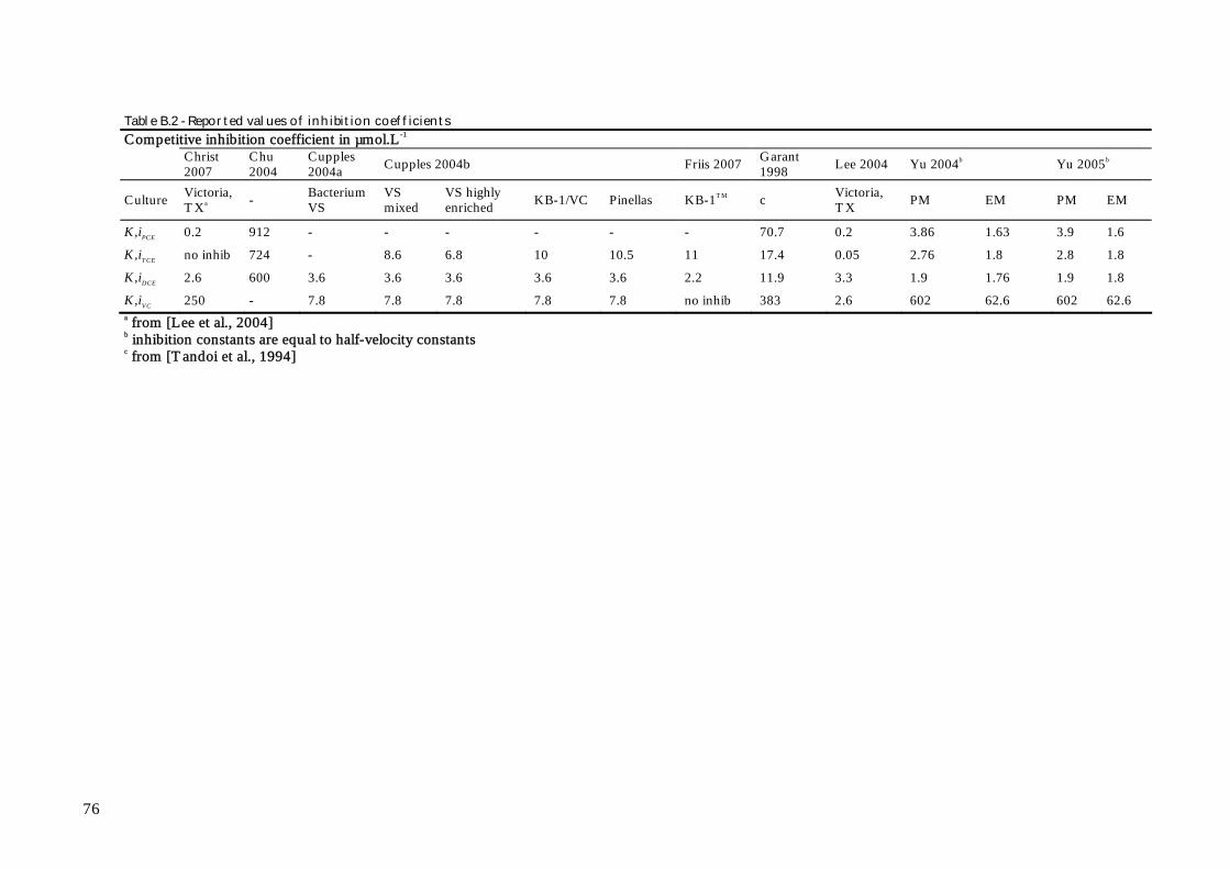
76

Table B.2 - Reported values of inhibition coefficients

Competitive inhibition coefficient in µmol.L-1

Christ 2007

Chu 2004

Cupples 2004a Cupples 2004b Friis 2007 Garant

1998 Lee 2004 Yu 2004b Yu 2005b

Culture Victoria, TXa

- Bacterium VS

VS mixed

VS highly enriched

KB-1/VC Pinellas KB-1TM c Victoria, TX

PM EM PM EM

K,iPCE 0.2 912 - - - - - - 70.7 0.2 3.86 1.63 3.9 1.6

K,iTCE no inhib 724 - 8.6 6.8 10 10.5 11 17.4 0.05 2.76 1.8 2.8 1.8

K,iDCE 2.6 600 3.6 3.6 3.6 3.6 3.6 2.2 11.9 3.3 1.9 1.76 1.9 1.8

K,iVC 250 - 7.8 7.8 7.8 7.8 7.8 no inhib 383 2.6 602 62.6 602 62.6 a from [Lee et al., 2004] b inhibition constants are equal to half-velocity constants c from [Tandoi et al., 1994]

77

B.1.2 Haldane inhibition

Haldane inhibition refers to the inhibition of a chlorinated compound on its own degradation rate. This phenomenon has been observed at high PCE and TCE concentrations [Yu and Semprini, 2004]. In this case, the inhibition term can be added in the equation, resulting in the following expression [Andrews, 1968]:

,,

/

1 1

i ii

i ji i

inh jhal i

X Y Cr

C CC K KK

(B.4)

Where Khal,i is the Haldane inhibition constant of chlorinated ethene i. In Yu and Semprini [2004], the model which takes into account Haldane inhibition (besides competitive inhibition) shows a better fit at high initial TCE concentration (around 4000 �M) than the competitive model only. The Haldane inhibition is applied to all chlorinated ethenes. The Haldane inhibition constants obtained from experimental data fittied with two different cultures are shown in Table B.3. Table B.3 - Haldane inhibition constants obtained by data fitting [Yu and Semprini, 2004]

Haldane inhibition coefficient in µmol.L-1

culture PM EV

K,halTCE 900 900

K,halDCE 6000 750

K,halVC 7000 750

B.1.3 Limiting substrate conditions

In some studies the electron donor is simulated to be rate-limiting in the dechlorination reactions [Bagley, 1998, Christ and Abiola, 2007, Chu et al., 2004, Cupples et al., 2004a, Fennel and Gossett, 1998, Lee et al., 2004 and Yang and McCarty, 1998]. In order to take into account the rate limitation by an electron donor, the degradation rate is modified as follow:

/i i ED

ii i ED ED

X Y C Cr

C K C K

(B.5)

Where CED is the electron donor (often hydrogen) concentration and KED is the electron donor half-velocity coefficient. Other studies report the existence of a threshold concentration, which reflects the concentration under which there is no further dechlorination [Smatlak and Gossett, 1996 and Yang and McCarty, 1998]. In this case, the degradation rate can be written, [Christ and Abiola, 2007, Cupples et al., 2004a, Fennel and Gossett, 1998, Lee et al., 2004]:

*

*

/i i ED EDi

i i ED ED ED

X Y C C Cr

C K C C K

(B.6)

78

Where C*

ED is the electron donor threshold concentration. In general, the values reported in literature refer to hydrogen as electron donor. These values can be found in Table B.4. Table B.4 - Reported values for hydrogen half-velocity coefficient and threshold concentration

Hydrogen half-velocity coefficient and threshold concentration in µmol.L-1

Bagley 1998

Christ 2007

Chu 2004

Clapp 2004

Cupples 2004a

Fennell 1998

Lee 2004

Smatlak 1996

Yang 1998

K,iPCE 0.009 – 0.1

K,iTCE 0.014 – 0.1

-

K,iDCE 0.021 – 0.1

K,iVC 0.017 – 0.1

0.1 10 0.075

0.007

0.5 0.5a 0.1 -

CH* - 0.002 - 0.0015

0.0009

<0.0015

0.002

<0.002 0.002

B.1.4 Biomass growth

Degrading of TCE and its daughter products results in the growth of the dechlorinating bacteria. Hence ,depending on the experiment’s duration, it may not be reasonable to assume a constant biomass concentration. Therefore numerous studies take into account biomass growth during dechlorination. In this case, the change in biomass over time is given by:

i di

dXY r k X

dt (B.7)

Where X is the dechlorinating biomass concentration (cell.L-1), ri is the degradation rate of the chlorinated ethene i (mol.L-1.d-1), Y is the specific yield (cell.mol-1) and kd is the decay constant of the dechlorinating microorganisms (d-1). The decay constant depends on the type of culture and the experiments/field conditions. The reported values are summarized in Table B.5.

79

Table B.5 - Reported values of decay rate in d-1

Christ 2007

Chu 2004 Clapp 2004 Cupples

2004a Cupples 2004b Fennell 1998

Friis 2007 Lee 2004 Yu 2004

Culture Victoria, TX - PCE-

DCE DCE-ETH

Bacterium VS

VS mixed

VS highly enriched

KB-1/VC Pinellas Mixed

cultureKB-1TM VictoriaTX PM EM

kd 0.05 0.03 0.01 0.003 0.05a 0.05a 0.024 0.05a 0.05 0.024b a from [Cupples et al., 2003] b from [Fennell and Gossett, 1998]

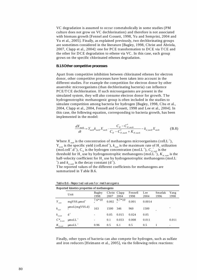
80

VC degradation is assumed to occur cometabolically in some studies (PM culture does not grow on VC dechlorination) and therefore is not associated with biomass growth [Fennel and Gossett, 1998, Yu and Semprini, 2004 and Yu et al., 2005]. Finally, as explained previously, two dechlorinating groups are sometimes considered in the literature [Bagley, 1998, Christ and Abriola, 2007, Clapp et al., 2004]: one for PCE transformation to DCE via TCE and the other for DCE degradation to ethene via VC. In this case, each group grows on the specific chlorinated ethenes degradation. B.1.5 Other competitive processes

Apart from competitive inhibition between chlorinated ethenes for electron donor, other competitive processes have been taken into account in the different studies. For example the competition for electron donor by other anaerobic microorganisms (than dechlorinating bacteria) can influence PCE/TCE dechlorination. If such microorganisms are present in the simulated system, they will also consume electron donor for growth. The hydrogenotrophic methanogenic group is often included in the studies to simulate competition among bacteria for hydrogen [Bagley, 1998, Chu et al., 2004, Clapp et al., 2004, Fennell and Gossett, 1998 and Lee et al., 2004]. In this case, the following equation, corresponding to bacteria growth, has been implemented in the model:

*

,,*

, ,

H H methmethmeth meth meth d meth meth

H H meth H meth

C CdXY k X k X

dt C C K

(B.8)

Where Xmeth is the concentration of methanogens microorganisms (cell.L-1), Ymeth is the specific yield (cell.mol-1), kmeth is the maximum rate of H2 utilization (mol.cell-1.d-1), CH is the hydrogen concentration (mol.L-1), CH

*

meth is the threshold for H2 use by hydrogenotrophic methanogens (mol.L-1), KH, meth is the half-velocity coefficient for H2 use by hydrogenotrophic methanogens (mol.L-

1) and kd, meth is the decay constant (d-1). The reported values of the different coefficients for methanogens are summarized in Table B.6. Table B.6 - Reported values for methanogens

Reported kinetics properties of methanogens

Unit Bagley 1998

Christ 2007

Clapp 2004

Fennell 1998

Lee 2004

Smatlak 1996

Yang 1998

Ymeth mgVSS.µmol-1 7.6*10-

4 0.002 9.7*10-

4 0.001 0.0014

kmeth µmol.(mgVSS.d)-

1 163 1500 346 960 1500

kd,meth d-1 - 0.05 0.015 0.024 0.05

-

C*H,meth µmol.L-1 - 0.1 0.033 0.008 0.011

-

0.011

KH,meth µmol.L-1 0.96 0.5 6.1 0.5 0.5 1 -

Finally, other types of bacteria can also compete for hydrogen, such as sulfate and iron reducers [Heimann et al., 2005], via the following redox reactions:

81

2

2 4 2

3 22

4 4

12

H SO H HS H O

Fe H Fe H

(B.9)

B.1.6 Fermentation process

The fermentation process, corresponding to the conversion of substrate into hydrogen, can be added in the model. Different substrates can be used to release hydrogen under anaerobic conditions, such as ethanol [Bagley, 1998 and Fennell and Gossett, 1998], pentanol [Christ and Abriola, 2007], butyric acid [Fennell and Gossett, 1998], propionic acid [Fennell and Gossett, 1998 and Yang and McCarty, 1998], lactic acid [Fennell and Gossett, 1998], glucose [Lee et al., 2004], benzoate [Yang and McCarty, 1998]. Examples of fermentation reactions are given below: Fermentation to acetate and H2 2 2butyrate 2 2 acetate 2H O H H (B.10)

2 2ethanol acetate 2H O H H (B.11)

2 3 2lactate 2 acetate 2H O HCO H H (B.12)

2 3 2propionate 3 acetate 3H O HCO H H (B.13)

2 3 2benzoate 7 3 acetate 3 3H O HCO H H (B.14) Fermentation to propionate and acetate

3 22 2 1 1ethanol propionate acetate3 3 3 3HCO H H O (B.15)

2 1 1 1lactate propionate acetate 33 3 3 3HCO H (B.16)

Glucose fermentation

2 2 3glucose 2 butyrate 2 2 3H O H HCO H (B.17)

2 2 3glucose 4 2acetate 4 2 4H O H HCO H (B.18)

2 3glucose 2 2ethanol 2 2H O HCO H (B.19) Depending on the primary substrate, the fermentation step is simulating using a combination of these equations. The rates of the different reactions are assumed to follow Monod kinetics. These reactions occur only when they are thermodynamically feasible (i.e when Gibbs free energy of the reaction is negative). This means that hydrogen concentration has to be low enough to allow fermentation to occur. The fermentation step is simulated in Fennell and Gossett [1998] with the following equation:

*

,

donor donor

s donor

k X S SdS

dt K S

(B.20)

Where kdonor is the maximum specific rate of donor degradation (mol.cell-1.d-1), Xdonor is the donor fermenting biomass concentration (cell.L-1), KS, donor is the half-velocity coefficient for the donor (mol.L-1), S is the donor concentration

82

(mol.L-1), S* is the hypothetical donor concentration that would result in ΔGrxn = ΔGcritical. The term S – S* allows the reaction only if it is thermodynamically feasible. However it was shown that substituting (S – S*) by S has a little impact on the results of the model in Fennell and Gossett [1998]. In the same way, the reaction rate in Christ and Abriola [2007] does not take S* into account. The amount of hydrogen (or acetate) produced during fermentation step can be calculated with the stoichoimetric coefficients of reactions (B.10) to (B.19). However it is difficult to relate hydrogen production directly to dechlorination because the produced hydrogen is consumed by different bacteria groups; and the dechlorinating biomass is only one of them. The growth of the fermenting biomass can also be taken into account, as well as the consumption of acetic acid by methanogens [Bagley, 1998].

Figure B.1- Schematic overview of anaerobic dechlorination and interaction with fermentative, reductive and methanogenic bacteria from [Jørgensen et al., 2005] B.1.7 Conclusion

Anaerobic dechlorination consists of many different processes which interact with each other to form a complex biochemical system, especially taking into consideration the fermentation step, which leads to hydrogen production. These different processes have been studied to various degrees in the literature and there is not any single paper, which takes into account this entire system, from dechlorination to redox condition and substrate fermentation. Typically some processes (such as electron donor limitation and fermentation mainly) are disregarded in order to simplify the model formulation.

Appendix C

83

C Results from treatability study experiments

The treatability study aimed to assess the potential for TCE dechlorination at a given field site. In these experiments perspective, groundwater and sediments from the site were mixed with TCE and concentrations of several compounds (TCE and its degradation products, redox compounds, electron donor) were measured under different conditions:

Unamended conditions Addition of electron donor Addition of both electron donor and dechlorinating culture

The experimental data used in this study comes from Rugårdsvej field site, where TCE/cis-DCE contamination is present in both sand and clay materials. Hence the treatability study has been performed with both sand and clay sediments in the experimental bottles [Jørgensen et al, 2007b]. Sand sediments are taken from three boreholes in the secondary groundwater magazine (samples K, L and M). Two electron donors are tested, lactate and propionate and the enriched culture KB-1TM is used for bioaugmentation.

Figure C.1 - TCE degradation in experiments with K sediment and lactate as electron donor – note that the time axis scale varies between figures

Figure C.2 - TCE degradation in experiments with K sediment and propionate as electron donor – note that the time axis scale varies between figures

84

Dechlorination is incomplete under natural conditions and that is necessary to add electron donor to degrade completely TCE completely to ethene. The addition of dechlorinating biomass accelerates the degradation processes. These results suggest the presence of two bacteria groups, one responsible for the dechlorination to cis-DCE and another (Dehalococcoides), which is able to degrade cis-DCE to ethene. In the natural conditions experiments, the first group degrades TCE to cis-DCE, but in the absence of substrate, the second group cannot grow and no further degradation is observed. In the experiment with electron donor addition, the initial small population of Dehalococcoides grows on the added substrate before being able to degrade cis-DCE and VC. The lag-time between TCE and cis-DCE degradation corresponds to the “growing time” of the second bacteria group. In the 11 and 7 K experiments, cis-DCE degradation occurs as soon as KB-1 culture is introduced (day 57), resulting in a faster dechlorination. The same experiments have been performed with clay sediments instead of sand from a groundwater aquifer. The clay material comes from three different locations (samples N, O and P) and 5 electron donors have been tested: lactate, propionate, HRC, Chitorem and Newmann zone. KB-1TM culture was added to the samples after 57 days.

Figure C.3 – TCE degradation with N sample (clay) and lactate (left) and propionate (right) as electron donor As it can be seen on Figure C.3, there is a release of cis-DCE from the clay sediments into the water sample, at the beginning of the experiments. This indicates that sorption processes occur in this system. The three experiments conditions represent the different remediation strategies that can be applied at a contaminated site:

Natural attenuation Biostimulation with injection of substrate Biostimualtion combined with bioaugmentation

The experimental data presented in this section have been used to conceptualize the dechlorination model and determine the kinetics parameters.

Appendix D

85

D Assessment of the different processes

D.1 Limiting substrate conditions

Limiting substrate conditions are of importance, as they decrease the degradation rate and slow down the dechlorination process. Substrate limiting conditions are particularly important when the chosen electron donor releases hydrogen slowly, as it is the case for propionate, for example. On the contrary, lactate is known to ferment relatively fast under anaerobic conditions [He et al., 2002]. Taking into account substrate limitation requires that the concentration of electron donor (i.e hydrogen in the case of anaerobic dechlorination) is known (see Section B.1.3). As explained previously, hydrogen is usually not injected directly at the field site, but is produced by fermentation of substrates of diverse types (lactate, propionate, ethanol…). Hence, in order to consider the substrate limiting conditions, the fermentation step must also be implemented in the model. Furthermore, hydrogen is consumed by different bacteria, besides the dechlorinating biomass, which usually includes sulfate/iron reducers, methanogens and acetogens (see Figure B.1). Finally, thermodynamics are also expected to play an important role in the concentration of hydrogen, notably during the fermentation step, and would need to be included in such a model. The implementation of these processes in the model entails an increase in the amount of parameters. As no prior information is usually available on the different bacteria populations present at a site, this also increases the uncertainty of the model. If the thermodynamics are disregarded then the model includes 16 variables (among them 7 bacteria populations) and 50 parameters, on most of which no prior information was available. Since the objective of this study and the further use of the model, it was decided to disregard the limiting substrate conditions in the degradation model.

D.2 Competitive inhibition between chlorinated ethenes

Most of the recent studies consider competitive inhibition between chlorinated ethenes, as their inclusion considerably improves the model accuracy. Hence it seems important to introduce this phenomenon in the model. Furthermore, the inhibition constants are assessed in several studies, so it is possible to find typical ranges for the kinetic parameters associated with this process.

D.3 Haldane inhibition

Haldane inhibition in TCE dechlorination has been reported in few studies and is a relevant process only for high concentrations (around 4000 µM [Yu and Semprini, 2004]). The concentrations from experimental data are very low compared to this value (maximum 50 µM). Hence Haldane inhibition is not relevant to simulate sequential degradation during the microcosm

86

experiments. However the concentration at contaminated sites can reach very high values and Haldane inhibition may become an important process in some cases. But in the absence of compatible microcosm experimental data to calibrate the Haldane constants, this process will be disregarded in this study.

D.4 Biomass growth/decay

Biomass is reported to grow by several orders of magnitude during TCE dechlorination experiments in several studies. As such a growth influences greatly the degradation rates, this process has to be included in the model. Modeling of biomass growth/decay can be simply implemented with Monod kinetics. Furthermore, the presence of two bacterial groups, as reported in other studies, seems to be an important aspect regarding the experimental data. Hence, one group will be assumed to grow only on TCE degradation, while a second one grows via cis-DCE and VC degradation.

Appendix E

87

E Sensitivity analysis

The sensitivity analysis is applied to a “base case”, and the change in the output concentrations, due to change in one parameter, is calculated. The “base case” parameters are chosen, in order to obtain output curves, close to the one obtained with experiments. The “base case” parameters are shown in Table E.1. It has to be noticed that a same specific yield value is assumed for both biomass groups. Furthermore, X10 and X20 are the initial biomass concentrations. While no prior information is available on the initial concentration of group 1, the initial concentration of group 2 can be estimated. Hence this group represents the concentration of Dehalococcoides, which has been added to the sample. Based on the estimated amount of Dehalococcoides cells in the KB-1 culture, and the dilution factor, it is possible to have an estimation for X20. However, this number is subject to uncertainty, that is why it is considered as a parameter to optimize. The base case is based on the experimental protocol followed during the treatability study. This means that the 2nd biomass group is assumed to be introduced first 57 days after the beginning of the experiment. Furthermore, the initial TCE concentration is set to 15 µM, as this value is close to the ones observed in experiments.

E.1 Estimation of X2o

A cell density of 108 cells/mL is commonly used for KB-1 culture [Dennis, pers. communation, 2008], of which a varying amount is Dehalococooides. During microcosm experiments, the culture is commonly diluted between 300 and 3000 times [Jørgensen et al., 2005], resulting in an initial concentration in Dehalococcoides between 107 – 4*108 cells/L. Table E.1 - Base case parameters

Units Base case

µTCE d-1 2

µDCE d-1 0.1

µVC d-1 0.1

KTCE µmol.L-1 10

KDCE µmol.L-1 3.3

KVC µmol.L-1 2.6

Ki,TCE µmol.L-1 10

Ki,DCE µmol.L-1 3.6

Ki,VC µmol.L-1 7.8

Y cell.µmol-1 5.2*108

kd1 d-1 0.03

kd2 d-1 0.03

X10 cell.L-1 8*104

X20 cell.L-1 2.5*108

88

Figure E.1 – Base case simulation results

E.2 Sensitivity assessment

The sensitivity is assessed by calculating the sensitivity index S, related to the variation of each parameter [Spitz and Moreno, 1996]:

idCS

dPP

(E.1)

Where |dCi|is the difference in concentration of compound i between the base case and sensitivity case, dP is the change in input parameter and P is the initial input parameter value. E.2.1 Parameter value range in literature

In Table E.2, the ranges found in the literature for the different parameters are shown. The ranges for some of the parameters are very wide, with several orders of magnitude. It has to be noticed that these parameters are reported for different cultures, electron donors and experimental conditions.

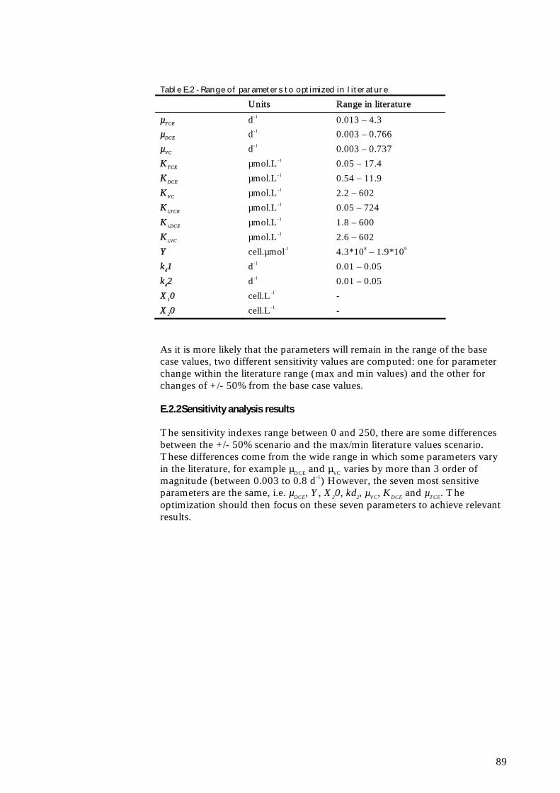
89

Table E.2 - Range of parameters to optimized in literature

Units Range in literature

µTCE d-1 0.013 – 4.3

µDCE d-1 0.003 – 0.766

µVC d-1 0.003 – 0.737

KTCE µmol.L-1 0.05 – 17.4

KDCE µmol.L-1 0.54 – 11.9

KVC µmol.L-1 2.2 – 602

Ki,TCE µmol.L-1 0.05 – 724

Ki,DCE µmol.L-1 1.8 – 600

Ki,VC µmol.L-1 2.6 – 602

Y cell.µmol-1 4.3*108 – 1.9*109

kd1 d-1 0.01 – 0.05

kd2 d-1 0.01 – 0.05

X10 cell.L-1 -

X20 cell.L-1 -

As it is more likely that the parameters will remain in the range of the base case values, two different sensitivity values are computed: one for parameter change within the literature range (max and min values) and the other for changes of +/- 50% from the base case values. E.2.2 Sensitivity analysis results

The sensitivity indexes range between 0 and 250, there are some differences between the +/- 50% scenario and the max/min literature values scenario. These differences come from the wide range in which some parameters vary in the literature, for example µDCE and µVC varies by more than 3 order of magnitude (between 0.003 to 0.8 d-1) However, the seven most sensitive parameters are the same, i.e. µDCE, Y, X20, kd2, µVC, KDCE and µTCE. The optimization should then focus on these seven parameters to achieve relevant results.

90

Table E.3 - Normalized sensitivity index for +/- 50% variation and literature extreme values

+/- 50% Max/min in literature

µDCE 161 163

Y 37 26

X20 37 61

kd2 34 35

µVC 32 143

KDCE 27 28

µTCE 24 226

KVC 17 10

Ki,DCE 16 12

KTCE 10 8

Ki,VC 8 8

X10 5 2

kd1 2 2

Ki,TCE 0 0

E.3 Experimental data from [Friis et al., 2007]

In these experiments, electron donor and KB-1 culture are added at the beginning of the experiments. Furthermore, there are no bacteria present in the bottle prior to the addition of KB-1. Hence, it is possible to estimate the different biomass populations, from the estimated cell density of KB-1 culture. In these experiments, the culture is diluted 300 times [Friis et al., 2007], leading to an initial Dehalococcoides concentration (X20) between 108 and 109 cells/L, and other biomass population (X10) approximately 2.3*108 to 2.3*109 cell/L. Among the seven parameters to optimize, it can be assumed that only the three maximum growth rates are different from one experiment set to the other (with different electron donor and/or temperature). Hence, it is expected that the four other parameters have a common optimized values, valid for all the experiments. The optimization script aims at reducing the root mean squared error (RMSE), as defined by:

2

sim measRMSE C C (E.2)

As explained previously, lactate is a fast hydrogen release, while propionate releases hydrogen much slower. Hence, it is expected that the experiments with lactate-amended culture correspond better to the no-limiting substrate assumption. Therefore it was decided to optimize all parameters with lactate-amended results and then to use the optimized values of KDCE, Y, X20 and kd2 for results with propionate, and optimize only the growth rates.

Appendix F

91

F Model verification – analytical solution

The numerical model is verified by comparing results to an analytical solution for a system of parallel fractures [Sudicky and Frind, 1982]. This analytical solution is also used in SprækkeJAGG [SprakkeJAGG, 2008] and gives the exact solution for concentration in the fracture and matrix at steady-state with a constant concentration at the fracture inlet. In this model, the transport in the matrix is assumed to be one-dimensional in the direction perpendicular to the matrix. Furthermore the degradation rate is assumed to be a 1st order. The parameters used in this verification are listed in Table F.1. Table F.1 - Parameters used for the model verification

Parameters Symbol Value Unit

Net recharge I 0.1 m/year

Fracture spacing 2B 0.2 m

Fracture aperture 2b 0.001 m

Water velocity in fracture vf 20 m/year

Matrix porosity 0.33 -

Longitudinal dispersivity in fracture L 0.1 m

Fracture dispersion coefficient Df 2 m2/year

Matrix diffusion coefficient Dm 0.0066 m2/year

Degradation rate 0.5 year-1

Start concentration C0 1400 mg/L

92

Concentration in mg/L0 200 400 600 800 1000 1200 1400

dep

th in

m

0

1

2

3

4

5

0 m (fracture)0.02 m0.05 m0.1 m

Figure F.1 – Contaminant concentration at different distances from the fracture for the numerical model (line) and analytical solution (symbol) for the parameters given in Table F.1

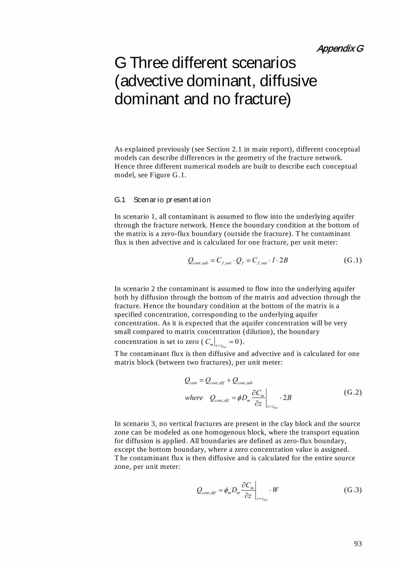
Appendix G

93

G Three different scenarios (advective dominant, diffusive dominant and no fracture)

As explained previously (see Section 2.1 in main report), different conceptual models can describe differences in the geometry of the fracture network. Hence three different numerical models are built to describe each conceptual model, see Figure G.1.

G.1 Scenario presentation

In scenario 1, all contaminant is assumed to flow into the underlying aquifer through the fracture network. Hence the boundary condition at the bottom of the matrix is a zero-flux boundary (outside the fracture). The contaminant flux is then advective and is calculated for one fracture, per unit meter: , , , 2cont adv f out f f outQ C Q C I B (G.1)

In scenario 2 the contaminant is assumed to flow into the underlying aquifer both by diffusion through the bottom of the matrix and advection through the fracture. Hence the boundary condition at the bottom of the matrix is a specified concentration, corresponding to the underlying aquifer concentration. As it is expected that the aquifer concentration will be very small compared to matrix concentration (dilution), the boundary concentration is set to zero ( 0

botm z z

C

).

The contaminant flux is then diffusive and advective and is calculated for one matrix block (between two fractures), per unit meter:

, ,

, 2bot

cont cont dif cont adv

mcont dif m

z z

Q Q Q

Cwhere Q D B

z

(G.2)

In scenario 3, no vertical fractures are present in the clay block and the source zone can be modeled as one homogenous block, where the transport equation for diffusion is applied. All boundaries are defined as zero-flux boundary, except the bottom boundary, where a zero concentration value is assigned. The contaminant flux is then diffusive and is calculated for the entire source zone, per unit meter:

,

bot

mcont dif m m

z z

CQ D W

z

(G.3)

94

Where W is the width of the source zone. Note that this is reasonable for large W, otherwise the diffusion is expected to occur in the three dimensions.

Figure G.1 – Illustration of the three transport scenarios

G.2 Assessment of relative importance of advective vs. diffusive flux

The importance of the advective and diffusive fluxes is assessed for different fracture aperture and spacing configurations. Fracture aperture ranges typically between 30 and 30000 µm, while fracture spacing ranges between 0.005 and 1 m [Christiansen and Wood, 2006]. Furthermore fracture porosity ranges between 10-2 and 10—4 [Parker et al., 1997]. Hence, the combinations resulting in porosity out of this range can be disregarded (in yellow in Table G.1) and this results in 16 different configurations of fracture aperture and spacing. Table G.1 - Fracture porosity for the fracture aperture and spacing configurations

Fracture porosity 2B in m 2b in µm

0.005 0.05 0.1 0.5 1

30 6*10-3 6*10-4 6*10-4 6*10-5 3*10-5

100 2*10-2 2*10-3 1*10-3 2*10-4 1*10-4

300 6*10-2 6*10-3 3*10-3 6*10-4 3*10-4

1500 3*10-1 3*10-2 1.5*10-2 3*10-3 1.5*10-3

3000 6*10-1 6*10-2 3*10-2 6*10-3 3*10-3

The different simulations are performed with an uniform initial concentration in the matrix and fracture Cm(x,z,t=0) = 100 mmol/m3 and assuming no degradation in the system: the contaminant is removed out of the matrix by the flushing of clean rain water in the fracture. It can be seen in Figure G.2 that the flux through the bottom of the matrix is not sensitive to variation of fracture aperture. On the contrary, Figure G.3 shows that the diffusive flux increases with reducing fracture spacing, from 9% for 2B = 1 m and up to 23% for 2B = 0.005 m. In these cases the recharge zone of one fracture is reduced (as the fracture spacing is small) and the water

Advectio

Diffusio

No fl

Advection

Diffusio

Diffusion Scenario 1 Scenario 2 Scenario 3

95

flow through the fracture, which is controlling the advective flux, is reduced, resulting in a larger diffusive flux. However the advective flux is the dominant flux in all configurations.

Fracture aperture (2b) in m1e-5 1e-4 1e-3 1e-2

% o

f di

ffus

ive

flux

thro

ugh

the

bott

om o

f th

e m

atrix

0

20

40

60

80

1002B = 0.005 m2B = 0.05 m2B = 0.1m2B = 0.5 m2B = 0.1 m

Figure G.2 – Percent of flux through matrix as a function of fracture aperture 2b

fracture spacing (2B) in m0,001 0,01 0,1 1

% o

f di

ffus

ive

flux

thro

ugh

the

bott

om o

f th

e m

atrix

0

20

40

60

80

1002b = 30 µm2b = 100 µm2b = 300 µm2b = 1.5 mm2b = 3 mm

Figure G.3 - Percent of flux through matrix as a function of fracture spacing 2B The influence of applying scenario 1 instead of scenario 2 for the configurations where a diffusive flux of above 10% has been assessed. The main objective of this single fracture model is to evaluate the output contaminant flux from the whole system, whether it comes from diffusion through the matrix or advection along fracture. Hence for a chosen configuration (2b = 10 µm and 2B = 0.05 m), where the diffusive flux represents more than 15% (see Figure G.3) scenario 1 (where there is no diffusion of contaminant through the bottom of the fracture) and scenario 2

96

are simulated by the numerical model. The outputs of the two models, in term of flux and contaminant distribution in the matrix, are compared. On Figure G.4, the different components (diffusive, advective and total) of the contaminant flux are plotted and it can be seen that the diffusive flux through the matrix represents more than 15% (red line). However comparing the total flux (green line) with the advective flux resulting from scenario 1 (Figure G.5), it can be seen that the two scenarios result in similar contaminant flux at the outlet of the system.

Time in years0 50 100 150 200

flux

in m

mo

l/ye

ar/

m

0,0

0,2

0,4

0,6

0,8

1,0flux through fractureflux through matrixTotal flux

Figure G.4 - Flux at the output of the system in scenario 2 (for 2b = 10-4 m and 2B = 0.05 m)

time in years0 50 100 150 200

flux

in m

mol

/yea

r/m

0,0

0,2

0,4

0,6

0,8

1,0Total flux for advective case (scenario 1)Total flux for advective/diffusive case (scenario 2)

Figure G.5 - Comparison of total flux out of the system for scenario 1 and 2 (for 2b = 10-4 m and 2B = 0.05 m) The contaminant distribution in the matrix at different times is shown on Figure G.6. The contaminant distributions are very similar for the two cases,

97

except the presence of a concentration gradient at the bottom of the matrix in scenario 2.

Figure G.6 - Contaminant distribution in the matrix for different times, in case of advection only (left) and (advection and diffusion through bottom of matrix (right) Disregarding the presence of a diffusive flux through the bottom of the matrix, which can represent between 9 and 25 % of the total flux, does not seem to change the model results, in terms of the total contaminant flux at the outlet and the contaminant distribution in the matrix. Therefore, it was decided to use only scenario 1, for clay systems presenting vertical fractures and scenario 3 for clay system without vertical fractures.

Appendix H

99

H Impact of the choice of initial condition

The initial condition in the matrix should correspond to the state of the system at the end of the contamination phase. As the duration and characteristics of this contamination phase are often not known precisely, the initial condition of the system must be based on field measurements or even assumed. Therefore it is important to assess the sensitivity of the numerical model to different initial concentration distributions. Three different scenarios will be assessed:

- Homogenous initial concentration in the entire matrix ( 0( , , 0)mC x z t C )

- Simulation of a 30-years contamination phase with constant concentration at the top of the matrix

- Simulation of a 30-years contamination phase with a constant concentration at the inlet of the fracture

As it is expected that the initial condition scenario will be most significant for geometric configurations with a large fracture spacing, the simulations were conducted with 2b = 3mm and 2B = 1 m. In order to be able to compare the different initial conditions on the output of the system (mass removal and contaminant flux), the same initial total mass of contaminant has been used, Mtot,ini = 532 mmol = 70 g. It can be seen on Figure H.1 that these scenarios give very different initial concentration distributions. Figure H.2 and Figure H.3 show these different configurations give similar results with regards to both timing and marginally mass removal efficiency. Results show that the mass removal time is decreasing from scenario A to scenario C. In scenario B and C most of the contamination is close to the fracture; therefore the diffusion time from the matrix to the fracture is smaller than in scenario A.

100

Figure H.1 - Initial concentration distributions for the three initial conditions

time in years0 200 400 600 800 1000

Tot

al m

ass

in s

yste

m in

mm

ol

0

100

200

300

400

500

600Homogenous initial concentration30-years contamination with constant concentration at the top of the matrix30-years contamination with a constant concentration at the inlet of the fracture

Figure H.2 - Total mass remaining in the system for the three initial conditions

101

time in years0 200 400 600 800 1000

Aqu

eous

con

cen

tra

tion

in m

mo

l/m3

0

20

40

60

80

100

120

140

160

180

200Homogenous initial concentration30-years contamination with a constant concentration at the top of the matrix30-years contamination with a constant concentration at the inlet of the fracture

Figure H.3 – Concentration at the fracture outlet for the three initial conditions The use of different initial conditions can lead to different results, notably concerning the mass removal efficiency. However, as results are fairly similar the homogenous initial condition (A) will be used in the following sections of the report.

Appendix I

103

I Different degradation scenarios

As explained in Section 4.3.4 in the main report, the results from field samples and literature studies have shown dechlorination may occur in a reaction zone near the high permeable sand zone (fractures), but no biomass transport or growth is expected deep within the clay matrix. Hence different scenarios need to be considered relative to degradation location:

- No degradation occurs in the system - Degradation occurs only in the high permeable zone, i.e. the fractures - A reaction zone is formed at the clay – fracture interface, where

degradation is also taking place - Degradation in the whole matrix

The last scenario is not likely to be realistic but isused to assess a “best case” case relative to degradation. In the absence of literature data, the degradation zone is assumed to be extended up to 0.05 m inside the clay matrix, corresponding to observations at Rugårdsvej field site. However the biomass growth in this reaction zone is restricted by pore size limitations [Lima and Sleep, 2007] and cannot be simulated in the same way as the biomass growth in the fracture. For the simplicity of the model, the biomass will be assumed to be constant both in the fracture and matrix, with a concentration of 108 cells/L [Miljøstyrelsen, 2008]. These four scenarios are applied to the base case configuration with the transport parameters in Section 5.2.2 in the main report, while the parameters relative to chlorinated solvents dechlorination are taken from optimization results in Section 3.4.1 in the main report. Finally a homogenous initial TCE concentration of 100 mmol/m3 is applied.

time in years0 50 100 150 200 250 300

Tot

al c

ont

amin

ant

ma

ss in

sys

tem

in m

mo

l

0

20

40

60

80

100

120

140


Figure I.1 - Remaining total contaminant mass in the system for the four degradation scenarios

104

time in years0 50 100 150 200 250 300

aque

ous

conc

entr

atio

n in

mm

ol/m

3

0

20

40

60

80


Figure I.2 –TCE concentration at the fracture outlet for the three degradation scenarios The scenario with degradation in the fracture only does not differ much from the scenario without degradation, especially concerning the mass removal rate in the system. This is due to the fact that the contaminant downward transport in the fracture, controlled by the groundwater velocity, is much higher than the degradation rate. Therefore the contaminant has no time to be degraded once it has reached the fracture (from counter diffusion from the matrix) and the production of daughter products (DCE and VC) is very limited (see Figure I.3). On the contrary in the presence of a reaction zone at the matrix – fracture interface, daughter products are formed (Figure I.3) and the mass removal occurs significantly faster (Figure I.1). As expected, under the assumption of degradation in the whole matrix, the mass removal is much faster.

degradation in fract and reaction zone in matrix

time in years50 100 150 200 250

0

20

40

60

80

100

degradation in fracture only

time in years50 100 150 200 250

Aqu

eou

s co

nce

ntra

tion

in m

mol

/m3

0

20

40

60

80

100TCE - no degrTCEDCEVC

degradation in fract and in the whole matrix

time in years50 100 150 200 250

0

20

40

60

80

100

Figure I.3 – TCE, DCE and VC concentrations at the fracture outlet for the three degradation scenarios (compared with TCE for the case without degradation)

Appendix J

105

J Sensitivity analysis

J.1 Sensitivity to fracture aperture and spacing

The model response to change in fracture aperture and spacing is assessed for the three different degradation scenarios by analyzing the output parameters shown on Figure J.1: time to remove 90% of the initial total contaminant mass, average time for the fracture outlet concentration to be lower than a limit concentration and finally average peak concentrations for the two daughter products. The different geometric configurations of Table G.1 are used with the transport and degradation parameters from the base case scenario.

Figure J.1 - Parameters for sensitivity analysis of fracture aperture and spacing – total mass on right axis (blue line) Clim is defined for each of the chlorinated compounds as a function of the groundwater quality standard (Cstandard) recommended in Miljøstyrelsen [2005] and an assumed dilution factor of 10 between the concentration at the fracture outlet and the resulting concentration in the underlying aquifer. Hence Clim = Cstandard*10. The dilution factor of 10 is assumed here, but does not change the main conclusions from this part.

time in years0 20 40 60 80 100 120 140

Aqu

eous

co

ncen

tra

tion

in m

mo

l/m3

0

20

40

60

80

100

Tot

al c

onta

min

ant

mas

s in

the

sys

tem

in m

mol

0

20

40

60

80

100

120

140

160TCEDCEVCtotal mass

Max concentration of

daughter

Time to remove 90% of the initial

Time to reach Ci < Clim

106

Table J.1 - Groundwater quality standard and output parameters from model

Cstandard Clim

µg/L µg/L µmol/L

TCE 1 10 0.08

cis-DCE 1 10 0.10

VC 0.2 2 0.03

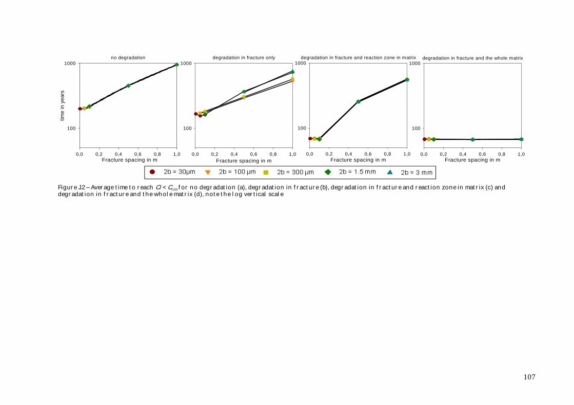
107

no degradation

0,0 0,2 0,4 0,6 0,8 1,0

time

in y

ea

rs

100

1000degradation in fracture only

Fracture spacing in m0,0 0,2 0,4 0,6 0,8 1,0

100

1000

0,0 0,2 0,4 0,6 0,8 1,0

100

1000

Fracture spacing in mFracture spacing in m

degradation in fracture and reaction zone in matrix

0,0 0,2 0,4 0,6 0,8 1,0

100

1000degradation in fracture and the whole matrix

Fracture spacing in m

Figure J.2 – Average time to reach Ci < Clim for no degradation (a), degradation in fracture (b), degradation in fracture and reaction zone in matrix (c) and degradation in fracture and the whole matrix (d), note the log vertical scale

108


0,0 0,2 0,4 0,6 0,8 1,0

time

in y

ears

10

100

1000

Fracture spacing in m0,0 0,2 0,4 0,6 0,8 1,0

10

100

1000


0,2 0,4 0,6 0,8 1,010

100

1000no degradation degradation in fracture only degradation in fracture and reaction zone in m atrix degradation in fracture and the whole m atrix


0,2 0,4 0,6 0,8 1,010

100

1000

Figure J.3– Average time to remove 90% of the initial contaminant mass, for no degradation (a), degradation in fracture (b), degradation in fracture and reaction zone in matrix (c) and degradation in fracture and the whole matrix (d), note the log vertical scale

fracture spacing in m

0,01 0,1 110

100


0,01 0,1 1

Aqu

eou

s co

nce

ntra

tion

in m

mol

/m3

0 ,1

1

10

100

degradation in fracture only degradation in fracture and reaction zone in m atrix degradation in fracture and the whole m atrix


0,01 0,1 110

100

Figure J.4 - Average maximum concentration for the daughter products (DCE and VC), for degradation in fracture (a), degradation in fracture and reaction zone in matrix (b) and degradation in fracture and the whole matrix (c), note the log vertical and horizontal scale

109

The single fracture/matrix model is not sensitive to the fracture aperture, except for the maximum daughter products concentration in case of degradation in fracture (Figure J.4 (a)) and a limited sensitivity for the average time to reach an output concentration below Clim in case of degradation in the fracture (Figure J.2 (b)). In these two cases, aperture reduction results in a higher water velocity in the fracture and therefore the daughter products do not have the time to be produced. Otherwise the non-sensitivity of this parameter is explained by the definition of flow in the fracture, which depends on the fracture spacing only (see Section 5.1.2 in the main report). On the contrary the model results are very sensitive to the fracture spacing: the mass removal time increases with fracture spacing, as well as the time to reach an output concentration below Clim. Furthermore, assuming degradation in the whole matrix leads to a decrease of the clean-up times. In this case, the model is less sensitive to fracture spacing.

J.2 Global sensitivity analysis

The sensitivity analysis is performed on all independent parameters (Table J.2), of which the value is changed by +/- 20%. The resulting change in the three output parameters (time to remove 90% of the initial contaminant mass, average time to reach Ci < Clim and average peak concentration of daughter products) is normalized to calculate the sensitivity index (see Appendix D). The sensitivity analysis is performed on the third degradation scenario (degradation in the fracture and in a reaction zone in the matrix) with a homogenous TCE concentration as initial condition. In order to be able to compare the different simulations, this initial concentration is corrected in order to maintain the same initial total mass. Table J.2 - Independent parameters for sensitivity analysis (in orange transport parameters, in green degradation parameters)

Parameter Symbol Value – base Unit Net recharge I 0.1 m/year Fracture spacing 2B 0.3 m Fracture aperture 2b 7*10-4 m Sorption coefficient TCE Kd_TCE 1 L/kg Sorption coefficient DCE Kd_DCE 0.7 L/kg Sorption coefficient VC Kd_VC 0.3 L/kg Matrix porosity 0.33 - Exponent p p 1 - Longitudinal dispersivity in f

αL 0.1 m Max growth rate TCE µTCE 730 year-1 Max growth rate DCE µDCE 138.7 year-1 Max growth rate VC µVC 51.1 year-1 Specific yield Y 5.2*108 cell.µmol-

1

Initial biomass XO 108 cell.L-1 Half velocity coefficient DCE KDCE 9.9 µmol.L-1

110

The four most sensitive independent parameters are the same for the different output considered, matrix porosity, fracture spacing, net recharge and TCE sorption coefficient. The most sensitive parameters are then the ones controlling transport, especially diffusion/sorption processes, and not dechlorination. The limiting process in this system is the counter diffusion out of the matrix, which is controlled by sorption, flushing of the fracture and fracture spacing. The two least sensitive parameters are the fracture aperture and longitudinal dispersivity in the fracture. The low sensitivity of this last parameter is due to the fact that transport in the fracture is mainly advective and not dispersive. Table J.3 - Sensitivity index for the three output parameters

Parameter M< 10%Mini

Parameter Ci < Clim Parameter max

Ci

Matrix porosity 55.0 Matrix porosity 115.0 Fracture spacing 31.0

Net recharge 52.5 Fracture spacing 95.0 Matrix porosity 24.8

Fracture spacing 42.5 Sorption coefficient TCE 61.7 Net recharge 21.9

Sorption coefficient TCE 35.0 Net recharge 58.3 Sorption coefficient

TCE 18.7

Sorption coefficient DCE 20.0 Specific yield 47.5 Max growth rate TCE 17.6

Specific yield 20.0 Initial biomass 47.5 Initial biomass 16.3

Initial biomass 20.0 Sorption coefficient DCE 34.2 Specific yield 16.1

Exponent p 10.0 Max growth rate DCE 22.5 Sorption coefficient DCE 14.8

Max growth rate DCE 10.0 Exponent p 20.0 Exponent p 6.3

Half velocity coefficient DCE 7.5 Max growth rate TCE 16.7 Max growth rate VC 5.2

Sorption coefficient VC 5.0 Half velocity

coefficient DCE 16.7 Max growth rate DCE 3.9

Max growth rate TCE 5.0 Max growth rate VC 7.5 Half velocity coefficient DCE 2.1

Max growth rate VC 5.0 Sorption coefficient VC 3.3

Sorption coefficient VC 2.0

Fracture aperture 0.0 Fracture aperture 1.7 Longitudinal dispersivity in fracture 1.6

Longitudinal dispersivity in fracture 0.0 Longitudinal

dispersivity in fracture 0.8 Fracture aperture 0.3

Sensitivity analysis has also been performed by varying the parameters in the typical ranges found in the literature and the same conclusions can be done, concerning the most and least sensitive parameters.

Appendix K

111

K Aquifer model - Sensitivity analysis

Numerous independent parameters are used in this model, but it is possible to group some parameters in order to reduce the amount of independent variables. For the case with top recharge, it appears that the dilution factor df depends on the flow factor (ff), defined as the ratio of the recharge rate I and the mean specific discharge (=K*i). The variable ff groups recharge rate I, hydraulic conductivity K and hydraulic gradient i. This concept is illustrated with some examples, where the aquifer thickness, the transverse vertical dispersivity, the porosity and the source width are fixed (b = 5m, T = 0.005 m, aq = 0.3 and W = 30m) while the hydraulic gradient, the recharge rate and hydraulic conductivity vary in order to keep ff = 0.5% (Table K.1 and Figure K.1). Table K.1 - Four scenarios with ff = 0.5%

Hydraulic conductivity Recharge rate

Hydraulic gradient

Flow factor

K I i ff m/year m/year - %

Scenario 1 2500 0.1 0.008 0.5 Scenario 2 5000 0.05 0.002 0.5 Scenario 3 10000 0.2 0.004 0.5 Scenario 4 30000 0.3 0.002 0.5

Caq/Cf,out in %0 2 4 6 8 10

dep

th in

m

-5

-4

-3

-2

-1

0

Scenario 1Scenario 2Scenario 3Scenario 4

Figure K.1 – Dilution factor for leaky aquifer along the cross section at 100 m from the source for the 4 scenarios The results are identical for all cases shown in Figure K.1. For the confined aquifer case, df depends on the mean specific discharge (=K*i), as shown with three examples on Figure K.2, with the same parameters and a mean

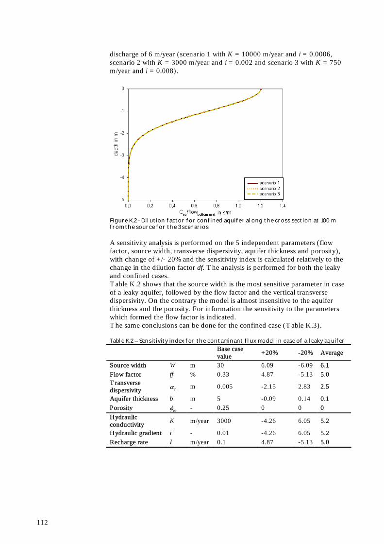
112

discharge of 6 m/year (scenario 1 with K = 10000 m/year and i = 0.0006, scenario 2 with K = 3000 m/year and i = 0.002 and scenario 3 with K = 750 m/year and i = 0.008).

Figure K.2 - Dilution factor for confined aquifer along the cross section at 100 m from the source for the 3 scenarios A sensitivity analysis is performed on the 5 independent parameters (flow factor, source width, transverse dispersivity, aquifer thickness and porosity), with change of +/- 20% and the sensitivity index is calculated relatively to the change in the dilution factor df. The analysis is performed for both the leaky and confined cases. Table K.2 shows that the source width is the most sensitive parameter in case of a leaky aquifer, followed by the flow factor and the vertical transverse dispersivity. On the contrary the model is almost insensitive to the aquifer thickness and the porosity. For information the sensitivity to the parameters which formed the flow factor is indicated. The same conclusions can be done for the confined case (Table K.3). Table K.2 – Sensitivity index for the contaminant flux model in case of a leaky aquifer

Base case value

+20% -20% Average

Source width W m 30 6.09 -6.09 6.1 Flow factor ff % 0.33 4.87 -5.13 5.0 Transverse dispersivity T m 0.005 -2.15 2.83 2.5

Aquifer thickness b m 5 -0.09 0.14 0.1 Porosity aq - 0.25 0 0 0 Hydraulic conductivity

K m/year 3000 -4.26 6.05 5.2

Hydraulic gradient i - 0.01 -4.26 6.05 5.2 Recharge rate I m/year 0.1 4.87 -5.13 5.0

113

Table K.3 - Sensitivity index for the contaminant flux model in case of a confined aquifer

Base case value +20% -20% Average

Flow factor ff m/s 30 -0.67 1 0.84 Source width W m 30 0.8 -0.81 0.81 Transverse dispersivity T m 0.005 -0.35 0.48 0.42

Aquifer thickness b m 5 0 0 0 Porosity aq - 0.25 0 0 0 Hydraulic conductivity

K m/year 3000 -0.67 1 0.84

Hydraulic gradient i - 0.01 -0.67 1 0.84

Model assessment of reductive dechlorination as a ...

Documents

Transcript of Model assessment of reductive dechlorination as a ...