Western UniversityScholarship@Western

Electronic Thesis and Dissertation Repository

August 2013

Reliability Models Applied to SmartphoneApplicationsSonia MeskiniThe University of Western Ontario

SupervisorLuiz Fernando CapretzThe University of Western Ontario

Graduate Program in Electrical and Computer Engineering

A thesis submitted in partial fulfillment of the requirements for the degree in Master of Engineering Science

© Sonia Meskini 2013

Follow this and additional works at: https://ir.lib.uwo.ca/etd

Part of the Other Computer Engineering Commons, Other Electrical and Computer EngineeringCommons, and the Software Engineering Commons

This Dissertation/Thesis is brought to you for free and open access by Scholarship@Western. It has been accepted for inclusion in Electronic Thesisand Dissertation Repository by an authorized administrator of Scholarship@Western. For more information, please contact tadam@uwo.ca,wlswadmin@uwo.ca.

Recommended CitationMeskini, Sonia, "Reliability Models Applied to Smartphone Applications" (2013). Electronic Thesis and Dissertation Repository. 1487.https://ir.lib.uwo.ca/etd/1487

Reliability Models Applied to Smartphone Applications

by

Sonia Meskini

Graduate Program: Electrical and Computer Engineering Department of Engineering Science

A thesis submitted in partial fulfillment of the requirements for the degree of

Master of Engineering Science

The School of Graduate and Postdoctoral Studies The University of Western Ontario

London, Ontario, Canada

© Sonia Meskini, 2013

ii

Abstract

Smartphones have become the most used electronic devices. They carry out most of the

functionalities of desktops, offering various useful applications that suit the user’s needs.

Therefore, instead of the operator, the user has been the main controller of the device and its

applications, therefore its reliability has become an emergent requirement. As a first step,

based on collected smartphone applications failure data, we investigated and evaluated the

efficacy of Software Reliability Growth Models (SRGMs) when applied to these smartphone

data in order to check whether they achieve the same accuracy as in the desktop/laptop area.

None of the selected models were able to account for the smartphone data satisfactorily.

Their failure is traced back to: (i) the hardware and software differences between desktops

and smartphones, (ii) the specific features of mobile applications compared to desktop

applications, and (iii) the different operational conditions and usage profiles. Thus, a

reliability model suited to smartphone applications is still needed. In the second step, we

applied the Weibull and Gamma distributions, and their two particular cases, Rayleigh and S-

Shaped, to model the smartphone failure data sorted by application version number and

grouped into different time periods. An estimation of the expected number of defects in each

application version was obtained. The performances of the distributions were then compared

amongst each other. We found that both Weibull and Gamma distributions can fit the failure

data of mobile applications, although the Gamma distribution is frequently more suited.

Keywords : Smartphone Applications, Software Reliability, Gamma Distribution,

Weibull Distribution, Rayleigh, S-Shaped, NHPP, Musa-Basic, Musa-Logarithmic.

iii

Dedicated to

My dearest father, Noureddine

My lovely mother, Habiba

They have been the biggest motivator and inspiration in my life.

iv

Acknowledgments

First of all I would like to thank my supervisor, Dr. Luiz Fernando Capretz, for his constant

guidance and assistance throughout this work and for being at the origin of my graduate

studies in this beautiful country. He was very helpful and encouraging in choosing the topic

of this thesis.

I also thank Dr. Keivan Kian-Mehr for his precious help in the initial stage of this work and

for orienting me in the wide field of Software Reliability Engineering.

I wish to express my sincere gratitude to Dr. Ali Bou Nassif for his moral and scientific

support. I have greatly benefited from his research methodology and his insightful scientific

approaches.

Many thanks go to a friend for providing me the failure data of the private Windows phone

application.

I would also like to thank my dissertation committee members and all the faculty members

and staff of the Department of Electrical and Computer Engineering for making my stay here

highly enjoyable.

My sincere thanks are dedicated to the Tunisian Ministry of Higher Education and Scientific

Research and for MUTAN, its representative body in Canada, for providing my Master’s

scholarship.

Finally, I would like to express my sincere thanks to my parents and my family for their

continuous help and encouragement.

v

Table of Contents

Acknowledgments.............................................................................................................. iv

Table of Contents ................................................................................................................ v

List of Tables ..................................................................................................................... ix

List of Figures ..................................................................................................................... x

Chapter 1 ............................................................................................................................. 1

1 Introduction .................................................................................................................... 1

1.1 Motivation and Research Questions ....................................................................... 2

1.2 Methodology ........................................................................................................... 3

1.3 Thesis Contributions ............................................................................................... 4

1.4 Thesis Outline ......................................................................................................... 5

Chapter 2 ............................................................................................................................. 7

2 Reliability Issue in the Mobile Area .............................................................................. 7

2.1 Rapid Development of Mobile Phones ................................................................... 7

2.2 Smartphone Versus Desktop/Laptop: the Hardware Difference ............................ 8

2.3 Smartphone Versus Desktop/Laptop: the Software Difference .............................. 8

2.4 Smartphone Versus Desktop/Laptop: the Operational Profile Difference ............. 9

2.5 Reliability of Smartphone Applications .................................................................. 9

2.5.1 Maintenance and Updates of Released Applications ................................ 10

2.5.2 Smartphone Applications Reliability ........................................................ 10

2.5.3 Smartphone Operating System Reliability................................................ 14

2.6 Summary ............................................................................................................... 17

Chapter 3 ........................................................................................................................... 18

3 Software Reliability Growth Models: A Road Map .................................................... 18

3.1 Mathematical Software Reliability Modeling ....................................................... 18

vi

3.2 Reliability Concepts .............................................................................................. 19

3.2.1 Non-Repairable Systems ........................................................................... 19

3.2.2 Repairable Systems ................................................................................... 21

3.3 Three Most Used Software Reliability Growth Models ....................................... 22

3.3.1 The NHPP Crow-AMSAA Model ............................................................ 23

3.3.2 Musa’s Basic Execution Time Model ....................................................... 26

3.3.3 Musa-Okumoto Logarithmic Poisson Model............................................ 28

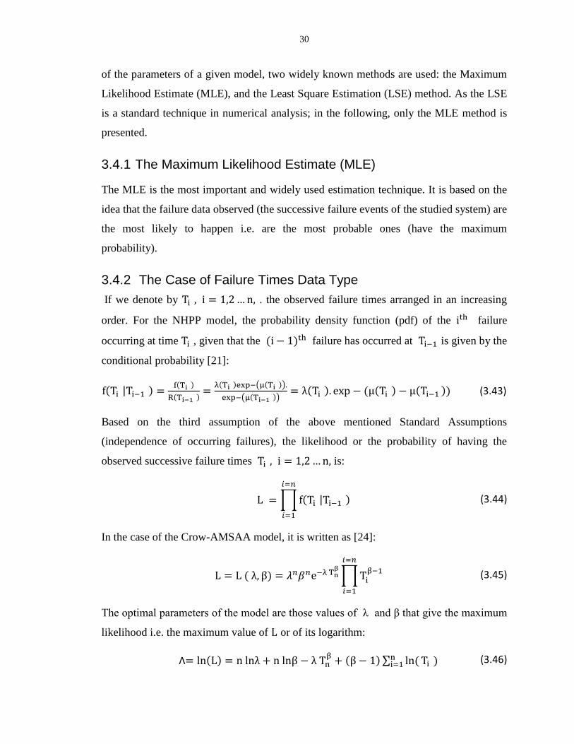
3.4 Parameters Estimation .......................................................................................... 29

3.4.1 The Maximum Likelihood Estimate (MLE) ............................................. 30

3.4.2 The Case of Failure Times Data Type ...................................................... 30

3.4.3 The Case of Grouped Data Type .............................................................. 31

3.5 Goodness-of-Fit Tests ........................................................................................... 32

3.5.1 The Cramer- Von Mises Goodness-of- Fit Test ....................................... 32

3.5.2 The Chi-Squared Goodness-of-Fit Test .................................................... 32

3.6 Summary ............................................................................................................... 33

Chapter 4 ........................................................................................................................... 34

4 Smartphone Failure Data and Application of SRGMs ................................................. 34

4.1 Data Collection ..................................................................................................... 34

4.2 Application of SRGMs to the Failure Data........................................................... 37

4.2.1 Choice of the Reliability Models .............................................................. 37

4.2.2 Experiments .............................................................................................. 38

4.2.3 Results ....................................................................................................... 40

4.3 Evaluation ............................................................................................................. 52

4.3.1 Operational Environments and Usage Profiles of Smartphone Applications

................................................................................................................... 52

4.3.2 Hardware and Software Limitations ......................................................... 53

vii

4.3.3 The Need to Reexamine the Standard Assumptions ................................. 54

4.4 Summary ............................................................................................................... 55

Chapter 5 ........................................................................................................................... 57

5 Failure Data Analysis of Smartphone Applications Using the Weibull and Gamma

Distributions ................................................................................................................. 57

5.1 Experiments .......................................................................................................... 57

5.2 The Weibull Distribution ...................................................................................... 58

5.3 The Gamma Distribution ...................................................................................... 60

5.4 Evaluation Criteria ................................................................................................ 61

5.5 Results ................................................................................................................... 62

5.5.1 Skype Application ..................................................................................... 62

5.5.2 Vtok Application ....................................................................................... 69

5.5.3 Windows Phone Application .................................................................... 72

5.6 Discussion ............................................................................................................. 75

5.7 Threats to Validity: ............................................................................................... 80

5.8 Summary ............................................................................................................... 81

Chapter 6 ........................................................................................................................... 83

6 Conclusions .................................................................................................................. 83

6.1 Conclusions and Perspectives ............................................................................... 83

6.2 Future Work .......................................................................................................... 85

Appendix A: Collected Failure Data for Skype, Vtok, and Windows Phone Applications

...................................................................................................................................... 91

Failure Data of the Skype Application.............................................................................. 91

Failure Data of the Vtok Application................................................................................ 92

Failure Data of the Windows Phone Application ............................................................. 94

The Dataset Grouped Per Version .................................................................................... 99

a) Skype ....................................................................................................................... 99

viii

b) Vtok ......................................................................................................................... 99

Appendix B: Source Code of the JAVA Program - Extracting the Needed Information

from the Crash File..................................................................................................... 100

Curriculum Vitae ............................................................................................................ 102

ix

List of Tables

Table 4-1 : Possible causes of applications crash ................................................................... 54

Table 5-1: Skype Version 1 - Error evaluation and model comparison ................................. 63

Table 5-2: Skype Version 2 - Error evaluation and model comparison ................................. 65

Table 5-3: Skype Version 3 - Error evaluation and model comparison ................................. 67

Table 5-4: Vtok Version 1 - Error evaluation and model comparison ................................... 69

Table 5-5: Vtok Version 2 - Error evaluation and model comparison ................................... 71

Table 5-6: Windows phone application (per weeks) - Error evaluation and model comparison

................................................................................................................................................. 73

Table 5-7: Windows phone application (per months) - Error evaluation and model

comparison .............................................................................................................................. 75

Table 5-8: Skype - The parameter values of the model distributions ..................................... 78

Table 5-9 : Vtok - The parameter values of the model distributions ...................................... 79

Table 5-10: Windows phone application - Parameter values of the model distributions ....... 80

x

List of Figures

Figure 2-1 : Malfunction rates for various smartphone models .............................................. 12

Figure 2-2 : Reliability of portable electronic devices ............................................................ 13

Figure 2-3 : Compared mobile operating systems reliability.................................................. 14

Figure 2-4 : Compared mobile operating systems shares ....................................................... 15

Figure 2-5 : Expected Smartphone user share, by OS ............................................................ 16

Figure 3-1: Use of a chosen SRGM to study the reliability of an application ........................ 29

Figure 4-1: Apple crash file .................................................................................................... 36

Figure 4-2: Output of the Java program .................................................................................. 37

Figure 4-3: Windows phone crash count. ............................................................................... 39

Figure 4-4: Cumulative number of failures and its mean value function per time for the

Skype application. ................................................................................................................... 41

Figure 4-5: Failure intensity per time for the Skype application. ........................................... 42

Figure 4-6: Instantaneous (upper) and cumulative (lower) Mean Time Between Failure

MTBF of the Skype application. ............................................................................................. 43

Figure 4-7: Cumulative number of failures and its mean value function per time for the Vtok

application. .............................................................................................................................. 44

Figure 4-8: Instantaneous (upper) and cumulative (lower) failure intensity per time for the

Vtok application. ..................................................................................................................... 45

Figure 4-9: Instantaneous (lower) and cumulative (upper) Mean Time Between Failure

MTBF for the Vtok application. ............................................................................................. 46

Figure 4-10: NHPP model applied to the Skype application. ................................................. 47

xi

Figure 4-11: Musa-Basic model applied to Skype failure data. Same as above. .................... 48

Figure 4-12: Musa-Okumoto model applied to Skype failure data. Same as above............... 48

Figure 4-13: Vtok data and failure of the three selected models. ........................................... 49

Figure 4-14: Cumulative number of failures and its mean value function per time for the

private Windows phone application. ....................................................................................... 50

Figure 4-15: Instantaneous (upper) and cumulative (lower) failure intensity per time for the

private Windows phone application. ....................................................................................... 51

Figure 4-16: Instantaneous (lower) and cumulative (upper) Mean Time Between Failure

(MTBF) for the private Windows phone application. ............................................................ 52

Figure 5-1: Skype Version 1 - Model comparison.................................................................. 64

Figure 5-2: Skype Version 2 - Model comparison.................................................................. 66

Figure 5-3 : Skype Version 3 - Model comparison................................................................. 68

Figure 5-4: Vtok Version 1 - Model comparison.................................................................... 70

Figure 5-5 : Vtok Version 2 - Model comparison.................................................................. 72

Figure 5-6: Windows phone application failure data per week - Model comparison ............ 74

Figure 5-7: Windows phone application failure data per month - Model comparison ........... 75

1

Chapter 1

1 Introduction

In the last century, fundamental science and technological progresses have culminated in

the design of the computer. It was a huge machine in the beginning and its size was

reduced, year after year. Then, its use spread exponentially and it invaded industries,

universities, offices, homes and finally, it became a personal portable device in the pocket

of the user: the smartphone. Who would ever have thought that over a period of 30 years,

nearly everyone would own a hand-held powerful computer at an accessible price?

This hardware progress would not have been possible without another important one; that

of software engineering progress [1]. Software is now embedded in every corner of our

modern life and without it our machines are simply dead stones. Industrial

manufacturing, financial systems, transportation and air traffic control, entertainment,

television and film industry, etc. are completely computerized and use complex software

systems that contain millions of lines of code.

Nevertheless, besides the benefits of software, there are also dangers. Software can fail,

and its failure sometimes leads to great damage and even to human losses. During the last

few decades, many instances of catastrophic accidents have happened, where the causes

can be traced back to a software failure [2].

Therefore, the quality of software, after its release, became an important issue. By

software quality, it is often meant the essential good attributes of software; namely its

maintainability, dependability and security, efficiency and acceptability [1]. Addressing

quality attributes other than reliability is out of scope of this thesis. Software

dependability includes a range of characteristics such as reliability, security, and safety.

Software Reliability is the probability that the software system will function without

failure under a given environment and during a specified period of time. Reliability

emerges as the most important desired feature of software [3] because it is related to its

proper functioning without failure; a more precise definition of reliability will be given in

Chapter 3. No doubt, a whole new engineering discipline was developed to deal with the

reliability problem: Software Reliability Engineering (SRE) [4]. Among the tools of this

2

discipline, mathematical modeling, heavily based on statistical techniques, has played an

important role. Hundreds of reliability models have been elaborated during the last

decades. These models define appropriate measures for reliability and their main purpose

is the estimation and prediction of the reliability of software, based on the failure data

collected during its development, testing, and after release. These measures of reliability

include the Mean Time To Failure (MTTF), the Mean Time Between Failures (MTBF),

the failure intensity, the more additional testing time required to reach a reliability target,

etc.[5] and are, therefore, of great help to the software manager to make decisions.

1.1 Motivation and Research Questions

Nowadays, millions of mobile devices are sold; they even oversold desktops and laptops

[6, 7]. They became a necessary commodity and their prices are continually decreasing.

Hundreds of applications, usually suited to the desktop/laptop area, are adapted and

carried out by these smartphones. Owing to their small size, other specific applications

are also built in, ranging from simple ones (finding the cheapest gas price in the

neighborhood, etc.) to very critical ones (there are nearly 6.000 health-related

applications for smartphone devices such as the iPhone, Blackberry and Android) [8].

Many companies in the mobile business, as they expand rapidly and due to market

pressure and competition, do not use appropriate software engineering methods in the

development of their products and services [9]. As a result, their software is less reliable

and even more expensive than it should be. Therefore, the reliability issue, mentioned

earlier, is becoming as acute in the mobile area [10] as in the desktop/laptop area.

Furthermore, owing to the peculiarities of the Development Life Cycle (DLC) of mobile

application software, the reliability issues in the mobile area are likely to differ from

those in the desktop/laptop area.

The differences in the reliability issue of applications in desktop/laptop and in

smartphones stem from the following main reasons [9, 11, 12]:

1- Differences in hardware between desktop/laptops and smartphone devices.

2- Differences in Operating System (OS) software between desktop/laptops and

smartphones.

3

3- Differences in the nature and size of the applications implemented in the

desktop/laptops and smartphones.

4- Differences in the operational environments (where and when the device is used)

and usage profiles (how the device is used) in both cases.

5- Differences in the display functionalities.

These differences and peculiarities will be detailed in the next chapter.

As our main concern is the reliability of smartphone applications, we address in this work

the following research questions:

1- Is it possible to build a mathematical model that helps software managers assess

and predict the reliability of applications implemented in smartphone devices and

working under diverse operational environments and usage profiles?

2- Are the basic assumptions needed to build the reliability models suited to

desktop/laptop applications still valid in the case of smartphone applications?

How do we adapt them to the mobile area?

3- A more focused question is the following: how do the existing successful

reliability models, used to assess the desktop/laptops applications, perform when

applied to the mobile area? Will these models still be of useful help to smartphone

applications managers, as they were in the desktop/laptop case? Will there be a

need to change them?

4- On a practical basis, how could a software manager model the daily failure data

received from complaining users of a particular smartphone application to get

some insight and understanding that can help make decisions? Is there a

distribution that can model the failure data?

1.2 Methodology

Before embarking on the elaboration of a new reliability model, our starting point was to

first apply the existing famous models, suited to desktop/laptop applications, to some

common smartphone applications. To this end, we collected and analyzed the failure data

of three known mobile applications, namely Skype, Vtok, and a private Windows phone

application. The analysis was carried out using three of the most useful Software

4

Reliability Growth Models (SRGM): the Musa-basic time execution model, the Musa-

Okumoto logarithmic model and the Non-Homogeneous Poisson Process (NHPP) model.

In the second step, after realizing the failure of the above-mentioned SRGMs to

reproduce adequately the smartphone failure data, we tried several non-linear

distributions to better fit the failure data. After numerous experiments, we found that

Weibull and Gamma distributions can be used to model new collected failure data of the

same applications after sorting them by version number and grouping them into different

time periods.

1.3 Thesis Contributions

After searching the literature, we realized that no previous work on the applicability of

existing Software Reliability Growth Models (SRGM) to smartphone applications had

been published. One of the main challenges for this investigation is the scarcity of the

available data; therefore, we relied on our own limited resources: our smartphone data

and those collected from other users.

Having collected the failure data, the choice of which of the SRGMs to apply was also a

challenge as there are hundreds of them. We finally settled on the above mentioned

models. The reasons for our choice of SGRMs are: (i) based on a few simple and

reasonable assumptions, (ii) simple to understand on physical grounds, and (iii)

implemented in a reliability tool like RGA7 or SMERFS.

The main findings of this work are:

1- The smartphone applications and their failure rates show distinctive features that

differ from those of desktop/laptops.

2- The basic assumptions of the usual SRGMs have to be modified to suit the mobile

operational conditions and profiles.

3- The selected SRGMs failed to model adequately the failure data.

4- A reliability model suited to assess and predict the reliability of smartphone

applications is still needed.

5

5- The Weibull and Gamma distributions capture the main features of the recorded

failure data when they are sorted by application version number and grouped on

larger time scales. No one single distribution can account for all the failure data of

an application through all of its releases. Nevertheless, the Gamma distribution

and its particular case, the S-shaped distribution, are more frequently suited to

model the failure data.

The attempt to build a model is a difficult task as it has to consider various factors such

as:

The nature, the size, the operational conditions, and the usage profile of

the used application (where, when and how the application is used). This

information is not known.

The type of smartphone device and its hardware limitations (memory,

screen size, etc.) and its software configuration (Operating System used).

The design of suited assumptions (not the stationary ones used in the case

of desktop/laptops) on which to base the mathematical structure of the

model. The assumptions should include the “mobile feature” of the

smartphone applications.

The dynamic nature of the application’s failure data.

The different releases and the changes made from one release to another.

1.4 Thesis Outline

The thesis outline is as follows:

In Chapter 2, a brief account of the rapid development of the mobile phone and a

comparative study of the mentioned differences between desktop/laptops and

smartphones are presented. The implications of these differences on the reliability issue

are highlighted.

In Chapter 3, theoretical concepts of the reliability theory are introduced and three of the

most successful Software Reliability Growth Models (SRGM) are presented, followed by

the necessary statistical techniques used to obtain the optimum model parameters values,

6

on one hand and the Maximum Likelihood Estimation (MLE) tests to validate or reject a

chosen model on the other.

In Chapter 4, a description of the data collection process adopted in this work is presented

for each of the three chosen mobile applications: Skype, Vtok, and a Windows phone

application. The experiment is then pursued by applying the chosen Software Reliability

Growth Models to the collected failure data. A discussion of the obtained results is

followed by a thorough analysis of why the present models cannot give a satisfactory

account of the failure data and the need to reexamine their basic assumptions is stressed.

In Chapter 5, a thorough study of newly collected failure data of the same above

applications is carried out and two common distributions, Weibull and Gamma, as well as

their particular cases, the Rayleigh and S-Shaped, respectively, are used to model the

failure data after sorting them by application version number and grouping them into

larger time periods. A comparative study of the performance of these distributions, based

on error evaluation criteria, is presented and detailed.

In Chapter 6, conclusions are presented and some ideas for future work are suggested.

Finally, appendices A and B are added, where our collected failure data for the three

experimented applications are grouped and the JAVA program used for the extraction of

the needed information from the crash files is presented.

7

Chapter 2

2 Reliability Issue in the Mobile Area

This chapter presents a brief account of the astonishing development of the simple

cellular phone, followed by a comparative study of the main differences between the

desktop/laptop and smartphone devices. These differences are fourfold: (i) hardware, (ii)

used software, (iii) operational profile, and (iv) type and size of the implemented

applications. Finally, smartphone applications are discussed with the aim of highlighting

their relevant features and focusing on the possible factors that affect their reliability in

relation to the above-mentioned differences.

2.1 Rapid Development of Mobile Phones

As the design and functionality of cell phones have changed over time, they have become

real micro personal computers that contain similar features to desktops/laptops’ features

and functions. These improved cell phones are called smartphones. They contain video

and music players, schedules, cameras, advanced connectivity options, and a large

number of other various functions that, just a few years ago, no one could have imagined

[6].

IBM was the first to launch a smartphone: The IBM Simon, designed in 1992, and

presented the same year as a concept product at the computer industry trade show held in

Las Vegas, Nevada (COMDEX) [6]. This first smartphone was released to the public a

year later (1993) and sold by BellSouth. As a Micro Personal Computer, it also included

the ability to receive/send faxes and e-mails, an address book, games, etc.

Since 2000, the number of smartphones in the market place has significantly increased.

During recent years, management applications, touch screen, connectivity, and

multimedia have become standard features in smartphones so that vendors have based

their product evolution on these multi-function devices which, outside of their phoning

capabilities, offer the user very attractive features [6].

8

2.2 Smartphone Versus Desktop/Laptop: the Hardware Difference

Desktops are bulky machines made of separate components: the central unit, the monitor,

the keyboard, the mouse, etc. whereas laptops are integrated steps forward, resulting in

only two connected components, the keyboard and the screen. The smartphone is even

more integrated, as one single piece with a virtual keyboard that can be popped on a

touch screen (i.e. tapping digital keys on a touch screen such as with the iPhone 3G). It

can also come as hardware in the form of a small keyboard [6]. As a personal computer,

smartphones come with processors, RAM, and other characteristics such as Bluetooth or

GPS. Nevertheless, this integration comes with a price: a smaller screen for display and

less memory available for software. The small, portable screen can be seen as an

advantage, as there is a clear difference between a 4-inch screen that can be used

everywhere, and a fixed 24-inch screen. Small batteries to power smartphones offer also

another convenience for the user.

2.3 Smartphone Versus Desktop/Laptop: the Software Difference

Smartphones can place and receive calls but are to be distinguished from cell phones as

they carry a mobile operating system. The main operating systems for desktops/laptops

are Windows, Linux and Mac OSX. Whereas, in the mobile area various operating

systems have been developed. The most famous ones are [6, 7]:

1. Windows phone

2. iOS

3. Google’s Android

4. Symbian OS

5. RIM’s BlackBerry

6. Palm’s WebOS

7. etc

The iOS is a descendant of the Unix operating system while Palm’s WebOS and

Google’s Android are built on top of Linux [6, 7].

9

The mobile world, with its specific hardware and software, has become an independent

area having its proper product requirements and its software engineering processes.

2.4 Smartphone Versus Desktop/Laptop: the Operational Profile Difference

In parallel with the huge rise and availability of smartphones there is also a huge

proliferation of the various applications they offer to the user. Hundreds of applications

that used to run on desktop/laptops are now installed on and carried out by smartphone

devices. Other specific applications ranging from very simple to very critical, such as

online banking and health monitoring, are now integrated into smartphones.

As smartphones are sold by millions and all over the world, the operational environments

and the usage profiles of each application are likely to be as diverse as possible [11] and

to differ from those of desktop/laptop applications. A GPS application, used for

orientation while driving a car, cannot be operated under the same conditions as an

application implemented in a desktop/laptop [10]. Therefore, the reliability issue

mentioned many times above is likely to depend on such factors as operating conditions

and usage profiles [11].

As reliability is one of the most important attributes of an application, it becomes very

important for smartphone future evolution, that predicting and maintaining quality and

reliability of its applications will become a matter of permanent focus [10, 13].

Unlike standard software Development Life Cycle (DLC), mobile applications are

developed following a meticulous mobile DLC [14]. For each mobile application, the

best development strategy is the one chosen for the design. Usually, five phases build up

the mobile DLC: the discovery phase, the design phase, the development and testing

phase, the deployment phase, and the maintenance and updates phase [15]. The last phase

in the most important as far as the reliability of the smartphone application is concerned.

2.5 Reliability of Smartphone Applications

Once the application is in the market, its developers should always track, to check if there

are any new bugs or crashes through updating the application and the release of upgraded

10

versions. On the other hand, during this phase the user plays an important role [11] in the

success or failure of the application.

2.5.1 Maintenance and Updates of Released Applications

Up to a certain point, the development of mobile applications follows the same process as

the process for desktop/laptop applications. However, there are some additional

requirements for mobile applications that are not commonly found with traditional

applications such as the complexity of testing, the potential interaction with other

applications, the power consumption, and other external issues that could cause a failure

[9, 16]. Hence, as hinted to above, the major phases of a mobile application DLC are

different from those for a standard application (desktop/laptop) since, for a mobile

application, a meticulous DLC has to be chosen specific to each application [14]. In other

words, in the mobile world the DLC is application-dependent, whereas for desktop/laptop

applications, there are specific models to follow such as the waterfall, V-model, and

spiral, etc.

On the other hand, mobile applications are becoming more and more complex, evolving

from simple applications to business-based applications [9, 11]. As such, it is imperative

that software engineering steps be applied to assure a high-quality, secure mobile

application development. Moreover, despite the fact that there are various traditional

techniques that can be easily transferred to the mobile application domain [10], there are

other areas that need research, such as the Software Reliability, and its models, which are

the subject of the following chapters.

2.5.2 Smartphone Applications Reliability

Industry analysis estimation reported in 2012 that more than one million smartphone

applications are spread throughout the different existing stores and market places, and

most of the applications are developed for different platforms [9]. However, in spite of

this large number of mobile applications, there is still not much formal research around

their engineering processes. For these smart devices as well as for their applications, not

only the hardware properties of the smartphone have to be taken into consideration by the

software engineering process [17], but also the key project properties such as usability,

robustness, and reliability, which is the topic of our research.

11

Modern smartphones have really only been around since 2006, and this dramatic

improvement in reliability suggests that manufacturers have largely solved the hardware

problems [6, 10]. However, the reliability of the basic software of smartphones has an

effect on the reliability of its running applications, since its failure may cause the

applications’ failures (OS failure, Network malfunction, GPS failure, etc.).

Beside these causes, software reliability engineering for the mobile applications

themselves is also essential. But are classic software reliability techniques and models

applicable for mobile applications as is the case for desktop applications? If so, which is

the best model to fit the smartphone failure data? And, what are the modifications needed

to make an existing model suitable for the mobile area?

The size of smartphone applications is usually small: a few thousand lines of source code,

for example. Consequently, their DLCs are often determined by one or two developers;

from the design phase to the testing and release phase [9]. Hence, as an advantage, there

are less human errors than in other larger sized applications, which cause them to be

developed by a smaller number of programmers and no highly skilled developers are

required. However, this does not mean that we do not need software reliability

engineering techniques for the smartphone applications simply because developers rarely

used formal development processes even if they adhered quite well to recommended sets

of “best practices”. Thus, reliability is required since the engineering process used is not

known; hence the reliability level of the application is also unknown.

An analysis of the smartphone reliability is presented in the following paragraphs in the

aim of showing how reliable smartphones are nowadays and of insisting on the most

reliable platform.

In 2010, a study conducted by SquareTrade [7] showed the reliability rates of different

smartphone models. This group studied the overall failure rates by combining the

software and hardware failures such as accidents. Since the focus of this research is on

the software reliability, only the results of the malfunction and the overall failure rates

will be presented.

12

To conduct this study, SquareTrade studied different smartphone models, especially, the

iPhone from Apple, Android from Google (Motorola and HTC), and the Blackberry from

RIM.

Since 2010 was the year that Android became more popular, 8 months of solid data was

collected from Android-based phones (HTC and Motorola). In addition, SquareTrade

collected 4 months worth of data from the iPhone, and 12 months of data from

Blackberry, iPhone 3GS, and other smartphones [7].

For the Android and iPhone smartphones, the group used a failure curve for other

smartphone models in order to predict a 12-month failure rate.

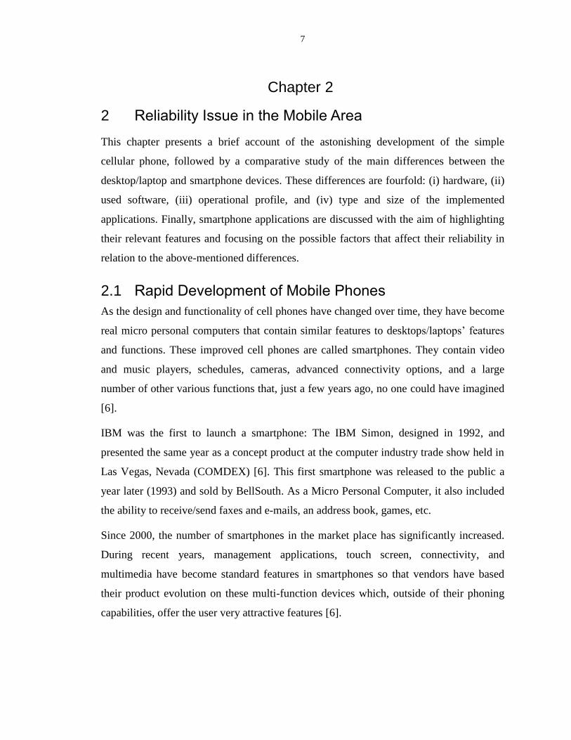
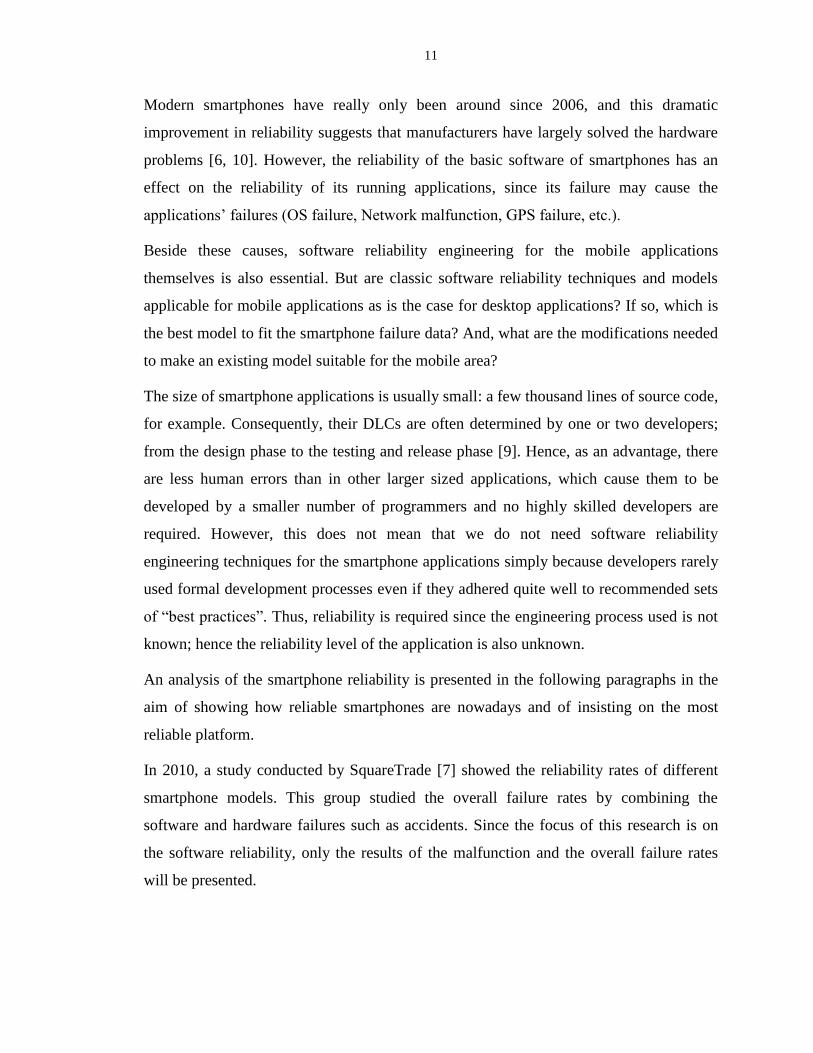
Figure 2-1 : Malfunction rates for various smartphone models [7]

The chart above reported the malfunction rate of the different smartphone models after 12

months. Based on those statistics, iPhone appears to be the most reliable, followed by

Android. In the first 12 months, fewer than 2.5% of the users that own an iPhone or

Motorola reported a malfunction. Followed by 3.7% of HTC users, and 6.3% of

Blackberry users, which is the highest rate recorded among the examined models. The

other smartphones examined together reported the worst rate which is 6.7%. Comparing

13

to the same study in 2008 by SquareTrade, smartphone reliability is improving, even for

Blackberry. In 2008, Blackberry had a malfunction rate of 9.1%, compared to 6.7% in

2010, and 3.4% for the iPhone, compared to 2.2%. This is a good example of the

improvements of smartphones, from the less reliable (Blackberry) to the most reliable

(iPhone) [7].

Those numbers also show that the malfunction rates of smartphones have dropped by

60%. This means that manufacturers, despite the fact that modern smart devices have

only really started gaining traction in 2006, have continued to solve their devices’

problems and have achieved remarkable improvement in reliability.

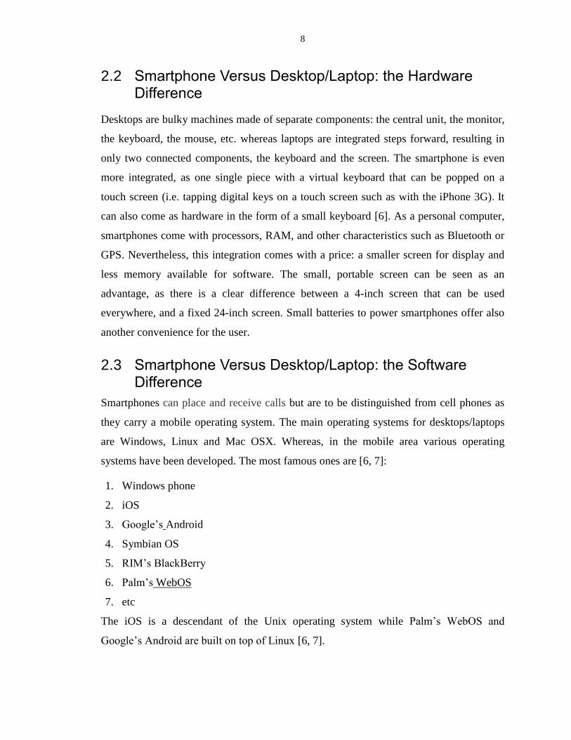
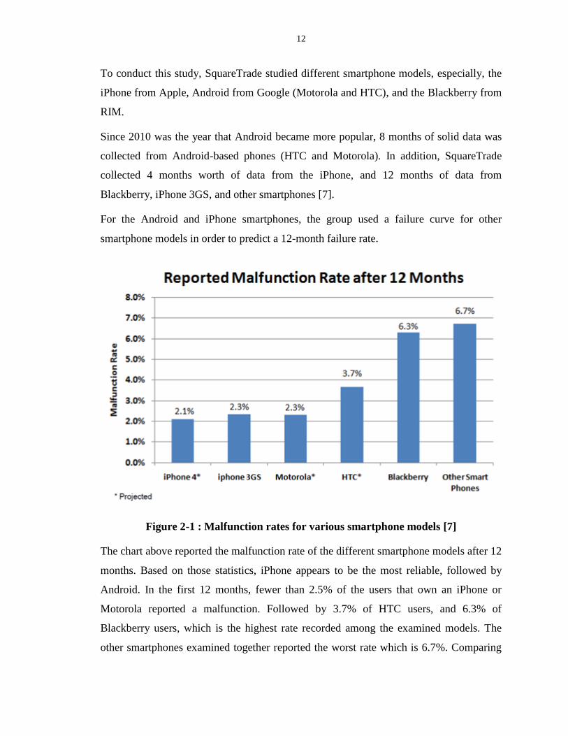
The following chart confirms that smartphone devices are the second most reliable

portable electronic devices, after digital cameras, with a malfunction rate of 3.9% over a

12-month usage, comparing to other devices.

Figure 2-2 : Reliability of portable electronic devices [7]

The DLC of a smartphone application is too short compared to that of a standard

application. Thus, developers do not usually track and collect enough metrics from their

applications [9]. Hence, increasing reliability is needed since we now have access to

14

critical applications such as online banking, stock exchange, etc. that might cause a first

level severity failure if they are not reliable enough.

In addition to the reliability of its applications, the smartphone reliability depends heavily

on the reliability of its operating system that should be studied as well since it could be

the reason for an application’s failure by rejecting its version, or any other reason.

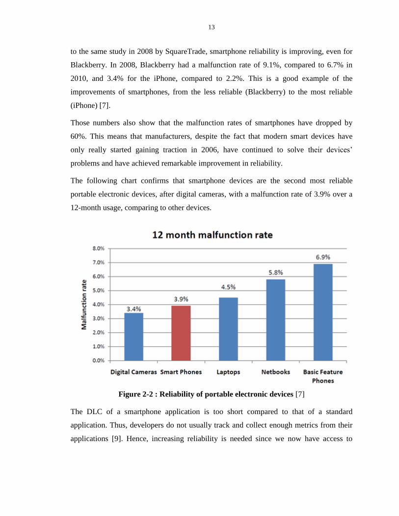
2.5.3 Smartphone Operating System Reliability

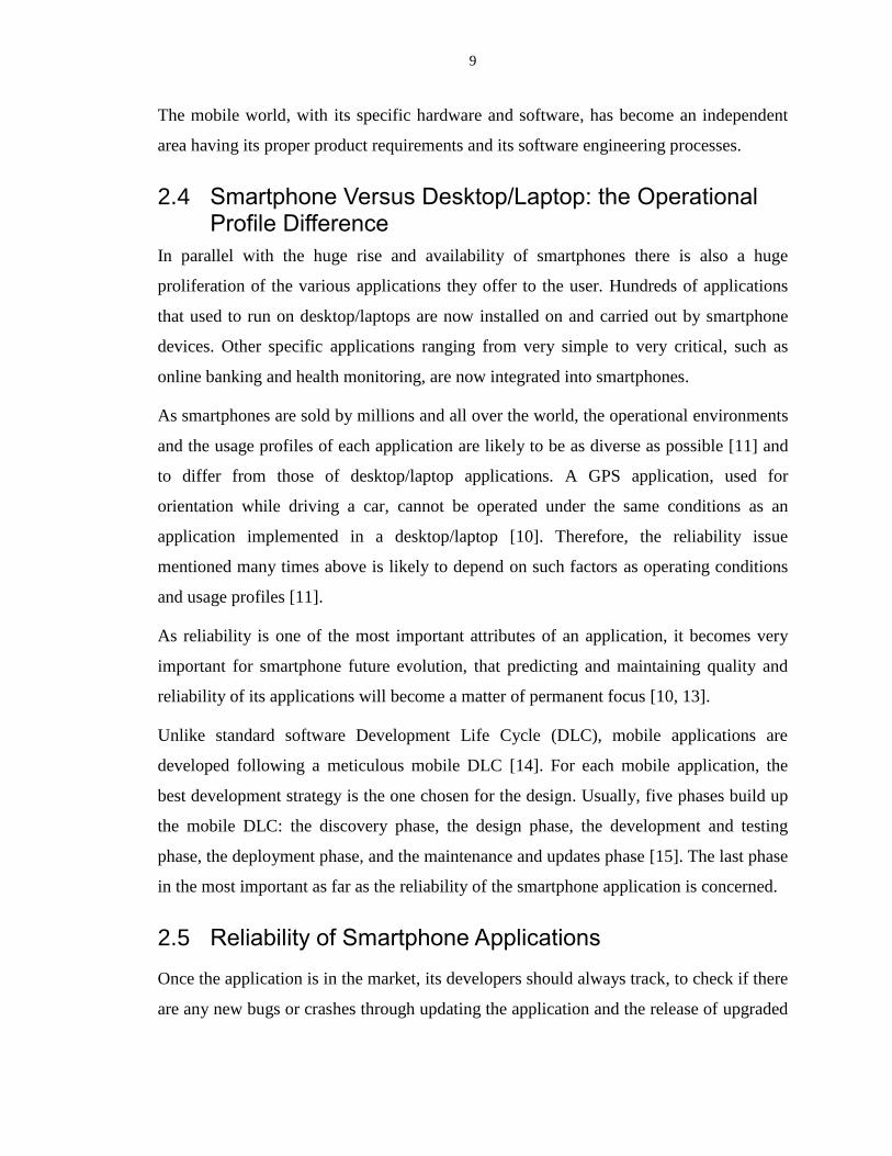
Nielsen Company [18] reported in October 2010 that Android was the most popular OS

among smartphone owners. A six-month study conducted by this company showed that

Android is quickly gaining traction (from 14% to 32%), while Apple iOS and Blackberry

RIM are in a significant decline (from 34% to 26% for the RIM OS and from 32% to

25% for the Apple iOS), as is illustrated in the following chart.

Figure 2-3 : Compared mobile operating systems reliability [19]

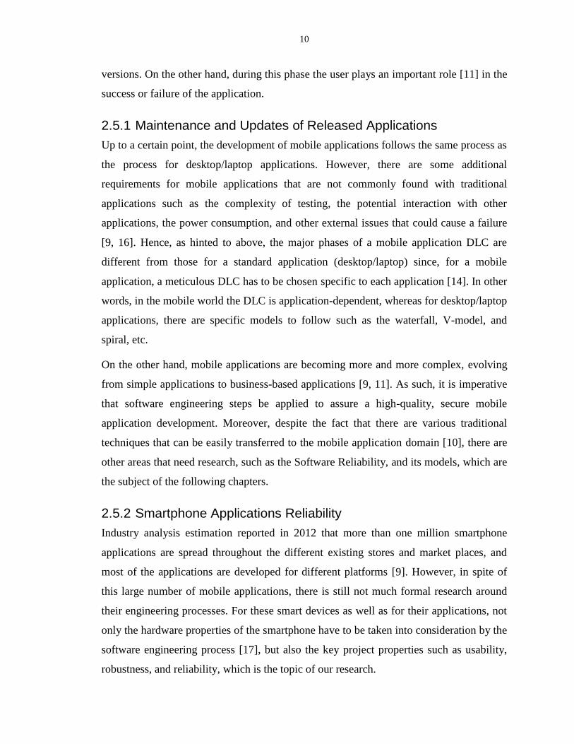
For the same period, Nielsen Company reported the top three OS share. The results are

presented in Figure 2-4. The chart shows the growth of the Android OS’ share and the

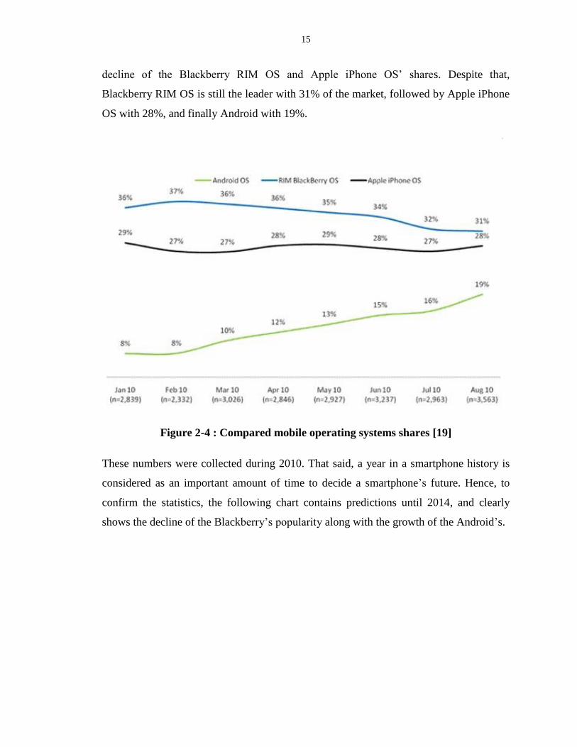
15

decline of the Blackberry RIM OS and Apple iPhone OS’ shares. Despite that,

Blackberry RIM OS is still the leader with 31% of the market, followed by Apple iPhone

OS with 28%, and finally Android with 19%.

Figure 2-4 : Compared mobile operating systems shares [19]

These numbers were collected during 2010. That said, a year in a smartphone history is

considered as an important amount of time to decide a smartphone’s future. Hence, to

confirm the statistics, the following chart contains predictions until 2014, and clearly

shows the decline of the Blackberry’s popularity along with the growth of the Android’s.

16

Figure 2-5 : Expected Smartphone user share, by OS [20]

This growth in usage shows the degree of reliability of smartphone OS. Yet this

reliability is based more on the hardware and lately, even more, on the OS than on the

application itself. Despite this, smartphone owners do not use the OS itself but the

application. Thus, the reliability of the application has to be studied independently from

the OS’ reliability, to assure a high-quality and better performance, especially for the

business-based applications. Although there are various traditional software engineering

techniques that can be easily transferred to the mobile area, there are still some research

issues in the mobile software reliability domain, namely:

How does one ensure the reliability of a smartphone application?

Can we apply directly the software reliability models that exist for desktop/laptop

applications to smartphone applications to estimate and predict their reliability?

Are the failure data enough to predict smartphone applications reliability, or do

we need to consider the external causes of the application’s failure (such as OS

versions, network failure, memory, CPU performance, power consumption, etc.)?

17

Is there a standard unique reliability model that can be applied to predict the

reliability of all smartphone applications? Or, is there a need for a meticulous

model for each type of application as is the case for their development models?

In the case of choosing among many available reliability models, is there a simple

criterion on which to base our choice?

2.6 Summary

Despite the large number of current mobile applications this seems to confirm that their

development processes are clear and understood, yet there are still an important number

of research issues that need to be studied. This chapter highlighted the differences in

hardware between desktops/laptops and smartphones as well as the differences in used

software, in particular, the reliability and the performances of the existing smartphone

operating systems, and stressed the incidence of the DLC of an application on its

reliability.

A reliability model, needed for smartphone applications is suggested. In the following

chapter, the mathematical reliability modeling and the three software reliability models

used later in our experimentation are presented.

18

Chapter 3

3 Software Reliability Growth Models: A Road Map

After briefly reviewing the major reliability concepts, three Software Reliability Growth

Models (SRGMs) used later in our experiments are presented: the Non-Homogenous

Poisson Process (NHPP) - Crow-AMSAA model (also termed the NHPP-Power Law

model), the Musa-Basic execution time model (or the exponential model), and the Musa-

Okumoto model (or the Logarithmic Poisson model). Analytic expressions for the

optimum values of the parameters of these models are derived using the Maximum

Likelihood Estimate (MLE) method and two common goodness-of-fit tests, namely the

Cramer-von Mises and the Chi-Squared are presented.

3.1 Mathematical Software Reliability Modeling

Software is omnipresent in our daily life. It is implemented in home equipment, in

telecommunications, in automobiles, in airplanes, etc. It is rapidly increasing in size and

complexity, and its proper functioning or its reliability is becoming a major concern. This

is reflected in the emerging and rapidly growing field of Software Reliability Engineering

(SRE) [21]. One of the techniques of SRE is the mathematical modeling of software

reliability. The purpose behind developing reliability models is the measurement,

estimation, and prediction of software reliability, the most important quality of software.

It is also a quantitative measure of software failures. A software reliability model

describes the behavior of the random process underlying software failures with respect to

time. A failure is a departure of the software output from its requirements. The basic

principle of each model is to accurately fit the observed failure data with a pre-specified

formula with some free parameters that have to be estimated by statistical methods such

as the least square or the maximum likelihood estimate techniques. The model can then

be used to estimate the current reliability or make predictions about future reliability of

the software and compare it to an objective reliability required by the costumer [21].

19

3.2 Reliability Concepts

The most used definition of software reliability is: “Software Reliability is the probability

of failure-free software operation for a specified period of time in a specified

environment” [21]. The mathematical modeling of software reliability, often called

reliability theory, is mainly the application of probability theory concepts to the modeling

of the failure data of hardware or software system. The concepts for repairable and non-

repairable systems are slightly different. Therefore, in the following, the two concepts are

examined separately.

3.2.1 Non-Repairable Systems

Non-repairable systems are defined as systems that become useless and discarded after

their first failure. The best example of a non-repairable system is a light bulb. It could

also be an electronic component inside a computer. Their lifetime is described by a

random variable, denoted , which is their time to failure. Starting from , we begin

by defining the probability that the time to failure of a non-repairable system, is

between and : Probability that . is a random

variable that can have values from to infinity. This probability can be written as:

(3.1)

where f(t) and F(t) are the probability density function and the cumulative distribution

function, respectively. Taking the limit of an infinitesimal time interval, the second

equation leads to:

(3.2)

which, following integration gives:

∫

(3.3)

using F(0) = 0. Thus F(t) is nothing but the probability of failure by time t:

∫

(3.4)

20

At this point, a more precise and quantitative definition of the reliability function,

denoted , can be given: it is just the probability of survival (or success) or failure-free

operation until time :

∫

(3.5)

where the normalization of the probability density function f(x) is used. Another useful

concept in reliability theory is the failure rate. It is defined as the probability that a failure

per unit time occurs in the time interval , , provided that the system had survived

without failure until time t; it is a conditional probability:

|

(3.6)

and the closely related concept of hazard rate by taking the limit of infinitesimal time

interval:

(3.7)

which is the instantaneous failure rate at time t. The hazard rate , usually

undistinguished from the failure rate, is a key variable in reliability theory as it allows

access to all the other variables. It has also the following appealing significance:

Probability that a system of age t will fail in the time interval , .

The average value of the time to failure is called the Mean Time to Failure (MTTF) and

is given by:

MTTF =∫

∫

(3.8)

The last equation follows from integration by parts. From the above definitions, one can

show easily the following relationships [21]:

21

0

R t exp[ z x dx] 1 F t

t

(3.9)

(3.10)

The general time dependence of the hazard rate, born from experience, is the so-called

“bathtub curve” with its three phases in the lifetime of the system [21].

3.2.2 Repairable Systems

A repairable system is a system which, upon failure, is restored to operation by a repair

action. These systems can be described by the following random variables [22]:

The total number of failures by time t. This cumulative number of failures is

always increasing with time. It gives the failure history of the system.

The time intervals between successive failures .

The number of failures , , in each time interval ] , where

and are the end times of the and the time interval.

These data types are not independent and can be transformed from one to the other. If we

consider a large number of identical systems (all identical smartphones in London, for

example) and record the failure history of each one starting from , we can

define the mean cumulative function by averaging over all the histories at each instant of

time. This function will give an average behavior. It is the mean value of that will

be denoted by:

(3.11)

The derivative of this mean value function is called the Rate Of oCcurrence Of Failures

(ROCOF), or Recurrence Rate (RR), and also called the failure intensity, denoted by

(3.12)

22

The failure intensity can be quite different from the hazard rate which was defined for

non-repairable systems [22]. The dimension of the failure intensity is (Number of failures

/ Unit of time).

Another useful concept for repairable systems is the Mean Time Between Failure

(MTBF), defined as the inverse of the failure intensity. An increasing MTBF is indicative

of a reliability growth, whereas a decreasing MTBF is indicative of reliability

deterioration.

The purpose of all reliability models, designed for repairable systems, such as

smartphones, is to arrive at a suitable expression for the mean value cumulative function

based on appropriate assumptions. In the following section, the three most used reliability

models are presented.

3.3 Three Most Used Software Reliability Growth Models

The first Software Reliability Growth Model (SRGM) was developed in 1972 [21, 23].

SRGMs were initially designed to assess the evolution of software in its successive

testing phases. As a result of the corrective actions taken during these phases, the

software reliability increases, expressed by the word “growth” (compared to software

with a constant failure rate, where no repair actions are planned). These models have also

been found to describe adequately the reliability of fielded complex systems, i.e. in the

user environment [24]. Relying on simplifying assumptions [21], a SRGM usually results

in a set of mathematical equations that accurately fit the collected failure data.

There are some basic assumptions that are shared by all of the models. These common

assumptions, referred to as the standard assumptions, are [21]:

The software is operated in a similar manner as that in which reliability

predictions are to be made, i.e., during the testing phase, the software is executed

in a manner similar to the anticipated operational usage.

Every fault has the same chance of being encountered within a severity class as

any other fault in that class.

23

The failures, when the faults are detected, are independent. This assumption

allows a simple estimation of the model parameters by using the joint density

probability functions.

There are additional assumptions, specific to each particular model. However, some of

these assumptions may not comply with real situations [25]. The assessment and validity

of the most used assumptions, and their conformity to real observations, will be examined

in the next chapter. In the following sections, the three Software Reliability Growth

Models (SRGM) mentioned above are presented.

3.3.1 The NHPP Crow-AMSAA Model

The first Non-Homogenous Poisson Process (NHPP) model was presented by Amrit Goel

and Kazu Okumoto in 1979 [21]. In this model, the failure event is modeled by an NHPP

distribution where it is assumed that there exists a mean value function giving the

expected number of failures up to a given time. It was successfully used as a Hardware

Reliability Growth Model. Because of its simplicity and easy implementation, there are

several models that have since been developed, based on the NHPP model. In addition to

the above Standard Assumptions, there are some others specific to each variant of the

NHPP model, that help determine the mean value and other useful equations of the

model, in order to predict the software reliability. Those assumptions are detailed in [21].

Including the Standard Assumptions mentioned above, in a NHPP model, the added

assumption is that the probability distribution obeyed by the random variable

follows a Poisson Process i.e. is given by:

]

(3.13)

where is the mean value of or the expected cumulative failure number:

(3.14)

The failure intensity is:

(3.15)

24

In a NHPP model, the reliability of a system at time , defined as the probability of failure

free operation until time :

] ( ) (3.16)

Therefore, the cumulative probability distribution which is the probability of failure by

time is:

(3.17)

and the probability density function is given by:

(3.18)

On the other hand, if we denote by , , the number of failures in the time

interval ] , where and are the end times of the and the

time interval, then, in a NHPP model:

n

i 1   i  

i   i 1   i  

µ T µ TPr f n exp( µ T µ T

n!

(3.19)

which means that the number of failures in each time interval follows a Poisson

distribution with mean value ( ). The particular NHPP model used in

this work and implemented in the Reliability Growth Analysis (RGA) tool is called the

Crow-AMSAA model [24], or the NHPP-Power Law model. This model was first

developed by the U.S. Army Material Systems Analysis Activity (AMSAA). It was an

extension of an earlier model called the Duane model [21]. The main idea is that the

failure intensity is linear when plotted on a log-log scale, as a function of time.

In the NHPP Crow-AMSAA model, the expected value of is written as:

, λ > 0 ; β > 0 (3.20)

It is a two parameter model, λ and β. Therefore, the probability distribution reads:

]

(3.21)

and the instantaneous failure intensity is given by:

25

λ(t) (3.22)

or on a log-log scale:

( ) (3.23)

( ) (3.24)

These can be represented by straight lines of slope and respectively.

The instantaneous Mean Time Between Failures (MTBF) is defined as:

MTBF(t) =

λ (3.25)

Beside the instantaneous failure intensity and the instantaneous Mean Time Between

Failures (MTBF), one can define the cumulative failure intensity and the cumulative

Mean Time Between Failures by the following relations:

(3.26)

and

(3.27)

Plotted on a log-log scale, the lines representing the instantaneous and cumulative failure

intensity have the same slope and are therefore parallel; the same is true for the

instantaneous and cumulative MTBFs.

The reliability of a repairable system following the NHPP Crow-AMSAA model is

therefore:

(3.28)

and the probability density function (pdf) is given by:

(3.29)

Three cases are worth noting:

26

β=1 is called the Homogeneous Poisson Process (HPP). This case corresponds to

a constant failure intensity (λ(t) and a constant MTBF (

( )

). The

reliability in this case is given by:

(3.30)

β < 1 in this case the failure intensity is decreasing and the MTBF is increasing.

The reliability in this case is given by:

(3.31)

denoting a reliability growth.

β > 1 in this case the failure intensity is increasing and the MTBF is decreasing.

The reliability in this case is given by:

(3.32)

indicating a decrease in reliability and a resulting deterioration.

Finally, to implement this model, either the fault counts or the time between failures are

required.

3.3.2 Musa’s Basic Execution Time Model

The simple and intuitive idea behind this model is that as the cumulative number of

failures increases and the corresponding faults are fixed; as such, the failure intensity

should decrease. Including the Standard Assumptions, the additional assumptions of this

model are:

The failure intensity decreases is modeled by the simple linear equation [26]:

(3.33)

where:

- µ is the mean (or expected) cumulative number of failures observed at execution

time τ.

- is the initial failure intensity (at the beginning of the observations) at τ = 0.

27

- is the total number of expected system failure if the observation lasts for an

infinite time.

Writing the failure intensity as the derivative of the cumulative number of failures, this

leads to the following differential equation satisfied by the function (τ):

τ

(3.34)

whose solution, for the mean value of failure counts, and for the failure intensity as

functions of execution time, are given by:

µ(τ) = (

τ)] (3.35)

(

τ) (3.36)

and constitute The Musa-Basic model, also termed the exponential model [28]. If the

present failure intensity is and the target failure intensity is required, then the

expected number of failures and the additional execution time required to reach that

objective are given by:

Δ =

(3.37)

Δτ =

) (3.38)

This model is used especially for execution time data but it can also be applied to

calendar time data by applying a conversion from calendar to execution time. The

required data to build this model are either the time of failure or time between failures.

Based on the software reliability modeling survey from the handbook of SRE [21], this

model is considered to be one of the most widely used models [21, 28].

There are several similar models that have been developed. Moreover, Musa mentioned

that “the basic execution model generally appears to be superior in capability and

applicability to other published models” [28, 29].

28

3.3.3 Musa-Okumoto Logarithmic Poisson Model

According to Farr [21, 28], the Musa-Okumoto model, also termed the Logarithmic

Poisson model, is one of the most extensively applied models. Besides that, Musa himself

confirmed that this model is more accurate comparing to the exponential model [29].

Including the Standard Assumptions, the additional assumption of this model is that,

contrary to the exponential model, the failure intensity decrease is not linear but more

rapid and modeled by an exponential equation:

(3.39)

where:

- is a measure of the decrease in failure intensity in the logarithmic model

- is the initial failure intensity (at the beginning of the observations) i.e at τ = 0.

As for the previous model, the mean value is the solution of the following differential

equation:

τ (3.40)

whose solution gives the mean cumulative failure number and the failure intensity as

functions of the execution time [28] :

µ(τ) =

(3.41)

τ

τ (3.42)

The required data to build this model are the same as for the exponential model. As one

of the best predictive models, the Musa-Okumoto model belongs to the selected models

in the AIAA Recommended Practice Standard on Software Reliability [21]. Logarithmic

models have been also used in software cost estimation models with high accuracy [27,

30, 31].

Further details on the Musa-Basic and Musa-Okumoto models can be found in [21].

29

3.4 Parameters Estimation

Once a reliability growth model is chosen, four basic steps have to be followed:

Estimate (optimize) the parameters of the model using statistical techniques such

as the Maximum Likelihood Estimate (MLE), or the Least Square Estimation

(LSE) method,

Substitute the optimum values of the parameters obtained in the previous step,

into the selected model.

Perform a goodness-of-fit test to assess the reasonableness of the model. If the test

is conclusive, the data are adequately described by the chosen model, otherwise

the model is rejected and another one is chosen.

Draw conclusions about the reliability of the system based on the fitted model.

Schematic representations of these steps are summarized in the following figure:

Figure 3-1: Use of a chosen SRGM to study the reliability of an application [32, 33]

The choice of the selected model is based on an examination of the general trend of the

observed cumulative failure number curve as a function of time. For the estimation

30

of the parameters of a given model, two widely known methods are used: the Maximum

Likelihood Estimate (MLE), and the Least Square Estimation (LSE) method. As the LSE

is a standard technique in numerical analysis; in the following, only the MLE method is

presented.

3.4.1 The Maximum Likelihood Estimate (MLE)

The MLE is the most important and widely used estimation technique. It is based on the

idea that the failure data observed (the successive failure events of the studied system) are

the most likely to happen i.e. are the most probable ones (have the maximum

probability).

3.4.2 The Case of Failure Times Data Type

If we denote by . the observed failure times arranged in an increasing

order. For the NHPP model, the probability density function (pdf) of the failure

occurring at time , given that the failure has occurred at is given by the

conditional probability [21]:

|

( )

( ) (3.43)

Based on the third assumption of the above mentioned Standard Assumptions

(independence of occurring failures), the likelihood or the probability of having the

observed successive failure times is:

∏ |

(3.44)

In the case of the Crow-AMSAA model, it is written as [24]:

∏

(3.45)

The optimal parameters of the model are those values of λ and β that give the maximum

likelihood i.e. the maximum value of or of its logarithm:

Λ

∑ (3.46)

31

Therefore, to get the optimum values of parameters λ and β, the following system of

equations should be solved:

{

∑

(3.47)

whose solution λ are:

∑

(3.48)

(3.49)

For the case of Musa’s basic execution time model and the Logarithmic Poisson model, a

similar analysis leads to the optimal model parameters values, given in [21].

3.4.3 The Case of Grouped Data Type

In this case, the data are grouped by time intervals, giving the number of failures in each

interval. If we denote by the observed number of failures in the time interval, then

the likelihood function for the Crow-AMSAA model, is given by:

∏

∏

(3.50)

where is the total number of intervals and is the end of the time interval. Using

the same procedure as in the previous data type case, the optimum values of the

parameters are obtained. The parameter β is a solution of the following equation:

∑ [

]

(3.51)

whereas λ (in equation 3.50) is given by:

(3.52)

32

where is the solution of the previous equation (equation 3.51). and are the values

of λ and β that maximize the likelihood function L.

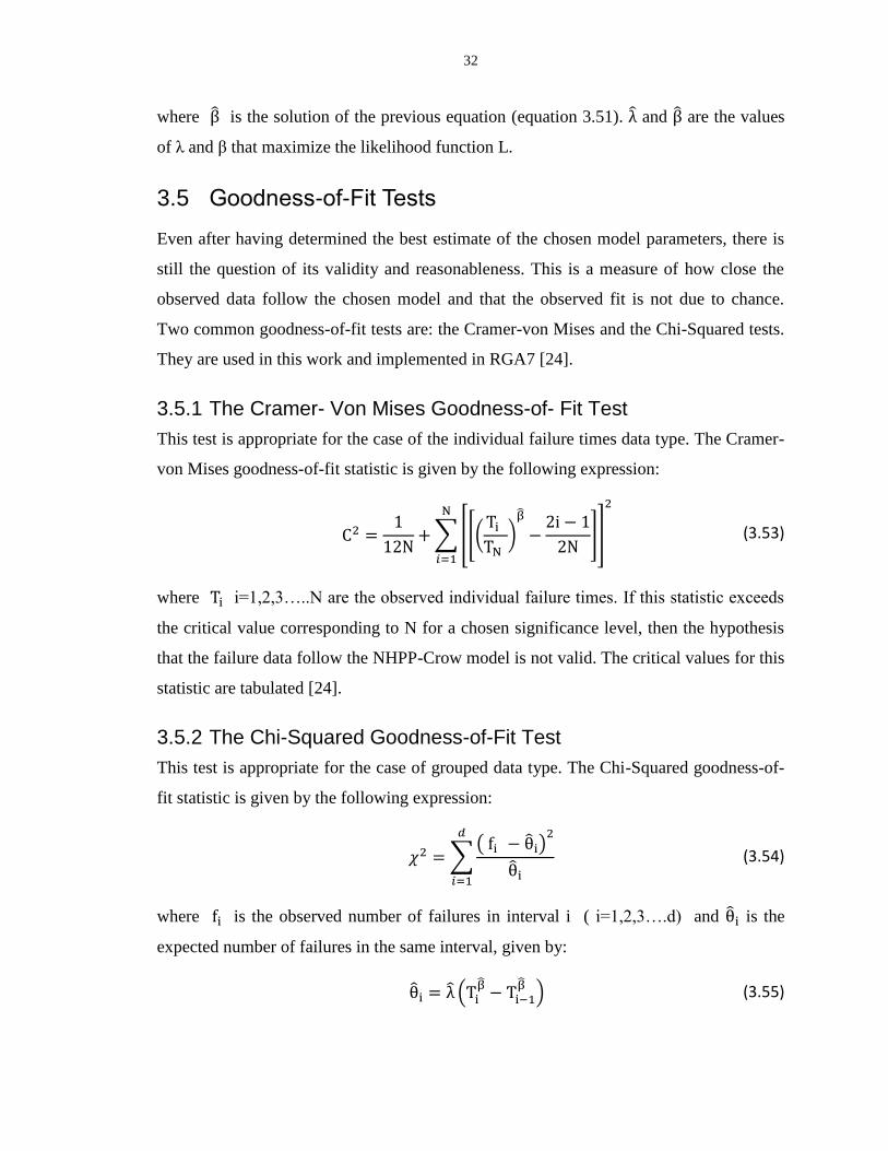
3.5 Goodness-of-Fit Tests

Even after having determined the best estimate of the chosen model parameters, there is

still the question of its validity and reasonableness. This is a measure of how close the

observed data follow the chosen model and that the observed fit is not due to chance.

Two common goodness-of-fit tests are: the Cramer-von Mises and the Chi-Squared tests.

They are used in this work and implemented in RGA7 [24].

3.5.1 The Cramer- Von Mises Goodness-of- Fit Test

This test is appropriate for the case of the individual failure times data type. The Cramer-

von Mises goodness-of-fit statistic is given by the following expression:

∑[[(

)

]]

(3.53)

where i=1,2,3…..N are the observed individual failure times. If this statistic exceeds

the critical value corresponding to N for a chosen significance level, then the hypothesis

that the failure data follow the NHPP-Crow model is not valid. The critical values for this

statistic are tabulated [24].

3.5.2 The Chi-Squared Goodness-of-Fit Test

This test is appropriate for the case of grouped data type. The Chi-Squared goodness-of-

fit statistic is given by the following expression:

∑

( )

(3.54)

where is the observed number of failures in interval i ( i=1,2,3….d) and is the

expected number of failures in the same interval, given by:

(

) (3.55)

33

If this statistic exceeds the critical value corresponding to ((d-2), where d is the number

of intervals) for a chosen significance level, then the hypothesis that the grouped failure

data follow the NHPP-Crow model is not valid. The critical values for this statistic can be

found in tables of the Chi-Squared distribution.

3.6 Summary

In this chapter, the main reliability concepts are recalled, and three most used SRGM

models are presented, as well as the estimation of their parameters, followed by the two

common goodness-of-fit tests. In the next chapter, these models will be applied to the

collected failure data of three smartphone applications in order to assess the reliability of

their software and consequently, test whether the chosen models perform equally well in

the mobile area as in that of desktop/laptop.

34

Chapter 4

4 Smartphone Failure Data and Application of SRGMs

As previously emphasized, reliability is one of the most important features of an

application and great efforts have been devoted to tailor and predict it through the study

of recorded failure data. A non-reliable application leads to dissatisfied customers, loss of

market share, and significant costs to the supplier. For critical applications, such as

banking or health monitoring, non-reliability can lead to great damage. Therefore, it is of

great necessity to ensure early detection and resolution of reliability issues in desktop

applications as well as, now increasingly, in mobile applications.

This chapter is devoted to a detailed presentation of the main purpose of this work [41,

42], namely the application of three Software Reliability Growth Models, known to be

successful in the desktop/laptop area, to three concrete cases of smartphone applications.

The Software Reliability Growth Models used later in our experiments are: the NHPP -

Crow-AMSAA model (also termed the NHPP-Power Law model), the Musa-Basic

execution time model (or the exponential model), and the Musa-Okumoto model (or the

Logarithmic Poisson model) and the chosen applications are: Skype, Vtok, and a private

Windows phone application.

The detailed procedure devised to collect the failure data for each application is presented

first, followed by the results of the application of the chosen SRGM to each application’s

failure data and, finally, a detailed analysis of the observed results. The collected failure

data for each application are reported in appendix A.

4.1 Data Collection

We used Apple devices (iPhone, iPad, iPod Touch) crash files as well as a Windows

phone crash file as our “experimental” data. These crash files are not public, therefore are

confidential. Hence, we will focus more on the Apple devices crash files since it was

easier to collect them from our personal devices as well as through a survey that was sent

to different people from different parts of the world. There are those who gratefully

accepted to send us their failure data, whereas other did not.

35

For the Windows phone case, we could only get the crash file report of one application

due to confidentiality policies. Collecting the data was, and still is, a challenge especially

for Android devices which is left as future work.

Figure 4-1 presents an example of the Apple devices crash log. For each case, we provide

the following information:

Name of the crashed application

Type

Hardware type (device as iPhone, iPad or iPod Touch). This information is

needed in order to determine whether the crash is of an application of the same

device or of the same application from a different device

Date/Time of the crash (which is the most important information in the crash log

for our research work)

The version of the OS

The crash logs of Apple devices are transferred to a hidden folder located/created in the

PC that is used for the synchronization of the device. It contains the crash logs of all of

the applications installed on the devices, as well as reports about the battery, memory,

and other features. However, we are only interested in the crash files. Thus, we ignored

the other files.

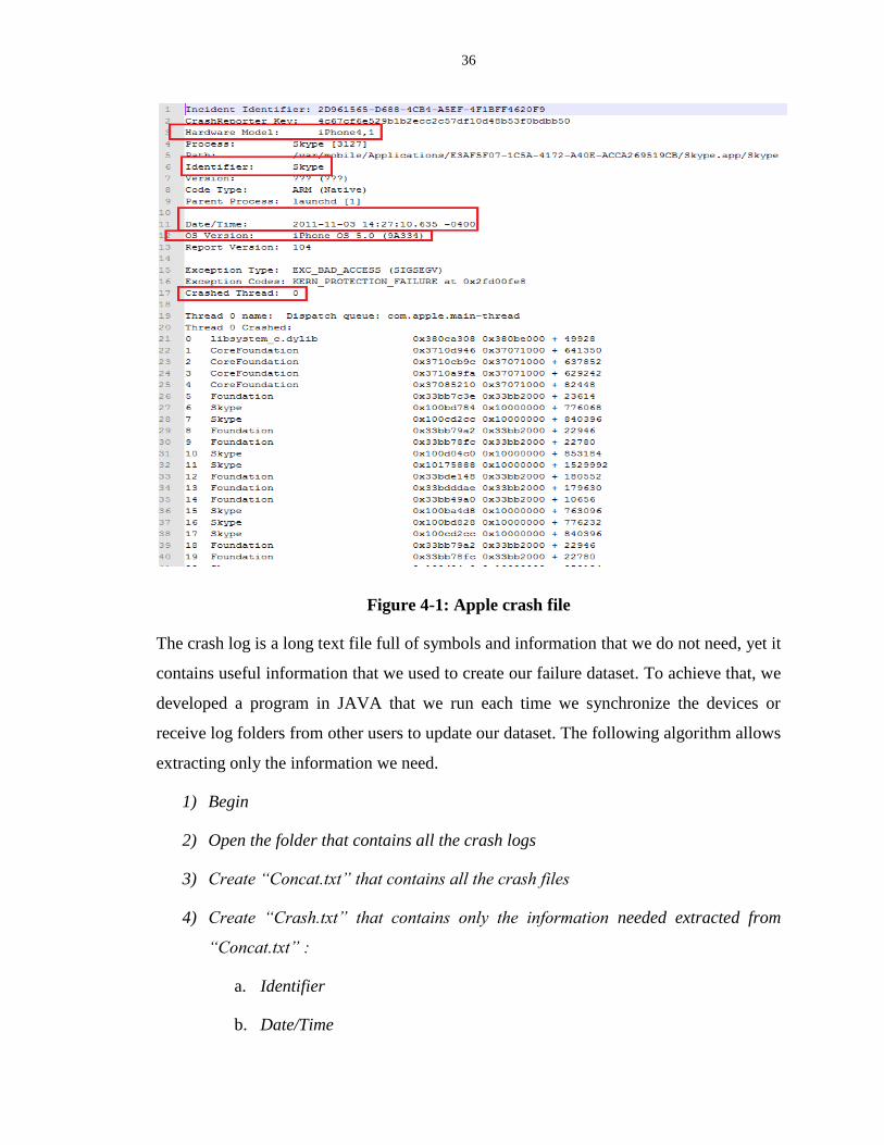
36

Figure 4-1: Apple crash file

The crash log is a long text file full of symbols and information that we do not need, yet it

contains useful information that we used to create our failure dataset. To achieve that, we

developed a program in JAVA that we run each time we synchronize the devices or

receive log folders from other users to update our dataset. The following algorithm allows

extracting only the information we need.

1) Begin

2) Open the folder that contains all the crash logs

3) Create “Concat.txt” that contains all the crash files

4) Create “Crash.txt” that contains only the information needed extracted from

“Concat.txt” :

a. Identifier

b. Date/Time

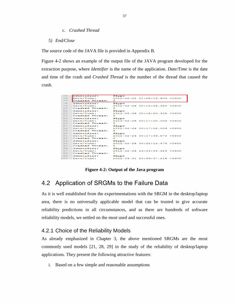
37

c. Crashed Thread

5) End/Close

The source code of the JAVA file is provided in Appendix B.

Figure 4-2 shows an example of the output file of the JAVA program developed for the

extraction purpose, where Identifier is the name of the application. Date/Time is the date

and time of the crash and Crashed Thread is the number of the thread that caused the

crash.

Figure 4-2: Output of the Java program

4.2 Application of SRGMs to the Failure Data

As it is well established from the experimentations with the SRGM in the desktop/laptop

area, there is no universally applicable model that can be trusted to give accurate

reliability predictions in all circumstances, and as there are hundreds of software

reliability models, we settled on the most used and successful ones.

4.2.1 Choice of the Reliability Models

As already emphasized in Chapter 3, the above mentioned SRGMs are the most

commonly used models [21, 28, 29] in the study of the reliability of desktop/laptop

applications. They present the following attractive features:

i. Based on a few simple and reasonable assumptions

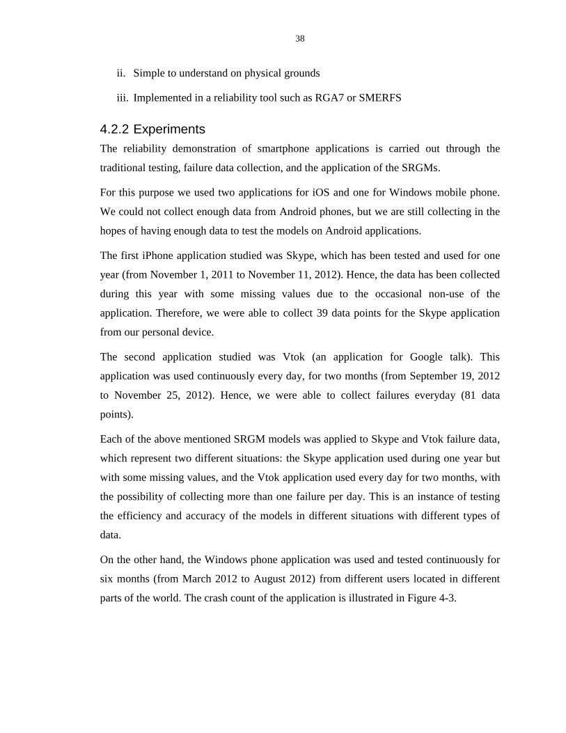
38

ii. Simple to understand on physical grounds

iii. Implemented in a reliability tool such as RGA7 or SMERFS

4.2.2 Experiments

The reliability demonstration of smartphone applications is carried out through the

traditional testing, failure data collection, and the application of the SRGMs.

For this purpose we used two applications for iOS and one for Windows mobile phone.

We could not collect enough data from Android phones, but we are still collecting in the

hopes of having enough data to test the models on Android applications.

The first iPhone application studied was Skype, which has been tested and used for one

year (from November 1, 2011 to November 11, 2012). Hence, the data has been collected

during this year with some missing values due to the occasional non-use of the

application. Therefore, we were able to collect 39 data points for the Skype application

from our personal device.

The second application studied was Vtok (an application for Google talk). This

application was used continuously every day, for two months (from September 19, 2012

to November 25, 2012). Hence, we were able to collect failures everyday (81 data

points).

Each of the above mentioned SRGM models was applied to Skype and Vtok failure data,

which represent two different situations: the Skype application used during one year but

with some missing values, and the Vtok application used every day for two months, with

the possibility of collecting more than one failure per day. This is an instance of testing

the efficiency and accuracy of the models in different situations with different types of

data.

On the other hand, the Windows phone application was used and tested continuously for

six months (from March 2012 to August 2012) from different users located in different

parts of the world. The crash count of the application is illustrated in Figure 4-3.

39

Figure 4-3: Windows phone crash count.

The failure rate is low in the spring period and very pronounced in the summer period,

due to intensive usage.

It is important to note that June, July, and August are the months with the highest crash

rates. Since this application is developed for the purpose of locating bicycle stations, it is

used during the summer period more than in the winter, which explains the high crash

rate during the hot season. This reflects the fact that the type of an application and its

usage play an important role in its reliability. From the graph we extracted the failure data

over the six month period.

We then used two software reliability tools to double check the results. The first tool is

the RGA7 from ReliaSoft [24], and the second one is Statistical Modeling and Estimation

of Reliability Functions for Software (SMERFS) [34]. We configured our tools as

follows: we chose 1 for the severity level of all failures and the time unit selected was

hour. As the time scales of the three applications are very different, we choose to

normalize our data between 0 and 1 using the following equation:

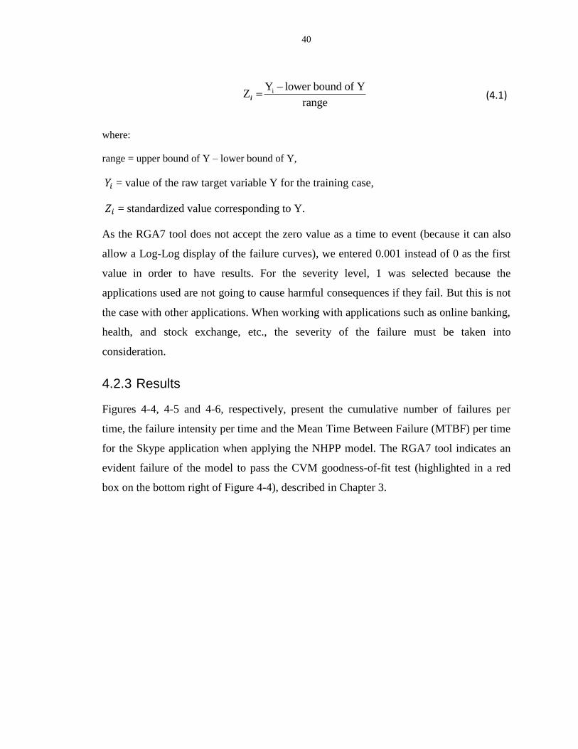
40

iY lower bound of YZ

range

i   (4.1)

where:

range = upper bound of Y – lower bound of Y,

= value of the raw target variable Y for the training case,

= standardized value corresponding to Y.

As the RGA7 tool does not accept the zero value as a time to event (because it can also

allow a Log-Log display of the failure curves), we entered 0.001 instead of 0 as the first

value in order to have results. For the severity level, 1 was selected because the

applications used are not going to cause harmful consequences if they fail. But this is not

the case with other applications. When working with applications such as online banking,

health, and stock exchange, etc., the severity of the failure must be taken into

consideration.

4.2.3 Results

Figures 4-4, 4-5 and 4-6, respectively, present the cumulative number of failures per

time, the failure intensity per time and the Mean Time Between Failure (MTBF) per time

for the Skype application when applying the NHPP model. The RGA7 tool indicates an

evident failure of the model to pass the CVM goodness-of-fit test (highlighted in a red

box on the bottom right of Figure 4-4), described in Chapter 3.

41

Figure 4-4: Cumulative number of failures and its mean value function per time for

the Skype application.

Note the failure occurrences in “bursts” followed by flat plateaus, a feature that cannot be

easily accommodated by the theoretical reliability model. The statistical Cramer-Von-

Mises test revealed that the chosen NHPP model failed to adequately reproduce the data.

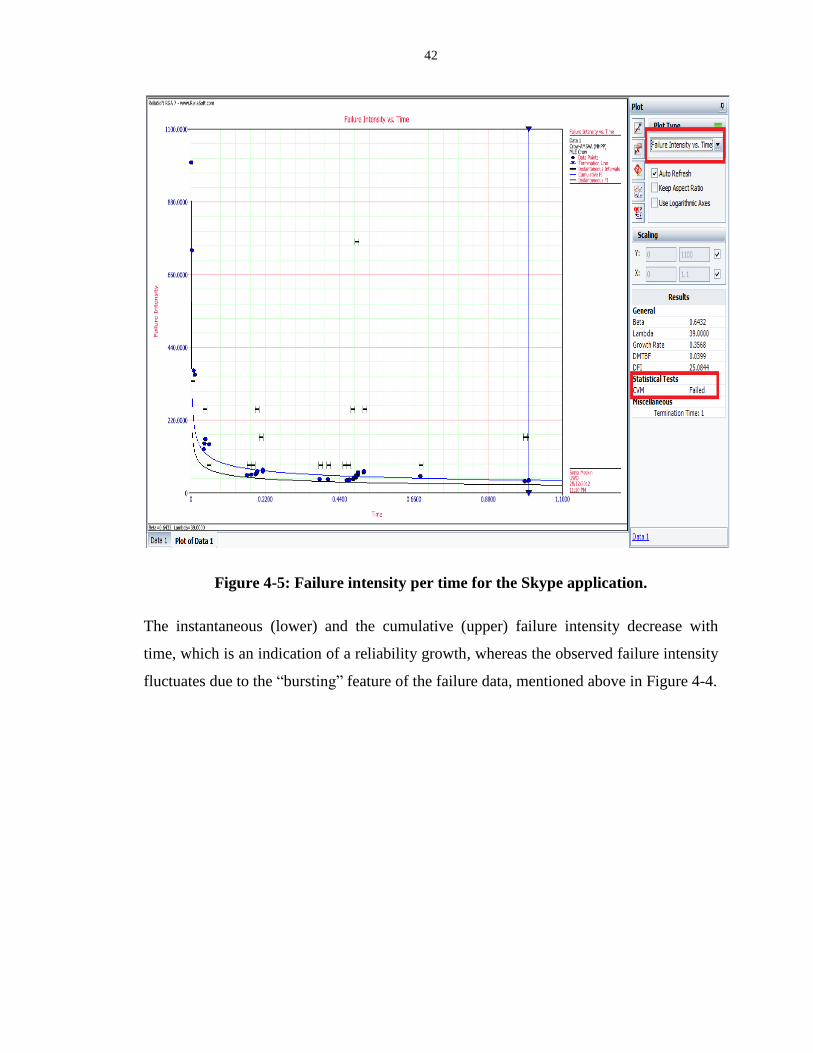
42

Figure 4-5: Failure intensity per time for the Skype application.

The instantaneous (lower) and the cumulative (upper) failure intensity decrease with

time, which is an indication of a reliability growth, whereas the observed failure intensity

fluctuates due to the “bursting” feature of the failure data, mentioned above in Figure 4-4.

43

Figure 4-6: Instantaneous (upper) and cumulative (lower) Mean Time Between

Failure MTBF of the Skype application.

The same previous comments apply. The MTBF is the reciprocal of the failure intensity

and is also a convenient measure of the reliability of an application. An overall increase

in the MTBF is indicative of a reliability growth, which is the case in these experiments.

Likewise, Figures 4-7, 4-8, and 4-9, respectively, represent the cumulative number of

failures per time, the failure intensity per time, and the MTBF per time of the Vtok

application. Again, the NHPP model failed to fit the data as indicated by the CVM

goodness-of-fit test (red rectangle at the bottom right of Figure 4-7 indicates the CVM

failure).

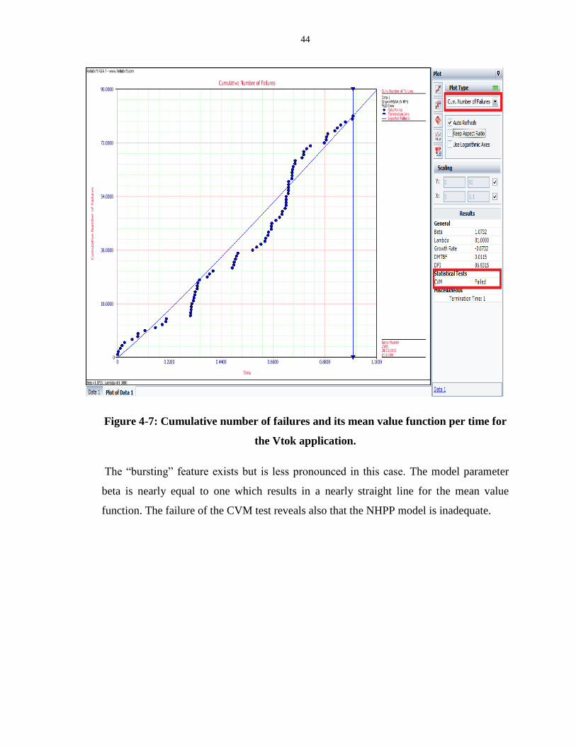
44

Figure 4-7: Cumulative number of failures and its mean value function per time for

the Vtok application.

The “bursting” feature exists but is less pronounced in this case. The model parameter

beta is nearly equal to one which results in a nearly straight line for the mean value

function. The failure of the CVM test reveals also that the NHPP model is inadequate.

45

Figure 4-8: Instantaneous (upper) and cumulative (lower) failure intensity per time

for the Vtok application.

The failure intensity is nearly constant during the observed period because the above

curve for the mean value function of the cumulative number of failures is nearly a

straight line (the failure intensity is the derivative of the mean value function).

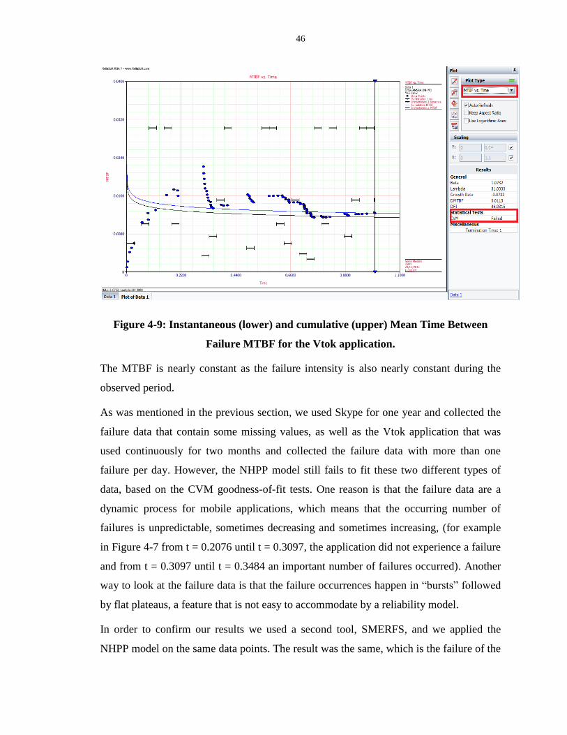
46

Figure 4-9: Instantaneous (lower) and cumulative (upper) Mean Time Between

Failure MTBF for the Vtok application.

The MTBF is nearly constant as the failure intensity is also nearly constant during the

observed period.

As was mentioned in the previous section, we used Skype for one year and collected the

failure data that contain some missing values, as well as the Vtok application that was

used continuously for two months and collected the failure data with more than one

failure per day. However, the NHPP model still fails to fit these two different types of

data, based on the CVM goodness-of-fit tests. One reason is that the failure data are a

dynamic process for mobile applications, which means that the occurring number of

failures is unpredictable, sometimes decreasing and sometimes increasing, (for example

in Figure 4-7 from t = 0.2076 until t = 0.3097, the application did not experience a failure

and from t = 0.3097 until t = 0.3484 an important number of failures occurred). Another

way to look at the failure data is that the failure occurrences happen in “bursts” followed

by flat plateaus, a feature that is not easy to accommodate by a reliability model.

In order to confirm our results we used a second tool, SMERFS, and we applied the

NHPP model on the same data points. The result was the same, which is the failure of the

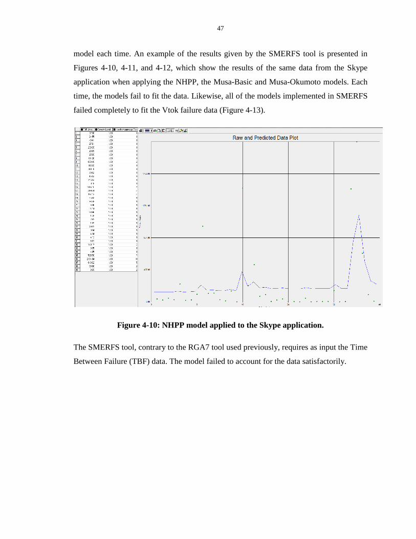
47

model each time. An example of the results given by the SMERFS tool is presented in

Figures 4-10, 4-11, and 4-12, which show the results of the same data from the Skype

application when applying the NHPP, the Musa-Basic and Musa-Okumoto models. Each

time, the models fail to fit the data. Likewise, all of the models implemented in SMERFS

failed completely to fit the Vtok failure data (Figure 4-13).

Figure 4-10: NHPP model applied to the Skype application.

The SMERFS tool, contrary to the RGA7 tool used previously, requires as input the Time

Between Failure (TBF) data. The model failed to account for the data satisfactorily.

48

Figure 4-11: Musa-Basic model applied to Skype failure data. Same as above.

Figure 4-12: Musa-Okumoto model applied to Skype failure data. Same as above.

None of the selected SRGMs fit the data.

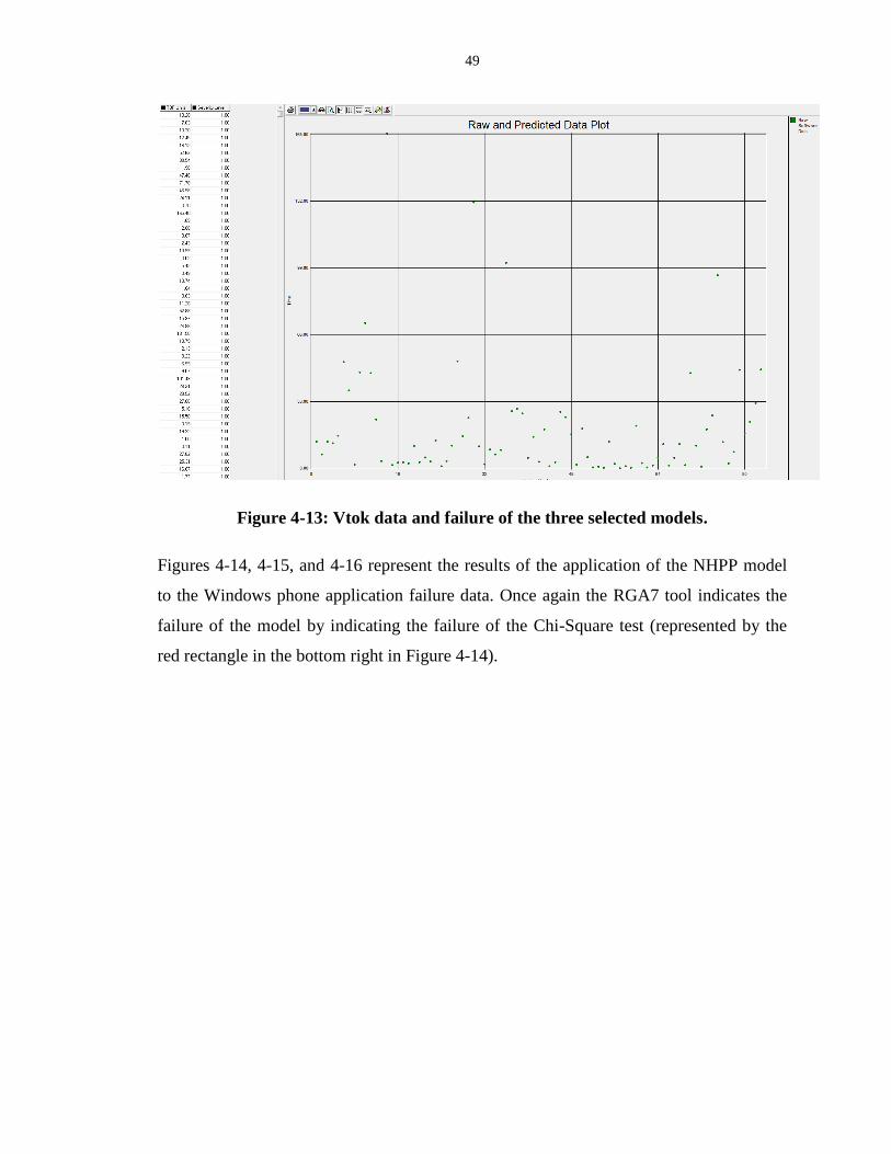
49

Figure 4-13: Vtok data and failure of the three selected models.

Figures 4-14, 4-15, and 4-16 represent the results of the application of the NHPP model

to the Windows phone application failure data. Once again the RGA7 tool indicates the

failure of the model by indicating the failure of the Chi-Square test (represented by the

red rectangle in the bottom right in Figure 4-14).

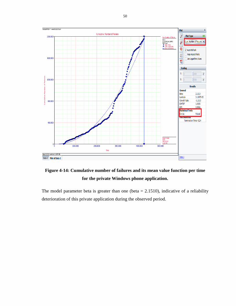
50

Figure 4-14: Cumulative number of failures and its mean value function per time

for the private Windows phone application.

The model parameter beta is greater than one (beta = 2.1510), indicative of a reliability

deterioration of this private application during the observed period.

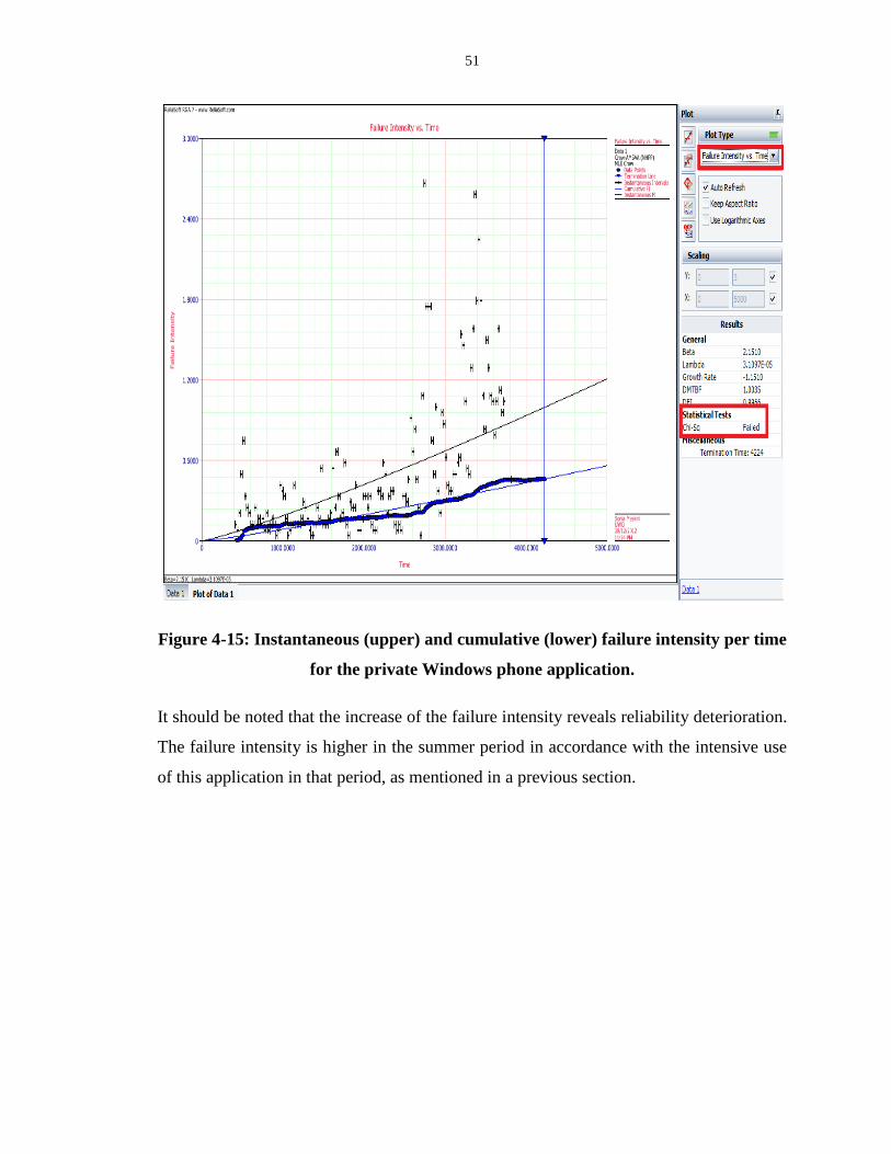
51

Figure 4-15: Instantaneous (upper) and cumulative (lower) failure intensity per time

for the private Windows phone application.

It should be noted that the increase of the failure intensity reveals reliability deterioration.

The failure intensity is higher in the summer period in accordance with the intensive use

of this application in that period, as mentioned in a previous section.

52

Figure 4-16: Instantaneous (lower) and cumulative (upper) Mean Time Between

Failure (MTBF) for the private Windows phone application.

Note the decrease of the MTBF, indicative of reliability deterioration for the observed

period.

4.3 Evaluation

Thus, the most successful reliability models [21, 28, 29] failed to fit all of the data and

failed to predict the reliability in the mobile area for smartphone applications. This failure

can be traced back to the following differences between desktops/laptops and

smartphones.

4.3.1 Operational Environments and Usage Profiles of Smartphone Applications

One of the mobile application failure characteristics is that they are application dependent

in the sense that they are dynamic and non-homogenously spread over time [16, 35].

Moreover, they are unpredictable, sometimes decreasing and sometimes increasing, i.e.

53

happening in “bursts”. One possible explanation is that reliability depends on the type of

the used application (for example, the Windows phone application mentioned earlier),

and on its operational environment and usage profile (where and when and how the

application is used). Because the usage may differ from one user to another, from one

country to another, from one condition to another [11], this explains the uncertainty of

usage of the application in the execution and release time [12], and all of these factors

play an important role in the reliability of the applications.

Another reason is that the DLC of a mobile application is short (up to 90 days) and the

programmer aims to develop the application as fast as possible to satisfy the time-to-

market constraint, which leads to skip phases from the DLC. The most skipped phase is

the design phase, which is the most important phase in the DLC of the application [9].

Thus, it would be difficult to identify the causes of errors, during the execution time, and

to find a convenient solution to fix them. In addition, the failure or unreliability of the

application may be caused by the technology used during the development process. Also,

the skills of the developer and the tester play a huge role in the reliability of the

application.

4.3.2 Hardware and Software Limitations

Moreover, the device itself and its hardware characteristics such as the size of the screen,

the performance, the keyboard, etc. can have a direct effect on the reliability of the

application. For example, to adjust the map size to a certain zoom level, a zoom in/out

function is needed. However, to assure a perfect usage of this function, the performance

of the device has to be taken into consideration [12].

Other reasons that may explain this dynamic aspect of the smartphone applications are

summarized in Table 4-1, which gives an idea of the different causes, external and

internal, of the unreliability of the application.

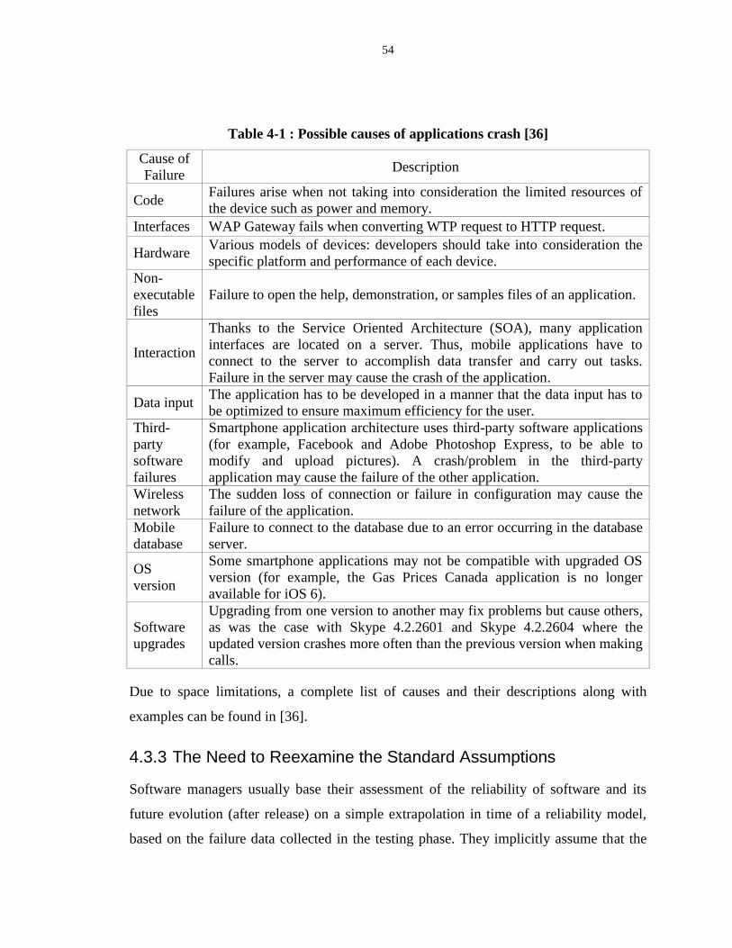
54

Table 4-1 : Possible causes of applications crash [36]

Cause of

Failure Description

Code Failures arise when not taking into consideration the limited resources of

the device such as power and memory.

Interfaces WAP Gateway fails when converting WTP request to HTTP request.

Hardware Various models of devices: developers should take into consideration the

specific platform and performance of each device.

Non-

executable

files

Failure to open the help, demonstration, or samples files of an application.

Interaction

Thanks to the Service Oriented Architecture (SOA), many application

interfaces are located on a server. Thus, mobile applications have to

connect to the server to accomplish data transfer and carry out tasks.

Failure in the server may cause the crash of the application.

Data input The application has to be developed in a manner that the data input has to

be optimized to ensure maximum efficiency for the user.

Third-

party

software

failures

Smartphone application architecture uses third-party software applications

(for example, Facebook and Adobe Photoshop Express, to be able to

modify and upload pictures). A crash/problem in the third-party

application may cause the failure of the other application.

Wireless

network

The sudden loss of connection or failure in configuration may cause the

failure of the application.

Mobile

database

Failure to connect to the database due to an error occurring in the database

server.

OS

version

Some smartphone applications may not be compatible with upgraded OS

version (for example, the Gas Prices Canada application is no longer

available for iOS 6).

Software

upgrades

Upgrading from one version to another may fix problems but cause others,

as was the case with Skype 4.2.2601 and Skype 4.2.2604 where the

updated version crashes more often than the previous version when making

calls.

Due to space limitations, a complete list of causes and their descriptions along with

examples can be found in [36].

4.3.3 The Need to Reexamine the Standard Assumptions

Software managers usually base their assessment of the reliability of software and its

future evolution (after release) on a simple extrapolation in time of a reliability model,

based on the failure data collected in the testing phase. They implicitly assume that the

55

field operational usage of the application will not differ greatly from that of the Lab

testing phase [23, 37]. This is the first standard assumption on which most reliability

models are based. As mentioned previously, this assumption is no more valid in the

mobile area as there is a large variation and uncertainty in the operational profile of

smartphone applications (there are so many possible operational profiles, as there are

millions of users). If an application is used in different environments, its reliability may

be different for each environment [11]. Therefore, the “mobile feature” has to be included

in the initial assumptions of any reliability model suited to the mobile area in order for its

assessments and predictions to be taken seriously, and to be of any help to manager

decisions.

4.4 Summary

Based on different surveys and studies, reliability was identified as one of the most

important quality attribute of the application software. Thus, the reliability of smartphone

applications needs to be assured since everyone is using their own smartphones for daily

life activities and tasks, now more than PCs. Our study confirms that a reliability growth

model adapted to smartphone applications is needed since the traditional reliability

models turned out to be inefficient. This conclusion is based on the experimentation we

carried out with three SRGMs applied to three smartphone application failure data.

Therefore this chapter is a clear-cut answer to the research questions 2 and 3, raised in the

introduction.

To the research question 3: “… how do the existing successful reliability models,

used to assess the desktop/laptops applications, perform when applied to the

mobile area? Will these models still be of useful help to smartphone applications

managers, as they were in the desktop/laptop case? Will there be a need to

change them?” As evidenced in all of the experiments carried out in this chapter,

the answer is that the existing successful reliability models, suited to assess the

desktop/laptops applications, do not equally perform when applied to the mobile

area; they fail to reproduce the observed failure data adequately. Therefore, they

need to be changed and adapted to the mobile area.

56

To the research question 2: “Are the basic assumptions needed to build the

reliability models suited to desktop/laptop applications still valid in the case of

smartphone applications? How do we adapt them to the mobile area? ” as

detailed in Sections 2.4 and 4.3, the answer is that there is a need to change the

assumptions on which these models are based, particularly, to adapt them to the

mobile area, these assumptions should be complemented by including the “mobile

feature” reflected in the inherent uncertainties and dynamic operational profiles of

mobile applications, in contrast to the stationary operational profiles of

desktop/laptop applications. This “mobile feature” is application-dependent and

cannot be the same for all smartphone applications.

After realizing the failure of the above mentioned SRGMs to adequately reproduce the

smartphone failure data, in the next chapter we use and compare two common

distributions, Weibull and Gamma, to model new collected failure data of the same

applications, after sorting it by version number and grouping it into different time

periods.

57

Chapter 5

5 Failure Data Analysis of Smartphone Applications Using the Weibull and Gamma Distributions

The preceding chapter was devoted to the application of three most used SRGMs to two

common smartphone applications, Skype and Vtok, and one private Windows phone

application. The inputs to these models were the instantaneous failure data (the failure

number and its exact occurrence time). Those models failed to adequately describe the

failure data. One possible reason is that on a real time scale, the failure data of

smartphone applications are highly fluctuating. Having tried several non-linear regression

models to better fit the failure data and after numerous experiments, we found that

Weibull and Gamma distributions [38, 39] can be used to model new collected failure

data of the same applications, after sorting them by version number and grouping them

into different time periods. Therefore, we used the two mentioned distributions and their

particular cases, the Rayleigh (the particular case of Weibull) and the S-Shaped (the

particular case of Gamma) models and compared their performances for each application.

This study is carried out after two steps: (i) the failure data for each application are sorted

by version number (ii) the data are grouped on larger time scales (days, weeks and

months). A by-product of this approach is an estimation of the total number of defects in

each smartphone application version.

The chapter is organized as follows: Section 5.1 describes the experiments, Section 5.2 is

a brief presentation of the Weibull distribution and its particular case, the Rayleigh

distribution, and Section 5.3 presents the Gamma distribution and its particular case,

called the S-Shaped distribution. Section 5.4 recalls the used evaluation criteria and

Section 5.5 presents the results of the proposed approach and their discussion. Section 5.6

is reserved for the threats to validity issues and a summary is given in Section 5.7.

5.1 Experiments

As several users from many regions had responded to our call for failure data collection

of smartphone applications, we obtained new enriched data for Skype and Vtok

applications. The data are collected synchronously and come from different versions of

58

the applications. When we plot the raw data on the real timescale, the obtained curves are

highly fluctuating and no regularity can be detected. But, after sorting the data by version

number and grouping the data using a larger time scale (days, weeks, months), the

relationship between failure counts and time (days, weeks, months) was represented by a

non-linear graph. After testing several non-linear models, we concluded that the failure

counts present shapes reminiscent of the Weibull or the Gamma distributions: each

application version shows an early “burst of failures” followed by a decrease, where the

failures become less and less frequent. For the Windows phone application, we saw in the

preceding chapter that the failure count curve was highly fluctuating (Figure 4-3), but

when plotted with larger time periods, it also represents the Weibull shape.

Based on this observation, we conducted a thorough study of the collected data. Each

version of each application is studied separately, if there was sufficient data. The versions

with very few failure data are not considered, and they are evidently the most stable. For

the Skype application we collected enough data for three versions, whereas for Vtok we

collected enough data for two versions. For the Windows phone application, we simply

grouped the failure data in larger time scales and modeled the failure count curves.

We present in the following sections, a brief presentation of the Weibull and the Gamma

distributions, and their applications to the modeling of the observed failure data grouped,

as previously indicated. A comparison between the models was carried out in each case,

based on the error criteria. As the Rayleigh and S-shaped models are particular cases of

the Weibull and Gamma distributions respectively, and as they are often used in many

reliability investigations, we also included them in the comparison.

5.2 The Weibull Distribution

The Weibull distribution [38] is a two parameter function whose expression is given by:

b 1 bb t t

f t wblpdf t ,a,b * expa a a

(5.1)

The parameters and take positive values as well as the variable t. If we define

and , this expression simplifies to:

59

B 1 Bf t B A t  exp A t  (5.2)

For b = 1, this function reduces to the exponential function, whereas for b = 2, it reduces

to the Rayleigh function.

A maximum for this function occurs at time , such that

b

max

B 1T  

A B

(5.3)

or using the a, b notation is such that:

b b

max

b 1T  a  

 b

(5.4)

The cumulative distribution function associated with the Weibull distribution is given by:

bF t 1 exp A t  (5.5)

The failure count at time t is written as:

B 1 By t C f t C B A t  exp A t  (5.6)

and the cumulative failure number by time t is given by:

bY t    C F t C 1 exp A t  (5.7)

where the parameter C is the total number of expected failures: .

Therefore the cumulative number of observed failures by time is:

max max

B 1Y  t T    C F  t T C  1 exp

B

(5.8)

60

The famous 40% rule for the Rayleigh distribution is obtained from the preceding

equation when B = 2: the fraction (or the proportion) of failures, observed by time

is given by:

maxY  t T 2 11 exp 0.3934 ~ 40%

2C

(5.9)

5.3 The Gamma Distribution

The Gamma distribution [39] is a two parameter function whose expression is given by:

a 1

a

1 tf t gampdf t ,a,b t exp

b Γ a b

(5.10)

a 11 t t

f t gampdf t ,a,b expb Γ a b b

(5.11)

for , , and t taking positive values. For a = 1, this function reduces to the exponential

distribution. The maximum of this function occurs at such that:

max T b  a 1 (5.12)

The cumulative distribution function associated with the Gamma distribution is given by:

t

0

tγ a,

bF t f t dt

Γ a

(5.13)

where

is the incomplete Gamma function, being the complete Gamma

function. When , (

) and , as expected.

The failure count at time t is written as:

61

a 1C t t

y t C f t expb Γ a b b

(5.14)

and the cumulative failure number by time t is given by:

tγ a,

bY t    C F t C 

Γ a

(5.15)

where the parameter C is the total number of expected failures.

Therefore the cumulative number of observed failures by time is:

max

max max

     T    γ a,

bY  t T    C F  t T C

Γ a

(5.16)

The relative proportion of failures encountered by time is, in Matlab notation:

max

max max

 Tγ a,

Y  t T  Tb    Gammainc    ,  a

C Γ a b

(5.17)

and for the case of the S-shaped model distribution, it reduces to:

maxY  t T

Gammainc 1   ,  2 26.4%C

(5.18)

because a = 2 and therefore . This is in fact an attractive result

because it is valid for all applications and for all of their versions.

5.4 Evaluation Criteria

For each application, the four used distributions are compared on the basis of their Root-

Mean-Squared-Error (RMSE) and their Adjusted R-Square. The results of the estimated

total number of defects will be evaluated using the Magnitude of Relative Error (MRE).

1. Root Mean Squared Error: the RMSE is the square root of the mean of the square

of the differences between the actual and the predicted values and is expressed as:

62

2

i   i

1

 yRMSE

N

N

i

y

(5.19)

where and are the actual and predicted number of failures respectively, N is the

number of observations.

2. The Magnitude of Relative Error (MRE) for each observation i can be obtained as

follows :

C  C

MREC

ˆ (5.20)

where and are the actual and predicted cumulative number of failures respectively.

3. The adjusted R-square: measures the proportion of the variation in the dependent

variable accounted for by the explanatory variables. Unlike R square, adjusted R

square allows for the degrees of freedom associated with the sums of the squares.

Therefore, even though the residual sum of squares decreases or remains the same

as new explanatory variables are added, the residual variance does not. For this

reason, adjusted R square is generally considered to be a more accurate goodness-

of-fit measure than R square. The adjusted R-square can be negative [40].

5.5 Results

This section presents a comparison and evaluation of the use of the above mentioned

distributions to model the failure data of three versions of Skype, two versions of Vtok,

and the Windows phone application, based on the evaluation criteria explained above.

5.5.1 Skype Application

The accumulated failure data from the Skype application were sorted by version number,

and sufficient failure data for three different versions were collected. They will be called

in the following: Skype Version 1, 2, and 3. Skype Version 2 follows Skype Version 1

chronologically.

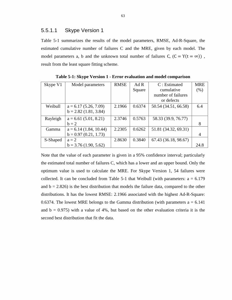
63

5.5.1.1 Skype Version 1

Table 5-1 summarizes the results of the model parameters, RMSE, Ad-R-Square, the

estimated cumulative number of failures C and the MRE, given by each model. The

model parameters a, b and the unknown total number of failures ( ,

result from the least square fitting scheme.

Table 5-1: Skype Version 1 - Error evaluation and model comparison

Skype V1 Model parameters RMSE Ad R

Square

C : Estimated

cumulative

number of failures

or defects

MRE

(%)

Weibull a = 6.17 (5.26, 7.09)

b = 2.82 (1.81, 3.84)

2.1966 0.6374 50.54 (34.51, 66.58) 6.4

Rayleigh a = 6.61 (5.01, 8.21)

b = 2

2.3746 0.5763 58.33 (39.9, 76.77)

8

Gamma a = 6.14 (1.84, 10.44)

b = 0.97 (0.21, 1.73)

2.2305 0.6262 51.81 (34.32, 69.31)

4

S-Shaped a = 2

b = 3.76 (1.90, 5.62)

2.8630 0.3840 67.43 (36.18, 98.67)

24.8

Note that the value of each parameter is given in a 95% confidence interval; particularly

the estimated total number of failures C, which has a lower and an upper bound. Only the

optimum value is used to calculate the MRE. For Skype Version 1, 54 failures were

collected. It can be concluded from Table 5-1 that Weibull (with parameters: a = 6.179

and b = 2.826) is the best distribution that models the failure data, compared to the other

distributions. It has the lowest RMSE: 2.1966 associated with the highest Ad-R-Square:

0.6374. The lowest MRE belongs to the Gamma distribution (with parameters a = 6.141

and b = 0.975) with a value of 4%, but based on the other evaluation criteria it is the

second best distribution that fit the data.

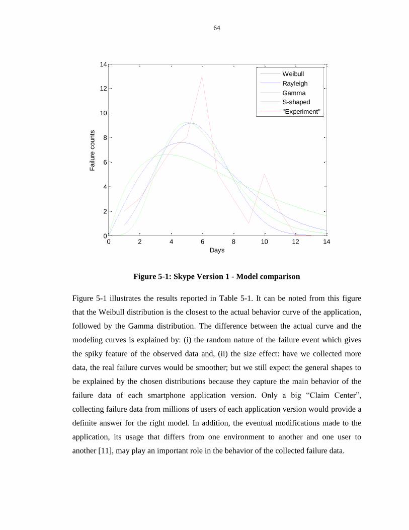
64

Figure 5-1: Skype Version 1 - Model comparison

Figure 5-1 illustrates the results reported in Table 5-1. It can be noted from this figure

that the Weibull distribution is the closest to the actual behavior curve of the application,

followed by the Gamma distribution. The difference between the actual curve and the

modeling curves is explained by: (i) the random nature of the failure event which gives

the spiky feature of the observed data and, (ii) the size effect: have we collected more

data, the real failure curves would be smoother; but we still expect the general shapes to

be explained by the chosen distributions because they capture the main behavior of the

failure data of each smartphone application version. Only a big “Claim Center”,

collecting failure data from millions of users of each application version would provide a

definite answer for the right model. In addition, the eventual modifications made to the

application, its usage that differs from one environment to another and one user to

another [11], may play an important role in the behavior of the collected failure data.

0 2 4 6 8 10 12 140

2

4

6

8

10

12

14

Days

Failu

re c

ounts

Weibull

Rayleigh

Gamma

S-shaped

"Experiment"

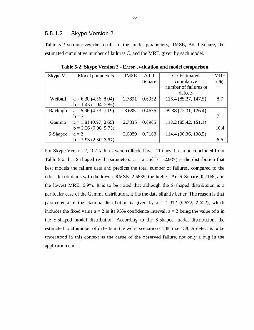
65

5.5.1.2 Skype Version 2

Table 5-2 summarizes the results of the model parameters, RMSE, Ad-R-Square, the

estimated cumulative number of failures C, and the MRE, given by each model.

Table 5-2: Skype Version 2 - Error evaluation and model comparison

Skype V2 Model parameters RMSE Ad R

Square

C : Estimated

cumulative

number of failures or

defects

MRE

(%)

Weibull a = 6.30 (4.56, 8.04)

b = 1.45 (1.04, 2.86)

2.7891 0.6952 116.4 (85.27, 147.5) 8.7

Rayleigh a = 5.96 (4.73, 7.19)

b = 2

3.685 0.4676 99.38 (72.31, 126.4)

7.1

Gamma a = 1.81 (0.97, 2.65)

b = 3.36 (0.98, 5.75)

2.7835 0.6965 118.2 (85.42, 151.1)

10.4

S-Shaped a = 2

b = 2.93 (2.30, 3.57)

2.6889 0.7168 114.4 (90.36, 138.5)

6.9

For Skype Version 2, 107 failures were collected over 11 days. It can be concluded from

Table 5-2 that S-shaped (with parameters: a = 2 and b = 2.937) is the distribution that

best models the failure data and predicts the total number of failures, compared to the

other distributions with the lowest RMSE: 2.6889, the highest Ad-R-Square: 0.7168, and

the lowest MRE: 6.9%. It is to be noted that although the S-shaped distribution is a

particular case of the Gamma distribution, it fits the data slightly better. The reason is that

parameter a of the Gamma distribution is given by a = 1.812 (0.972, 2.652), which

includes the fixed value a = 2 in its 95% confidence interval, a = 2 being the value of a in

the S-shaped model distribution. According to the S-shaped model distribution, the

estimated total number of defects in the worst scenario is 138.5 i.e.139. A defect is to be

understood in this context as the cause of the observed failure, not only a bug in the

application code.

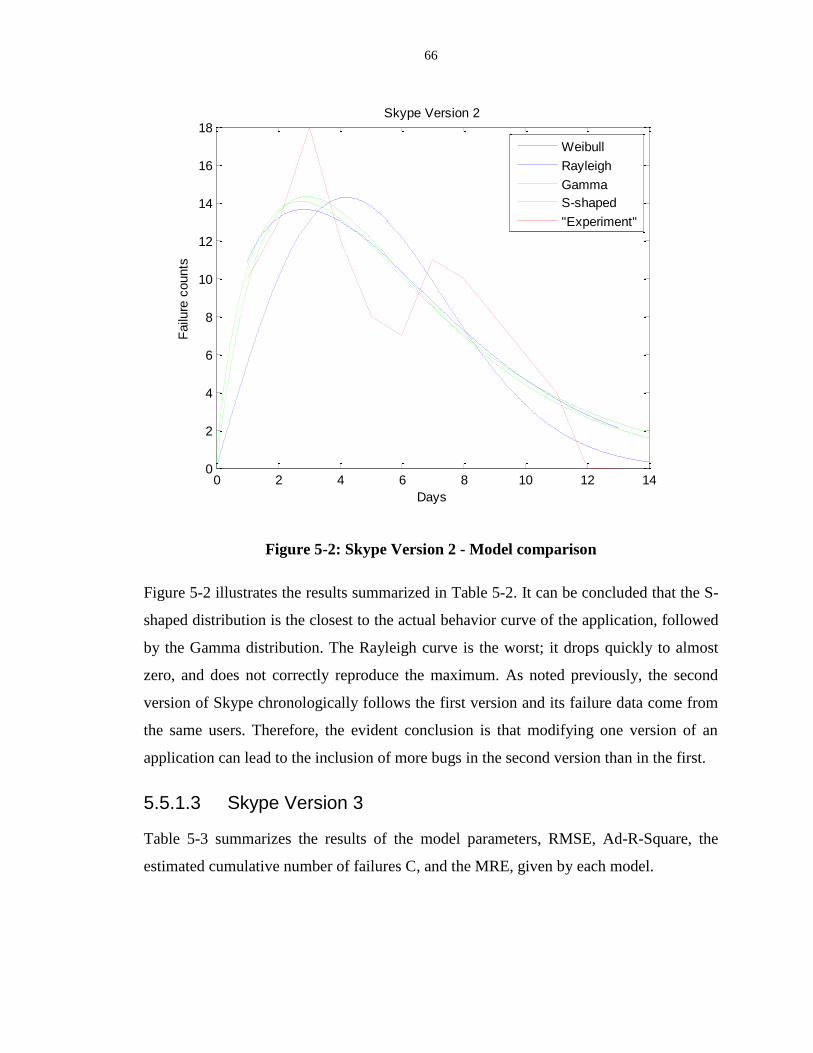
66

Figure 5-2: Skype Version 2 - Model comparison

Figure 5-2 illustrates the results summarized in Table 5-2. It can be concluded that the S-

shaped distribution is the closest to the actual behavior curve of the application, followed

by the Gamma distribution. The Rayleigh curve is the worst; it drops quickly to almost

zero, and does not correctly reproduce the maximum. As noted previously, the second

version of Skype chronologically follows the first version and its failure data come from

the same users. Therefore, the evident conclusion is that modifying one version of an

application can lead to the inclusion of more bugs in the second version than in the first.

5.5.1.3 Skype Version 3

Table 5-3 summarizes the results of the model parameters, RMSE, Ad-R-Square, the

estimated cumulative number of failures C, and the MRE, given by each model.

0 2 4 6 8 10 12 140

2

4

6

8

10

12

14

16

18

Days

Failu

re c

ounts

Skype Version 2

Weibull

Rayleigh

Gamma

S-shaped

"Experiment"

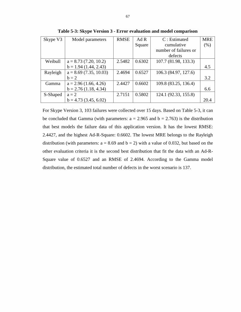
67

Table 5-3: Skype Version 3 - Error evaluation and model comparison

Skype V3 Model parameters RMSE Ad R

Square

C : Estimated

cumulative

number of failures or

defects

MRE

(%)

Weibull a = 8.73 (7.20, 10.2)

b = 1.94 (1.44, 2.43)

2.5482 0.6302 107.7 (81.98, 133.3)

4.5

Rayleigh a = 8.69 (7.35, 10.03)

b = 2

2.4694 0.6527 106.3 (84.97, 127.6)

3.2

Gamma a = 2.96 (1.66, 4.26)

b = 2.76 (1.18, 4.34)

2.4427 0.6602 109.8 (83.25, 136.4)

6.6

S-Shaped a = 2

b = 4.73 (3.45, 6.02)

2.7151 0.5802 124.1 (92.33, 155.8)

20.4

For Skype Version 3, 103 failures were collected over 15 days. Based on Table 5-3, it can

be concluded that Gamma (with parameters: a = 2.965 and b = 2.763) is the distribution

that best models the failure data of this application version. It has the lowest RMSE:

2.4427, and the highest Ad-R-Square: 0.6602. The lowest MRE belongs to the Rayleigh

distribution (with parameters: a = 8.69 and b = 2) with a value of 0.032, but based on the

other evaluation criteria it is the second best distribution that fit the data with an Ad-R-

Square value of 0.6527 and an RMSE of 2.4694. According to the Gamma model

distribution, the estimated total number of defects in the worst scenario is 137.

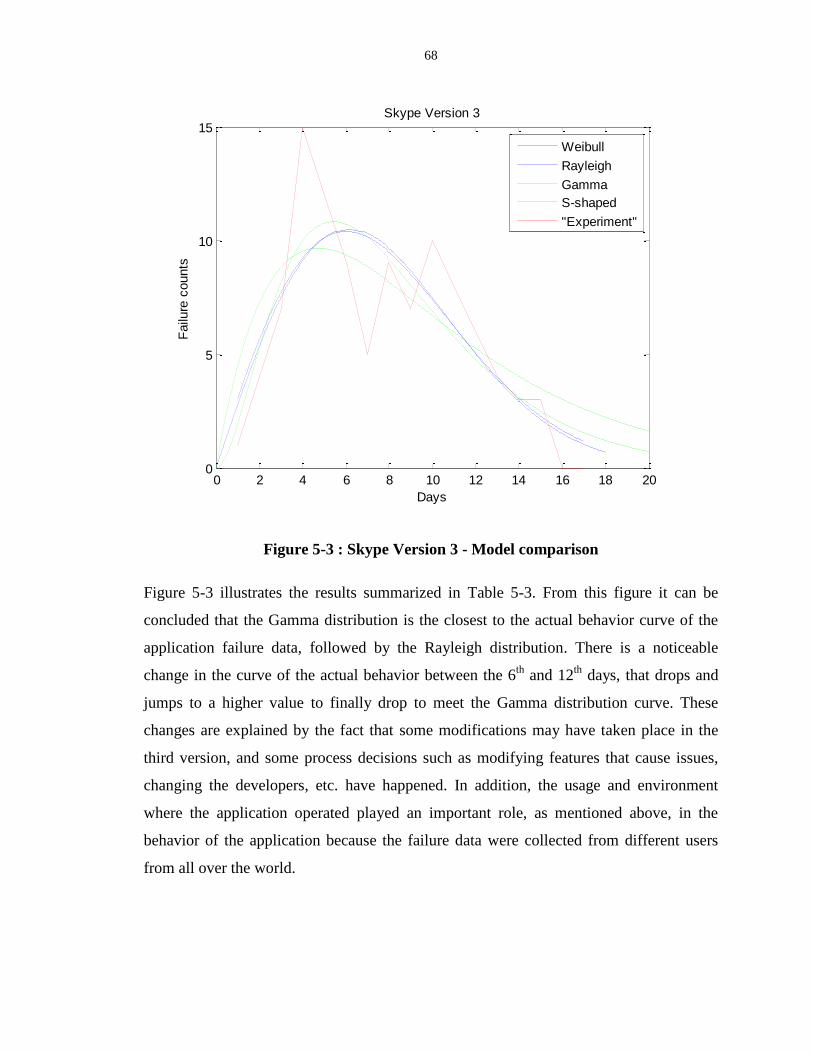
68

Figure 5-3 : Skype Version 3 - Model comparison

Figure 5-3 illustrates the results summarized in Table 5-3. From this figure it can be

concluded that the Gamma distribution is the closest to the actual behavior curve of the

application failure data, followed by the Rayleigh distribution. There is a noticeable

change in the curve of the actual behavior between the 6th

and 12th

days, that drops and

jumps to a higher value to finally drop to meet the Gamma distribution curve. These

changes are explained by the fact that some modifications may have taken place in the

third version, and some process decisions such as modifying features that cause issues,

changing the developers, etc. have happened. In addition, the usage and environment

where the application operated played an important role, as mentioned above, in the

behavior of the application because the failure data were collected from different users

from all over the world.

0 2 4 6 8 10 12 14 16 18 200

5

10

15

Days

Failu

re c

ounts

Skype Version 3

Weibull

Rayleigh

Gamma

S-shaped

"Experiment"

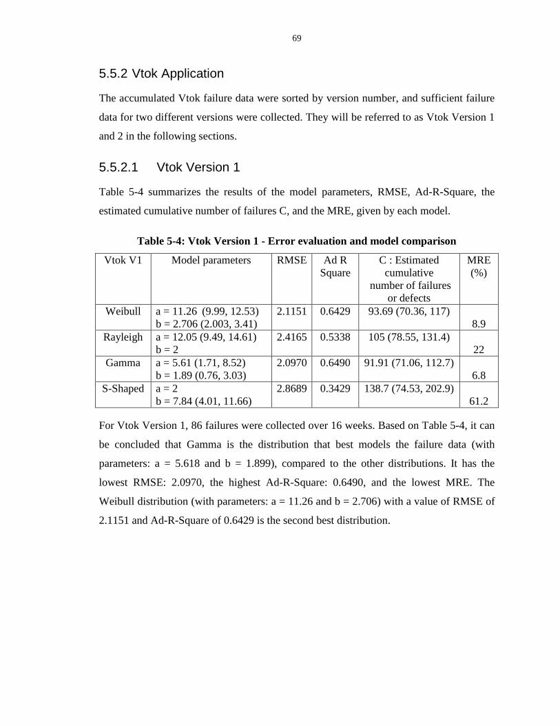
69

5.5.2 Vtok Application

The accumulated Vtok failure data were sorted by version number, and sufficient failure

data for two different versions were collected. They will be referred to as Vtok Version 1

and 2 in the following sections.

5.5.2.1 Vtok Version 1

Table 5-4 summarizes the results of the model parameters, RMSE, Ad-R-Square, the

estimated cumulative number of failures C, and the MRE, given by each model.

Table 5-4: Vtok Version 1 - Error evaluation and model comparison

Vtok V1 Model parameters RMSE Ad R

Square

C : Estimated

cumulative

number of failures

or defects

MRE

(%)

Weibull a = 11.26 (9.99, 12.53)

b = 2.706 (2.003, 3.41)

2.1151 0.6429 93.69 (70.36, 117)

8.9

Rayleigh a = 12.05 (9.49, 14.61)

b = 2

2.4165 0.5338 105 (78.55, 131.4)

22

Gamma a = 5.61 (1.71, 8.52)

b = 1.89 (0.76, 3.03)

2.0970 0.6490 91.91 (71.06, 112.7)

6.8

S-Shaped a = 2

b = 7.84 (4.01, 11.66)

2.8689 0.3429 138.7 (74.53, 202.9)

61.2

For Vtok Version 1, 86 failures were collected over 16 weeks. Based on Table 5-4, it can

be concluded that Gamma is the distribution that best models the failure data (with

parameters: a = 5.618 and b = 1.899), compared to the other distributions. It has the

lowest RMSE: 2.0970, the highest Ad-R-Square: 0.6490, and the lowest MRE. The

Weibull distribution (with parameters: a = 11.26 and b = 2.706) with a value of RMSE of

2.1151 and Ad-R-Square of 0.6429 is the second best distribution.

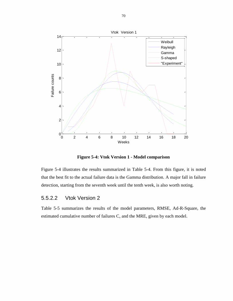
70

Figure 5-4: Vtok Version 1 - Model comparison

Figure 5-4 illustrates the results summarized in Table 5-4. From this figure, it is noted

that the best fit to the actual failure data is the Gamma distribution. A major fall in failure

detection, starting from the seventh week until the tenth week, is also worth noting.

5.5.2.2 Vtok Version 2

Table 5-5 summarizes the results of the model parameters, RMSE, Ad-R-Square, the

estimated cumulative number of failures C, and the MRE, given by each model.

0 2 4 6 8 10 12 14 16 18 200

2

4

6

8

10

12

14

Weeks

Failu

re c

ounts

Vtok Version 1

Weibull

Rayleigh

Gamma

S-shaped

"Experiment"

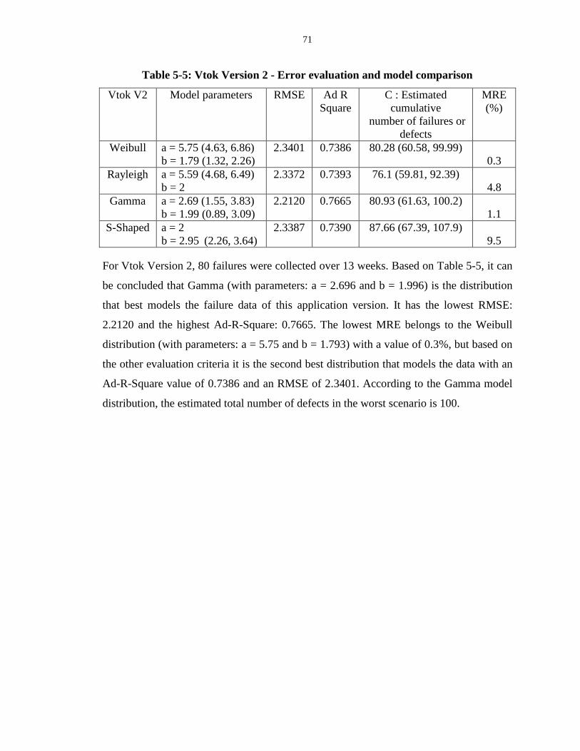
71

Table 5-5: Vtok Version 2 - Error evaluation and model comparison

Vtok V2 Model parameters RMSE Ad R

Square

C : Estimated

cumulative

number of failures or

defects

MRE

(%)

Weibull a = 5.75 (4.63, 6.86)

b = 1.79 (1.32, 2.26)

2.3401 0.7386 80.28 (60.58, 99.99)

0.3

Rayleigh a = 5.59 (4.68, 6.49)

b = 2

2.3372 0.7393 76.1 (59.81, 92.39) 4.8

Gamma a = 2.69 (1.55, 3.83)

b = 1.99 (0.89, 3.09)

2.2120 0.7665 80.93 (61.63, 100.2)

1.1

S-Shaped a = 2

b = 2.95 (2.26, 3.64)

2.3387 0.7390 87.66 (67.39, 107.9)

9.5

For Vtok Version 2, 80 failures were collected over 13 weeks. Based on Table 5-5, it can

be concluded that Gamma (with parameters: a = 2.696 and b = 1.996) is the distribution

that best models the failure data of this application version. It has the lowest RMSE:

2.2120 and the highest Ad-R-Square: 0.7665. The lowest MRE belongs to the Weibull

distribution (with parameters: a = 5.75 and b = 1.793) with a value of 0.3%, but based on

the other evaluation criteria it is the second best distribution that models the data with an

Ad-R-Square value of 0.7386 and an RMSE of 2.3401. According to the Gamma model

distribution, the estimated total number of defects in the worst scenario is 100.

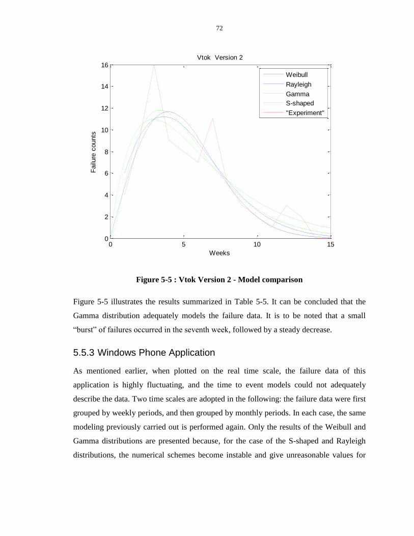
72

Figure 5-5 : Vtok Version 2 - Model comparison

Figure 5-5 illustrates the results summarized in Table 5-5. It can be concluded that the

Gamma distribution adequately models the failure data. It is to be noted that a small

“burst” of failures occurred in the seventh week, followed by a steady decrease.

5.5.3 Windows Phone Application

As mentioned earlier, when plotted on the real time scale, the failure data of this

application is highly fluctuating, and the time to event models could not adequately

describe the data. Two time scales are adopted in the following: the failure data were first

grouped by weekly periods, and then grouped by monthly periods. In each case, the same

modeling previously carried out is performed again. Only the results of the Weibull and

Gamma distributions are presented because, for the case of the S-shaped and Rayleigh

distributions, the numerical schemes become instable and give unreasonable values for

0 5 10 150

2

4

6

8

10

12

14

16

Weeks

Failu

re c

ounts

Vtok Version 2

Weibull

Rayleigh

Gamma

S-shaped

"Experiment"

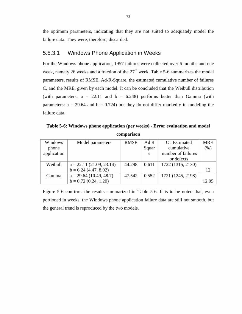
73

the optimum parameters, indicating that they are not suited to adequately model the

failure data. They were, therefore, discarded.

5.5.3.1 Windows Phone Application in Weeks

For the Windows phone application, 1957 failures were collected over 6 months and one

week, namely 26 weeks and a fraction of the 27th

week. Table 5-6 summarizes the model

parameters, results of RMSE, Ad-R-Square, the estimated cumulative number of failures

C, and the MRE, given by each model. It can be concluded that the Weibull distribution

(with parameters: a = 22.11 and b = 6.248) performs better than Gamma (with

parameters: a = 29.64 and b = 0.724) but they do not differ markedly in modeling the

failure data.

Table 5-6: Windows phone application (per weeks) - Error evaluation and model

comparison

Windows

phone

application

Model parameters RMSE Ad R

Squar

e

C : Estimated

cumulative

number of failures

or defects

MRE

(%)

Weibull a = 22.11 (21.09, 23.14)

b = 6.24 (4.47, 8.02)

44.298 0.611 1722 (1315, 2130)

12

Gamma a = 29.64 (10.49, 48.7)

b = 0.72 (0.24, 1.20)

47.542 0.552 1721 (1245, 2198)

12.05

Figure 5-6 confirms the results summarized in Table 5-6. It is to be noted that, even

portioned in weeks, the Windows phone application failure data are still not smooth, but

the general trend is reproduced by the two models.

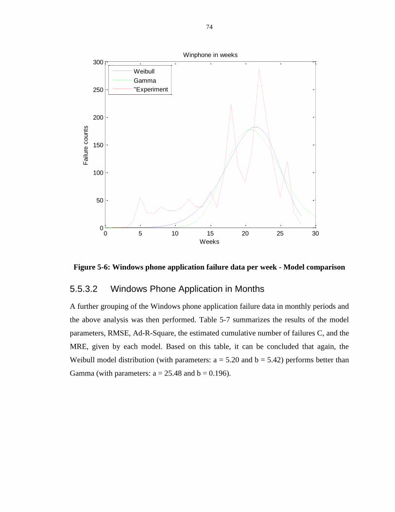
74

Figure 5-6: Windows phone application failure data per week - Model comparison

5.5.3.2 Windows Phone Application in Months

A further grouping of the Windows phone application failure data in monthly periods and

the above analysis was then performed. Table 5-7 summarizes the results of the model

parameters, RMSE, Ad-R-Square, the estimated cumulative number of failures C, and the

MRE, given by each model. Based on this table, it can be concluded that again, the

Weibull model distribution (with parameters: a = 5.20 and b = 5.42) performs better than

Gamma (with parameters: a = 25.48 and b = 0.196).

0 5 10 15 20 25 300

50

100

150

200

250

300

Weeks

Failu

re c

ounts

Winphone in weeks

Weibull

Gamma

"Experiment

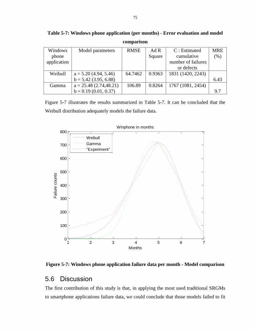
75

Table 5-7: Windows phone application (per months) - Error evaluation and model

comparison

Windows

phone

application

Model parameters RMSE Ad R

Square

C : Estimated

cumulative

number of failures

or defects

MRE

(%)

Weibull a = 5.20 (4.94, 5.46)

b = 5.42 (3.95, 6.88)

64.7462 0.9363 1831 (1420, 2243)

6.43

Gamma a = 25.48 (2.74,48.21)

b = 0.19 (0.01, 0.37)

106.89 0.8264 1767 (1081, 2454)

9.7

Figure 5-7 illustrates the results summarized in Table 5-7. It can be concluded that the

Weibull distribution adequately models the failure data.

Figure 5-7: Windows phone application failure data per month - Model comparison

5.6 Discussion

The first contribution of this study is that, in applying the most used traditional SRGMs

to smartphone applications failure data, we could conclude that those models failed to fit

1 2 3 4 5 6 70

100

200

300

400

500

600

700

800

Months

Failu

re c

ounts

Winphone in months

Weibull

Gamma

"Experiment"

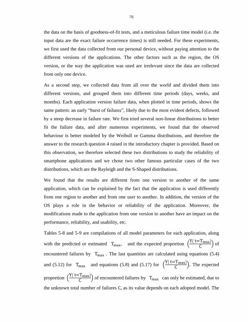
76

the data on the basis of goodness-of-fit tests, and a meticulous failure time model (i.e. the

input data are the exact failure occurrence times) is still needed. For these experiments,

we first used the data collected from our personal device, without paying attention to the

different versions of the applications. The other factors such as the region, the OS

version, or the way the application was used are irrelevant since the data are collected

from only one device.

As a second step, we collected data from all over the world and divided them into

different versions, and grouped them into different time periods (days, weeks, and

months). Each application version failure data, when plotted in time periods, shows the

same pattern: an early “burst of failures”, likely due to the most evident defects, followed

by a steep decrease in failure rate. We first tried several non-linear distributions to better

fit the failure data, and after numerous experiments, we found that the observed

behaviour is better modeled by the Weibull or Gamma distributions, and therefore the

answer to the research question 4 raised in the introductory chapter is provided. Based on

this observation, we therefore selected these two distributions to study the reliability of

smartphone applications and we chose two other famous particular cases of the two

distributions, which are the Rayleigh and the S-Shaped distributions.

We found that the results are different from one version to another of the same

application, which can be explained by the fact that the application is used differently

from one region to another and from one user to another. In addition, the version of the

OS plays a role in the behavior or reliability of the application. Moreover, the

modifications made to the application from one version to another have an impact on the

performance, reliability, and usability, etc.

Tables 5-8 and 5-9 are compilations of all model parameters for each application, along

with the predicted or estimated , and the expected proportion ( ( )

) of

encountered failures by . The last quantities are calculated using equations (5.4)

and (5.12) for and equations (5.8) and (5.17) for ( ( )

). The expected

proportion ( ( )

) of encountered failures by can only be estimated, due to

the unknown total number of failures , as its value depends on each adopted model. The

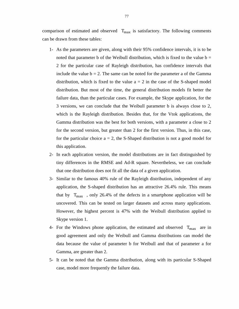
77

comparison of estimated and observed is satisfactory. The following comments

can be drawn from these tables:

1- As the parameters are given, along with their 95% confidence intervals, it is to be

noted that parameter b of the Weibull distribution, which is fixed to the value b =

2 for the particular case of Rayleigh distribution, has confidence intervals that

include the value b = 2. The same can be noted for the parameter a of the Gamma

distribution, which is fixed to the value a = 2 in the case of the S-shaped model

distribution. But most of the time, the general distribution models fit better the

failure data, than the particular cases. For example, the Skype application, for the

3 versions, we can conclude that the Weibull parameter b is always close to 2,

which is the Rayleigh distribution. Besides that, for the Vtok applications, the

Gamma distribution was the best for both versions, with a parameter a close to 2

for the second version, but greater than 2 for the first version. Thus, in this case,

for the particular choice a = 2, the S-Shaped distribution is not a good model for

this application.

2- In each application version, the model distributions are in fact distinguished by

tiny differences in the RMSE and Ad-R square. Nevertheless, we can conclude

that one distribution does not fit all the data of a given application.

3- Similar to the famous 40% rule of the Rayleigh distribution, independent of any

application, the S-shaped distribution has an attractive 26.4% rule. This means

that by , only 26.4% of the defects in a smartphone application will be

uncovered. This can be tested on larger datasets and across many applications.

However, the highest percent is 47% with the Weibull distribution applied to

Skype version 1.

4- For the Windows phone application, the estimated and observed are in

good agreement and only the Weibull and Gamma distributions can model the

data because the value of parameter b for Weibull and that of parameter a for

Gamma, are greater than 2.

5- It can be noted that the Gamma distribution, along with its particular S-Shaped

case, model more frequently the failure data.

78

Table 5-8: Skype - The parameter values of the model distributions

Skype Version 1 Skype Version 2 Skype Version 3

Weibull a = 6.179 (5.262, 7.096)

b = 2.826 (1.811, 3.84)

c = 50.54 (34.51, 66.58)

observed = 6

Estimated = 5.98

Estimated

(

) 47%

a = 6.305 (4.564,

8.046)

b = 1.457 (1.047,

2.866)

c = 116.4 (85.27,

147.5)

observed = 3

Estimated = 2.84

Estimated

(

)

a = 8.734 (7.201,

10.27)

b = 1.941 (1.447,

2.436)

c = 107.7 (81.98,

133.3)

observed = 4

Estimated = 6.04

Estimated

(

)

Rayleigh a = 6.618 (5.017, 8.218)

b = 2

c = 58.33 (39.9, 76.77)

observed = 6

Estimated = 4.68

Estimated

(

)

40%

a = 5.965 (4.733,

7.196)

b = 2

c = 99.38 (72.31,

126.4)

observed = 3

Estimated = 4.21

Estimated

(

)

a = 8.69 (7.354, 10.03)

b = 2

c = 106.3 (84.97,

127.6)

observed = 4

Estimated = 6.14

Estimated

(

) Gamma a = 6.141 (1.842, 10.44)

b = 0.975 (0.2143,

1.736)

c = 51.81 (34.32,

69.31)

observed = 6

Estimated = 5.01

Estimated

(

) 38.5%

a = 1.812 (0.972,

2.652)

b = 3.366 (0.982, 5.75)

c = 118.2 (85.42,

151.1)

observed = 3

Estimated = 2.73

Estimated

(

)

a = 2.965 (1.662,

4.268)

b = 2.763 (1.184,

4.342)

c = 109.8 (83.25,

136.4)

observed = 4

Estimated = 5.42

Estimated

(

)

S-shaped a = 2

b = 3.767 (1.909, 5.624)

c = 67.43 (36.18, 98.67)

observed = 6

Estimated = 3.76

Estimated

(

)

a = 2

b = 2.937 (2.302,

3.572)

c = 114.4 (90.36,

138.5)

observed = 3

Estimated = 2.93

Estimated

(

)

a = 2

b = 4.738 (3.454,

6.022)

c = 124.1 (92.33,

155.8)

observed = 4

Estimated = 4.73

Estimated

(

)

79

Table 5-9 : Vtok - The parameter values of the model distributions

Vtok Version 1 Vtok Version 2

Weibull a = 11.26 (9.993, 12.53)

b = 2.706 (2.003, 3.41)

c = 93.69 (70.36, 117)

observed = 8

Estimated = 9.40

Estimated (

) 46%

a = 5.75 (4.636, 6.865)

b = 1.793 (1.327, 2.26)

c = 80.28 (60.58, 99.99)

observed = 3

Estimated = 3.64

Estimated (

) 39%

Rayleigh a = 12.05 (9.493, 14.6)

b = 2

c = 105 (78.55, 131.4)

observed = 8

Estimated = 8.52

Estimated (

) 40%

a = 5.592 (4.687, 6.497)

b = 2

c = 76.1 (59.81, 92.39)

observed = 3

Estimated = 3.95

Estimated (

) 40%

Gamma a = 5.618 (1.712, 8.523)

b = 1.899 (0.7642, 3.034)

c = 91.91 (71.06, 112.7)

observed = 8

Estimated = 8.76

Estimated (

) 37.8%

a = 2.696 (1.556, 3.836)

b = 1.996 (0.8937, 3.098)

c = 80.93 (61.63, 100.2)

observed = 3

Estimated = 3.38

Estimated (

)

S-shaped a = 2

b = 7.841 (4.018, 11.66)

c = 138.7 (74.53, 202.9)

observed = 8

Estimated = 7.84

Estimated (

) 26.4%

a = 2

b = 2.953 (2.26, 3.646)

c = 87.66 (67.39, 107.9)

observed = 3

Estimated = 2.95

Estimated (

) 26.4%

80

Table 5-10: Windows phone application - Parameter values of the model

distributions

Windows phone application in weeks Windows phone application in

months

Weibull a = 22.11 (21.09, 23.14)

b = 6.248 (4.474, 8.021)

c = 1722 (1315, 2130)

observed = 22

Estimated = 21.5

Estimated (

) 56.83%

a = 5.204 (4.94, 5.469)

b = 5.42 (3.953, 6.887)

c = 1831 (1420, 2243)

observed = 5

Estimated = 5.01

Estimated (

) 55.76%

Gamma a = 29.64 (10.49, 48.7

b = 0.7247 (0.2417, 1.208)

c = 1721 (1245, 2198)

observed = 22

Estimated = 20.75

Estimated (

) 45%

a = 25.48 (2.743, 48.21)

b = 0.1969 (0.01633, 0.3775)

c = 1767 (1081, 2454)

observed = 5

Estimated = 4.82

Estimated (

) 44.65%

5.7 Threats to Validity:

As studying the reliability of smartphone applications is a new approach and no previous

work or techniques were suggested, some limitations can become a threat to our

approach’s validation, such as:

The data collection was a challenge and not enough data were collected due to

privacy policies from smartphone application developers and friends who

believed that from the crash report of their applications one can control their

phone. Therefore, the limited datasets of our investigation make the generalization

of the results difficult. Moreover, predicting the reliability should be in the

development phase but because of lack of data during this stage, we used the data

collected after release.

Experimentation with more elaborate data and other model distributions can be

investigated.

Data from different platforms, such as Android and its users, will be useful to

obtain more accurate results.

81

The data were collected during the operational phases. Also we do not have an

idea about the early development stages of the application and its architecture as

to whether it is complex or simple. In addition, we do not know how the

application was used and under which conditions. All of these factors may create

more defects than anticipated.

Only a few versions were used in this study, more versions of the applications

would help to provide a better idea as to whether the versions’ failure data are

independent of each other, or correlated in a particular way.

It is not guaranteed that the modifications made to the application from one

version to another would not introduce more bugs or complexity. Moreover, it

cannot be assured that the correction of old bugs would not result in other, newer

bugs.

5.8 Summary

The collected failure data of several smartphone application versions were analyzed using

the two model distributions, Weibull and Gamma, and their particular cases: the Rayleigh

and the S-shaped distributions, respectively. Each model distribution provided an

estimation of the expected cumulative number of failures (or equivalently, the number of

defects) in each smartphone application version. The results show that not only one

distribution is useful for the different versions of the same application, but, based on the

evaluation criteria, one distribution can give a better prediction for one version than when

applied to another. Nevertheless, among the cases studied the Gamma distribution and its

particular case, the S-shaped distribution, are more frequently suited, and seem to

perform better than the Weibull and its particular case, the Rayleigh distribution. Further

investigation with more elaborated failure data basis must be pursued in order to rank the

performances of these two model distributions accurately.

Although the distributions did not perfectly fit the data, they were useful in predicting the

cumulative number of failures at the end of each version, with a calculated error. The

40% rule, issued from the Rayleigh distribution, often used by software managers to

estimate the residual defects in a desktop application, has been extended to the Weibull

82

and Gamma distributions in the case of smartphone applications. The proposed approach

in this chapter, namely the use of distributions to model the collected failure data of a

smartphone application versions, suffers greatly from the above mentioned size effect.

However, we believe that the main behavior of the failure event in smartphone

applications is captured by the chosen distributions.

Concerning research question 4, raised in the introductory chapter: “On a practical basis,

how could a software manager model the daily failure data received from complaining

users of a particular smartphone application to get some insight and understanding that

can help in decisions? Is there a distribution that can model the failure data?”, as

evidenced by all of the experiments carried out in this chapter, the answer is that both the

Weibull and the Gamma distributions can be used adequately to model the failure data of

an application by sorting this data by application version number and grouping it into

appropriate time periods.

Finally, there still exists the goal, raised in research question 1 in Chapter 1, to come up

with a new time-to-failure model, i.e. taking as input the exact failure occurrence times,

which will assess and predict the reliability of applications implemented in smartphone

devices, or operating under diverse environmental conditions and usage profiles and that

will be of valued help for software managers in the mobile area. This is still an

unanswered question. We believe that this goal cannot be achieved by a simple model

equation, as there are many interacting variables affecting the reliability of a mobile

application such as: the size of the application, its modular structure or complexity, the

hardware limitations of the devices, the severity of the encountered failures, the network

condition, the operating system used, the uncertainty in operational profile, the other

unknown simultaneously running applications, etc. The right approach would have to

take into account of all these interacting factors. Neural networks and fuzzy-logic

simulations would be appropriate for this investigation.

83

Chapter 6

6 Conclusions

This chapter summarizes the conclusions drawn from our research and suggests possible

directions for future work.

The investigation of smartphone application reliability through the use of well-known

available reliability growth models, suited primarily to desktop applications, was twofold:

(i) highlight the versatile nature of mobile applications, their dynamic configuration,

unknown operational profile, and varying execution conditions in contrast to the static

and stable desktop applications, (ii) stress the need for the design of new reliability

models suited for mobile applications, that take into account the inherent versatility of

such applications.

6.1 Conclusions and Perspectives

In order to answer the first research question raised in the introductory chapter, namely,

“…is it possible to build a mathematical model that helps software managers assess and

predict the reliability of applications implemented in smartphone devices and working

under diverse operational environments and usage profiles?” we began by examining the

related question of the applicability of the available desktop/laptop software reliability

models to the case of mobile applications. Therefore, to answer the focused research

question 3, raised in the introduction, namely “… how do the existing successful

reliability models, used to assess the desktop/laptops applications, perform when applied

to the mobile area? Will these models still be of useful help to smartphone applications

managers, as they were in the desktop/laptop case? Will there be a need to change

them?” we selected, as a first step, three of the most used models that are known for their

efficiency in the desktop area: the NHPP, Musa-Basic, and Musa-Okumoto models.

These models, as well as reliability concepts, are presented in Chapter 3. They use as

their input the failure occurrence times. We used two iPhone applications, Skype and

Vtok, used and tested differently in order to evaluate the models under different

conditions, and one Windows phone application that we kept confidential due to the

company’s confidentiality policies. It turned out that none of the selected SRGMs were

84

able to account for the observed failure data satisfactorily. This investigation was carried

out in Chapter 4 and answered this research question.

As each reliability model relies on its assumptions, the failure of a model is an indication

of the inadequacy of its assumptions. This is formulated by research question 2, namely:

“Are the basic assumptions needed to build the reliability models suited to desktop/laptop

applications still valid in the case of smartphone applications? How do we adapt them to

the mobile area? ” and answered in detail in Sections 2.4 and 4.3.

After noting the failure of the above models, the research question 4, namely: “On a

practical basis, how could a software manager model the daily failure data received from

complaining users of a particular smartphone application to get some insight and

understanding that can help in decisions? Is there a distribution that can model the

failure data?” was logically asked. To this end, we tested many non-linear models based

on the nature of the failure data and found that the Weibull and Gamma distributions

were best suited to model the collected failure data of each application, after sorting its

data by application version number and grouping it into different time periods. Chapter 5

was entirely devoted to answering this research question.

Another related question to the above mentioned primary question is whether the

differences in hardware and software between desktops/laptops and smartphone devices,

as well as their highly varying operational conditions, could affect their reliability. This

was detailed in Chapter 2, which has also presented an overview of the mobile world.

Our study also highlighted the causes of the failure of the above models and the need for

a meticulous Software Reliability Growth Model for smartphone applications; this is

because the existing software reliability approaches were developed for traditional

stationary desktop software applications that are static and stable during their execution,

which is not the case for smartphone applications that have unknown operational profiles,

highly dynamic configurations, and changing execution conditions. On a continuous

background, the smartphone failures occur in relatively short bursts, from time to time,

which explain the abrupt changes in the observed cumulative failure data curves. This

particular feature cannot be accommodated by the selected SRGMs. Thus, in order to

evaluate the reliability of smartphone applications, new models, principles, and tools are

85

needed, in order to incorporate the underlying uncertainties of such applications. In an

attempt to make further progress, and assuming the above mentioned uncertainties and

many other unknown factors concerning the hardware and software used by each

application, two common distributions, Weibull and Gamma, were used to model the

collected failure data after sorting it by application version number and grouping into

varying time periods. The main features of the observed failure behavior of these

applications are captured by the two distributions. Nevertheless, due to the lack of

published smartphone failure data for secrecy reasons, we relied on our own limited

resources and, therefore, our approach suffers from the small sizes of the collected failure

data, preventing us from devising a generalization of the obtained results.

6.2 Future Work

An immediate future work will be to focus on analyzing more in depth those selected

(and other) SRGMs, and to attempt to modify the closest one to the data, to then adapt it

to smartphone applications by altering its basic assumptions, taking into account the

“mobile” feature of the applications. Moreover, we will determine if we need to have a

specific model for each type of application, or if one model is applicable to all of the

categories of smartphone applications, taking into consideration the severity of the

failure, the size and the modular complexity of the application, etc. using machine

learning and more advanced algorithms. Successful examples of the application of

machine learning techniques can be found in [43], [44] and [45].

The availability of hundreds of software reliability models makes it difficult for the

software manager to select among them the most adequate to deal with the reliability of a

specific smartphone application. Nevertheless, the selection should be based on simple

criteria such as the “predictive ability” of a model. It is, therefore, our aim to carry out a

comparative study of many existing reliability models applied to numerous smartphone

applications (recent collected data) and to choose the model that gives the least error

across these applications.

Another immediate future work will be to apply the two model distributions, Weibull and

Gamma, to further collected failure data of other applications, and to assess their

respective performances.

86

References

[1] I. Sommerville, "Introduction to software engineering," in Software Engineering, 9th

ed., Pearson Education, Inc., pp. 4-26, 2010.

[2] S. Easterbrook. Bugs in the space program. University of Toronto [Online]. 2005.

Available: http://www.cs.toronto.edu/~sme/presentations/BugsInTheSpaceProgram.pdf.

[3] V. Wadhwani, F. Memon and M. M. Hameed, "Architecture based reliability and

testing estimation for mobile applications," in Wireless Networks, Information Processing

and Systems, D. M. Akbar Hussain, Ed. Springer, pp. 64-75, 2009.

[4] J. D. Musa, Software Reliability Engineering: More Reliable Software, Faster and

Cheaper. Tata McGraw-Hill Education, 2004.

[5] K. Saha Shishir and M. Mohymen. Software reliability prediction. Blekinge Institue of

Technology [Online]. 2012. Available:

http://www.slideshare.net/MirzaMohymen/software-reliability-prediction.

[6] CNCCS. Smartphone malware. CNCCS [Online]. 2011. Available:

http://press.pandasecurity.com/usa/wp-content/uploads/2011/06/CNCCS-Smartphone-

Malware-Full-Report-Translated-06-7-11-FINAL.pdf.

[7] SquareTrade. Smart phone reliability: Apple iPhones with fewest failures, and major

android manufacturers not far behind. SquareTrade [Online]. 2010. Available:

http://www.squaretrade.com/cell-phone-comparison-study-nov-10.

[8] PhysicsWorld. Smartphone eye test for the developing world. The Institute of Physics

[Online]. 2013. Available:

http://physicsworld.com/cws/article/multimedia/2013/apr/18/smartphone-eye-test-for-

the-developing-world.

[9] A. I. Wasserman, "Software engineering issues for mobile application development,"

Proceedings of the FSE/SDP Workshop on Future of Software Engineering Research,

Santa Fe, NM, USA, pp. 397-400, November 2010.

87

[10] U. Perera, "Reliability of mobile phones," in 1995, Proceedings of the Annual

Reliability and Maintainability Symposium. Washington, DC, USA, pp. 33-38, January

1995.

[11] H. Verkasalo, C. López-Nicolás, F. J. Molina-Castillo and H. Bouwman, "Analysis

of users and non-users of smartphone applications," Telematics and Informatics, vol.

27(3), pp. 242-255, 2010.

[12] S. Jang and E. Lee, "Reliable mobile application modeling based on open API,"

Communications in Computer and Information Science, vol. 59, pp. 168-175, 2009.

[13] L. P. POCATILU, "Influencing Factors of Mobile Applications’ Quality Metrics,"

Economy Informatics, pp. 1-4, 2006.

[14] SocialCubix. Mobile app development life cycle. Social Cubix [Online]. 2012.

Available: http://www.socialcubix.com/blog/mobile-app-development-life-cycle.

[15] SocialCubix. Enterprise mobile application development lifecycle. Social Cubix

[Online]. 2012. Available: http://www.socialcubix.com/downloads/enterprise-mobile-

application-development-lifecycle.pdf.

[16] S. Malek, R. Roshandel, D. Kilgore and I. Elhag, "Improving the reliability of

mobile software systems through continuous analysis and proactive reconfiguration,"

Proceedings of the 31st International Conference on Software Engineering-Companion

Volume. ICSE-Companion 2009. Vancouver, BC, Canada, pp. 275-278, May 2009.

[17] M. R. Lyu, "Software reliability engineering: A roadmap," Proceedings of the

Future of Software Engineering, Minneapolis, MN, USA, pp. 153-170, May 2007.

[18] Nielsen. Android most popular operating system in U.S among recent smartphone

buyers. Nielsen Company [Online]. 2010. Available:

http://www.nielsen.com/us/en/newswire/2010/android-most-popular-operating-system-

in-u-s-among-recent-smartphone-buyers.html.

88

[19] S. Abram. Android iPhone Blackberry. Stephen's Lighthouse [Online]. 2010.

Available: http://stephenslighthouse.com/2010/10/13/android-iphone-blackberry-android-

iphone-blackberry/.

[20] eMarketer. Android grabs ever-greater share of smartphone market. eMarketer

[Online]. 2012. Available: http://www.emarketer.com/Article/Android-Grabs-Ever-

Greater-Share-of-Smartphone-Market/1009248.

[21] W. Farr, "Software reliability modeling survey," in Handbook of Software Reliability

Engineering, M. R. Lyu, Ed. Hightstown, NJ, USA, McGraw-Hill, pp. 71-117, 1996.

[22] D. Trindade and Swami Nathan. Failure rate, which one? Sun Microsystems Inc.

[Online]. 2005. Available: http://www.trindade.com/ISMI_FailureRate_92005.pdf.

[23] C. Ramamoorthy and F. B. Bastani, "Software reliability—status and

perspectives," IEEE Transactions on Software Engineering., vol. 8(4), pp. 354-371,

1982.

[24] ReliaSoft. Reliability growth & repairable system data analysis reference. ReliaSoft

[Online]. 2010. Available: http://rga.reliasoft.com/.

[25] R. Lai and M. Garg, "A Detailed Study of NHPP Software Reliability Models,"

Journal of Software, vol. 7(6), pp. 1296-1306, 2012.

[26] I. Traore. Software reliability engineering. University of Victoria [Online].

Available: http://www.ece.uvic.ca/~itraore/seng426-06/notes/qual06-4-4.pdf.

[27] A. B. Nassif, D. Ho and L. F. Capretz, "Towards an early software estimation using

log-linear regression and a multilayer perceptron model," Journal of Systems and

Software, vol. 86(1), pp. 144-160, 2013.

[28] Y. K. Malaiya and J. Denton, "What do the software reliability growth model

parameters represent?" Proceedings of the 8th

International Symposium on Software

Reliability Engineering, Fort Collins, CO, USA, pp. 124-135, November 1997.

89

[29] J. D. Musa, A. Iannino and K. Okumoto, Software Reliability: Measurement,

Prediction, Application. New York, NY, USA, McGraw-Hill, Inc, 1987.

[30] A. B. Nassif, L. F. Capretz and D. Ho, "Software effort estimation in the early stages

of the software life cycle using a cascade correlation neural network model," Proceedings

of the 13th

ACIS International Conference on Software Engineering, Artificial

Intelligence, Networking and Parallel & Distributed Computing (SNPD), Kyoto, Japan,

pp. 589-594. 2012.

[31] A. B. Nassif, L. F. Capretz and D. Ho, "Estimating software effort based on use case

point model using sugeno fuzzy inference system," Proceedings of the 23rd

IEEE

International Conference on Tools with Artificial Intelligence (ICTAI). Boca Raton,

Florida, USA, pp. 393-398, November 2011.

[32] N. Naseri and J. Vazquez, "Software reliability," in Concordia Institute for

Information Systems Engineering, Montreal, Qc, Canada, November, pp. 1-24, 2012.

[33] C. Huang and T. Hung, "Software reliability analysis and assessment using queueing

models with multiple change-points," Computers & Mathematics with Applications, vol.

60(7), pp. 2015-2030, 2010.

[34] SMERFS. Statistical Modeling and Estimation of Reliability Functions for Software.

SMERFS [Online]. 2010. Available: http://www.slingcode.com/smerfs/.

[35] R. Roshandel and S. Malek, "Refining reliability estimation of mobile software

systems," Proceedings of the 1st International Workshop on Software Architectures and

Mobility, Leipzig, Germany, pp. 39-41, May 2008.

[36] A. K. Jha, "A Risk Catalog for Mobile Applications," PhD diss., Florida Institute of

Technology, 2007.

[37] A. Wood, "Software reliability growth models: Assumptions vs. reality,"

Proceedings of the 8th

International Symposium on Software Reliability Engineering,

Albuquerque, NM, USA, pp. 136-141, November 1997.

90

[38] H. Rinne, The Weibull Distribution: A Handbook. Chapman and Hall/CRC, 2010.

[39] G. N. Powell, Handbook of Gender & Work. Sage Publications, 1999.

[40] G. Judge. Adjusted R squared, (R bar squared). University of Portsmouth [Online].

Available: http://judgeg.myweb.port.ac.uk/ECONMET/Rbarsq.pdf.

[41] S. Meskini, A. B. Nassif, and L. F. Capretz, “Reliability Models Applied to Mobile

Applications,” Proceedings of the 7th IEEE International Conference on Software

Security and Reliability Companion, Washington, D.C., IEEE Press, pp. 155-162, June

2013.

[42] S. Meskini, L. F. Capretz, and A. B. Nassif, “Reliability Prediction of Smartphone

Applications Through Their Failure Data Analysis,” 19th IEEE Pacific Rim International

Symposium on Dependable Computing, Vancouver, B.C., accepted, December 2013.

[43] W. L. Du, D. Ho and L. F. Capretz, "Improving Software Effort Estimation Using

Neuro-Fuzzy Model with SEER-SEM," Global Journal of Computer Science and

Technology, vol. 10, no. 12, pp. 52-64, 2010.

[44] X. Huang, D. Ho, J. Ren, and L. F. Capretz, System and Method for Software

Estimation, US Patent # US-7328202-B2, 2008.

[45] X. Huang, J. Ren and L. F. Capretz. A Neuro-Fuzzy Tool for Software Estimation.

Proceedings of the 20th IEEE International Conference on Software Maintenance, pp.

520, 2004.

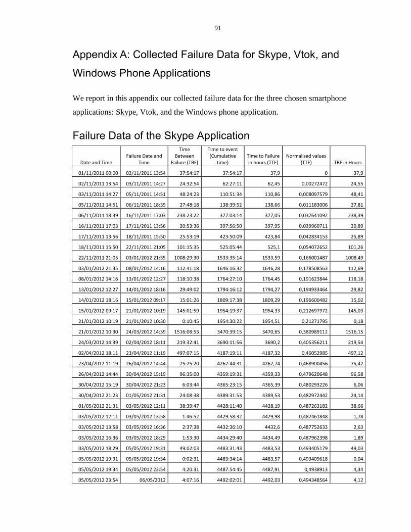
91

Appendix A: Collected Failure Data for Skype, Vtok, and

Windows Phone Applications

We report in this appendix our collected failure data for the three chosen smartphone

applications: Skype, Vtok, and the Windows phone application.

Failure Data of the Skype Application

Date and Time Failure Date and

Time

Time Between

Failure (TBF)

Time to event (Cumulative

time) Time to Failure in hours (TTF)

Normalised values (TTF) TBF in Hours

01/11/2011 00:00 02/11/2011 13:54 37:54:17 37:54:17 37,9 0 37,9

02/11/2011 13:54 03/11/2011 14:27 24:32:54 62:27:11 62,45 0,00272472 24,55

03/11/2011 14:27 05/11/2011 14:51 48:24:23 110:51:34 110,86 0,008097579 48,41

05/11/2011 14:51 06/11/2011 18:39 27:48:18 138:39:52 138,66 0,011183006 27,81

06/11/2011 18:39 16/11/2011 17:03 238:23:22 377:03:14 377,05 0,037641092 238,39

16/11/2011 17:03 17/11/2011 13:56 20:53:36 397:56:50 397,95 0,039960711 20,89

17/11/2011 13:56 18/11/2011 15:50 25:53:19 423:50:09 423,84 0,042834153 25,89

18/11/2011 15:50 22/11/2011 21:05 101:15:35 525:05:44 525,1 0,054072652 101,26

22/11/2011 21:05 03/01/2012 21:35 1008:29:30 1533:35:14 1533,59 0,166001487 1008,49

03/01/2012 21:35 08/01/2012 14:16 112:41:18 1646:16:32 1646,28 0,178508563 112,69

08/01/2012 14:16 13/01/2012 12:27 118:10:38 1764:27:10 1764,45 0,191623844 118,18

13/01/2012 12:27 14/01/2012 18:16 29:49:02 1794:16:12 1794,27 0,194933464 29,82

14/01/2012 18:16 15/01/2012 09:17 15:01:26 1809:17:38 1809,29 0,196600482 15,02

15/01/2012 09:17 21/01/2012 10:19 145:01:59 1954:19:37 1954,33 0,212697972 145,03

21/01/2012 10:19 21/01/2012 10:30 0:10:45 1954:30:22 1954,51 0,21271795 0,18

21/01/2012 10:30 24/03/2012 14:39 1516:08:53 3470:39:15 3470,65 0,380989112 1516,15

24/03/2012 14:39 02/04/2012 18:11 219:32:41 3690:11:56 3690,2 0,405356211 219,54

02/04/2012 18:11 23/04/2012 11:19 497:07:15 4187:19:11 4187,32 0,46052985 497,12

23/04/2012 11:19 26/04/2012 14:44 75:25:20 4262:44:31 4262,74 0,468900456 75,42

26/04/2012 14:44 30/04/2012 15:19 96:35:00 4359:19:31 4359,33 0,479620648 96,58

30/04/2012 15:19 30/04/2012 21:23 6:03:44 4365:23:15 4365,39 0,480293226 6,06

30/04/2012 21:23 01/05/2012 21:31 24:08:38 4389:31:53 4389,53 0,482972442 24,14

01/05/2012 21:31 03/05/2012 12:11 38:39:47 4428:11:40 4428,19 0,487263182 38,66

03/05/2012 12:11 03/05/2012 13:58 1:46:52 4429:58:32 4429,98 0,487461848 1,78

03/05/2012 13:58 03/05/2012 16:36 2:37:38 4432:36:10 4432,6 0,487752633 2,63

03/05/2012 16:36 03/05/2012 18:29 1:53:30 4434:29:40 4434,49 0,487962398 1,89

03/05/2012 18:29 05/05/2012 19:31 49:02:03 4483:31:43 4483,53 0,493405179 49,03

05/05/2012 19:31 05/05/2012 19:34 0:02:31 4483:34:14 4483,57 0,493409618 0,04

05/05/2012 19:34 05/05/2012 23:54 4:20:31 4487:54:45 4487,91 0,4938913 4,34

05/05/2012 23:54 06/05/2012 4:07:16 4492:02:01 4492,03 0,494348564 4,12

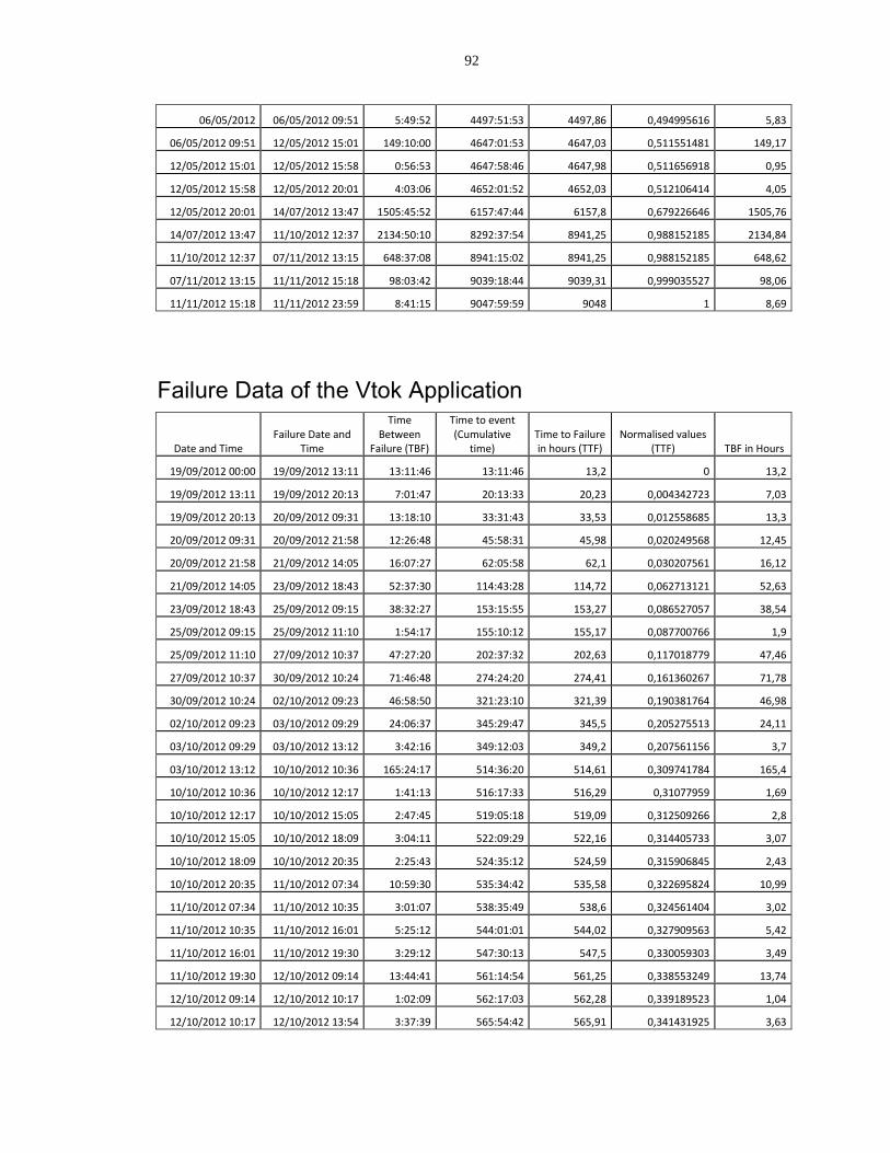
92

06/05/2012 06/05/2012 09:51 5:49:52 4497:51:53 4497,86 0,494995616 5,83

06/05/2012 09:51 12/05/2012 15:01 149:10:00 4647:01:53 4647,03 0,511551481 149,17

12/05/2012 15:01 12/05/2012 15:58 0:56:53 4647:58:46 4647,98 0,511656918 0,95

12/05/2012 15:58 12/05/2012 20:01 4:03:06 4652:01:52 4652,03 0,512106414 4,05

12/05/2012 20:01 14/07/2012 13:47 1505:45:52 6157:47:44 6157,8 0,679226646 1505,76

14/07/2012 13:47 11/10/2012 12:37 2134:50:10 8292:37:54 8941,25 0,988152185 2134,84

11/10/2012 12:37 07/11/2012 13:15 648:37:08 8941:15:02 8941,25 0,988152185 648,62

07/11/2012 13:15 11/11/2012 15:18 98:03:42 9039:18:44 9039,31 0,999035527 98,06

11/11/2012 15:18 11/11/2012 23:59 8:41:15 9047:59:59 9048 1 8,69

Failure Data of the Vtok Application

Date and Time Failure Date and

Time

Time Between

Failure (TBF)

Time to event (Cumulative

time) Time to Failure in hours (TTF)

Normalised values (TTF) TBF in Hours

19/09/2012 00:00 19/09/2012 13:11 13:11:46 13:11:46 13,2 0 13,2

19/09/2012 13:11 19/09/2012 20:13 7:01:47 20:13:33 20,23 0,004342723 7,03

19/09/2012 20:13 20/09/2012 09:31 13:18:10 33:31:43 33,53 0,012558685 13,3

20/09/2012 09:31 20/09/2012 21:58 12:26:48 45:58:31 45,98 0,020249568 12,45

20/09/2012 21:58 21/09/2012 14:05 16:07:27 62:05:58 62,1 0,030207561 16,12

21/09/2012 14:05 23/09/2012 18:43 52:37:30 114:43:28 114,72 0,062713121 52,63

23/09/2012 18:43 25/09/2012 09:15 38:32:27 153:15:55 153,27 0,086527057 38,54

25/09/2012 09:15 25/09/2012 11:10 1:54:17 155:10:12 155,17 0,087700766 1,9

25/09/2012 11:10 27/09/2012 10:37 47:27:20 202:37:32 202,63 0,117018779 47,46

27/09/2012 10:37 30/09/2012 10:24 71:46:48 274:24:20 274,41 0,161360267 71,78

30/09/2012 10:24 02/10/2012 09:23 46:58:50 321:23:10 321,39 0,190381764 46,98

02/10/2012 09:23 03/10/2012 09:29 24:06:37 345:29:47 345,5 0,205275513 24,11

03/10/2012 09:29 03/10/2012 13:12 3:42:16 349:12:03 349,2 0,207561156 3,7

03/10/2012 13:12 10/10/2012 10:36 165:24:17 514:36:20 514,61 0,309741784 165,4

10/10/2012 10:36 10/10/2012 12:17 1:41:13 516:17:33 516,29 0,31077959 1,69

10/10/2012 12:17 10/10/2012 15:05 2:47:45 519:05:18 519,09 0,312509266 2,8

10/10/2012 15:05 10/10/2012 18:09 3:04:11 522:09:29 522,16 0,314405733 3,07

10/10/2012 18:09 10/10/2012 20:35 2:25:43 524:35:12 524,59 0,315906845 2,43

10/10/2012 20:35 11/10/2012 07:34 10:59:30 535:34:42 535,58 0,322695824 10,99

11/10/2012 07:34 11/10/2012 10:35 3:01:07 538:35:49 538,6 0,324561404 3,02

11/10/2012 10:35 11/10/2012 16:01 5:25:12 544:01:01 544,02 0,327909563 5,42

11/10/2012 16:01 11/10/2012 19:30 3:29:12 547:30:13 547,5 0,330059303 3,49

11/10/2012 19:30 12/10/2012 09:14 13:44:41 561:14:54 561,25 0,338553249 13,74

12/10/2012 09:14 12/10/2012 10:17 1:02:09 562:17:03 562,28 0,339189523 1,04

12/10/2012 10:17 12/10/2012 13:54 3:37:39 565:54:42 565,91 0,341431925 3,63

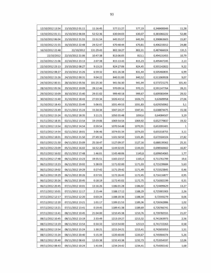
93

12/10/2012 13:54 13/10/2012 01:11 11:16:45 577:11:27 577,19 0,348400049 11,28

13/10/2012 01:11 15/10/2012 06:04 52:52:36 630:04:03 630,07 0,381066222 52,88

15/10/2012 06:04 15/10/2012 21:55 15:51:54 645:55:57 645,93 0,390863603 15,87

15/10/2012 21:55 16/10/2012 22:48 24:52:47 670:48:44 670,81 0,406233012 24,88

16/10/2012 22:48 22/10/2012 131:29:43 802:18:27 802,31 0,487466024 131,5

22/10/2012 22/10/2012 21:06 10:47:38 813:06:05 813,1 0,494131455 10,79

22/10/2012 21:06 22/10/2012 23:13 2:07:38 815:13:43 815,23 0,495447245 2,13

22/10/2012 23:13 23/10/2012 08:27 9:13:23 824:27:06 824,45 0,501142822 9,22

23/10/2012 08:27 23/10/2012 15:26 6:59:32 831:26:38 831,44 0,505460835 6,99

23/10/2012 15:26 24/10/2012 00:31 9:04:22 840:31:00 840,52 0,511069928 9,07

24/10/2012 00:31 28/10/2012 05:56 101:25:30 941:56:30 941,94 0,573721275 101,43

28/10/2012 05:56 29/10/2012 10:09 28:12:46 970:09:16 970,15 0,591147764 28,21

29/10/2012 10:09 30/10/2012 15:40 29:31:02 999:40:18 999,67 0,609383494 29,52

30/10/2012 15:40 31/10/2012 18:43 27:03:34 1026:43:52 1026,73 0,62609958 27,06

31/10/2012 18:43 31/10/2012 23:49 5:06:01 1031:49:53 1031,83 0,629250062 5,1

31/10/2012 23:49 01/11/2012 15:24 15:34:34 1047:24:27 1047,41 0,638874475 15,58

01/11/2012 15:24 01/11/2012 18:35 3:11:21 1050:35:48 1050,6 0,64084507 3,19

01/11/2012 18:35 02/11/2012 13:54 19:19:06 1069:54:54 1069,92 0,652779837 19,32

02/11/2012 13:54 02/11/2012 14:54 0:59:54 1070:54:48 1070,91 0,653391401 1

02/11/2012 14:54 02/11/2012 18:01 3:06:46 1074:01:34 1074,03 0,655318755 3,11

02/11/2012 18:01 03/11/2012 21:50 27:49:16 1101:50:50 1101,85 0,672504324 27,82

03/11/2012 21:50 04/11/2012 23:09 25:18:47 1127:09:37 1127,16 0,688139362 25,31

04/11/2012 23:09 05/11/2012 16:02 16:52:28 1144:02:05 1144,03 0,698560662 16,87

05/11/2012 16:02 05/11/2012 17:48 1:46:01 1145:48:06 1145,8 0,699654065 1,77

05/11/2012 17:48 06/11/2012 13:23 19:35:51 1165:23:57 1165,4 0,711761799 19,6

06/11/2012 13:23 06/11/2012 19:02 5:38:03 1171:02:00 1171,03 0,715239684 5,63

06/11/2012 19:02 06/11/2012 19:29 0:27:42 1171:29:42 1171,49 0,715523845 0,46

06/11/2012 19:29 06/11/2012 20:26 0:57:01 1172:26:43 1172,45 0,716116877 0,95

06/11/2012 20:26 06/11/2012 20:45 0:18:19 1172:45:02 1172,75 0,716302199 0,31

06/11/2012 20:45 07/11/2012 10:01 13:16:26 1186:01:28 1186,02 0,724499629 13,27

07/11/2012 10:01 07/11/2012 12:17 2:15:44 1188:17:12 1188,29 0,725901903 2,26

07/11/2012 12:17 07/11/2012 12:20 0:03:24 1188:20:36 1188,34 0,72593279 0,06

07/11/2012 12:20 07/11/2012 13:21 1:01:17 1189:21:53 1189,36 0,726562886 1,02

07/11/2012 13:21 07/11/2012 13:41 0:19:45 1189:41:38 1189,69 0,726766741 0,33

07/11/2012 13:41 08/11/2012 10:45 21:04:00 1210:45:38 1210,76 0,739782555 21,07

08/11/2012 10:45 08/11/2012 13:19 2:33:49 1213:19:27 1213,32 0,741363973 2,56

08/11/2012 13:19 08/11/2012 13:54 0:34:33 1213:54:00 1213,9 0,741722263 0,58

08/11/2012 13:54 08/11/2012 15:24 1:30:21 1215:24:21 1215,41 0,742655053 1,51

08/11/2012 15:24 08/11/2012 20:40 5:15:39 1220:40:00 1220,67 0,745904374 5,26

08/11/2012 20:40 09/11/2012 08:43 12:03:38 1232:43:38 1232,73 0,753354337 12,06

09/11/2012 08:43 09/11/2012 10:24 1:41:04 1234:24:42 1234,41 0,754392142 1,68

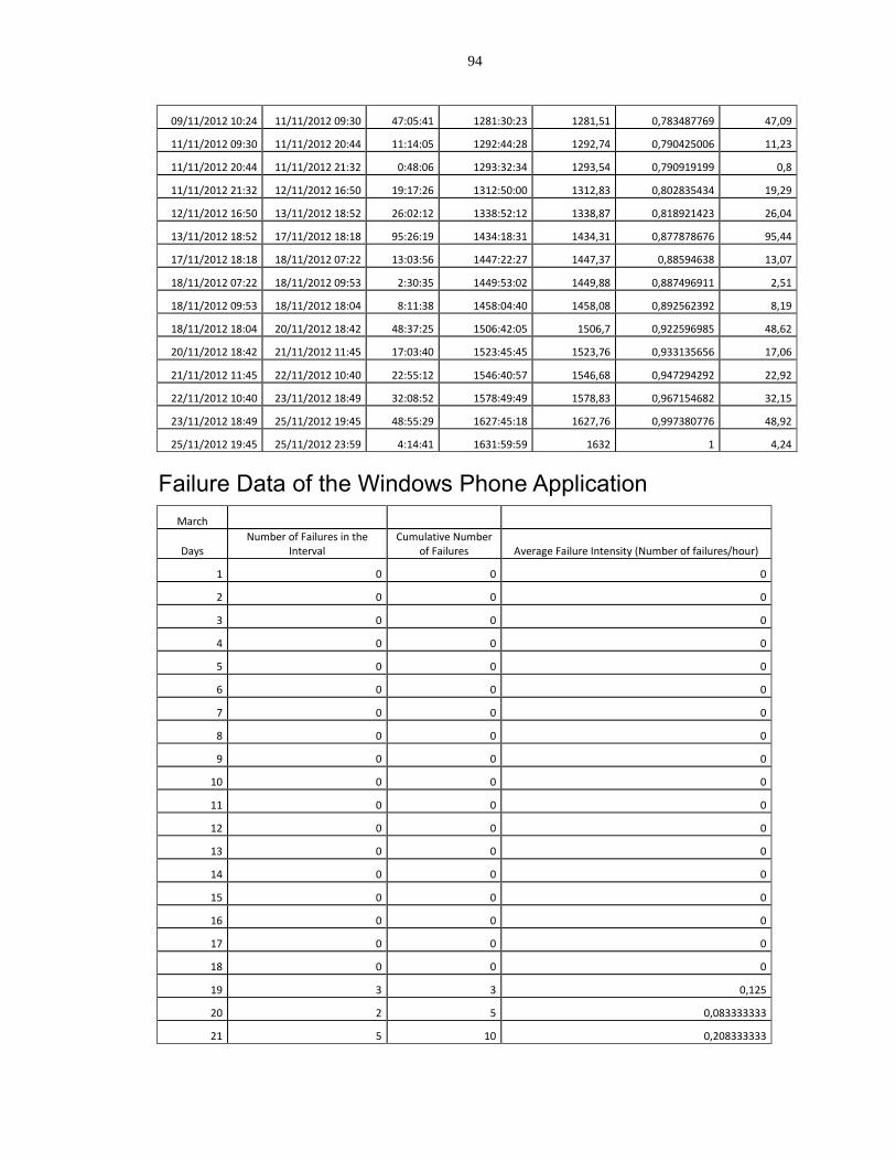
94

09/11/2012 10:24 11/11/2012 09:30 47:05:41 1281:30:23 1281,51 0,783487769 47,09

11/11/2012 09:30 11/11/2012 20:44 11:14:05 1292:44:28 1292,74 0,790425006 11,23

11/11/2012 20:44 11/11/2012 21:32 0:48:06 1293:32:34 1293,54 0,790919199 0,8

11/11/2012 21:32 12/11/2012 16:50 19:17:26 1312:50:00 1312,83 0,802835434 19,29

12/11/2012 16:50 13/11/2012 18:52 26:02:12 1338:52:12 1338,87 0,818921423 26,04

13/11/2012 18:52 17/11/2012 18:18 95:26:19 1434:18:31 1434,31 0,877878676 95,44

17/11/2012 18:18 18/11/2012 07:22 13:03:56 1447:22:27 1447,37 0,88594638 13,07

18/11/2012 07:22 18/11/2012 09:53 2:30:35 1449:53:02 1449,88 0,887496911 2,51

18/11/2012 09:53 18/11/2012 18:04 8:11:38 1458:04:40 1458,08 0,892562392 8,19

18/11/2012 18:04 20/11/2012 18:42 48:37:25 1506:42:05 1506,7 0,922596985 48,62

20/11/2012 18:42 21/11/2012 11:45 17:03:40 1523:45:45 1523,76 0,933135656 17,06

21/11/2012 11:45 22/11/2012 10:40 22:55:12 1546:40:57 1546,68 0,947294292 22,92

22/11/2012 10:40 23/11/2012 18:49 32:08:52 1578:49:49 1578,83 0,967154682 32,15

23/11/2012 18:49 25/11/2012 19:45 48:55:29 1627:45:18 1627,76 0,997380776 48,92

25/11/2012 19:45 25/11/2012 23:59 4:14:41 1631:59:59 1632 1 4,24

Failure Data of the Windows Phone Application

March

Days Number of Failures in the

Interval Cumulative Number

of Failures Average Failure Intensity (Number of failures/hour)

1 0 0 0

2 0 0 0

3 0 0 0

4 0 0 0

5 0 0 0

6 0 0 0

7 0 0 0

8 0 0 0

9 0 0 0

10 0 0 0

11 0 0 0

12 0 0 0

13 0 0 0

14 0 0 0

15 0 0 0

16 0 0 0

17 0 0 0

18 0 0 0

19 3 3 0,125

20 2 5 0,083333333

21 5 10 0,208333333

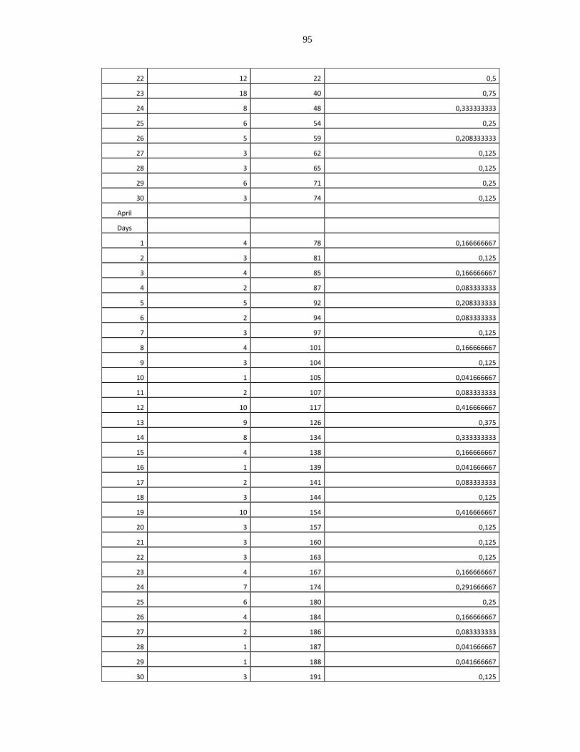
95

22 12 22 0,5

23 18 40 0,75

24 8 48 0,333333333

25 6 54 0,25

26 5 59 0,208333333

27 3 62 0,125

28 3 65 0,125

29 6 71 0,25

30 3 74 0,125

April

Days

1 4 78 0,166666667

2 3 81 0,125

3 4 85 0,166666667

4 2 87 0,083333333

5 5 92 0,208333333

6 2 94 0,083333333

7 3 97 0,125

8 4 101 0,166666667

9 3 104 0,125

10 1 105 0,041666667

11 2 107 0,083333333

12 10 117 0,416666667

13 9 126 0,375

14 8 134 0,333333333

15 4 138 0,166666667

16 1 139 0,041666667

17 2 141 0,083333333

18 3 144 0,125

19 10 154 0,416666667

20 3 157 0,125

21 3 160 0,125

22 3 163 0,125

23 4 167 0,166666667

24 7 174 0,291666667

25 6 180 0,25

26 4 184 0,166666667

27 2 186 0,083333333

28 1 187 0,041666667

29 1 188 0,041666667

30 3 191 0,125

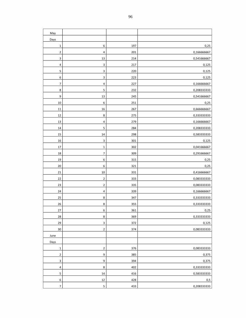
96

May

Days

1 6 197 0,25

2 4 201 0,166666667

3 13 214 0,541666667

4 3 217 0,125

5 3 220 0,125

6 3 223 0,125

7 4 227 0,166666667

8 5 232 0,208333333

9 13 245 0,541666667

10 6 251 0,25

11 16 267 0,666666667

12 8 275 0,333333333

13 4 279 0,166666667

14 5 284 0,208333333

15 14 298 0,583333333

16 3 301 0,125

17 1 302 0,041666667

18 7 309 0,291666667

19 6 315 0,25

20 6 321 0,25

21 10 331 0,416666667

22 2 333 0,083333333

23 2 335 0,083333333

24 4 339 0,166666667

25 8 347 0,333333333

26 8 355 0,333333333

27 6 361 0,25

28 8 369 0,333333333

29 3 372 0,125

30 2 374 0,083333333

June

Days

1 2 376 0,083333333

2 9 385 0,375

3 9 394 0,375

4 8 402 0,333333333

5 14 416 0,583333333

6 12 428 0,5

7 5 433 0,208333333

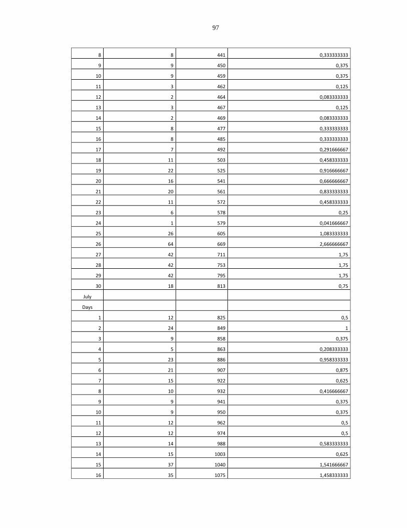
97

8 8 441 0,333333333

9 9 450 0,375

10 9 459 0,375

11 3 462 0,125

12 2 464 0,083333333

13 3 467 0,125

14 2 469 0,083333333

15 8 477 0,333333333

16 8 485 0,333333333

17 7 492 0,291666667

18 11 503 0,458333333

19 22 525 0,916666667

20 16 541 0,666666667

21 20 561 0,833333333

22 11 572 0,458333333

23 6 578 0,25

24 1 579 0,041666667

25 26 605 1,083333333

26 64 669 2,666666667

27 42 711 1,75

28 42 753 1,75

29 42 795 1,75

30 18 813 0,75

July

Days

1 12 825 0,5

2 24 849 1

3 9 858 0,375

4 5 863 0,208333333

5 23 886 0,958333333

6 21 907 0,875

7 15 922 0,625

8 10 932 0,416666667

9 9 941 0,375

10 9 950 0,375

11 12 962 0,5

12 12 974 0,5

13 14 988 0,583333333

14 15 1003 0,625

15 37 1040 1,541666667

16 35 1075 1,458333333

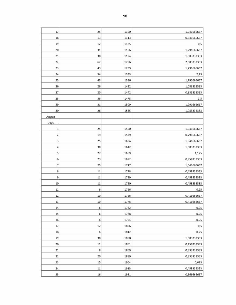
98

17 25 1100 1,041666667

18 13 1113 0,541666667

19 12 1125 0,5

20 31 1156 1,291666667

21 38 1194 1,583333333

22 62 1256 2,583333333

23 43 1299 1,791666667

24 54 1353 2,25

25 43 1396 1,791666667

26 26 1422 1,083333333

27 20 1442 0,833333333

28 36 1478 1,5

29 31 1509 1,291666667

30 26 1535 1,083333333

August

Days

1 25 1560 1,041666667

2 19 1579 0,791666667

3 25 1604 1,041666667

4 38 1642 1,583333333

5 27 1669 1,125

6 23 1692 0,958333333

7 25 1717 1,041666667

8 11 1728 0,458333333

9 11 1739 0,458333333

10 11 1750 0,458333333

11 6 1756 0,25

12 10 1766 0,416666667

13 10 1776 0,416666667

14 6 1782 0,25

15 6 1788 0,25

16 6 1794 0,25

17 12 1806 0,5

18 6 1812 0,25

19 38 1850 1,583333333

20 11 1861 0,458333333

21 8 1869 0,333333333

22 20 1889 0,833333333

23 15 1904 0,625

24 11 1915 0,458333333

25 16 1931 0,666666667

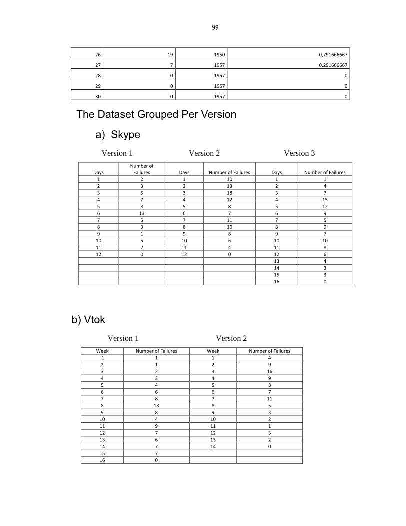
99

26 19 1950 0,791666667

27 7 1957 0,291666667

28 0 1957 0

29 0 1957 0

30 0 1957 0

The Dataset Grouped Per Version

a) Skype

Version 1 Version 2 Version 3

Days Number of

Failures Days Number of Failures Days Number of Failures

1 2 1 10 1 1

2 3 2 13 2 4

3 5 3 18 3 7

4 7 4 12 4 15

5 8 5 8 5 12

6 13 6 7 6 9

7 5 7 11 7 5

8 3 8 10 8 9

9 1 9 8 9 7

10 5 10 6 10 10

11 2 11 4 11 8

12 0 12 0 12 6

13 4

14 3

15 3

16 0

b) Vtok

Version 1 Version 2

Week Number of Failures Week Number of Failures

1 1 1 4

2 1 2 9

3 2 3 16

4 3 4 9

5 4 5 8

6 6 6 7

7 8 7 11

8 13 8 5

9 8 9 3

10 4 10 2

11 9 11 1

12 7 12 3

13 6 13 2

14 7 14 0

15 7

16 0

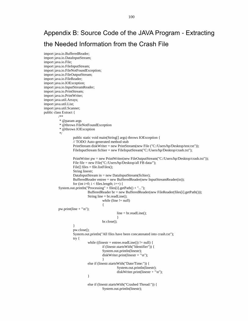
100

Appendix B: Source Code of the JAVA Program - Extracting

the Needed Information from the Crash File

import java.io.BufferedReader;

import java.io.DataInputStream;

import java.io.File;

import java.io.FileInputStream;

import java.io.FileNotFoundException;

import java.io.FileOutputStream;

import java.io.FileReader;

import java.io.IOException;

import java.io.InputStreamReader;

import java.io.PrintStream;

import java.io.PrintWriter;

import java.util.Arrays;

import java.util.List;

import java.util.Scanner;

public class Extract {

/**

* @param args

* @throws FileNotFoundException

* @throws IOException

*/

public static void main(String[] args) throws IOException {

// TODO Auto-generated method stub

PrintStream diskWriter = new PrintStream(new File ("C:/Users/hp/Desktop/test.txt"));

FileInputStream fichier = new FileInputStream("C:/Users/hp/Desktop/crash.txt");

PrintWriter pw = new PrintWriter(new FileOutputStream("C:/Users/hp/Desktop/crash.txt"));

File file = new File("C:/Users/hp/Desktop/all FB data/");

File[] files = file.listFiles();

String linestr;

DataInputStream in = new DataInputStream(fichier);

BufferedReader entree = new BufferedReader(new InputStreamReader(in));

for (int i=0; i < files.length; i++) {

System.out.println("Processing" + files[i].getPath() + "...");

BufferedReader br = new BufferedReader(new FileReader(files[i].getPath()));

String line = br.readLine();

while (line != null)

{

pw.print(line + "\n");

line = br.readLine();

}

br.close();

}

pw.close();

System.out.println("All files have been concatenated into crash.txt");

try {

while ((linestr = entree.readLine()) != null) {

if (linestr.startsWith("Identifier")) {

System.out.println(linestr);

diskWriter.print(linestr + "\n");

}

else if (linestr.startsWith("Date/Time:")) {

System.out.println(linestr);

diskWriter.print(linestr + "\n");

}

else if (linestr.startsWith("Crashed Thread:")) {

System.out.println(linestr);

101

diskWriter.print(linestr + "\n");

}

else if (linestr.startsWith("Highlighted Thread:")) {

System.out.println(linestr);

diskWriter.print(linestr + "\n");

}

else if (linestr.startsWith("OS Version:")) {

System.out.println(linestr);

diskWriter.print(linestr + "\n");

}

}

}

catch (IOException e) {

// TODO Auto-generated catch block

e.printStackTrace();

}

try {

in.close();

} catch (IOException e) {

// TODO Auto-generated catch block

e.printStackTrace();

}

entree.close();

}

}

102

Curriculum Vitae

Name: Sonia Meskini Post-secondary Faculty of Science of Tunisia (FST) Education and Manar 1, Tunis, Tunisia Degrees: 2006-2008 Math-Physics Preparatory school

The School of Engineers of Tunisia (ENIT) Manar 1, Tunis, Tunisia 2008-2011 Engineering Diploma in Computer Science

The University of Western Ontario London, Ontario, Canada 2011-2013 MESc in Software Engineering

Related Work Teaching Assistant Experience The University of Western Ontario

2011-2013

Publications:

S. Meskini, A. B. Nassif, and L. F. Capretz, “Reliability Models Applied to Mobile

Applications,” Proceedings of the 7th IEEE International Conference on Software

Security and Reliability Companion, Washington, D.C., IEEE Press, pp. 155-162, June

2013.

S. Meskini, L. F. Capretz, and A. B. Nassif, “Can We Rely on Smartphone

Applications?,” IEEE Computer, IEEE Press, submitted, July 2013.

S. Meskini, L. F. Capretz, and A. B. Nassif, “Reliability Prediction of Smartphone

Applications Through Their Failure Data Analysis,” 19th IEEE Pacific Rim International

Symposium on Dependable Computing, Vancouver, B.C., accepted, December 2013.