Optimal Taxation with Rent-Seeking∗

Casey RothschildWellesley College

Florian ScheuerStanford University

December 2015

Abstract

We develop a framework for optimal taxation when agents can earn their incomeboth in traditional activities, where private and social products coincide, and in rent-seeking activities, where private returns exceed social returns either because they in-volve the capture of pre-existing rents or because they reduce the returns to tradi-tional work. We characterize Pareto optimal income taxes that do not condition onhow much of an individual’s income is earned in each of the two activities. Theseoptimal taxes feature an externality-corrective term, the magnitude of which dependsboth on the Pigouvian correction that would obtain if rent-seeking incomes could beperfectly targeted and on the relative impact of rent-seeking externalities on the pri-vate returns to traditional and to rent-seeking activities. If rent-seeking externalitiesprimarily affect other rent-seekers, for example, the optimal correction lies strictly be-low the Pigouvian correction. A calibrated model indicates that the gap between thePigouvian and optimal correction can be quantitatively important. Our results thuspoint to a hefty informational requirement for correcting rent-seeking externalitiesthrough the income tax code.

∗Email addresses: crothsch@wellesley.edu, scheuer@stanford.edu. We are especially grateful to IvánWerning and two anonymous referees for numerous valuable suggestions. We also thank Daron Acemoglu,Alan Auerbach, Marco Bassetto, Michael Boskin, Paco Buera, V. V. Chari, Peter Diamond, Emmanuel Farhi,Mikhail Golosov, Martin Hellwig, Caroline Hoxby, Patrick Kehoe, Phillip Levine, Guido Menzio, Chris Phe-lan, Thomas Piketty, James Poterba, Emmanuel Saez, Daniel Sichel, Matthew Weinzierl, David Wildasin andseminar participants at Alberta, Berkeley, MPI Bonn, Cologne, Copenhagen, Cornell, Frankfurt, Guelph, theFederal Reserve Bank of Minneapolis, Harvard, Konstanz, Mannheim, Munich, MIT, Stanford, StockholmSchool of Economics, UMass-Amherst, Uppsala, Wellesley, Wharton, ETH Zurich, the SED Annual Meet-ing, NBER Summer Institute and Public Economics Program Meeting, Minnesota Workshop in Macroeco-nomic Theory, NTA Annual Conference on Taxation, the ASSA Meetings and the Young Macroeconomists’Jamboree (Duke) for helpful comments. Scheuer thanks Harvard University and UC Berkeley and Roth-schild thanks the Radcliffe Institute for Advanced Study at Harvard University for hospitality and funding.All errors are our own.

1 Introduction

The financial crisis exposed prominent examples of highly compensated individuals whoseapparent contributions to social output proved illusory. The view that some top incomesreflect rent-seeking—i.e., the pursuit of personal enrichment by extracting a slice of theexisting economic pie rather than by increasing the size of that pie—has inspired callsfor a more steeply progressive tax code (Piketty et al., 2014), and, motivated by similarconcerns about rent-seeking in finance, various countries have proposed higher taxes onfinancial-sector bonus payments (Besley and Ghatak, 2013).

The argument behind such proposals is intuitively appealing. If part of the economicactivity at high incomes is socially unproductive rent-seeking or “skimming,” then itwould seem natural for a well-designed income tax to impose high marginal rates at highincomes.1 This would discourage such behavior while simultaneously raising revenuethat could be used, for instance, to reduce taxes and encourage more productive effort atlower incomes. Moreover, if some sectors or professions are more prone to rent-seekingthan others (Lockwood et al., 2015), sector-specific corrective taxes would be useful.

In this paper, we study the optimal design of such policies under the assumption ofimperfect targeting. For example, lawyers produce many socially efficient services, uphold-ing property rights and providing incentives to abide by useful rules. On the other hand,they may also engage in rent-seeking activities, some of which resemble zero-sum games.The friction that we account for here is that it can be very hard to tell which is which: theonly way to find out can be a costly trial, a highly imperfect process. A similar point canbe made of finance and many other sectors. Hence, even sector- or profession-specifictaxes are necessarily imperfectly targeted, as they apply to multiple different activitieswithin such sectors that all come together in the same market and cannot be easily dis-entangled in any given transaction. At the extreme, an individual may engage both inproductive and rent-seeking activities simultaneously, but only total income is observ-able when computing tax liabilities.

Towards cleanly identifying the key effects of rent-seeking on optimal income taxes,we begin with a simple representative-agent Ramsey model which isolates the correctiverole for taxation—as there is no scope for redistribution. The identical individuals in thismodel can pursue two types of activities: traditional, productive work, where privateand social returns to effort coincide, and rent-seeking, where private returns exceed thesocial returns to effort. Suppose, for instance, that rent-seeking effort involves claimingcredit for productive work done by others. Then rent-seeking imposes across-activity

1See Bertrand and Mullainathan (2001) for evidence of such rents.

1

externalities (i.e., reduces the productivity of traditional effort) as well as within-activityexternalities (due to crowding effects in claiming credit). Both externalities drive a wedgebetween the private returns to effort and its true productivity at the aggregate level.

A natural guess for the optimal tax rate would be the weighted Pigouvian tax rate,i.e., the proportion of income earned through rent-seeking in the economy multiplied bythe wedge between the private and social returns to rent-seeking effort—the wedge thatwould be the optimal tax on rent-seeking if it could be separately identified. Our firstmain result, however, is that the optimal income tax systematically diverges from thisbenchmark (Proposition 1).

To see why the initial guess is generally incorrect, consider the effects of a small taxincrease. It discourages effort and thus directly reduces rent-seeking. But it also hasindirect effects since a reduction in rent-seeking effort raises the returns to both typesof effort. If the within-activity externalities are large relative to the across-activity ones,the returns to rent-seeking rise by more than the returns to productive effort. The taxchange thus encourages a perverse shift of effort into rent-seeking. This indirect effectpartially offsets the direct corrective benefits of the higher tax, and the optimal correctionlies strictly below the Pigouvian benchmark. When, on the other hand, the across-activityexternalities from rent-seeking dominate the within-activity ones, a reduction in rent-seeking effort lowers the relative returns to rent-seeking, the activity shift effect reversessign, and the optimal correction exceeds the Pigouvian tax rate.

Indeed, we provide a simple and intuitive formula for the optimal correction, whichreveals that the gap between the optimal and Pigouvain corrections depend on the prod-uct of two key parameters: the elasticity of the relative returns with respect to rent-seekingeffort, and individuals’ substitution elasticity between the two activities. The former de-termines the extent to which an additional unit of rent-seeking effort increases or de-creases the relative returns to rent-seeking, and the second determines the magnitude ofthe activity shift in response to a change in relative returns. Only in the knife-edge casewhere one of these elasticities is zero does the standard Pigouvian correction apply. Con-versely, we show that the divergence between the Pigouvian and the optimal correctionexplodes in this framework as the substitution elasticity grows (so individuals tend tospecialize in one of the two activities): The optimal tax can be zero even though rent-seeking accounts for a strictly positive share of income in the economy and even thoughit has strictly negative externalities.

We then extend our analysis to allow for heterogeneity, which is required both to ad-dress the question of the optimal progressivity of the income tax schedule, and also to seehow the corrective motives interact with the standard redistributive motives for taxation.

2

This extension assumes that individuals differ in their skills for both activities and consid-ers the design of a fully nonlinear income tax. We solve this multidimensional screeningmodel by building on the insights in Rothschild and Scheuer (2013). Specifically, we ob-serve that the realized wage distribution depends on the aggregate rent-seeking effort,so that the optimal tax problem can be treated as a fixed point problem for rent-seekingeffort nested within an almost-standard Mirrlees (1971) optimal tax problem. The bottomline is that the key intuition from the Ramsey model carries over, but the activity shifteffect gets complemented by several additional effects, which are due to heterogeneity.

In particular, our Proposition 2 provides an optimal marginal tax rate formula for eachincome level. This formula features a multiplicative correction to a standard optimal taxformula for economies without rent-seeking (such as Saez, 2001). This structure is consis-tent with the “principle of targeting” (Dixit, 1985) and, more specifically, the “additivityprinciple” discussed in the literature on corrective taxation in the presence of atmosphericexternalities, according to which taxes can be expressed as a sum of the optimal Pigou-vian taxes and the optimal taxes from a related problem without externalities.2 However,Proposition 3 shows that the correction term in the optimal tax formula again divergesfrom the Pigouvian benchmark in manner that depends in a transparent way on the signand magnitude of the relative return elasticity.

Interestingly, we find an even stronger divergence result (vis-à-vis the Ramsey model)in this heterogeneous agent model. The reason is that changes in marginal tax rates at anygiven income level affect aggregate returns and therefore induce activity shifts elsewherein the income distribution. As a result, the optimal correction diverges from the Pigouvianbenchmark even at points in the distribution where all income is from rent-seeking, andwhere the (marginal) income tax might appear to be a perfectly targeted instrument.

Finally, we complement these analytical results with a quantitative exploration of thisdivergence. We estimate a flexible bivariate Pareto-lognormal parametrization of the thetwo-dimensional skill distribution using data from the 2014 Current Population Survey(CPS) and borrow estimates for the externalities from rent-seeking, which we associatewith law and finance, from the literature. We then trace out the full set of possible relativereturn effects, consistent with the given Pigouvian correction, and simulate the optimalnonlinear income tax schedule for each of these scenarios. Our results suggest that thegeneral equilibrium effects we emphasize here can be of similar magnitude as the Pigou-vian taxes themselves, leading to considerable divergences.

In summary, our theoretical and quantitative results point to the hefty informationalrequirements for using the income tax code to correct rent-seeking externalities. Even

2See Sandmo (1975), Sadka (1978), Cremer et al. (1998), Kopczuk (2003).

3

if, for example, policymakers could perfectly pin down the overall magnitude of rent-seeking externalities, either in the economy overall or in a particular industry such as fi-nance (which is already challenging), our results suggest that there would still be a widerange of possibly optimal corrective taxes. To determine the appropriate corrective tax,policymakers would additionally need to know the relative impact of rent-seeking on var-ious activities. In the absence of clear evidence on this, our results can be interpreted asadvising caution in using the income tax as a tool to discourage rent-seeking.

Related Literature. Our main results are most closely related in spirit to Diamond (1973),although our motivation and framework are very different. Most importantly, Diamondanalyses the linear taxation of an externality-producing consumption good with hetero-geneous agents. We establish our results in a homogenous agent Ramsey setting and thenextend them to a Mirrleesian framework with non-linear income taxes, thereby incorpo-rating both corrective and redistributive motives for taxation. Moreover, as we discussin detail in the following section, our formula characterizing the divergence between theoptimal and Pigouvian corrections in the Ramsey model is related to some of Diamond’sformulas, but in contrast to them our formula shows that this divergence depends in anintuitive way on the product of two simple elasticities with natural empirical analogs,allowing us to get transparent results on its direction and magnitude.

A special case of our model obtains when rent-seeking income is earned through acrowdable search activity. Our analysis is therefore related to recent work by Golosov etal. (2013), who consider optimal taxation in labor markets with search frictions. However,they abstract from skill-driven wage heterogeneity in contrast to the general heterogene-ity we allow for. Moreover, they consider search for employment rather than search as anincome producing (but, through crowding, negative externality generating) activity (seealso Hungerbuhler et al., 2006).

Our analysis tracks the methods of the optimal income taxation literature, notablyRamsey (1927), Mirrlees (1971), Diamond (1998), Saez (2001) and Werning (2007). Ourpaper also contributes to recent efforts to study optimal taxation under multidimen-sional private heterogeneity—a literature which needs to tackle the challenges impliedby multidimensional screening problems, as standard techniques typically do not ap-ply (Rochet and Choné, 1998). This literature includes, for instance, Kleven et al. (2009),Scheuer (2013, 2014), Beaudry et al. (2009), Choné and Laroque (2010), and Lockwood andWeinzierl (2015). These papers have different information structures than ours, however:the second dimension of heterogeneity enters preferences additively in the first three; inBeaudry et al. (2009), types have two distinct labor productivities, but one activity is a

4

non-market activity, the returns from which are unobservable, whereas total income—but not its breakdown between the two activities—is observable in our model;3 and inChoné and Laroque (2010) and Lockwood and Weinzierl (2015), the second dimension isa taste for labor rather than a full second skill type as we employ here.

More closely related is Rothschild and Scheuer (2013), who use methods similar tothose developed here to characterize optimal taxation in a Roy (1951) model. That papershares the structure of two-dimensional heterogeneity in our Mirrlees extension, but (asall the other papers above) considers the special case where individuals always specializein one type of activity. It also rules out wages that deviate from the social marginal prod-uct of effort and the resulting corrective motives for taxation, issues we focus on here.4

Finally, our paper relates to the literature studying the equilibrium allocation of tal-ent across different sectors when there are rents to be captured in some of them. Mostof this literature (e.g. Baumol, 1990, Murphy et al., 1991, Acemoglu and Verdier, 1998,and Cahuc and Challe, 2012) does not consider optimal tax policy to correct these equilib-rium outcomes. But there are important recent exceptions. Philippon (2010) considers anendogenous growth model with financiers, workers and entrepreneurs and analyzes theeffect of linear, sector-specific taxes on growth. The recent studies by Piketty et al. (2014)and Lockwood et al. (2015) focus on the case where externalities reduce everyone else’sincome in a lump-sum fashion rather than the proportional reduction that we considerhere. This rules out the relative return effects from effort that we emphasize, which arisewhen the externalities can affect different activities to varying degrees. In this case, dueto the absence of general equilibrium effects, the simple weighted Pigouvian correctionis optimal, which we use as a benchmark to compare our results to, both analytically andquantitatively. Furthermore, Lockwood et al. abstract from redistributive motives andPiketty et al. restrict attention to top marginal tax rates.

This paper proceeds as follows. In Section 2, we begin with a representative agentRamsey model that illustrates the key force underlying our main divergence result. Sec-tion 3 then incorporates rich heterogeneity into our modeling framework and discussestax implementation issues. In Section 4, we analyze this model and provide our mainresults. Finally, Section 5 provides a quantification of these results for a calibrated versionof our model, and Section 6 concludes. Most proofs as well as details on the data and cal-ibration appear in a technical appendix. We also collect various examples and extensions

3Beaudry et al. also assume that, unlike here, effort in the market activity is observable.4Our Ramsey setting with two unobservable margins of effort also relates to the literature on multi-

tasking (Holmström and Milgrom, 1991 and Baker, 1992), although these papers do not consider externali-ties and corrective taxation. In Rothschild and Scheuer (2014), we extend our Mirrleesian analysis to N > 2activities with arbitrary positive and negative externalities.

5

in an online appendix.

2 A Simple Model Without Heterogeneity

We begin with a simple Ramsey representative agent model, which illustrates the keyforce underlying our results. We will later show the additional effects that emerge in arich Mirrlees model with more realistic heterogeneity.

2.1 Setup

Preferences. Consider an economy consisting of a unit mass of identical agents, indexedby i ∈ [0, 1]. Preferences over consumption c and effort in each of two distinct activities,eθ and eϕ, are given by U(c, eθ, eϕ) = u(c, m(eθ, eϕ)) ≡ u(c, l). We associate θ with atraditional activity and ϕ with rent-seeking, as explained below. We assume that u isstrictly quasiconcave, twice continuously differentiable, and has uc > 0 and ul < 0. Wealso impose the regularity conditions that consumption c and “leisure” −l are normalgoods and liml,c→0−ul/uc = 0. For concreteness, we consider here the CES-specificationfor the effort aggregator

m(eθ, eϕ) =

(e

1+σσ

θ + e1+σ

σϕ

) σ1+σ

with constant substitution elasticity σ > 0, but we show in Appendix A that our resultsgo through for more general specifications. For σ→ 0, individuals always choose eθ = eϕ,whereas for σ→ ∞, they always specialize in one of the two activities.

Technology. Agents earn incomes y in proportion to each of the two components oftheir effort via y = rθ(E)eθ + rϕ(E)eϕ, where the activity-specific returns rθ(E) = kθE−βθ

and rϕ(E) = kϕE−βϕ , with elasticities βθ, βϕ ∈ [0, 1), are decreasing in the aggregate rent-seeking effort E ≡

∫ 10 eϕ(i)di, and where kθ, kϕ > 0 are some constants.5 For later use,

denote the elasticity of the relative return rθ(E)/rϕ(E) with respect to E by ∆ ≡ βϕ − βθ.We also impose the regularity condition ∆σ > −1 + βθ, which we discuss further below.

Summing over individuals, aggregate income is therefore

Y(Eθ, E) = rθ(E)Eθ + rϕ(E)E, (1)

where Eθ ≡∫ 1

0 eθ(i)di. It is a sum of two components: the total earnings Yϕ ≡ rϕ(E)E

5Appendix A again shows that our results generalize to arbitrary non-increasing return functions, whoseelasticities with respect to E are not constant, but depend on E.

6

accruing to rent-seeking, and the total earnings Yθ ≡ rθ(E)Eθ accruing to the traditionalactivity. The private returns rθ to traditional effort thus coincide with the marginal socialreturns ∂Y/∂Eθ. On the other hand, unless βθ = βϕ = 0, the private returns rϕ to rent-seeking effort strictly exceed the marginal social returns ∂Y/∂E = rϕ − βθYθ/E− βϕrϕ.

Rent-seeking Externalities. The divergence between rϕ and ∂Y/∂E is why we interpretthe ϕ-activity as generalized rent-seeking. For example, when βθ = 0 and in the limitingcase βϕ → 1, there is a fixed “pie” of rents Yϕ = kϕ that individuals compete for byexerting effort eϕ. This pie is divided up across agents in proportion to their individualeffort eϕ. More generally, when βϕ < 1, Yϕ is increasing but concave in E, and a proportion1− βϕ of private rent-seeking earnings are attributable to increasing the size of the rent-seeking pie while the remaining portion βϕ is attributable to “skimming” from the portionof the pie that would otherwise have gone to other rent-seekers. Finally, when βθ >

0, rent-seeking effort additionally reduces the income Yθ in the traditional activity. Thedependence of the returns rθ(E) and rϕ(E) on aggregate rent-seeking effort reflects theserent-seeking externalities.

The magnitude of the rent-seeking externality is naturally measured by the Pigouviancorrection tPigou, which aligns the private returns rϕ to an additional unit of rent-seekingeffort eϕ with the social returns ∂Y/∂E to this unit. That is, tPigou is defined such that

(1− tPigou)rϕ =∂Y∂E

⇒ tPigou = βϕ +1− s

sβθ, (2)

where s ≡ Yϕ/Y is the aggregate income share of rent-seeking.

Tax Instruments. There is a benevolent social planner who is aware of the structure ofthe economy, but who is unable distinguish rent-seeking earnings from traditional earn-ings. If the planner could separately identify and tax the earnings from rent-seeking ef-forts, it would optimally impose the tax tPigou on rent-seeking earnings. Due to imperfecttargeting, however, its only policy tool is a tax on total income, with marginal rate t andlump sum transfer T. Faced with such a tax, each agent solves

maxeθ ,eϕ

u((1− t)(rθ(E)eθ + rϕ(E)eϕ) + T, m(eθ, eϕ)

), (3)

taking E and hence the returns to each activity as given. It will be useful to rewrite theagent’s problem equivalently as

7

maxl

{max

xu((1− t)

(rθ(E)

xlm(x, 1)

+ rϕ(E)l

m(x, 1)

)+ T, l

)}, (4)

where x ≡ eθ/eϕ and we used the fact that m is homogeneous of degree 1. One can thinkof this as decomposing the agent’s problem into an inner, extensive margin problem ofchoosing the effort ratio x across activities, and an outer, intensive margin problem ofchoosing overall effort l (again taking E as given). In particular, the inner maximizationis equivalent to choosing the effort ratio x to solve

wE ≡ maxx

rθ(E)x + rϕ(E)m(x, 1)

. (5)

Then the outer maximum in (3) is

maxl

u((1− t)wEl + T, l). (6)

Maximization problem (6) indicates that wE is interpretable as a wage. Except for the factthat this wage is endogenous to the aggregate rent-seeking effort in the economy, (6) is astandard problem for an agent facing a linear tax and choosing overall effort l.

2.2 Equilibrium

An equilibrium is a tuple (t, T, E, Eθ) with E = e∗ϕ(t, T, E) and Eθ = e∗θ (t, T, E), and

T = t(rθ(E)Eθ + rϕ(E)E

), (7)

so that the planner’s budget is balanced.

Equilibrium Set. The equilibrium condition E = e∗ϕ(t, T, E) can be thought of as a fixedpoint problem for E, given any tax system (t, T): Individuals take the returns and henceE as given when choosing their optimal rent-seeking effort eϕ. In equilibrium, this effortchoice has to be consistent with the E that was taken as given. As the following lemmademonstrates, this fixed point problem is well-behaved: it has a unique solution for any(t, T). Indeed, the lemma demonstrates that E, Eθ, 1 − t, l = m(Eθ, E), and Y are allco-monotonic within the set of equilibria.

Lemma 1. If (t, T, E, Eθ) and (t′, T′, E′, E′θ) are equilibria, then 1− t ≥ 1− t′ ⇔ E ≥ E′ ⇔Eθ ⇔ E′θ ⇔ m(Eθ, E) ≥ m(E′θ, E′)⇔ Y(Eθ, E) ≥ Y(E′θ, E′).

The proof of Lemma 1, which is in Appendix A, makes use of our regularity assump-tion ∆σ > −1 + βθ. Specifically, it shows that Eθ is proportional to E1+∆σ along the

8

equilibrium set, and hence traditional-sector output Yθ is proportional to E1+∆σ−βθ . If theregularity condition is violated, it is possible that Eθ → 0 and hence l = m(Eθ, E) → 0 asE→ 0. But Yθ → ∞ as E→ 0. In other words, it would be feasible to have arbitrarily largeoutput, and hence consumption, with arbitrarily small aggregated effort, because the re-turns to traditional work explode as aggregate rent-seeking effort vanishes. We focus onthe well-behaved case where this is excluded, and equilibria feature the co-monotonicityproperty established in Lemma 1.

2.3 Optimal Tax Policy

By Lemma 1, the set of equilibria can be parameterized by E, t, l, or Y. The social plan-ner’s problem is to select the equilibrium with the maximum u(Y, l). Per the followingproposition, this maximum exists and involves a tax rate t that satisfies a simple anduseful condition.

Proposition 1. The optimal tax exists, and satisfies

t =stPigou

1 + (1− s)σ∆≥ 0. (8)

Intuition. At first glance, one may think that the optimal tax should just equal the shareof rent-seeking income s in the economy, multiplied by the Pigouvian tax on rent-seekingtPigou, i.e. the numerator of (8). Indeed, this would be the optimal correction in partialequilibrium, for an individual agent holding fixed the behavior of all other agents.6

The proposition shows, however, that the optimal tax rate diverges from this naivePigouvian benchmark by an adjustment factor 1/(1 + (1− s)σ∆), which only disappearsin the knife-edge cases where the relative returns are fixed (so ∆ = 0) or individuals’ effortratio eθ/eϕ is fixed (so σ→ 0). The intuition is based on the general-equilibrium effects ofthe tax. The behavior of all other agents will not, in fact, stay fixed as an individual agentadjusts overall effort l in response to a tax change. An increase in one agent’s l is asso-ciated with an increase in rent-seeking effort eϕ, and hence aggregate E, and therefore acorresponding change in the relative returns rθ(E)/rϕ(E) (unless ∆ = 0). This relative re-turn change will lead all agents to adjust their effort ratio across the two activities (unlessσ → 0). The magnitude of this shift depends on the elasticity of substitution σ betweeneffort in the two sectors and the elasticity ∆ of relative returns.

6To see this, note that the private return to overall effort l is wE. Since eϕ = l/m(x, 1) and eθ = xl/m(x, 1),the social return to overall effort—holding the behavior of the other agents fixed—is ∂Y

∂Eθ

xm(x,1) +

∂Y∂Eϕ

1m(x,1) .

A simple calculation shows that 1− stPigou indeed fills the wedge between these two returns.

9

For example, suppose ∆ > 0, so an increase in aggregate rent-seeking effort has astronger negative effect on rent-seeking returns than on traditional returns. Then a taxincrease, by lowering individuals’ overall and hence rent-seeking effort, increases therelative returns to rent-seeking, and therefore induces a somewhat perverse shift of efforttowards rent-seeking. As a result, and per (8), the optimal tax is below the Pigouvianbenchmark. On the other hand, when ∆ < 0, the general equilibrium effects are flipped:the tax, by discouraging effort, induces a reduction in the relative returns and hence afurther flow out of rent-seeking. As a result, it is optimal to over-correct compared to thePigouvian tax.

Relation to Diamond (1973). The formula in (8) bears some resemblance to the resultsin Diamond (1973). In his model, heterogeneous households demand an externality-producing consumption good. He shows that the optimal linear tax, when it cannot bedifferentiated across households, can be expressed as the product of a Pigouvian correc-tion that captures the direct effect of the tax on the demand for the good, and an adjust-ment term that reflects indirect effects of the changes in consumption across householdsinduced by the direct effect. The adjustment depends in a complicated way on the co-variances between the degree to which different households contribute to the externalityper unit demanded, the sensitivities of their demands with respect to the externality, andtheir price sensitivities. In particular, it vanishes when households are identical.

In contrast, our general equilibrium effects result from effort choice along two inten-sive margins corresponding to two income-earning activities. The divergence we findarises because the tax cannot separately target them, even with identical households.Moreover, we are able to characterize in which direction and by how much the optimalcorrection should deviate from the Pigouvian tax rate as a function of the product of twosimple elasticities. As we demonstrate in the next sections, our results also generalizeto a Mirrleesian setting with non-linear income taxes, which allows us to show how thecorrective motives for taxation isolated here interact with redistributive motives.

2.4 An Example

Putting Numbers. The simplicity of the optimality condition in Proposition 1 facilitatesback-of-the-envelope calculations of the adjustment factor. In particular, substitute (2) in(8) to get

t =sβϕ + (1− s)βθ

1 + (1− s)∆σ, (9)

10

so the numerator is just the income-share weighted average of the return elasticities. Forexample, consider again the case with a fixed “pie” of rents but no cross-activity external-ities, so βθ = 0 and βϕ → 1. Then tPigou → 100%, ∆ = 1 and t = s/(1 + (1− s)σ). If theshare of rent-seeking income is, say, s = 10%, the naive Pigouvian benchmark for the taxis also 10%, but the optimal tax is t = 1/(10 + 9σ). Hence, with σ = 1, the optimal taxis t ≈ 5%, roughly only half as much as the Pigouvian correction; it is even lower withhigher substitution elasticities.

Of course, this reasoning ignores the fact that the share of rent-seeking income s atthe optimum is endogenous to the tax rate, so we cannot simply treat it as a parameter.However, it is straightforward to compute it for simple parametrizations of the utilityfunction, as any given t implies a unique s in equilibrium. For example, suppose thatutility is quasilinear in consumption and isoelastic with effort elasticity ε, so

u(c, l) = c− l1+ 1ε

1 + 1ε

.

Appendix A shows that, in equilibrium,

1− t = Ksε−σ

ε(1+σ)

(1− s

s

) 1+εβϕ∆ε(1+σ)

(10)

where K > 0 is some constant that depends on kθ and kϕ but is independent of σ. Equa-tions (9) and (10) thus jointly characterize the optimal t and s, for any given parameters.7

An Example with Extreme Divergence. More interestingly, we can use this example toformalize the observation that the activity shift effect, and hence the divergence betweenthe optimal tax and the Pigouvian benchmark, can become extreme as σ → ∞, i.e. whenindividuals always specialize in the sector that delivers the higher return. By our regu-larity condition, this exercise requires focusing on the case with ∆ > 0. The followingcorollary shows that the optimal tax approaches zero even though the Pigouvian bench-mark, as well as the share of rent-seeking income, remain strictly positive.

Corollary 1. Suppose ∆ > 0 and K < 1− βϕ. As σ→ ∞, the unique optimum involves

t→ 0, s→ Kε > 0, and tPigou → βϕ +1− Kε

Kεβθ > 0.

7Specifically, K ≡ (kϕ/kθ)(1+εβϕ)/(∆ε)k−1

ϕ . Hence, for any given t and s that satisfy (9), we can, conversely,always reverse-engineer the remaining free parameters, such as the constants kθ and kϕ, to make sure theequilibrium condition (10) is satisfied, validating the above computations, which treated s as a parameter.

11

As an illustrative example, consider again the case without cross-activity externalities,with βθ = 0 and βϕ = 1/2. Then tPigou = 50%. Moreover, suppose ε = 1 and wechoose the free parameter K to approach 1/2 from below. Then the corollary impliesthat the share of rent-seeking income s also approaches 50%, so the Pigouvian benchmarkstPigou → 25%. In other words, half the income in the economy comes from a rent-seekingactivity where private returns are twice as high as social marginal returns. Nonetheless,the optimal tax rate approaches 0, because of the shift effects emphasized here.

To see why, consider a single individual i and suppose she decreases her effort l bya small amount δl in response to a tax increase. Since this decreases her rent-seekingeffort, the direct effect will be to reduce the externalities she imposes on other agents. Butthere are also indirect effects: her decrease in rent-seeking effort will increase the relativereturns to rent-seeking, leading other individuals to reallocate their efforts towards rent-seeking. In fact, with σ → ∞, they re-allocate until the original relative returns, andhence E, are restored. (This is because, as σ→ ∞, the relative returns are effectively fixedat 1 in any interior equilibrium, to make individuals just indifferent between the twoactivities.) The net effect is that the total income earned in the economy goes down byexactly i’s reduced earnings wδl, and, since E is unchanged, the entire change in earningscomes from the traditional sector. To put it another way: the individual’s rent-seekingeffort is directly unproductive, but, by effectively discouraging other individuals frompursuing additional rent-seeking, it is indirectly productive. With σ → ∞ the indirectproductivity exactly equals the private returns to rent-seeking, and the optimal correction,taking general equilibrium effects into account, is exactly zero.

2.5 Introducing Heterogeneity

In this section, we have derived our main result, characterizing the divergence betweenthe optimal and Pigouvian correction, in a setting without heterogeneity. In the remainderof the paper, we will show how this result extends to a richer setting where individualsdiffer in their skills for both activities and the planner has access to a nonlinear income taxand maximizes some social welfare function.8 We will see that the intuition emphasizedso far will continue to play a prominent role, but will be complemented by the followingadditional insights:

1. Most obviously, there will be redistributive motives across endogenously heteroge-neous wages. We will show how they interact with the purely corrective motives

8Such a more general framework will also be more suitable for calibration, allowing for a less ad hocquantification of the optimal divergence (see Section 5).

12

considered so far.

2. The activity shift effect featured in the denominator of (8) will reappear (and will belabeled effect S below), but it will play a somewhat different role with heterogeneity.Changes in rent-seeking effort at any given wage level affect aggregate returns andwill therefore induce activity shifts elsewhere in the wage distribution. As a result,the shift effect S will be global in nature. This will imply an even stronger divergenceresult, where the optimal correction diverges from the Pigouvian benchmark evenat wage levels where the share of rent-seeking income is 1, and where the (marginal)income tax might appear to be a perfectly targeted instrument.9

3. Because the wage distribution is endogenous to aggregate rent-seeking effort, theoptimal tax policy will seek to manipulate it in order to relax incentive constraints(labeled effect I below). This Stiglitz (1982)-type emerges more generally in settingswith general equilibrium effects (e.g. Rothschild and Scheuer, 2013).

4. More interestingly, there will be heterogeneity not just across wages, but also withinwages. For example, there will be individuals who earn the same wage but througha different mix of effort across the two activities, and who will therefore be differen-tially affected by changes in relative returns induced by changes in taxes. This leadsto additional activity shifts (labeled effect C below) as well as redistributive effects(effect R) within a given wage.

We will provide conditions under which the additional effects I, C and R all reinforcethe fundamental shift effect S that we already illustrated in this section, so that the resultin Proposition 1 goes through qualitatively.

3 The General Model

3.1 Setup

Skill Heterogeneity. As before, individuals can pursue two activities: Traditional workand rent-seeking. Individuals are now endowed with a two-dimensional skill vector(θ, ϕ) ∈ Θ × Φ, Θ = [θ, θ], Φ = [ϕ, ϕ], where θ captures an individual’s skill for tradi-tional work, and ϕ captures her skill for rent-seeking. In the preceding section, all agents

9In the online appendix, we provide a simple, stark example with two types that illustrates this point.

13

had identical skills (normalized to θ = ϕ = 1). Now, we let skills be distributed withsome general, continuous cdf F : Θ×Φ→ [0, 1] and associated continuous pdf f (θ, ϕ).10

Technology. Let the activity-specific efforts of an individual of type (θ, ϕ) be denotedby eθ(θ, ϕ) and eϕ(θ, ϕ), respectively. As before, aggregate output is given by (1), wherewe now define

Eθ ≡∫

Θ×Φθeθ(θ, ϕ)dF(θ, ϕ) and E ≡

∫Θ×Φ

ϕeϕ(θ, ϕ)dF(θ, ϕ)

as the aggregate effective (i.e., skill-weighted) efforts in the traditional and rent-seeking ac-tivities, respectively. Correspondingly, individuals earn income in proportion to their ef-fective effort in each activity, so y(θ, ϕ) = rθ(E)θeθ(θ, ϕ) + rϕ(E)ϕeϕ(θ, ϕ). To capture thedistinction between rent-seeking and traditional work, we again assume that both returnsrθ(E) and rϕ(E) are decreasing in aggregate rent-seeking effort E, but are independent oftraditional effort Eθ. As a result, the private return to effective effort coincides with thesocial marginal product in the traditional activity, but exceeds it in the rent-seeking ac-tivity, as in the previous section. Let the elasticities of the returns with respect to E bedenoted by βθ(E) = −r′θ(E)E/rθ(E) and βϕ(E) = −r′ϕ(E)E/rϕ(E) and the elasticity ofthe relative return to traditional work rθ/rϕ by ∆(E) ≡ βϕ(E) − βθ(E). ∆(E) measuresthe relative importance of within- versus across-activity externalities.

It is worth pointing out that this specification of technology is very general. In particu-lar, it is implied by any model where (i) each unit of effective effort in a given activity hasthe same private return, (ii) effort in the Θ-activity imposes no externalities, and (iii) ef-fort in the Φ-activity imposes at least weakly negative externalities on both activities. Wealso emphasize that this technology does not require firms or employers. We can assumethat each worker is self-employed and reaps the return to his effort directly. However, thereturns to both traditional and rent-seeking effort are determined in general equilibrium,by the supply of effort of all other workers. Finally, note that property (i) implies that therent-seeking externality works through individual returns to effective effort. It thereforerules out the uniform absolute reduction in other individuals’ incomes due to rent-seeking(considered, for instance, in Piketty et al., 2014, and Lockwood et al., 2015), which is inde-pendent of effort. Indeed, the interesting relative return effects on activity choice that weexplore in the following arise precisely because we allow rent-seeking to have differentialeffects on the returns to different types of effort.11

10See Section 6 for a discussion of how our framework can be extended to capture further heterogeneityin the disutility from, or taste for, working in the two activities.

11In the online appendix, we discuss several examples and applications that can be captured by our

14

Preferences. We consider the same utility function as in Section 2, given by U(c, eθ, eϕ) =

u(c, m(eθ, eϕ)) ≡ u(c, l). In the appendix, we will show that all our results hold for a gen-eral effort aggregator m(eθ, eϕ) that is increasing in both arguments, continuously differ-entiable, quasiconvex and linear homogeneous.12 To simplify the exposition, in the maintext we will focus our discussion on the special case where individuals always specializein one activity. This always obtains when m(eθ, eϕ) is linear, and corresponds most natu-rally to the interpretation of activities as tied to sectors or occupations (which is also theapplication we will consider in our numerical illustration in Section 5). In this case, onecan think of individuals as making an extensive margin choice, picking one of the two sec-tors depending on relative returns, and an intensive margin choice, picking the amountof effort they want to provide in the chosen sector, as in the Roy model considered inRothschild and Scheuer (2013).

When m is strictly quasiconvex, individuals generally choose some interior effort mixx = eθ/eϕ. Still, as seen in the previous section, one can decompose the individual’s prob-lem into two very similar subproblems: a choice of the effort ratio x, which (due to thelinear homogeneity of m) is again pinned down by the relative returns to the two activi-ties, and an intensive margin choice of l. This can capture situations where an individual’sjob involves a mixture of both rent-seeking and traditional, productive activities.

In the Ramsey model from the previous section, we saw that as we approached thecase with linear m, and hence the substitution elasticity σ → ∞, we could obtain un-bounded shift effects and therefore extreme results for optimal taxes. With heterogeneity,however, this connection no longer holds, because a linear m at the individual level doesnot imply an infinite substitution elasticity at the aggregate level. Intuitively, we will seethat most individuals’ sectoral choices are not responsive at all to small changes in rel-ative returns (as their skills are such that they strictly prefer working in one of the twosectors). Only the small set of individuals who were close to indifferent between the twosectors before the change do respond, leading to a finite and well-behaved aggregate shifteffect even in a model with full specialization.

framework, including the contests and races with winner-takes-all compensation that are widespread infinance, law, and research.

12Note that, since u is left general, this allows for preferences u(c, m(eθ , eϕ)) where m is homothetic butnot linear homogeneous: then there exist transformations u and m of u and m such that u(c, m(eθ , eϕ)) =u(c, m(eθ , eϕ)) for all (c, eθ , eϕ) with linear homogeneous m. An example is u(c)− hθ(eθ)− hϕ(eϕ) with hθ(.)and hϕ(.) homogeneous of the same degree.

15

3.2 Implementation

A Direct Mechanism. We respectively denote the consumption, effort, utility and activ-ity assigned to an individual of type (θ, ϕ) by c(θ, ϕ), l(θ, ϕ), V(θ, ϕ) ≡ u(c(θ, ϕ), l(θ, ϕ))

and S(θ, ϕ) ∈ {Θ, Φ}. We also define an individual’s wage as the return to effort in theassigned activity, so that

wE(θ, ϕ) =

{rθ(E)θ if S(θ, ϕ) = Θrϕ(E)ϕ if S(θ, ϕ) = Φ

and we can write an individual’s income simply as y(θ, ϕ) = wE(θ, ϕ)l(θ, ϕ). As is stan-dard, we assume the single crossing property, i.e., that the marginal rate of substitutionbetween y and c, −ul(c, y/w)/(wuc(c, y/w)), is decreasing in w.

We now describe a direct mechanism where individuals announce their privatelyknown type (θ, ϕ) and then get allocated c(θ, ϕ), y(θ, ϕ), and S(θ, ϕ). We will then linkthis to the implementation through a nonlinear income tax schedule T(y) using the re-sults in Rothschild and Scheuer (2013). In line with the imperfect targeting consideredin the Section 2, we take only income and consumption as de facto contractible for thegovernment, but not an individual’s skill type, sector, wage and effort.13 The resultingincentive constraints that guarantee truth-telling of (θ, ϕ) in the direct mechanism are:

u(

c(θ, ϕ),y(θ, ϕ)

wE(θ, ϕ)

)≥ max

{u(

c(θ′, ϕ′),y(θ′, ϕ′)

rθ(E)θ

), u(

c(θ′, ϕ′),y(θ′, ϕ′)

rϕ(E)ϕ

)}∀(θ′, ϕ′)

(11)since type (θ, ϕ) can imitate any other type (θ′, ϕ′) by earning (θ′, ϕ′)’s income either inthe Θ- or the Φ-activity.

An Income Tax Implementation. The following lemma, due to Rothschild and Scheuer(2013), shows that any incentive compatible allocation can be implemented by offering anonlinear income tax T(y).

Lemma 2. Any incentive compatible allocation {c(θ, ϕ), y(θ, ϕ), S(θ, ϕ), E} is such that(i)

wE(θ, ϕ) = max{rθ(E)θ, rϕ(E)ϕ} and S(θ, ϕ) =

{Θ if rθ(E)θ > rϕ(E)ϕ

Φ if rθ(E)θ < rϕ(E)ϕ;

(ii) u(c(θ, ϕ), y(θ, ϕ)/w) = u(c(θ′, ϕ′), y(θ′, ϕ′)/w) for all (θ, ϕ), (θ′, ϕ′) such that wE(θ, ϕ) =

wE(θ′, ϕ′) = w;

13See Section 6 for a discussion of these assumptions.

16

(iii) it can be implemented by offering a nonlinear income tax schedule T(y) and letting agentschoose their preferred (c, y)-bundle from the resulting budget set B = {(c, y)|c ≤ y− T(y)}.

The first two properties say that individuals always specialize in the activity wheretheir return to effort is higher and that individuals with the same wage must obtain thesame utility. The third property establishes that the principle of taxation holds. The sec-ond property does not rule out that two individuals with the same wage (but who spe-cialize in different activities) choose different (c, y)-bundles. Nonetheless, as argued inRothschild and Scheuer (2013), we can restrict attention to allocations {c(w), y(w), E} thatpool all same-wage individuals at the same (c, y)-bundle. The reason is that such poolingcan always be done in an incentive compatible and resource feasible way, and such thatit does not affect E or, by property (ii), utilities.

In Appendix B, we show how these results generalize to the case where individualsdo not necessarily specialize in one of the two activities, but pursue both simultaneously.Instead of assigning an activity from the binary set {Θ, Φ}, an allocation then specifiesthe share of income qE ∈ [0, 1] that an individual earns in the traditional activity (andconversely 1− qE is earned through rent-seeking). Defining the wage analogously to (5) inSection 2, our analysis goes through and Lemma 2 applies. In particular, any individual’swage wE and income share qE are fully pinned down by aggregate rent-seeking effort Ebut are independent of the rest of the allocation. Because all individuals with the samewage have the same preferences over (c, y)-bundles given by u(c, y/w), the screeningproblem can again be reduced to offering allocations {c(w), y(w)} that only condition onwages, which in turn are endogenous to E.

4 Optimal Non-linear Income Taxation

In this section, we characterize the set of Pareto efficient nonlinear income tax schedules.This allows us to compare the optimal and Pigouvian corrections in this richer setting.

4.1 Pareto Optima

Wage Distributions. Lemma 2 showed that fixing E determines the wage wE(θ, ϕ) andactivity choice of each type (θ, ϕ). Together with the two-dimensional skill distributionF(θ, ϕ), it therefore determines a one-dimensional wage distribution with cdf

FE(w) = F(

wrθ(E)

,w

rϕ(E)

)

17

and sectoral densities

f θE(w) =

1rθ(E)

∫ w/rϕ(E)

ϕf(

wrθ(E)

, ϕ

)dϕ, f ϕ

E (w) =1

rϕ(E)

∫ w/rθ(E)

θf(

θ,w

rϕ(E)

)dθ

with corresponding cdfs FθE(w) and Fϕ

E (w) and with fE(w) = f θE(w) + f ϕ

E (w). Hence,f ϕE (w)/ fE(w) is the share of rent-seekers at wage level w. We denote the support of the

wage distribution for any E by [wE, wE], where wE = wE(θ, ϕ) and wE = wE(θ, ϕ).14

Pareto Weights. We use general cumulative Pareto weights Ψ(θ, ϕ) in (θ, ϕ)-space withthe corresponding density ψ(θ, ϕ) to obtain Pareto efficient allocations. The social plannermaximizes

∫Θ×Φ V(θ, ϕ)dΨ(θ, ϕ) subject to resource and self-selection constraints. Com-

pletely analogously to the wage distributions above, for any given E, we can derive Paretoweights over wages ΨE(w), as well as their density and decomposition across activitiesψE(w) = ψθ

E(w) + ψϕE(w), from Ψ(θ, ϕ). We are particularly interested in the regular

case in which the planner assigns greater weight to low-wage individuals, i.e., whereψE(w)/ fE(w) is non-increasing in w for any E.15

Elasticities. Any incentive compatible allocation {c(w), y(w), E} implies total effort andutility l(w) ≡ y(w)/w and V(w) ≡ u(c(w), l(w)). We denote the resulting uncompen-sated and compensated wage elasticities of total effort l by εu(w) and εc(w), respectively.

A Decomposition of the Pareto Problem. As in Rothschild and Scheuer (2013), we candecompose the problem of finding Pareto optimal allocations into two steps. The firststep involves finding the optimal level of aggregate rent-seeking effort E. We call thisthe “outer” problem. The second (which we call the “inner” problem) involves findingthe optimal resource-feasible and incentive-compatible allocation for a given level of E.This inner problem is an almost standard Mirrlees problem; the only difference is that theinduced level of aggregate effective rent-seeking effort has to be consistent with the levelof E that we are fixing for the inner problem. For some given Pareto weights Ψ(θ, ϕ) (andhence induced weights ΨE(w)), we therefore define the inner problem as follows (where

14We show in Appendix C how these definitions can be extended to the case of a general effort aggregatorm, with the interpretation that f θ

E(w) and f ϕE (w) are the average value of q (respectively 1− q) at wage level

w. Hence, more generally, f ϕE (w)/ fE(w) is the share of rent-seeking income at w.

15For example, consider the case of relative Pareto weights where Ψ(θ, ϕ) = Ψ(F(θ, ϕ)) for some increas-ing function Ψ : [0, 1]→ [0, 1]. Then these Pareto weights are regular whenever Ψ is weakly concave.

18

c(V, e) is the inverse function of u(c, l) with respect to c):

W(E) ≡ maxV(w),l(w)

∫ wE

wE

V(w)dΨE(w) (12)

subject toV′(w) + ul(c(V(w), l(w)), l(w))

l(w)

w= 0 ∀w ∈ [wE, wE] (13)

rϕ(E)E−∫ wE

wE

wl(w) f ϕE (w)dw = 0 (14)

∫ wE

wE

wl(w) fE(w)dw−∫ wE

wE

c(V(w), l(w)) fE(w)dw ≥ 0. (15)

We employ the standard Mirrleesian approach of optimizing directly over allocations,i.e., over effort l(w) and consumption or, equivalently, utility V(w) profiles. The socialplanner maximizes a weighted average of individual utilities V(w) subject to three con-straints. (15) is a standard resource constraint and (14) ensures that aggregate effectiveeffort in the rent-seeking activity indeed sums up to E (or, equivalently, rent-seeking in-comes sum to rϕ(E)E). Finally, the allocation V(w), l(w) needs to be incentive compatible,i.e.,

V(w) ≡ u(c(w), l(w)) = maxw′

u(

c(w′),l(w′)w′

w

). (16)

It is a well-known result that under single-crossing, the global incentive constraints (16)are equivalent to the local incentive constraints (13) and the monotonicity constraint thatincome y(w) must be non-decreasing in w.16 We follow the standard approach of drop-ping the monotonicity constraint, which can easily be checked ex post (as we do for thenumerical simulations in Section 5). If the solution to problem (12) to (15) does not satisfyit, optimal bunching would need to be considered. Accounting for bunching is conceptu-ally straightforward and does not substantively effect our analysis, so, for simplicity, weabstract from bunching henceforth.

Once a solution V(w), l(w) to the inner problem has been found, the resulting welfareis given by W(E). The outer problem is then simply maxE W(E). It is straightforward toshow that a solution to the inner problem exists for any E (see Rothschild and Scheuer,2014, for details) and that, at any E for which individuals work in both activities, W(E) iscontinuous, so that the outer problem has a solution over any compact set of Es.17

16See, for instance, Fudenberg and Tirole (1991), Theorems 7.2 and 7.3.17Compactness would be ensured, for instance, by a standard Inada condition ul(c, l) → −∞ as l ↑ l for

some l < ∞.

19

4.2 Marginal Tax Rate Formulas from the Inner Problem

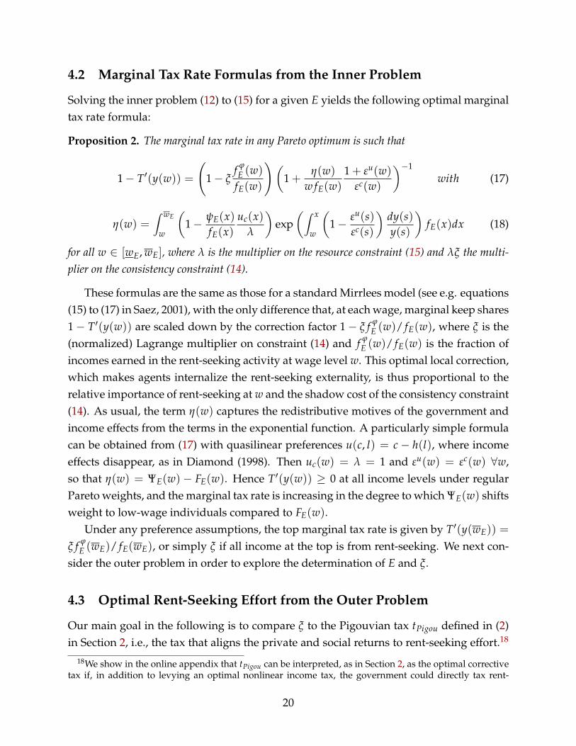
Solving the inner problem (12) to (15) for a given E yields the following optimal marginaltax rate formula:

Proposition 2. The marginal tax rate in any Pareto optimum is such that

1− T′(y(w)) =

(1− ξ

f ϕE (w)

fE(w)

)(1 +

η(w)

w fE(w)

1 + εu(w)

εc(w)

)−1

with (17)

η(w) =∫ wE

w

(1− ψE(x)

fE(x)uc(x)

λ

)exp

(∫ x

w

(1− εu(s)

εc(s)

)dy(s)y(s)

)fE(x)dx (18)

for all w ∈ [wE, wE], where λ is the multiplier on the resource constraint (15) and λξ the multi-plier on the consistency constraint (14).

These formulas are the same as those for a standard Mirrlees model (see e.g. equations(15) to (17) in Saez, 2001), with the only difference that, at each wage, marginal keep shares1− T′(y(w)) are scaled down by the correction factor 1− ξ f ϕ

E (w)/ fE(w), where ξ is the(normalized) Lagrange multiplier on constraint (14) and f ϕ

E (w)/ fE(w) is the fraction ofincomes earned in the rent-seeking activity at wage level w. This optimal local correction,which makes agents internalize the rent-seeking externality, is thus proportional to therelative importance of rent-seeking at w and the shadow cost of the consistency constraint(14). As usual, the term η(w) captures the redistributive motives of the government andincome effects from the terms in the exponential function. A particularly simple formulacan be obtained from (17) with quasilinear preferences u(c, l) = c− h(l), where incomeeffects disappear, as in Diamond (1998). Then uc(w) = λ = 1 and εu(w) = εc(w) ∀w,so that η(w) = ΨE(w)− FE(w). Hence T′(y(w)) ≥ 0 at all income levels under regularPareto weights, and the marginal tax rate is increasing in the degree to which ΨE(w) shiftsweight to low-wage individuals compared to FE(w).

Under any preference assumptions, the top marginal tax rate is given by T′(y(wE)) =

ξ f ϕE (wE)/ fE(wE), or simply ξ if all income at the top is from rent-seeking. We next con-

sider the outer problem in order to explore the determination of E and ξ.

4.3 Optimal Rent-Seeking Effort from the Outer Problem

Our main goal in the following is to compare ξ to the Pigouvian tax tPigou defined in (2)in Section 2, i.e., the tax that aligns the private and social returns to rent-seeking effort.18

18We show in the online appendix that tPigou can be interpreted, as in Section 2, as the optimal correctivetax if, in addition to levying an optimal nonlinear income tax, the government could directly tax rent-

20

The key question will be how ξ—interpretable the optimal externality correction in ourmodel with imperfect targeting—differs from the targeted instrument benchmark tPigou.

Welfare Effects of Changing E. To be able to answer this question, Lemma 3 providesan important auxiliary result, namely a decomposition of the welfare effect of marginalchanges in E that will be useful in the following.

Lemma 3. The welfare effect of a marginal change in aggregate rent-seeking effort E is

W ′(E) = λrϕ(E)(ξ − tPigou

)+

∆(E)E

[I + R + ξλ (C + S)] , (19)

whereI ≡ λ

∫ wE

wE

η(w)wV′(w)

uc(w)

ddw

(f ϕE (w)

fE(w)

)dw, (20)

R ≡∫ wE

wE

V′(w)wf θE(w) f ϕ

E (w)

fE(w)

(ψθ

E(w)

f θE(w)

−ψ

ϕE(w)

f ϕE (w)

)dw, (21)

C ≡∫ wE

wE

w2l′(w)f θE(w) f ϕ

E (w)

fE(w)dw (22)

andS ≡

∫ wE

wE

w2l(w) f(

wrθ(E)

,w

rϕ(E)

)dw ≥ 0. (23)

Direct Effects. The first term λξrϕ(E) in (19) is simply the direct effect of a change inE on the consistency constraint (14), holding effort and sector constant for each individ-ual. Similarly, the second term −λtPigourϕ(E) captures the effect of changing sectoralreturns on the resource constraint (15), holding effort, sector and consumption fixed forall types.19 In fact, when ∆(E) = 0, E has no effect on relative returns rθ(E)/rϕ(E). Sochanging E while holding the effort and activity choice for each type (θ, ϕ) fixed is com-patible with the incentive constraints (11). By an envelope argument, then, W ′(E) =

λ(ξ − tPigou

)rϕ(E), consistent with (19).

When ∆(E) 6= 0, the change in relative returns drives a wedge between ξ and tPigou

since holding allocations fixed is no longer incentive compatible, and there are additionalwelfare effects from a change in E captured by the four effects in (20) to (23), which areparallel to those in Rothschild and Scheuer (2013). In discussing them, we focus on the

seeking income (see Proposition 1 there).19To see this, differentiate with respect to E′ the total income in the economy rθ(E′)Eθ + rϕ(E′)E to get

(evaluated at E′ = E) r′θ(E)Eθ + r′ϕ(E)E = ∂Y(Eθ , E)/∂E− rϕ(E) = −rϕ(E)tPigou.

21

case ∆(E) > 0, so that an increase in E increases the relative return to traditional workrθ/rϕ. The opposite case is analogous with reversed signs.

Activity Shift Effect. A change in E causes an activity or sectoral shift, analogous to theone found in the Ramsey model in Section 2. An increase in E (and thus rθ/rϕ) leadssome previously indifferent individuals to switch from rent-seeking to traditional work;S measures the effort shifted as a result.20 In the representative agent Ramsey model ofSection 2, the activity shift was the sole driver of the divergence between the optimal andthe Pigouvian correction.

Novel Effects due to Heterogeneity. The additional effects C, R and I arise from the richheterogeneity in the Mirreleesian framework. Specifically, they arise because a change inE has differential wage effects on distinct individuals.

The term I is a generalized Stiglitz (1982) effect, which arises because the magnitudeof the wage effects varies across the wage distribution. If ∆ > 0 and the share of incomeearned through rent-seeking is locally increasing in w (i.e., d( f ϕ

E (w)/ fE(w))/dw > 0),then an increase in E leads to a local compression of the wage distribution, as returnsin the high-wage activity fall relative to the low-wage activity. This yields a welfare-improving easing of the local incentive constraints (13) if they are binding downwards(η(w) ≥ 0). I therefore vanishes if there are no redistributive motives (e.g. with quasilin-ear preferences and Ψ(F) = F ∀F), so that η(w) = 0 for all w.

Moreover, a change in E has different effects on the wages of distinct individuals whooriginally earned the same wage w. In particular, the wage of a traditional worker at wfalls by r′θ(E)w/rθ(E) = βθ(E)w/E whereas the wage of a rent-seeker falls by βϕ(E)w/E.Hence, when ∆(E) > 0, the rent-seekers at w see their wages fall by more than the averagefor the wage w-workers, and the traditional workers see their wages fall by less. Theterm C arises because, by changing their wages differentially in the face of a fixed effortschedule l(w), an increase in E in effect re-allocates effort across the rent-seekers andtraditional workers who are originally pooled. In particular, for an increasing (in w) effortschedule, a rise in E results in a re-allocation of effort from rent-seekers (who effectivelymove down along the schedule) to traditional workers (who move up) at any given w.

20We show in Appendix C.3 how S can be generalized to allow for general m, in which case it will alsoincorporate continuous changes in the effort ratio eθ/eϕ in response to the relative return change, as inSection 2.

22

Hence, C reinforces S if l′(w) ≥ 0.21

The term R arises from the analogous reallocation of utility V(w) from rent-seekersto traditional workers at the same initial wage, which is why it shows up in parallel tothe redistributive Stiglitz-term I. It disappears with relative welfare weights Ψ(θ, ϕ) =

Ψ(F(θ, ϕ)), since then ψθE(w)/ f θ

E(w) = ψϕE(w)/ f ϕ

E (w) for all w, E. Otherwise, it is wel-fare improving when the planner puts more weight on traditional workers at each wage(ψθ

E(w)/ f θE(w) > ψ

ϕE(w)/ f ϕ

E (w)) and vice versa.22

4.4 Marginal Tax Rate Results

Comparing the Optimal and Pigouvian Corrections. We can now use Lemma 3 to de-rive the following relationship between ξ and tPigou at any interior Pareto optimum. Set-ting W ′(E) = 0 yields:

ξ = tPigou

(1− 1

λtPigou

∆(E)Yϕ(E)

(I + R)

)/(1 +

∆(E)Yϕ(E)

(C + S))

. (24)

In a one-activity model with only the rent-seeking activity available and f θE(w) = 0 for

all w, we mechanically have I = R = C = S = 0 and therefore ξ = tPigou = βϕ(E). Thetax formula (17) then implies that the correction factor by which marginal keep shares arescaled down compared to the standard formula is uniform and given by 1− tPigou. Thiscan be understood as a two-step correction as in Kopczuk (2013): first tax all wages bytPigou to correct the rent-seeking externality. Then apply the standard optimal tax formula,as in a Mirrlees model without externalities, with the corrected wages (1− tPigou)w. Inparticular, the top marginal tax rate is just T′(y(wE)) = tPigou.

In the general case where both activities take place, the optimal correction ξ deviatesfrom tPigou due to the relative return effects (20) to (23) whenever ∆(E) 6= 0. Based on thediscussion in the previous subsection and (24), the following proposition collects condi-tions that determine this comparison.

21In particular, the average wage decline for those originally pooled at w is

f θE(w)

fE(w)βθ(E)

wE+

f ϕE (w)

fE(w)βϕ(E)

wE

.

Hence, the change in effort induced by the rise in E, relative to the wage-w average, isl′(w)( f θ

E(w)/ fE(w))∆(E)w/E for a rent-seeker with original wage w. Multiplying this with w and theshare of rent-seekers at w, the change in rent-seeking income is thus w2l′(w)( f ϕ

E (w) f θE(w)/ fE(w)2)∆(E)/E.

Summing over all w’s therefore leads to the effect C in (22) on the consistency constraint (14).22In Appendix C.3, we prove Lemma 3 for general m and show that the decomposition (19) goes through,

I and R are unaffected and C and S can be generalized in a straightforward way, with the same intuitionand properties as discussed here.

23

Proposition 3. In any regular Pareto optimum, ξ > 0. If in addition: (i) effort l(w) is weaklyincreasing in w; (ii) marginal utility of consumption uc(c(w), l(w)) is weakly decreasing in w;(iii) the share of rent-seeking incomes f ϕ

E (w)/ fE(w) is weakly increasing in w; and (iv) the wel-fare weights on traditional workers are not smaller than those on rent-seekers at each w, so thatψθ

E(w)/ f θE(w) ≥ ψ

ϕE(w)/ f ϕ

E (w) ∀w, then

ξ S tPigou if ∆(E) T 0.

Combined with the marginal tax rate formula in Proposition 2, this result has clear im-plications for Pareto optimal tax schedules. For instance, under the conditions in Propo-sition 3 and if all income at the top is earned through rent-seeking ( f ϕ

E (wE)/ fE(wE) = 1),then T′(y(wE)) = ξ S tPigou iff ∆(E) T 0. Hence, if e.g. ∆(E) > 0, the top marginal taxrate is less than the Pigouvian correction tPigou even when all top earners are exclusivelyactive in the rent-seeking activity. In this sense, we obtain a stronger divergence resultcompared to the Ramsey model from Section 2, where the divergence vanished when theshare of rent-seekers was 1.23 At other income levels, the optimal correction ξ is still lessthan tPigou by Proposition 3, but of course gets combined with the redistributive compo-nents of the marginal tax rate according to (17).

Intuition. The divergence of the optimal correction ξ from tPigou directly reflects the factthat the income tax is an imperfect tool for externality correction, even in income bracketswhere all income comes from rent-seeking. This is because, as the discussion above high-lights, the effects of the externality E are non-uniform (whenever ∆(E) 6= 0) and global innature. When ∆(E) > 0, taxing rent-seeking intensive portions of the income distributionat a higher rate directly discourages effort at those income levels, lowering E and helpingto correct the externality. As in Section 2, however, a lower E raises the relative returns torent-seeking globally, encouraging a shift into this activity. This implies a smaller-than-Pigouvian optimal correction. On the other hand, when ∆(E) < 0, higher taxes directlydiscourage the externality-causing activity, and, since this lowers the relative returns torent-seeking, indirectly encourage effort-shifting away from rent-seeking. As a result, theoptimal ξ exceeds tPigou and, for instance, the optimal top marginal tax rate over-correctscompared to the Pigouvian rate.

As discussed in Section 4.3, apart from the shift effect S ≥ 0, which is the analog of theshift effect found in Section 2, there are three additional relative return effects C, I, and Rthat arise due to heterogeneity. The assumptions in Proposition 3 are sufficient to ensure

23Of course, a fortiori we obtain 0 ≤ T′(y(wE)) = ξ f ϕE (wE)/ fE(wE) < tPigou if the share of income from

rent-seeking is less than one at the top and ∆(E) > 0.

24

that they are also non-negative and thus reinforce S. Note, however, that these are onlysufficient conditions, so that the comparison between ξ and tPigou can hold even whenthey are violated for some wage levels. For instance, with relative Pareto weights andquasilinear preferences, R = 0 since the planner attaches the same welfare weight to indi-viduals with the same wage but in different activities, and marginal utility of consump-tion is constant and equal to one, so that both conditions (ii) and (iv) can be dropped.24

Assumptions (i) and (iii) are easy to verify ex-post, as we do in Section 5.

Unbounded Skill Distribution. Our results do not depend on a bounded skill distri-bution, but readily extend to the case of an unbounded support. For simplicity, considerquasilinear and isoelastic preferences.25 Suppose that limw→∞ f ϕ

E (w)/ fE(w) = x with x ∈[0, 1], that χ = limw→∞ w fE(w)/(1− FE(w)) exists, and that limw→∞ ψE(w)/ fE(w) = 0so that the share of rent-seeking income at the top is well-defined, the wage distributionhas a Pareto tail, and the social planner puts zero welfare weight on top earners asymp-totically. Then we can use equation (17) to derive the following asymptotic marginal taxrate for w→ ∞ (see Rothschild and Scheuer, 2011, for the details):

limw→∞

T′(y(w)) =ξχx + 1 + 1/ε

χ + 1 + 1/ε. (25)

Moreover, Lemma 3 and Proposition 3 also go through, so that 0 < ξ and ξ S tPigou underthe same conditions as in the bounded support case.

5 Numerical Illustration

In this section, we provide optimal policy simulations for a simple version of our modelcalibrated to the U.S. in order to quantitatively gauge the divergence between the optimaland Pigouvian correction.

5.1 Data and Estimation

Data. Our data source is the Current Population Survey (CPS). We take these data asgenerated by a (sub-optimal) tax equilibrium and use parametric assumptions and equi-librium restrictions from our model to identify the rent-seeking technology and the un-

24The only role of condition (ii) in Proposition 3 is to make sure (together with regular welfare weights)that the incentive constraints bind downwards, i.e. η(w) ≥ 0. All that matters for this is that the overallsocial marginal welfare weights uc(w)ψE(w)/ fE(w) are non-increasing in w.

25Similar results can be derived for the general case using the asymptotic methods in Saez (2001).

25

derlying skill distribution. Specifically, we use information on worker earnings and hoursto generate a sample of hourly wages for the U.S. working population.26 In addition, theCPS provides an industry classification that we use to assign individuals to rent-seekingversus traditional work (see Acemoglu and Autor, 2011, and Ales et al., 2014, for recentrelated exercises). For the sake of illustration and in the spirit of Lockwood et al. (2015),we associate industries related to finance and law services with rent-seeking and all otherindustries with traditional work. In other words, we take the observed wage distribu-tion and sectoral choices as generated by a two-sector Roy model. We assume quasilinearisoelastic preferences with elasticity ε = 0.5.

Externalities. To pin down the externalities from rent-seeking, we use the numbers pre-sented in Lockwood et al. (2015) for aggregate spillovers by sectors (see their table 3). Forfinance, they estimate this negative spillover to be 1.4% of aggregate income, based onFrench’s (2008) comparison of active and passive fund management fees and interpret-ing the difference as wasted resources to beat the market. For law, their estimate of thenegative spillover as a share of aggregate income is 0.2%. This is based on Murphy etal.’s (1991) cross-country regressions that measure the effect of the number of lawyers percapita on GDP. The income shares of finance and law in Lockwood et al.’s (2015) calcula-tions are 4.3% and 2.1%, respectively (see their table 2). Taking these numbers together,we can estimate the negative externalities and hence the Pigouvian correction from theratio of social and private outputs of these two sectors combined:

1− tPigou =(4.3%− 1.4%) + (2.1%− 0.2%)

4.3% + 2.1%= 75%.

According to this estimate, each dollar of privately earned income in the rent-seekingactivity corresponds to only 75 cents of social output, so tPigou = 25%. This may beviewed as a conservative estimate of the externalities, though, because (i) French’s (2008)analysis, for example, is based on one particular channel of rent-seeking, ignoring others(such as high-speed trading), and (ii) it measures the average externality, which is natu-rally smaller than the relevant, marginal one (for instance when rent-seeking is associatedwith crowding effects). We therefore also computed results for the case of twice as largenegative externalities, with tPigou = 50%. These are shown in Appendix D.

Relative Return Effects. We return to the simple parametrization from Section 2 withconstant return elasticities, i.e. rθ(E) = kθE−βθ and rϕ(E) = kϕE−βϕ . This is general

26For further details on the data and sample selection, see Appendix D.

26

enough to accommodate various scenarios for relative return effects, for any given tPigou,since ∆ = βϕ − βθ is a free parameter. However, the two parameters βθ and βϕ are jointlyconstrained by equation (2), because of the Pigouvian correction tPigou estimated aboveand because the income share of the rent-seeking sector s = Yϕ/Y is given by the data.

This allows us to illustrate the full range of possible relative return effects. At oneextreme, if the externality from rent-seeking only falls on the returns to rent-seeking itself,but not on the returns to traditional work, we have βθ = 0 and, by (2), βϕ = tPigou. Atthe other extreme, if the negative spillovers from rent-seeking are borne exclusively bythe traditional sector, then βϕ = 0, βθ = stPigou/(1− s). Third, in the knife-edge casewhere both return elasticities are the same, (2) implies βθ = βϕ = stPigou and there areno relative return effects. This parallels the benchmark case that Piketty et al. (2014) andLockwood et al. (2015) focus on. Finally, we also consider the two intermediate cases,where the effect of E on rent-seeking returns is twice as large as on traditional returns,i.e. βϕ = 2βθ, and vice versa, again always consistent with tPigou = 25%. This capturessituations where the negative spillovers from rent-seeking are borne by both sectors, butmore by one or the other.

Estimating the Skill Distribution. The two-dimensional skill distribution F(θ, ϕ) is es-timated as follows. θ and ϕ are drawn from the sector-specific distributions Fθ and Fϕ,which we specify below. Then the correlation is captured by a Gaussian copula, so

F(θ, ϕ) = NΣ

(Φ−1(Fθ(θ)), Φ−1(Fϕ(ϕ))

), (26)

where NΣ is the cdf of the bivariate normal distribution with mean zero and covariancematrix Σ, and Φ is the cdf of the one-dimensional standard normal distribution. In par-ticular, Σ = (1, ρ; ρ, 1), so ρ captures the correlation across the two dimensions of ability,while the marginal distributions are still given by Fθ and Fϕ.

Following Lockwood et al. (2015), we assume that these marginals are each describedby a Pareto-lognormal distribution. This three-parameter distribution, first introduced byColombi (1990), approximates a lognormal distribution with mean µi and standard devia-tion σi at low skill values and features a Pareto tail with parameter αi for high skill values,i ∈ {θ, ϕ}. A special case occurs when αi → ∞, so the marginals become pure lognormaldistributions, and hence (26) collapses to a simple bivariate lognormal distribution over(θ, ϕ). More generally, however, this specification is flexible enough to allow for thickertails at the top, as implied by the Pareto distribution, which are characteristic of empiricalwage and income distributions.

27

To estimate the resulting 7 parameters of the bivariate skill distribution (26) (i.e., µi, σi

and αi for i ∈ {θ, ϕ} as well as ρ), we proceed as follows. First, it is straightforward tosee that, without loss of generality, we can normalize E and the technological constants kθ

and kϕ so that rθ(E) = rϕ(E) = 1 at the allocation in the data (see Appendix D for details).As a result, we can take the observed wages in the data as equal to the individuals’ skillin the chosen sector: w = max{θ, ϕ}. Based on the wage distribution and sectoral choicesobserved in the CPS, we then estimate the parameters using a standard two-step Gener-alized Method of Moments (GMM) procedure. In particular, we compute the percentilesof the overall wage distribution in the data, and then minimize the (weighted) distancebetween the estimated and empirical share of individuals in each percentile and in eachof the two sectors. Appendix D provides further details and the estimation results. It alsoillustrates the quality of fit between the empirical and estimated sectoral wage distribu-tions based on the 2014 CPS (Figure 2).

5.2 Results

Marginal Tax Rate Schedules. Figure 1 shows the optimal marginal income tax sched-ule, as a function of the hourly wage, for each of the five scenarios for relative returneffects described above. The darkest schedule captures the case where the externalitiesare borne exclusively by rent-seeking (∆ = tPigou > 0), and the schedules are depictedbrighter as ∆ becomes smaller (and ultimately negative), always consistent with tPigou =

25%. We use relative Pareto weights Ψ(F) = 1− (1− F)r, where r = 1 (together withquasilinear preferences) implies the absence of redistributive motives whereas r → ∞converges to a Rawlsian criterion. The left panel shows the optimal policies for r = 1,i.e. utilitarian Pareto weights Ψ = F. This captures the benchmark where the income taxpurely serves corrective purposes and, by Proposition 2, is given simply by T′(y(w)) =

ξ f ϕE (w)/ fE(w). The right panel shows the optimal marginal tax rates for an intermediate

value r = 1.3, which adds progressive redistributive motives.The share of rent-seekers is increasing in w for most of the wage distribution and

converges to 1 for very high wages given the estimated skill distribution. In the knife-edge scenario with βθ = βϕ and hence no relative return effects, the marginal tax rateschedule is therefore simply tPigou f ϕ

E (w)/ fE(w). This is precisely the middle schedule inthe left panel.27 In particular, the top marginal tax rate in this scenario is just tPigou. Theother schedules illustrate the consequences of non-trivial relative return effects. The first

27Recall that βθ and βϕ are chosen to be consistent with tPigou = 25% in the baseline allocation, i.e. givenequation (2) and the share of aggregate rent-seeking income s in the data. Since this share is endogenous,however, the Pigouvian correction tPigou at the optimum can be slightly different.

28

wage0 100 200 300

Marginal

Tax

Rate

10%

20%

30%

No Redistributive Motives

βϕ = 0βϕ = βθ/2βϕ = βθβθ = βϕ/2βθ = 0

wage0 100 200 300

20%

40%

60%

Redistributive Motives

Figure 1: Optimal policy for tPigou = 25%, various scenarios

row of Table 1 collects the resulting values for the optimal correction ξ, which coincideswith the top marginal tax rates in the left panel of Figure 1.

Optimal versus Pigouvian Corrections. As can be seen from Table 1, assuming thatthe externalities are borne within the rent-seeking sector lowers the optimal correction to15.9%, i.e. by more than a third compared to the Pigouvian correction. Even in the lessextreme and perhaps more plausible scenario where both sectors are affected but the effecton rent-seeking returns is twice as large as on traditional returns, ξ = 18.8% and thus stillconsiderably lower than in the case without relative return effects. In other words, theactivity shift effects S, C > 0 emphasized here induce a sizable divergence between theoptimal correction and what a simple Pigouvian intuition would suggest, indicating thatthese effects can be of first-order importance, and of similar order of magnitude as thePigouvian correction itself.28

On the other hand, if rent-seeking mostly affects the traditional sector and therefore in-creases the relative returns to rent-seeking, then this leads to higher-than-Pigouvian taxesin accordance with Proposition 3, up to a top marginal tax rate of 31%. In sum, the mag-nitude and direction of relative return effects alone, holding the externality as capturedby tPigou fixed, can lead to a variation in the optimal correction by a factor of 2 whencomparing the most extreme cases (15.9% versus 31%), or by a factor of 1.5 when compar-

28Note that I = R = 0 in the absence of redistributive motives. It is easy to check numerically that effortl(w) is increasing and C > 0. This also implies that y(w) is increasing, so that bunching is not part of theoptimum.

29

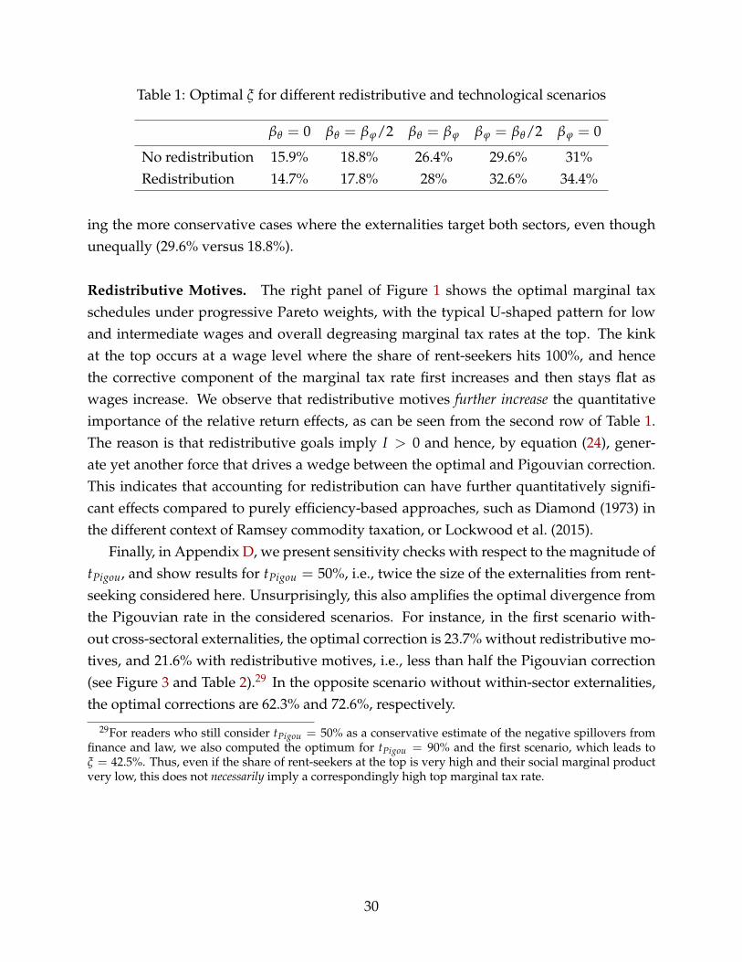
Table 1: Optimal ξ for different redistributive and technological scenarios

βθ = 0 βθ = βϕ/2 βθ = βϕ βϕ = βθ/2 βϕ = 0

No redistribution 15.9% 18.8% 26.4% 29.6% 31%Redistribution 14.7% 17.8% 28% 32.6% 34.4%

ing the more conservative cases where the externalities target both sectors, even thoughunequally (29.6% versus 18.8%).

Redistributive Motives. The right panel of Figure 1 shows the optimal marginal taxschedules under progressive Pareto weights, with the typical U-shaped pattern for lowand intermediate wages and overall degreasing marginal tax rates at the top. The kinkat the top occurs at a wage level where the share of rent-seekers hits 100%, and hencethe corrective component of the marginal tax rate first increases and then stays flat aswages increase. We observe that redistributive motives further increase the quantitativeimportance of the relative return effects, as can be seen from the second row of Table 1.The reason is that redistributive goals imply I > 0 and hence, by equation (24), gener-ate yet another force that drives a wedge between the optimal and Pigouvian correction.This indicates that accounting for redistribution can have further quantitatively signifi-cant effects compared to purely efficiency-based approaches, such as Diamond (1973) inthe different context of Ramsey commodity taxation, or Lockwood et al. (2015).

Finally, in Appendix D, we present sensitivity checks with respect to the magnitude oftPigou, and show results for tPigou = 50%, i.e., twice the size of the externalities from rent-seeking considered here. Unsurprisingly, this also amplifies the optimal divergence fromthe Pigouvian rate in the considered scenarios. For instance, in the first scenario with-out cross-sectoral externalities, the optimal correction is 23.7% without redistributive mo-tives, and 21.6% with redistributive motives, i.e., less than half the Pigouvian correction(see Figure 3 and Table 2).29 In the opposite scenario without within-sector externalities,the optimal corrections are 62.3% and 72.6%, respectively.

29For readers who still consider tPigou = 50% as a conservative estimate of the negative spillovers fromfinance and law, we also computed the optimum for tPigou = 90% and the first scenario, which leads toξ = 42.5%. Thus, even if the share of rent-seekers at the top is very high and their social marginal productvery low, this does not necessarily imply a correspondingly high top marginal tax rate.

30

6 Conclusion and Discussion

Our results are driven by the fact that income taxes are an imperfect instrument for cor-recting rent-seeking externalities. Directly taxing the externality-causing rent-seeking ac-tivity, were it possible, would reduce both its absolute desirability and its desirabilityrelative to other activities. By contrast, an income tax directly affects only the absolutedesirability of rent-seeking. The magnitude of the optimal correction via the income taxdepends, however, on the direction of the indirect (general equilibrium) effects of taxeson the relative desirability of rent-seeking. When within-activity externalities dominate,these indirect effects are perverse: higher taxes on portions of the income distributionwith high levels of rent-seeking raise the relative returns to rent-seeking and encourage ashift towards these activities. Consequently, the optimal externality correction lies strictlybelow the Pigouvian correction. When across-activity externalities dominate, the indirecteffects reinforce the direct effects, and the optimal correction strictly exceeds the Pigou-vian one.

We conclude by discussing a few additional considerations that may be important inpolicy applications.

Information Requirements. We demonstrated the potential quantitative importance ofgeneral equilibrium effects and, more generally, how our analytical results can be opera-tionalized to help inform the optimal design of income tax systems. Operationalizing ourresults requires taking a stand on (i) the magnitude of the rent-seeking externalities in theeconomy—and the distribution of rent-seeking across income levels—and (ii) the relativeimpact of these externalities on rent-seeking versus traditional activities. Our results sug-gest that both the level and relative impacts of rent-seeking externalities are likely to bequantitatively important. These are not well-known or easy-to-obtain quantities though:We know little or nothing about the relative impacts of rent-seeking externalities, and,while we benchmarked the overall magnitude of the externalities to the literature, sub-stantial additional research is needed to pin it down with a higher degree of confidence.We view our analysis as pointing to the importance of such research for income tax pol-icy, similar, for instance, to the work by economists and scientists on the magnitude anddistributional impacts of environmental externalities.

Taste Heterogeneity. In our model, individuals’ effort choices are driven exclusively bypecuniary concerns. In the full-specialization model described in the main text, for in-stance, individuals choose whether to be rent-seekers or traditional workers based purelyon the wages they can earn in those two sectors. It is straightforward, however, to in-troduce an extra “distaste for rent-seeking effort” parameter in our framework. If, per

31

Lockwood and Weinzierl (2015), this parameter affects preferences over effort and con-sumption in the same way as skills do, then these two parameters can be collapsed intoa single “effective skill” parameter to which all of our analysis directly applies.30 AsLockwood and Weinzierl emphasize, however, one needs, in this case, to be careful inhow one interprets Pareto weights over these effective skills: if, e.g., a primary driverof income differences is differences in the distaste-for-rent-seeking parameter—with low-distaste individuals earning high incomes in rent-seeking and high-distaste individualsearning lower incomes in traditional work—one might want to employ more stronglyprogressive Pareto weights than if differences were driven by skill alone.

Targeting. Our starting point is the assumption that rent-seeking income cannot bedirectly targeted, which is, of course, what makes our theoretical analysis non-trivial.Our results for this natural benchmark case can be interpreted as a cautionary assessmentof the ability of income taxes to substitute for targeted taxes, even if one could perfectlypinpoint the incomes at which rent-seeking predominates.

The extent to which the imperfect targeting assumption is justified differs somewhatacross applications. In our calibrated model in Section 5, it means that tax instruments arerestricted not to be occupation-specific. This may be because differential taxation createsadditional distortions if individuals can relabel their occupations, because it encouragesspecial interest lobbying for preferential tax treatment of particular occupations, or be-cause it raises concerns about horizontal equity and about empowering the governmentto make the determination of how socially productive workers in different professionsare. In other applications, for instance when individuals simultaneously pursue both tra-ditional and rent-seeking effort—as in our Ramsey model—it is even more natural to as-sume that individuals’ total incomes but not their rent-seeking shares are observable, be-cause the government would otherwise be required to collect detailed information aboutthe kind of tasks that individuals do, which is likely difficult and costly.

Regulation. We take the rent-seeking opportunities and hence externalities as given.Presumably, the government can also affect rents through regulation, which would affectthe form of the externalities through our technological return functions rθ(E) and rϕ(E)directly. However, as long as some rent-seeking opportunities remain after regulation,our analysis of optimal taxes applies, taking the degree of regulation as given.

30This sort of heterogeneity in the disutility from effort in different sectors is natural in our intensive-effort-margin Mirrleesian setting. This is different from the sort of fixed costs, unrelated to effort, consideredin Lockwood et al. (2015)’s extensive margin model.

32

References

Acemoglu, D., and D. Autor (2011): “Skills, Tasks and Technologies: Implications for

Employment and Earnings,” in Handbook of Labor Economics, ed. by D. Card, and O. Ashen-

felter. Elsevier.

Acemoglu, D., and T. Verdier (1998): “Property Rights, Corruption and the Allocation

of Talent: A General Equilibrium Approach,” Economic Journal, 108, 1381–1403.

Ales, L., M. Kurnaz, and C. Sleet (2015): “Tasks, Talents, and Taxes,” American Eco-

nomic Review, 105, 3061–3101.

Baker, G. (1992): “Incentive Contracts and Performance Measurement,” Journal of Po-

litical Economy, 100, 98–114.

Baumol, W. (1990): “Entrepreneurship: Productive, Unproductive, and Destructive,”

Journal of Political Economy, 98, 893–921.

Beaudry, P., C. Blackorby, and D. Szalay (2009): “Taxes and Employment Subsidies in

Optimal Redistribution Programs,” American Economic Review, 99, 216–242.

Bertrand, M., and S. Mullainathan (2001): “Are CEOs rewarded for luck?,” Quarterly

Journal of Economics, 116, 901–932.

Besley, T., and M. Ghatak (2013): “Bailouts and the Optimal Taxation of Bonus Pay,”

American Economic Review, Papers and Proceedings, 103, 163–167.

Cahuc, P., and E. Challe (2012): “Produce or Speculate? Asset Bubbles, Occupational

Choice and Efficiency,” International Economic Review, 53, 1105–1131.

Choné, P., and G. Laroque (2010): “Negative Marginal Tax Rates and Heterogeneity,”

American Economic Review, 100, 2532–2547.

Clarke, F. (1976): “A New Approach to Lagrange Multipliers,” Mathematics of Opera-

tions Research, 1, 165–174.

Colombi, R. (1990): “A New Model of Income Distributions: The Pareto Lognormal

Distribution,” in Income and Wealth Distribution, Inequality and Poverty, ed. by C. Dagum,

and M. Zenga, pp. 18–32. Springer, Berlin.

Cremer, H., F. Gahvari, and N. Ladoux (1998): “Externalities and Optimal Income

Taxation,” Journal of Public Economics, 70, 343–364.

Diamond, P. (1973): “Consumption Externalities and Imperfect Corrective Pricing,”

Bell Journal of Economics and Management Science, 4, 526–538.

Diamond, P. (1998): “Optimal Income Taxation: An Example with a U-shaped Pattern

of Optimal Tax Rates,” American Economic Review, 88, 83–95.

33

Dixit, A. (1985): “Tax Policy in Open Economies,” in Handbook of Public Economics, ed.

by A. Auerbach, and M. Feldstein, pp. 2475–2490. North Holland, Amsterdam.

French, K. (2008): “The Cost of Active Investing,” Journal of Finance, 63, 1537–1573.

Fudenberg, D., and J. Tirole (1991): Game Theory. MIT Press, Cambridge.

Golosov, M., P. Maziero, and G. Menzio (2013): “Taxation and Redistribution of

Residual Income Inequality,” Journal of Political Economy, 121, 1160–1204.

Heathcote, J., F. Perri, and G. Violante (2010): “Unequal we stand: An empirical anal-

ysis of economic inequality in the United States, 1967-2006,” Review of Economic Dynamics,

13, 15–51.

Holmström, B., and P. Milgrom (1991): “Multitask Principal-Agent Analyses: Incen-

tive Contracts, Asset Ownership, and Job Design,” Journal of Law, Economics, and Organi-

zation, 7, 24–52.

Hungerbuhler, M., E. Lehmann, A. Parmentier, and B. Linden (2008): “Optimal redis-

tributive taxation in a search equilibrium model,” Review of Economic Studies, 73, 743–767.

Kleven, H. J., C. T. Kreiner, and E. Saez (2009): “The Optimal Income Taxation of

Couples,” Econometrica, 77, 537–560.

Kopczuk, W. (2003): “A Note on Optimal Taxation in the Presence of Externalities,”

Economics Letters, 80, 81–86.

Lockwood, B., C. Nathanson, and G. Weyl (2015): “Taxation and the Allocation of

Talent,” Mimeo, Harvard University and University of Chicago.

Lockwood, B., and M. Weinzierl (2015): “De Gustibus non est Taxandum: Hetero-

geneity in preferences and optimal redistribution,” Journal of Public Economics, 124, 74–80.

Mirrlees, J. (1971): “An Exploration in the Theory of Optimum Income Taxation,”

Review of Economic Studies, 38, 175–208.

Murphy, K., A. Shleifer, and R. Vishny (1991): “The Allocation of Talent: Implications

for Growth,” Quarterly Journal of Economics, 106, 503–530.

Philippon, T. (2010): “Financiers versus Engineers: Should the Financial Sector be

Taxed or Subsidized?,” American Economic Journal: Macroeconomics, 2, 158–182.

Piketty, T., E. Saez, and S. Stantcheva (2014): “Optimal Taxation of Top Labor In-

comes: A Tale of Three Elasticities,” American Economic Journal: Economic Policy, 6, 230–

271.

Ramsey, F. (1927): “A Contribution to the Theory of Taxation,” Economic Journal, 37,

47–61.

Rochet, J.-C., and P. Choné (1998): “Ironing, Sweeping and Multidimensional Screen-

34

ing,” Econometrica, 66, 783–826.

Rothschild, C., and F. Scheuer (2011): “Optimal Taxation with Rent-Seeking,” NBER

Working Paper 17035.

————— (2013): “Redistributive Taxation in the Roy Model,” Quarterly Journal of

Economics, 128, 623–668.

————— (2014): “A Theory of Income Taxation under Multidimensional Skill Het-

erogeneity,” Mimeo, Wellesley College and Stanford University.

Roy, A. (1951): “Some Thoughts on the Distribution of Earnings,” Oxford Economic

Papers, 3, 135–146.

Sadka, E. (1978): “On the Optimal Taxation of Consumption Externalities,” Quarterly

Journal of Economics, 92.

Saez, E. (2001): “Using Elasticities to Derive Optimal Tax Rates,” Review of Economic

Studies, 68, 205–229.

Saez, E., J. Slemrod, and S. Giertz (2012): “The Elasticity of Taxable Income with

Respect to the Marginal Tax Rate,” Journal of Economic Literature, 50.

Sandmo, A. (1975): “Optimal taxation in the presence of externalities,” The Swedish

Journal of Economics, 77, 86–98.

Scheuer, F. (2013): “Adverse Selection in Credit Markets and Regressive Profit Taxa-

tion,” Journal of Economic Theory, 148, 1333–1360.

————— (2014): “Entrepreneurial Taxation with Endogenous Entry,” American Eco-

nomic Journal: Economic Policy, 6, 126–163.

Stiglitz, J. (1982): “Self-Selection and Pareto Efficient Taxation,” Journal of Public Eco-

nomics, 17, 213–240.

Werning, I. (2000): “An Elementary Proof of Positive Optimal Marginal Tax Rates,”

Mimeo, MIT.

————— (2007): “Pareto-Efficient Income Taxation,” Mimeo, MIT.

A Appendix: Proofs for Section 2

While we treat the elasticities βθ , βϕ, and σ as constants in the main text, it will be clear that from thefollowing proofs that the results extend trivially to the case where all three depend on E (in which case theregularity condition σ∆ > −1 + βθ must hold uniformly for all relevant E). The following proofs only relyon m(eθ , eϕ) being linear-homogeneous and weakly quasiconvex.

35

A.1 Proof of Lemma 1We first show that there is a unique equilibrium (t(E), T(E), E, Eθ(E)) associated with any E > 0. (Thisstep does not depend on the regularity condition σ∆ > −1 + βθ .) Second, we show that the regularitycondition implies the co-monotonicity, with E, of Eθ , l = m(Eθ , Eϕ), and Y, and the inverse wage 1/wE. Theco-monotonicity 1− t follows easily: 1− t = −ul/(wEuc) by the consumer’s problem (6), and −ul/uc isincreasing along any upward sloping locus when leisure and consumption are normal goods.

For the first step, note from the necessary and sufficient first-order conditions of the agent’s problem(3) first that rθ(E)

rϕ(E)=

mθ(x, 1)mϕ(x, 1)

, (27)

where x ≡ Eθ/E, mθ and mϕ denote the partial derivatives of m, and second that

t = 1 +ul(Y(Eθ , E), m(Eθ , E))mθ(Eθ , E)

uc(Y(Eθ , E), m(Eθ , E))rθ(E). (28)

Differentiating the log of the left-hand side of (27) with respect to E yields (omitting arguments)

rθ

rϕ

(r′θrθ−

r′ϕrϕ

)=

rθ

rϕ∆/E. (29)

Differentiating the log of the right-hand side w.r.t. x yields

1x

mθ

mϕ

(mθθ xmθ−

mθϕxmϕ

)=

mθ

mϕ

1σx

> 0, (30)

where we used the definition of the substitution elasticity σ = d log x/d log(mθ/mϕ). If ∆ = 0, the left-hand-side of (27) is constant, so (27) determines a unique x, and Eθ = Ex. If ∆ 6= 0, then, from (29) and (30),

dxdE

Ex= ∆σ. (31)

Hence, (27) implies a unique solution x(E) and Eθ(E) ≡ Ex(E) for any E. Substituting Eθ(E) for Eθ in (28)yields the unique tax t(E) consistent with an equilibrium with E. Budget balance pins down the uniqueassociated transfer T(E). This completes the first step.

For the second step, note that Eθ = xE. By (31), dEθdE

EEθ

= 1 + ∆σ > 1 + ∆σ− βθ > 0, so Eθ and E areco-monotonic. Similarly, l = m(Eθ , E) = Em(x, 1). Hence,

dldE

El= 1 +

mθ(x, 1)xm(x, 1)

dxdE

Ex= 1 +

mθ(x, 1)xm(x, 1)

∆σ. (32)

If ∆ ≥ 0, this is clearly positive. Otherwise, it exceeds 1 + ∆σ > 0 since

mθ(x, 1)xm(x, 1)

=mθ(x, 1)x

xmθ(x, 1) + mϕ(x, 1)∈ (0, 1).

Again similarly, Yθ = kθEθE−βθϕ , so

dYθ

dEEYθ

= 1 + ∆σ− βθ > 0. (33)

Since Y = Yθ + kϕE1−β, Y and E are co-monotonic. Finally, wE is the maximum over x of (rθ(E)x +

36

rϕ(E))/m(x, 1), which is decreasing in E (since the returns rθ , rϕ are decreasing in E at each x). So 1/wE isco-monotonic with E.

A.2 Proof of Proposition 1Using the formulas in the proof of Lemma 1, it is straightforward to show that E→ 0 implies l → 0, Y → 0,and 1/wE → 0. We can also use Lemma 1 to write the planner’s problem in terms of l as maxl u (Y(l), l). Theplanner’s objective is increasing/locally constant/decreasing in l if and only if (suppressing arguments)

uc

(dYdl

+uluc

)R 0. (34)

Using wE = Y/l yieldswEuc

(dYdl

lY+

1wE

uluc

)R 0. (35)

Next, write Y(l) = Y(E(l)x(E(l)), E(l)) and compute

dYdl

Yl=

(dYdE

EY

)(dEdl

lE

)=

(∂Y∂E

+∂Y∂Eθ

(E

dxdE

+ x))

EY

(dEdl

lE

)=

((1− tPigou)rϕ

EY+ (1− s)

YEθ

x(1 + ∆σ)EY

)(1 +

mθ(x, 1)xm(x, 1)

∆σ

)−1

=((1− tPigou)s + (1− s)(1 + ∆σ)

)(1 + (1− s)∆σ)−1

=(s(1− βϕ) + (1− s)(1 + ∆σ− βθ)

)(1 + (1− s)∆σ)−1 (36)

where we used ∂Y/∂Eθ = rθ = (1− s)Y/Eθ , the definition of tPigou in (2), expressions (31) and (33), and thefact that wEmθ(x, 1) = rθ from the agent’s problem.

Combining (36) and (35) shows that the planner’s objective is increasing/locally constant/decreasingin l as [

s(1− βϕ) + (1− s)(1 + ∆σ− βθ)](1 + (1− s)∆σ)−1 R − 1

wE

uluc

. (37)

Since 1/wE → 0 and (by assumption) −ul/uc → 0 as E→ 0, while

s(1− βϕ) + (1− s)(1 + ∆σ− βθ) ≥ min{

1− βϕ, 1 + ∆σ− βθ

}> 0

and (1 + (1− s)∆σ) ∈ (0, 1 + |∆σ|), we see that the planner’s objective is increasing in l as l → 0. We cantherefore find a sufficiently small l0 such that the planer’s objective is increasing in l at l0. We next showthat there exists an l1 such that the planner’s objective u(Y(l), l) < u(Y(l0), l0) ∀l > l1. The existence of anoptimum will then follow from the facts that [l0, l1] is compact and the equilibrium locus and the planner’sobjective are continuous.

Towards constructing l1, consider the agent’s indifference curve in (l, c)-space through (l0, Y0). It isstrictly convex and has slope −ul(Y(l0), l0)/uc(Y(l0), l0) > 0 at (l0, Y(l0)). Hence, along the indifferencecurve, the ratio c/l is bounded below by −ul(Y(l0), l0)/uc(Y(l0), l0) > 0 as (l, c) grows large. On the otherhand, the ratio Y(l)/l = w(l)→ 0 along the equilibrium locus. So there exists an l1 sufficiently high so thatthe indifference curve lies strictly above the equilibrium locus.

Finally, to obtain the optimal tax formula (8) and complete the proof, note that a necessary conditionfor the planner’s optimum is that (35) holds with equality. Using (36) and the fact, from the agent’s opti-

37

mization problem, that (1− t)w = −ul/uc, yields

1− t =((1− tPigou)s + (1− s)(1 + ∆σ)

)(1 + (1− s)∆σ)−1 . (38)

Rearranging yields (8).

A.3 Details on Section 2.4 and Proof or Corollary 1Using the functional forms for the returns and preferences, we can write (27) and (28) as x = E∆σ(kθ/kϕ)σ

and

(1− t)kϕE−βϕ = e1εϕ

(1 + x

1+σσ

) σ−εε(1+σ) .

Using eϕ = E and the first condition to write E as a function of x in the second condition, we obtain

1− t = k− 1+εβϕ

∆εθ k

1+εβϕ−∆ε

∆εϕ x

1+εβϕε∆σ

(1 + x

1+σσ

) σ−εε(1+σ) .

Finally, note that

s =Yϕ

Y=

kϕE1−βϕ

kθEθE−βθ + kϕE1−βϕ=

(1 +

kθ xE1−βθ

kϕE1−βϕ

)−1

=

(1 +

kθ

kϕxE∆

)−1=(

1 + x1+σ

σ

)−1.

Using this above to substitute s for x delivers equation (10) in the main text, with K ≡ k− 1+εβϕ

∆εθ k

1+εβϕ−∆ε

∆εϕ .

To prove Corollary 1, note that an optimal equilibrium is an intersection of the two functions topt(s)and teq(s), where the former is given by the right-hand side of (9) and the latter is given by 1 minus theright-hand side of (10), for any s ∈ [0, 1].

As for the former, in the limit as σ → ∞, topt(s) is identically 0 for s ∈ [0, 1) if ∆ > 0. Moreover,topt(1) = βϕ for all σ. As for the latter, if ∆ > 0, teq(s) converges on s ∈ (0, 1) to the increasing limit functionteq

(s) = 1− Ks−1/ε. For s→ 0, teq(s)→ −∞ and for s→ 1, teq

(s)→ 1− K.If K < 1− βϕ, comparing the limit points of the graphs of the functions teq

(s) and topt(s) as σ → ∞

shows that, for sufficiently large σ, there must be a unique s(σ) for which teq(s(σ)) = teq

(s(σ)), and thisunique intersection, which is the optimum, must satisfy s(σ)→ K1/ε ∈ (0, 1) and teq

(s(σ))→ 0.

B Appendix: Proofs for Section 3In this appendix, we show how our analysis from Section 3.2 extends to the case where the effort aggregatorm is quasiconvex and linear homogeneous, which allows for the linear m case discussed in the main text asa special case. We again characterize a direct implementation, where individuals announce their privatelyknown type (θ, ϕ) and then get assigned c(θ, ϕ), y(θ, ϕ), and the fraction of income earned through theΘ-activity, given by q(θ, ϕ) ≡ yθ(θ, ϕ)/y(θ, ϕ) = rθ(E)θeθ(θ, ϕ)/y(θ, ϕ). Income y and consumption c areobservable but an individual’s skill type (θ, ϕ) and the activity-specific efforts eθ or eϕ (and q) are not. The

38

resulting incentive constraints that guarantee truth-telling of the agents are:

u(

c(θ, ϕ), m(

q(θ, ϕ)y(θ, ϕ)

θrθ(E),(1− q(θ, ϕ))y(θ, ϕ)

ϕrϕ(E)

))≥ max

p∈[0,1]

{u(

c(θ′, ϕ′), m(

py(θ′, ϕ′)

θrθ(E),(1− p)y(θ′, ϕ′)

ϕrϕ(E)

))}∀(θ, ϕ), (θ′, ϕ′), (39)

since type (θ, ϕ) can imitate another type (θ′, ϕ′) by earning (θ′, ϕ′)’s income using a continuum of combi-nations of efforts (and thus income shares (p, 1− p)) in the Θ- and Φ-activities.

The following lemma shows that incentive compatibility implies that each type (θ, ϕ) has a well-definedwage w ≡ y/l and activity-specific income share q, which both depend on aggregate rent-seeking effort Ebut are otherwise independent of the allocation.

Lemma 4. In any incentive compatible allocation {c(θ, ϕ), y(θ, ϕ), q(θ, ϕ), E},

w(θ, ϕ) ≡ y(θ, ϕ)

l(θ, ϕ)= max

p∈[0,1]m(

pθrθ(E)

,1− p

ϕrϕ(E)

)−1(40)

and q(θ, ϕ) is a corresponding arg max.

Proof. By the linear homogeneity of m, the “own type” incentive constraints (for (θ, ϕ) = (θ′, ϕ′)) imply

q(θ, ϕ) ∈ argminp∈[0,1]

m(

py(θ, ϕ)

θrθ(E),(1− p)y(θ, ϕ)

ϕrϕ(E)

)= argmin

p∈[0,1]m(

pθrθ(E)

,1− p

ϕrϕ(E)

).

Equation (40) then follows immediately from the definitions w(θ, ϕ) ≡ y(θ, ϕ)/l(θ, ϕ) and

l(θ, ϕ) ≡ m(eθ(θ, ϕ), eϕ(θ, ϕ)) = y(θ, ϕ)m(

q(θ, ϕ)θrθ(E) , 1− q(θ, ϕ)

ϕrϕ(E)

).

By Lemma 4, fixing E pins down each type’s wage wE(θ, ϕ), as in (5). Moreover, q(θ, ϕ) is chosen tominimize the overall effort m(eθ , eϕ) subject to achieving a given amount of income. When m is strictlyquasiconvex, q(θ, ϕ), which depends only on the skill ratio α ≡ θ/ϕ, is also uniquely determined by E foreach α. With weakly quasiconvex m, q(θ/ϕ) is uniquely determined outside of a countable set of α-values,where it is interval-valued because the individual is indifferent between various effort combinations toachieve a given income. By Lemma 4, the correspondence q(θ/ϕ) depends on, and is non-decreasing in,the relative returns ζE(α) ≡ αrθ(E)/rϕ(E), and we can define the functions qE(α) ≡ Q(ζE(α)) by taking q tobe equal to the midpoints of the intervals on the countable set of degenerate α’s.

Viewed as a distribution, Q has a well-defined derivative denoted by Q′.31 Since

x =eθ

eϕ=

ϕrϕ(E)θrθ(E)

(y

eϕ ϕrϕ(E)− 1)=

1ζE(α)

q1− q

, (41)

we can write Q(ζ) = ζx(ζ)/(1+ ζx(ζ)), which only depends on and is increasing in ζ by linear homogene-ity and quasiconvexity of m. For later use, it will also be helpful to define Qζ0(ζ) ≡ ζ0x(ζ)/(1 + ζ0x(ζ))

with Q′(ζ) ≡ Q′ζ0(ζ)∣∣∣ζ0=ζ

, i.e. the change in the traditional income share Q that is due to the change in the

activity-specific effort ratio x in response to a change in relative returns ζ, but holding ζ fixed otherwise.

31In particular, Q(ζ) is ordinarily differentiable except at some countable number of jump discontinuities;the latter adds a series of Dirac δ-functions to Q′. See Appendix C.3. Recall that q ∈ {0, 1} for almost allindividuals if m is linear, but otherwise will typically take interior values.

39

C Appendix: Proofs for Section 4

C.1 Wage Distributions for General mLemma 4 showed that fixing E determines the wage wE(θ, ϕ) and the traditional activity income share qE(α)

for each type (θ, ϕ). For any given E, we compute the cdf over (w, α)-pairs:

GE(w, α) ≡∫{(θ,ϕ)|wE(θ,ϕ)≤w, θ/ϕ≤α}

dF(θ, ϕ)

with the corresponding density gE(w, α). This allows us to obtain the wage distribution for any given Esimply as the marginal distribution

FE(w) ≡∫{(θ,ϕ)|wE(θ,ϕ)≤w}

dF(θ, ϕ) =∫ w

wE

∫ ∞

α=0dGE(z, α)

with the corresponding density fE(w) =∫ ∞

α=0 dGE(w, α) as well as the activity-specific densities f θE(w) ≡∫ ∞

α=0 qE(α)dGE(w, α) and f ϕE (w) ≡

∫ ∞α=0(1− qE(α))dGE(w, α). Hence, these densities can be interpreted as

an average value of q (respectively 1− q) for all individuals at wage w, and fE(w) = f θE(w) + f ϕ

E (w) for allw ∈ [wE, wE]. In the special case with m(eθ , eϕ) = eθ + eϕ, (40) immediately implies qE(α) ∈ {0, 1} almosteverywhere, leading to the definitions in the main text.

C.2 Proof of Proposition 2Putting multipliers λ on (15), ξλ on (14) and η(w)λ on (13), the Lagrangian corresponding to (12)-(15) is,after integrating by parts (13),

L =∫ wE

wEV(w)ψE(w)dw−

∫ wEwE

V(w)η′(w)λdw +∫ wE

wEul(c(V(w), l(w)), l(w)) l(w)

w η(w)λdw

+ξλYϕ(E)− ξλ∫ wE

wEwl(w) f ϕ

E (w)dw + λ∫ wE

wEwl(w) fE(w)dw− λ

∫ wEwE

c(V(w), l(w)) fE(w)dw. (42)

By Theorem 3 in Clarke (1976), this Lagrangian approach is generically valid, i.e. constraint qualification issatisfied and any solution must be a stationary point of Lagrangian for some (bounded) multipliers. Using∂c/∂V = 1/uc and compressing notation, the first order condition for V(w) is

η′(w)λ = ψE(w)− λ fE(w)1

uc(w)+ η(w)λ

ulc(w)

uc(w)

l(w)

w. (43)

Defining η(w) ≡ η(w)uc(w), this becomes

η′(w) = ψE(w)uc(w)

λ− fE(w) + η(w)

ucc(w)c′(w) + ucl(w)l′(w) + ucl(w)l(w)/wuc(w)

. (44)

Using the first order condition corresponding to the incentive constraint (16),

uc(w)c′(w) + ul(w)l′(w) + ul(w)l(w)

w= 0, (45)

40

the fraction in (44) can be written as −(∂MRS(w)/∂c)y′(w)/w, where M(c, l) ≡ −ul(c, l)/uc(c, l) is themarginal rate of substitution between effort and consumption and MRS(w) ≡ M(c(w), l(w)), so (with aslight abuse of notation) ∂MRS(w)/∂c stands short for ∂M(c(w), l(w))/∂c. Substituting in (44) and rear-ranging yields

− ∂MRS(w)

∂cl(w)

y′(w)

y(w)η(w) = fE(w)− ψE(w)

uc(w)

λ+ η′(w). (46)

Integrating this ODE gives

η(w) =∫ wE

w

(fE(x)− ψE(x)

uc(x)λ

)exp

(∫ x

w

∂MRS(s)∂c

l(s)y′(s)y(s)

ds)

dx

=∫ wE

w

(1− ψE(x)

fE(x)uc(x)

λ

)exp

(∫ x

w

(1− εu(s)

εc(s)

)dy(s)y(s)

)fE(x)dx, (47)

where the last step follows from l(w)∂MRS(w)/∂c = 1 − εu(w)/εc(w) after tedious algebra (e.g. usingequations (23) and (24) in Saez, 2001).

Using ∂c/∂l = MRS, the first order condition for l(w) is

λw fE(w)

(1− MRS(w)

w

)− ξλw f ϕ

E (w) = −η(w)λ

[(−ulc(w)ul(w)/uc(w) + ull(w)) l(w)

w+

ul(w)

w

],

which after some algebra can be rewritten as

w fE(w)

(1− MRS(w)

w

)− ξw f ϕ

E (w) = η(w)

(∂MRS(w)

∂llw

+MRS(w)

w

), (48)

where ∂MRS(w)/∂e again stands short for ∂M(c(w), l(w))/∂l. With MRS(w)/w = 1− T′(y(w)) from thefirst-order condition of the workers, this becomes

1− ξf ϕE (w)

fE(w)= (1− T′(y(w)))

[1 +

η(w)

w fE(w)

(1 +

∂MRS(w)

∂ll

MRS(w)

)]. (49)

Simple algebra again shows that 1 + ∂ log MRS(w)/∂ log l = (1 + εu(w))/εc(w), so that the result followsfrom (47) and (49).

C.3 Proof of Lemma 3We prove the following lemma for the case of a general m-aggregator function. Lemma 3 will then emergeas a special case for linear m.

Lemma 5. The welfare effect of a marginal change in aggregate rent-seeking effort E is given by (19) in Lemma 3.The terms I and R are as in (20) and (21). C and S are given by

C ≡∫ wE

wE

w2l′(w)VarE(q|w) fE(w)dw (50)

andS ≡

∫ wE

wE

∫ ∞

α=0y(w)Q′(ζE(α))ζE(α)dGE(w, α) ≥ 0 (51)

with VarE(q|w) =∫ ∞

0 qE(α)2gE(α|w)dα−

(∫ ∞0 qE(α)gE(α|w)dα

)2 and gE(α|w) = gE(w,α)fE(w)

.

41

Before proving Lemma 5, we establish some preliminary results. Because we allow m to be only weaklyquasiconvex, the marginal rate of substitution χ(eθ/eϕ) ≡ mθ(eθ/eϕ)/ mϕ(eθ/eϕ) can have constant re-gions. Since χ is non-decreasing, there are at most a countable number of such regions. Use {di}n

i=1, with di

increasing in i, to denote the values of χ at these flat regions.32 An individual with θ/ϕ =rϕ(E)rθ(E) di ≡ αi

E will

be indifferent between a range of activity-specific income shares q ∈[qi, qi

], where, by equation (41), the

bounds are, respectively, the minimum and the maximum q for which χ(

q1−q

1di

)= di and thus indepen-

dent of E. The upper-hemicontinuous correspondence qE(α) thus jumps from qi to qi as α crosses αiE from

below. For any given wage w and E, taking α0E = θ/ϕ and αn+1

E = θ/ϕ, we can thus write33

FE(w) =∫ αn+1

E

α0E

∫ w

wE(α)gE(w′, α)dw′dα =

n

∑i=0

∫ αi+1E

αiE

∫ w

wE(α)gE(w′, α)dw′dα,

where wE(α) ≡ wE

(max{θ, αϕ}, max{θ/α, ϕ}

)and wE(α) ≡ wE

(min{θ, αϕ}, min{θ/α, ϕ}

). Similarly, we

can write

FθE(w) =

n

∑i=0

∫ αi+1E

αiE

∫ w

wE(α)qE(α)gE(w′, α)dw′dα.

The latter is a useful formulation because, on each of the intervals in the sum, the function qE(α) is contin-uously differentiable. The discontinuities occur at the boundaries of the intervals. It allows us to prove thefollowing technical lemma, which will be useful below.

Lemma 6.

dFE(w)

dE=

βϕ(E)E

w f ϕE (w) +

βθ(E)E

w f θE(w) and

dFθE(w)

dE=

βθ(E)E

w f θE(w)− KE(w)− LE(w), where (52)

KE(w) ≡ −n

∑i=0

∫ αi+1E

αiE

∫ w

wE(α)

dqE(α)

dEgE(w′, α)dw′dα +

n

∑i=1

∫ w

wE(αiE)

dαiE

dE

(qi − qi

)gE

(w′, αi

E

)dw′

= −∆(E)E

∫ αn+1E

α0E

∫ w

wE(α)Q′(ζE(α))ζE(α)gE(w′, α)dw′dα (53)

and LE(w) ≡ −∆(E)E

∫ αn+1E

α0E

qE(α)(1− qE(α))wgE(w, α)dα. (54)

Moreover, dFϕE (w)/dE = dFE(w)/dE− dFθ

E(w)/dE and analogous expressions hold for dΨE(w)/dE, dΨθE(w)/dE

and dΨϕE(w)/dE.

Proof. It is useful to define the function w(w, α, E; E0) as the wage, at E, of the type (θ, ϕ) that would havehad wage w (and α) at E = E0. Then, by construction, the set {(θ, ϕ)|wE(θ, ϕ) ≤ w(w, θ/ϕ, E; E0)} is in-dependent of E: it is simply the set of types that would have had wage less than w at E0. Hence, for allE,

FE0(w) =∫ αn+1

E

α=α0E

∫ w(w,α,E;E0)

wE(α)gE(w′, α)dw′dα (55)

32We deal with finite n to keep notation clean; the countably infinite case is an easy but notationallycumbersome extension.

33We mildly abuse notation here in assuming that α0E ≤ α1

E and αn+1E ≥ αn

E since a simple redefinition ofn and the relevant αi

E values would yield the same formulae.

42

i.e., the measure of types with wage less than w when E = E0. Taking the derivative of the RHS with respectto E (which is zero by construction) and evaluating at E0 and re-arranging yields

∫ αn+1E

α=α0E

∫ w

wE(α)

dgE0(w′, α)

dEdw′dα−

∫ αn+1E

α=α0E

dwE0(α)

dEgE0(wE0

, α)dα = −∫ αn+1

E

α=α0E

dw(w, α, E0; E0)

dEgE0(w, α)dα.

The LHS is easily recognized as dFE(w)/dE, evaluated at E0. Computing dw(w, α, E0; E0)/dE,

dFE(w)

dE=∫ αn+1

E

α=α0E

(qE(α)

βθ(E)E

w + (1− qE(α))βϕ(E)

Ew)

gE(w, α)dα =βθ(E)

Ew f θ

E(w) +βϕ(E)

Ew f ϕ

E (w),

which proves the first result in (52). Moreover, for all E,

FθE0(w) =

n

∑i=0

∫ αi+1E0

αiE0

∫ w(w,α,E;E0)

wE(α)qE0(α)gE(w′, α)dw′dα, (56)

since the set of types being integrated over is independent of E, and so is qE0(α). We explicitly compute thederivative with respect to E of the RHS of (56), which is zero since the object is, by construction, independentof E. After some re-arranging and evaluating at E0, we get

n

∑i=0

∫ αi+1E0

αiE0

∫ w

wE0(α)

qE0(α)dgE0(w

′, α)

dEdw′dα−

n

∑i=0

∫ αi+1E0

αiE0

dwE0(α)

dEqE0(α)gE0

(wE0

(α), α)

dα

= −n

∑i=0

∫ αi+1E0

αiE0

dw(w, α, E0; E0)

dEqE0(α)gE0(w, α)dα. (57)

Adding ∑ni=0∫ αi+1

E0αi

E0

∫ wwE0

(α)

dqE0 (α)

dE gE0(w′, α)dw′dα−∑n

i=1∫ w

wE0(αi

E0)

dαiE0

dE

(qi − qi

)gE0

(w′, αi

E0

)dw′ to both sides,

we can recognize the left hand side as dFθE(w)/dE evaluated at E0. Again substituting for dw(w, α, E0; E0)/dE,

the RHS of (57) is

∫ αn+1E

α0E

(qE0(α)

βθ(E0)

E0w + (1− qE0(α))

βϕ(E0)

E0w)

qE0(α)gE0(w, α)dα

=βθ(E0)

E0w f θ

E0(w) +

∆(E0)

E0

∫ αn+1E

α0E

qE0(α)(1− qE0(α))wgE0(w, α)dα.

Using the definitions in (53) and (54), we conclude that dFθE(w)/dE = βθ(E)

E w f θE(w)− KE(w)− LE(w).

Finally, observe that qE(α) ≡ qE(α)− ∑ni=1(q

i − qi)H(α− αiE), where H is the Heaviside step function

(using the half-maximum convention), is continuous. It has a well-defined derivative with respect to Eequal to dqE(α)/dE away from the αi

E-jumps, and well-defined (bounded) left- and right-derivatives at thejumps. Therefore,∫ αn+1

E

α=α0E

∫ w

wE(α)

dqE(α)

dEgE(w′, α)dw′dα =

n

∑i=0

∫ αi+1E

α=αiE

∫ w

wE(α)

dqE(α)

dEgE(w′, α)dw′dα. (58)

43

Differentiating H as a distribution yields dH(α−αiE)

dE = −δ(α− αiE)

dαiE

dE , where δ is the Dirac δ-function. Hence,

∫ αn+1E

α=α0E

∫ w

wE(α)(qi − qi)

dH(α− αiE)

dEgE(w′, α)dw′dα = −

∫ w

wE(αiE)

dαiE

dE(qi − qi)gE(w′, αi

E)dw′. (59)

Combining (58) and (59) (and differentiating qE(α) as a distribution), we have

∫ αn+1E

α=α0E

∫ w

wE(α)

dqE(α)

dEgE(w′, α)dw′dα =

n

∑i=0

∫ αi+1E

α=αiE

∫ w

wE(α)

dqE(α)

dEgE(w′, α)dw′dα−

n

∑i=0

∫ w

wE(αiE)

dαiE

dE(qi − qi)gE(w′, αi

E)dw′.

Using Q(ζE(α)) ≡ qE(α) and dζE(α)/dE = ζE(α)∆(E)/E yields the second equality in (53).

Lemma 6 will be used in the now following proof of Lemma 5. Using (42) and a standard envelopetheorem,

W ′(E) =∫ wE

wE

V(w)dψE(w)

dEdw− λ

∫ wE

wE

c(V(w), l(w))d fE(w)

dEdw

+ λ(1− ξ)∫ wE

wE

wl(w)d f ϕ

E (w)

dEdw + λ

∫ wE

wE

wl(w)d f θ

E(w)

dEdw + ξλY′ϕ(E) + B1 (60)

with

B1 ≡dwEdE

[V(wE)ψE(wE)− λc(V(wE), l(wE)) fE(wE) + λ

(fE(wE)− ξ f ϕ

E (wE))

wEe(wE)]

−dwEdE

[V(wE)ψE(wE)− λc(V(wE), l(wE)) fE(wE) + λ

(fE(wE)− ξ f ϕ

E (wE))

wEe(wE)]

and Yϕ(E) ≡ rϕ(E)E. Integrating by parts the four integrals yields

W ′(E) = B1 + B2 −∫ wE

wE

V′(w)dΨE(w)

dEdw + λ

∫ wE

wE

(V′(w)

uc(w)+ MRS(w)l′(w)

)dFE(w)

dEdw

− λ(1− ξ)∫ wE

wE

(wl′(w) + l(w))dFϕ

E (w)

dEdw− λ

∫ wE

wE

(wl′(w) + l(w))dFθ

E(w)

dEdw + ξλY′ϕ(E) (61)

with

B2 =

[V(w)

dΨE(w)

dE− λc(V(w), l(w))

dFE(w)

dE+ λ(1− ξ)wl(w)

dFϕE (w)

dE+ λwl(w)

dFθE(w)

dE

]wE

wE

.

By the first order conditions (46) and (48) with respect to V(w) and l(w) from the inner problem, the terms

A1(E) ≡ λ∫ wE

wE

l′(w)

fE(w)

[w fE(w)

(1− MRS(w)

w

)− ξw f ϕ

E (w)− η(w)

(∂MRS(w)

∂ll(w)

w+

MRS(w)

w

)]dFE(w)

dEdw

and A2(E) ≡ λ∫ wE

wE

V′(w)

uc(w) fE(w)

[ψE(w)

uc(w)

λ− fE(w)− η′(w)− η(w)

∂MRS(w)

∂cl(w)

y′(w)

y(w)

]dFE(w)

dEdw

44

are both equal to zero. Adding A1(E) and A2(E) to (61), using (13) and re-arranging yields

W ′(E) = B1 + B2 + ξλY′ϕ(E) +∫ wE

wE

V′(w)

(ψE(w)

fE(w)

dFE(w)

dE− dΨE(w)

dE

)dw

− λ∫ wE

wE

l(w)dFE(w)

dEdw + ξλ

∫ wE

wE

((l(w) + wl′(w))

dFϕE (w)

dE− wl′(w)

f ϕE (w)

fE(w)

dFE(w)

dE

)dw

− λ∫ wE

wE

(η(w)

wd [MRS(w)l(w)]

dw+ η′(w)

V′(w)

uc(w)

)1

fE(w)

dFE(w)

dEdw. (62)

Using Lemma 6, the first integral in (62) is

∆(E)E

∫ wE

wE

V′(w)wf θE(w) f ϕ

E (w)

fE(w)

(ψθ

E(w)

f θE(w)

−ψ

ϕE(w)

f ϕE (w)

)dw =

∆(E)E

R (63)

Again using Lemma 6, the terms with l(w) in the second line of (62) can be written as

−λ(1− ξ)βϕ(E)

E

∫ wE

wE

wl(w) f ϕE (w)dw− λ

βθ(E)E

∫ wE

wE

wl(w) f θE(w)dw + ξλ

∫ wE

wE

l(w)(KE(w) + LE(w))dw

= −λ

(βϕ(E)rϕ(E) + βθ(E)

rθ(E)E

Eθ

)+ ξλβϕ(E)rϕ(E) + ξλ

∫ wE

wE

l(w)(KE(w) + LE(w))dw

= −λrϕ(E)tPigou + ξλβϕ(E)rϕ(E) + ξλ∫ wE

wE

l(w)(KE(w) + LE(w))dw. (64)

The terms with wl′(w) in (62) can be written as

ξλ∫ wE

wE

wl′(w)

[βϕ(E)

Ew f ϕ

E (w)−f ϕE (w)

fE(w)

wE

(βϕ(E) f ϕ

E (w) + βθ(E) f θE(w)

)+ KE(w) + LE(w)

]dw

= ξλ∆(E)

E

∫ wE

wE

w2l′(w)

[f θE(w) f ϕ

E (w)

fE(w)−∫ ∞

0qE(α)(1− qE(α))gE(w, α)dα

]dw + ξλ

∫ wE

wE

wl′(w)KE(w)dw

= ξλ∆(E)

E

∫ wE

wE

w2l′(w)VarE(q|w) fE(w)dw + ξλ∫ wE

wE

wl′(w)KE(w)dw

= ξλ∆(E)

EC + ξλ

∫ wE

wE

wl′(w)KE(w)dw, (65)

where the first equality uses (54). Combining the terms with KE(w) from (64) and (65) gives ξλ∫ wE

wE(wl(w))′KE(w)dw,

which can be integrated by parts to yield

B3 − ξλ∫ wE

wE

wl(w)K′E(w)dw = B3 + ξλ∆(E)

E

∫ wE

wE

∫ ∞

0y(w)Q′(ζE(α))ζE(α)dGE(w, α) (66)

with B3 = ξλwEl(wE)KE(wE) since KE(wE) = 0. Further combining this with the LE(w)-term in (64) yields

B3 + ξλ∆(E)

E

∫ wE

wE

y(w)∫ ∞

0

(Q′(ζE(α))ζE(α)− qE(α)(1− qE(α))

)dGE(w, α). (67)

45

Note that Q′(ζ) = Q′ζ0(ζ)∣∣∣ζ0=ζ

= Q′(ζ)ζ −Q(ζ)(1−Q(ζ)), so that (67) becomes

B3 + ξλ∆(E)

E

∫ wE

wE

∫ ∞

0y(w)Q′(ζE(α))ζE(α)dGE(w, α) = B3 + ξλ

∆(E)E

S. (68)

Moreover, S ≥ 0 since Q′(ζ) = ζ2x′(ζ)/(1+ ζx(ζ))2 ≥ 0. Finally, use the incentive constraint (13), rewrittenas V′(w)/uc(w) = MRS(w)l(w)/w, to write the last line of (62) as

−λ∫ wE

wE

(η(w)w

d[V′(w)/uc(w)]

dw+ η′(w)w

V′(w)

uc(w)+ η(w)

V′(w)

uc(w)

)1

w fE(w)

dFE(w)

dEdw

or, recognizing the sum of the bracketed terms as d[η(w)wV′(w)/uc(w)]/dw, integrating by parts, andusing the transversality condition η(wE) = η(wE) = 0 and (52),

λ∫ wE

wE

η(w)wV′(w)

uc(w)

ddw

(βθ(E)

Ef θE(w)

fE(w)+

βϕ(E)E

f ϕE (w)

fE(w)

)dw

= λ∆(E)

E

∫ wE

wE

η(w)wV′(w)

uc(w)

ddw

(f ϕE (w)

fE(w)

)dw =

∆(E)E

I. (69)

Define F(w, E) ≡ FE(w). Since F(wE, E) ≡ 1 for all E,

dF(wE, E)dE

=∂F(wE, E)

∂E+

∂F(wE, E)∂w

dwEdE

=dFE(wE)

dE+ fE(wE)

dwEdE

= 0. (70)

Together with an analogous expression at wE and the fact that KE(wE) = LE(wE) = LE(wE) = 0, this yieldsB1 + B2 = −ξλwE l(wE)KE(wE) = −B3. Using (63), (64), (65), (68) and (69) in (62) yields

W ′(E) = −λrϕ(E)tPigou +∆(E)

E(R + I) + ξλ

(rϕ(E) +

∆(E)E

(C + S))

, (71)

where we have used Y′ϕ(E) + βϕ(E)rϕ(E) = rϕ(E). This completes the proof of Lemma 5.To see that Lemma 3 is implied as a special case when m is linear, observe that then n = 1, q1 = 1,

q1 = 0, s1 = 1, and α1E =

rϕ(E)rθ(E) . Hence, for the region where q = 1,

KE(w) =n

∑i=1

∫ w

wE

dαiE

dE(qi − qi)gE(w′, αi

E)dw′ =d

dE

(rϕ(E)rθ(E)

) ∫ w

wE

gE

(w′,

rϕ(E)rθ(E)

)dw′.

In this region, w = θrθ(E) and α = θ/ϕ. Hence, θ = w/rθ(E), ϕ = wαrθ(E) and the Jacobian for the

transformation is wα2rθ(E)2 . Therefore, gE

(w, rϕ(E)

rθ(E)

)= w

(α1E)

2rθ(E)2 f(

wrθ(E) , w

α1Erθ(E)

), or, transforming to ϕ =

w/rϕ(E),

KE(w) =d

dE

(rϕ(E)rθ(E)

) ∫ w

wE

gE

(w′,

rϕ(E)rθ(E)

)dw′ = −∆(E)

Erϕ(E)rθ(E)

∫ w/rϕ(E)

ϕϕ f(

ϕrϕ(E)rθ(E)

, ϕ

)dϕ.

Moreover, LE(w) = 0 since q ∈ {0, 1}. Using this in (65) and (66) yields the result.

46

C.4 Proof of Proposition 3The first part of the proposition is established by the following lemma:

Lemma 7. ξ > 0 in any regular Pareto optimum.

Proof. Any Pareto optimum solves maxE,T(.)∫ wE

wEu (yT(w)− T(yT(w)), yT(w)/w) dΨE(w) subject to (a) a

set of incentive constraints yT(w) ∈ arg maxy u(y − T(y), y/w) for all w, (b) the consistency constraintYϕ(E)−

∫ wEwE

yT(w) f ϕE (w)dw = 0 and (c) the revenue constraint

∫ wEwE

T(yT(w))dFE(w) ≥ 0. We show thatany solution to the relaxed problem where the consistency constraint (c) is replaced by the inequality con-straint Yϕ(E)−

∫ wEwE

yT(w) f ϕE (w)dw ≥ 0, with associated multiplier λξ, always has ξ > 0 with regular Ψ.

Since this implies that the solution (E∗, T∗(.)) to the relaxed problem is feasible in the unrelaxed problem,ξ = ξ > 0 as well. So, suppose, by way of contradiction, that ξ = 0 in (E∗, T∗(.)). Standard arguments(e.g. Werning, 2000) imply T∗′(.) ≥ 0 with regular Pareto weights in this case. Now consider a small de-crease ∆E from E∗ holding T∗(.) fixed. This at least weakly increases the wage, and hence the utility, ofeach individual, increasing the objective. It has no effect on the set of incentive constraints (a) since T∗(.)remains fixed. It has no effect on the relaxed constraint (b) since ξ = 0. It relaxes the revenue constraint (c)since yT(w) is non-decreasing and T∗′(.) ≥ 0. This contradicts the optimality of (E∗, T∗(.)) in the relaxedproblem, showing that ξ > 0 in the relaxed problem and hence ξ = ξ > 0.

We next show that η(w) ≥ 0 under the assumptions in the proposition. To see this, suppose (by way ofcontradiction) η(w) < 0 for some w. Since η(wE) = η(wE) = 0 by the transversality condition, this togetherwith continuity of η(w) implies that there exists some interval [w1, w2] such that w1 < w2, η(w1) = η(w2) =

0 and η(w) < 0 for all w ∈ (w1, w2). Then η′(w1) ≤ 0 and η′(w2) ≥ 0. Using (18), this implies

ψE(w1)

fE(w1)

uc(w1)

λ≤ ψE(w2)

fE(w2)

uc(w2)

λ.

ψE(w)/ fE(w) is decreasing in w with regular Pareto weights and uc(w) is also decreasing under condition(ii), yielding the desired contradiction. Hence, I is non-negative under condition (iii). Conditions (i) and(iv) ensure that C and R are also non-negative, and S > 0. Hence, either the numerator or the denominatorof (24) or both are positive. ξ > 0 implies that both are positive. Hence, ξ S tPigou ⇔ ∆(E) T 0.

D Appendix: Details on Section 5

D.1 Data and EstimationData. We use the March release of the CPS for 2014. We use the earnings data and the self-reportedestimate of hours worked to construct wages. The CPS also provides a detailed industry classificationfor working individuals. We drop individuals for whom earnings, hours, age or industry is not reported.Following Heathcote et al. (2010), we also restrict attention to working age individuals between ages 25and 65 and those employed (dropping those with very low hours or earnings per year). All variables areweighted with the provided weights.

The industry variable we use to classify individuals, for the sake of our illustration, as rent-seekersor traditional workers is a 3-digit NAICS-based industry code. This is the variable ind02 in the NBER re-leased Merged Outgoing Rotation Groups (MORG) data. We choose the finance and law-related categories“Banking and related activities,” “Savings institutions, including credit unions,” “Non-depository credit

47

0 2 4 6

f E(w

)

0.3

0.6

Overall Wage Distribution

0 2 4 6

fθ E(w

)

0.3

0.6

Traditional Wage Distribution

log(wage)0 2 4 6

fϕ E(w

)

0.3

0.6

Rent-seeking Wage Distribution

log(wage)0 2 4 6

fϕ E(w

)/f E

(w)

0.05

0.15Share of Rent-seekers

Figure 2: Empirical and fitted (sectoral) log-wage distributions

and related activities,” “Securities, commodities, funds, trusts, and other financial investments,” “Insur-ance carriers and related activities,” and “Legal services” to capture rent-seeking (following the spirit of,and simplifying comparison to, Lockwood et al., 2015).

Normalizations. From the data, we obtain the (per-capita) incomes of traditional workers and rent-seekers,Yθ and Yϕ. We can, w.l.o.g., normalize Eθ = Yθ and E = Yϕ in this initial allocation, so that rθ = Yθ/Eθ = 1and rϕ = Yϕ/E = 1 and wages coincide with skills. This is because scaling all θ-skills by some factork scales Eθ by k and hence rθ by 1/k, which leaves traditional wages wθ = θrθ , efforts and incomes un-changed. The same holds for ϕ-skills. In other words, skills (θ, ϕ) are only identified up to such re-scalingsfor given observables. Given our specification, rθ = kθE−βθ and rϕ = kϕE−βϕ , so this normalization implies

setting the constants kθ and kϕ such that kθ = Yβθϕ and kϕ = Y

βϕϕ .

Estimation. Let (wθi, wϕi) be individual i’s potential wages in the traditional and rent-seeking activities,where the observed wage in the chosen sector is wi = max{wθi, wϕi}. Our goal is to estimate the 7 param-eters of the bivariate Pareto-lognormal wage distribution described in Section 5 in order to approximatethe empirical sectoral wage distributions from the data. We use a standard GMM estimation procedureto accomplish this, based on the following moment conditions. We first compute N equal quantiles of theoverall empirical wage distribution, taking both sectors together, and then find the share of individuals ineach of these quantiles and in each of the two sectors. This gives us 2N moments to match, of which 1 isredundant and therefore dropped (since the shares add up to 1). We work with N = 100 (i.e., percentiles),which helps to match all parts of the sectoral wage distributions, including the top tail, but also performrobustness checks with fewer quantiles, for instance the N = 20 or N = 5, with relatively minor effects onthe estimation results.34

34These are standard moment conditions of the form E[g(wi, si, π)] = 0, where g(wi, si, π) = v(wi, si)−v(π) is the difference between the 2N − 1-dimensional vector v(wi, si) with each element equal to an in-dicator for the quantile/sector of observation i (implied by the wage wi and sector si) and the 2N − 1-

48

wage0 100 200 300

Marginal

Tax

Rate

20%

40%

60%

No Redistributive Motives

βϕ = 0βϕ = βθ/2βϕ = βθβθ = βϕ/2βθ = 0

wage0 100 200 300

20%

40%

60%

80%Redistributive Motives

Figure 3: Optimal policy tPigou = 50%, various scenarios

We use a standard two-step estimator. In the first step, we obtain a consistent (albeit not efficient)parameter estimate by numerically minimizing the unweighted sum of squared differences between theempirical shares and the shares under the parametric distribution. Using this parameter estimate, we canrepeatedly simulate the shares in each quantile/sector to obtain a consistent estimate of their covariancematrix. Second, we re-estimate using the inverse of this covariance matrix as a weighting matrix. Weobtain µθ = 2.5, σθ = 0.5, αθ = 3.7, µϕ = 1.7, σϕ = 0.8, αϕ = 3.2 and ρ = 0.6.

Fit. Figure 2 plots the resulting distributions of log-wages (both overall and for the two sectors) as wellas the share of rent-seekers as a function of the log-wage, both for the data and the fitted bivariate Pareto-lognormal, which demonstrates a reasonably good fit. In particular, we find a lower Pareto-parameter (andhence a thicker tail) in the ϕ-dimension, which implies that rent-seekers dominate at the very top of thewage distribution. We truncate the resulting skill distribution at the top 0.1 percentile in both dimensionsand rescale accordingly.

Policy Simulations. To compute optimal income taxes, we begin with the inner problem for given E. The(sectoral) wage distributions are obtained numerically using the return functions ri(E) and the estimatedskill distribution. The resulting optimal tax problem can be solved using the same methods as for a standardMirrlees model (making use of the local incentive constraints), with the only additional complication thatthe multiplier ξ needs to be found numerically such that the consistency constraint is satisfied. We thenrepeat this procedure to find the optimal E using a grid search. We finally verify that the monotonicityconstraint y′(w) ≥ 0 is satisfied, so the solution is globally incentive compatible.

dimensional vector v(π) of quantile/sector shares under the bivariate Pareto-lognormal wage distributionwith 7-dimensional parameter vector π. Our moment condition—the difference between the observed frac-tion of individuals in each bin and the expected fraction given π—is the empirical analog of E[g(wi, si, π)].

49

Table 2: Optimal ξ for different redistributive and technological scenarios

βθ = 0 βθ = βϕ/2 βθ = βϕ βϕ = βθ/2 βϕ = 0

No redistribution 23.7% 29.2% 50.6% 58.2% 62.3%Redistribution 21.6% 27.0% 52.0% 65.0% 72.6%

Sensitivity Checks. In Section 5, we compute optimal tax policy for an economy calibrated such thattPigou = 25%. Here we show how the results change for twice as strong negative externalities, i.e. tPigou =

50%. Figure 3 plots the resulting marginal tax rate schedules, as a function of the wage, for all 5 scenarioscapturing possible relative return effects as well as without and with redistributive motives (r = 1 versusr = 1.3, left versus right panel). Table 2 lists the corresponding optimal corrections ξ. See Section 5 for abrief discussion.

50