1

Rent Seeking and Corporate Finance:

Evidence from Corruption Cases*

Joseph P.H. Fana, Oliver Meng Ruib, and Mengxin Zhaoc aFaculty of Business Administration, The Chinese University of Hong Kong; pjfan@cuhk.edu.hk; 852-2609-7839. bFaculty of Business Administration, The Chinese University of Hong Kong; oliver@cuhk.edu.hk; 852-2609-7594. cDepartment of Finance, Bentley College; mzhao@bentley.edu; 1-781-891-2570.

May 2006

Abstract

This study investigates the impact of political rent seeking on corporate financing behaviors in China – a country plagued by corruption problems and high corporate sector debt. Based on 23 high level government officer corruption cases, we identify a set of publicly traded companies whose senior managers engage in bribing the corrupt bureaucrats or are connected with the bureaucrats through prior job affiliations. We report significant decline in these companies’ leverage and debt maturity ratios relative to other unconnected firms subsequent to the arrest of the bureaucrats. These relations persist even if we only focus on the connected firms that are not involved in the corruption cases. This suggests that the weakened debt financing strength of the companies is not only attributable to the corruption cases per se, but also due to the lost connections with the bureaucrats. Our event study reveals that the relative decline in firm leverage are associated with negative stock market effects around the corruption events, reflecting the weakened financing capacity resulting from the lost political connections. An analysis of long-term performance corroborates this relation. We also examine a possibility that the rent seekers are efficient firms and hence corruption does not result in capital mis-allocation, but we fail to find such evidence. This study’s overall evidence highlight the importance of rent seeking in firm behaviors, and support recent cross-country studies’ findings that country-level institutional factors matter to corporate financing choices. JEL Classifications: D23; G32; G38; K42; P26 ; P31 Key Words: Corruption; Rent Seeking; Corporate Finance; Capital Structure; China *This paper has benefited from comments and suggestions from Utpal Bhattacharya, Ray Fisman, Jin Li, Wei Jiang, Justin Yifu Lin, Christian Leuz, Randall Morck, Harold Mulherin, Enrico Perotti, Vicki Tang, Sheridan Titman, Garry Twite, Bernard Yeung, T.J. Wong, and seminar participants at University of Alberta, Bentley College, Chinese University of Hong Kong, Harvard Business School, Peking University and participants at the Conference on Institutions, Politics, and Corporate Governance in Tokyo, the 2006 Finance Summit Conference. We thank Xiaoyang Hou for sharing data and research assistance.

2

Rent Seeking and Corporate Finance: Evidence from Corruption Cases

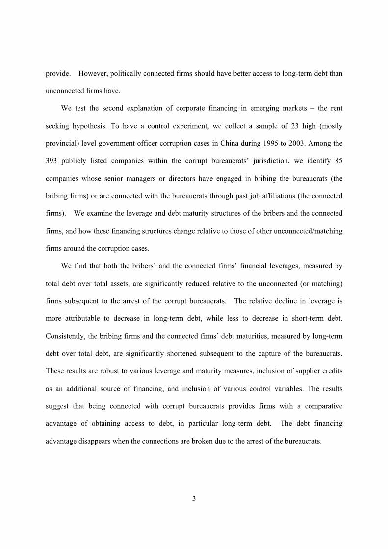
1. Introduction

It is well known that debt, in particular short-term debt, is the dominant external financing

source for companies in developing economies and emerging markets. The high corporate

financial leverage in emerging markets, and more generally differences in corporate financing

structures across countries, can only be partially explained by conventional theories that focus on

firm or industry factors.1 More recent cross-country studies reveal that a significant part of the

corporate financing patterns unexplained by firm or industry factors can instead be explained by

country-level institutional factors (Demirguc-Kunt and Maksimovic, 1996, 1998, 1999, 2001;

Rajan and Zingales, 1995; Booth, Aivazian, Demirguc-Kunt, and Maksimovic, 2001; Giannetti,

2003; Fan, Titman, and Twite, 2005).

This study examines the impact of political rent seeking and corruption on corporate

financing decisions. In an economy plagued by corruption, firms are likely to finance with

more debt as opposed to equity. This may be the case for two reasons. First, debt provides a

higher degree of monitoring ability and enforcement by investors (Smith and Warner, 1979) than

an open-ended equity claim which provides little protection from expropriation by managers or

bureaucrats. Second, it may be easier for a corrupt bureaucrat to channel funds in the form of

loans to his connected firms through a bank he controls (La Porta et al., 2002; Sapienza, 2004),

rather than through the equity market that he has smaller ability to influence. Similar

considerations apply to debt maturity. Firms in a more corrupt system are more likely to use

short-term debts, because they provide better investor protection than long-term debts can

1 This literature includes Modigliani and Miller (1958), Miller (1977), Bradley, Jarrell, and Kim (1984); Myers and Majluf (1984), Titman and Wessels (1988), Barclay and Smith (1995), MacKay and Phillips (2001), and many others.

3

provide. However, politically connected firms should have better access to long-term debt than

unconnected firms have.

We test the second explanation of corporate financing in emerging markets – the rent

seeking hypothesis. To have a control experiment, we collect a sample of 23 high (mostly

provincial) level government officer corruption cases in China during 1995 to 2003. Among the

393 publicly listed companies within the corrupt bureaucrats’ jurisdiction, we identify 85

companies whose senior managers or directors have engaged in bribing the bureaucrats (the

bribing firms) or are connected with the bureaucrats through past job affiliations (the connected

firms). We examine the leverage and debt maturity structures of the bribers and the connected

firms, and how these financing structures change relative to those of other unconnected/matching

firms around the corruption cases.

We find that both the bribers’ and the connected firms’ financial leverages, measured by

total debt over total assets, are significantly reduced relative to the unconnected (or matching)

firms subsequent to the arrest of the corrupt bureaucrats. The relative decline in leverage is

more attributable to decrease in long-term debt, while less to decrease in short-term debt.

Consistently, the bribing firms and the connected firms’ debt maturities, measured by long-term

debt over total debt, are significantly shortened subsequent to the capture of the bureaucrats.

These results are robust to various leverage and maturity measures, inclusion of supplier credits

as an additional source of financing, and inclusion of various control variables. The results

suggest that being connected with corrupt bureaucrats provides firms with a comparative

advantage of obtaining access to debt, in particular long-term debt. The debt financing

advantage disappears when the connections are broken due to the arrest of the bureaucrats.

4

To examine whether any of the lost financing advantage is reflected in lower firm value, we

perform an event study in which we estimate the cumulative abnormal stock returns (CARs) of

the firms around the initial public release of the corruption news. We find that CARs, measured

within various event windows of different length, are positively related to change in leverage

around the corruption events. The event study results suggest that the stock markets discount

the value of the firms whose financial leverages reduce (or do not increase as much as other

firms) around the corruption events. In retrospect, bribing or being connected with bureaucrats

has gained firms debt financing advantages, before the bureaucrats are caught guilty. In

addition to the event study that focuses on short-term performance, we also examine the

associations between time-serial changes in financial policy and long-term performance of the

sample firms. To better isolate any short-term impacts of the corruption scandals and hence

further mitigating potential endogeneity, we examine changes in financing/performance

measures over a seven-year window centered by the corruption events, and find consistent

positive relations between the firms’ financing capacity and performance.

Finally, we attempt to address the question of whether the rent seeking activities and the

capital allocation efficiency of China’s financial system can co-exist, in that more efficient firms

are more likely to pay bribes or build connections to secure their access to capital. We are

unable to find such evidence.

The overall empirical evidence suggests that public sector governance affects corporate

financing behaviors. It corroborates previous cross-country studies pointing to the importance of

country institutional factors in shaping corporate financing decisions. In particular,

Demirguc-Kunt and Maksimovic (1999) report that companies in countries with higher quality

legal systems and property rights enforcement have longer debt maturity. Fan, Titman, and

5

Twite (2005) report that corporate capital structure and debt maturity decisions are closely

related to a country’s tax system, legal system, and corruption level.

This study is built on an economic literature showing that rent seeking importantly explains

firm behaviors and economic growth (Shleifer and Vishny, 1994, 1998; and many others).

Several recent papers report that a significant part of firm value comes from corruption and rent

seeking activities (Fisman, 2001; Johnson and Mitton, 2003; Ramalho, 2003). Faccio (2006)

shows cross-country evidence that firms seek rents from the state. Our finding that the rent

seeking factor influences the allocation of financial capital among firms is consistent with two

recent studies of the Chinese financial system suggesting that China’s institutional and regulatory

environments foster connection-based corporate governance (Allen, Qian, and Qian, 2005a, b).

Our evidence corroborates with Johnson, McMillan, and Woodruff (2002) and Acemoglu

and Johnson (2005) showing that the risk of expropriation by governments is a fundamental

factor that shapes the financial development of a country. Durnev, Li, Morck, and Yeung (2004)

show that the low efficiency of some transition economies’ capital markets in disseminating

firm-specific information is closely related to weak property rights protection and poor

government quality. Our study complements several studies that examine the roles of political

connectedness in corporate financing behaviors. Charumilind, Kali, and Wiwattanakantang

(forthcoming) find that Thai-firms with connections to banks and politicians have more

long-term debt than firms without such ties do. Leuz and Oberholzer-Gee (2005) report that

politically connected firms in Indonesia are less likely than politically unconnected firms to raise

equity capital in foreign markets, possibly because domestic banks provide the connected firms

with capital at low costs. Cull and Xu (2005) report that access to bank loans is associated with

more firm investment in China, and that the Chinese firms’ investment behaviors are related to

6

both the risk of government expropriation and contract enforcement. Khwaja and Mian (2005)

report that politically connected firms in Pakistan receive abnormal lending from government

banks and suffer from abnormal default rates. Dinc (2005) in a cross-country study reports that

government owned banks tend to increase their lending in election years relative to private banks.

Siegel (2005) reports that Korean firms connected to politicians gain better access to key outside

resources through cross-border alliances. Faccio, Masulis, and McConnell (forthcoming) in a

cross-country study report that politically connected firms are more likely to be bailed out by

governments and their performance worsens more subsequent to their bailouts than

non-connected firms.

Compared with the prior studies, our single-country event study setting offers several

advantages. The empirical setting allows us to focus on a specific institutional factor, rent

seeking, while holding constant other institutional factors that might correlated with either rent

seeking or corporate financing decisions. Moreover, the empirical design addresses potential

endogeneity in the relations between corporate financing choices and corruption. Since the

connected firms are non-bribers, the corruption events are likely to be unexpected shocks. The

subsequent changes in their leverage and debt maturity structures are less likely caused by their

direct involvement in the corruption cases, but more likely due to lost connections with the

corrupt bureaucrats.

The remainder of the paper proceeds as follows. Section 2 provides an overview of China’s

financial markets and rent seeking activities. Section 3 presents the sample, data, and the

empirical results of the effects of the corruption events on capital and debt maturity structures.

Section 4 analyzes the roles of financial policy changes in performance. Section 5 addresses

the effects of corruption on capital allocation. Section 6 concludes the paper.

7

2. Institutional setting

This section describes China’s rent seeking and corruption activities, its financial markets,

and how the rent seeking activities shape firms’ financing decisions.

2.1. Corruption in China

China is rapidly becoming one of the largest economies in the world as well as a leading

destination for investments. However, it is also regarded as a highly corrupt country by world

standards. The Heritage Foundation and The Wall Street Journal co-publish the Index of

Economic Freedom, which ranks countries on 50 independent economic variables, including

ones relating to corruption in the judiciary, the rule of law, and the ability to enforce contracts.

Overall, the U.S. ranks the 6th, while China ranks the 128th out of 161 countries.2 La Porta,

Lopez-de-Silanes, Pop-Eleches and Shleifer (2004) find that China ranks among the worst

countries in terms of political freedom as well as the protection of property rights. China is

ranked 71 out of 145 based on the Corruption Perception Index of Transparency International.3

According to the official record of the Central Commission for Discipline Inspection of the

Communist Party of China during 1997-2002, there are totally 861,917 corruption cases under

investigation, 842,760 corruption cases concluded and 846,150 people punished by communist

laws, of which 137,711 expelled from the communist party.

2.2. Corporate financing activities in China

China has maintained a government dominated financial system. The government tightly

controls entry to commercial banking, investment banking and other financial services. The

banking system in China comprises the central bank, four large state-owned commercial banks,

2 More details are available at: http://cf.heritage.org/index/country.cfm?ID=30.0 3 The index measures the “degree to which corruption is perceived to exist among public officials and politicians. It is a composite index, drawing on 14 different polls and surveys from seven independent institutions, carried out among business people and country analysis, including surveys of residents, both local and expatriate.” Source: Transparency International.

8

three policy banks4, ten national joint-stock commercial banks, about 90 regional commercial

banks, and about 3,000 urban and 42,000 rural credit cooperatives. There are also branches or

representative offices of foreign banks with limited activities. Overall, the four state-owned

commercial banks dominate the market.5

Even though China’s two major stock exchanges—Shanghai and Shenzhen—have only

existed since 1990 and 1991, respectively, the number of companies listed on them have grown

to 1,377 by the end of 2004. The total market capitalization of these listed firms on that date was

US$448.6 billion, which was equal to about 36% of China’s gross domestic product.6 Despite

this phenomenal growth, equity financing still lagged far behind debt financing as the country’s

mode of financing for the period from 1993 to 2001.7

Allen, Qian and Qian (2005a, b) find that debt-financing is the dominant mode of corporate

finance and most bank credits are issued to companies in the State and Listed Sectors. They also

show that China’s banking system is run at low efficiency, as in the amount of non-performing

loans (NPL) within the four state commercial banks. 8 A large proportion of these

4 The three policy banks were established during the reform of the financial system in 1994 to take over the responsibilities of making policy loans from the four state commercial banks. Their mandates include making policy or low-interest loans to large government infrastructure investment projects specified by the government polices, providing agricultural financial services and subsidiary financing for the acquisition and storage of agricultural products, and supporting import and export credit for electronic and machinery equipment systems. 5 The four state-owned banks are Industrial and Commercial Bank of China (ICBC), the Agriculture Bank of China (ABC), Bank of China (BOC) and China Construction Bank (CCB). As of late 2001, they accounted for 63 percent of loans outstanding and 62 percent of deposits. With 103,000 branches among them, they are the only financial institutions that cover virtually all locations in China. 6 This information is obtained from the China Securities Regulatory Commission (CSRC) website: http://www.csrc.gov.cn. 7 The role of the equity markets in the Chinese economy is much less important than that of banks. Based on China Statistical Yearbook 2002, the accumulated capital raised from stock markets is RMB670 billion yuan (US$79 billion), while bond outstanding is RMB86 billion yuan (US$10 billion) and bank loans outstanding is RMB9,937 billion yuan (US$1,197 billion). The capital raised from stock issuance is only 6.5% of the capital raised from both bank loan and bond issuance. Tong (2005) estimates that equity financing only represented 10% to 20% of all financing for the listed firms in this period. 8 Statistics show that the outstanding NPL of major Chinese banks remained at 2.44 trillion yuan (289.96 billion US dollars) by the end of 2003, with an NPL ratio of 17.8 percent. The big four state-owned commercial banks accounted for 1.91 trillion yuan (230.76 billion US dollars), with an NPL of 20.36 percent.

9

non-performing loans are resulted from poor lending decisions made for state-owned enterprises,

some of which are due to political or other non-economic reasons.

As significant resources in transitional China are still allocated either directly or indirectly

by the state, politicians and bureaucrats are likely exert important influences on the allocation of

scarce resources such as bank loans. On the other hand, corruption is pervasive in the financial

sector of China.9 Obtaining large scale data on such detected or undetected criminal cases is

difficult, due to China’s opaque information disclosure. However, the review of the overall

financial system and stylized observations suggest that a link between corporate finance and rent

seeking is plausible. We proceed to examine such links in the next section.

3. Empirical analysis

This section describes the sample, provides basic statistics of the financing structures of the

sample firms, and reports regression results of the effects of rent seeking on the financing

structures of the firms around the corruption events.

3.1. The sample

To examine how corporate financing policies change with rent seeking activities, we

compile a list of corruption cases that involve high level government officers in China, and

identify listed companies that are connected to these corrupt bureaucrats.

We employ the following procedure to collect corruption cases. First, we identify a list of

corrupt bureaucrats, based on two government publications: Excerpts of Discipline Cases of the

9 Chinese anti-corruption officials have turned their sword to the financial industry recently, as the corruption in the financial system is viewed as more destructive to the country's financial health than other problems. Wang Xuebing, former governor of the Construction Bank of China, was sentenced to 12 years imprisonment in 2002 on a charge of accepting bribes worth 1.15 million yuan (US$139,000) in 1993-2001. Liu Jinbao, vice president of the Bank of China, received suspended death sentence in 2005. Prosecutors accused Liu of embezzling 14.48 million yuan (US$1.75 million), of which he personally pocketed 7.72 million yuan. He also received bribes amounting to 1.43 million yuan and was unable to account for 14.78 million yuan in personal assets.

10

Communist Party of China and Villains of the Communist Party of China10. We also make efforts

to collect additional corruption cases publicized by the Central Commission for Discipline

Inspection of the Communist Party of China. Totally we are able to identify 23 high level

government officer corruption cases occurred from 1995 to 2003.

Among the 23 cases, 19 involve provincial level government bureaucrats, two involve

central government bureaucrats, and two cases involve top executives of major state-owned

national banks. For each of the provincial corruption cases, we examine all publicly traded

companies located in the corrupt bureaucrat’s jurisdiction around the corruption event. For

each of the companies, we search through the company’s initial public offering prospectus and

annual reports prior to the corruption event to find out whether any of the company’s senior

managers, directors, or top-10 shareholders have engaged in bribing the bureaucrat. This is

done by searching through the above government publications and news disclosures during

investigation and lawsuit. For the 4 remaining cases that involve the central government and

banks, we are able to identify publicly listed firms that have bribed these government/bank

officers. Totally we identify 43 companies as bribers.

To facilitate a natural experiment, we next turn to identify a set of firms that are connected

with the corrupt bureaucrats but are not bribers nor otherwise involved in the corruption cases.

Again, for each company located in the jurisdiction of a corrupt bureaucrat, we search through

the public disclosures to find out whether any senior managers, directors, or large shareholders

are family members of or have prior job affiliation with the corrupt bureaucrat. We are able to

identify 42 companies with such connections.11 We call them connected firms. Finally,

10 The book titles are translated from Chinese. 11 Almost all of them are job connections. Family ties are rare.

11

there are remaining 308 listed companies in the corrupt bureaucrats’ jurisdictions but are neither

bribers nor connected with the bureaucrats. We call them unconnected firms.

Below is an example of the search process. A criminal case was initially exposed in

Jiangshu province in 1994. It was reported that Wuxi Xing Xing Industrial Ltd. illegally took

substantial deposits (RMB 3.2 billion) from the public. During the investigation, it was found

that Li Ming (secretary of the Beijing’s mayor, Li Qiyan) was involved in the scandal. Li Ming

further professed corruption evidence of Zhou Beifang (chairman and CEO of Shougang Holding

HK Ltd.), Chen Jian (secretary of Chen Xitong, the secretary of the Communist Party of China in

Beijing), and Chen Xiaotong (son of Chen Xitong). In early 1995, Zhou Beifang, Chen Jian, and

Chen Xiaotong were arrested. On April 5, 1995, Wang Baosheng, vice mayor of Beijing,

committed suicide. Within the coming year, tens of Beijing officials were arrested. On July 31,

1998, Chen Xitong was finally sentenced to 16 years of imprisonment for corruption. Appendix

1 illustrates our classification of the bribers, the connected firms, and the unconnected firms in

the corruption case. There are totally 11 publicly traded companies in Beijing around the

corruption event. We are able to identify 5 bribers (one also have job connection), 3 connected

(but non-bribing) firms, and 3 unconnected firms.

Table 1 provides a description of the 23 corruption cases. The corruption cases are

initially disclosed (event day) during 1995 to 2003. The sentence day is usually a few months

to a few years subsequent to the event day. The punishment received by the arrested bureaucrats

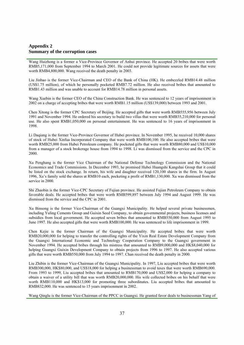
varies from death penalty to dismissal from position and/or the Communist Party. Appendix 2

provides a brief description of each of the corruption scandals. Many of the scandals involve

high-level bureaucrats receiving bribes in exchange of business opportunities or access to

financial capital (bank loans or stock listing status).

12

As in Table 1, the 393 firms in our sample (comprising the 43 bribing firms, the 42

connected firms, and the remaining 308 unconnected firms) do not concentrate in just a few

provinces but spread across the different China’s regions.

***************** Table 1 here

****************** For each of the 393 firms, we collect financial data up to 2004 from the China Stock Market

and Accounting Research (CSMAR) financial statement database.12 Daily stock prices are

obtained from the CSMAR transaction database. Twenty of the 393 firms do not have

pre-event financial data, of which 7 are bribing firms, 2 are connected firms, and 11 are

non-event firms. Hence the usable number of firms in our subsequent analysis is 373.

3.2. Sub-sample groupings

Our following analysis examines changes in capital structures of the bribing firms and the

connected firms around the corruption events, and compares the changes with those of the

unconnected firms. To facilitate discussion, we call the bribing firms and the connected firms

as “the event firms”, and the unconnected firms as “the non-event firms.” Separately, we

compare the financing patterns of the connected firms with those of the unconnected firms. As

discussed in the introduction, we are particularly interested in examining the financing patterns

of the connected firms around the corruption events, because the events are likely unexpected to

these firms. Any reaction of financing behaviors of the connected firms is therefore likely to be

caused by lost connections rather than by their involvement in the corruption.

As an alternative benchmark for comparison, we identify for each of the 373 usable sample

firms three matching firms that are closest to the matched sample firm in size (within the range

12 This database is developed by The Hong Kong Polytechnic University and Shenzhen GTA Information Technology Co. Ltd. It follows the format of CRSP and COMPUSTAT, and is the most comprehensive financial database available for listed Chinese firms.

13

from 0.5 to 1.5 times of the size of the sample firm), but located in different provinces from the

sample firm. Firm size is measured as the book value of assets at the year end prior to the arrest

of the corrupt bureaucrat. For each financial ratio of the sample firm, we match it with the

average ratio of the three matching firms.

3.3. Descriptive statistics

A few alternative measures of corporate financing structures are employed in this study.

Financial leverage is measured as total debt divided by total assets, or total debt plus accounts

payable divided by total assets. Debt maturity is measured as long-term debt divided by total

debt, or long-term debt divided by total debt plus accounts payable. We further define

long-term leverage as long-term debt divided by total assets, and short-term leverage as

short-term debt divided by total assets or short-term debt plus accounts payable divided by total

assets. The inclusion of accounts payable in the alternative leverage and debt maturity measures

is to account for supplier credits as a possible source of financing.13

Table 2 provides the basic statistics of the financing variables and other firm characteristics.

In Panels A and B respectively, we report the pooled firm-year mean and median values of each

of the variables during the three pre-event years, and over time change in the variable, defined as

the post-event three-year mean value of the variable minus the pre-event three-year mean value.

The event year is excluded from the analysis.14 Overall, these basic statistics suggest that the

event firms’ levels of assets, sales, and profitability do not change significantly over time.

However, the event firms seem to experience slower growth in assets and sales than that of the

13 Demirguc-Kunt and Maksimovic (2001) find that trade credit is an important source of financing in economies with underdeveloped financial intermediaries. 14 Results would not change if we include the event year observations in our analyses. For those firms with less than three year data either prior to or after the corruption events, we take the average of the available years before measuring change in a variable. However, the overall results in this paper would not change if we alternatively include only those firms with complete seven years of financial data.

14

non-event firms after the corruption events. In our subsequent regression analysis, we control

for the possibility that changes in the financing behaviors of the events firms around the

corruption events are due to changes in fundamentals, not just broken political connections.

***************** Table 2 here

****************** We have the following observations on changes in each of the financing variables for the

three sub-samples. First, firms in all of the three sub-samples experience rises in their financial

leverages over time, with the biggest increase taking place for the non-event firms. Second, the

mean debt maturity declines, and the magnitude of which is greater for the event firms than for

the non-event firms. Third, the mean long-term debt to assets ratio almost does not change

among the event firms, but it increases by about 4.2 percent among non-event firms. Fourth,

the mean short-term debt to assets ratio increases for both the event and non-event firms.

Lastly, the above observations hold true for the connected-firms-only sub-sample. From these

statistics, the corruption events seem to have larger effects on the event firms’ long-term

leverage than their short-term leverage.

It is interesting that the overall reported patterns are not only found in the bribing firms but

also in the connected firms that are non-bribers and are not directly involved in the corruption

cases. The changes in financing patterns of the connected firms are likely due to lost

connections with the arrested bureaucrats rather than due to the corruption events per se. This

implication motivates us to separately examine this connected-firms-only sub-sample in the

subsequent analysis.

3.4. Univariate analysis of net changes in capital structures

We next examine changes in financing structures of the event firms subsequent to the

corruption events, net of the corresponding changes of the non-event firms. We define the net

15

change in a financing variable as the difference in the change of the financing variable between

the event firms (as well as the connected firms) and the non-event firms. The change in the

financing variable of a firm is calculated as the three-year mean variable value after the

corruption event minus the three-year mean value before the event.

***************** Table 3 here

****************** Reported in Columns 2 and 3 of Panel A of Table 3, both the mean and median net changes

in the leverage ratios of the event firms are negative and statistically significant (at the 1 percent

level). These suggest that the event firms experience significant slower increase in debt

financing than the non-event firms do. The mean and median net changes in the debt maturity

ratios are negative, but are insignificant unless trade credits are considered. The net changes in

the long-term debt to assets ratio are negative and highly significant, suggesting a decline in

long-term financing of the event firms relative to that of the non-event firms. The net changes

in the short-term leverage ratios are also negative and significant. When we focus on the

connected firms only, we obtain the similar results (Columns 4 and 5).

Panel B of Table 3 employs the matching firms as an alternative benchmark for comparison

of changes in the event firms’ financing patterns. The results of the comparison with the

matching firms are weaker but consistent with those with the non-event firms in Panel A.

Overall, the significant differences in financing patterns between the event firms and their two

different sets of control firms suggest that the event firms are reasonably identified.

The above univariate results can be illustrated graphically. Figure 1 shows the patterns of

the annual mean debt to assets ratio from three years before to three years after the corruption

events. There is an overall increasing pattern of the mean leverage ratios. However, the mean

leverage ratio of the event firms is substantially slowed down around the corruption events and is

16

eventually lower than that of the non-event firms (Figure 1.1). The reversal in the leverage

ratio holds true even after excluding the bribing firms (Figure 1.2). Figure 2 plots the annual

mean long-term debt to total debt ratio for the event firms, the non-event firms, and the

connected firms. Overall the mean debt maturity ratios decrease. However, the event firms

experience more substantial drops in debt maturity relative to the non-event firms, and their debt

maturities become shorter than the non-event firms after the corruption events (Figure 2.1).

Similar results are found for the sub-sample of connected firms (Figure 2.2). Figure 3 plots the

patterns of the mean long-term debt to assets ratio. It shows a sharp decline in the long-term

leverage of the event firms around the corruption events (Figure 3.1). By contrast, the long-term

leverage of the non-event firms continues to increase through the event period. Excluding the

bribing firms, the long-term leverage of the connected firms still decreases around and after the

events (Figure 3.2).15

******************** Figures 1, 2, and 3 here

******************** 3.5. Regression analysis

We next perform regression analysis to examine whether the event firms’ financing policies

evolve after the corruption events in the predicted manners, controlling for other factors that are

known to affect leverage and debt maturity structures. The following regression models are

employed:

Financingit = α0i +α1Corruptit +α2Postit +α3Corruptit*Postit +α4Lassit +α5Tangibleit +α6Growthit +α7Profitit + industry dummy variables + εit

, where Financing represents a host of leverage and debt maturity variables measured in the

various ways defined previously; Corrupt is a dummy variable equal one if the firm is an event

15 Similar graphs are obtained using median values, or using matching firms as an alternative benchmark.

17

firm, and otherwise zero; Post is a dummy variable equal one if the observation is after the year

of the corruption event, and otherwise zero; Lass is the natural logarithm of total assets; Tangible

is fixed assets over total assets; Growth is market value of equity over book value of equity; and

Profit is net income over total assets. The regressions also include industry dummy variables.

Consistent with the literature, the inclusion of the assets, growth, and profitability variables is to

account for the possibility that some cross-sectional differences and/or over-time changes in

corporate financial policy are induced by differences/changes in corporate fundamentals.

3.5.1. The Event firms

We run a set of mean regressions including the pre- and post-event three-year mean values

of the dependent and independent variables as observations.16 The regressions employ 746

firm-period (373 firms time 2 periods) observations. We lose a few observations in some

regressions when firms have missing data on accounts payable or their debt maturity can not be

defined because of zero total debt. Panel A of Table 4 reports the results of mean leverage and

debt maturity regressions. We initially focus on Columns 2, 3, 4, and 5. The estimated

coefficients of the event firm dummy (Corrupt) are positive and significant in the leverage

regressions, indicating that the bribing firms and the connected firms have higher leverage. The

coefficient of Post is significantly positive in the leverage regressions (Columns 2 and 3) while

significantly negative in debt maturity regressions (Columns 4 and 5), consistent with the earlier

univariate results that financial leverage increases while debt maturity decreases over time.

We are particularly interested in the coefficient of the interaction term, Corrupt*Post. It is

negative and highly significant in each of the regressions, strongly suggesting that the event

16 Extreme values of the dependent and independent variables are winsorized. We also use median values in the regressions instead of means, results are similar.

18

firms’ leverage and debt maturity levels are substantially dampened upon and after the

corruption events.

We next turn to the long- and short-term leverage regressions (Columns 6-8). The

coefficient of Corrupt is insignificant for long-term leverage, indicating similar levels of

long-term leverage between the event firms and the non-event firms. The coefficient of Corrupt

is positive and significant at the 10-percent level for short-term leverage, implying the event

firms have marginally higher short-term leverage than the non-event firms. The coefficient of

Post is positive and significant throughout, suggesting overall increases in both short- and

long-term debt. The coefficient of the interaction term, Corrupt*Post, is negative and highly

significant in both the long-term and short-term leverage regression, suggesting that the event

firms’ long-term and short-term financing abilities are both weakened upon and after the

corruption events. However, the estimated coefficient of the interaction term in the long-term

debt ratio regression is significantly negative, suggesting an overall shortening of debt maturity.

The above changes in financing pattern around the corruption events cannot be explained

away by differences/changes in other corporate fundamentals, because these factors are

controlled in the regressions. However, some of these factors indeed affect the firms’ financing

patterns. Firm size (log assets) has strong positive effects on leverage and debt maturity.

Asset tangibility has a positive effect on leverage and debt maturity. Specifically, it has a

positive effect on long-term debt but a negative effect on short-term debt and trade credits. It

indicates that firms with few tangible assets tend to rely more on short-term financing while less

on long-term financing. The effects of sales growth are largely significant and positive on

leverage but insignificant for debt maturity. Profit has a negative effect on leverage, but its

19

effects on debt maturity are insignificant. These relations are largely consistent with those

reported in the prior literature.

Overall, the results in Panel A of Table 4 are consistent with that the event firms indeed

enjoy an advantage in raising debt capital compared with the non-event firms; but the advantage

discontinues when their political connections disappear with the arrest of the corrupt bureaucrats.

***************** Table 4 here

****************** Panel B of Table 4 provides mean regression results similar to Panel A, except that the

non-event firm observations are replaced by the matching firm observations. Here the dummy

variable Corrupt is equal to one if an observation is from an event firm, and zero if the

observation is otherwise from a set of matching firms. The results of the mean regressions

remain similar but weaker. In particular, the coefficient of the interaction term, Corrupt*Post,

is negative but insignificant in the leverage ratio regressions (Columns 2 and 3). The

coefficient is still negative and significant in the debt maturity and long-term leverage

regressions. The estimated coefficients of the control variables are similar to those reported in

Panel A.

As a robustness check, we also run the regressions on a pooled sample of event and

non-event firms covering firm-year observations from three years before to three years after the

corruption events, excluding the event year. Since the residual of a given firm may be correlated

across years for a given firm and the residuals of a given year may be correlated across firms, we

estimate our coefficients using clustered standard errors as Peterson (2005) to account for the

dependence in the residuals. We obtain similar results as those in the mean regressions.

Therefore we do not tabulate these results.

20

3.5.2. The connected firms

It could be the case that the above results are mostly attributable to the bribing firms. It

would be more useful to know whether the deteriorated financing advantage associated with the

corruption events can also be explained by lost political connection alone. For that reason we

repeat the regression analysis on the connected firms only.

Panel A of Table 5 reports mean regression results based on the combined sample of the

connected firms and the non-event firms. The dummy variable Corrupt is defined as one if the

firm is a connected firm, and zero otherwise. We find that the estimated coefficient of the

interaction term, Corrupt*Post, is negative but insignificant in the leverage regressions (Columns

2 and 3). The coefficient of the interaction term is negative and significant in the debt maturity

and the long-term leverage regressions (Columns 4, 5, and 6).

***************** Table 5 here

****************** We repeat the regressions based on the combined sample of the connected firms and their

matching firms. Panel B of Table 5 reports the regression results. The dummy variable

Corrupt is equal to one if the observation is from a connected firm, and zero if it is from a set of

matching firms. The results based on the matching firm benchmark are similar. Again, the

regression results show significant negative effects of the corruption events on the connected

firms’ debt maturity and long-term leverage, as revealed in the negative coefficients of the

interaction term, Corrupt*Post, in Columns 4, 5 and 6. The coefficients of the leverage ratios

are insignificant (Columns 2 and 3).

We alternatively perform pooled regressions with the clustered standard error adjustment.

The results (not reported) are consistent with those in Table 5.

21

The overall evidence in Tables 4 and 5 suggest that the debt financing capacity of the event

firms is substantially weakened after the corruption events, particularly so for their long-term

debt financing strength. The results hold even if we exclude the bribing firms, suggesting that

the weakened debt financing pattern is not just caused by the corruption cases but also related to

the lost political connections with the corrupt bureaucrats.

3.5.3. The non-event firms

We next examine the financing patterns of the non-event firms – the firms in the corrupt

bureaucrats’ jurisdiction but are not involved in the corruptions nor connected with the

bureaucrats. Because the non-event firms are also headquartered in the same province as the

corrupt bureaucrats, their financing behaviors may be impacted. We repeat the regression

analysis on the non-event firms and their matching firms. We redefine Corrupt as one (perhaps

unreasonably) when an observation is from a non-event firm, and zero if it is otherwise from a

set of matching firms.

The results of the mean regressions are reported in Table 6. We pay attention to the

coefficients of the interaction term, Corrupt*Post. Interestingly, they are positive and

significant in the leverage regressions, suggesting that the non-event firms’ debt ratios increase

relative to the matching firms after the corruption events. The increases are attributable to

increases in both long- and short-term debt, as indicated by the significant positive coefficients

of Corrupt*Post in the long- and short-term leverage regressions. There is no significant

difference in debt maturity between the non-event firms and their matching firms after the events.

These results suggest that, unlike the event firms which show weakened financing strength, the

non-event firms’ financing capacities show marginal improvement subsequent to the corruption

22

cases. The different results in the non-event firm sample also indicate that our classification

between the event firms and the non-event firms is reasonable.

***************** Table 6 here

******************

4. Capital structure changes and performance

We have established the relations consistent with the effects of rent seeking on capital

structures. The bribing firms and the connected firms have more debt and in particular long-term

debt in their capital structures, before the arrest of their connected bureaucrats. We next address

whether the changes in firm financial policies are associated with performance changes. In

Section 4.1., we conduct an event study to examine how stock markets react to the corruption

events, and whether stock prices incorporate the information of the leverage changes around the

events. In Section 4.2., we examine long-term changes in accounting and stock-based

performance measures, and whether these performance changes can be related to changes in firm

capital structures.

4.1. The event study

To examine whether any of the lost financing advantages is reflected by lower stock

valuation, we perform an event study in which we estimate the cumulative abnormal stock

returns of the firms around the initial public release of the corruption news. The event day of a

corruption scandal is identified as the first day that the public is informed about the bureaucrat’s

wrongdoings. Such notices can be Shuang Gui (a government detention measure that orders the

person to confess his/her crimes at a specific location), arrestment, or removal from the current

position. The event days of the 23 corruption cases have been reported in Table 1.

23

The standard event study methodology is used to investigate how the corruption news

affects the stock prices of the firms. The abnormal return for security i on event date t is

)|( ,,, ttititi IRERAR −=

, where ARi,t, Ri,t, and )|( , tti IRE are the abnormal, actual, and expected returns for time period t,

respectively. It is the information on which the expected return depends. There are two

common ways for modeling the expected return: the mean adjusted returns model where It is a

constant, and the market model where It is the market return. We employ both methods in our

study. We use both equal- and value-weighted market returns when the market model is

employed. We accumulate ARi,t to obtain cumulative abnormal returns (CARs), using various

event windows ranging from 60 days before to 60 days after the event day. Because the results

are qualitatively similar, we report the results based on the market model and value-weighted

market returns.

Figure 4 shows the patterns of daily mean CARs around the corruption events.17 The

average CAR of the event firms is decreasing and lower than that of the non-event firms. The

mean CAR of the sample firms starts to decline since fifty days before the event day. It continues

to drop after the event day. The overall decrease during the event period (-60 to +60 day) is

rather small, about 2%. Most of the decline in mean CAR is attributable to the event firms. i.e.

the bribing and connected firms. The mean CAR of the event firms is negative 8% toward the

end of the event period. By contrast, the mean CAR of the non-event firms does not show a

significant downward trend. Overall, China’s stock markets seem to be able to differentiate

rent seekers from others.

17 Due to missing stock return data of some firms, the sample size is 391 firms.

24

****************** Figure 4 here

****************** To examine whether there is any association between changes in leverage and the stock

market reactions around the corruption events, in Table 7, we stratify the sample into three

terciles (bottom, middle, and top) based on the degree of change in the three-year mean debt to

assets ratio before and after the corruption events. We employ eight event windows of different

length, ranging from sixty days before to sixty days after the events. Overall, more positive

changes in leverage are associated with higher CARs, and more negative changes in leverage are

associated with lower CARs. When we compare the mean and median differences in CARs

between the top and the bottom terciles, we find that most of the mean and median CARs in the

top tercile are significantly higher than those in the bottom ones. Moreover, 33% of the firms

in the bottom tercile are either bribing firms or connected firms, while only 10% of the firms in

the top tercile are bribing or connected firms.

***************** Table 7 here

****************** We next perform regression analysis on the effects of firm financing changes on CARs.

The dependent variable is CAR, alternatively measured over the various event windows. The

key independent variable is change in leverage (Chglev), measured as the three-year mean

leverage after the event minus the three-year mean leverage before the event. We also include

the dummy variable, Corrupt, which is equal to one if a firm is an event firm, and otherwise zero.

All of the CAR regressions include the industry dummy variables.

The regression results in the left panel of Table 8 show that there is an overall significant

and positive association between CAR and change in leverage. This relation is statistically

significant in four of the eight event windows. From the estimated coefficients of Corrupt

25

which is negative and significant in most of the event windows, we learn that the event firms

tend to experience more negative stock market reactions than the non-event firms.

The right panel of Table 8 reports the results of the CAR regressions including an additional

interaction term, Chglev*Corrupt. This is to examine how the relation between CARs and

change in leverage differs between the event firms and the non-event firms. We find that the

coefficients of the interaction term are positive in most of the event windows, and significantly

so in four of the windows, indicating the event firms’ stock returns are more sensitive to the

changes in leverage than non-event firms around the corruption events. Given this, we still find

that the coefficients of Chglev are positive and significant in three of the event windows.

***************** Table 8 here

****************** In summary, we find that the stock markets in China understand that political connections

help firms to obtain debt capitals. During the corruption events, stock investors discount the

values of the firms when their financing advantages are lost along with their political

connections.

4.2. Long-term performance changes

The above event study results may still be subject to the short-term influences of the

corruption scandals. That is, the stock performance and the capital structure changes may both be

the short-term impacts of the scandals per se, hence their relations could be spurious. To

address this issue we examine long-term performance effects of the changes in the event firms’

financial policies. We focus on two performance measures: return on sales (ROS), and the

market-to-book ratio measured as the market value of common equity divided by book value of

common equity. To isolate the short-term influence of a corruption scandal, these performance

measures are estimated three-year before and three-year after the year when the scandal erupts.

26

We then estimate performance change of a firm by taking the difference between the post- and

pre-event performance measure of the firm. We also similarly estimate changes in firm

financial policies captured by the leverage ratio, the long-term leverage ratio, the short-term debt

ratio, and the maturity ratio as defined before.

Employing the full sample including the event and the non-event firms, we regress

performance change alternately on the change in the financing variables. We include the

Corrupt dummy as defined before, to control for unobserved differences between the event and

non-event firms that lead to performance change. In addition, to examine whether the event

firms’ performance has different sensitivity to financial policy changes, we include an interaction

term between the Corrupt dummy variable and each of the financial variables alternately. If by

our empirical design the event firms’ changes in the performance and financing measures are

free of the short-term impact of the scandals, their sensitivities between financing and

performance should be indifferent from those of the non-event firms. Therefore the estimated

coefficients of the interaction terms are expected to be insignificantly different from zero. The

regressions also include the industry dummy variables.

***************** Table 9 here

***************** Panel A of Table 9 reports the regression results. Generally, capital structure changes are

positively associated with performance changes, as indicated by the positive estimated

coefficients of the capital structure variables. In particular, a decrease in the long-term debt

ratio is associated with a significant decrease in ROS. Financing changes that lead to decreased

total debt, long-term debt, short-term debt, or debt maturity are all associated with significant

decrease in the market-to-book ratio. These results suggest that debt financing, in particular

long-term debt financing capacity is vital to the performance of the firms.

27

The coefficients of the Corrupt dummy variable are generally negative but significantly so

only in the ROS regressions. The coefficients of the interaction terms between Corrup and

alternately the financing variables are mostly insignificantly different from zero, suggesting

indifferent sensitivity of performance to financial policy changes between the event firms and the

non-event firms. This is as expected.

The above results may still be subject to the endogeneity issue that the bribing firms’

financing and performance are both punished even in the long-term and hence their relations are

spurious. To mitigate this issue, we remove the bribing firms, hence leaving the connected

firms and the non-event firms in the sample, and re-run the regressions. The results, as reported

in Panel B of Table 9, remain similar.

We re-run the regressions using different performance measures including return on equity,

return on assets, and operating income over sales. The results are robust to the different

performance measures. As a further robustness check, we re-define the performance and

financing variables as two-year averages and re-run the regressions. For each firm associated

with a corruption event, we estimate post- and pre-event differences in two-year average

performance/financing ratios. Each of the post- (pre-) event performance/financing ratios is

calculated as the average ratio of the second and third year after (before) the scandal. Using

these changes in two-year average ratios in the regressions yields similar results.

In summary, we have reported that the weakened financing capacity due to lost political

connections has negative impacts on firm value as suggested by the patterns of short-term stock

return. More generally, exogenous shocks (exposing corruption scandals) that change the relative

financing strength of firms have long-term impacts on firm performance.

28

Finally, we run a series of sensitivity analyses to check the robustness of our key results in

Tables 4 through 9. As described in Appendix 3, these key results are robust to alternative

definitions of event firms, different degrees of corruption punishment, survivorship bias,

alternative scaling factors of the financing variables, and different length of event windows.

5. Does rent seeking facilitate capital allocation?18

The empirical results thus far have shown that the Chinese companies’ access to financial

capital critically depends on their rent seeking capacities. However, we are interested in

knowing whether or not the rent seekers are also efficient firms who bribe or invest in

relationships because they are affordable.19 It could be the case that China’s capital allocation

system, though opaque, still manages to allocate financial capital to efficient firms. If so,

exposing corruption scandals has a side effect of punishing efficient firms. A different

possibility is that the rent seekers tend to be firms uncompetitive in terms of

managerial/production efficiency, but gain their competing edge through political connections or

outright bribery. In this scenario, the problem of China’s financial system is not just social

injustice but also mis-allocation of capital. Fighting corruption is unambiguously desirable

because it will punish bad firms and promote good firms.20 A third possibility is that given a

non-transparent capital allocation system, everyone pays bribe to stay in the game, and whoever

caught is a random event. In this scenario exposing scandals is expected risk with no

implication on economic outcome.

18 This section has benefited from the suggestions of Bernard Yeung. 19 Some argue that corruption can serve as grease to facilitate business transactions. This view has been expressed in business press as well as in the economic literature (Lui, 1985). 20 There exists a large amount of evidence that corruption slows down economic growth and domestic and foreign investment. See Bardhan (1997) and Aidt (2003) for an overview of the literature.

29

We are not able to examine the issue fully in this paper, as our sample and data are specific

to the few corruption cases. Nevertheless, we attempt to address the question by examining

several performance measures of the event firms (relative to the non-event firms) both well

(three-year) before and well (three-year) after their corresponding corruption cases erupt, so that

the performance measures are away from the direct influence of the corruption cases per se.

The performance measures capture the differences in profitability between the event and the

non-event firms.21 If the event firms behave more as rent seekers because they are more

efficient than the non-event firms are, we would observe their pre-event performance superior to

that of the non-event firms, and their post-event performance no worse than that of the non-event

firms. 22 However, if the event firms gain their competitive edge not from

managerial/productive efficiency but mostly from rent seeking, we would expect that removing

their political connections would lead to their poorer performance relative to the non-event firms.

If the randomness argument is true, that the event and non-event firms are both rent seekers and

their rent seeking activities have little to do with their managerial/production efficiency, then

there would be little difference in their performance prior to the events, but the non-event firms

would outperform the event firms after the events.

Table 10 presents differences in mean and median performance measures between the event

firms and the non-event firms. Performance is measured alternatively by return on assets (ROA),

return on equity (ROE), operating margin (operating income divided by sales), return on sales

(ROS), and the market to book ratio (market value of equity divided by book value of equity).

As in the previous section, these performance measures are calculated for each of the event and

21 The differences in profitability reflect the differences in both productivity and rent seeking capability between the event and the non-event firms. 22 We are assuming that the event and non-event firms are competing for an overlapping set of business opportunities, and that the scandals per se do not have long lasting impacts on firm productivity.

30

non-event firms at the fiscal year end of the third year before and the third year after the

corresponding corruption event year. From Panel A, the between-group performance

differences before the events are generally positive in mean or median, but insignificantly so

except for the market-to-book ratio. After the events, the performance differences are mostly

negative and statistically significant, except for the market-to-book ratio showing insignificantly

positive values. In Panel B, we remove the bribing firms and focus our comparison between the

connected firms and the non-event firms. We find that none of the measures show significant

difference in performance between the connected and the non-event firms prior to the scandals.

However, after the scandals the connected firms underperform the non-event firms, and

significantly so in terms of ROA, ROS, and operating margin.

****************** Table 10 here

****************** The statistics in Table 10 suggest that the event firms do not significantly outperform the

non-event firms before the corruption scandals are exposed, while they substantially

underperform the non-event firms subsequent to the scandals. The evidence is inconsistent with

the view that efficient firms pay bribes or build political connections to gain access to financial

capital. Rather, the evidence is more consistent with the second scenario that the event firms

gain their financing and possibly other competitive advantages primarily from rent seeking,

because their performance clearly become worse than the non-connected firms even long after

the scandals. However, we are unable to reject the third randomness view that rent seeking is

pervasive among both the event and non-event firms, as we do not have strong evidence that

their performance are different prior to the scandals.

Overall, we do not find evidence that financial capital is allocated to rent seekers because

they are efficient firms. By contrast, we find these firms become uncompetitive once their

31

political connections are removed as the corruption scandals are exposed. A reason why

corruption fails to grease but clogs business transactions is that government regulations are

endogenous to bureaucrats’ incentive to seek rents (Shelifer and Vishny, 1993, 1994). A

less-than-benevolent bureaucrat can create red tapes to expropriate business rents. Consistently,

Kaufmann and Wei (1998) report that corruption is not associated with decreased but with

increased business costs.

6. Conclusions

We have examined the impact of corruption and rent seeking on corporate financing

behaviors in China. This is done through an event study. We identify publicly listed firms

who engage in bribing or are connected with corrupt high level government bureaucrats. We

find that both the bribers’ and the connected firms’ financial leverages are significantly reduced

relative to their control firms subsequent to the arrest of the corrupt bureaucrats. The relative

declines in leverage are mainly due to decreases in long-term debt, while the relative levels of

short-term debt are less significantly changed. Consistently, the bribing firms and the

connected firms’ debt maturities are significantly shortened subsequent to the capture of the

bureaucrats. These results suggest that being connected with corrupt bureaucrats provide firms

with a comparative advantage of access to debt, in particular long-term debt. The debt

financing advantage disappears when the connections are broken due to the arrest of the

bureaucrats.

We have also examined whether any of the lost financing advantages is reflected in poor

firm performance. The prediction is confirmed in our study of stock return patterns around the

corruption events. The results suggest that the stock markets discount the values of the firms

32

whose financial leverages reduce (or do not increase as much as other firms) around the

corruption events. In addition, our analysis of long-term changes in firm financing policies and

performance, which excludes the short-term impact of the corruption scandals, finds that access

to financial capital is vital to firm competitiveness. Finally, we find little evidence from the

sample suggesting that rent seeking facilitates capital allocation in China.

Our study makes several contributions to the literature. First, it provides evidence of the

importance of institutional factors in shaping corporate financing choices, which is beginning to

draw researchers’ attention. Second, our single-country setting and the time-serial empirical

design provide more robust evidence, as it is less subject to endogeneity and omitted variable

problems that are common in cross-sectional studies. Third, the results of this paper help policy

makers to gauge the importance of fighting corruption and building market supporting

institutions. The evidence from China is useful to other emerging markets plagued by similar

institutional problems.

33

References:

Acemoglu, D., and Johnson, S., 2005, Unbundling Institutions, Journal of Political Economy 113, 949-995. Aidt, T.S., 2003, “Economic Analysis of Corruption: A Survey,” Economic Journal 113, 632-652. Allen, F., Qian, J., and Qian, M.J., 2005a, “Law, Finance, and Economic Growth in China”, Journal of Financial Economics, 77, 57-116. Allen, F., Qian, J., and Qian, M.J., 2005b, “China’s Financial System: Past, Present, and Future“, book chapter in The Transition that Worked: Origins, Mechanism, and Consequence of China’s Long Boom, edited by L. Brandt and T. Rawski. Barclay, M.J., and Smith, C.W., 1995, “The Maturity Structure of Corporate Debt”, Journal of Finance, 50, 609-631. Bardhan, P., 1997, “Corruption and Development: A Review of Issues,” Journal of Economic Literature 35, 1320-1346. Booth, L., Aivazian, V., Demirguc-Kunt, A., and Maksimovic, V., 2001, “Capital Structures in Developing Countries,” Journal of Finance, 56, 87-130. Bradley, M., Jarrell, G.A., and Kim, H., 1984, “On the Existence of an Optimal Capital Structure”, Journal of Finance, 39, 857-878. Charumilind, C., Kali, R., and Wiwattanakantang, Y., forthcoming, “Crony Lending: Thailand before the Financial Crisis,” Journal of Business. Cull, R., and Xu, L.C., 2005, “Institutions, Ownership, and Finance: The Determinants of Profit Reinvestment among Chinese Firms,” Journal of Financial Economics 77, 117-146. Demirguc-Kunt, A., and Maksimovic, V., 1996, “Stock Market Development and Firm Financing Choices”, World Bank Economic Review, 10, 341-369. Demirguc-Kunt, A., and Maksimovic, V., 1998, “Law, Finance and Firm Growth”, Journal of Finance, 53, 2107-2137. Demirguc-Kunt, A., and Maksimovic, V., 1999, “Institutions, Financial Markets, and Firm Debt Maturity,” Journal of Financial Economics 54, 295-336. Demirguc-Kunt, A., and Maksimovic, V., 2001, “Firms as Financial Intermediaries: Evidence from Trade Credit Data,” Working Paper, World Bank and the University of Maryland.

34

Dinc, I.S., 2005, “Politicians and Banks: Political Influences on Government-owned Banks in Emerging Markets,” Journal of Financial Economics 77, 453-479. Durnev, A., Li, K., Morck, R., and Yeung, B.Y., 2004, "Capital Markets and Capital Allocation: Implications for Economies in Transition," Economics of Transition 12, 593-634. Faccio, M., 2006, Politically Connected Firms, American Economic Review 96, 369-386. Faccio, M., Masulis, R., and McConnell, J.J., forthcoming, “Political Connections and Corporate Bailouts,” Journal of Finance. Fan, J.P.H., Titman, S., and Twite, G., 2005, “An International Comparison of Capital Structure and Debt Maturity Choices,” Working Paper, Chinese University of Hong Kong, University of Texas – Austin, and University of New South Wales. Fisman, R., 2001, “Estimating the Value of Political Connections,” American Economic Review, 91, 1095-1102. Giannetti, M., 2003, “Do Better Institutions Mitigate Agency Problems? Evidence from Corporate Finance Choices”, Journal of Financial and Quantitative Analysis, 38, 185-212. Johnson, S., McMillan, J., and Woodruff, C., 2002, “Property Rights and Finance,” American Economic Review, 92, 1335-1356. Johnson, S., and Mitton, T., 2003, “Cronyism and Capital Controls: Evidence from Malaysia,” Journal of Financial Economics, 67, 351-382. Kaufmann, D., and Wei, S.J., 1998, “Does “Grease Money” Speed Up the Wheels of Commerce?”, Working Paper, World Bank and Harvard University. Khawaja, A.L., and Mian, A., 2005, “Do Lenders Favor Politically Connected Firms? Rent Provision in An Emerging Financial Market,” Quarterly Journal of Economics 120, 1371-1411. La Porta, R., Lopez-de-Silanes, F., Shleifer, A., and Vishny, R., 2002, “Government Ownership of Banks,” Journal of Finance 57, 265-301. La Porta, R., Lopez-de-Silanes, F., Pop-Eleches, C., and Shleifer, A., 2004, “Judicial Checks and Balances,” Journal of Political Economy, 112, 445-470. Leuz, C., and Oberholzer-Gee, F., 2005, “Political Relationships, Global Financing, and Corporate Transparency,” Working Paper, Wharton School and Harvard Business School. Lui, F., 1985, “An Equilibrium Queuing Model of Bribery,” Journal of Political Economy 93, 760-781.

35

MacKay, P., and Phillips, G.M., 2001, “Is There an Optimal Industry Capital Structure?” Working Paper, University of Maryland. Miller, M.H., 1977, “Debt and Taxes,” Journal of Finance, 32, 261-275. Modigliani, F., and Miller, M.H., 1958, “The Cost of Capital, Corporate Finance, and the Theory of Investment,” American Economic Review, 48, 261-297. Myers, S., and Majluf, N., 1984, “Corporate Financing and Investment Decisions When Firms Have Information That Investors Do Not Have,” Journal of Financial Economics, 13, 187-221. Peterson, M., 2005, “Estimating Standard Errors in Financial Panel Data Sets: Comparing Approaches,” Working Paper, Northwestern University. Rajan, R., and Zingales, L., 1995, “What Do We Know about Capital Structure? Some Evidence from International Data,” Journal of Finance, 50, 1421-1460. Ramalho, R., 2003, “The Effects of An Anti-Corruption Campaign: Evidence from the 1992 Presidential Impeachment in Brazil,” Working Paper, MIT. Sapienza, P., 2004, “The Effects of Government Ownership on Bank Lending,” Journal of Financial Economics, 72, 357-384. Shleifer, A., and Vishny, R., 1993, “Corruption,” Quarterly Journal of Economics 108, 599-617. Shleifer, A., and Vishny, R., 1994, "Politicians and Firms," Quarterly Journal of Economics 109, 995-1025. Shleifer, A., and Vishny, R., 1998, The Grabbing Hand: Government Pathologies and their Cures, Cambridge, MA: Harvard University Press. Siegel, J., 2005, “Contingent Political Capital and International Alliances: Evidence from South Korea,” Working Paper, Harvard Business School. Smith, C., and Warner, J.B., 1979, “On Financial Contracting: An Analysis of Bond Covenants,” Journal of Financial Economics 7, 117-161. Titman, S., and Wessels, R., 1988, “The Determinants of Capital Structure Choice”, Journal of Finance, 43, 1-19. Tong, D.C. 2005. “Corporate Governance and Securities Regulations in Mainland China”, Seminar Paper, China Securities Regulatory Commission, presented at Chinese University of Hong Kong (May 5).

36

Appendix 1

A Corrupt Bureaucrat and His Allies

This table shows the relationships between listed companies headquartered in Beijing and Chen Xitong, the secretary of the Communist Party of China in Beijing. Chen was sentenced to 16 years of imprisonment for corruption in 1998.

Firm Name Listed Market

Connection Type Note

Beijing Development

HK Colleague & Briber

Gao Qiming (chairman) was an ex-secretary of Chen Xitong. Besides, there were other three officials from the Beijing government sat on the company’s board.

Shougang Concord Century

HK Briber Zhou Beifang, chairman and CEO of the controlling shareholder (Shougang Holding) of the company, was the conspirator and briber of Chen Xitong.

Shougang Concord

Technology

HK Briber Zhou Beifang, chairman and CEO of the controlling shareholder (Shougang Holding) of the company, was the conspirator and briber of Chen Xitong.

Shougang Concord

International

HK Briber Zhou Beifang (chairman and CEO) was the conspirator and briber of Chen Xitong.

Shougang Concord Grand

HK Briber Zhou Beifang (chairman and CEO) was the conspirator and briber of Chen Xitong.

HK Beiren Printing Shanghai

Colleague Zhang Peng (director) was the vice mayor of Beijing City.

Beijing Auto Shanghai Colleague Zhu Lining (director) was the vice president of Beijing Municipal Finance Bureau.

Beijing Urban-Rural

Shanghai Colleague Both its chairman and vice-chairman had working experiences in the Beijing government.

Beijing Tianqiao Shanghai unconnected firm Not applicable Beijing Tianlong Shanghai unconnected firm Not applicable

Wangfujing Store

Shanghai unconnected firm Not applicable

37

Appendix 2 Summary of the corruption cases

Wang Huizhong is a former a Vice-Province Governor of Anhui province. He accepted 20 bribes that were worth RMB5,171,000 from September 1994 to March 2001. He could not provide legitimate sources for assets that were worth RMB4,800,000. Wang received the death penalty in 2003. Liu Jinbao is the former Vice-Chairman and CEO of the Bank of China (HK). He embezzled RMB14.48 million (US$1.75 million), of which he personally pocketed RMB7.72 million. He also received bribes that amounted to RMB1.43 million and was unable to account for RMB14.78 million in personal assets. Wang Xuebin is the former CEO of the China Construction Bank. He was sentenced to 12 years of imprisonment in 2002 on a charge of accepting bribes that were worth RMB1.15 million (US$139,000) between 1993 and 2001. Chen Xitong is the former CPC Secretary of Beijing. He accepted gifts that were worth RMB555,956 between July 1991 and November 1994. He ordered his secretary to build two villas that were worth RMB35,210,000 for personal use. He also spent RMB1,050,000 on personal entertainment. He was sentenced to 16 years of imprisonment in 1998. Li Daqiang is the former Vice-Province Governor of Hubei province. In November 1995, he received 10,000 shares of stock of Hubei Xinfua Incorporated Company that were worth RMB100,100. He also accepted bribes that were worth RMB25,000 from Hubei Petroleum company. He pocketed gifts that were worth RMB80,000 and US$10,000 from a manager of a stock brokerage house from 1994 to 1998. Li was dismissed from the service and the CPC in 2000. Xu Penghang is the former Vice Chairman of the National Defense Technology Commission and the National Economics and Trade Commissions. In December 1993, he promised Hubei Huangshi Kangshai Group that it could be listed on the stock exchange. In return, his wife and daughter received 120,100 shares in the firm. In August 1996, Xu’s family sold the shares at RMB10 each, pocketing a profit of RMB1,130,000. Xu was dismissed from the service in 2000. Shi Zhaobin is the former Vice-CPC Secretary of Fujian province. He assisted Fujian Petroleum Company to obtain favorable deals. He accepted bribes that were worth RMB599,897 between July 1994 and August 1999. He was dismissed from the service and the CPC in 2001. Xu Binsong is the former Vice-Chairman of the Guangxi Municipality. He helped several private businessmen, including Yuling Cements Group and Guixin Seed Company, to obtain governmental projects, business licenses and subsidies from local government. He accepted seven bribes that amounted to RMB550,000 from August 1995 to June 1997. He also accepted gifts that were worth RMB100,000. He was sentenced to life imprisonment in 1999. Chen Kejie is the former Chairman of the Guangxi Municipality. He accepted bribes that were worth RMB20,000,000 for helping to transfer the controlling rights of the Yixin Real Estate Development Company from the Guangxi International Economic and Technology Cooperation Company to the Guangxi government in November 1994. He accepted bribes through his mistress that amounted to RMB9,000,000 and HK$8,040,000 for helping Guangxi Guixin Development Company to obtain projects from 1996 to 1997. He also accepted various gifts that were worth RMB550,000 from July 1994 to 1997. Chan received the death penalty in 2000. Liu Zhibin is the former Vice-Chairman of the Guangxi Municipality. In 1997, Liu accepted bribes that were worth RMB300,000, HK$80,000, and US$18,000 for helping a businessman to avoid taxes that were worth RMB690,000. From 1993 to 1999, Liu accepted bribes that amounted to RMB170,000 and US$2,000 for helping a company to obtain a waiver of a utility bill that was worth RMB20,000,000. His wife collected bribes on his behalf that were worth RMB110,000 and HK$13,000 for promoting three subordinates. Liu accepted bribes that amounted to RMB832,000. He was sentenced to 15 years imprisonment in 2002. Wang Qinglu is the former Vice-Chairman of the PPCC in Guangxi. He granted favor deals to businessman Yang of

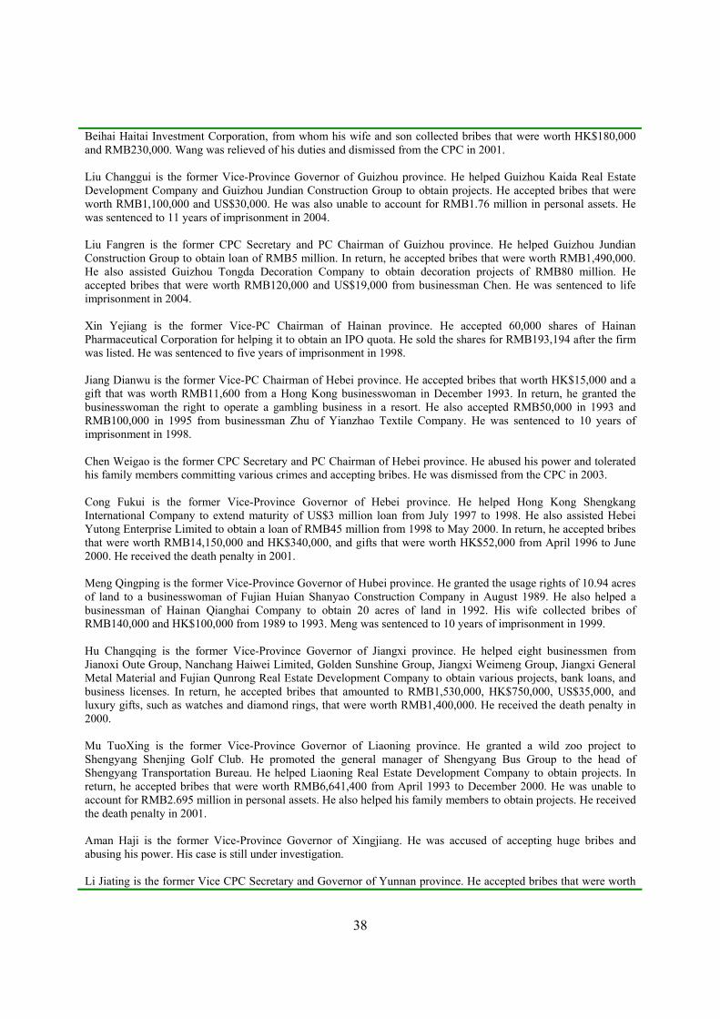
38

Beihai Haitai Investment Corporation, from whom his wife and son collected bribes that were worth HK$180,000 and RMB230,000. Wang was relieved of his duties and dismissed from the CPC in 2001. Liu Changgui is the former Vice-Province Governor of Guizhou province. He helped Guizhou Kaida Real Estate Development Company and Guizhou Jundian Construction Group to obtain projects. He accepted bribes that were worth RMB1,100,000 and US$30,000. He was also unable to account for RMB1.76 million in personal assets. He was sentenced to 11 years of imprisonment in 2004. Liu Fangren is the former CPC Secretary and PC Chairman of Guizhou province. He helped Guizhou Jundian Construction Group to obtain loan of RMB5 million. In return, he accepted bribes that were worth RMB1,490,000. He also assisted Guizhou Tongda Decoration Company to obtain decoration projects of RMB80 million. He accepted bribes that were worth RMB120,000 and US$19,000 from businessman Chen. He was sentenced to life imprisonment in 2004. Xin Yejiang is the former Vice-PC Chairman of Hainan province. He accepted 60,000 shares of Hainan Pharmaceutical Corporation for helping it to obtain an IPO quota. He sold the shares for RMB193,194 after the firm was listed. He was sentenced to five years of imprisonment in 1998. Jiang Dianwu is the former Vice-PC Chairman of Hebei province. He accepted bribes that worth HK$15,000 and a gift that was worth RMB11,600 from a Hong Kong businesswoman in December 1993. In return, he granted the businesswoman the right to operate a gambling business in a resort. He also accepted RMB50,000 in 1993 and RMB100,000 in 1995 from businessman Zhu of Yianzhao Textile Company. He was sentenced to 10 years of imprisonment in 1998. Chen Weigao is the former CPC Secretary and PC Chairman of Hebei province. He abused his power and tolerated his family members committing various crimes and accepting bribes. He was dismissed from the CPC in 2003. Cong Fukui is the former Vice-Province Governor of Hebei province. He helped Hong Kong Shengkang International Company to extend maturity of US$3 million loan from July 1997 to 1998. He also assisted Hebei Yutong Enterprise Limited to obtain a loan of RMB45 million from 1998 to May 2000. In return, he accepted bribes that were worth RMB14,150,000 and HK$340,000, and gifts that were worth HK$52,000 from April 1996 to June 2000. He received the death penalty in 2001. Meng Qingping is the former Vice-Province Governor of Hubei province. He granted the usage rights of 10.94 acres of land to a businesswoman of Fujian Huian Shanyao Construction Company in August 1989. He also helped a businessman of Hainan Qianghai Company to obtain 20 acres of land in 1992. His wife collected bribes of RMB140,000 and HK$100,000 from 1989 to 1993. Meng was sentenced to 10 years of imprisonment in 1999. Hu Changqing is the former Vice-Province Governor of Jiangxi province. He helped eight businessmen from Jianoxi Oute Group, Nanchang Haiwei Limited, Golden Sunshine Group, Jiangxi Weimeng Group, Jiangxi General Metal Material and Fujian Qunrong Real Estate Development Company to obtain various projects, bank loans, and business licenses. In return, he accepted bribes that amounted to RMB1,530,000, HK$750,000, US$35,000, and luxury gifts, such as watches and diamond rings, that were worth RMB1,400,000. He received the death penalty in 2000. Mu TuoXing is the former Vice-Province Governor of Liaoning province. He granted a wild zoo project to Shengyang Shenjing Golf Club. He promoted the general manager of Shengyang Bus Group to the head of Shengyang Transportation Bureau. He helped Liaoning Real Estate Development Company to obtain projects. In return, he accepted bribes that were worth RMB6,641,400 from April 1993 to December 2000. He was unable to account for RMB2.695 million in personal assets. He also helped his family members to obtain projects. He received the death penalty in 2001. Aman Haji is the former Vice-Province Governor of Xingjiang. He was accused of accepting huge bribes and abusing his power. His case is still under investigation. Li Jiating is the former Vice CPC Secretary and Governor of Yunnan province. He accepted bribes that were worth

39

RMB11,000,000 from 1994 to July 2000. He received the death penalty in 2003. Xu Yunhong is the former Vice-Province Governor of Zhejiang province. He helped Ningbao International Trust and Investment Corporation to obtain loans. He also committed malfeasance and caused huge losses of government assets worth RMB1.2 billion. He forced Ningbao Daily to purchase Huahong International Center building from a private owner businessman Zhong. It caused a huge economic loss for Ningbao Daily. In return, his son accepted bribes that were worth RMB5,690,000, HK$120,000, US$25,000, and a villa that was worth RMB850,000. He was sentenced to 10 years of imprisonment in 2000.

40

Appendix 3

Additional Robustness Tests

We run battery of sensitivity analyses to check the robustness of our key results. First, we

redefine our event firms. If a firm is identified as a briber or a connected firm in a corruption

case, the firm is classified as an event firm in every other corruption case occurred in the same

province. Previously, it is classified as an event firm only in the corruption case that it is

involved. The new definition gives us 102 event firms, of which 51 are connected firms. Our

analyses based on the new definition give qualitatively similar results.

We next examine whether different degrees of punishment in the corruption cases would

affect the event firms’ financing behaviors differently. We include those cases in which

bureaucrats are sent to prison or death role, while exclude those cases ended up with less serious

punishment such as expel from service or party. Our overall results remain similar.

Firms may be delisted from trading and hence creating survivorship bias in our analysis.

We find only five firms are delisted 1 year or 2 years after the events. Among the five firms, two

firms are event firms, while the other three are non-event firms. The small number of the delisted

firms has not caused systematic bias in our analysis.

To check if our results are sensitive to the choice of scaling factor, we use total sales as an

alternative scaling factor. The results remain intact. We also perform regression analysis on the

percentage changes in the level of total debt, long-term debt and short-term debt. Similar results

are obtained.

We also choose different event windows to examine the changes in firms’ financing. We

rerun the financing regressions (Tables 4-6) using paired data of year -1 with year +1, year -2

with year +2, or year -3 with year +3. Again, the results are similar and consistent.

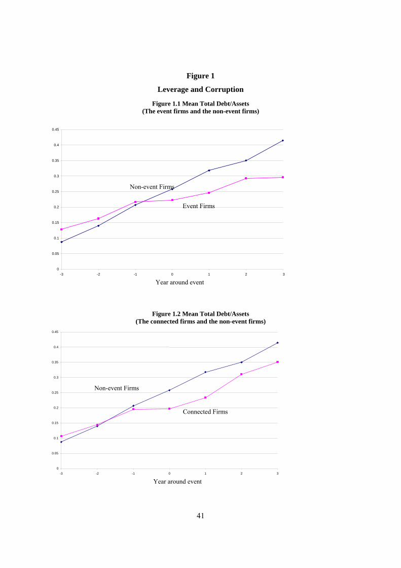
41

Figure 1

Leverage and Corruption

Figure 1.1 Mean Total Debt/Assets (The event firms and the non-event firms)

Figure 1.2 Mean Total Debt/Assets

(The connected firms and the non-event firms)

0

0.05

0.1

0.15

0.2

0.25

0.3

0.35

0.4

0.45

-3 -2 -1 0 1 2 3 Year around event

Event Firms

Non-event Firms

0

0.05

0.1

0.15

0.2

0.25

0.3

0.35

0.4

0.45

-3 -2 -1 0 1 2 3

Year around event

Connected Firms

Non-event Firms

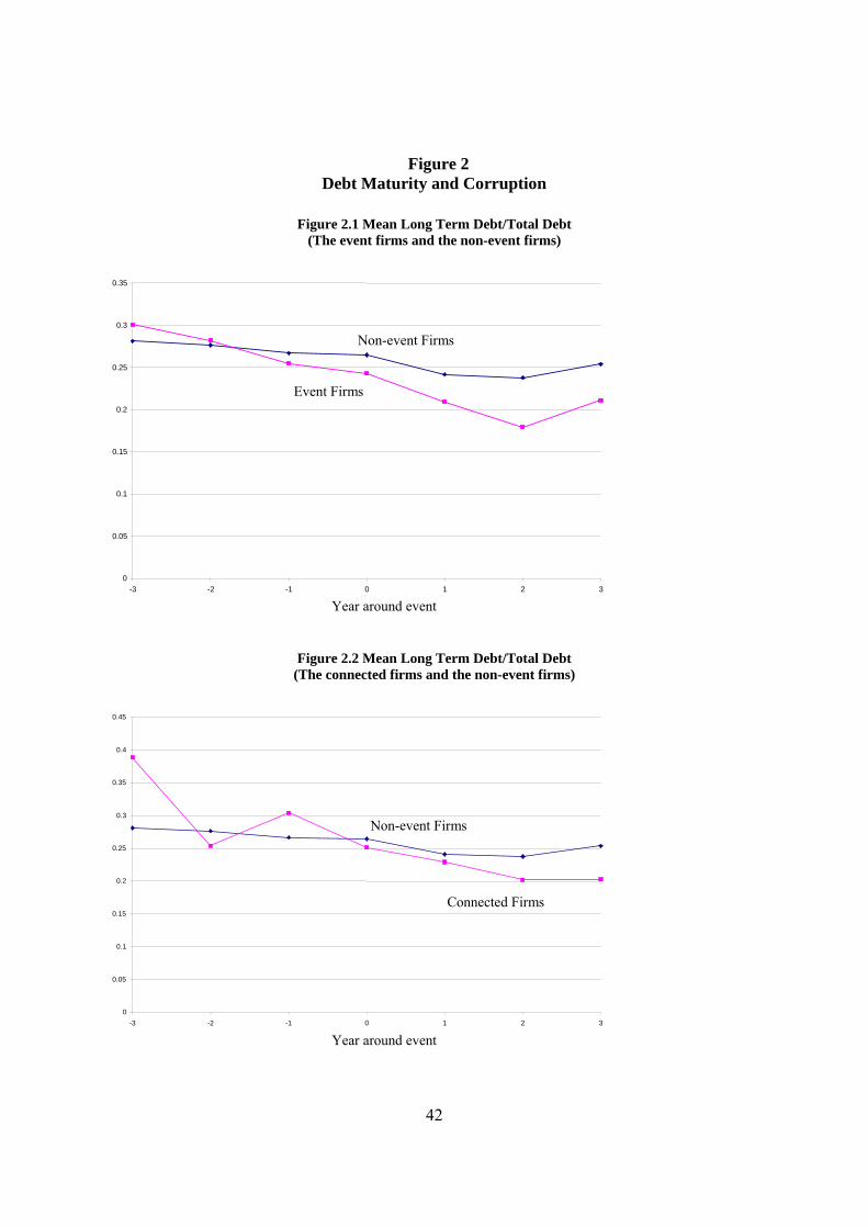
42

Figure 2 Debt Maturity and Corruption

Figure 2.1 Mean Long Term Debt/Total Debt

(The event firms and the non-event firms)

Figure 2.2 Mean Long Term Debt/Total Debt (The connected firms and the non-event firms)

0

0.05

0.1

0.15

0.2

0.25

0.3

0.35

-3 -2 -1 0 1 2 3

Year around event

Event Firms

Non-event Firms

0

0.05

0.1

0.15

0.2

0.25

0.3

0.35

0.4

0.45

-3 -2 -1 0 1 2 3

Year around event

Connected Firms

Non-event Firms

43

Figure 3 Long-term leverage and Corruption

Figure 3.1 Mean Long Term Debt/Assets (The event firms and the non-event firms)

Figure 3.2 Mean Long Term Debt/Assets (The connected firms and the non-event firms)

0

0.02

0.04

0.06

0.08

0.1

0.12

-3 -2 -1 0 1 2 3

Year around event

Event Firms

Non-event Firms

0

0.02

0.04

0.06

0.08

0.1

0.12

-3 -2 -1 0 1 2 3

Year around event

Connected Firms

Non-event Firms

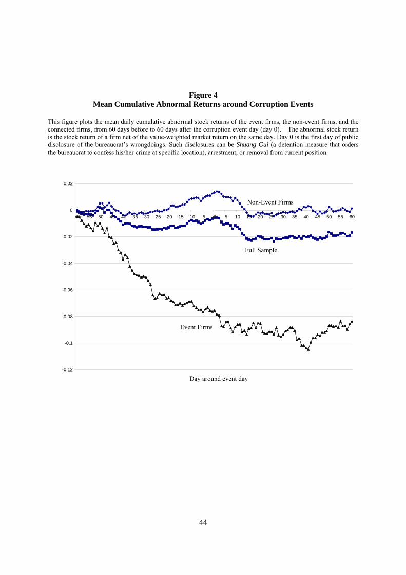
44

Figure 4 Mean Cumulative Abnormal Returns around Corruption Events

This figure plots the mean daily cumulative abnormal stock returns of the event firms, the non-event firms, and the connected firms, from 60 days before to 60 days after the corruption event day (day 0). The abnormal stock return is the stock return of a firm net of the value-weighted market return on the same day. Day 0 is the first day of public disclosure of the bureaucrat’s wrongdoings. Such disclosures can be Shuang Gui (a detention measure that orders the bureaucrat to confess his/her crime at specific location), arrestment, or removal from current position.

-0.12

-0.1

-0.08

-0.06

-0.04

-0.02

0

0.02

-60 -55 -50 -45 -40 -35 -30 -25 -20 -15 -10 -5 0 5 10 15 20 25 30 35 40 45 50 55 60

Day around event day

Non-Event Firms

Event Firms

Full Sample

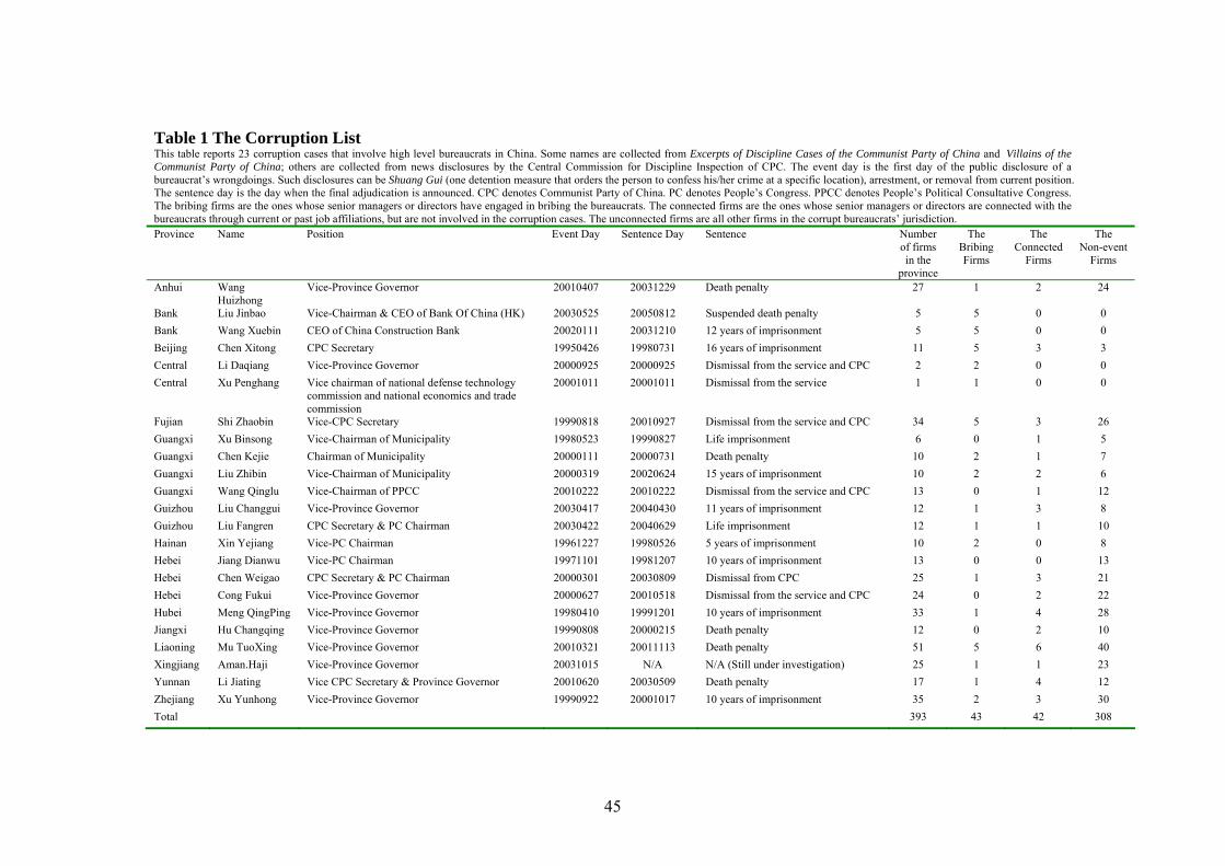
45

Table 1 The Corruption List This table reports 23 corruption cases that involve high level bureaucrats in China. Some names are collected from Excerpts of Discipline Cases of the Communist Party of China and Villains of the Communist Party of China; others are collected from news disclosures by the Central Commission for Discipline Inspection of CPC. The event day is the first day of the public disclosure of a bureaucrat’s wrongdoings. Such disclosures can be Shuang Gui (one detention measure that orders the person to confess his/her crime at a specific location), arrestment, or removal from current position. The sentence day is the day when the final adjudication is announced. CPC denotes Communist Party of China. PC denotes People’s Congress. PPCC denotes People’s Political Consultative Congress. The bribing firms are the ones whose senior managers or directors have engaged in bribing the bureaucrats. The connected firms are the ones whose senior managers or directors are connected with the bureaucrats through current or past job affiliations, but are not involved in the corruption cases. The unconnected firms are all other firms in the corrupt bureaucrats’ jurisdiction. Province Name Position Event Day Sentence Day Sentence Number

of firms in the

province

The Bribing Firms

The Connected

Firms

The Non-event

Firms

Anhui Wang Huizhong

Vice-Province Governor 20010407 20031229 Death penalty 27 1 2 24

Bank Liu Jinbao Vice-Chairman & CEO of Bank Of China (HK) 20030525 20050812 Suspended death penalty 5 5 0 0 Bank Wang Xuebin CEO of China Construction Bank 20020111 20031210 12 years of imprisonment 5 5 0 0 Beijing Chen Xitong CPC Secretary 19950426 19980731 16 years of imprisonment 11 5 3 3 Central Li Daqiang Vice-Province Governor 20000925 20000925 Dismissal from the service and CPC 2 2 0 0 Central Xu Penghang Vice chairman of national defense technology

commission and national economics and trade commission

20001011 20001011 Dismissal from the service 1 1 0 0

Fujian Shi Zhaobin Vice-CPC Secretary 19990818 20010927 Dismissal from the service and CPC 34 5 3 26 Guangxi Xu Binsong Vice-Chairman of Municipality 19980523 19990827 Life imprisonment 6 0 1 5 Guangxi Chen Kejie Chairman of Municipality 20000111 20000731 Death penalty 10 2 1 7 Guangxi Liu Zhibin Vice-Chairman of Municipality 20000319 20020624 15 years of imprisonment 10 2 2 6 Guangxi Wang Qinglu Vice-Chairman of PPCC 20010222 20010222 Dismissal from the service and CPC 13 0 1 12 Guizhou Liu Changgui Vice-Province Governor 20030417 20040430 11 years of imprisonment 12 1 3 8 Guizhou Liu Fangren CPC Secretary & PC Chairman 20030422 20040629 Life imprisonment 12 1 1 10 Hainan Xin Yejiang Vice-PC Chairman 19961227 19980526 5 years of imprisonment 10 2 0 8 Hebei Jiang Dianwu Vice-PC Chairman 19971101 19981207 10 years of imprisonment 13 0 0 13 Hebei Chen Weigao CPC Secretary & PC Chairman 20000301 20030809 Dismissal from CPC 25 1 3 21 Hebei Cong Fukui Vice-Province Governor 20000627 20010518 Dismissal from the service and CPC 24 0 2 22 Hubei Meng QingPing Vice-Province Governor 19980410 19991201 10 years of imprisonment 33 1 4 28 Jiangxi Hu Changqing Vice-Province Governor 19990808 20000215 Death penalty 12 0 2 10 Liaoning Mu TuoXing Vice-Province Governor 20010321 20011113 Death penalty 51 5 6 40 Xingjiang Aman.Haji Vice-Province Governor 20031015 N/A N/A (Still under investigation) 25 1 1 23 Yunnan Li Jiating Vice CPC Secretary & Province Governor 20010620 20030509 Death penalty 17 1 4 12 Zhejiang Xu Yunhong Vice-Province Governor 19990922 20001017 10 years of imprisonment 35 2 3 30 Total 393 43 42 308

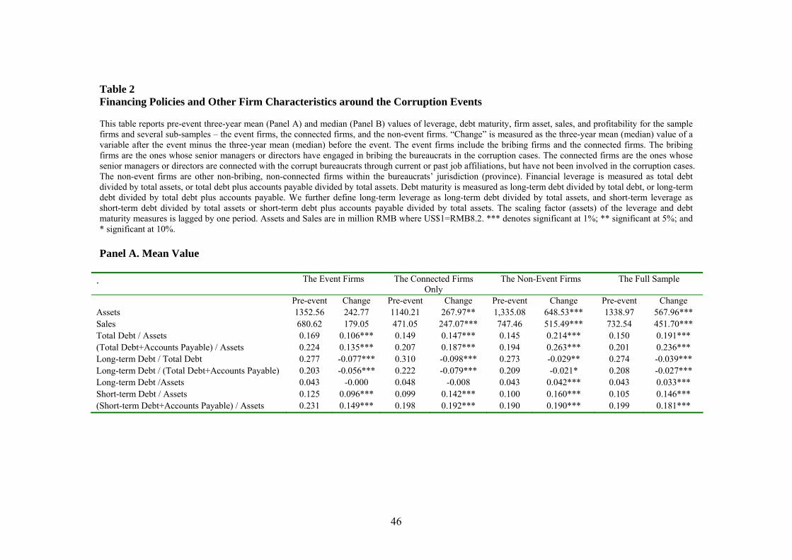
46

Table 2 Financing Policies and Other Firm Characteristics around the Corruption Events This table reports pre-event three-year mean (Panel A) and median (Panel B) values of leverage, debt maturity, firm asset, sales, and profitability for the sample firms and several sub-samples – the event firms, the connected firms, and the non-event firms. “Change” is measured as the three-year mean (median) value of a variable after the event minus the three-year mean (median) before the event. The event firms include the bribing firms and the connected firms. The bribing firms are the ones whose senior managers or directors have engaged in bribing the bureaucrats in the corruption cases. The connected firms are the ones whose senior managers or directors are connected with the corrupt bureaucrats through current or past job affiliations, but have not been involved in the corruption cases. The non-event firms are other non-bribing, non-connected firms within the bureaucrats’ jurisdiction (province). Financial leverage is measured as total debt divided by total assets, or total debt plus accounts payable divided by total assets. Debt maturity is measured as long-term debt divided by total debt, or long-term debt divided by total debt plus accounts payable. We further define long-term leverage as long-term debt divided by total assets, and short-term leverage as short-term debt divided by total assets or short-term debt plus accounts payable divided by total assets. The scaling factor (assets) of the leverage and debt maturity measures is lagged by one period. Assets and Sales are in million RMB where US$1=RMB8.2. *** denotes significant at 1%; ** significant at 5%; and * significant at 10%. Panel A. Mean Value

. The Event Firms The Connected Firms Only

The Non-Event Firms The Full Sample

Pre-event Change Pre-event Change Pre-event Change Pre-event Change Assets 1352.56 242.77 1140.21 267.97** 1,335.08 648.53*** 1338.97 567.96*** Sales 680.62 179.05 471.05 247.07*** 747.46 515.49*** 732.54 451.70*** Total Debt / Assets 0.169 0.106*** 0.149 0.147*** 0.145 0.214*** 0.150 0.191*** (Total Debt+Accounts Payable) / Assets 0.224 0.135*** 0.207 0.187*** 0.194 0.263*** 0.201 0.236*** Long-term Debt / Total Debt 0.277 -0.077*** 0.310 -0.098*** 0.273 -0.029** 0.274 -0.039*** Long-term Debt / (Total Debt+Accounts Payable) 0.203 -0.056*** 0.222 -0.079*** 0.209 -0.021* 0.208 -0.027*** Long-term Debt /Assets 0.043 -0.000 0.048 -0.008 0.043 0.042*** 0.043 0.033*** Short-term Debt / Assets 0.125 0.096*** 0.099 0.142*** 0.100 0.160*** 0.105 0.146*** (Short-term Debt+Accounts Payable) / Assets 0.231 0.149*** 0.198 0.192*** 0.190 0.190*** 0.199 0.181***

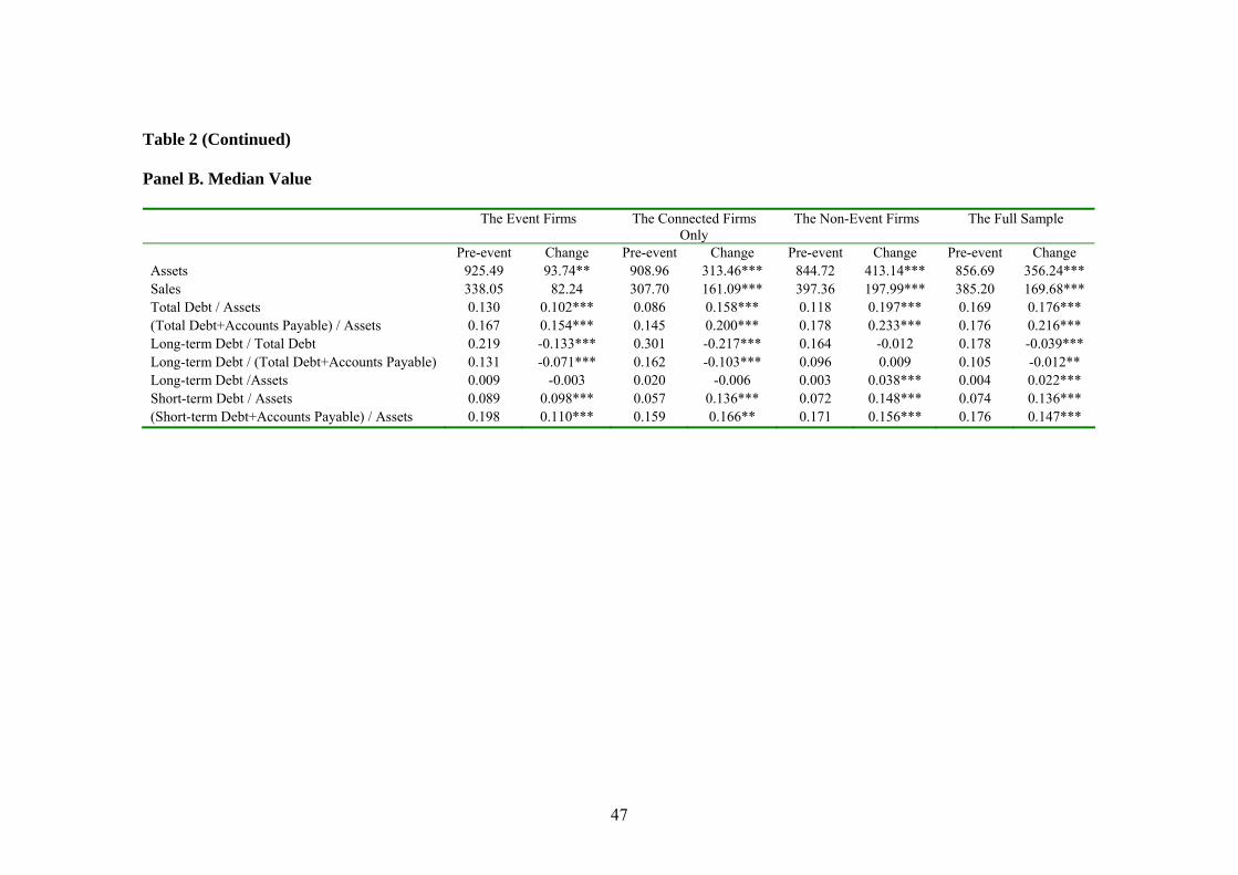
47

Table 2 (Continued) Panel B. Median Value The Event Firms The Connected Firms

Only The Non-Event Firms The Full Sample

Pre-event Change Pre-event Change Pre-event Change Pre-event Change Assets 925.49 93.74** 908.96 313.46*** 844.72 413.14*** 856.69 356.24***Sales 338.05 82.24 307.70 161.09*** 397.36 197.99*** 385.20 169.68***Total Debt / Assets 0.130 0.102*** 0.086 0.158*** 0.118 0.197*** 0.169 0.176*** (Total Debt+Accounts Payable) / Assets 0.167 0.154*** 0.145 0.200*** 0.178 0.233*** 0.176 0.216*** Long-term Debt / Total Debt 0.219 -0.133*** 0.301 -0.217*** 0.164 -0.012 0.178 -0.039***Long-term Debt / (Total Debt+Accounts Payable) 0.131 -0.071*** 0.162 -0.103*** 0.096 0.009 0.105 -0.012** Long-term Debt /Assets 0.009 -0.003 0.020 -0.006 0.003 0.038*** 0.004 0.022*** Short-term Debt / Assets 0.089 0.098*** 0.057 0.136*** 0.072 0.148*** 0.074 0.136*** (Short-term Debt+Accounts Payable) / Assets 0.198 0.110*** 0.159 0.166** 0.171 0.156*** 0.176 0.147***

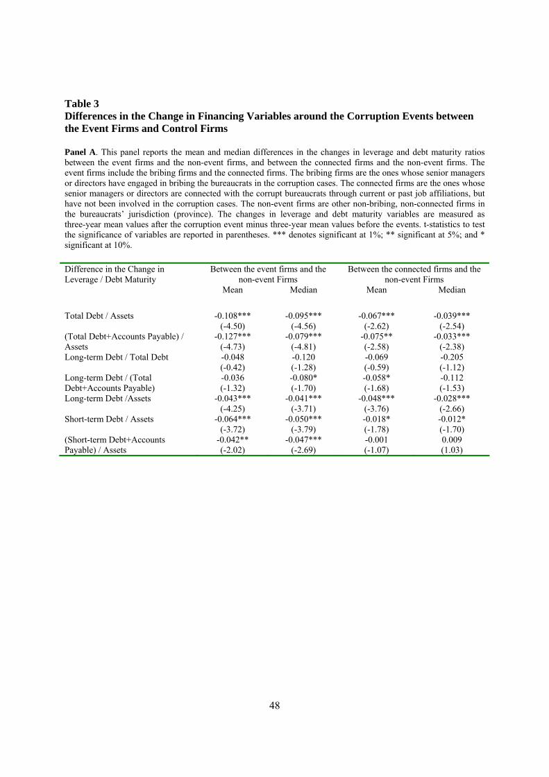
48

Table 3 Differences in the Change in Financing Variables around the Corruption Events between the Event Firms and Control Firms

Panel A. This panel reports the mean and median differences in the changes in leverage and debt maturity ratios between the event firms and the non-event firms, and between the connected firms and the non-event firms. The event firms include the bribing firms and the connected firms. The bribing firms are the ones whose senior managers or directors have engaged in bribing the bureaucrats in the corruption cases. The connected firms are the ones whose senior managers or directors are connected with the corrupt bureaucrats through current or past job affiliations, but have not been involved in the corruption cases. The non-event firms are other non-bribing, non-connected firms in the bureaucrats’ jurisdiction (province). The changes in leverage and debt maturity variables are measured as three-year mean values after the corruption event minus three-year mean values before the events. t-statistics to test the significance of variables are reported in parentheses. *** denotes significant at 1%; ** significant at 5%; and * significant at 10%. Difference in the Change in Leverage / Debt Maturity

Between the event firms and the non-event Firms

Between the connected firms and the non-event Firms

Mean Median Mean Median

Total Debt / Assets

-0.108*** (-4.50)

-0.095*** (-4.56)

-0.067*** (-2.62)

-0.039*** (-2.54)

(Total Debt+Accounts Payable) / Assets

-0.127*** (-4.73)

-0.079*** (-4.81)

-0.075** (-2.58)

-0.033*** (-2.38)

Long-term Debt / Total Debt -0.048 (-0.42)

-0.120 (-1.28)

-0.069 (-0.59)

-0.205 (-1.12)

Long-term Debt / (Total Debt+Accounts Payable)

-0.036 (-1.32)

-0.080* (-1.70)

-0.058* (-1.68)

-0.112 (-1.53)

Long-term Debt /Assets -0.043*** (-4.25)

-0.041*** (-3.71)

-0.048*** (-3.76)

-0.028*** (-2.66)

Short-term Debt / Assets -0.064*** (-3.72)

-0.050*** (-3.79)

-0.018* (-1.78)

-0.012* (-1.70)

(Short-term Debt+Accounts Payable) / Assets

-0.042** (-2.02)

-0.047*** (-2.69)

-0.001 (-1.07)

0.009 (1.03)

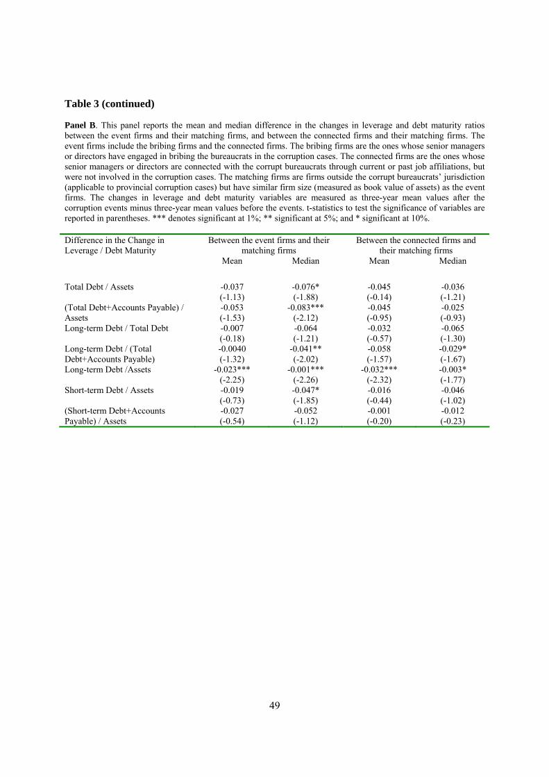
49

Table 3 (continued)

Panel B. This panel reports the mean and median difference in the changes in leverage and debt maturity ratios between the event firms and their matching firms, and between the connected firms and their matching firms. The event firms include the bribing firms and the connected firms. The bribing firms are the ones whose senior managers or directors have engaged in bribing the bureaucrats in the corruption cases. The connected firms are the ones whose senior managers or directors are connected with the corrupt bureaucrats through current or past job affiliations, but were not involved in the corruption cases. The matching firms are firms outside the corrupt bureaucrats’ jurisdiction (applicable to provincial corruption cases) but have similar firm size (measured as book value of assets) as the event firms. The changes in leverage and debt maturity variables are measured as three-year mean values after the corruption events minus three-year mean values before the events. t-statistics to test the significance of variables are reported in parentheses. *** denotes significant at 1%; ** significant at 5%; and * significant at 10%. Difference in the Change in Leverage / Debt Maturity

Between the event firms and their matching firms

Between the connected firms and their matching firms

Mean Median Mean Median

Total Debt / Assets

-0.037 (-1.13)

-0.076* (-1.88)

-0.045 (-0.14)

-0.036 (-1.21)

(Total Debt+Accounts Payable) / Assets

-0.053 (-1.53)

-0.083*** (-2.12)

-0.045 (-0.95)

-0.025 (-0.93)

Long-term Debt / Total Debt

-0.007 (-0.18)

-0.064 (-1.21)

-0.032 (-0.57)

-0.065 (-1.30)

Long-term Debt / (Total Debt+Accounts Payable)

-0.0040 (-1.32)

-0.041** (-2.02)

-0.058 (-1.57)

-0.029* (-1.67)

Long-term Debt /Assets

-0.023*** (-2.25)

-0.001*** (-2.26)

-0.032*** (-2.32)

-0.003* (-1.77)

Short-term Debt / Assets

-0.019 (-0.73)

-0.047* (-1.85)

-0.016 (-0.44)

-0.046 (-1.02)

(Short-term Debt+Accounts Payable) / Assets

-0.027 (-0.54)

-0.052 (-1.12)

-0.001 (-0.20)

-0.012 (-0.23)

50

Table 4 Mean Regression Results of the Effects of Corruption Cases on the Event Firms’ Leverage and Debt Maturity Ratios This panel reports the mean regression results of the impact of the corruption events on firm’s leverage and debt maturity. The ordinary least squared method is employed in the regressions. For each variable included, we compute its three-year mean value before and after the event. Panel A reports regression results based on the event firms and the non-event firms. Panel B reports results based on the event firms and the matching firms. The matching firms are firms outside the corrupt bureaucrats’ jurisdiction but have similar firm size (measured as book value of assets) as the event firms. The dependent variables are the various measures of leverage and debt maturity as defined in Table 2. The independent variables include the following: a dummy variable “Corrupt” equal 1 if the firm is an event firm, and otherwise 0; a dummy variable “Post” equal 1 if it is after the event year, and 0 if it is prior to the event year; “Lass” measured as log of assets; the interaction term of “Corrupt” and “Post”, tangible assets as a ratio of assets (“Tangible”); “Growth” measured as the market value of equity over book value of equity; and return on assets (“Profit”). Industry dummy variables are included in the regressions but their coefficients are not reported in this table. N is the number of observations. t-statistics are in parentheses. *** denotes significant at 1%; ** significant at 5%; and * significant at 10%. Panel A. Benchmarked against the Non-event Firms

Dependent Variable

Total Debt/Assets

(Total Debt+Accounts Payable)/Assets

Long-term Debt/Total Debt

Long-term Debt/(Total

Debt+Accounts Payable)

Long-term Debt/Assets

Short-term Debt/Assets

(Short-term Debt+Accounts Payable)/Assets

Intercept -0.644*** -0.879*** -0.908*** -0.744*** -0.475*** -0.097 -0.380** (-3.78) (-4.64) (-5.03) (-5.04) (-7.23) (-0.71) (-2.06)

Corrupt 0.038* 0.046* 0.025 0.018 0.005 0.034* 0.025 (1.66) (1.76) (1.01) (0.88) (0.58) (1.79) (1.00)

Post 0.176*** 0.221*** -0.033* -0.027* 0.019*** 0.152*** 0.182*** (11.04) (12.47) (-1.95) (-1.94) (3.02) (11.75) (10.60)

Corrupt*Post -0.100*** -0.118*** -0.038* -0.039* -0.031*** -0.070*** -0.068* (-3.04) (-3.22) (-1.78) (-1.66) (-2.47) (-2.64) (-1.91)

Lass 0.038*** 0.054*** 0.041*** 0.032*** 0.021*** 0.014** 0.036*** (4.55) (5.82) (4.62) (4.47) (6.60) (2.03) (4.01)

Tangible 0.179*** 0.107*** 0.528*** 0.466*** 0.170*** -0.029 -0.172*** (4.07) (2.18) (11.28) (12.17) (9.97) (-0.82) (-3.61)

Sales Growth 0.172*** 0.203*** 0.018 0.011 0.025* 0.130*** 0.168*** (4.70) (4.98) (0.46) (0.36) (1.74) (4.38) (4.25)

Profit -0.450*** -0.312** 0.045 -0.107 -0.171*** -0.220** -0.394*** (-3.28) (-2.05) (0.31) (-0.90) (-3.23) (-1.98) (-2.66)

N 746 739 721 739 746 746 739 Adj R-squared 29.0% 32.7% 24.0% 25.3% 25.2% 26.7% 26.1%

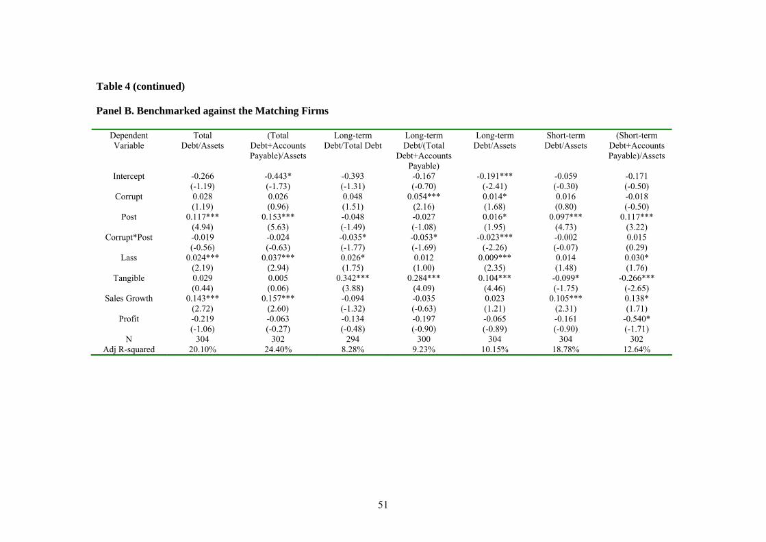
51

Table 4 (continued) Panel B. Benchmarked against the Matching Firms

Dependent Variable

Total Debt/Assets

(Total Debt+Accounts Payable)/Assets

Long-term Debt/Total Debt

Long-term Debt/(Total

Debt+Accounts Payable)

Long-term Debt/Assets

Short-term Debt/Assets

(Short-term Debt+Accounts Payable)/Assets

Intercept -0.266 -0.443* -0.393 -0.167 -0.191*** -0.059 -0.171 (-1.19) (-1.73) (-1.31) (-0.70) (-2.41) (-0.30) (-0.50)

Corrupt 0.028 0.026 0.048 0.054*** 0.014* 0.016 -0.018 (1.19) (0.96) (1.51) (2.16) (1.68) (0.80) (-0.50)

Post 0.117*** 0.153*** -0.048 -0.027 0.016* 0.097*** 0.117*** (4.94) (5.63) (-1.49) (-1.08) (1.95) (4.73) (3.22)

Corrupt*Post -0.019 -0.024 -0.035* -0.053* -0.023*** -0.002 0.015 (-0.56) (-0.63) (-1.77) (-1.69) (-2.26) (-0.07) (0.29)

Lass 0.024*** 0.037*** 0.026* 0.012 0.009*** 0.014 0.030* (2.19) (2.94) (1.75) (1.00) (2.35) (1.48) (1.76)

Tangible 0.029 0.005 0.342*** 0.284*** 0.104*** -0.099* -0.266*** (0.44) (0.06) (3.88) (4.09) (4.46) (-1.75) (-2.65)

Sales Growth 0.143*** 0.157*** -0.094 -0.035 0.023 0.105*** 0.138* (2.72) (2.60) (-1.32) (-0.63) (1.21) (2.31) (1.71)

Profit -0.219 -0.063 -0.134 -0.197 -0.065 -0.161 -0.540* (-1.06) (-0.27) (-0.48) (-0.90) (-0.89) (-0.90) (-1.71)

N 304 302 294 300 304 304 302 Adj R-squared 20.10% 24.40% 8.28% 9.23% 10.15% 18.78% 12.64%

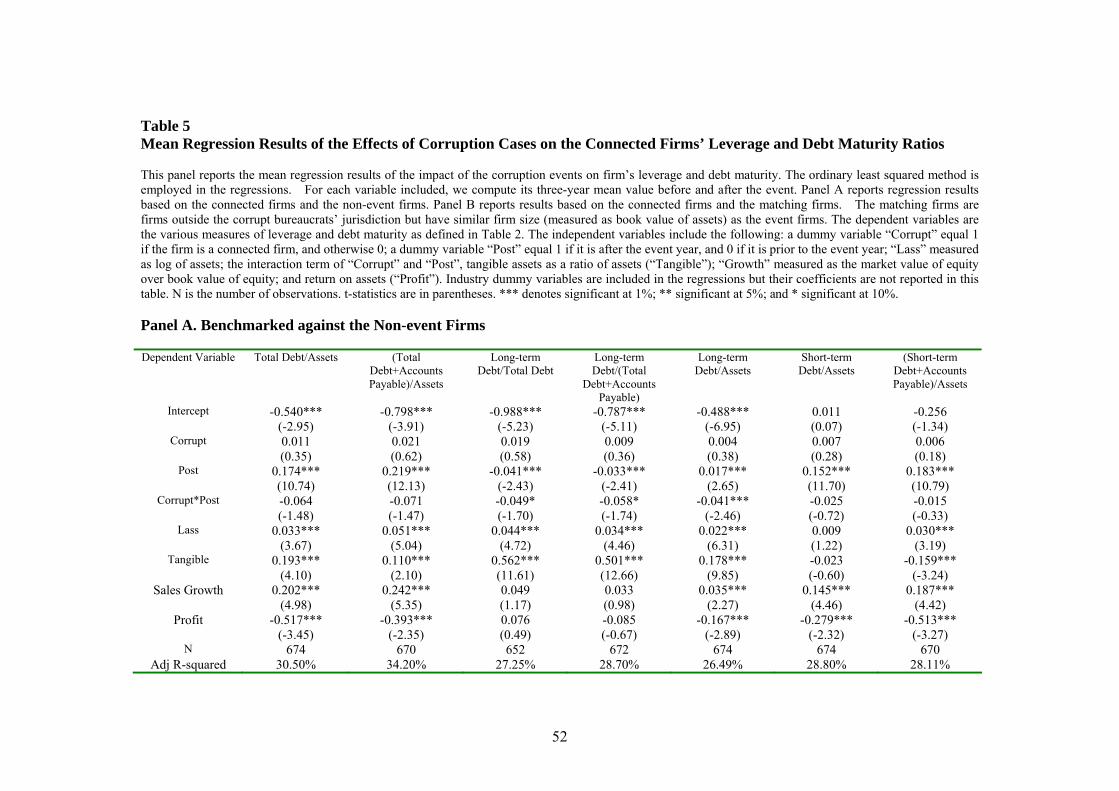
52

Table 5 Mean Regression Results of the Effects of Corruption Cases on the Connected Firms’ Leverage and Debt Maturity Ratios This panel reports the mean regression results of the impact of the corruption events on firm’s leverage and debt maturity. The ordinary least squared method is employed in the regressions. For each variable included, we compute its three-year mean value before and after the event. Panel A reports regression results based on the connected firms and the non-event firms. Panel B reports results based on the connected firms and the matching firms. The matching firms are firms outside the corrupt bureaucrats’ jurisdiction but have similar firm size (measured as book value of assets) as the event firms. The dependent variables are the various measures of leverage and debt maturity as defined in Table 2. The independent variables include the following: a dummy variable “Corrupt” equal 1 if the firm is a connected firm, and otherwise 0; a dummy variable “Post” equal 1 if it is after the event year, and 0 if it is prior to the event year; “Lass” measured as log of assets; the interaction term of “Corrupt” and “Post”, tangible assets as a ratio of assets (“Tangible”); “Growth” measured as the market value of equity over book value of equity; and return on assets (“Profit”). Industry dummy variables are included in the regressions but their coefficients are not reported in this table. N is the number of observations. t-statistics are in parentheses. *** denotes significant at 1%; ** significant at 5%; and * significant at 10%. Panel A. Benchmarked against the Non-event Firms Dependent Variable Total Debt/Assets (Total

Debt+Accounts Payable)/Assets

Long-term Debt/Total Debt

Long-term Debt/(Total

Debt+Accounts Payable)

Long-term Debt/Assets

Short-term Debt/Assets

(Short-term Debt+Accounts Payable)/Assets

Intercept -0.540*** -0.798*** -0.988*** -0.787*** -0.488*** 0.011 -0.256 (-2.95) (-3.91) (-5.23) (-5.11) (-6.95) (0.07) (-1.34)

Corrupt 0.011 0.021 0.019 0.009 0.004 0.007 0.006 (0.35) (0.62) (0.58) (0.36) (0.38) (0.28) (0.18)

Post 0.174*** 0.219*** -0.041*** -0.033*** 0.017*** 0.152*** 0.183*** (10.74) (12.13) (-2.43) (-2.41) (2.65) (11.70) (10.79)

Corrupt*Post -0.064 -0.071 -0.049* -0.058* -0.041*** -0.025 -0.015 (-1.48) (-1.47) (-1.70) (-1.74) (-2.46) (-0.72) (-0.33)

Lass 0.033*** 0.051*** 0.044*** 0.034*** 0.022*** 0.009 0.030*** (3.67) (5.04) (4.72) (4.46) (6.31) (1.22) (3.19)

Tangible 0.193*** 0.110*** 0.562*** 0.501*** 0.178*** -0.023 -0.159*** (4.10) (2.10) (11.61) (12.66) (9.85) (-0.60) (-3.24)

Sales Growth 0.202*** 0.242*** 0.049 0.033 0.035*** 0.145*** 0.187*** (4.98) (5.35) (1.17) (0.98) (2.27) (4.46) (4.42)

Profit -0.517*** -0.393*** 0.076 -0.085 -0.167*** -0.279*** -0.513*** (-3.45) (-2.35) (0.49) (-0.67) (-2.89) (-2.32) (-3.27)

N 674 670 652 672 674 674 670 Adj R-squared 30.50% 34.20% 27.25% 28.70% 26.49% 28.80% 28.11%

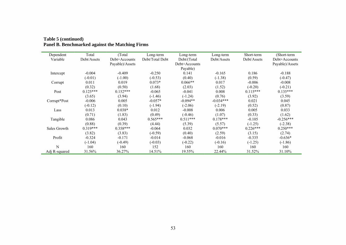
53

Table 5 (continued) Panel B. Benchmarked against the Matching Firms

Dependent Variable

Total Debt/Assets

(Total Debt+Accounts Payable)/Assets

Long-term Debt/Total Debt

Long-term Debt/(Total

Debt+Accounts Payable)

Long-term Debt/Assets

Short-term Debt/Assets

(Short-term Debt+Accounts Payable)/Assets

Intercept -0.004 -0.409 -0.250 0.141 -0.165 0.186 -0.188 (-0.01) (-1.00) (-0.53) (0.40) (-1.38) (0.59) (-0.47)

Corrupt 0.011 0.019 0.073* 0.066** 0.017 -0.006 -0.008 (0.32) (0.50) (1.68) (2.03) (1.52) (-0.20) (-0.21)

Post 0.125*** 0.152*** -0.065 -0.041 0.008 0.115*** 0.135*** (3.65) (3.94) (-1.46) (-1.24) (0.76) (3.92) (3.59)

Corrupt*Post -0.006 0.005 -0.057* -0.094** -0.034*** 0.021 0.045 (-0.12) (0.10) (-1.94) (-2.06) (-2.19) (0.52) (0.87)

Lass 0.013 0.038* 0.012 -0.008 0.006 0.005 0.033 (0.71) (1.83) (0.49) (-0.46) (1.07) (0.33) (1.62)

Tangible 0.086 0.043 0.565*** 0.511*** 0.178*** -0.105 -0.256*** (0.88) (0.39) (4.44) (5.39) (5.57) (-1.25) (-2.38)

Sales Growth 0.319*** 0.358*** -0.064 0.032 0.070*** 0.226*** 0.250*** (3.82) (3.83) (-0.59) (0.40) (2.59) (3.15) (2.74)

Profit -0.324 -0.171 -0.014 -0.068 -0.016 -0.335 -0.636* (-1.04) (-0.49) (-0.03) (-0.22) (-0.16) (-1.25) (-1.86)

N 160 160 152 160 160 160 160 Adj R-squared 31.56% 36.27% 14.51% 19.55% 22.44% 31.52% 31.10%

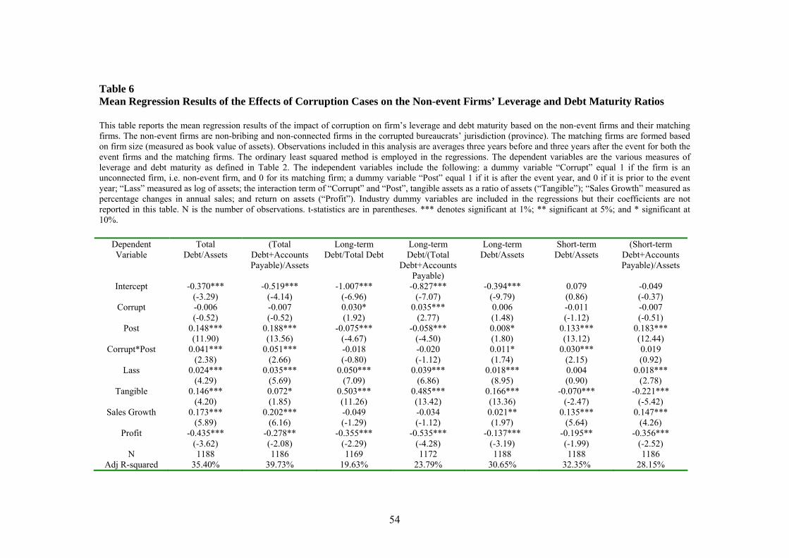
54

Table 6 Mean Regression Results of the Effects of Corruption Cases on the Non-event Firms’ Leverage and Debt Maturity Ratios This table reports the mean regression results of the impact of corruption on firm’s leverage and debt maturity based on the non-event firms and their matching firms. The non-event firms are non-bribing and non-connected firms in the corrupted bureaucrats’ jurisdiction (province). The matching firms are formed based on firm size (measured as book value of assets). Observations included in this analysis are averages three years before and three years after the event for both the event firms and the matching firms. The ordinary least squared method is employed in the regressions. The dependent variables are the various measures of leverage and debt maturity as defined in Table 2. The independent variables include the following: a dummy variable “Corrupt” equal 1 if the firm is an unconnected firm, i.e. non-event firm, and 0 for its matching firm; a dummy variable “Post” equal 1 if it is after the event year, and 0 if it is prior to the event year; “Lass” measured as log of assets; the interaction term of “Corrupt” and “Post”, tangible assets as a ratio of assets (“Tangible”); “Sales Growth” measured as percentage changes in annual sales; and return on assets (“Profit”). Industry dummy variables are included in the regressions but their coefficients are not reported in this table. N is the number of observations. t-statistics are in parentheses. *** denotes significant at 1%; ** significant at 5%; and * significant at 10%.

Dependent Variable

Total Debt/Assets

(Total Debt+Accounts Payable)/Assets

Long-term Debt/Total Debt

Long-term Debt/(Total

Debt+Accounts Payable)

Long-term Debt/Assets

Short-term Debt/Assets

(Short-term Debt+Accounts Payable)/Assets

Intercept -0.370*** -0.519*** -1.007*** -0.827*** -0.394*** 0.079 -0.049 (-3.29) (-4.14) (-6.96) (-7.07) (-9.79) (0.86) (-0.37)

Corrupt -0.006 -0.007 0.030* 0.035*** 0.006 -0.011 -0.007 (-0.52) (-0.52) (1.92) (2.77) (1.48) (-1.12) (-0.51)

Post 0.148*** 0.188*** -0.075*** -0.058*** 0.008* 0.133*** 0.183*** (11.90) (13.56) (-4.67) (-4.50) (1.80) (13.12) (12.44)

Corrupt*Post 0.041*** 0.051*** -0.018 -0.020 0.011* 0.030*** 0.019 (2.38) (2.66) (-0.80) (-1.12) (1.74) (2.15) (0.92)

Lass 0.024*** 0.035*** 0.050*** 0.039*** 0.018*** 0.004 0.018*** (4.29) (5.69) (7.09) (6.86) (8.95) (0.90) (2.78)

Tangible 0.146*** 0.072* 0.503*** 0.485*** 0.166*** -0.070*** -0.221*** (4.20) (1.85) (11.26) (13.42) (13.36) (-2.47) (-5.42)

Sales Growth 0.173*** 0.202*** -0.049 -0.034 0.021** 0.135*** 0.147*** (5.89) (6.16) (-1.29) (-1.12) (1.97) (5.64) (4.26)

Profit -0.435*** -0.278** -0.355*** -0.535*** -0.137*** -0.195** -0.356*** (-3.62) (-2.08) (-2.29) (-4.28) (-3.19) (-1.99) (-2.52)

N 1188 1186 1169 1172 1188 1188 1186 Adj R-squared 35.40% 39.73% 19.63% 23.79% 30.65% 32.35% 28.15%

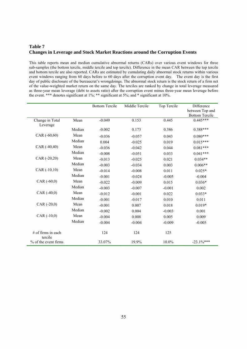
55

Table 7 Changes in Leverage and Stock Market Reactions around the Corruption Events This table reports mean and median cumulative abnormal returns (CARs) over various event windows for three sub-samples (the bottom tercile, middle tercile and top tercile). Difference in the mean CAR between the top tercile and bottom tercile are also reported. CARs are estimated by cumulating daily abnormal stock returns within various event windows ranging from 60 days before to 60 days after the corruption event day. The event day is the first day of public disclosure of the bureaucrat’s wrongdoings. The abnormal stock return is the stock return of a firm net of the value-weighted market return on the same day. The terciles are ranked by change in total leverage measured as three-year mean leverage (debt to assets ratio) after the corruption event minus three-year mean leverage before the event. *** denotes significant at 1%; ** significant at 5%; and * significant at 10%.

Bottom Tercile Middle Tercile Top Tercile Difference between Top and Bottom Tercile

Change in Total Leverage

Mean -0.049 0.153 0.445 0.445***

Median -0.002 0.173 0.386 0.388*** CAR (-60,60) Mean -0.036 -0.057 0.043 0.080***

Median 0.004 -0.025 0.019 0.015*** CAR (-40,40) Mean -0.036 -0.042 0.044 0.081***

Median -0.008 -0.051 0.033 0.041*** CAR (-20,20) Mean -0.013 -0.025 0.021 0.034**

Median -0.003 -0.034 0.003 0.006** CAR (-10,10) Mean -0.014 -0.008 0.011 0.025*

Median -0.001 -0.024 -0.005 -0.004 CAR (-60,0) Mean -0.022 -0.009 0.015 0.036*

Median -0.003 -0.007 -0.001 0.002 CAR (-40,0) Mean -0.012 -0.001 0.022 0.033*

Median -0.001 -0.017 0.010 0.011 CAR (-20,0) Mean -0.001 0.007 0.018 0.019*

Median -0.002 0.004 -0.003 0.001 CAR (-10,0) Mean -0.004 0.008 0.005 0.009

Median -0.004 -0.004 -0.009 -0.005

# of firms in each tercile

124 124 125

% of the event firms 33.07% 19.9% 10.0% -23.1%***

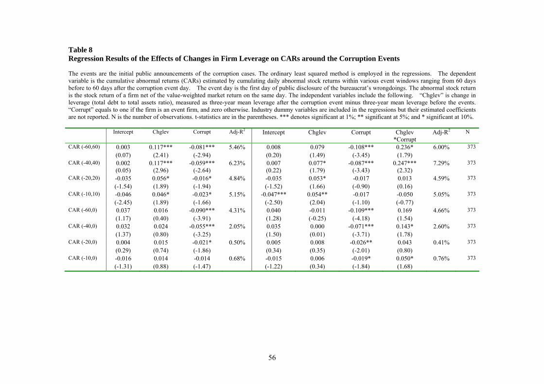
56

Table 8 Regression Results of the Effects of Changes in Firm Leverage on CARs around the Corruption Events

The events are the initial public announcements of the corruption cases. The ordinary least squared method is employed in the regressions. The dependent variable is the cumulative abnormal returns (CARs) estimated by cumulating daily abnormal stock returns within various event windows ranging from 60 days before to 60 days after the corruption event day. The event day is the first day of public disclosure of the bureaucrat’s wrongdoings. The abnormal stock return is the stock return of a firm net of the value-weighted market return on the same day. The independent variables include the following. “Chglev” is change in leverage (total debt to total assets ratio), measured as three-year mean leverage after the corruption event minus three-year mean leverage before the events. “Corrupt” equals to one if the firm is an event firm, and zero otherwise. Industry dummy variables are included in the regressions but their estimated coefficients are not reported. N is the number of observations. t-statistics are in the parentheses. *** denotes significant at 1%; ** significant at 5%; and * significant at 10%. Intercept Chglev Corrupt Adj-R2 Intercept Chglev Corrupt Chglev

*Corrupt Adj-R2 N

CAR (-60,60) 0.003 0.117*** -0.081*** 5.46% 0.008 0.079 -0.108*** 0.236* 6.00% 373 (0.07) (2.41) (-2.94) (0.20) (1.49) (-3.45) (1.79) CAR (-40,40) 0.002 0.117*** -0.059*** 6.23% 0.007 0.077* -0.087*** 0.247*** 7.29% 373 (0.05) (2.96) (-2.64) (0.22) (1.79) (-3.43) (2.32) CAR (-20,20) -0.035 0.056* -0.016* 4.84% -0.035 0.053* -0.017 0.013 4.59% 373 (-1.54) (1.89) (-1.94) (-1.52) (1.66) (-0.90) (0.16) CAR (-10,10) -0.046 0.046* -0.023* 5.15% -0.047*** 0.054** -0.017 -0.050 5.05% 373 (-2.45) (1.89) (-1.66) (-2.50) (2.04) (-1.10) (-0.77) CAR (-60,0) 0.037 0.016 -0.090*** 4.31% 0.040 -0.011 -0.109*** 0.169 4.66% 373 (1.17) (0.40) (-3.91) (1.28) (-0.25) (-4.18) (1.54) CAR (-40,0) 0.032 0.024 -0.055*** 2.05% 0.035 0.000 -0.071*** 0.143* 2.60% 373 (1.37) (0.80) (-3.25) (1.50) (0.01) (-3.71) (1.78) CAR (-20,0) 0.004 0.015 -0.021* 0.50% 0.005 0.008 -0.026** 0.043 0.41% 373 (0.29) (0.74) (-1.86) (0.34) (0.35) (-2.01) (0.80) CAR (-10,0) -0.016 0.014 -0.014 0.68% -0.015 0.006 -0.019* 0.050* 0.76% 373 (-1.31) (0.88) (-1.47) (-1.22) (0.34) (-1.84) (1.68)

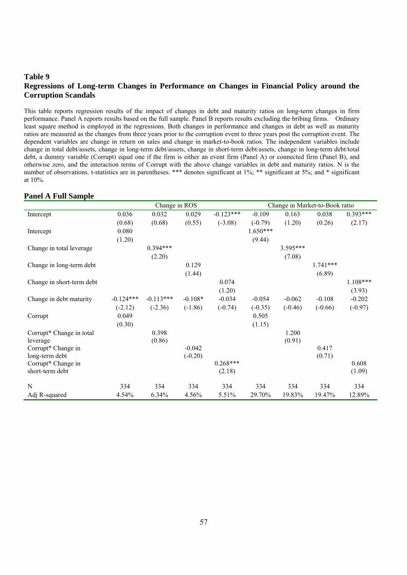
57

Table 9 Regressions of Long-term Changes in Performance on Changes in Financial Policy around the Corruption Scandals This table reports regression results of the impact of changes in debt and maturity ratios on long-term changes in firm performance. Panel A reports results based on the full sample. Panel B reports results excluding the bribing firms. Ordinary least square method is employed in the regressions. Both changes in performance and changes in debt as well as maturity ratios are measured as the changes from three years prior to the corruption event to three years post the corruption event. The dependent variables are change in return on sales and change in market-to-book ratios. The independent variables include change in total debt/assets, change in long-term debt/assets, change in short-term debt/assets, change in long-term debt/total debt, a dummy variable (Corrupt) equal one if the firm is either an event firm (Panel A) or connected firm (Panel B), and otherwise zero, and the interaction terms of Corrupt with the above change variables in debt and maturity ratios. N is the number of observations. t-statistics are in parentheses. *** denotes significant at 1%; ** significant at 5%; and * significant at 10%. Panel A Full Sample

Change in ROS Change in Market-to-Book ratio Intercept 0.036 0.032 0.029 -0.123*** -0.109 0.163 0.038 0.393*** (0.68) (0.68) (0.55) (-3.08) (-0.79) (1.20) (0.26) (2.17) Intercept 0.080 1.650*** (1.20) (9.44) Change in total leverage 0.394*** 3.595*** (2.20) (7.08) Change in long-term debt 0.129 1.741*** (1.44) (6.89) Change in short-term debt 0.074 1.108*** (1.20) (3.93) Change in debt maturity -0.124*** -0.113*** -0.108* -0.034 -0.054 -0.062 -0.108 -0.202 (-2.12) (-2.36) (-1.86) (-0.74) (-0.35) (-0.46) (-0.66) (-0.97) Corrupt 0.049 0.505 (0.30) (1.15) Corrupt* Change in total leverage

0.398 (0.86)

1.200 (0.91)

Corrupt* Change in long-term debt

-0.042 (-0.20)

0.417 (0.71)

Corrupt* Change in short-term debt

0.268***(2.18)

0.608 (1.09)

N 334 334 334 334 334 334 334 334 Adj R-squared 4.54% 6.34% 4.56% 5.51% 29.70% 19.83% 19.47% 12.89%

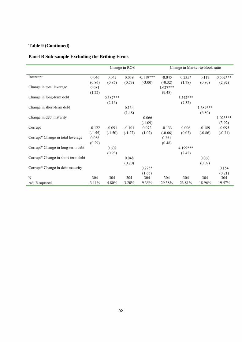
58

Table 9 (Continued)

Panel B Sub-sample Excluding the Bribing Firms Change in ROS

Change in Market-to-Book ratio

Intercept 0.046 0.042 0.039 -0.119*** -0.045 0.235* 0.117 0.502*** (0.86) (0.85) (0.73) (-3.00) (-0.32) (1.78) (0.80) (2.92) Change in total leverage 0.081 1.627*** (1.22) (9.48) Change in long-term debt 0.387*** 3.542*** (2.15) (7.32) Change in short-term debt 0.134 1.689*** (1.48) (6.80) Change in debt maturity -0.066 1.023*** (-1.09) (3.92) Corrupt -0.122 -0.091 -0.101 0.072 -0.133 0.006 -0.189 -0.095 (-1.55) (-1.50) (-1.27) (1.02) (-0.66) (0.03) (-0.86) (-0.31) Corrupt* Change in total leverage 0.058 0.251 (0.29) (0.48) Corrupt* Change in long-term debt 0.602 4.199*** (0.93) (2.42) Corrupt* Change in short-term debt 0.048 0.060 (0.20) (0.09) Corrupt* Change in debt maturity 0.275* 0.154 (1.65) (0.21) N 304 304 304 304 304 304 304 304 Adj R-squared 3.11% 4.80% 3.20% 9.35% 29.38% 23.81% 18.96% 19.57%

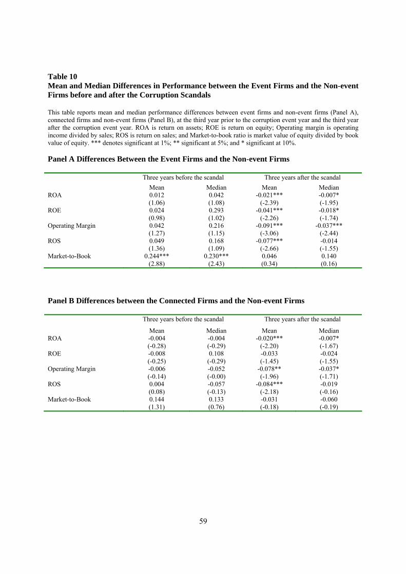
59

Table 10 Mean and Median Differences in Performance between the Event Firms and the Non-event Firms before and after the Corruption Scandals This table reports mean and median performance differences between event firms and non-event firms (Panel A), connected firms and non-event firms (Panel B), at the third year prior to the corruption event year and the third year after the corruption event year. ROA is return on assets; ROE is return on equity; Operating margin is operating income divided by sales; ROS is return on sales; and Market-to-book ratio is market value of equity divided by book value of equity. *** denotes significant at 1%; ** significant at 5%; and * significant at 10%. Panel A Differences Between the Event Firms and the Non-event Firms Three years before the scandal Three years after the scandal Mean Median Mean Median ROA 0.012

(1.06) 0.042 (1.08)

-0.021*** (-2.39)

-0.007* (-1.95)

ROE 0.024 (0.98)

0.293 (1.02)

-0.041*** (-2.26)

-0.018* (-1.74)

Operating Margin 0.042 (1.27)

0.216 (1.15)

-0.091*** (-3.06)

-0.037*** (-2.44)

ROS 0.049 (1.36)

0.168 (1.09)

-0.077*** (-2.66)

-0.014 (-1.55)

Market-to-Book 0.244*** (2.88)

0.230*** (2.43)

0.046 (0.34)

0.140 (0.16)

Panel B Differences between the Connected Firms and the Non-event Firms Three years before the scandal Three years after the scandal

Mean Median Mean Median ROA -0.004

(-0.28) -0.004 (-0.29)

-0.020*** (-2.20)

-0.007* (-1.67)

ROE -0.008 (-0.25)

0.108 (-0.29)

-0.033 (-1.45)

-0.024 (-1.55)

Operating Margin -0.006 (-0.14)

-0.052 (-0.00)

-0.078** (-1.96)

-0.037* (-1.71)

ROS 0.004 (0.08)

-0.057 (-0.13)

-0.084*** (-2.18)

-0.019 (-0.16)

Market-to-Book 0.144 (1.31)

0.133 (0.76)

-0.031 (-0.18)

-0.060 (-0.19)