Rent-Seeking in Elite Networks

Rainer Haselmann∗ David Schoenherr† Vikrant Vig ‡

April 14, 2016

Abstract

We employ a unique dataset on members of an elite service club in Germany toinvestigate how elite networks affect the allocation of resources. Specifically, we in-vestigate credit allocation decisions of banks to firms inside the network. Using aquasi-experimental research design, we document misallocation of bank credit insidethe network, with state-owned banks engaging most actively in crony lending. Theaggregate cost of credit misallocation amounts to 0.13 percent of annual GDP. Ourfindings, thus, resonate with existing theories of elite networks as rent extractive coali-tions that stifle economic prosperity.

JEL Codes: F34, F37, G21, G28, G33, K39.

∗SAFE and Goethe University Frankfurt. Email: haselmann@safe.uni-frankfurt.de†London Business School. Email: dschoenherr@london.edu‡London Business School and CEPR. Email: vvig@london.edu

We would like to thank Oriana Bandiera, Patrick Bolton, James Dow, Armin Falk, Neal Galpin, TarekHassan, Christian Hellwig, Ginger Zhe Jin, Matti Keloharju, Michael Kosfeld, Samuli Knupfer, StefanLewellen, Christopher Malloy, Ulrike Malmendier, Atif Mian, Jorn-Steffen Pischke, Ailsa Roell, StephenSchaefer, Kelly Shue, Rui Silva, David Thesmar, Alexander Wagner, Ivo Welch, and Luigi Zingales, as well asseminar and conference participants in Amsterdam, Berlin (HU), and Bonn, at the European Winter Financesummit, in Frankfurt, Glasgow, Helsinki, and Mainz, at the NBER, London Business School, London Schoolof Economics, Stockholm School of Economics, the University of Warwick, the Swiss Finance Association, andthe Western Finance Association for their helpful comments. We are grateful to the Deutsche Bundesbank,especially to Klaus Dullmann and Thomas Kick, for their generous support with the construction of the dataset. Haselmann thanks the Research Center SAFE, funded by the State of Hessen initiative for researchLOEWE for financial support. The usual disclaimer on errors applies here as well.

“People of the same trade seldom meet together, even for merriment and diver-

sion, but the conversation ends in a conspiracy against the public, or in some

contrivance to raise prices.”

Adam Smith, Wealth of Nations, 1776.

1 Introduction

In an insightful and thought-provoking book, entitled “Bowling Alone: The Collapse and

the Revival of American Economy”, Putnam (2000) made an important revelation about the

declining trend of social engagement in the American society. Using an enormous database,

Putnam documents that Americans today are less social and more disconnected from each

other than they were in the past. The advent of IT, the proliferation of mass media, changes

in family structures, increased mobility, and increased pressures on time and money have all

contributed to the changes in patterns of social engagement across the globe. Putnam (2000)

argues that this decline in social capital is detrimental for the well-being of the society, a

view that is supported by some influential recent research that documents the important role

of social capital in alleviating market frictions and thereby fostering economic development

(Knack and Keefer 1997; Guiso, Sapienza, and Zingales 2004; Karlan, Mobius, Rosenblat,

and Szeidl 2009).

However, social capital may not be unambiguously benign. In seminal work Olson (1982)

identifies the emergence of self-serving interest groups, collusive networks and lobbies that

are created to further their interests largely at the expense of broader economic prosperity.

Olson (1982) argues that, after a period of stable growth, countries have a tendency to accu-

mulate rent-extracting institutions that ultimately lead to the decline of nations. Compared

to more direct and visible forms of corruption in developing countries, those distributional in-

stitutions provide a means of a more subtle and disguised way of rent-extraction in developed

economies.1

Interestingly, during the same time period that is studied by Putnam, elite service club

organizations have bucked this declining trend and have continued to flourish (see Figure 1,

which plots the growth in membership to the largest two clubs in Germany). Membership

to those service clubs is considered prestigious and these clubs ensure exclusivity through

stringent member selection criteria. Typically, club members comprise local politicians, and

professional and business leaders. While the primary objective of these clubs is to raise

money to fight diseases, reduce poverty and educate people, there is a general perception

1This, according to Olson 1982, was the reason why Germany and Japan grew at a much faster rate thanBritain after the Second World War, which was saddled by these growth inhibiting collusive organizations.

1

that social connections established in the club are highly valuable to its members. Under

Putnam’s view the persistence and growth of these service clubs, despite a secular decline

in other forms of social engagement, would be a positive development. However, the service

clubs with their exclusive nature also bear resemblance with the ‘distributional’ institutions

described in Olson (1982).

In this paper, we examine the role of those elite networks in the allocation of resources

in the economy.2 Given their wide prevalence and their representation of a large share

of local political and business leaders a large fraction of resources is under the control of

service club members.3 Our focus here is on the allocation of credit between banks and firms

whose officials are members of this club. Specifically, we hand-collect data on members –

both firms’ CEOs and bank directors – for 211 service club branches, from 1993 to 2011,

to capture both cross-sectional and time series variation in social proximity, and we obtain

very detailed contract-level financial data on these members from the Deutsche Bundesbank.

We are thus able to create a unique dataset on social networks that provides very granular

information on social networks combined with detailed accounting information.

We focus on credit allocation for several reasons. First, efficient allocation of credit is an

important engine of economic growth (King and Levine 1993; Rajan and Zingales 1998). The

sheer magnitude of credit being allocated in these clubs makes it an important laboratory

to study. Second, data on bank lending is available at the very micro-level, allowing us to

exploit time-series and cross-sectional variation in detail. Finally, examining credit allocation

allows us to understand the mechanism that is at work. Asymmetric information and moral

hazard pose major impediments to financial contracting. Social capital between lenders

and borrowers is understood to relax informational constraints that adversely affect lending

(Guiso, Sapienza, and Zingales 2004), and improve enforcement by providing social collateral

(Karlan et al. 2009).4 On the other hand, consistent with the dark side view of social

capital, expressed by Olson (1982) and Adam Smith, social connections between borrowers

and lenders may generate new frictions from rent-seeking and favoritism that distort the

allocation of credit in the economy.

We find that banks misallocate credit inside the network, consistent with the dark side

view of social capital propagated by Olson (1982). The preferential allocation of credit takes

a rather subtle form. It does not come explicitly from observably lower interest rates, but

rather from excessive continuation of underperforming firms. Rough estimates of the overall

2Due to confidentiality reasons we are not able to disclose the name of the service club organization.3About five percent of all bank loans are extended within one such service club organization alone and are

therefore subject to the effects of social capital, generated through social interactions between bank directorsand firms’ CEOs in those club. Taking into account the total number of service club members in Germany,the share of bank loans contracted between club members is about 12.5 percent.

4Engelberg, Gao, and Parsons (2012) provide additional evidence in support of this view.

2

costs generated by preferential credit allocation inside the network suggest that the total

costs of capital misallocation amount to 0.13 to 0.19 percent of annual German GDP.

Despite the abundance of anecdotes on rent-seeking and collusion in social networks,

there is scant empirical evidence on this topic, especially when it comes to the allocation of

credit.5 This is certainly not because of its lack of importance; there is a growing recognition

that rent-seeking and collusion is ubiquitous and imposes substantial costs on the society.

However, empirically identifying such behavior has proven to be very difficult, as both the

bright-side (information and enforcement channels) and the dark-side views (collusion and

favoritism) generate observationally equivalent outcomes.

Economists have long struggled to distinguish empirically between taste-based (favoritism)

and statistical discrimination (Becker 1957; Arrow 1973; Phelps 1972). The challenge faced

by scholars in identifying rent-seeking behavior is very similar in spirit to the challenge re-

searchers face when trying to identify the presence of taste-based discrimination. To add to

this, researchers have to grapple with serious selection issues – formation of social networks

is not random and people often self-select into social groups that have interests aligned with

their own (Lazarsfeld and Merton 1954). In our context, firms whose CEO is part of a social

network might share characteristics that distinguish them from firms whose CEO is not part

of the same network. The main identification challenge is to isolate the impact of social

proximity from spurious effects caused by selection.

We tackle the endogenous selection issue in several ways. From the outset, it should

be noted that our analysis focuses on firms that are members of the same service club

organization. In other words, our analysis does not compare firms that are members of the

club with firms that are not members of the club. Instead, we compare firms whose CEOs are

members of the same club branch as the banker (referred to as in-group) with firms whose

CEOs are members of a different branch of the same service club in the same city (referred

to as out-group). Since members of this service club are selected with the same ideological

criteria, this should alleviate most selection concerns to a large extent. Moreover, the same

bank that is an in-group bank for one club branch, is an out-group bank for another club

branch. By comparing the same bank’s lending to firms whose CEOs are members of its

club branch with firms whose CEOs are not connected to the bank, we are able to control

for the time-invariant sources of unobserved bank heterogeneity.

To quantify the effect of social proximity on lending, our empirical strategy, which is

essentially a difference-in-differences methodology, compares for the same firm, quarter-by-

5Two notable exceptions are La Porta, Lopez-de Silanes, and Zamarripa (2003) who investigate thenegative consequences of related lending in Mexico and Khwaja and Mian (2005) who document the negativeeffects of political connections on lending in Pakistan.

3

quarter, the financing provided by in-group banks to that provided by out-group banks.

This empirical strategy thus controls for demand-side effects, such as changes in investment

opportunities. We begin our analysis by investigating two events that generate perturbation

in social proximity: 1) entry of new members to a club branch, and 2) formation of a new

club branch within a city.6 Entry of firms is driven by rules, such as the ‘one member per

industry’ rule. Thus, the entry of new members only takes place once their industry sector

slot becomes vacant (i.e., existing members retire). Similarly, the formation of a new club

branch, follows a highly regulated process that involves the agreements of a district extension

committee and the district governor. Since these events are driven by pre-defined rules, it

lends credibility to our research design. As will become evident, our analysis goes into great

depth in ensuring that the exclusion restrictions are not violated.

The main identification strategy exploits mayoral elections. In Germany, the mayor of

a district often directly becomes the local state bank’s supervisory board chairman.7 In his

capacity as a chairman of the supervisory board, the mayor commands a large influence

on the loan-granting activity of the bank, especially for corporate loans.8 So, while the

elected candidate is always a member of the club branch, the degree of influence changes

with the election. Importantly, the mayoral election is independent of time series changes

in firm characteristics. It is further independent of changes in bank quality that would be

of concern in case of bank entry. The mayoral election thus provides exogenous time series

variation in the members’ ability to access and approve funds, free from other influences.

The following facts emerge from our analysis. In-group banks have an 18.35 percent

higher market share among members of their own club branch, compared with members of

other branches in the same city. On average, entry to branches leads to an increase in the

fraction of total firm loans borrowed from the in-group bank by 10.03 percentage points. On

examining mayoral elections, we find that when a club member is elected as a mayor and

becomes the head of the local state bank, the share of loans from the state bank increases by

5.63 percentage points. The evidence on mayoral elections is reinforced by comparing firm

lending around mayoral elections for which the mayor is not appointed as the chairman of

the supervisory board of the local savings bank. Using this event as a placebo test, we can

isolate the effect of state bank proximity from the proximity to the mayor. If a club member

is elected as a mayor, but is not appointed as the head of the local state bank, there is no

effect on in-group financing. We further explore the dynamics of lending around these events

6Membership is offered to individuals. So when we state that a firm joins a club branch, it implies thatthe firm’s CEO joins a club branch.

7Whether the mayor is the chairman depends on the size of the city relative to the county. We discussthis issue in detail later in the paper.

8As a rule, decisions on large loans require approval by the credit committee (Kreditausschuss) which isoften chaired by the mayor.

4

and find that our results cannot be explained by pre-treatment trends.

We find that social proximity also significantly increases firms’ total debt by 32.22 percent.

This finding is confirmed when we examine branch formations and mayoral elections. On

examining the intensive and the extensive margins, we find that an increase in the degree of

social connectedness leads not only to more lending to firms that already have an existing

relationship with the in-group bank, but it also increases the probability of forming a new

relationship with this bank by 11.44 percent relative to out-group banks.

To evaluate the efficacy of resource allocation in elite networks, we calculate the return on

loans (ROL) that banks generate from in-group vis-a-vis out-group transactions. A simple

informational or enforcement theory should lead to a better allocation of credit, thereby

improving the ROL of the bank. A favoritism or a rent-seeking theory, on the other hand,

predicts that the ROL is lower for in-group compared to out-group loans originated by the

same bank. Since we are able to measure ex-post loan performance, all contract features

that affect the banks’ returns, e.g. differences in collateral, are accounted for. Thus, our

analysis is robust to differences in contract features.

We find that a given bank generates a 3.23 percentage points lower ROL on in-group

loans compared to out-group loans. In addition, the ROL of in-group banks is significantly

lower when compared to out-group banks for the same firm. Investigating the drivers of the

difference in ROL, we find that it mostly comes from the difference in returns generated from

lending to firms in financial distress. While interest rates and recovery rates on loans are not

much different for in-group loans compared to out-group loans, banks lend disproportionately

more to in-group firms that are closer to distress, and thus the banks lose a lot more when

these firms default. It should be noted that banks not only generate lower returns on

connected loans compared to other loans, but these loans earn returns well below the risk-

free rate and often the connected loan portfolio generates a negative ROL for the bank.

Furthermore, connected loans also exhibit higher return volatility. Clearly, such a pattern

cannot be rationalized by the action taken by a risk-averse lender who trades off ROL for

lower risk.

In addition to lower ROL for banks, the misallocation of credit in the economy induces

inefficiencies in the deployment of capital. An important role of banks is to screen firms with

profitable investment opportunities and allocate capital to its most profitable usage. This

link, however, breaks down when we look at in-group lending. Banks’ in-group financing is

less sensitive to firms’ investment opportunities compared to their out-group lending. This

distortion in banks’ capital allocation hinders credit to flow to the most profitable investment

projects, which in turn reduces the productivity of the economy. Examining how firms deploy

the extra financing they receive through their membership to the network, we find that firms

5

do not use the extra financing to make new investments, something one would expect if

social proximity to the lender relaxed financing constraints. Instead, firms use these funds

to increase payments to the shareholders, which in most cases means paying out to the CEO,

as most of these are relatively small, family-owned firms. Furthermore, the increase in bank

credit leads to a significant increase in leverage. The total loans to assets ratio increases by

6.17 percentage points after firms join the club.

We next investigate how the effects vary with bank ownership. Such a comparison across

different bank groups (private banks, state banks, cooperatives) allows us to examine the

effect of incentives and governance structures on the social proximity effect.9 We find that

entry of firms to a club branch increases their share of financing by 6.45 percentage points

more if the in-group bank is state-owned, compared to when this bank is privately-owned

or a cooperative. On examining the ROL, we find that, while the effects are present for

both state and private banks, the ROL effect is significantly stronger for state banks. More

specifically, the wedge in ROL obtained by the state banks for their in-group loans compared

with their out-group loans is significantly larger for state banks.10 Thus, state banks not

only grant more loans to firms in their network, but they also generate much lower ROL

within the branch. For cooperatives that present closest counterparts to state-owned savings

banks, we find a significantly weaker effect suggesting that better governance can mitigate

some of the ill effects of social proximity on lending (Bandiera, Barankay, and Rasul 2009).

These results are consistent with the view that state banks, due to blunt incentives, are more

likely to engage in crony lending.

This paper shows a dark side of social capital. By distorting the allocation of resources,

the presence of rent-seeking in elite social networks has the potential to cause significant dam-

age to the economy. The results in the paper are consistent with investment in rent-extracting

institutions by elite members of society (Acemoglu and Robinson 2008, 2012). While there

is abundant empirical evidence on the virtues of social capital in fostering economic develop-

ment (e.g., Knack and Keefer 1997; Guiso, Sapienza, and Zingales 2004), clear-cut empirical

evidence on a detrimental role of social capital in stifling economic efficiency is scarce, in

particular for developed economies with well-functioning institutions.11

9The key differences between state, private, and cooperative banks are detailed in Appendix B. In Ger-many, cooperative banks are organized similarly to state-owned banks sharing the same regional focus. Theownership structure, however, is quite different. Cooperatives are owned by their members, whereas savingsbanks are owned by the local government. The difference in ownership structure creates different incen-tives (Jensen and Meckling 1976), with cooperatives having a similar governance structure as private banks,whereas the governance in state-owned banks tends to be of lower quality (Engelmaier and Stowasser 2013).

10This test controls for differences in objective functions that might exist between state-owned andprivately-owned banks. Since we are looking at the wedge in ROL between in-group and out-group loans,for the same bank, we control for inherent differences in these different organizational forms.

11Satyanath, Voigtlander, and Voth (2013) show that dense networks of civic associations facilitated therise of the NS party in Germany.

6

The paper also contributes to a broader literature on social connections and economic

outcomes,12 as well as the literature on social proximity and bank lending. It is often argued

that proximity between banks and firms mitigates informational problems (Petersen and

Rajan 2002).13 Our results suggest that proximity can be a double-edged sword, and that

too much proximity may not always be desirable. La Porta, Lopez-de Silanes, and Zamarripa

(2003) investigate the negative consequences of related lending in Mexico, where related

lending is defined as loans to firms that are controlled and owned by the bank’s owners.

Similarly, Khwaja and Mian (2005) document the negative effects of political connections on

lending in Pakistan. There are two important differences between the findings in those papers

and our findings. First, the nature of connections is very different. In this paper, we examine

the effect of social connections, as opposed to ownership or political linkages. Second, as

La Porta, Lopez-de Silanes, and Zamarripa (2003) argue, it is not clear whether the negative

forces of related lending can be extrapolated to a developed economy, where corruption

and other institutional ills are perceived to be low. Our findings highlight that even in an

economy with developed institutions, social proximity generates sizeable distortions in credit

allocation.

Finally, our paper contributes to the understanding of the difference between state and

private financing (La Porta, Lopez-de Silanes, and Shleifer 2002). Governments around

the world are taking ownership of large parts of the banking system and, potentially, this

public-sector involvement in the banking sector may have considerable long-term effects on

all major industrialized countries.14

2 Institutional Background and Data

2.1 Service Clubs in Germany

To identify social capital, we focus on membership information of an important service club

organization in Germany. While the service club organization is organized through a global

headquarter in the United States, the individual service club branches operate locally in

12Granovetter (2005) describes the relationship between social connections and economic outcomes in thesociology literature; Shue (2013) discusses how executive peer networks affect managerial decision-makingand firm policies; Lerner and Malmendier (2011) examines social networks and entrepreneurship; Jacksonand Schneider (2010) document how social connections reduce moral hazard, Gompers, Mukharlyamov, andXuan (2012) find that venture capitalists make worse investment decisions when they share social traits;Burchardi and Hassan (2013) show that social connections influence economic growth.

13See also Mian (2006) and Fisman, Paravisini, and Vig (2012).14Several papers have documented distortions in lending by state-owned banks and state-regulated banking

sectors (Sapienza 2004). For theoretical evidence on this topic, see Krueger (1974) and Shleifer and Vishny(1993, 1994).

7

almost every city or county in Germany. The clubs bring together members, all of whom are

local business and professional leaders, to meet within their club branch once a week over

lunch or dinner to socialize. It is mandatory for each club member to attend the weekly

meetings on a regular basis to sustain membership.15 By frequently interacting during those

meetings, members built up social capital. While the stated objective of the service club is

to raise funds for charitable work, having personal connections to other business leaders is

often cited as an important membership perquisite.

A local club branch has about 50 members on average. Typically, there is one branch in

each city of about 20,000 inhabitants. In larger cities, formation of additional club branches

is common. There are about 1,000 club branches with about 50,000 members in Germany.

There are strict membership criteria new members have to fulfill that tend to be based on

business or professional leadership. Our sample area comprises all branches of the service

club organization in southern Germany (the northern boundary is Saarbruecken, Frankfurt,

Erfurt and Hof) during the period from 1993 to 2011.16 Further details on the data collection

are described in Appendix A. We gather membership information on all corporate CEOs and

directors of bank branches for 211 clubs in this area (Table 1, Panel A).17 This provides data

for 1,091 corporate CEOs whose firms are listed in the German credit register. Throughout

the paper we refer to member firms whenever a CEO of the firm is member of a service club

branch. Out of these sample firms, 141 firms defaulted on a loan during our sample period.

We exclude firms (five in total) which are listed on the German stock market index (DAX),

since these are very large firms with many lending relationships.

The process for a new member to join a specific club branch is as follows: an existing

member suggests a new candidate to the other members of a specific branch, who then decide

by vote if the candidate may join the branch. Since membership of the service club orga-

nization is considered very prestigious, most CEOs and bank directors accept membership

invitations to a particular branch. Each profession or business can only be represented once

in each club branch, according to the ‘one member per industry’ rule. A candidate whose

industry sector is already represented by an existing member may join once the existing

member has been in the club for 15 years.18 Therefore, in many cases the timing of the entry

15Specifically, membership is taken away if a member misses four consecutive meetings or attends less than50% of the meetings over a period of six months.

16The German credit register starts in the second quarter of 1993. Therefore this date marks the beginningof our sample period.

17A particular service club branch is included in our sample if there is at least one CEO whose firm hastaken out a bank loan that is recorded in the credit register of the Deutsche Bundesbank. Our sample firmshave the following legal structure: 944 are head of a limited liability firm (GmbH), 57 members are heads ofa private firm (KG and OHG), and 90 are CEOs of publicly listed firms (AG).

18If a member reaches the age of 60 and has been a member of the club for at least 10 years, or reachesthe age of 65 and has been a member for at least five years, a new member of his industry may join.

8

of new members depends on the date when the industry slot becomes available. During our

sample period, 474 CEOs enter a club branch.

There are distinct rules that govern the formation of new club branches. The district

governor, who is the local head of a district of the service club organization, appoints a

district extension committee, tasked mainly with identifying communities that are currently

without club branches or communities that have existing branches, but where an additional

branch is beneficial. The communities must meet the population criteria requirement for

chartering a new branch. For instance, it is required that each branch must have at least

25 businessmen or professionals from the local community. In addition, for communities

that have existing branches, it is the job of the extension committee to ensure that the

establishment of the additional branch does not negatively affect existing branches.

The 1,091 firms whose CEOs are club members take out loans from 542 distinct banks.

We define a bank as a club bank if the director of the bank or local bank branch is a member

of a club branch. In Germany, private banks have different organizational characteristics

compared with state-owned and cooperative banks. Private banks, are generally larger

in size, and provide a wide array of transaction services to the customers. Compared to

state-owned savings banks and cooperatives that have more of a local presence, private

banks operate in different geographical areas through their local branches. Cooperative and

state-owned banks have a very similar business model, but different control structures; state-

owned banks are controlled by local politicians, while cooperative banks are owned by their

customers.19 Given the differences in organizational structure, private bankers in our sample

are directors (heads) of a local bank branch, while directors of public and cooperative banks

are heads (CEOs) of local banks. We identify 352 club bankers,20 173 of which are from a

private bank, 138 from a state bank, and 41 from a cooperative bank.

Finally, there is an interesting feature of German saving banks that we exploit for identi-

fication in this paper. Since German savings banks are owned by local cities, the respective

mayor is often also the chairman of their supervisory board. While he is not explicitly in-

volved in managing the bank, he has a large influence on the banks’ loan-granting activity.21

The election of a member of a specific club branch member as a mayor thus generates a

time series variation in the member’s ability to approve state bank funds. In our sample,

we identify 20 cases in which an existing branch member was elected as a mayor for the

first time and subsequently became chairman of the state bank’s supervisory board, in 16

19See Appendix B for a detailed overview of the German banking sector.20Some clubs have two bankers among their members because some bankers have been connected to a club

branch for more than 15 years and, thus, do not block the industry sector slot anymore.21Since savings banks are, on average, small institutions, large loans bear a particular risk for these banks.

Therefore, these banks have a credit committee in place to approve loans. The chairmen of the bank’ssupervisory board also chair these credit committees.

9

cases an existing member is elected as a mayor and does not become head of the local state

bank.22

2.2 Loan and Financial Statement Data

We collect information on all individual lending relationships of our sample firms from the

credit register at Deutsche Bundesbank. The credit register provides contract-level infor-

mation on all German firms, whose total outstanding loans in a given quarter exceed 1.5

million euros. We define a loan as an in-group loan if both the CEO of the firm and the

bank director of the specific bank or branch are part of the same club branch. As shown in

Table 1, Panel B, our sample contains 54,123 firm-quarter loan observations. The average

loan amount per lending relationship is 6.4 million euros and the average outstanding loan

amount per firm is 13.4 million euros. The firms have, on average, 3.72 different lending

relationships over the entire sample period.

We match loan-level data from the credit register with accounting information from the

Deutsche Bundesbank’s USTAN database.23 This match yields a sample of 686 firms (5,474

firm year observations).24 Panel B provides summary statistics on total assets, debt to assets,

return on assets (ROA), cash to assets, and borrowing costs for this sample. We also report

the corresponding summary statistics for the population of firms contained in the USTAN

database to compare them with our sample firms. As can be seen below the reported sample

statistics, the variables are fairly similar.

3 Empirical Strategy

In our basic identification strategy, we examine whether the accumulation of social capital

between firms and banks affects the quantity of financing a firm receives. This implies the

estimation of the following specification:

qjt = αj + αt + ϕ · AFTERjt + εjt (1)

where qjt is the total financing that firm j receives at time t; αj and αt denote firm and quarter

fixed effects; the indicator variable AFTERjt takes on a value of one from the year when

firm j enters a club branch, and zero otherwise. In our empirical strategy we also exploit

22Whether an elected mayor becomes the head of the local state bank’s supervisory board depends on therelative size of the city to its surrounding county. If the county is relatively large, the county administratorgenerally becomes chairman of the supervisory board of the regional state bank.

23Even though the credit register and the accounting information all come from the Deutsche Bundesbank,the two datasets need to be hand matched by company name and location of incorporation.

24Note that the loan-level information is available quarterly, while the balance sheet information is annual.

10

the formation of a new club branch and mayoral election as an event. In the latter case, the

AFTERjt dummy takes on a value of one for all member firms that share membership with

the elected mayor, and zero otherwise. The parameter ϕ measures how social connections

affect firms’ ability to access external finance and εjt captures firm-level demand shocks. It

is, however, important to note that changes in the degree of social connectedness, captured

by the AFTERjt variable, can also generate demand effects, such as increases in investment

opportunities. Then, a potential bias in the estimate ϕ = ϕ+Cov(AFTERjt,εjt)

V ar(AFTERjt)is captured by

the term:Cov(AFTERjt,εjt)

V ar(AFTERjt).

To identify the supply side effect separately, we employ our contract-level data and com-

pare, for the same firm, quarter by quarter, the quantity of loans granted by in-group banks

with the quantity of loans granted by out-group banks. This allows us to control for firm-

specific shocks, such as demand shocks, that may coincide with enhanced social proximity.

In a regression framework, we estimate the following specification:

qijt = γjt + γit + γij + ∆ · AFTERjt + εijt, (2)

where qijt is the quantity loan from bank i to firm j, γij are relationship-level fixed effects

that control for any time-invariant effects between firm j and bank i; γjt and γit are non-

parametric controls for firm and bank-specific shocks. In this specification, ∆ is the variable

of interest - it measures how social connections affect firms’ ability to access external finance.

For firms that have a single lending relationship, the coefficient ∆ cannot be identified since

AFTERjt is absorbed by γjt. Our identification thus compares for the same firm the quantity

of loans granted by in-group banks relative to out-group banks around the event.

While the empirical strategy controls for firm-level demand effects, it generates an upward

bias if firms substitute lending from the out-group bank to the in-group bank. To see this,

consider two banks, i and i′, where i is the in-group bank and i′ is the out-group bank,

both providing external financing to firm j. Assume that the perturbation in the degree

of social connectedness, say by the entry event, generates a positive supply-side effect (∆1)

from the in-group bank. This supply-side effect could come, for example, from a lower cost

of financing that results from lower asymmetric information. A lower cost of financing would

lead to more club financing, but also to less outside financing (outside financing is now

relatively more expensive). Such a substitution effect, if present, is denoted by (∆2). This

gives us the following system of equations:

qijt = γit + γjt + γij + ∆1 · AFTERjt + εijt

qi′jt = γi′t + γjt + γi′j −∆2 · AFTERjt + εi′jt.(3)

11

Differencing the equations in (3) leads to: qijt − qi′jt = γit − γi′t + γij − γi′j + [∆1 + ∆2] ·AFTERjt + εijt − εi′jt, which can be empirically estimated in the regression framework:

∆qjt = γit − γi′t + γij − γi′j + [∆1 + ∆2] · AFTERjt + εijt − εi′jt (4)

It can be seen from equation (4) that estimation in differences may generate an upward

bias in the coefficient of interest. Substitution of loans by firms from out-group to in-group

banks would bias the estimated coefficient ∆ upwards – the network effect is ∆1 +∆2 instead

of ∆1. To deal with this bias, we transform the left-hand side variable to a firm’s share of

loans from its in-group bank to its total loans (henceforth, in-group bank share).

Shares of inside (i) and outside (i′) banks are given by:

qijt∑i

qijt= αjt + αit + αij + δ · AFTERjt + εijt

qi′jt∑i

qijt= αjt + αi′t + αi′j − δ · AFTERjt + εi′jt

(5)

Differencing equations in (5) we get:

qijt∑i

qijt=

1

2+

αit − αi′t2︸ ︷︷ ︸

≈ 0 on average

+αij − αi′j

2︸ ︷︷ ︸βj

+δ · AFTERjt +εijt − εi′jt

2︸ ︷︷ ︸εjt

(6)

Since computing in-group banks’ shares collapses the relationship-specific information

from the two equations in (5) into one firm-level observation, this simplifies to:

qijt∑i

qijt= β + βj + δ · AFTERjt + εjt (7)

where the dependent variable is the share of the financing provided by the in-group bank.

It should be noted that the specification is quite stringent and already controls in a non-

parametric way for firm-specific shocks (αjt), such as an increases in investment opportunities

etc. that may coincide with increased social proximity. Importantly, our set-up also takes

care of bank-specific shocks. In-group banks and out-group banks are not two distinct groups

of banks; the same bank is an in-group bank to some and an out-group bank to other firms.

Thus, on average, αit − αi′t is approximately zero.25 The variable δ thus captures a supply

25We can further saturate the specification by adding quarter-fixed effects βt in equation (7). We can

12

effect that results from an increase in proximity to the in-group bank, provided that the

covariance between AFTERjt and εjt is zero. Equation (6) highlights that the nature of a

shock that may lead to a bias in δ would need to be a shock that is correlated with AFTERjt

and that affects the borrowing of firm j from in-group bank i differently than its borrowing

from out-group bank i′. Our empirical strategy tries to ensure that the AFTERjt variable

is exogenous from such shocks. Specifically, we look at the entry of firms to branches, the

formation of new club branches and mayoral elections. As described in detail below, the

election of a member as a mayor changes the proximity between firms and the in-group bank

in a manner that is orthogonal to firm-specific shocks, allowing us to identify changes in

borrowing free of spurious effects.

4 Social Connections and Lending Patterns

4.1 Structure of Financing

We start this section by examing the effect of social capital on the allocation of credit by

reporting the average share of credit in a club branch that is provided by the in-group bank.

This is measured as the ratio of financing provided to firms whose CEOs are members of a

club branch by in-group banks to the total financing provided to these firms by all banks.

As can be seen from Panel C of Table 1, these firms borrow 25.08 percent of their total loans

from in-group banks.

To understand this number better, we exploit a distinct feature of our framework: our

sample cities have multiple club branches. This allows us to examine the share of credit

provided by in-group banks to firms that are members of other club branches in the same

city. The mean share these banks have within the other service club(s) within the same

city is only 6.73 percent. The difference between these two shares is large and statistically

significant. This difference uncovers an interesting pattern: firms borrow substantially more

from their in-group bank than they do from out-group banks. Since the same bank is an

in-group bank for one branch, but an out-group bank for another branch, this suggests that

these correlations are not driven by differences in bank quality. Moreover, the fact that firms

are selected under the same ideological criteria mitigates selection concerns related to the

endogenous matching of banks to firms.

even control for shocks to the local bank branch by adding quarter-county fixed effects. Our results remainunaffected by this alternation.

13

4.2 Entry of Firms to Clubs and New Club Formations

We exploit firms’ entry to a service club branch to generate variation in social proximity.

As outlined in Section 2, a new candidate can only join if her industry sector is not already

represented by an existing member. This pre-specified rule gives us an arguably exogenous

source of variation in the timing of firms’ entry to the network.

A graphical depiction of the average share of credit in a club that is given by the in-

group bank is provided in Figure 2. As can be seen, we observe a sharp rise in the share

of connected lending subsequent to entry; an increase from 14 percent to 24 percent. In

addition, we find no evidence of pre-event trends. The results from running specification (7)

are summarized in Table 2. Column I displays the results for the entire sample of firms which

joined a club branch, while Column II displays findings only for those firms joining the club

through new branch formation. Considering entries, the lending share of in-group banks

increases by 10.03 percentage points. Firms that join a club branch during club formation

show an increase in borrowing share from in-group banks by 12.53 percentage points.

We further explore the effects of social proximity on total financing and leverage. Since

the documented effects are consistent with a supply-side effect, it is thus natural to expect

that proximity should lead to an increase in total firm borrowing. We replace the dependent

variable in equation (7) by the log of aggregate firm borrowing per quarter. The results

are gathered in Table 2, Columns III and IV. Total borrowing is, on average, 32.22 percent

higher after firms enter the network, relative to the pre-entry period. The magnitude is

almost identical for firms participating in branch formation (38.06 percent). On examining

leverage, we find that entry to a club branch, increases the leverage ratio by 6.17 percentage

points (Column V).26 For firms that participate in the formation of a new branch, the leverage

increases by 6.73 percentage points (Column VI). Thus, the documented increase in total

bank loans after entry is not explained by firms’ asset growth after joining the club but

rather depicts a change in debt usage. To sharpen our analysis further, in the next section

we exploit mayoral elections as an additional source of identification.

4.3 Mayoral Elections: A Sharper Test

In Germany, the mayor is generally also the chairman of the supervisory board of the local

state bank (savings bank). This position gives her substantial executive powers to affect

the banks’ strategies going forward. The mayor not only has significant influence in the

26We include the log of sales and the log of earnings before interest and taxes (EBIT) in the loans to assetsregression. While the estimates for the coefficients of both control variables are significant, the coefficient ofthe loans to assets ratio is almost identical to the estimation without control variables.

14

management board, but she also has a big say in the appointment of bank managers, in

the distribution of banks’ earnings and, in the case of large loans, she has to approve the

disbursement of credit. In our sample, we identify 20 clubs in which an existing member

is elected as a mayor and at the same time is appointed the chairman of the supervisory

board. We use this mayoral election to generate exogenous variation in the degree of firms’

connectedness with the state bank.

The dynamics of the average share of credit to in-group firms provided by the state bank

is depicted in Figure 3. As can be seen, we observe a sharp rise in the share of ‘connected

lending’ subsequent to the mayoral election from 17 percent to 28 percent. In addition, we

find no evidence of pre-event trends. In Table 3, we define the AFTERjt dummy to be

one from the year of the mayoral election for the firms in the 20 branches that experience

a mayoral election. We observe that the share of state bank loans in total firm loans for

affected firms increases by 5.63 percentage points following the election (Column I). We

further examine whether the mayoral election has an impact on firms’ total debt and their

leverage ratio. The election of a member as mayor in branches with a state bank leads to

an increase in total debt for in-group firms by 23.30 percent (Column II), and an increase in

leverage by 4.97 percentage points (Column III).

It is worth highlighting that mayoral elections provide us with exogenous time-series

variation in member’s ability to access and approve funds. It thus allows us to identify

changes in firms’ borrowing structures in a setting that is free from other influences, such

as time series changes in firm characteristics. A remaining concern might be that change

in the proximity with the mayor also affects firms’ demand for loans. We therefore provide

a placebo test by exploiting 16 elections of an existing club member as a mayor where the

newly elected mayor does not become head of the state bank (Columns IV to VI). Whether

an elected mayor becomes the head of the local state bank’s supervisory board depends on

the relative size of the city to its surrounding county. If the county is relatively large, the

county administrator generally becomes chairman of the supervisory board of the regional

state bank.27 There is effectively no change in the share of state bank loans in total firm loans

(Column IV), firms’ total loans (Column V) and their loans to assets ratio (Column VII)

around mayoral elections that are not associated with the state bank chairman position.

Thus, it is the change in proximity between the state bank and the other club members

induced by mayoral elections that drives the previous findings.

27The absolute difference in the size of cities whose mayor becomes head of the state bank and cities whosemayor does not become head of the state bank is small (mean inhabitants is 60,000 for cities where the mayorbecomes chairman of the savings bank and 50,000 for cities where the mayor does not become chairman).

15

4.4 Dynamics of Network Borrowing

We further investigate the issue of reverse causality and CEO entry into clubs by focusing

on the dynamics of CEO entry and the share of lending within the club branch. To do so,

we replace the AFTERjt dummy variable with five dummy variables – the event dummy,

two leads and two lags – that capture the dynamics of network borrowing before and after

the point of entrance (Table 4). Importantly, there is no significant pre-treatment trend

for firms before entry (Column I), which can be inferred from the small coefficient on the

dummy variable that capture the dynamics of network borrowing before entry (0.90 percent),

in contrast to the much stronger and statistically significant value on the dummy variable in

the year of entry (3.88 percent). The other dummy variables that capture changes in in-group

bank shares after firms’ entry to the club branch show that the increase in the share of loans

that firms take out from socially connected banks remains consistently higher following an

increase in social proximity. As can be seen in Columns II and III, the dynamics of network

borrowing before the formation of new branches and mayoral elections show similar patterns.

Examining the corresponding dynamics for firms’ total lending and leverage around firms’

entry, formation of new branches, and mayoral elections (Columns IV to IX) indicates that

there are no pre-treatment trends. Joining a network not only affects the composition of

financing, but it also increases the amount of financing that a firm receives.

4.5 Intensive Margin and Extensive Margin

The documented increase in the share of in-group banks’ lending could occur through existing

relationships (intensive margin) and/or new relationships (extensive margin). In order to

provide insights into this, we shift our analysis from the firm to the loan (relationship) level

and estimate the following equation:

log (loansijt) = αt + αi · αj + ω · AFTERjt + δ · INGROUPij · AFTERjt + εijt. (8)

The dependent variable is the log of loans from bank i to firm j. We include quarter (αt)

and relationship (αi · αj) fixed effects. By including relationship fixed effects, we capture

the change in lending following entry for the same lending relationship over time. Note that

this implies that the identification of changes in loans only comes through relationships that

exist before and after the event (intensive margin). The parameter ω captures the effect of

the event on out-group banks and δ quantifies the additional effect if the bank is an in-group

bank. While we find no effect on the quantity of out-group loans, in-group loans go up

by 26.31 percent more (Table 5, Column I). In Column II, we saturate the specification by

16

adding firm-event fixed effects.28 This allows us to compare changes in loans from in-group

and out-group banks for the same firm. Thus the interaction term INGROUPij ·AFTERjt

captures the difference in borrowing of the in-group bank relative to out-group banks as

a response to the entry event for the same firm. The same firm borrowing from in-group

and out-group banks experiences a 30.37 percent increase in lending from the in-group bank

relative to lending by the out-group banks.

In Columns III to IV, we replicate this analysis for firms that enter a club through the

formation of a new branch. As can be seen, the magnitudes for this event are slightly higher.

The basic specification shows an increase in lending of 37.73 percent, which increases to

56.93 percent when we saturate the specification by adding firm-event (αj ·AFTERjt) fixed

effects. We also replicate our analysis for the intensive margin using mayoral elections as the

event (Columns V and VI). Regarding the intensive margin we find that lending by state

banks increases significantly (41.47 percent) after the election as compared to outside banks.

As before, we saturate this specification by adding firm-event (αj · AFTERjt) fixed effects,

as this allows us to compare changes in loans from state banks and out-group banks for the

same firm. We find that same firm borrowing from state and out-group banks experiences

a 47.70 percent increase in lending from the state bank relative to the lending by outside

banks.

Columns VII to XII investigate the extensive margin. Specifically, we examine whether

entry of firms to club branches results in formation of a new lending relationship with an

in-group compared to an out-group bank. We define a dummy variable that takes the value

of one if a relationship is formed between a firm and a bank, and zero otherwise. For this

test we treat every connection between a particular firm and each bank lending to at least

one firm in the county as a potential relationship. We regress this new relationship dummy

variable on the interaction of the AFTERjt dummy and the INGROUPij dummy variable

using ordinary least squares.29 We find that the probability of forming a relationship with an

in-group bank is 11.44 percentage points higher after a firm joins a branch relative to an out-

group bank, when compared with the period before entry (Column VII).30 The effect is even

stronger for firms joining by club branch formation (14.72 percentage points, Column IX).

The increase in the likelihood of forming a new relationship after the mayoral election is

about 10 percentage points higher for state banks relative to out-group banks (Column XI).

28This specification bears close resemblance to the lending channel specification employed in Khwaja andMian (2008). The main exception is that the staggered nature of our events allows us an additional level ofdifferencing.

29The results are qualitatively and also quantitatively almost identical to running a probit model.30Since the time window before and after a firm’s entry to a branch or participation in branch formation

is not the same, only the interaction term can be meaningfully interpreted. The cross-sectional results arenot affected when we focus on windows of similar durations both before and after the event.

17

Adding firm-event fixed effects to compare the probability of establishing a new relationship

for the same firm does not alter the results (Columns VIII, X and XII).

5 Mechanism: Return on Loans

In the previous section we document that membership to the network increases the equilib-

rium amount of financing that a firm receives. This increase in financing is consistent with

a benign view of social capital in reducing market frictions such as information asymmetry,

but also with a malign view of social capital in facilitating rent-seeking. In this section, we

try to disentangle these opposing views, by comparing the return on loan (ROL) that banks

generate on loans given to in-group firms vis-a-vis out-group loans. Since the realized ROL

takes into account both the interest payments that are collected on the loans and the losses,

it offers an ideal metric to identify the mechanism at work.

5.1 Methodology

To calculate the return on a loan we follow a procedure that is very similar in spirit to

Khwaja and Mian (2005). Specifically, we calculate the return per euro invested on a loan

made by bank i to firm j as follows:

ROLij =T∑t=1

θt · loanijt∑Tt=1 θt · loanijt

·[(1− 1{def=1}) · rijt + 1{def=1} · (κijt − 1)

], (9)

where θt · loanijt is the outstanding loan from bank i to firm j at the beginning of period t

discounted at the risk-free rate.31 Accordingly,θt·loanijt∑Tt=1 θt·loanijt

is the fraction of the discounted

loan outstanding in the current period and the total volume of outstanding loans over the

lending relationship from t = 1 to t = T . The indicator function 1{def=1} is one, if the firm

defaults in the period between t and t+1, and zero otherwise. The interest rate charged by

bank i for firm j is denoted by rijt; the recovery rate is denoted by κijt.32 Consequently,

(κijt−1) is the fraction of the loan forgone by the bank in the default period. The weighting

is important since loans tend to have higher outstanding amounts in the beginning, and

often, if a loan defaults, a considerable fraction of the loans is already repaid.

31The discounting is simply done to account for the time value of money. Since most of our analysis iscross-sectional, the discounting has no significant effect on our results.

32Interest rates can be obtained by matching the credit register with the financial statements (see AppendixC for more details). The credit register reports the amount of quarterly write-downs in case of default at thefirm-bank relationship level. These write-downs allow us to compute the recovery rate of the loan. Wherethe recovery rates are missing, we use the industry average recovery rates.

18

The calculation can be understood using a simple example. Consider a scenario where

a bank lends 3 million euro to a firm in period t=0. The outstanding balance at t=1 is 2

million euros, and 1 million euros at t=2. Assume that the bank charges interest rates of 5

percent in all periods. Further assume that the firm defaults in period t=2 and the recovery

rate is 50 percent of the outstanding balance. In such a scenario, the bank earns 5 percent

on the 3 million euro in the first period and the 2 million euro in the second period, and

-50 percent on the 1 million euro in the third period. The resulting ROL is calculated as56∗0.05 + 1

6∗ (−0.50) = −0.0417. While omitted here for simplicity, for the tests we discount

outstanding loans with the risk-free rate to capture the time value of money. Importantly,

if a low ROL is generated on small loans and a high ROL on large loans, results could be

biased by relying on the estimation of individual ROL, which weights all loans equally. To

account for this, we also calculate the value-weighted ROL on the portfolio of loans granted

to firms inside the bank’s own club and compare this with the value-weighted ROL on the

portfolio of loans granted to firms in other clubs.33

5.2 Results

To begin with, we conduct our analysis at the relationship level and investigate how so-

cial connections affect ROL. Table 6 reports descriptive statistics of ROL and components

thereof. Overall, banks earn a 6.37 percent return on loans provided to our sample firms

(median: 6.32 percent). ROL is considerably higher for out-group loans (7.30 percent), com-

pared with loans granted to in-group firms (4.23 percent). For the value-weighted portfolios,

the average return is slightly higher, at 6.83 percent (median: 6.42 percent). Again, a bank’s

return is higher on the portfolio of out-group loans (7.49 percent), compared with the port-

folio of in-group loans (5.00 percent). The average recovery rate once a loan defaults is 41.81

percent, and this remains relatively similar for in-group loans (38.24 percent) and out-group

loans (43.69 percent). The annual default rate of loans is 1.81 percent, with a significant

difference between loans made inside the branch (4.04 percent) and those made outside the

branch (0.84 percent). The average interest rate on loans is 7.47 percent and is very similar

for in-group loans (7.03 percent) and out-group loans (7.71 percent). While these descriptive

results suggest that banks tend to make poor lending decisions with in-group loans compared

with out-group loans, we examine differences in ROL in a more systematic manner to en-

sure that these differences are not driven by selection concerns or other factors, such as the

risk-aversion of lenders.

33The calculation is similar to equation (9). The only difference is that, before weighting a bank’s earningsover time, the quarterly earnings are calculated from the bank’s entire portfolio of loans. This provides uswith one or two observations per bank (one observation if the bank either only lends to firms in its own clubor outside its own club; two if it lends to both groups of firms).

19

We statistically examine the effect of social connections on banks’ ROL by estimating:

ROLij = αj + β · INGROUPij + εij, (10)

where subscript i indexes banks and j indexes firms, αj represents firm fixed effects. The

variable ROLij measures the return on a loan given to firm j by bank i according to equa-

tion (9). The indicator variable INGROUPij takes the value of one if the loan was originated

by an in-group bank and zero if the loan was originated by an out-group bank. The coeffi-

cient of interest β allows us to identify the mechanism that generates the increased financing

for firms that are members of the club branch. A positive view of social networks should

generate higher ROL on in-group loans, whereas a favoritism story would predict lower ROL

on these loans.

Results are reported in Table 7. In Columns I to III, we focus on a subset of loans for

which we are able to estimate the interest rate charged on the loan. The observation that

the interest rate charged to a given firm by in-group banks is not substantially different from

the interest rate charged by banks outside the branch, allows us to estimate our regressions

using the full sample, assuming identical interest rates on in-group and out-group loans in a

given year in Columns IV to VI. In Column I, we look at differences in ROL from a firm’s

perspective. We compare the ROL generated by in-group and out-group banks for the same

firm. In-group banks generate a 2.02 percentage points lower ROL to the same firm compared

with outside banks. In Column II, we re-estimate our regression specification with bank fixed

effects. This allows us to compare the ROL generated by the same bank on loans given to

firms that are members of the same branch with those given to firms that are members

of other club branches in the same city. The ROL on inside loans is significantly lower,

by 3.03 percentage points, relative to loans granted outside the club branch. In Column

III, we calculate the return at the portfolio level. Specifically, for each bank we compute

the return on a value weighted portfolio on all in-group loans as well as out-group loans.

The in-group portfolio generates a 3.23 percent lower return than its out-group portfolio.

The results are qualitatively similar when we redo this analysis for the entire sample. We

find that for the same firm the ROL generated by in-group banks is 0.85 percentage points

lower than the ROL generated by out-group banks (Column IV). The same bank generates

a 1.75 percentage points lower ROL on in-group loans when compared with out-group loans

(Column V). Finally, for value-weighted portfolios, the difference in ROL between in-group

and out-group loans is 1.40 percent (Column VI).

The results in Table 7 document that loans provided to socially connected firms relative

to non-connected firms generate a lower ROL. We next examine how perturbation in social

20

proximity between firms and banks affects ROL. Formally, we estimate:

ROLijt = αj +β1 · INGROUPij +β2 ·AFTERjt +β3 · INGROUPij ·AFTERjt + εijt. (11)

To analyze changes in ROL, we split all loans for each firm-bank pair into the loans originated

before and after the event. We use the same three events (AFTERjt) (i.e., firm entry to a

club branch, branch formations, mayoral elections), as discussed in the previous section.34

We compute the ROL for the set of loans issued before and after the event separately. A

negative estimate of β3 provides evidence of a deterioration in loan performance for socially

connected loans after the event, compared to the pre-event period (diff-in-diff estimate).

Results of estimating equation (11) are gathered in Table 8. After firm CEOs enter a

branch, socially connected banks earn a 3.29 percentage points lower return when lending

to the same firm, as compared to a non-connected bank, relative to the pre-event period

(Column I). The estimate is similar (3.53 percentage points lower) once we control for bank

fixed effects (Column II). When comparing the performance of value weighted loan portfolios,

the effect is 4.96 percentage points lower (Column III). The effects are very similar with

slightly higher magnitudes recorded for new branch formations (Columns IV to VI). The

effects are much larger when we examine mayoral elections where the in-group loans generate

a 9.56 percentage points lower return than out-group loans after controlling for firm fixed

effects (Column VII) and 9.21 percentage points lower returns when controlling for bank

fixed effects (Column VIII). On evaluating the value weighted portfolio of in-group loans,

we find that the in-group loan portfolio generates a 6.72 percentage points lower returns

(Column IX).

All in all, across all the specifications, we find a fairly robust result that in-group ROL

is significantly lower than out-group ROL. While such a behavior is suggestive of a rent-

seeking behavior, a few comments are in order. First, the information channel would predict

that banks face higher informational constraints when they lend to firms outside their club

branch than when they lend to firms within the network. Given this difference in the degree

of asymmetric information, which is larger for out-group firms, it is natural to expect that

out-group firms will on average have higher credit quality than in-group firms. This argument

is similar to the argument in the statistical discrimination literature, as pioneered by Gary

Becker (Becker 1957). The ROL measure is free from this critique – lending to a borrower

that is known to have higher observable credit quality does not imply a higher ROL for the

lender. If anything, because credit worthiness of this borrower is public information, higher

competition would reduce ROL. On the contrary, the in-group banks have an informational

34When using mayoral elections as our event, INGROUPij takes the value of one if the loan was originatedby the local state bank in which the mayor becomes head of the supervisory board.

21

monopoly when they lend to in-group firms, which should generate a higher ROL on loans.

This is not what we find. Second, our analysis spans the years 1993 to 2011 and this period

includes the recent financial crisis. It is important to note that the German real sector has

been mostly insulated from the financial crisis. Accordingly, our results remain qualitatively

unaffected for restricting the analysis on the pre-crisis period. Finally, it can be argued that

such a pattern (lower in-group ROL) can be explained by lenders’ risk-aversion. A risk-averse

lender may trade-off lower ROL for lower risk. We find that the ROL volatility is significantly

higher is for in-group loans than out-group loans (see Table 5). Furthermore, the return on

these connected portfolio of loans in most scenarios is lower than the risk-free rate, and often

the connected portfolio generates a negative ROL (Column VII and Column VIII). Clearly,

such a pattern is inconsistent with the actions taken by a risk-averse lender.35

5.3 Unpacking ROL

What generates a lower ROL on loans made within social networks? As documented, the

interest rates charged by in-group banks to in-group firms are similar to those charged by

banks outside the club branch. Furthermore, the financial contracts offered by in-group banks

are very similar to the ones offered by out-group banks, leading to fairly similar recovery

rates. We find that the difference in ROL comes from excess continuation of distressed firms

by in-group banks. In other words, the lower ROL is an outcome of the soft budget constraint

problem (Kornai 1986). This effect can be seen from Panel A of Figure 4, which plots the

share of loans from in-group banks in total firm loans as firms approach bankruptcy. The

share of in-group bank loans rises as firms move closer to bankruptcy. This is particularly

dramatic if the in-group bank also happens to be the firm’s main lender. This pattern is

peculiar to loans given to in-group firms. In the population of firms in the sample region,

one does not find this pattern for the firms’ main lenders. Thus, in-group banks continue to

finance firms which are members of the club branch much longer, or are reluctant to liquidate

inefficient firms which are members of the club. This points to a rent-seeking story rather

than an informational or enforcement story, since continuation on better information should

generate higher returns. It should be noted that this excess continuation constitutes a more

disguised, harder to detect, form of preferential treatment, compared with changes in the

price of credit.

35Such a pattern also cannot be rationalized from the perspective of an ambiguity-averse lender charac-terized by a set of preferences employed to explain departures from the expected utility framework, such asthe Ellsberg paradox.

22

6 Exploring Heterogeneity Across Banks

It is often argued that private bankers have stronger incentives compared with state bankers.

It is possible that these incentives may keep favoritism and rent-seeking in check, thereby

mitigating the malign effects of social capital in elite networks. By comparing the behavior

of state and private banks when operating in the same environment (service clubs), we are

also able to shed some light on the efficacy of these organizational forms.

6.1 Structure of Financing

To examine if the degree of preferential treatment varies across these two bank groups, we

modify specification (7) to compare the differential effect of firm entry on state and private

banks in the same club branch. As well as classifying banks as being either inside or outside

the branch, we now also classify them by their ownership, that is, whether they are state-

or privately-owned banks. In a regression framework, this is achieved by estimating:

qijt∑i

qijt= αt + αj + δ1 · AFTERjt + δ2 · AFTERjt · STATEk + εijt. (12)

As before, i indexes banks, j indexes firms, k indexes club branches, and t indexes time in

quarters. The dummy variable STATEk is one for branches with a state bank and zero for

branches with a private banks.

In Table 9, we investigate the differential effect across different groups of banks. The

results in Columns I to III indicate that the increase in borrowing from in-group banks is

higher for firms entering club branches with only a state bank as a member (10.82 percentage

points), relative to firms entering a branch with only a private bank (7.63 percentage points,

shown in Column II) or a cooperative bank (4.72 percentage points, shown in Column III) as

a member. The differential effect is statistically significant; 6.45 percentage points higher for

state banks (Column IV). Cooperatives are organized in a very similar manner as the local

state banks sharing the same regional structure. While local savings banks are state-owned,

cooperatives are owned by their shareholders. Thus, differences between those two groups

of banks originate from differences in the banks’ incentive and governance structure.

To alleviate concerns that the differences in the increase in in-group bank lending shares

could be driven by differences in firm quality across club branches, we examine differences in

state and private/cooperative banks for the same firm. This is possible since some branches

have a state and a private banker among its members. For firms in those branches we can

compare changes, quarter by quarter, in in-group loans for private and state banks. To avoid

23

double counting (an increase in the share of lending from the state in-group bank leads to

a decrease of the private in-group bank) we replace the dependent variable by the share

of the state in-group bank in total loans of both in-group banks (state plus private bank

loans). Even with this stringent specification, one observes that the lending shares of the

state banks, relative to all bank loans within club branches, increase by 14.26 percentage

points (Column V). Finally, we exploit the fact that, in some branches, one of the members

is the mayor of the respective city in which the branch is located, and simultaneously heads

the board of the local state bank. We expect that, in branches in which those mayors are

members and additionally have a state banker among its members, the incentives to provide

additional loans to in-group members are even stronger. Indeed, branches with a state banker

see a 6.26 percentage points increase in the share of loans made within the branch after firms

enter, whereas there is an additional increase of 12.83 percentage points for branches with a

mayor among members (Column VI).

6.2 Return on Loans

In the previous section, we document a large increase in financing provided by state banks.

While the increase in supply by state banks is consistent with state bankers being more

vulnerable to collusion due to blunter incentives (particularly when the main supervisor of

the state bank, the mayor, is also involved in the branch), it is also consistent with an

informational or enforcement story. One could argue that state banks have poor screening

and/or monitoring technologies, so the marginal benefit of proximity is higher for them.

Notably, however, this would not explain why the effect is stronger when the head of the

state bank board is also among the club members. To investigate the underlying mechanism

further, we classify banks into three different categories: state banks, private banks, and

cooperatives, and compare the ROL generated by different lenders.

We find that, while both private banks and cooperatives generate an only slightly lower

ROL on in-group loans relative to out-group loans (1.87 and 0.26 percentage points, respec-

tively, shown in Table 10, Columns II and III), the state banks’ performance turns out to be

quite dismal with a difference between ROL on in-group and out-group loans of 5.64 percent

(Column I). The state banks generate an almost 4 percentage points lower ROL on in-group

loans, compared with out-group loans, relative to private banks (Column IV). The difference

in ROL between state-owned savings banks and private banks suggests that incentives play

an important role in mitigating ill effects of social proximity on lending. Comparing cooper-

atives and savings banks is particularly striking as both banks are comparable in size, reach

and have a similar organizational structure. What sets them apart is their ownership and

governance structure. While savings banks are owned by the local government, cooperatives

24

are owned by their members. The joint ownership structure of cooperatives keeps a check

on the behavior of bankers.36

We interpret the results as suggesting that state banks engage more in crony lending

than private banks or cooperatives. Since the cooperatives present a good control group,

these results highlight the important role that incentives play in mitigating this effect. Our

results on state vs. private are not driven by differences in objective functions between state

and private banks. While it is true in the data that state banks generate a lower ROL on

the loans that they originate, compared to private banks, in our tests we compare the ROL

generated by a state bank inside the network to the ROL generated by the same state bank

in other club branches in the same city. This within-comparison controls for any differences

in objective functions between state and private banks.

7 Additional Results

The broad array of results provides support for the view that banks engage in preferential

lending to in-group firms. In this section, we provide additional results to strengthen this

claim.

7.1 Cross-selling by Banks and Transaction Costs

In addition to granting loans, banks also provide a significant amount of transaction-related

services. While banks may earn a lower ROL made within branches, they might make up

for it by earning higher returns from other services they provide to firms in the network.

Furthermore, the firms, through referrals, may generate other business for the bank, which

more than makes up for the lower ROL on a loan made within the club branch (Santikian

2011). While this proposition may appear plausible at first, it is unlikely for a number of

reasons. First, as has been noted earlier, most of the drop in ROL for loans made within

networks comes from state banks. State banks, however, offer a very limited set of services

to borrowers; most transaction-related services are offered by the Landesbanken.

Second, we can directly test whether banks that earn lower ROL on in-group loans as

compared to out-group loans make higher overall profits. Since in-group loans represent only

a fraction of the total loans granted by the banks, it might be the case that, while banks

36The lower ROL of state banks comes from the soft budget constraint problem it faces. The soft budgetconstraint issue is visually apparent from Panel B of Figure 4. While for private banks in branches theincrease in their share in total firm loans, before firms default where they are a main lender, is a relativelymild 4 percentage points within the last four years before the default quarter (gray line), the increase issignificant for state banks at 16 percentage points (black line).

25

lose money on in-group loans, club membership generates more business for the bank and

overall this increases the banks’ profitability.

We test whether banks that earn lower ROL on in-group loans, compared out-group loans,

make up for this shortfall elsewhere. To examine this, we investigate how this difference

between the inside ROL vs. outside ROL for the same bank correlates with the overall

returns for this bank. We find that banks that engage in more preferential lending in their

club branches, also earn significantly lower returns for their shareholders.37 Specifically,

going from the lowest decile of wedge to the highest decile results in approximately a one

percentage point lower ROE for the bank. This is substantial, since this represents roughly

19 percent of their returns as the average ROE of state banks is about 5.4 percent. Thus,

banks that have a bigger drop in-group ROL, also generate lower returns in general.

These findings also rule out potential explanations based on lower transaction costs of

in-group loans. It can be argued that the lenders have to expend less effort in screening and

monitoring borrowers lowering the cost of providing loans inside the club branch. Since the

ROL calculation does not take this into account, it is likely to understate the ROL generated

on in-group loans. As we have shown, banks that have a higher wedge between the in-group

ROL and the out-group ROL also generate lower returns on their loan portfolios. More

importantly, banks often generate negative ROL on connected portfolios. This would not be

the case if they were actually saving on the transaction costs.

7.2 Deployment of Funds

Our results show that social capital increases the total amount of funds that a firm receives

from the banks. In this section, we examine whether connected firms use the additional

financing they receive to make profitable investment. To investigate the deployment of

funds, we substitute the dependent variable of specification (7) with investment to assets,

where investment is measured by capital expenditure.38 We find that, while entry to a club

branch leads to increased financing, it does not result in an increase in firms’ investment.

The effect of club membership on capital expenditure is statistically indistinguishable from

zero (Table 11, Column I). When we investigate where the additional funds are channeled

to, we find that firms use the extra money from the in-group banks to increase their liquidity

position and pay out more funds to the owners. Results in Columns II and III show that

firms increase cash holdings to assets by 2.71 percentage points and increase the fraction of

37This analysis already controls for bankers’ ability since the independent variable is the difference betweenthe ROL that the bank earns on their in-group loans vis-a-vis ROL they earn on out-group loans.

38Since we can only obtain balance sheet information for a subset of firms from the USTAN database, thesample is limited to 686 firms, compared with the 1,091 firms in the full sample.

26

profits that they pay out to shareholders by 2.89 percentage points per year. Since most

of the sample firms are SMEs, the CEO is often the owner of the firm. Thus, paying out

dividends to shareholders typically means that CEOs pay out funds into their own pockets.

The increase in the payout ratio, rather than using the funds for additional investment,

leads to a change in firms’ leverage. After entry to a club branch, firms’ total loans to assets

ratio increases by 6.17 percentage points (Column IV). This also confirms that the increase

in bank loans that we observe is not explained by asset growth of firms after joining the

club, but rather depicts a change in firms’ financial structure. Moreover, we find that firms’

profitability is virtually unaffected by entry to a club branch, further reducing concerns about

club membership being related to changes in firm quality (Column V). Finally, we examine

whether firms’ costs of capital are significantly different after entering the network. We

find that the average fraction of interest expenditures by debt decreases by 0.40 percentage

points; however, this decrease is statistically insignificant (Column VI). The results in this

section suggest that bankers transfer funds to fellow club members who pocket the money

rather than using it for profitable investment. This diversion of capital from the banking

sector may reduce the available capital for profitable investment projects in the economy.

8 Effects of in-group lending on the real sector

In this section we provide estimates of the aggregate costs of distortions in credit allocation

caused by social capital in elite networks for the German economy. While we take great care

in calculating these costs, the estimates are based on assumptions and should be considered

as a rough estimate of the true costs. We only measure direct efficiency losses from poorly

employed capital, which ignores additional costs that are difficult to measure, for example

higher barriers to entry (distortion in competition) or personal costs from establishing social

connections. Our analysis also does not cover changes in employees’ utility from continued

employment, or other potentially positive welfare effects. Thus, the analysis should not be

interpreted as an attempt to evaluate total welfare effects, but as a measurement of the

productivity loss to the economy from the misallocation of credit in elite social clubs.

8.1 In-group lending and firm performance

To evaluate the effect of social connections on distortions in capital allocation we follow the

framework developed by Bertrand, Schoar, and Thesmar (2007) to estimate the profitability

of bank lending. The intuition of the test is simple: Banks grant loans to firms that allow

firms to undertake investment projects. This investment generates profits in the future that

27

determine firms’ future profitability. If banks are successful in screening profitable investment

projects, firms’ future profitability should be positively correlated to a contemporaneous

increase in bank loans. Future return on assets of a firm can be thought of as a weighted

average of the return generated by the assets in place and the returns generated from new

financing: ROAt+k = assetst−1

assetst−1+∆loanst,t−1·ROAt + ∆loanst,t−1

assetst−1+∆loanst,t−1·ROAloans, where ROAt

is current period return on assets, ROAt+k is the average return on assets from t + 2 to

t + k, ROAloans is the average return generated on new lending, ∆loanst,t−1 is increase in

loans from period t − 1 to t, and assetst−1 is last period’s total assets. Abstracting from

changes in equity, assetst−1 + ∆loanst,t−1 = assetst. Then, rearranging the formula yields:

ROAt+k − ROAt = (ROAloans − ROAt) · ∆loanst,t−1

assetst. The estimate of (ROAloans − ROAt)

is informative about the profitability of investment undertaken with new financing. Since

we have loan level data, we extend the Bertrand, Schoar, and Thesmar (2007) framework to

the loan level. This allows us to compare the profitability of new lending by in-group and

out-group banks. This controls for average profitability of new lending across all banks:

ROAjt+k −ROAjt = αt + αj + αi + γ · controlsjt + β1 ·∆loansijt,t−1

assetst

+β2 · INGROUPij + β3 ·∆loansijt,t−1

assetst∗ INGROUPij + εijt

where the dependent variable ROAjt+k − ROAjt captures the change in firm performance

(EBIT scaled by assets). The dummy variable INGROUPij takes the value of one if the

bank and firm belong to the same club, and zero otherwise. Year, bank, and firm fixed effects

are denoted by αt, αi and αj, respectively.39 Lending decisions by banks are captured by∆loansijt,t−1

assetstwhich is defined as the change in bank i’s lending to firm j from t− 1 to t scaled

by firm j’s total assets in t. As in Bertrand, Schoar, and Thesmar (2007), we include lagged

firm assets and industry trends as control variables and correct for clustering of standard

errors at the firm level. The coefficient β3 corresponds to the wedge in the return generated

on the new loans compared to the assets in place (ROAloans − ROAt) for in-group relative

to out-group loans.

Consistent with the screening role of banks it seems that banks are able to provide funds

to firms with higher future profitability. In Table 12, Panel A, column I, we look at loans that

our sample banks provide to the entire population of firms in our sample region (firms not

associated to the social clubs). On average there is a positive wedge between the return on

investment from new loans and current return on assets of 2.55 percentage points two years

39Quarterly loan data is aggregated by taking the average of the outstanding amount of the loan over thefour quarters.

28

after the loans are granted. Bank lending also predicts firm profitability in the long-run.

When we look at the average ROA in periods t+2 to t+5 minus current return, the positive

wedge persists with similar magnitudes (column II).40 Columns III and IV show that new

in-group loans generate a lower return than loans made by out-group banks. The return

on the new loans form in-group banks is 5.88 percentage points lower than for out-group

banks. In the long-run the effect is still highly significant with 4.10 percentage points. For

in-group banks, new lending predicts a negative trend in firm performance (columns V and

VI), whereas for outside banks the relationship is positive in the short-run and the long-run

(columns VII and VIII).41

One explanation for the reduction in firm profitability could be that club banks trade

off risk and return and screen firms that invest in safer projects. In Panel B, we examine

changes in firm risk after a net increase in lending from in-group banks compared to out-

group banks by replacing the dependent variable in specification 13 with the future change

in the logarithm of the probability of default (PD).42 For loans issued by to firms in the

population (firms not associated with the social club organization), the relationship between

future changes in PD and new loans is negative and highly significant, even in the long-run

(columns I and II). While we find the same negative relationship for outside banks (columns

VII and VIII), new club bank lending does not predict a reduction in firm risk (columns V

and VI). Thus, lower future profitability of firms after receiving new loans from clubs banks

is not explained by a reduction in default risk. Next, we use the estimates from Table 12 to

aggregate losses from the misallocation of capital to less profitable projects.

8.2 Aggregating the costs of loan misallocation

Our sample firms obtain on average 2.8 million euros of new loans from in-group banks per

year. The service club organization considered in this paper comprises about 10,000 CEOs

in Germany.43 Thus, the total volume of in-club lending in Germany is about 28 billion euros

per year. The estimate of β3 in column III of Table 12 means that the profitability generated

from in-group loans is 5.88 percentage points lower than for out-group loans. Assuming that

the funds misallocated in the club would otherwise generate the same ROA as out-club loans,

we aggregate the total loss in firms’ returns from this misallocation. Multiplying the total

40The results are qualitatively identical if we look at average ROA from t+ 2 to t+ 3 or from t+ 2 to t+ 4.41Before a bank and a firm are connected through common club membership the new lending/future

profitability relationship is positive for the same lending relationship. The negative relationship only emergesafter the bank and firm become socially connected through common club membership.

42We compute the probability of default from a model based on Moody’s RiskCalc for Germany andoptimized for Bundesbank data by Foerstemann (2011).

43In Germany the service club organization comprises more than 50,000 members and about each fifthmember is a CEO of a non-financial firm.

29

club lending with the profitability wedge: 28 billion * 0.0588, we obtain a total loss of about

1.65 billion euro per year, which is equivalent to about 0.0761 percent of the average annual

nominal GDP during the sample period. When we use the ROA wedge from the long-run

estimate (0.0410) the total costs constitute 0.0531 percent of nominal GDP.44

It should be noted that we only consider one service club organization. The culture of

service clubs is pervasive in Germany. There are additional service club organizations and

other networks (e.g., golf clubs, cultural clubs) that provide a breeding ground for preferential

lending. In particular, there is one service club of almost identical size and together with

other larger service club organizations the total number of members of German service clubs

is above 125,000. Thus, the aggregate economic effects of lending in social networks are

likely to be significantly larger than in our estimation that is restricted to one service club

organization. Scaling the effects from the service club in the sample (50,000 members) to

the number of service club members for all larger service clubs in Germany alone increases

the effect to 0.13 to 0.19% of annual German GDP. Khwaja and Mian (2005), who examine

distortions in state bank lending to politically connected firms in Pakistan estimate the total

costs to be between 0.3 and 1.9% of annual GDP. While Khwaja and Mian (2005) examine

economy-wide distortions in state bank lending our analysis focuses only on social clubs,

which makes it difficult to compare the results. With this in mind, our results suggest

that even in a developed economy with sophisticated institutions, economic costs from rent-

seeking are sizeable even relative to the effects in developping countries.

9 Conclusion

In this paper we uncover a dark side of social capital. Using a unique micro-level dataset

on an elite network, we observe a misallocation of credit within the network. Our results

paint a picture of preferential treatment accorded to firms by in-group banks, with stronger

results observed for state-owned banks. Interestingly, the form of rent-seeking we document

resonates with the work by Olson (1982) and Acemoglu and Robinson (2012) that describe

the emergence of distributional or extractive institutions as a barrier to economic prosperity.

It should be noted that, while we are cautious in not making claims on total welfare, our

44Some of the reduction in firm profitability is absorbed by the banking sector. In Section 5 we estimateda 3.23 percent lower ROL on club loans compared to outside loans. Assuming that banks would have earneda 3.23 higher ROL in absence of lending distortions through connected lending their total annual cash flowsare reduced by 904.4 million euro per year (28 billion euros * 0.0323). This comprises about 54.8% of totallosses to the economy. This loss additionally generates a multiplier effect by reducing the banks’ availablefunds to provide loans to the economy by about 900 million Euro. Considering that the average firm inthe sample generates a return on assets of 6.21%, this implies an additional loss of 56 million Euros (904.4million * 0.0621). The total loss due to a reduction in profitability amounts to about 1.7 billion Euros peryear, which equals 0.0785% of average annual nominal GDP during the sample period.

30

analysis provides evidence that is consistent with the inefficient allocation of resources. From

the perspective of the bank, the allocation of funds does not seem efficient. Furthermore, we

find that firms do not use the extra financing that they receive to make new investments,

but rather to pay out funds to the owners. Accordingly, we find that loans made by in-

group banks to socially connected firms predict significantly lower future profits than loans

from the same bank to non-connected firms. We estimate the productivity loss due to the

misallocation of loans in service clubs alone to account for 0.13 to 0.19% of annual German

GDP.

Overall our results suggest that rent-seeking and corruption are not just a developing

world phenomenon, but is also present in a developed economy, with strong institutions and

a well-developed banking sector such as Germany. The channel through which rent-seeking

occurs is subtle and sophisticated (rather that outright bribes) and thus difficult to detect.

In our setting, banks do not charge different prices on loans to connected firms, but transfer

funds to connected firms through excessive continuation.

References

Acemoglu, D., and J. A. Robinson. 2008. Persistence of power, elites, and institutions.

American Economic Review 98:267–93.

———. 2012. Why nations fail: The origins of power, prosperity and poverty. Profile Books,

London, UK.

Arrow, K. J. 1973. The theory of discrimination. In O. Ashenhelter and A. Rees, eds.,

Discrimination in Labor Markets. Princeton, NJ: Princeton University Press.

Bandiera, O., I. Barankay, and I. Rasul. 2009. Social connections and incentives in the

workplace: Evidence from personnel data. Econometrica 77:1047–94.

Becker, G. S. 1957. The economics of discrimination. University of Chicago Press, Chicago,

IL.

Bertrand, M., A. Schoar, and D. Thesmar. 2007. Banking deregulation and industry struc-

ture: Evidence from the French banking reforms of 1985. Journal of Finance 62:597–628.

Brunner, A., and J. P. Krahnen. 2008. Multiple lenders and corporate distress: Evidence on

debt restructuring. Review of Economic Studies 75:415–42.

———. 2013. Hold-up in multiple banking: Evidence from sme lending. International

Journal of Banking, Accounting and Finance 5:78–101.

31

Burchardi, K. B., and T. A. Hassan. 2013. The economic impact of social ties: Evidence

from German reunification. Quarterly Journal of Economics 128:1219–71.

ECB. 2007. EU banking structures. Working Paper, European Central Bank, Frankfurt.

Engelberg, J., P. Gao, and C. A. Parsons. 2012. Friends with money. Journal of Financial

Economics 103:169–88.

Engelmaier, F., and T. Stowasser. 2013. Electoral cycles in savings bank lending. Working

paper, LMU Munich.

Fisman, R., D. Paravisini, and V. Vig. 2012. Cultural proximity and loan outcomes. Working

paper, London Business School.

Foerstemann, T. 2011. Improvements in rating models for the german corporate sector.

Working paper, Deutsche Bundesbank.

Gompers, P., V. Mukharlyamov, and Y. Xuan. 2012. The cost of friendship. Working Paper,

NBER.

Granovetter, M. 2005. The impact of social structure on economic outcomes. Journal of

Economic Perspectives 19:33–50.

Guiso, L., P. Sapienza, and L. Zingales. 2004. The role of social capital in financial develop-

ment. American Economic Review 94:526–56.

Jackson, C. K., and H. S. Schneider. 2010. Do social connections reduce moral hazard?

Evidence from the New York City taxi industry. Working Paper, NBER.

Jensen, M. C., and W. H. Meckling. 1976. Theory of the firm: Managerial behavior, agency

costs and ownership structure. Journal of Financial Economics 3:305–60.

Karlan, D., M. Mobius, T. Rosenblat, and A. Szeidl. 2009. Trust and social collateral.

Quarterly Journal of Economics 124:1307–61.

Khwaja, A., and A. Mian. 2005. Do lenders favor politically connected firms? Rent provision

in an emerging financial market. Quarterly Journal of Economics 120:1371–411.

———. 2008. Tracing the impact of bank liquidity shocks: Evidence from an emerging

market. American Economic Review 98:1413–42.

King, R. G., and R. Levine. 1993. Finance and growth: Schumpeter might be right. Quarterly

Journal of Economics 108:717–37.

32

Knack, S., and P. Keefer. 1997. Does social capital have an economic payoff? a cross-country

investigation. Quarterly Journal of Economics 112:1251–88.

Kornai, J. 1986. The soft budget constraint. Kyklos 39:3–30.

Krueger, A. O. 1974. The political economy of the rent-seeking society. American Economic

Review 64:291–303.

La Porta, R., F. Lopez-de Silanes, and A. Shleifer. 2002. Government ownership of banks.

Journal of Finance 57:265–301.

La Porta, R., F. Lopez-de Silanes, and G. Zamarripa. 2003. Related lending. Quarterly

Journal of Economics 118:231–68.

Lazarsfeld, P. F., and R. K. Merton. 1954. Friendship as a social process: A substantive

and methodological analysis. In T. A. Morroe Berger and C. H. Page, eds., Freedom and

Control in Modern Society, 18–66. New York: Van Nostrand.

Lerner, J., and U. Malmendier. 2011. With a little help from my (random) friends: Success

and failure in post-business school entrepreneurship. Working Paper, NBER.

Mian, A. R. 2006. Distance constraints: The limits of foreign lending in poor economies.

Journal of Finance 61:1465–505.

Olson, M. 1982. The rise and decline of nations: Economic growth, stagflation and social

rigidities. Yale University Press, New Haven, CT.

Petersen, M. A., and R. G. Rajan. 2002. Does distance still matter? The information

revolution in small business lending. Journal of Finance 57:2533–70.

Phelps, E. S. 1972. The statistical theory of racism and sexism. American Economic Review

62:659–61.

Putnam, R. D. 2000. Bowling alone: The collapse and revival of american community. Simon

& Schuster, New York, NY.

Rajan, R. G., and L. Zingales. 1998. Financial dependence and growth. Journal of Finance

88:559–86.

Santikian, L. 2011. The ties that bind: Bank relationships and small business lending.

Working paper, USC Marshall School of Business, University of Southern California.

Sapienza, P. 2004. The effects of government ownership on bank lending. Journal of Financial

Economics 72:357–84.

33

Satyanath, S., N. Voigtlander, and H.-J. Voth. 2013. Bowling for facism: Social capital and

the rise of the nazi party in weimar germany, 1919-33. Working paper, NYU.

Shleifer, A., and R. W. Vishny. 1993. Corruption. Quarterly Journal of Economics 108:599–

617.

———. 1994. Politicians and firms. Quarterly Journal of Economics 109:995–1025.

Shue, K. 2013. Executive networks and firm policies: Evidence from the random assignment

of MBA peers. Review of Financial Studies 26:1401–42.

34

Table 1: Descriptive Statistics

Panel A: Network Data

No. of club branches 211No. of CEOs within club branches 1,091No. of bankruptcies by CEOs 141No. of club branch entries by CEOs 474No. of club branch formations 43No. of banks 542

No. of in-group banks 352No. of private in-group banks 173No. of public in-group banks 138No. of cooperative in-group banks 41

No. of club members being elected mayor 20and becoming chairman of local state bank

No. of club members being elected mayor 16not becoming chairman of local state bank

Panel B: Loan & Firm Level Data

Mean Median Std. Obs.

Loan Data (based on 1,091 firms):Loan amount - loan level (thousand euro) 6,433 4,000 6,100 54,123Loan amount - firm level (thousand euro) 13,440 5,555 24,247 25,908Lending relationships per firm (sample period) 3.72 2.00 4.50 1,091Firm Data (based on 686 firms):Total assets (thousand euro)

Sample 92,102 14,165 249,376 5,474Population 93,367 9,677 1,261,264 200,531

Debt/assetsSample 0.2525 0.2235 0.1944 5,474Population 0.2464 0.2038 0.2104 200531

ROASample 0.0621 0.0509 0.0952 5,474Population 0.0691 0.0550 0.0985 200,531

Cash/assetsSample 0.0629 0.0241 0.0891 5,474Population 0.0662 0.0206 0.1228 200,531

Borrowing costsSample 0.0811 0.0707 0.0504 5,474Population 0.0911 0.0560 0.1084 200,531

Panel C: Bank Lending Shares

Lending share in bank’s club branch 0.2508Lending share in other club branches (same city) 0.0673Difference 0.1835t-statistic [10.56]

Panel A depicts the data on social club branches: the number of club branches and CEOs in those branches,number of firms defaulting on a loan or filing for bankruptcy, number of firms joining a club branch duringthe sample period and number of branch formations, the total number of banks in the sample, number ofbankers whose director is a club member and ownership of those banks, and the number of club memberselected as mayors. The top part of Panel B provides information on loan data from the Bundesbank creditregister, the bottom part shows balance sheet data for sample firms and the population of non-sample firmsfrom the same geographic area from the Bundesbank USTAN database. Panel C depicts banks’ lendingshare in club branches where they are members (a bank’s loans to all firms in a club branch divided by allloans to those firms), in club branches where the bank director is not a member but are located in the samecity, and the difference between both numbers including the significance level.

35

Table 2: Club Branch Entry by Firms and Branch Formations

I II III IV V VI

Dep. Var.:(

In−group bank loansTotal firm loans

)jt

log (Debt)jt

(Debt

Assets

)jt

Entry Formation Entry Formation Entry Formation

AFTERjt 0.1003*** 0.1253*** 0.3222*** 0.3806** 0.0617*** 0.0673***[7.12] [5.22] [3.40] [2.18] [2.67] [2.64]

Quarter FE yes yes yes yes no noYear FE no no no no yes yesFirm FE yes yes yes yes yes yesClustered SE club branch club branch club branch club branch club branch club branch

Observations 25908 19320 25908 19320 4364 3017R-squared 0.538 0.525 0.734 0.727 0.762 0.749

The sample for this table comprises all 1091 firms from our sample. The dependent variable in columns Iand II is firm j’s loans from its in-group bank divided by firm j’s total loans. In columns III and IV it is thelog of firm j’s total loans, in columns V and VI it is firm j’s loans to assets ratio. The variable AFTERjt

is a dummy variable taking the value of one from the year when firm j enters a club branch, and zerootherwise in columns labeled ‘Entry’. It takes the value of one from the year when firm j joins a club branchthrough formation and zero otherwise in columns labeled ‘Formation’. For columns V and VI the samplecomprises the firms for which balance sheet data is available and data is annual. Information on fixed effectis provided at the bottom of the table. Standard errors correct for clustering at the club branch level. Wereport t-statistics in parentheses.

Table 3: Mayoral Elections

I II III IV V VIMayoral Elections + Supervisory Board Mayoral Elections + No Supervisory Board

Dep. Var.:(

State bank loansTotal firm loans

)jt

log(Debt)jt

(Debt

Assets

)jt

(State bank loansTotal firm loans

)jt

log(Debt)jt

(Debt

Assets

)jt

AFTERjt 0.0563** 0.2330** 0.0497* -0.0443 -0.0131 -0.0135[2.45] [2.20] [1.86] [1.28] [0.09] [0.94]

Quarter FE yes yes no yes yes noYear FE no no yes no no yesFirm FE yes yes yes yes yes yesClustered SE club branch club branch club branch club branch club branch club branch

Observations 25908 25908 4364 25908 25908 4364R-squared 0.532 0.732 0.760 0.532 0.732 0.759

The sample in this table comprises all 1091 sample firms. The AFTERjt dummy takes the value of one fromthe year when an existing member is newly elected as a mayor and zero otherwise. In columns I to III onlyelections after which the mayor also automatically becomes the head of the local state bank’s supervisoryboard are considered, in columns IV to VI only elections after which the mayor does not become head of thelocal state bank’s board are considered. The dependent variable in columns I and IV is firm j’s loans fromthe state bank divided by firm j’s total loans, in columns II, and V it is the log of firm j’s total loans, incolumns III and VI it is firm j’s total loans scaled by assets. In columns III and VI the sample is reducedto the 686 firms for which balance sheet data is available and the data is annual. The bottom of the tableprovides information on the fixed effects included. Standard errors are corrected for clustering at the clubbranch level. We report t-statistics in parentheses.

36

Tab

le4:

Per

turb

atio

nin

Soci

alC

onnec

tednes

s-

Dynam

ics

III

III

IVV

VI

VII

VII

IIX

Dep

.V

ar.

:( In−

group

bank

loans

Tota

lfir

mlo

ans

) jt

log(Debt)

jt

( Debt

Assets

) jt

Entr

yF

orm

ati

on

Mayora

lE

lect

ion

Entr

yF

orm

ati

on

Mayora

lE

lect

ion

Entr

yF

orm

ati

on

Mayora

lE

lect

ion

Before 2

0.0

185

0.0

262

0.0

155

0.0

680

0.0

910

-0.1

116

0.0

114

-0.0

296*

0.0

218

[1.4

6]

[1.1

2]

[0.5

0]

[0.9

0]

[0.4

9]

[1.2

6]

[0.4

2]

[1.7

4]

[0.5

1]

Before 1

0.0

090

-0.0

168

0.0

169

0.0

633

0.1

246

0.0

823

-0.0

065

-0.0

407

-0.0

111

[1.2

5]

[1.0

2]

[0.8

0]

[1.1

3]

[1.4

1]

[0.6

5]

[0.3

1]

[1.1

8]

[1.4

8]

Before 0

0.0

388***

0.0

503***

-0.0

060

0.1

412**

0.1

823*

0.0

409

0.0

443***

0.0

759*

-0.0

055

[4.7

3]

[2.9

7]

[1.3

4]

[2.4

9]

[1.9

5]

[0.3

1]

[2.5

8]

[1.9

0]

[0.3

2]

After 1

0.0

104

0.0

313**

0.0

645*

0.0

819**

0.0

586

0.1

941**

0.0

015

0.0

269

0.0

568*

[1.4

9]

[1.9

9]

[1.8

0]

[2.4

0]

[0.7

4]

[1.9

8]

[0.1

1]

[1.2

3]

[1.8

3]

After 2

0.0

487***

0.0

571**

0.0

114

0.0

457

0.0

441

0.0

323

0.0

207

0.0

075

-0.0

065

[3.8

7]

[2.4

8]

[0.7

6]

[0.8

9]

[0.5

2]

[0.2

9]

[1.4

2]

[0.4

4]

[0.9

2]

Qu

art

erF

Eyes

yes

yes

yes

yes

yes

no

no

no

Yea

rF

En

on

on

on

on

on

oyes

yes

yes

Fir

mF

Eyes

yes

yes

yes

yes

yes

yes

yes

yes

Clu

ster

edS

Ecl

ub

bra

nch

clu

bb

ran

chcl

ub

bra

nch

clu

bb

ran

chcl

ub

bra

nch

clu

bb

ran

chcl

ub

bra

nch

clu

bb

ran

chcl

ub

bra

nch

Ob

serv

ati

on

s25908

19320

25908

25908

19320

25908

4364

3017

4364

R-s

qu

are

d0.5

39

0.5

26

0.5

32

0.7

35

0.7

28

0.7

32

0.7

62

0.7

50

0.7

60

Th

esa

mp

lefo

rth

ista

ble

com

pri

ses

all

1091

firm

sfr

om

ou

rsa

mp

le.

Th

ed

epen

den

tva

riab

lein

colu

mn

sI

toII

Iis

firm

j’s

loan

sfr

om

its

in-g

rou

pb

an

k(s

)d

ivid

edby

firm

j’s

tota

llo

ans.

Inco

lum

nII

Ith

ein

-gro

up

ban

kis

the

state

ban

kin

wh

ich

the

may

or

bec

om

esh

ead

of

the

sup

ervis

ory

board

thro

ugh

her

elec

tion

.In

colu

mn

sIV

toV

Ith

ed

epen

den

tva

riab

leis

the

log

of

firm

j’s

tota

llo

an

s,in

colu

mn

sV

IIto

IXit

isth

era

tio

of

firm

j’s

loan

sto

ass

ets.

Data

isqu

arte

rly

inco

lum

ns

Ito

VI

anan

nu

alin

colu

mn

sV

IIan

dIX

.In

colu

mn

sla

bel

ed“E

ntr

y”

the

du

mm

yva

riable

sare

defi

ned

as

foll

ows:

Th

ed

um

my

vari

ableBefore 2

(Before 1

)ta

kes

the

valu

eof

one

from

two

years

(on

eye

ar)

bef

ore

the

firm

ente

rsa

clu

bb

ran

chan

dze

rooth

erw

ise,Before 0

take

sth

eva

lue

ofon

efr

omth

eye

arw

hen

the

firm

ente

ra

bra

nch

,After 1

(After 2

)ta

kes

the

valu

eof

on

efr

om

the

year

(tw

oye

ars

)aft

erth

efi

rmen

ters

ab

ran

ch.

Inco

lum

ns

lab

eled

“For

mat

ion

”an

d“M

ayora

lE

lect

ion

”th

efi

ved

um

my

vari

ab

les

are

defi

ned

the

sam

ew

ayw

ith

resp

ect

toth

eyea

rw

hen

firm

jp

arti

cip

ates

ina

new

clu

bbra

nch

form

atio

nor

anex

isti

ng

mem

ber

isel

ecte

das

am

ayor

an

db

ecom

esh

ead

of

the

sup

ervis

ory

board

of

the

loca

lst

ate

ban

k.

For

colu

mn

sV

IIto

IXth

esa

mp

leco

mp

rise

sth

efi

rms

for

wh

ich

bala

nce

shee

td

ata

isav

ail

ab

le.

Each

regre

ssio

nin

clu

des

tim

ean

dfirm

fixed

effec

ts.

Sta

nd

ard

erro

rsar

eco

rrec

ted

for

clust

erin

gat

the

clu

bb

ran

chle

vel.

We

rep

ort

t-st

ati

stic

sin

pare

nth

eses

.

37

Tab

le5:

Ban

kL

endin

gan

dF

irm

Bor

row

ing

Chan

nel

III

III

IVV

VI

VII

VII

IIX

XX

IX

IIIn

ten

sive

Marg

inE

xte

nsi

ve

Marg

in

Dep

.var.

:log(Loans)

ijt

New

relationship

ijt

Entr

yF

orm

ati

on

Mayora

lE

lect

ion

Entr

yF

orm

ati

on

Mayora

lE

lect

ion

AFTER

jt

0.0

612

-0.0

151

0.0

349

0.0

124***

0.0

083***

-0.0

115**

[0.8

3]

[0.1

5]

[0.2

6]

[3.4

6]

[3.0

8]

[2.4

2]

INGROUPij

0.0

709***

0.0

709***

0.0

691***

0.0

713***

0.0

151

0.1

59

[5.9

4]

[5.9

0]

[3.4

2]

[3.4

9]

[0.5

7]

[0.5

9]

AFTER

jt∗INGROUPij

0.2

631**

0.3

037*

0.3

773**

0.5

693*

0.4

147***

0.4

770***

0.1

144***

0.1

143***

0.1

472***

0.1

428***

0.1

076*

0.1

059*

[2.2

6]

[1.8

5]

[2.2

0]

[1.9

4]

[2.9

3]

[3.1

0]

[4.9

9]

[4.8

8]

[3.8

6]

[3.6

9]

[1.9

2]

[1.9

1]

Qu

art

erF

Eyes

yes

yes

yes

yes

yes

no

no

no

no

no

no

Fir

mF

En

on

on

on

on

on

oyes

yes

yes

yes

yes

yes

Fir

m-B

an

kF

Eyes

yes

yes

yes

yes

yes

no

no

no

no

no

no

Fir

m-E

ven

tF

En

oyes

no

yes

no

yes

no

yes

no

yes

no

yes

Clu

ster

edS

Ecl

ub

bra

nch

clu

bb

ran

chcl

ub

bra

nch

clu

bb

ran

chcl

ub

bra

nch

clu

bb

ran

chcl

ub

bra

nch

clu

bb

ran

chcl

ub

bra

nch

clu

bb

ran

chcl

ub

bra

nch

clu

bb

ran

ch

Ob

serv

ati

on

s54123

54123

39145

39145

54123

54123

60334

60334

21176

21176

11796

11796

R-s

qu

are

d0.7

37

0.7

44

0.7

16

0.7

61

0.7

35

0.7

36

0.0

98

0.1

51

0.0

81

0.1

18

0.0

51

0.0

80

Th

esa

mp

lefo

rth

ista

ble

com

pri

ses

all

1091

firm

sfr

om

ou

rsa

mp

le.

Th

ed

epen

den

tva

riab

lein

colu

mns

Ito

VI

isth

elo

gof

ban

ki’

slo

an

sto

firm

j.In

colu

mn

sV

IIto

XII

the

dep

end

ent

vari

able

isre

pla

ced

by

ad

um

my

vari

ab

leth

at

isone

ifb

an

ki

an

dfi

rmj

start

an

ewle

nd

ing

rela

tion

ship

an

dze

root

her

wis

e.In

colu

mns

VII

toX

II,

ther

ear

etw

oob

serv

ati

on

sp

erfi

rm-b

an

kre

lati

on

ship

,on

efo

rth

ep

erio

db

efore

the

even

tan

dfo

rth

ep

erio

daft

erth

eev

ent.

Acc

ord

ingl

y,th

esa

mp

les

for

this

test

are

rest

rict

edto

firm

sth

at

are

sub

ject

toth

ere

spec

tive

even

td

uri

ng

the

sam

ple

per

iod

.In

this

test

for

each

firm

jev

ery

ban

kth

at

pro

vid

esa

loan

toat

leas

ton

efi

rmin

the

city

inw

hic

hfi

rmj’

scl

ub

islo

cate

dis

con

sid

ered

as

ap

ote

nti

al

len

din

gre

lati

on

ship

for

firm

j.T

he

du

mm

yva

riab

leAFTER

jt

take

sth

eva

lue

of

on

efr

om

the

year

wh

enfirm

jjo

ins

acl

ub

bra

nch

an

dze

rooth

erw

ise

inco

lum

ns

lab

eled

“Entr

y”,

itta

kes

the

valu

eof

one

from

the

year

wh

enfirm

jjo

ins

ab

ran

chth

rou

gh

form

ati

on

inco

lum

ns

lab

eled

“F

orm

ati

on

”,

an

dit

take

sth

eva

lue

of

one

afte

ran

exis

tin

gcl

ub

bra

nch

mem

ber

isel

ecte

das

may

or

zero

oth

erw

ise

inco

lum

ns

lab

eled

“M

ayora

lE

lect

ion

”.

Th

ed

um

my

vari

ableIngroupbankij

take

sth

eva

lue

ofon

eif

ban

ki

isin

-gro

up

ban

kto

firm

j,an

dze

rooth

erw

ise.

Inco

lum

ns

lab

eled

“M

ayora

lE

lect

ion

”th

ein

-gro

up

ban

kis

the

loca

lst

ate

ban

kin

wh

ich

the

may

orb

ecom

esth

eh

ead

ofth

esu

per

vis

ory

board

thro

ugh

her

elec

tion

.T

he

bott

om

of

the

tab

led

epic

tsin

form

ati

on

on

the

fixed

effec

tsin

clu

ded

.S

tan

dar

der

rors

are

corr

ecte

dfo

rcl

ust

erin

gat

the

clu

bb

ran

chle

vel.

We

rep

ort

t-st

ati

stic

sin

pare

nth

eses

.

38

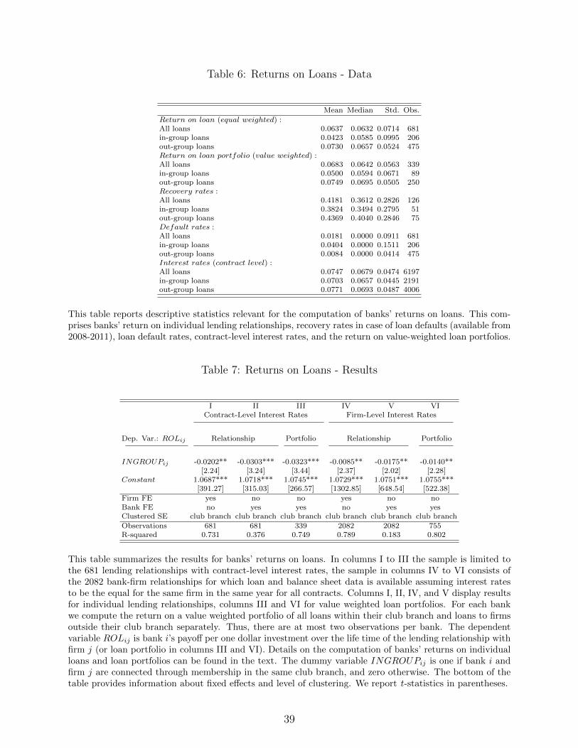
Table 6: Returns on Loans - Data

Mean Median Std. Obs.

Return on loan (equal weighted) :All loans 0.0637 0.0632 0.0714 681in-group loans 0.0423 0.0585 0.0995 206out-group loans 0.0730 0.0657 0.0524 475Return on loan portfolio (value weighted) :All loans 0.0683 0.0642 0.0563 339in-group loans 0.0500 0.0594 0.0671 89out-group loans 0.0749 0.0695 0.0505 250Recovery rates :All loans 0.4181 0.3612 0.2826 126in-group loans 0.3824 0.3494 0.2795 51out-group loans 0.4369 0.4040 0.2846 75Default rates :All loans 0.0181 0.0000 0.0911 681in-group loans 0.0404 0.0000 0.1511 206out-group loans 0.0084 0.0000 0.0414 475Interest rates (contract level) :All loans 0.0747 0.0679 0.0474 6197in-group loans 0.0703 0.0657 0.0445 2191out-group loans 0.0771 0.0693 0.0487 4006

This table reports descriptive statistics relevant for the computation of banks’ returns on loans. This com-prises banks’ return on individual lending relationships, recovery rates in case of loan defaults (available from2008-2011), loan default rates, contract-level interest rates, and the return on value-weighted loan portfolios.

Table 7: Returns on Loans - Results

I II III IV V VIContract-Level Interest Rates Firm-Level Interest Rates

Dep. Var.: ROLij Relationship Portfolio Relationship Portfolio

INGROUPij -0.0202** -0.0303*** -0.0323*** -0.0085** -0.0175** -0.0140**[2.24] [3.24] [3.44] [2.37] [2.02] [2.28]

Constant 1.0687*** 1.0718*** 1.0745*** 1.0729*** 1.0751*** 1.0755***[391.27] [315.03] [266.57] [1302.85] [648.54] [522.38]

Firm FE yes no no yes no noBank FE no yes yes no yes yesClustered SE club branch club branch club branch club branch club branch club branch

Observations 681 681 339 2082 2082 755R-squared 0.731 0.376 0.749 0.789 0.183 0.802

This table summarizes the results for banks’ returns on loans. In columns I to III the sample is limited tothe 681 lending relationships with contract-level interest rates, the sample in columns IV to VI consists ofthe 2082 bank-firm relationships for which loan and balance sheet data is available assuming interest ratesto be the equal for the same firm in the same year for all contracts. Columns I, II, IV, and V display resultsfor individual lending relationships, columns III and VI for value weighted loan portfolios. For each bankwe compute the return on a value weighted portfolio of all loans within their club branch and loans to firmsoutside their club branch separately. Thus, there are at most two observations per bank. The dependentvariable ROLij is bank i’s payoff per one dollar investment over the life time of the lending relationship withfirm j (or loan portfolio in columns III and VI). Details on the computation of banks’ returns on individualloans and loan portfolios can be found in the text. The dummy variable INGROUPij is one if bank i andfirm j are connected through membership in the same club branch, and zero otherwise. The bottom of thetable provides information about fixed effects and level of clustering. We report t-statistics in parentheses.

39

Tab

le8:

Ret

urn

son

Loa

ns

arou

nd

Eve

nts

III

III

IVV

VI

VII

VII

IIX

Entr

yF

orm

ati

on

May

ora

lE

lect

ion

Dep

.va

r.:ROLij

Rel

atio

nsh

ipP

ort

foli

oR

elati

on

ship

Port

folio

Rel

ati

on

ship

Port

folio

AFTER

jt

-0.0

068

-0.0

123

-0.0

187*

0.0

086

0.0

004

-0.0

107

-0.0

047

-0.0

049

0.0

001

[1.0

8][1

.52]

[1.9

7]

[0.7

7]

[0.0

3]

[0.6

9]

[0.6

3]

[0.4

6]

[0.0

0]

INGROUPij

-0.0

006

-0.0

159

-0.0

06

-0.0

045

0.0

147

0.0

053

0.0

127

0.0

129

-0.0

162

[0.0

6][1

.23]

[0.4

1]

[0.2

9]

[0.8

5]

[0.2

3]

[0.6

3]

[0.4

9]

[0.5

5]

AFTER

jt∗INGROUPij

-0.0

329*

**-0

.0353**

-0.0

496***

-0.0

393***

-0.0

475**

-0.0

613*

*-0

.0956***

-0.0

921***

-0.0

672**

[2.8

8][2

.46]

[2.9

5]

[2.2

7]

[2.6

2]

[2.4

5]

[4.6

3]

[3.1

0]

[2.2

5]

Constant

1.07

25**

*1.

0810***

1.0

892***

1.0

784***

1.0

673***

1.0

814*

**

1.0

678***

1.0

674***

1.0

689***

195.

1215

4.3

6137.6

9108.7

798.9

778.8

2216.2

4156.8

0144.5

6F

ixed

Eff

ects

firm

ban

kb

an

kfirm

ban

kb

an

kfi

rmb

an

kb

an

kC

lust

ered

SE

clu

bb

ran

chcl

ub

bra

nch

clu

bb

ran

chcl

ub

bra

nch

clu

bb

ran

chcl

ub

bra

nch

clu

bb

ran

chcl

ub

bra

nch

clu

bb

ran

chO

bse

rvat

ion

s41

141

1304

174

174

141

232

232

130

R-s

qu

ared

0.73

60.

623

0.6

72

0.6

68

0.7

08

0.7

100.7

22

0.5

42

0.7

17

Th

ista

ble

sum

mar

izes

the

resu

lts

for

ban

ks’

retu

rns

on

loan

sfo

rw

hic

hit

isp

oss

ible

toex

tract

contr

act

-lev

elin

tere

stra

tes

(see

Ap

pen

dix

C)

for

firm

sth

atar

eaff

ecte

dby

the

resp

ecti

ve

even

tsp

ecifi

edat

the

top

of

the

tab

le(e

ntr

y,fo

rmati

on

s,m

ayora

lel

ecti

on

s).

For

each

firm

-ban

kp

air

we

spli

tth

elo

an

sin

two

grou

ps:

thos

eor

igin

ated

bef

ore

the

even

tan

dth

ose

ori

gin

ate

daft

erth

eev

ent

an

dco

mp

ute

the

retu

rnp

eron

ed

oll

ar

inve

stm

ent

sep

ara

tely

for

bot

hgr

oup

s.C

olu

mn

sI,

II,

IV,

V,

VII

,an

dV

III

dis

pla

yth

ere

sult

sfo

rin

div

idu

al

len

din

gre

lati

on

ship

s,co

lum

ns

III,

VI,

an

dIX

for

valu

ew

eighte

dlo

an

por

tfol

ios.

For

the

por

tfol

iote

sts

we

com

pu

teth

ere

turn

on

ava

lue

wei

ghte

dp

ort

folio

of

all

loan

sw

ith

inth

eir

clu

bb

ran

chan

dlo

an

sto

firm

sfr

om

ou

tsid

eth

eir

clu

bb

ran

chse

par

atel

yfo

rea

chbank.

Thu

s,th

ere

are

at

most

two

ob

serv

ati

on

sp

erb

an

k.

Th

ed

epen

den

tva

riab

leROLij

isb

an

ki’

sp

ayoff

per

one

dol

lar

inve

stm

ent

over

the

life

tim

eof

the

len

din

gre

lati

on

ship

wit

hfi

rmj

(or

the

loan

port

foli

oin

colu

mn

sII

Ian

dV

I).

Det

ail

edex

pla

nati

on

of

the

com

pu

tati

onof

ban

ks’

retu

rns

onin

div

idual

loan

san

dlo

an

port

foli

os

can

be

fou

nd

inth

ete

xt.

Th

ed

um

my

vari

ab

leINGROUPij

ison

eif

banki

an

dfi

rmj

are

con

nec

ted

thro

ugh

mem

ber

ship

inth

esa

me

clu

b,

an

dze

rooth

erw

ise.

Inco

lum

ns

VII

toIX

the

’in

-gro

up

’b

an

kis

the

loca

lst

ate

ban

kin

wh

ich

the

new

lyel

ecte

dm

ayor

bec

omes

hea

dof

the

sup

ervis

ory

board

thro

ugh

her

elec

tion

.T

he

bott

om

of

the

tab

lep

rovid

esin

form

ati

on

ab

ou

tfi

xed

effec

tsan

dle

vel

ofcl

ust

erin

g.W

ere

por

tt-

stat

isti

csin

par

enth

eses

.

40

Tab

le9:

Len

din

gShar

esof

In-g

roup

Ban

ks

-B

yB

ank

Ow

ner

ship

III

III

IVV

VI

Dep

.V

ar.:

( In−group

bank

loans

Tota

lfirm

loans

) jt

( Sta

tein−group

bank

loans

Tota

lin−group

bank

loans

) jt

( In−group

bank

loans

Tota

lfirm

loans

) jt

Sta

teP

riva

teC

oop

erati

ves

On

eb

an

kM

ult

iple

ban

ks

Sta

te

AFTER

jt

0.10

82**

*0.0

763***

0.0

472

0.0

592***

0.1

426*

0.0

626**

[3.6

3][4

.66]

[1.2

8]

[4.5

6]

[1.9

4]

[2.2

0]

AFTER

jt∗STATE

k0.0

645**

[2.3

4]

AFTER

jt∗MAYOR

k0.1

283***

[2.8

9]

Qu

arte

rF

Eye

sye

sye

sye

sye

syes

Fir

mF

Eye

sye

sye

sye

syes

yes

Clu

ster

edS

Ecl

ub

bra

nch

clu

bb

ran

chcl

ub

bra

nch

club

bra

nch

clu

bb

ran

chcl

ub

bra

nch

Ob

serv

atio

ns

4214

6936

866

12016

12696

4214

R-s

qu

ared

0.51

10.4

45

0.3

63

0.4

73

0.6

62

0.5

54

For

the

dep

end

ent

vari

able

inth

ista

ble

we

div

ide

firm

j’s

loan

sfr

om

its

in-g

rou

pb

an

kby

firm

j’s

tota

llo

an

sin

colu

mn

sI

toIV

an

dV

I.T

he

sam

ple

inco

lum

ns

Ito

IVis

lim

ited

tocl

ub

bra

nch

esw

ith

on

lyon

ein

-gro

up

ban

k,

wh

ich

isei

ther

ast

ate

ban

k(c

olu

mn

I),

ap

riva

teb

an

k(c

olu

mn

II)

or

aco

oper

ativ

eb

ank

(col

um

nII

I).

Th

esa

mp

lein

colu

mn

Vco

mp

rise

sall

clu

bb

ran

ches

that

hav

etw

oin

-gro

up

ban

ks

on

eof

wh

ich

isa

state

in-g

rou

pb

an

kan

don

eof

wh

ich

isa

pri

vate

orco

oper

ativ

ein

-gro

up

ban

k.

Th

ed

epen

den

tva

riab

leis

rep

lace

dby

firm

j’s

state

in-g

rou

pb

an

klo

an

sd

ivid

edby

firm

j’s

tota

llo

ans

from

all

in-g

rou

pb

anks.

Th

eva

riab

leAFTER

jt

isa

du

mm

yva

riab

leta

kin

gth

eva

lue

of

on

efr

om

the

yea

rw

hen

firm

jen

ters

acl

ub

bra

nch

,an

dze

root

her

wis

e.T

heSTATE

kd

um

my

take

sth

eva

lue

of

on

efo

rfi

rms

ass

oci

ate

dto

acl

ub

bra

nch

wit

ha

state

ban

ker

an

dze

rofo

rfi

rms

ass

oci

ate

dw

ith

bra

nch

that

hav

en

ost

ate

ban

ker

amon

git

sm

emb

ers.

For

asu

bsa

mp

leof

bra

nch

esth

em

ayor

of

the

resp

ecti

veci

tyis

mem

ber

of

the

bra

nch

(an

dsi

mu

ltan

eou

sly

hea

din

gth

eb

oard

ofth

est

ate

ban

k).

For

those

bra

nch

esth

eMAYOR

kva

riab

leta

kes

the

valu

eof

on

e,w

her

eas

for

bra

nch

esw

ith

no

may

orit

take

sth

eva

lue

ofze

ro.

Th

esa

mp

lein

colu

mn

VI

isre

stri

cted

tob

ran

ches

inw

hic

hth

ein

-gro

up

ban

kis

ast

ate

ban

k.

Each

regre

ssio

nin

clu

des

qu

arte

ran

dfirm

fixed

effec

ts.

Sta

nd

ard

erro

rsar

eco

rrec

ted

for

clu

ster

ing

at

the

clu

bb

ran

chle

vel.

We

rep

ort

t-st

ati

stic

sin

pare

nth

eses

.

41

Table 10: Returns on Loans - By Bank Ownership

I II III IVDep. Var.: ROLip State Private Cooperatives All

INGROUPij -0.0564*** -0.0187** -0.0026 -0.0166[2.88] [2.02] [0.16] [1.40]

INGROUPij ∗ STATEi -0.0398**[2.11]

Constant 1.0680*** 1.0744*** 1.0866*** 1.0745***[111.21] [267.68] [237.13] [271.62]

Bank FE yes yes yes yesClustered SE club branch club branch club branch club branch

Observations 105 175 59 339R-squared 0.671 0.744 0.982 0.761

This table summarizes the estimation results for portfolio-level returns on loans for different bank groups.The sample comprises the firms for which contract-level interest rates can be computed (see Appendix C).We compute the return on a value-weighted portfolio separately for loans to firms within the club branchand firms in other branches. Thus for each bank there are at most two observations. The dependentvariable ROLip is bank i’s payoff per one dollar investment over the life time of portfolio p. A detailedexplanation of the computation of portfolio-level returns on loans can be found in the text. The dummyvariable INGROUPij is one if bank i and the firms in portfolio p are connected through membership in thesame club branch, and zero otherwise. The STATEi dummy takes the value of one if bank i is a state bank,and zero otherwise. All regressions include bank fixed effects. Standard errors are corrected for clusteringat the club branch level. We report t-statistics in parentheses.

Table 11: Firms’ Usage of Capital

I II III IV V VI

Dep. Var.:(

InvestmentsAssets

)jt

(CashAssets

)jt

(PayoutsAssets

)jt

(Debt

Assets

)jt

(EBITAssets

)jt

(Interest exp.

Debt

)jt

AFTERjt -0.0063 0.0271*** 0.0289*** 0.0617*** 0.0018 -0.0040[0.65] [2.71] [2.83] [2.67] [0.28] [1.33]

Year FE yes yes yes yes yes yesFirm FE yes yes yes yes yes yesClustered SE club branch club branch club branch club branch club branch club branch

Observations 4751 5474 4751 4364 5474 5094R-squared 0.402 0.698 0.379 0.762 0.558 0.404

This table depicts changes in firm-level variables for the subsample of 686 firms for which balance sheet datafrom the USTAN database is available. Information on the dependent variable of each regression is providedat the top of the table. The dummy variable AFTERjt takes the value of one from the year when firm jjoins a club branch and zero otherwise. All regressions include year and firm fixed effects. Standard errorsare corrected for clustering at the club branch level. We report t-statistics in parentheses.

42

Table 12: Lending Decisions and Future Changes in Firm Performances

Panel A: Profitability I II III IV V VI VII VIIIPopulation Sample Club Loans Outside Loans

Dep. Variable: ROAt+k −ROAt k=2 k=5 k=2 k=5 k=2 k=5 k=2 k=5∆ loansijtassetsjt

0.0255*** 0.0273*** 0.0037 0.0151*** -0.0552** -0.0323* 0.0045 0.0156***

[4.69] [3.74] [0.47] [4.51] [2.60] [1.97] [0.54] [3.54]club bankij -0.0029* -0.0005

[1.88] [0.47]∆ loansijtassetsjt

∗ club bankij -0.0588*** -0.0410***

[3.02] [2.65]Year FE yes yes yes yes yes yes yes yesFirm FE yes yes yes yes yes yes yes yesBank FE yes yes yes yes yes yes yes yesFirm Controls yes yes yes yes yes yes yes yesClustered SE firm firm firm firm firm firm firm firmObservations 71737 36848 6806 4206 2132 1305 4674 2901R-squared 0.260 0.399 0.661 0.870 0.706 0.892 0.656 0.869

Panel B: Firm Risk I II III IV V VI VII VIIIPopulation Sample Club Loans Outside Loans

Dep. Variable: PDt+k − PDt k=2 k=5 k=2 k=5 k=2 k=5 k=2 k=5∆ loansijtassetsjt

-0.1841** -0.1718* -0.1572* -0.2717** 0.1327 0.0666 -0.2121** -0.3583***

[2.41] [1.82] [1.85] [2.54] [0.20] [0.08] [2.21] [2.87]club bankij -0.0126 -0.0598

[0.57] [1.63]∆ loansijtassetsjt

∗ club bankij 0.0779 0.0721

[0.12] [0.08]Year FE yes yes yes yes yes yes yes yesFirm FE yes yes yes yes yes yes yes yesBank FE yes yes yes yes yes yes yes yesFirm Controls yes yes yes yes yes yes yes yesClustered SE firm firm firm firm firm firm firm firmObservations 69316 35551 5393 3152 1717 1001 3676 2151R-squared 0.335 0.566 0.443 0.642 0.493 0.656 0.446 0.659

The dependent variable in this table ROAjt+k − ROAjt is firm j’s average return on assets from t + 2

to t + k minus its current return on assets. The variable∆ loansijtassetsjt

is the change in loans from bank i to

firm j from t − 1 to t scaled by firm j’s assets. The dummy variable club bankij takes the value of one ifbank i is club bank in firm j’s club and zero otherwise. We only consider loans to firms when they are amember of the club, except in columns I and II, where the sample comprises all firms in the sample regionnot associated to the social club organization. In columns V and VI the sample comprises only within clubloans, in columns VII and VIII the sample is limited to loans from banks that are member of a differentclub branch than the firm. We include year, firm and bank fixed effects in every regression. As firm controlswe add the logarithm of lagged firm assets, and industry trends*. T-statistics are reported in parantheses.Standard errors are corrected for clustering at the firm level.

43

Figure 1: Service Club Membership in Germany

0

10,000

20,000

30,000

40,000

50,000

60,000

70,000

80,000

90,000

100,000

1990 1991 1992 1993 1994 1995 1996 1997 1998 1999 2000 2001 2002 2003 2004 2005 2006 2007 2008 2009 2010 2011 2012

Year

Se

rvic

e C

lub

Me

mb

ers

This figure depicts the time-series evolution of aggregate membership to the two largest service clubs inGermany.

Figure 2: In-group Bank Share in Total Firm Lending Around Entry to a Branch

0.1

0.12

0.14

0.16

0.18

0.2

0.22

0.24

0.26

-5 -4 -3 -2 -1 0 1 2 3 4 5

Years before/after entrance

In-g

rou

p B

an

k/T

ota

l Lo

an

s

This figure depicts the share of loans from a firm’s in-group bank divided by the firm’s total loans for thesample of 474 firms that enter a branch during the sample period. To compute the in-group bank shares onthe y-axis we align firms around the year they enter a branch and calculate the average in-group bank sharefor all firms with the same distance to entry. The x-axis displays the distance to firms’ entry to a branch inyears. The value zero indicates the year in which the firm officially obtains member status in the branch.

44

Figure 3: State Bank Share in Total Firm Lending Around Mayoral Elections

0.16

0.18

0.2

0.22

0.24

0.26

0.28

0.3

-5 -4 -3 -2 -1 0 1 2 3 4 5

Years before/after entrance

In-g

rou

p B

an

k/T

ota

l Lo

an

s

This figure depicts the share of loans a firm borrows from the state bank divided by its total loans for thesample of 109 firms that are members of a club branch in which an existing member in elected as a mayorfor the first time during the sample period and thereby becomes head of the local state bank’s supervisoryboard. To compute the state bank shares on the y-axis we align firms around the year of the mayoral electionand calculate the average state bank share for all firms with the same distance to the mayoral election.

45

Figure 4: Bank Lending Shares before Bankruptcy

-0.04

-0.02

0

0.02

0.04

0.06

0.08

0.1

0.12

0.14

-16 -15 -14 -13 -12 -11 -10 -9 -8 -7 -6 -5 -4 -3 -2 -1 0

All In-group Banks Main Lender In-group Banks Main Lender Population

-0.04

-0.02

0

0.02

0.04

0.06

0.08

0.1

0.12

0.14

0.16

0.18

0.2

-16 -15 -14 -13 -12 -11 -10 -9 -8 -7 -6 -5 -4 -3 -2 -1 0

Private In-group Banks State In-group Banks

Quarters to bankruptcy

Quarters to bankruptcy

In-g

rou

p B

an

k/T

ota

l Lo

an

sIn

-gro

up

Ba

nk

/To

tal L

oa

ns

Panel A of this figure plots the share of in-group bank in total firm loans in the sixteen quarters before firms’default on the y-axis (solid lines). We plot in-group bank shares relative to the share sixteen quarters beforebankruptcy which we set to zero. The x-axis lists the distance to the official bankruptcy date in quarters.The gray solid line comprises all firms with a default event in the sample, whereas the black solid line onlyincludes those firms for which additionally the in-group bank is their main lender. The gray dashed linedepicts the share of loans from firms’ main lender in total firm loans for the population of all firms in thesample region that are not club members (and therefore not part of our sample). Panel B plots the share ofin-group bank in total firm loans for the firms with a default event whose in-group bank is the main lenderseparately for firms for which the in-group bank is a state bank (black line) and for firms for which thein-group bank is a private bank (gray line).

46

Appendix A. Data collection of service club members

This appendix describes the construction of the dataset on service club members. Many of

these service club branches provide their entire membership section through their website.

Other service club branches only provide the names of current members and the official

function within the branch (e.g. president, vice-president, treasury), as well as the names of

members that had an official function in the past. Since the branches tend to be small (on

average 50 members) and we are only interested in members that are either a firm’s CEO

or a bank director, we obtain most member names by this search strategy. We complete our

sample by interviewing club members from our sample region.

Membership information includes an entrance date, as well as information on the mem-

ber’s profession. If the information regarding a member’s profession is incomplete, we update

our sample by internet research. Names of CEOs of limited liability and public firms can be

obtained through the federal German corporate register (elektronischer Bundesanzeiger).45

We also use the latter source to identify whether the firms in the service clubs filed for

bankruptcy during our sample period. All sample banks list their regional directors on each

bank’s website.

Appendix B. The German banking sector

The German financial sector is bank-based with a universal banking system. The German

banking sector consists of 2,277 banks and nearly 40,000 bank branches.46 One of the

distinct features of the German banking sector is the so-called three-pillar structure which

refers to the three different types of legal ownership of German banks - state owned banks

(Landesbanken and Sparkassen), private banks, and credit cooperatives. The market shares

of these different types of banks according to banking assets are distributed as follows: 39

percent are held by private banks, 45.5 percent by state banks (that break down in 25 percent

by savings banks (Sparkassen), and 20.5 by Landesbanken), and 15.5 percent by cooperative

banks. While savings banks and cooperative banks share a regional structure, private banks

tend to have one headquarter (mostly in Frankfurt) and operate bank branches throughout

Germany. An illustration of the most important institutional features of these three different

types of banks is provided in Table A.1.

45https://www.ebundesanzeiger.de46Within Europe, Germany is among the countries with the highest number of credit institutions, branches,

and bank employees; see ECB (2007) for details.

47

Table A.1: Banks in Germany

Private Banks State-Owned Banks (excl.Landesbanken)

Cooperative Banks

Ownership shareholders local government customers are shareholders(members)

Geographic Outreach national regional (local) regional (local)

Liability limited liability of shareholders public guarantee obligation un-til 2005; implicit public guar-antee through state ownership

liability of members (if lossesexceed equity, members haveto inject new capital)

Deposit Insurance private fund to secured the de-posits of customer up to a ceil-ing of 30 percent of the liablecapital of each bank

federal association of stateowned banks to support en-tire bank (not just deposits);capital injections from regionalgovernment

federal association provides aninsurance fund to provide de-posit guarantees

Market Share 39 percent 25 percent 15.5 percent

This table provides information about the organizational structure of the three groups of German banks:private banks, state-owned banks (savings banks, excl. Landesbanken), and cooperatives. It depicts infor-mation on ownership of the banks, their geographic outreach, owners’ liability, deposit insurance, and theirrespective market share according to banking assets.

The structure of the state banking sector is the result of laws (Sparkassengesetz ) imple-

mented at the beginning of the twentieth century and after the Second World War, which

gave rise to a country-wide community savings banking sector. Savings banks are owned and

controlled by the local politicians exercise governance through the supervisory board of the

savings banks. Furthermore, local politicians are members of a so called credit committee

(Kreditausschuss) that has to approve lending decisions on large loans of the savings banks.

Thus, local politicians have a direct influence on the state banks management decisions. The

regional principle requires savings banks to foster credit supply in the city/county of their

location. The objectives of state banks, as laid down in the respective laws (e.g., SpGNRW

and SpGBW ), are besides generating income to the local government manifold: e.g., ensur-

ing the availability of credit to enterprises and communities, as well as facilitating individual

savings.47 Since regional state-owned banks are owned and controlled by the local politicians,

these politicians may use taxpayers money to support these banks in case of distress.

German cooperative banks are organized in a very similar way as state-owned banks.

They have the same regional organization but operate independent of the local government.

Thus, the main difference between these two types of banks is their ownership structure.

47Commonly this legal framework includes a statement that profit maximization is not the only objectiveof state owned banks. Other objectives are to provide a checking account to every private person independentof her income and the economic education of the youth (see the Sparkassengesetze, Sparkassenordnung andLandesbankgesetz of the Lander in German.

48

While savings banks are owned by the government, cooperative banks are owned by private

shareholders (i.e., referred to as members). According to the institutional set-up of cooper-

atives, only customers of the bank may become shareholders of the banks. Furthermore, in

case a bank encounters losses that are higher than its equity, shareholders are required to

inject further capital (no limited liability). Thus, the governance of cooperative and private

banks is basically very similar since both types of banks are controlled for by shareholders

that benefit from higher bank profits. Savings banks, however, are controlled by the local

politicians. In this case, the budget of the city/county would benefit from high profits by the

savings bank, while there is no direct benefit for the politician. We exploit this difference

in governance that is very likely to be stricter for private and cooperatives as opposed to

state-owned banks. For further details see Engelmaier and Stowasser (2013).

Appendix C. Computation of Interest Rates

Combining the quarterly Bundesbank credit register with annual firm-level accounting in-

formation from USTAN allows us to back out effective annual interest rates on the loan

contract level.

Step 1: As a first step, we use quarterly information from the credit register on the bank-

firm relationship level to identify individual loan contracts. From the repayment structure

of the initial loan amount, we can infer the maturity of the loan contract (e.g., whether it

is repaid at the end of the contract period; linearly or de/progressively). If the outstanding

loan of a lending relationship increases, we identify a new loan contract. Some lending

relationships include a current account for the client with a loan amount that fluctuates

around a fairly stable mean. Therefore, we only identify a new loan contract if the increase

in total loans per firm-bank relationship exceeds 33.33 percentage points. Following this

procedure, we extract all individual loan contracts per firm from the credit register (see

Table A.2, Panel A).48

48The tables in this section help to guide the reader through the computation of interest rates by illustratingone hypothetical example.

49

Table A.2: Contract Extraction

A - Quarterly Data I II III IV VQuarter Bank A Bank B Contract 1 (A) Contract 2 (A) Contract 3 (B)1998 Q4 12000 - 12000 - -1999 Q1 10000 - 10000 - -1999 Q2 8000 - 8000 - -1999 Q3 6000 - 6000 - -1999 Q4 11000 - 4000 7000 -2000 Q1 9000 - 2000 7000 -2000 Q2 7000 - - 7000 -2000 Q3 7000 - - 7000 -2000 Q4 7000 - - 7000 -2001 Q1 7000 - - 7000 -2001 Q2 7000 - - 7000 -2001 Q3 7000 5000 - 7000 50002001 Q4 - 4000 - - 40002002 Q1 - 3000 - - 30002002 Q2 - 2000 - - 20002002 Q3 - 1000 - - 1000

B - Annualized Data I II III IV VYear IR Spread Contract 1 (A) Contract 2 (A) Contract 3 (B)1999 0.0700 0.0381 9000 - -2000 0.0853 0.0367 1500 7000 -2001 0.0803 0.0399 - 7000 12502002 0.0800 0.0451 - - 2500

Panel A of this table lists a firm’s total loans from Bank A in column I and Bank B in column II derived fromthe credit register. Columns III to V display the contracts extracted from the quarterly loan information.Panel B depicts the annualized data. Column I shows the annual firm-level interest rate from balance sheetdata, column II the spread of the interest rate over the EURIBOR. Columns III to V lists the average annualloan for Contracts 1 to 3. Details on the identification of loan contracts can be found in the text.

To match loan and balance sheet data, we annualize the loan data by averaging the loan

amount over four quarters (Decembert−1, Marcht, Junet, Septembert). We match contract-

level information with interest payments derived from balance sheet information49 (see Ta-

ble A.2, Panel B). In rare cases, firms have interest-relevant debt in excess of bank loans. In

this case, the sum of all bank loans from the credit register does not sum up to the amount

of loans reported in a firm’s balance sheet. We deal with this discrepancy by treating the

difference as an additional lending relationship.

Step 2: The combination of both datasets allows us to compute contract-level interest

rates by solving the equation system:

rjt =D∑d=1

xdjt∑Dd=1 xdjt

· rdj, (C.1)

for t = t− int(D/2), ..., t, ..., t+ int((D − 1)/2)

49Annual firm-level interest rates are defined as interest expenses minus interest expenses to related firms(ap174-ap175) divided by the average loan amount in the same year.

50

where D is the number of relationships. The variable rjt is the average interest rate paid

by firm j in year t. We winsorize firm-level interest rates at the 5/95 percent quintile to

account for unduly extreme outliers. The individual contract volume for firm j’s contracts

is denoted by xdjt, and thus,xdjt∑D

d=1 xdjtis contract d’s share in firm j’s total borrowing. The

variable of interest is rdj, the interest rate on the individual loan contract.50

Each contract can either be a fixed or floating rate contract.51 Equation system (C.1)

can also be solved for floating rate contracts by replacing rdj by (sdj +EURIBORt), where

sdj is the spread over the EURIBOR for contract d. As we do not have information about

the type of contract, we allow all possible combinations for each firm at every point in time.

For a firm with D contracts at a given point in time, we solve 2D different equation systems.

Additionally, for D contracts to solve the equation system for rdj, D independent equa-

tions are required. Solving the equation system provides us with contract-specific interest

rates/spreads (see Table A.3).

Step 3: To identify the correct combination of contract types, we first calculate the average

absolute deviation from the mean interest rate/spread for each contract:

σdjt =1

T·

T∑t=1

∣∣∣rdjt −∑T

t=1

rdjtT

∣∣∣ (C.2)

where T is the maturity of contract d in years. Next, we compute the average deviation for

each of the 2D equation systems as the average deviation over all contracts as ςj. For each

firm, we pick the combination of fixed and floating rate contracts that leads to the lowest

value of ςj (see Table A.3). Finally, we calculate the annual firm-bank relationship level

interest rate as the value-weighted interest rate of all contracts of a firm-bank relationship

for a given year. This approach allows us to compute firm-bank level interest rates for a

subsample of lending relationships for which equation system (C.1) is solvable.

Step 4: To verify the validity of the computed interest rates we run within sample plausi-

bility tests and apply the algororith to a sample of contracts for which we collect information

on actual interest rates. From 2008, for every loan the credit register provides information

about whether a loan is secured or unsecured, and the lender’s reported probability of de-

fault. Within sample tests allow us comparing interest rates of the same firm in the same

year, which is insightful as differences in interest rates for the same firm in the same year

50In the example from Table A.2, the equation system for the year 2000 with fixed interest rates is:[0.08530.0803

]=

[1 0

0.1765 0.8235

]×[r1

r2

].

51In Germany, floating rate contracts use the FIBOR as base rate until 1998 and the EURIBOR as of1999.

51

Table A.3: Solutions

(r,r,r) (s,s,s) (r,s,s) (r,r,s) (r,s,r) (s,r,r) (s,r,s) (s,s,r)1999Contract 1 (A) 0.0700 0.0381 0.0700 0.0700 0.0700 0.0381 0.0381 0.0381Contract 2 (A) - - - - - - - -Contract 3 (B) - - - - - - - -2000Contract 1 (A) 0.0700 0.0381 0.0700 0.0700 0.0700 0.0381 0.0381 0.0381Contract 2 (A) 0.0886 0.0364 0.0400 0.0886 0.0400 0.0850 0.0850 0.0364Contract 3 (B) - - - - - - - -2001Contract 1 (A) 0.0700 0.0381 0.0700 0.0700 0.0700 0.0381 0.0381 0.0381Contract 2 (A) 0.0886 0.0364 0.0400 0.0886 0.0400 0.0850 0.0850 0.0364Contract 3 (B) 0.0339 0.0595 0.0395 -0.0065 0.0799 0.0540 0.0136 0.09992002Contract 1 (A) - - - - - - - -Contract 2 (A) 0.0804 0.0390 0.0390 0.0794 0.0400 0.0804 0.0794 0.0462Contract 3 (B) 0.0800 0.0451 0.0451 0.0451 0.0800 0.0800 0.0451 0.0451

σ(Contract 1 (A)) 0.0000 0.0000 0.0000 0.0000 0.0000 0.0000 0.0000 0.0000σ(Contract 2 (A)) 0.0101 0.0031 0.0012 0.0113 0.0000 0.0057 0.0069 0.0120σ(Contract 3 (B)) 0.0345 0.0108 0.0042 0.0387 0.0001 0.0195 0.0236 0.0411

ς 0.0149 0.0046 0.0018 0.0166 0.0000 0.0084 0.0102 0.0177

The first line of the table indicates the combination of fixed rate contracts (r) and floating rate contracts (s).The optimal combination of contracts to solve the equation system is (r,s,r). The interest rate for Contract 1is 0.08, the spread for Contract 2 is 0.04, and the interest rate for Contract 3 is 0.07. This leads to annualinterest rates of 0.0700 in 1999, 0.0853 in 2000, and 0.0804 in 2001 for Bank A, and 0.0800 in 2001 and 2002for Bank B.

52

Table A.4: Within-Sample Plausibility Tests

Secured vs. unsecured Firm risk

Dep. Var.: IRijt I II III IV V VIsecuredijt -0.0052* -0.0104*** -0.0175***

[1.88] [3.33] [3.56]log(PD)ijt 0.0020* 0.0049*** 0.0075**

[1.77] [2.74] [2.23]Year FE yes yes - yes yes -Firm FE no yes - no yes -Firm-Year FE no no yes no no yesObservations 1093 1093 1093 636 636 636R-squared 0.052 0.571 0.652 0.063 0.621 0.731

This table shows the results from the regression: IRijt = α+ β · securedijt + εijt in columns I to III, whereIRijt is the relationship-level interest rate charged by bank i for firm j at time t and securedijt is a dummyvariable taking the value of one if the loan is secured and zero otherwise. In columns IV to VI the securedijtdummy is replaced by log(PD)ijt, the log of the probability of default assigned from bank i to firm j at timet. The bottom part of the table lists the fixed effects included. We report t-statistics in parentheses.

emerge solely from the algorithm to computate relationship-level interest rates. In the cross-

section, interest rates on secured loans are 0.52 percentage points lower than for unsecured

loans (Table A.4, column I). After adding firm fixed effects, the difference is even larger, with

1.04 percentage points (column II). With firm-year fixed effects, interest rates on secured

loans are are 1.75 percent lower than for unsecured loans (column III). Additionally, interest

rates are higher for riskier firms (column IV). After adding firm fixed effects, the difference

is even stronger (column V). Adding firm-year fixed effects reveals that banks that consider

the same firm to be riskier (that is, report a higher probability of default) charge higher

interest rates (column VI). The results from the plausibility checks verify that the computed

interest rates capture differences in interest rates across loan contracts correctly. In partic-

ular, the algorithm to compute relationship level interest rates improves the cross-sectional

distribution of interest rates suggesting that it captures differences in interest rates well.

We obtain actual interest rates from the Center for Financial Studies (CFS) Loan Data

Set used in Brunner and Krahnen (2008, 2013).52 The dataset comprises, for a randomly

drawn set of medium-sized firms, bank-borrower relationship level interest rates collected

from five major banks (three private banks, one public sector bank, and one cooperative

bank) from 1992 to 1996. We additionally update the data for the 2011-2012 period for one

bank. In total we can match 93 of the firms with balance sheet and loan data at Bundesbank.

For 87 out of the 93 firms balance sheet and loan data overlaps (is available for the same

52We thank Jan-Pieter Krahnen for providing us with the data.

53

year), allowing us to estimate interest rates. For 72 of the firms such information is available

in at least one year for which we obtained actual interest rates. We start with 164 firm-year

observations for which real and balance sheet level interest rates are available. For 167 of the

725 annual firm-bank relationships that exist for those 164 firm-year observations, we know

the actual interest rate. After applying the algorithm we obtain 100 estimated relationship-

level interest rates for 50 firms. Since Bundesbank rules require each reported data point

to comprise at least three individual observations, we summarize three adjacent estimated

interest rates into 33 buckets (the last bucket contains four observations) for the graphical

analysis. Figure A.1 plots the average actual interest rates against the average estimated

interest rates for those 33 buckets including a 45 degree line. The correlation between the

actual and estimated interest rates is 0.9429. When we regress the actual interest rate on

estimated interest rates, the slope is close to one with 1.0574 (Table A.5, column I). When

we add a constant to the regression the constant term is insignificant with 0.44 percentage

points, the slope coefficient is 0.9929 (column II). The comparison with actual interest rates

shows that the algoritmn to compute relationship-level interest rates provides a reasonable

proxy for actual interest rates.

Figure A.1: Actual and Estimated Interest Rate

0

0.02

0.04

0.06

0.08

0.1

0.12

0 0.02 0.04 0.06 0.08 0.1 0.12

IR estimated

IR r

ea

l

This figure plots actual interest rates (y-axis) against estimated interest rates (x-axis) around a 45 degreeline. Individual firm-bank relationship observations are aggregated into buckets comprising three individualobservations to comply with Bundesbank reporting regulations. The plot shows the average actual interestrates and average estimated interest rates for the 33 buckets.

54

Table A.5: Actual and Estimated Interest Rate

I IIDep. Var.: IR realijt

IR estimatedijt 1.0574*** 0.9929***[56.38] [15.19]

Constant 0.0044[1.03]

Observations 100 100R-squared 0.970 0.702

This table shows the results from regressing actual firm-bank relationship interest rates (IR realijt) onestimated interest rates (IR estimatedijt) without a constant in column I and with a constant in column II.We report t-statistics in parentheses.

55