Ojo Libro Dynamica

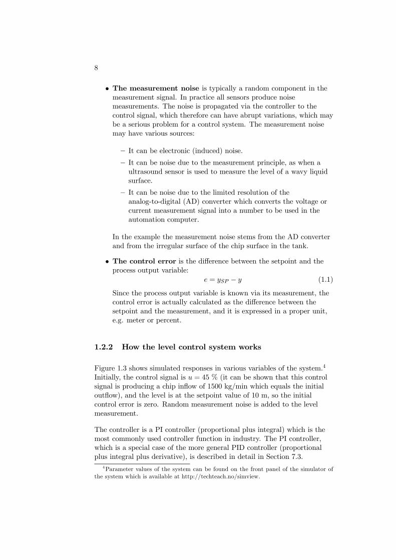
Finn Haugen

Basic DYNAMICS

and CONTROL

TechTeach techteach.no

August 2012

150 NOK (techteach.no/shop)

BasicDYNAMICS and CONTROL

Finn HaugenTechTeach

August 2010ISBN 978-82-91748-13-9

Contents

1 Introduction to control 1

1.1 The principle of error-driven control, or feedback control . . . 1

1.2 A case study: Level control of wood-chip tank . . . . . . . . . 4

1.2.1 Description of the control system with P&I diagramand block diagram . . . . . . . . . . . . . . . . . . . . 4

1.2.2 How the level control system works . . . . . . . . . . . 8

1.3 The importance of control . . . . . . . . . . . . . . . . . . . . 10

1.4 Some things to think about . . . . . . . . . . . . . . . . . . . 13

1.5 About the contents and organization of this book . . . . . . . 16

I PROCESS MODELS AND DYNAMICS 19

2 Representation of differential equations with block diagramsand state-space models 21

2.1 Introduction . . . . . . . . . . . . . . . . . . . . . . . . . . . . 21

2.2 What is a dynamic system? . . . . . . . . . . . . . . . . . . . 22

2.3 Mathematical block diagrams . . . . . . . . . . . . . . . . . . 23

2.3.1 Commonly used blocks in block diagrams . . . . . . . 23

2.3.2 How to draw a block diagram . . . . . . . . . . . . . . 24

3

4

2.3.3 Simulators based on block diagram models . . . . . . 26

2.4 State-space models . . . . . . . . . . . . . . . . . . . . . . . . 28

2.5 How to calculate static responses . . . . . . . . . . . . . . . . 31

3 Mathematical modeling 33

3.1 Introduction . . . . . . . . . . . . . . . . . . . . . . . . . . . . 33

3.2 A procedure for mathematical modeling . . . . . . . . . . . . 34

3.3 Mathematical modeling of material systems . . . . . . . . . . 36

3.4 Mathematical modeling of thermal systems . . . . . . . . . . 41

3.5 Mathematical modeling of motion systems . . . . . . . . . . . 45

3.5.1 Systems with linear motion . . . . . . . . . . . . . . . 45

3.5.2 Systems with rotational motion . . . . . . . . . . . . . 46

3.6 Mathematical modeling of electrical systems . . . . . . . . . . 49

4 The Laplace transform 55

4.1 Introduction . . . . . . . . . . . . . . . . . . . . . . . . . . . . 55

4.2 Definition of the Laplace transform . . . . . . . . . . . . . . . 55

4.3 Laplace transform pairs . . . . . . . . . . . . . . . . . . . . . 57

4.4 Laplace transform properties . . . . . . . . . . . . . . . . . . 58

5 Transfer functions 61

5.1 Introduction . . . . . . . . . . . . . . . . . . . . . . . . . . . . 61

5.2 Definition of the transfer function . . . . . . . . . . . . . . . . 62

5.3 Characteristics of transfer functions . . . . . . . . . . . . . . 64

5.4 Combining transfer functions blocks in block diagrams . . . . 65

5.5 How to calculate responses from transfer function models . . 65

5

5.6 Static transfer function and static response . . . . . . . . . . 67

6 Dynamic characteristics 69

6.1 Introduction . . . . . . . . . . . . . . . . . . . . . . . . . . . . 69

6.2 Integrators . . . . . . . . . . . . . . . . . . . . . . . . . . . . 69

6.3 Time-constant systems . . . . . . . . . . . . . . . . . . . . . . 71

6.4 Time-delays . . . . . . . . . . . . . . . . . . . . . . . . . . . . 75

6.5 Higher order systems . . . . . . . . . . . . . . . . . . . . . . . 75

II FEEDBACK AND FEEDFORWARD CONTROL 79

7 Feedback control 81

7.1 Introduction . . . . . . . . . . . . . . . . . . . . . . . . . . . . 81

7.2 Function blocks in the control loop . . . . . . . . . . . . . . . 81

7.2.1 Automatic and manual mode . . . . . . . . . . . . . . 81

7.2.2 Measurement lowpass (smoothing) filter . . . . . . . . 82

7.2.3 Scaling with percentage values . . . . . . . . . . . . . 84

7.2.4 Scaling with physical (engineering) values . . . . . . . 87

7.3 The PID controller . . . . . . . . . . . . . . . . . . . . . . . . 89

7.3.1 The ideal PID controller function . . . . . . . . . . . . 89

7.3.2 How the PID controller works . . . . . . . . . . . . . . 90

7.3.3 Positive or negative controller gain? Or: Reverse ordirect action? . . . . . . . . . . . . . . . . . . . . . . . 94

7.4 Practical modifications of the ideal PID controller . . . . . . 96

7.4.1 Lowpass filter in the D-term . . . . . . . . . . . . . . . 96

7.4.2 Reducing P-kick and D-kick caused by setpoint changes 97

6

7.4.3 Integrator anti wind-up . . . . . . . . . . . . . . . . . 98

7.4.4 Bumpless transfer between manual/auto mode . . . . 102

7.5 Control loop stability . . . . . . . . . . . . . . . . . . . . . . . 102

8 Feedforward control 105

8.1 Introduction . . . . . . . . . . . . . . . . . . . . . . . . . . . . 105

8.2 Designing feedforward control from differential equation models107

8.3 Designing feedforward control from experimental data . . . . 111

9 Controller equipment 117

9.1 Process controllers . . . . . . . . . . . . . . . . . . . . . . . . 117

9.2 Programmable logical controller (PLC) . . . . . . . . . . . . . 121

9.3 Programmable Automation Controller (PAC) . . . . . . . . . 123

9.4 SCADA systems . . . . . . . . . . . . . . . . . . . . . . . . . 123

9.5 DCS systems . . . . . . . . . . . . . . . . . . . . . . . . . . . 125

9.6 Embedded controllers in motors etc. . . . . . . . . . . . . . . 126

10 Tuning of PID controllers 129

10.1 Introduction . . . . . . . . . . . . . . . . . . . . . . . . . . . . 129

10.2 The Good Gain method . . . . . . . . . . . . . . . . . . . . . 130

10.3 Skogestad’s PID tuning method . . . . . . . . . . . . . . . . . 135

10.3.1 The background of Skogestad’s method . . . . . . . . 135

10.3.2 The tuning formulas in Skogestad’s method . . . . . . 137

10.3.3 How to find model parameters from experiments . . . 140

10.3.4 Transformation from serial to parallel PID settings . . 141

10.3.5 When the process has no time-delay . . . . . . . . . . 141

7

10.4 Auto-tuning . . . . . . . . . . . . . . . . . . . . . . . . . . . . 142

10.5 PID tuning when process dynamics varies . . . . . . . . . . . 144

10.5.1 Introduction . . . . . . . . . . . . . . . . . . . . . . . 144

10.5.2 PID parameter adjustment with Skogestad’s method . 146

10.5.3 Gain scheduling of PID parameters . . . . . . . . . . . 147

10.5.4 Adaptive controller . . . . . . . . . . . . . . . . . . . . 153

11 Various control methods and control structures 157

11.1 Cascade control . . . . . . . . . . . . . . . . . . . . . . . . . . 157

11.1.1 The principle of cascade control . . . . . . . . . . . . . 157

11.1.2 Benefits of cascade control . . . . . . . . . . . . . . . . 158

11.1.3 Controller selection and controller tuning . . . . . . . 160

11.1.4 Cascade control and state feedback . . . . . . . . . . . 161

11.2 Ratio control . . . . . . . . . . . . . . . . . . . . . . . . . . . 168

11.3 Split-range control . . . . . . . . . . . . . . . . . . . . . . . . 169

11.4 Flow smoothing with sluggish level control . . . . . . . . . . . 171

11.4.1 The control task . . . . . . . . . . . . . . . . . . . . . 171

11.4.2 Controller tuning . . . . . . . . . . . . . . . . . . . . . 172

11.5 Plantwide control . . . . . . . . . . . . . . . . . . . . . . . . . 176

12 Sequential control 185

A Codes and symbols used in Process & Instrumentation Di-agrams 191

A.1 Letter codes . . . . . . . . . . . . . . . . . . . . . . . . . . . . 191

A.2 Instrumentation symbols used in P&IDs . . . . . . . . . . . . 191

Preface

This book is about on automatic control using the industry-standard PIDcontroller, and control structures based on the PID controller.1

This book is based on a mathematical description — mathematical models —of the processes to be controlled. Models are very useful for several reasons:

• To represent processes, and other components of control systems, ina clear, conceptual way.

• To create simulators. Simulation is very convenient for design andtesting of processes and control systems.

• To characterize the dynamic properties of processes.

• To tune a PID feedback controller from the process model, as withSkogestad’s tuning method.

• To design a feedforward controller.

Despite the use of models as mentioned above, this book does not containtheoretical analysis of stability and dynamics of control systems. Also,frequency response analysis is omitted. After many years of teaching basicdynamics and control, I have found that omitting these topics releasesvaluable time which can be used on practical control topics, asexperimental methods for controller tuning and control structures.Furthermore, the practical control tasks that I have been working withhave taught me some lessons about what knowledge is needed to solve acontrol problem. In more advanced courses about control, theoreticalanalysis of stability and dynamics, including frequency response analysis,is relevant, of course. (A reference for these topics is [2].)

1PID = proportional + integral + derivative, expressing the mathematical functionsof the controller.

9

10

The theoretical parts of the book assumes basic knowledge aboutdifferential equations. A minimal introduction to the Laplace transform,which is the basis of transfer function models which are used in severalsections of the book, is given in a separate chapter of the book.

Supplementary material is available from http://techteach.no:

• Tutorials for LabVIEW, MATLAB/SIMULINK, Octave, andScilab/Scicos.

• SimView which is a collection of ready-to-run simulators.

• TechVids which is a collection of instructional streaming videos,together with the simulators that are played and explained in thevideos.

• An English-Norwegian glossary of a number of terms used in thebook is available at the home page of the book athttp://techteach.no.

This book is available for sale only via http://techteach.no.

It is not allowed to make copies of the book.

About my background: I graduated from the Norwegian Institute ofTechnology in 1986. Since then I have been teaching control courses in thebachelor and the master studies and for industry in Norway. I havedeveloped simulators for educational purposes, and video lectures, and Ihave been writing text-books for a couple of decades. I have been engagedin industrial projects about modeling, simulation and control. (Moreinformation is on http://techteach.no/adm/fh.)

What motivates me mostly is a fascination about using computers tomodel, simulate and control physical systems, and to bring theoreticalsolutions into actions using numerical algorithms programmed in acomputer. National Instruments LabVIEW has become my favouritesoftware tool for implementing this

Finn Haugen, MSc

TechTeach

Skien, Norway, August 2010

Chapter 1

Introduction to control

Automatic control is a fascinating and practically important field. Inshort, it is about the methods and techniques used in technical systemswhich have the ability to automatically correcting their own behaviour sothat specifications for this behaviour are satisfied.

In this chapter the basic principles of automatic control and its importanceare explained, to give you a good taste of the core of this book! Chapter 7(and the chapters following that chapter) continues the description ofcontrol topics.

1.1 The principle of error-driven control, orfeedback control

The basic principle of automatic control is actually something you(probably) are familiar with! Think about the following:

• How do you control the water temperature of your shower?I guess that you adjust the water taps with you hand until thedifference between the desired temperature — called the reference orsetpoint — and the temperature measured by your body is sufficientlysmall, and you readjust the taps if the difference for some reasonbecomes too large (water is too hot or too cold). This differencebetween setpoint and measurement is denoted the control error.Thus, the temperature control is error-driven.

• How is the speed of a car controlled? The gas pedal position is

1

2

adjusted by the driver’s foot until the difference between thereference or setpoint (desired) speed and measured speed indicatedby the speedometer is sufficiently small, and the pedal position isreadjusted if necessary. This difference is the control error. Thus, thespeed control is error-driven.

The principle of automatic control is the same as in the examples above —except a technical controller, and not a human being, executes the controlaction: The control signal is adjusted automatically, by the controller,until the difference between the reference or setpoint (desired) value andthe actual, measured value of the process variable is sufficiently small.This difference is denoted the control error. Hence, automatic control isobtained with error-driven control.

Real measurements always contains some more or less randomly varyingnoise. Of course, you would not base your control action on such noise.Consequently, you make some smoothing or filtering of the measurementto make it less noisy before you use it for control.

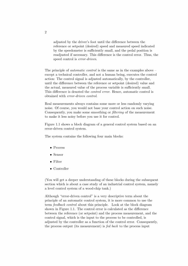
Figure 1.1 shows a block diagram of a general control system based on anerror-driven control system.

The system contains the following four main blocks:

• Process

• Sensor

• Filter

• Controller

(You will get a deeper understanding of these blocks during the subsequentsection which is about a case study of an industrial control system, namelya level control system of a wood-chip tank.)

Although “error-driven control” is a very descriptive term about theprinciple of an automatic control system, it is more common to use theterm feedback control about this principle. Look at the block diagramshown in Figure 1.1. The control error is calculated as the differencebetween the reference (or setpoint) and the process measurement, and thecontrol signal, which is the input to the process to be controlled, isadjusted by the controller as a function of the control error. Consequently,the process output (its measurement) is fed back to the process input

3

Process

Sensor

ySP ueController

y

dControlerror

Processmeasure-

ment

ym

n Measurement noise

Referenceor

Setpoint

Controlvariable

Process output variable

Feedback

Filterym,f

Filteredmeasure-

ment

Disturbance(environmental

variable)

Control loop

Figure 1.1: Block diagram of an error-driven control system

variable (control signal) via the controller. Hence, error-driven controlimplies feedback control.

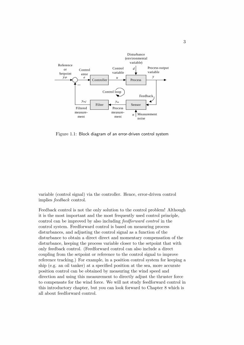
Feedback control is not the only solution to the control problem! Althoughit is the most important and the most frequently used control principle,control can be improved by also including feedforward control in thecontrol system. Feedforward control is based on measuring processdisturbances, and adjusting the control signal as a function of thedisturbance to obtain a direct direct and momentary compensation of thedisturbance, keeping the process variable closer to the setpoint that withonly feedback control. (Feedforward control can also include a directcoupling from the setpoint or reference to the control signal to improvereference tracking.) For example, in a position control system for keeping aship (e.g. an oil tanker) at a specified position at the sea, more accurateposition control can be obtained by measuring the wind speed anddirection and using this measurement to directly adjust the thruster forceto compensate for the wind force. We will not study feedforward control inthis introductory chapter, but you can look forward to Chapter 8 which isall about feedforward control.

4

1.2 A case study: Level control of wood-chiptank

1.2.1 Description of the control system with P&I diagramand block diagram

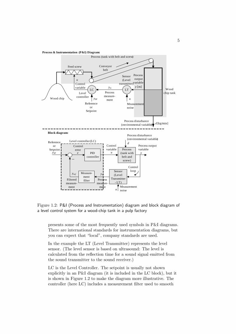
We will study an example of a real industrial control system. Figure 1.2shows a level control system for a wood-chip tank with feed screw andconveyor belt which runs with constant speed. Wood-chip is consumed viaan outlet screw in the bottom of the tank.1 2 3 The purpose of the controlsystem is to keep the measured chip level ym equal to a level setpoint ySP ,despite variations of the outflow, which is a process disturbance d.

The level control system works as follows (a more detailed description ofhow the control system works is given in Section 1.2.2): The controllertries to keep the measured level equal to the level setpoint by adjusting therotational speed — and thereby the chip flow — of the feed screw as afunction of the control error (which is the difference between the levelsetpoint and the measured level).

A few words about the need for a level control system for this chip tank:Hydrogene sulphate gas from the pulping process later in the productionline is used to preheat the wood chip. If the chip level in the tank is toolow, too much (stinking) gas is emitted to the athmosphere, causingpollution. With level control the level is kept close to a desired value(set-point) at which only a small amount of gas is expired. The level mustnot be too high, either, to avoid overflow and reduced preheating.

In Figure 1.2 the control system is documented in two ways:

• Process and instrumentation diagram or P&I diagram whichis a common way to document control systems in the industry. Thisdiagram contains easily recognizable drawings and symbols of theprocess to be controlled, together with symbols for the controllersand the sensors and the signals in the control system. Appendix A

1This example is based on an existing system in the paper pulp factory Södra Cell Toftein Norway. The tank with conveyor belt is in the beginning of the paper pulp productionline.

2The tank height is 15 m. The diameter is 4.13 m, and the cross-sectional area is13.4 m2. The nominal wood-chip outflow (and inflow at steady state) is 1500 kg/min.The conveyor belt is 200 m long, and runs with fixed speed. The transportation time(time-delay) of the belt is 250 sec = 4.17 min.

3A simulator of the system is available at http://techteach.no/simview.

5

y [m]

Wood chip

Wood chip tank

u

d [kg/min]

LTLC

Feed screw

Process(tank with belt and screw)

Sensor(Level

Transmitter- LT)

ySP ue PID controller

y

d

Block diagram:

Process & Instrumentation (P&I) Diagram:

Level controller

Sensor (Level

transmitter)Controlvariable

Processoutput

variable

Process disturbance(environmental variable)

Controlerror

Process measure-

ment

ym

Processmeasure-

ment

ym

nMeasurement noise

Referenceor

SetpointControlvariable


Level controller (LC)

Controlloop

Measure-mentfilter

ym,f

Filteredmeasure-

ment

Conveyor belt

Referenceor

Setpoint

ySP

Measurement noise

n

Process (tank with belt and screw)

Process disturbance(environmental variable)

Figure 1.2: P&I (Process and Instrumentation) diagram and block diagram ofa level control system for a wood-chip tank in a pulp factory

presents some of the most frequently used symbols in P&I diagrams.There are international standards for instrumentation diagrams, butyou can expect that “local”, company standards are used.

In the example the LT (Level Transmitter) represents the levelsensor. (The level sensor is based on ultrasound: The level iscalculated from the reflection time for a sound signal emitted fromthe sound transmitter to the sound receiver.)

LC is the Level Controller. The setpoint is usually not shownexplicitly in an P&I diagram (it is included in the LC block), but itis shown in Figure 1.2 to make the diagram more illustrative. Thecontroller (here LC) includes a measurement filter used to smooth

6

noisy measurement. It is not common to show the filter explicitely inP&I diagrams.

• Block diagram which is useful in principal and conceptualdescription of a control system.

Below are comments about the systems and variables (signals) in the blockdiagram shown in Figure 1.2.

Systems in Figure 1.2:

• The process is the physical system which is to be controlled.Included in the process is the actuator, which is the equipment withwhich (the rest of) the process is controlled.

In the example the process consists of the tank with the feed screwand the conveyor belt.

• The controller is typically in the form of a computer programimplemented in the control equipment. The controller adjusts thecontrol signal used to control or manipulate the process. Thecontroller calculates the control signal according some mathematicalformula defining the controller function. The controller functiondefines how to adjust the control signal as a function of the controlerror (which is the difference between the setpoint and the processmeasurement).

• The sensor measures the process variable to be controlled. Thephysical signal from the sensor is an electrical signal, voltage orcurrent. In industry 4—20 mA is the most common signal range ofsensor signals. (In the example the sensor is an ultrasound levelsensor, as mentioned earlier.)

• The measurement filter is a function block which is available inmost computer-based automation systems. The filter attenuates orsmooths out the inevitable random noise which exists in themeasurement signal. The measurement filter is described in detail inSection 7.2.2.

• The control loop or feedback loop is the closed loop consistingof the process, the sensor, the measurement filter, and the controllerconnected in a series connection.

Variables (signals) in Figure 1.2:

7

• The control variable or the manipulating variable is thevariable which the controller uses to control or manipulate theprocess. In this book u is used as a general symbol of the controlvariable. In commercial equipment you may see the symbol MV(manipulating variable).

In the example the control variable (or control signal) adjust the flowthrough the feed screw.

• The process output variable is the variable to be controlled sothat it becomes equal to or sufficiently close to the setpoint. In thisbook y is used as a general symbol of the process output variable. Incommercial control equipment PV (process variable or process value)may be used as a symbol.

In the example the wood chip level in the tank is the process outputvariable.

Note: The process output variable is not necessarily a physicaloutput from the process! In our example the chip outflow is not theprocess output variable. The chip outflow is actually a processdisturbance, see below.

• The disturbance is a non—controlled input variable to the processwhich affects the process output variable. From the control system’sperspective, this influence on the process output variable isundesirable, and the controller will adjust the control variable tocompensate for the influence. In this book, d is used as a generalsymbol for the disturbance. Typically, there are more than onedisturbances acting on a process.

In the example the chip outflow from the bottom of the tank is the(main) disturbance as it tends to bring the process variable (level)away from the level setpoint. Other disturbances are variations inthe inlet flow due to e.g. chip density variations.

• The setpoint or the reference is the desired or specified value ofthe process output variable. The general symbol ySP will be used inthis book.

In the example the desired level is the setpoint. A typical value forthis tank is 10 meters.

• The measurement signal is the output signal from the sensorwhich measures the process variable.

In the example the measurement signal is a current signal in therange 4 — 20 mA corresponding to level 0 — 15 m.

8

• The measurement noise is typically a random component in themeasurement signal. In practice all sensors produce noisemeasurements. The noise is propagated via the controller to thecontrol signal, which therefore can have abrupt variations, which maybe a serious problem for a control system. The measurement noisemay have various sources:

— It can be electronic (induced) noise.

— It can be noise due to the measurement principle, as when aultrasound sensor is used to measure the level of a wavy liquidsurface.

— It can be noise due to the limited resolution of theanalog-to-digital (AD) converter which converts the voltage orcurrent measurement signal into a number to be used in theautomation computer.

In the example the measurement noise stems from the AD converterand from the irregular surface of the chip surface in the tank.

• The control error is the difference between the setpoint and theprocess output variable:

e = ySP − y (1.1)

Since the process output variable is known via its measurement, thecontrol error is actually calculated as the difference between thesetpoint and the measurement, and it is expressed in a proper unit,e.g. meter or percent.

1.2.2 How the level control system works

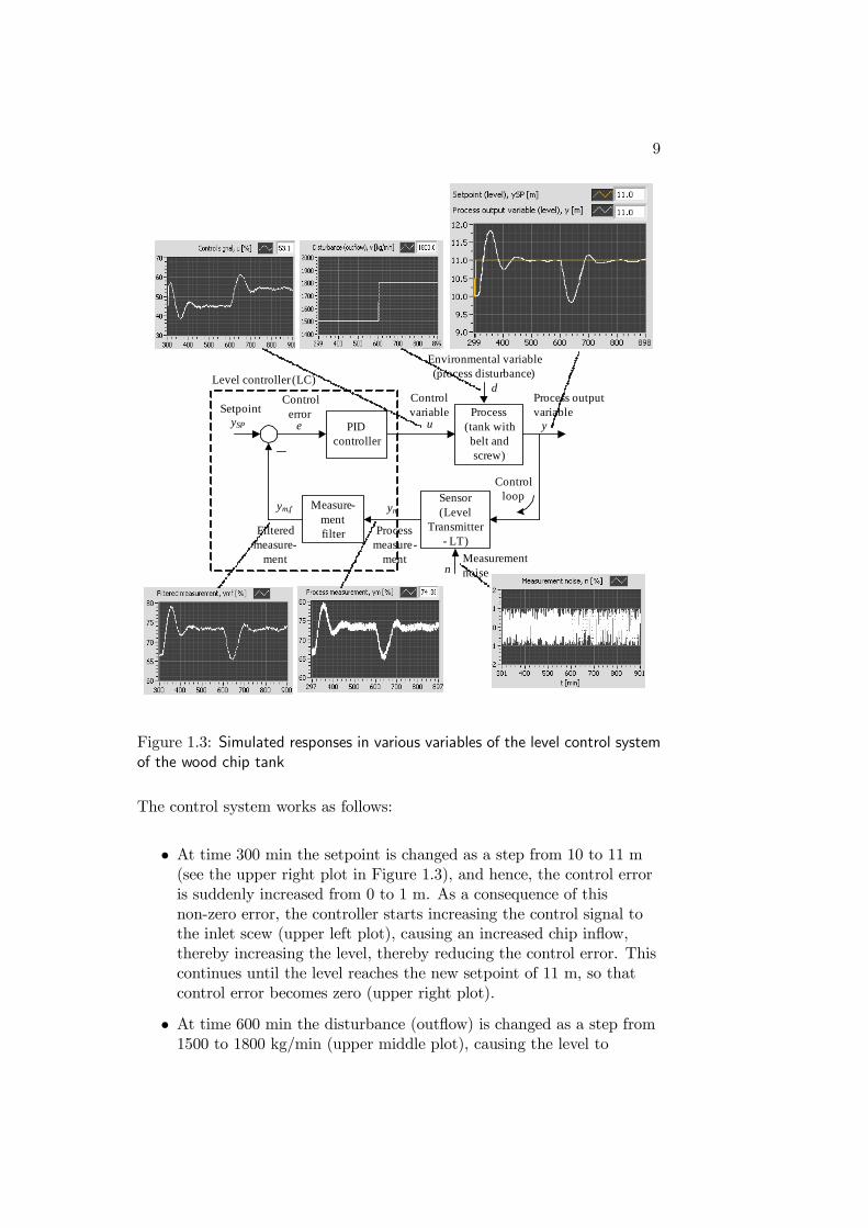
Figure 1.3 shows simulated responses in various variables of the system.4

Initially, the control signal is u = 45 % (it can be shown that this controlsignal is producing a chip inflow of 1500 kg/min which equals the initialoutflow), and the level is at the setpoint value of 10 m, so the initialcontrol error is zero. Random measurement noise is added to the levelmeasurement.

The controller is a PI controller (proportional plus integral) which is themost commonly used controller function in industry. The PI controller,which is a special case of the more general PID controller (proportionalplus integral plus derivative), is described in detail in Section 7.3.

4Parameter values of the system can be found on the front panel of the simulator ofthe system which is available at http://techteach.no/simview.

9

Process (tank with belt and screw)

Sensor(Level

Transmitter - LT)

ySP ue PID controller

y

dControlerror

Processmeasure-

ment

ym

nMeasurement noise

SetpointControlvariable


Level controller (LC)

Controlloop

Measure-mentfilter

ym,f

Filteredmeasure-

ment

Environmental variable(process disturbance)

Figure 1.3: Simulated responses in various variables of the level control systemof the wood chip tank

The control system works as follows:

• At time 300 min the setpoint is changed as a step from 10 to 11 m(see the upper right plot in Figure 1.3), and hence, the control erroris suddenly increased from 0 to 1 m. As a consequence of thisnon-zero error, the controller starts increasing the control signal tothe inlet scew (upper left plot), causing an increased chip inflow,thereby increasing the level, thereby reducing the control error. Thiscontinues until the level reaches the new setpoint of 11 m, so thatcontrol error becomes zero (upper right plot).

• At time 600 min the disturbance (outflow) is changed as a step from1500 to 1800 kg/min (upper middle plot), causing the level to

10

decrease, and hence the control error becomes different from zero.The operation of the control system is as after the setpoint change:Because of the non-zero error, the controller starts increasing thecontrol signal to the inlet scew, causing an increased chip inflow,thereby increasing the level, thereby reducing the control error. Thiscontinues until the level is at the setpoint of 11 m again.

• The measurement noise is smoothed by the measurement filter, butthe noise is not completely removed (lower plots).

• The remaining measurement noise (what remains despite thefiltering) is propagated through the controller, causing the controlsignal to be somewhat noisy (upper left plot).

1.3 The importance of control

In the previous sections we studied a level control system of a wood-chiptank. In general, the following process variables are controlled in industrialand other kinds of technical applications:

• Level or mass (of e.g. a storage tank)

• Pressure (in a chemical reactor)

• Temperature (in a room; in the fluid passing a heat exchanger; in areactor; in a greenhouse)

• Flow (of feeds into a reactor)

• pH (of a reactor)

• Chemical composition (of nitric acid; fertilizers, polypropylene)

• Speed (of a motor; a car)

• Position (of a ship; a painting robot arm; the tool of a cuttingmachine; a rocket)

Application of control may be of crucial importance to obtain the followingaims:

11

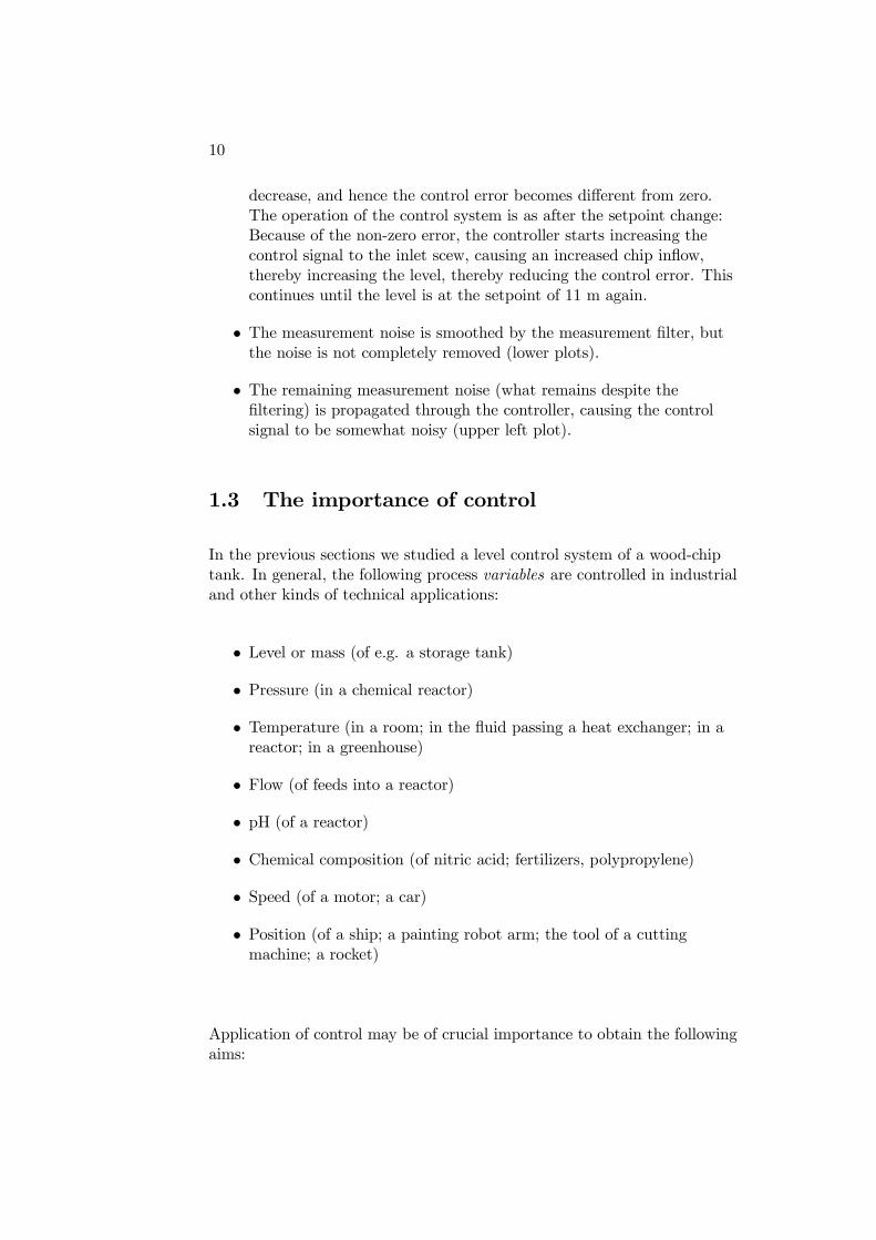
• Good product quality: A product will have acceptable qualityonly if the difference between certain process variables and theirsetpoint values — this difference is called the control error — are keptless than specified values. Proper use of control engineering may benecessary to achieve a sufficiently small control error, see Figure 1.4.

t t

Maxlimit

Minlimit

Without control or withpoor control

With good control

Setpoint, ySP

Process output, y

Less error!(Smaller variance)

Control error,e = ySP - y

Figure 1.4: Good control reduces the control error

One example: In fertilizers the pH value and the composition ofNitrogen, Phosphate and Potassium are factors which express thequality of the fertilizer (for example, too low pH value is not good forthe soil). Therefore the pH value and the compositions must becontrolled.

• Good production economy: The production economy will becomeworse if part of the products has unacceptable quality so that it cannot be sold. Good control may maintain the good product quality,and hence, contribute to good production economy. Further, by goodcontrol it may be possible to tighten the limits of the quality so thata higher price may be taken for the product!

• Safety: To guarantee the security both for humans and equipment,it may be required to keep variables like pressure, temperature, level,and others within certain limits— that is, these variables must becontrolled. Some examples:

— An aircraft with an autopilot (an autopilot is a positionalcontrol system).

— A chemical reactor where pressure and temperature must becontrolled.

12

• Environmental care: The amount of poisons to be emitted from afactory is regulated through laws and directions. The application ofcontrol engineering may help to keep the limits. Some examples:

— In a wood chip tank in a paper pulp factory, hydrogene sulfategas from the pulp process is used to preheat the wood chip. Ifthe chip level in the tank is too low, too much (stinking) gas isemitted to the atmosphere, causing pollution. With levelcontrol the level is kept close to a desired value (set-point) atwhich only a small amount of gas is expired.

— In the so-called washing tower nitric acid is added to theintermediate product to neutralize exhaust gases from theproduction. This is accomplished by controlling the pH value ofthe product by means of a pH control system. Hence, the pHcontrol system ensures that the amount of emitted ammonia isbetween specified limits.

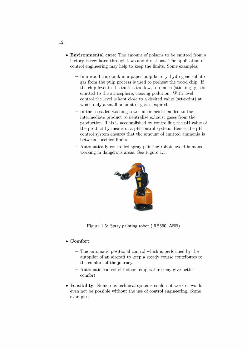
— Automatically controlled spray painting robots avoid humansworking in dangerous areas. See Figure 1.5.

Figure 1.5: Spray painting robot (IRB580, ABB)

• Comfort:

— The automatic positional control which is performed by theautopilot of an aircraft to keep a steady course contributes tothe comfort of the journey.

— Automatic control of indoor temperature may give bettercomfort.

• Feasibility: Numerous technical systems could not work or wouldeven not be possible without the use of control engineering. Someexamples:

13

— An exothermal reactor operating in an unstable (but optimal)operating point

— Launching a space vessel (the course is stabilized)

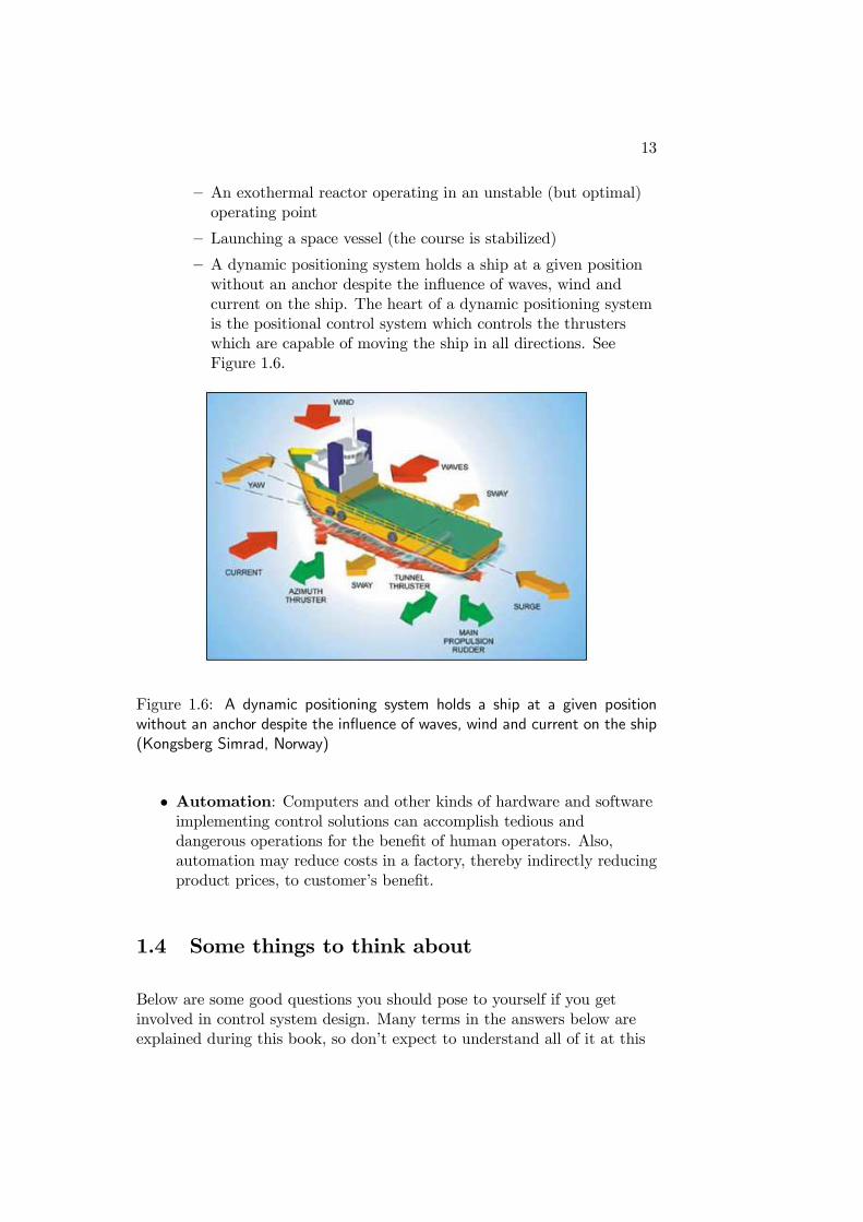
— A dynamic positioning system holds a ship at a given positionwithout an anchor despite the influence of waves, wind andcurrent on the ship. The heart of a dynamic positioning systemis the positional control system which controls the thrusterswhich are capable of moving the ship in all directions. SeeFigure 1.6.

Figure 1.6: A dynamic positioning system holds a ship at a given positionwithout an anchor despite the influence of waves, wind and current on the ship(Kongsberg Simrad, Norway)

• Automation: Computers and other kinds of hardware and softwareimplementing control solutions can accomplish tedious anddangerous operations for the benefit of human operators. Also,automation may reduce costs in a factory, thereby indirectly reducingproduct prices, to customer’s benefit.

1.4 Some things to think about

Below are some good questions you should pose to yourself if you getinvolved in control system design. Many terms in the answers below areexplained during this book, so don’t expect to understand all of it at this

14

moment. You may read this section again after you have completed thebook!

• Is there really a need for control? Yes, there is a need forcontrol if there is a chance that the process output variable will drifttoo far away from its desired value. Such a drift can be caused bysevere variations of environmental variables (process disturbances).For unstable processes, like water tanks and exothermal reactors andmotion systems like robots and ships which must be positioned, therewill always be a need for control to keep the process output variable(level; temperature; position, respectively) at a setpoint or referencevalue.

• Which process variable(s) needs to be controlled? (To makeit become equal to a setpoint or reference value.) Liquid level in agiven tank? Pressure of vapour in the tank? Temperature? Flow?Composition?

• How to measure that process variable? Select an appropriatesensor, and make sure it detects the value of the process variablewith as little time-delay and sluggishness as possible! In other words,measure as directly as you can.

• Is the measurement signal noisy? It probably is. Use a lowpassfilter to filter or smooth out the noise, but don’t make the filteringtoo strong — or you will also filter out significant contents of themeasurement signal, causing the controller to react on erroneousinformation.

• How to manipulate the process variable? Select an actuatorthat gives a strong impact on the process variable (to be controlled)!Avoid time-delays if possible, because time-delays in a control loopwill limit the speed of the control, and you may get a sluggish controlloop, causing the control error to become large after disturbancevariations.

• Which controller function (in the feedback controller)? Trythe standard PID controller. Note that most PID controllers actuallyoperate as PI controllers since the derivative (D) term is deactivatedbecause it amplifies measurement noise through the controller,causing noisy control signal which may cause excessive wear of amechanical actuator.

• How to tune the controller?

15

If you don’t have mathematical model of the process to be controlled,try the Good Gain method, which is a simple, experimental tuningmethod.

If you do have a mathematical process model, try Skogestad’smodel-based tuning method to get the controller parameters directlyfrom the process model parameters. Alternatively, with a model, youcan create a simulator of your control system in e.g. LabVIEW orSimulink or Scicos, and then apply the Good Gain method on thesimulator.

If your controller has an Auto-tune button, try it!

• Is the stability of the control system good? The mostimportant requirement to a control system is that it has goodstability. In other words, the responses should show good damping(well damped oscillations). The responses in the level control systemwhich are shown in Figure 1.3 indicate good stability!

If you don’t have a mathematical model of the system, apply a (small)step change of the setpoint and observe whether the stability of thecontrol system is ok. If you think that the stability is not goodenough (too little damping of oscillations), try reducing thecontroller gain and increasing the integral time somewhat, say by afactor of two. Also, derivative control action can improve stability ofthe control loop, but remember the drawback of the D-term relatedto amplification of random measurement noise.

If you do have a mathematical model of the control system, create asimulator, and simulate responses in the process variable and thecontrol variable due to step changes in the setpoint and thedisturbances (load variables), e.g. environmental temperature, feedcomposition, external forces, etc. With a simulator, you may alsowant to make realistic changes of certain parameters of the processmodel, for example time-delays or some other physical parameters, tosee if the control system behaves well despite these parameterchanges (assuming the controller is not tuned again). In this way youcan test the robustness of the control system against processvariations. If the control system does not behave well, for examplehaving too poor stability, after the parameter changes, consider Gainscheduling which is based on changing the PID parametersautomatically as functions of certain process parameters.

• Is the control error small enough after disturbance changes,and after setpoint changes?

If you do not have a simulator of the control system, it may bedifficult to generate disturbance changes yourself, but setpoint

16

changes can of course be applied easily.

If you have a simulator, you can apply both setpoint changes anddisturbance changes.

If — using either experiments or simulator — the control error is toolarge after the changes of the setpoint and the disturbance, try totune the controller again to obtain faster control.

• Still not happy with control system performance afterretuning the controller? Then, look for other control structuresor methods based on exploiting more process information:

— Feedforward control : This requires that you measure one ormore of the disturbances (load variables) acting on the process,and using these measurements to directly adjust the controlsignal to compensate for the disturbance(s).

— Cascade control : This requires that you measure some internalprocess variable which is influenced by the disturbance, andconstruct an inner control loop (inside the main control loop)based on this internal measurement to quickly compensate forthe disturbance.

— Model-based control : Consider for example optimal control withstate-variable feedback (LQ (Linear Quadratic) optimalcontrol), or model-based predicitive control (MPC). [2]

1.5 About the contents and organization of thisbook

This book contains two main parts:

• Part One: Process models and dynamics which presents thebasic theory of mathematical process models and dynamics. Thissystems theory is useful for practical process control mainly becauseit makes it possible to implement simulators of control systems.With simulators you can test a virtual or a real (practical) controlsystem. The purpose of such tests can be design, analysis, oroperator (and student) training. Industry uses simulator-baseddesign and training more and more. The systems theory is useful alsobecause it gives you tools to represent and to characterize variouscomponents of a control system.

17

• Part Two: Feedback and feedforward control which presentspractical control methods with emphasis on feedback control withPID (proportional + integral + derivative) controllers which arecommonly used in the industry. Feedforward control is alsodescribed. Furthermore, several control structures based on the PIDcontroller are described, as cascade control, ratio control, andplantwide control principles. Also, sequential control usingSequential function charts is described.

Part I

PROCESS MODELS ANDDYNAMICS

19

Chapter 2

Representation of differentialequations with blockdiagrams and state-spacemodels

2.1 Introduction

The basic mathematical model form for dynamic systems is the differentialequation. This is because the basic modeling principle — denoted theBalance Law or Conservation principle — used to develop a model results inone of more differential equations describing the system. These modelingprinciples are described in Chapter 3. The present chapter shows you howto represent a given differential equation as block diagrams and state-spacemodels:

• Block diagrams give good information of the structure of the model,e.g. how subsystems are connected. And what is more important:With block diagrams you can build simulators in graphicalsimulation tools as SIMULINK and LabVIEW Simulation Module.

• State-space models are a standardized form of writing the differentialequations. All the time-derivatives in the model are of first order,and they appear on the left-hand side of the differential equations.Various tools for analysis and design and simulation of dynamicsystems and control systems assume state models. However, thisbook does not cover state-space analysis and design (a reference is

21

22

[2]), and concerning simulation it is my view that it is more useful touse block diagrams than state-space models as the basis for creatingsimulation models. Still, the concept of state-space models isintroduced here because you may meet it in certain contexts (e.g.literature) related to basic dynamics and control.

2.2 What is a dynamic system?

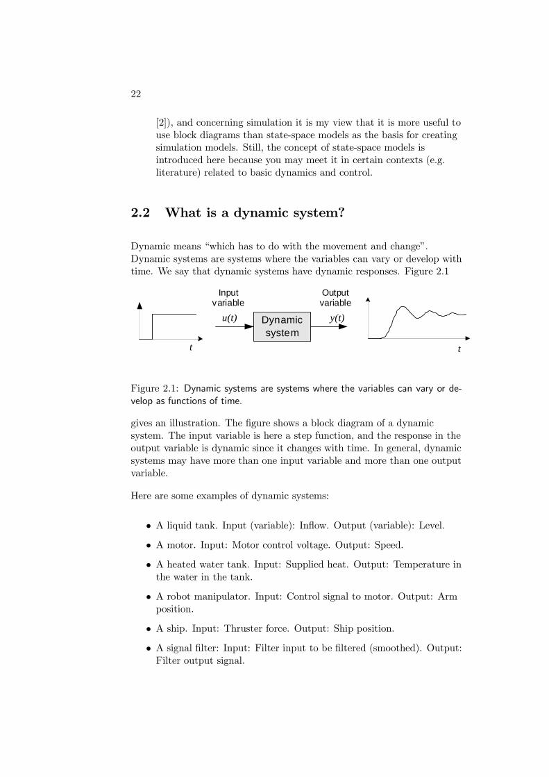
Dynamic means “which has to do with the movement and change”.Dynamic systems are systems where the variables can vary or develop withtime. We say that dynamic systems have dynamic responses. Figure 2.1

Dynamicsystem

u(t)

t

y(t)

t

Inputvariable

Outputvariable

Figure 2.1: Dynamic systems are systems where the variables can vary or de-velop as functions of time.

gives an illustration. The figure shows a block diagram of a dynamicsystem. The input variable is here a step function, and the response in theoutput variable is dynamic since it changes with time. In general, dynamicsystems may have more than one input variable and more than one outputvariable.

Here are some examples of dynamic systems:

• A liquid tank. Input (variable): Inflow. Output (variable): Level.

• A motor. Input: Motor control voltage. Output: Speed.

• A heated water tank. Input: Supplied heat. Output: Temperature inthe water in the tank.

• A robot manipulator. Input: Control signal to motor. Output: Armposition.

• A ship. Input: Thruster force. Output: Ship position.

• A signal filter: Input: Filter input to be filtered (smoothed). Output:Filter output signal.

23

• A control system for a physical process: Input: Setpoint. Output:Process output variable.

2.3 Mathematical block diagrams

2.3.1 Commonly used blocks in block diagrams

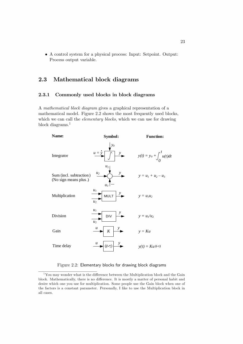
A mathematical block diagram gives a graphical representation of amathematical model. Figure 2.2 shows the most frequently used blocks,which we can call the elementary blocks, which we can use for drawingblock diagrams.1

Ku y

Gain

u2 ySum (incl. subtraction)

u3

u = y yIntegrator

y0

u yTime delay

u1

MULTy

Multiplicationu1

u2

DIVy

Division

u1

u2

y = u1 + u2 – u3

y = u1u2

y = u1/u2

y = Ku

y(t) = Ku

y(t) = y0 + u(t)dtt

0

Symbol: Function:Name:

(No sign means plus .)

Figure 2.2: Elementary blocks for drawing block diagrams

1You may wonder what is the difference between the Multiplication block and the Gainblock. Mathematically, there is no difference. It is mostly a matter of personal habit anddesire which one you use for multiplication. Some people use the Gain block when one ofthe factors is a constant parameter. Personally, I like to use the Multiplication block inall cases.

24

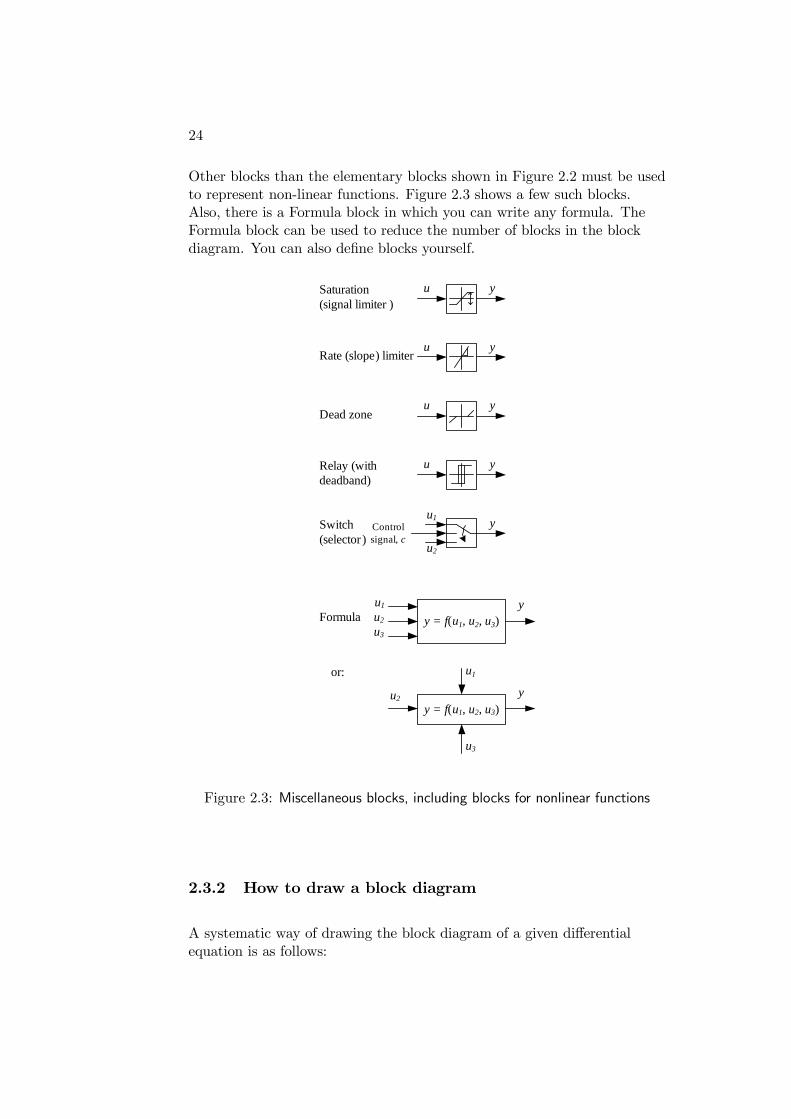
Other blocks than the elementary blocks shown in Figure 2.2 must be usedto represent non-linear functions. Figure 2.3 shows a few such blocks.Also, there is a Formula block in which you can write any formula. TheFormula block can be used to reduce the number of blocks in the blockdiagram. You can also define blocks yourself.

u yRate (slope) limiter

Dead zone

u ySaturation(signal limiter )

Relay (with deadband)

Switch(selector)

u y

Controlsignal, c

y

u y

u1

u2

y = f(u1, u2, u3)yu1

u2

u3

Formula

y = f(u1, u2, u3)y

u1

u3

or:

u2

Figure 2.3: Miscellaneous blocks, including blocks for nonlinear functions

2.3.2 How to draw a block diagram

A systematic way of drawing the block diagram of a given differentialequation is as follows:

25

1. Write the differential equations so that the variable of the highesttime-derivative order appears alone on the left part of the equations.

2. For first order differential equations (first order time-derivatives):Draw one integrator for each of the variables that appear with itstime-derivative in the model, so that the time-derivative is at theintegrator input and the variable itself is at the integrator output.

For second order differential equations (second ordertime-derivatives): Draw two integrators (from left to right) andconnect them in series. The second order time-derivative is then theinput to the leftmost integrator.

You will probably not see third or higher order differential equations,but if you do, the above procedure is naturally extended.

The variables at the integrator outputs can be regarded as thestate-variables of the system because their values at any instant oftime represent the state of the system. The general names of thestate-variables are x1, x2 etc. The initial values of the state-variablesare the initial outputs of the integrator. (More about state-spacemodels in Section 2.4.)

3. Connect the integrators together according to the differentialequation using proper blocks, cf. Figures 2.2 and 2.3. Alternatively,to use less blocks, you can include one

The following example demonstrates the above procedure.

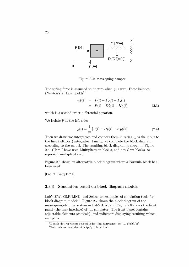
Example 2.1 Block diagram of mass-spring-damper system

Figure 2.4 shows a mass-spring-damper-system.2 y is position. F isapplied force. D is damping constant. K is spring constant. It is assumedthat the damping force Fd is proportional to the velocity:

Fd(t) = Dy(t) (2.1)

and that the spring force Fs is proportional to the position of the mass:

Fs(t) = Ky(t) (2.2)

2The mass-spring-damper system is not a typical system found in process control. It ischosen here because it is easy to develop a mathematical model using well known physicalprinciples, here the Newton’s second law. Examples of more relevance to process controlare described in Chapter 3.

26

m

K [N/m]

D [N/(m/s)]

F [N]

0 y [m]

Figure 2.4: Mass-spring-damper

The spring force is assumed to be zero when y is zero. Force balance(Newton’s 2. Law) yields3

my(t) = F (t)− Fd(t)− Fs(t)

= F (t)−Dy(t)−Ky(t) (2.3)

which is a second order differential equation.

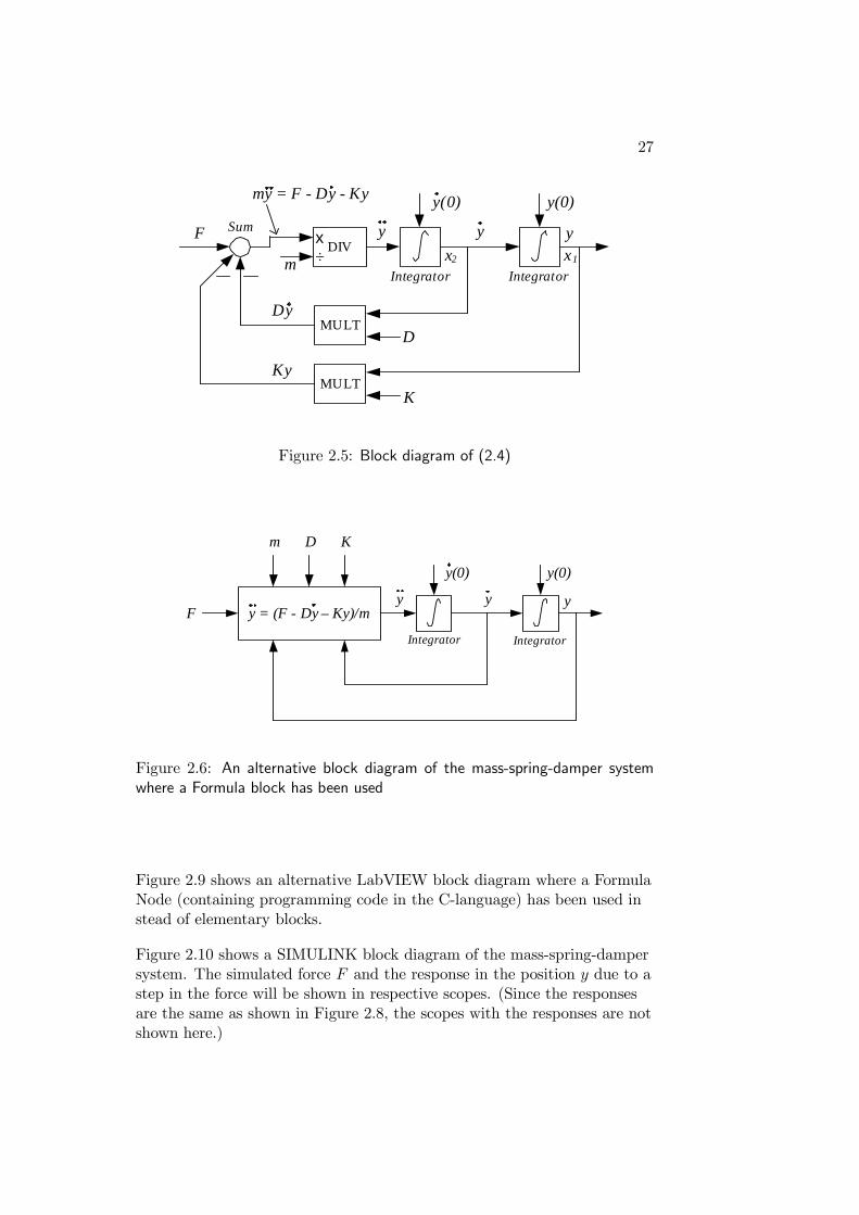
We isolate y at the left side:

y(t) =1

m[F (t)−Dy(t)−Ky(t)] (2.4)

Then we draw two integrators and connect them in series. y is the input tothe first (leftmost) integrator. Finally, we complete the block diagramaccording to the model. The resulting block diagram is shown in Figure2.5. (Here I have used Multiplication blocks, and not Gain blocks, torepresent multiplication.)

Figure 2.6 shows an alternative block diagram where a Formula block hasbeen used.

[End of Example 2.1]

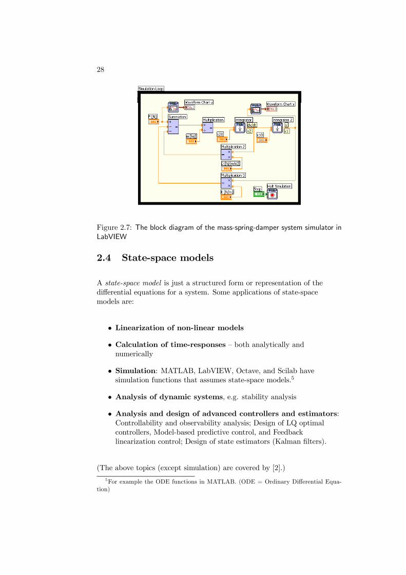
2.3.3 Simulators based on block diagram models

LabVIEW, SIMULINK, and Scicos are examples of simulation tools forblock diagram models.4 Figure 2.7 shows the block diagram of themass-spring-damper system in LabVIEW, and Figure 2.8 shows the frontpanel (the user interface) of the simulator. The front panel containsadjustable elements (controls), and indicators displaying resulting valuesand plots.

3Double-dot represents second order time-derivative: y(t) ≡ d2y(t)/dt24Tutorials are available at http://techteach.no.

27

Fx2

y(0)y(0)

x1DIV

m

Sum

Integrator Integrator

MULTD

MULTK

x÷

Dy

Ky

y yy

my = F - Dy - Ky

Figure 2.5: Block diagram of (2.4)

F

y(0)y(0)

m

Integrator Integrator

D K

y yyy = (F - Dy – Ky)/m

Figure 2.6: An alternative block diagram of the mass-spring-damper systemwhere a Formula block has been used

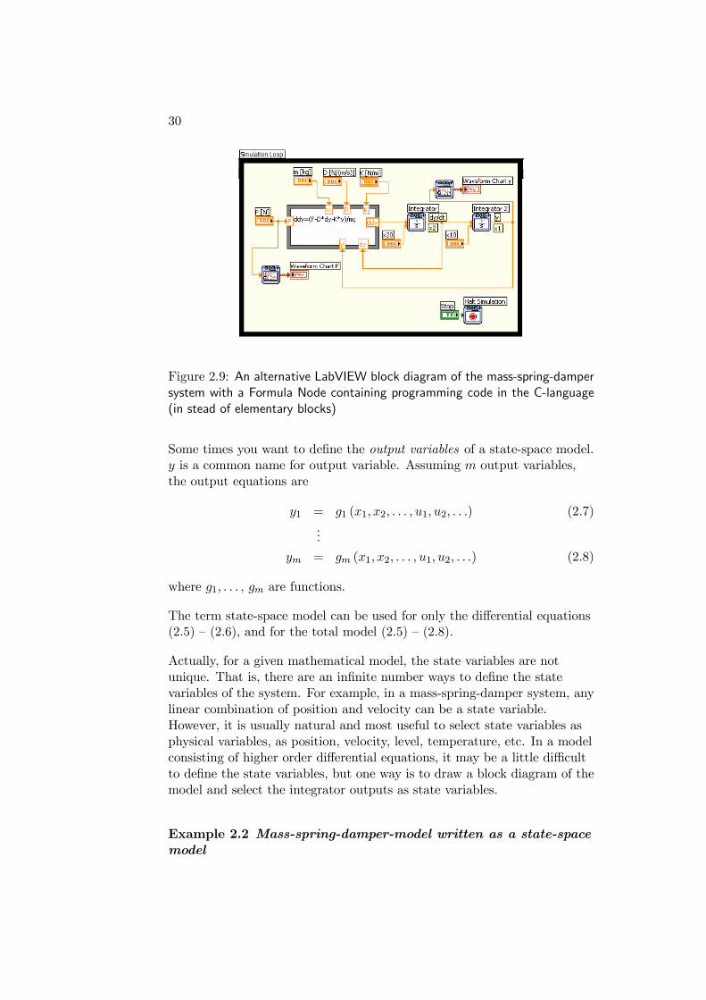
Figure 2.9 shows an alternative LabVIEW block diagram where a FormulaNode (containing programming code in the C-language) has been used instead of elementary blocks.

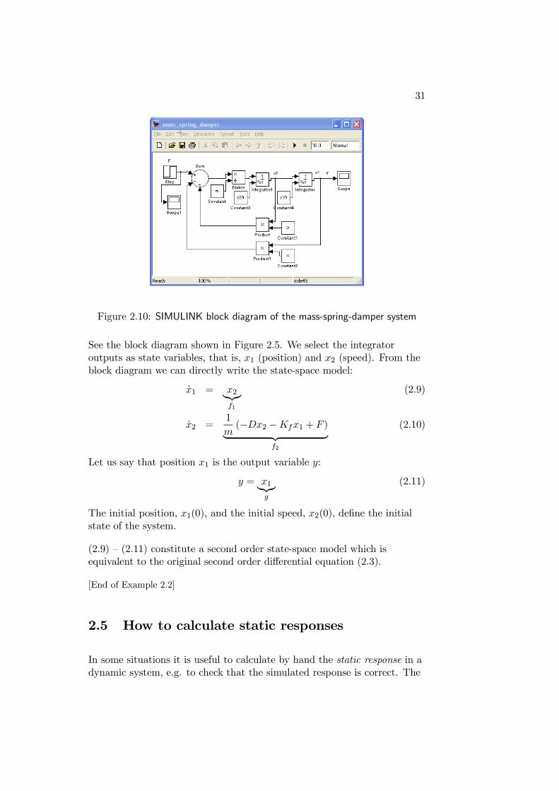
Figure 2.10 shows a SIMULINK block diagram of the mass-spring-dampersystem. The simulated force F and the response in the position y due to astep in the force will be shown in respective scopes. (Since the responsesare the same as shown in Figure 2.8, the scopes with the responses are notshown here.)

28

Figure 2.7: The block diagram of the mass-spring-damper system simulator inLabVIEW

2.4 State-space models

A state-space model is just a structured form or representation of thedifferential equations for a system. Some applications of state-spacemodels are:

• Linearization of non-linear models

• Calculation of time-responses — both analytically andnumerically

• Simulation: MATLAB, LabVIEW, Octave, and Scilab havesimulation functions that assumes state-space models.5

• Analysis of dynamic systems, e.g. stability analysis

• Analysis and design of advanced controllers and estimators:Controllability and observability analysis; Design of LQ optimalcontrollers, Model-based predictive control, and Feedbacklinearization control; Design of state estimators (Kalman filters).

(The above topics (except simulation) are covered by [2].)

5For example the ODE functions in MATLAB. (ODE = Ordinary Differential Equa-tion)

29

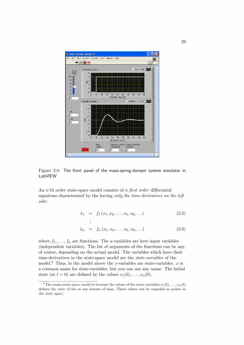
Figure 2.8: The front panel of the mass-spring-damper system simulator inLabVIEW

An n’th order state-space model consists of n first order differentialequations characterized by the having only the time-derivatives on the leftside:

x1 = f1 (x1, x2, . . . , u1, u2, . . .) (2.5)...

xn = fn (x1, x2, . . . , u1, u2, . . .) (2.6)

where f1, . . . , fn are functions. The u-variables are here input variables(independent variables). The list of arguments of the functions can be any,of course, depending on the actual model. The variables which have theirtime-derivatives in the state-space model are the state-variables of themodel.6 Thus, in the model above the x-variables are state-variables. x isa common name for state-variables, but you can use any name. The initialstate (at t = 0) are defined by the values x1(0), . . . , xn(0).

6The name state-space model is because the values of the state-variables x1(t), . . . , xn(t)defines the state of the at any instant of time. These values can be regarded as points inthe state-space.

30

Figure 2.9: An alternative LabVIEW block diagram of the mass-spring-dampersystem with a Formula Node containing programming code in the C-language(in stead of elementary blocks)

Some times you want to define the output variables of a state-space model.y is a common name for output variable. Assuming m output variables,the output equations are

y1 = g1 (x1, x2, . . . , u1, u2, . . .) (2.7)...

ym = gm (x1, x2, . . . , u1, u2, . . .) (2.8)

where g1, . . . , gm are functions.

The term state-space model can be used for only the differential equations(2.5) — (2.6), and for the total model (2.5) — (2.8).

Actually, for a given mathematical model, the state variables are notunique. That is, there are an infinite number ways to define the statevariables of the system. For example, in a mass-spring-damper system, anylinear combination of position and velocity can be a state variable.However, it is usually natural and most useful to select state variables asphysical variables, as position, velocity, level, temperature, etc. In a modelconsisting of higher order differential equations, it may be a little difficultto define the state variables, but one way is to draw a block diagram of themodel and select the integrator outputs as state variables.

Example 2.2 Mass-spring-damper-model written as a state-spacemodel

31

Figure 2.10: SIMULINK block diagram of the mass-spring-damper system

See the block diagram shown in Figure 2.5. We select the integratoroutputs as state variables, that is, x1 (position) and x2 (speed). From theblock diagram we can directly write the state-space model:

x1 = x2f1

(2.9)

x2 =1

m(−Dx2 −Kfx1 + F )

f2

(2.10)

Let us say that position x1 is the output variable y:

y = x1g

(2.11)

The initial position, x1(0), and the initial speed, x2(0), define the initialstate of the system.

(2.9) — (2.11) constitute a second order state-space model which isequivalent to the original second order differential equation (2.3).


2.5 How to calculate static responses

In some situations it is useful to calculate by hand the static response in adynamic system, e.g. to check that the simulated response is correct. The

32

static response is the steady-state value of the output variable of the modelwhen the input variables have constant values. This response can becalculated directly from the model after the time-derivatives have been setequal to zero, since then the variables have constant values, theirtime-derivatives equal zero.

Example 2.3 Calculation of static response formass-spring-damper

The mass-spring-damper system described in Example 2.1 has thefollowing model:

my = −Dy −Ky + F (2.12)

Suppose the force F is constant of value Fs. The corresponding staticresponse in the position y can be found by setting the time-derivativesequal to zero and solving with respect to y. The result is

ys =FsK

(2.13)

Let us use (2.13) to check the simulated response shown in Figure 2.8: Onthe front panel we see that Fs = 4 N, and K = 2 N/m. Thus,

ys =FsK=

4 N2 N/m

= 2 m (2.14)

which is the same as the simulated static value of y, cf. Figure 2.8.


Chapter 3

Mathematical modeling

3.1 Introduction

This chapter describes basic principles of mathematical modeling. Amathematical model is the set of equations which describe the behavior ofthe system. The chapter focuses on how to develop dynamic models, andyou will see that the models are differential equations. (How to representsuch differential equations as block diagrams, ready for implementation inblock diagram based simulators, was explained in Section 2.)

Unfortunately we can never make a completely precise model of a physicalsystem. There are always phenomena which we will not be able to model.Thus, there will always be model errors or model uncertainties. But even ifa model describes just a part of the reality it can be very useful foranalysis and design — if it describes the dominating dynamic properties ofthe system.1

This chapter describes modeling based on physical principles. Models canalso be developed from experimental (historical) data. This way ofmathematical modeling is called system identification. It is not covered bythe present book (an introduction is given in [2]).

1This is expressed as follows in [5]: “All models are wrong, but some are useful.”

33

34

3.2 A procedure for mathematical modeling

Below is described a procedure for developing dynamic mathematicalmodels for physical systems:

1. Define systems boundaries. All physical systems works ininteraction with other systems. Therefore it is necessary to define theboundaries of the system before we can begin developing amathematical model for the system, but in most cases defining theboundaries is done quite naturally.

2. Make simplifying assumptions. One example is to assume thatthe temperature in a tank is the same everywhere in the tank, thatis, there are homogeneous conditions in the tank.

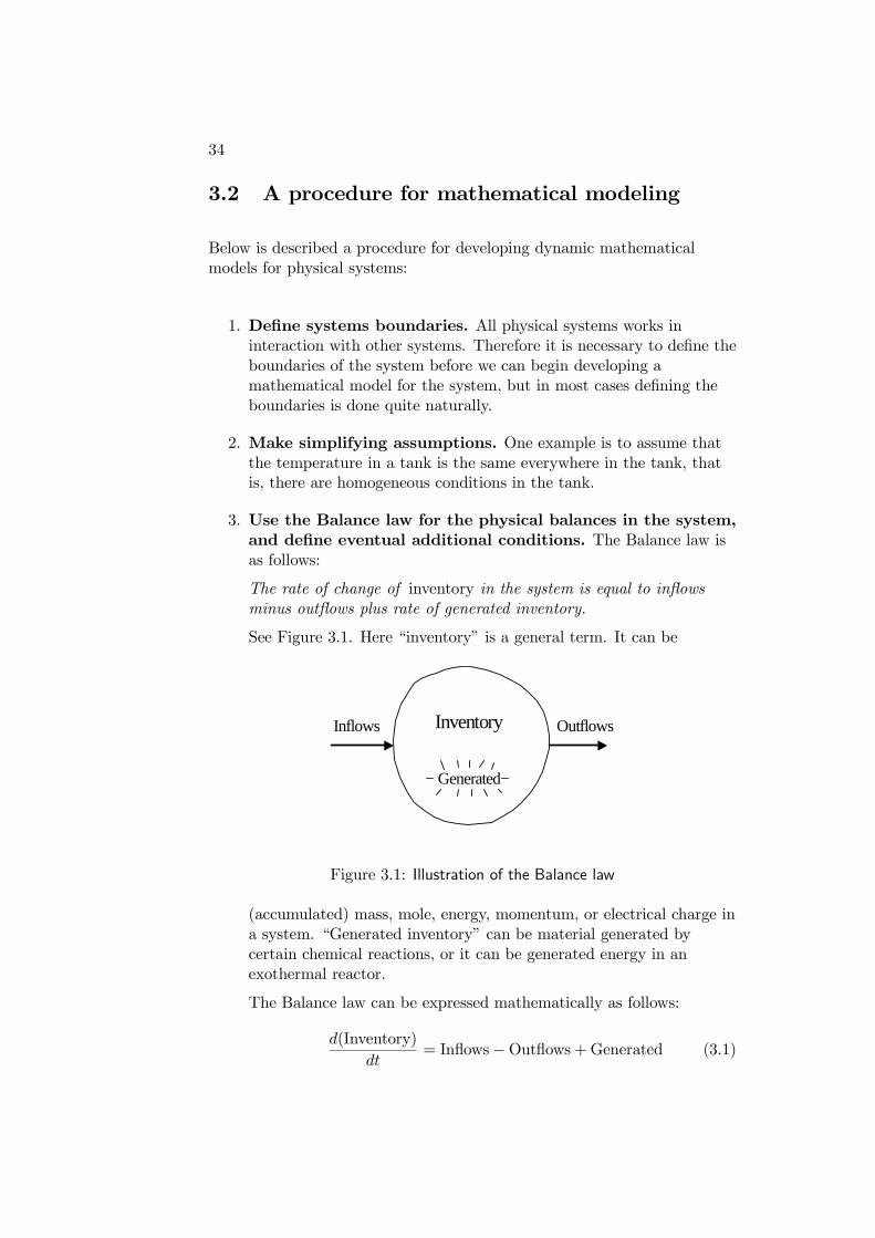
3. Use the Balance law for the physical balances in the system,and define eventual additional conditions. The Balance law isas follows:

The rate of change of inventory in the system is equal to inflowsminus outflows plus rate of generated inventory.

See Figure 3.1. Here “inventory” is a general term. It can be

InventoryInflows Outflows

Generated

Figure 3.1: Illustration of the Balance law

(accumulated) mass, mole, energy, momentum, or electrical charge ina system. “Generated inventory” can be material generated bycertain chemical reactions, or it can be generated energy in anexothermal reactor.

The Balance law can be expressed mathematically as follows:

d(Inventory)dt

= Inflows−Outflows+Generated (3.1)

35

The Balance law results in one ore more differential equations due tothe term d/dt. So, the model consists of differential equations.

You can define additional conditions to the model, like therequirement that the mass of liquid in a tank is not negative.

To actually calculate the amount of inventory in the system from themodel, you just integrate the differential equation (3.1), probablyusing a computer program (simulation tool). The inventory at time tis

Inventory(t) = Inventory(0)+ t

0(Inflows−Outflows+Generated) dθ

(3.2)where t = 0 is the initial time.

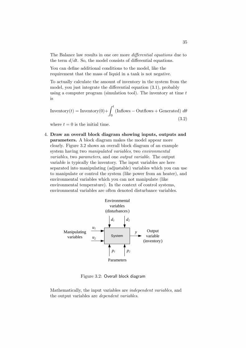
4. Draw an overall block diagram showing inputs, outputs andparameters. A block diagram makes the model appear moreclearly. Figure 3.2 shows an overall block diagram of an examplesystem having two manipulated variables, two environmentalvariables, two parameters, and one output variable. The outputvariable is typically the inventory. The input variables are hereseparated into manipulating (adjustable) variables which you can useto manipulate or control the system (like power from an heater), andenvironmental variables which you can not manipulate (likeenvironmental temperature). In the context of control systems,environmental variables are often denoted disturbance variables.

Systemy

Environmental variables

(disturbances)

u1

u2

Output variable

(inventory)

Manipulatingvariables

Parameters

d1 d2

p1 p2

Figure 3.2: Overall block diagram

Mathematically, the input variables are independent variables, andthe output variables are dependent variables.

36

The parameters of the model are quantities in the model whichtypically (but not necessarily) have constant values, like liquiddensity and spring constant. If a parameter have a varying value, itmay alternatively be regarded as an environmental variable — youdecide. To simplify the overall block diagram you can skip drawingthe parameters.

5. Present the model on a proper form. The most common modelforms are block diagrams (cf. Section 2.3), state models (cf. Section2.4), and transfer functions (cf. Section 5). The choice of model formdepends on the purpose of the model. For example, to tune a PIDcontroller using Skogestad’s method (Sec. 10.3) you need a transferfunction model of the process.

The following sections contains several examples of mathematical modeling.In the examples points 1 and 2 above are applied more or less implicitly.

3.3 Mathematical modeling of material systems

In a system where the mass may vary, mass is the “inventory” in theBalance law (3.1) which now becomes a mass balance:

dm(t)

dt=

i

Fi(t) (3.3)

where m [kg] is the mass, and Fi [kg/s] is mass inflow (no. i).

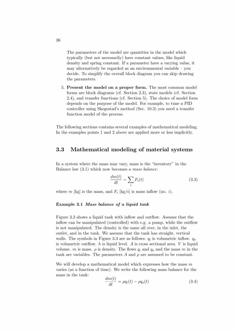
Example 3.1 Mass balance of a liquid tank

Figure 3.3 shows a liquid tank with inflow and outflow. Assume that theinflow can be manipulated (controlled) with e.g. a pump, while the outflowis not manipulated. The density is the same all over, in the inlet, theoutlet, and in the tank. We assume that the tank has straight, verticalwalls. The symbols in Figure 3.3 are as follows: qi is volumetric inflow. qois volumetric outflow. h is liquid level. A is cross sectional area. V is liquidvolume. m is mass. ρ is density. The flows qi and qo and the mass m in thetank are variables. The parameters A and ρ are assumed to be constant.

We will develop a mathematical model which expresses how the mass mvaries (as a function of time). We write the following mass balance for themass in the tank:

dm(t)

dt= ρqi(t)− ρqo(t) (3.4)

37

qi [m3/s]

A [m2]

[kg/m3]

qo [m3/s]

h [m]

0

m [kg]

V [m3]

Figure 3.3: Example 3.1: Liquid tank

which is a differential equation for m. An additional condition for thedifferential equation is m ≥ 0. (3.4) is a mathematical model for thesystem. ρ is a parameter in the model. Parameters are quantities whichusually have a constant values and which characterizes the model.

(3.4) is a differential equation for the mass m(t). Perhaps you are moreinterested in how level h will the vary? The correspondence between h andm is a given by

m(t) = ρV (t) = ρAh(t) (3.5)

We insert this into the mass balance (3.4), which then becomes

dm(t)

dt=

d [ρV (t)]

dt=

d [ρAh(t)]

dt= ρA

dh(t)

dt= ρqi(t)− ρqo(t) (3.6)

where ρ and A the parameters are moved outside the derivation (these areassumed to be constant). By cancelling ρ and dividing by A we get thefollowing differential equation for h(t):

dh(t)

dt= h(t) =

1

A[qi(t)− qo(t)] (3.7)

with the condition hmin ≤ h ≤ hmax.

Figure 3.4 shows an overall block diagram for the model (3.7). qi and qo areinput variables, which generally are variables which drive the system (weassume here that qo is independent of the level, as when it is manipulatedusing a pump). h is an output variable, which generally is the variablewhich expresses the response or a state of the system. Note that qo is an

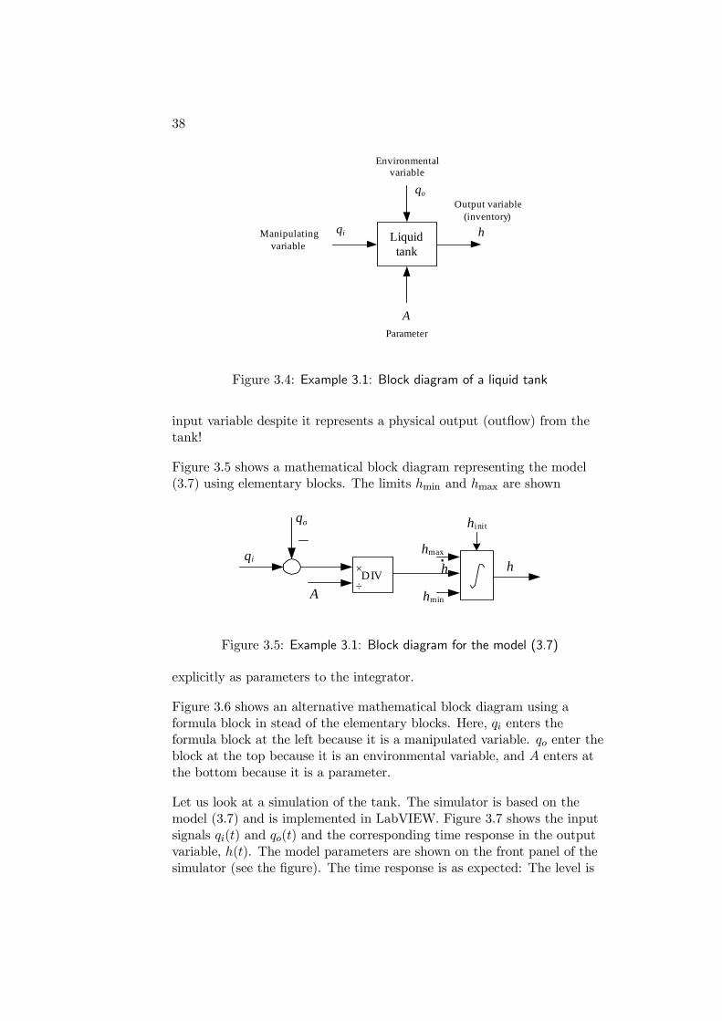
38

qo

Liquid tank

qi hManipulatingvariable

Output variable(inventory)

Environmentalvariable

AParameter

Figure 3.4: Example 3.1: Block diagram of a liquid tank

input variable despite it represents a physical output (outflow) from thetank!

Figure 3.5 shows a mathematical block diagram representing the model(3.7) using elementary blocks. The limits hmin and hmax are shown

hDIV h

.

A

×

÷

hmax

hmin

hinitqo

qi

Figure 3.5: Example 3.1: Block diagram for the model (3.7)

explicitly as parameters to the integrator.

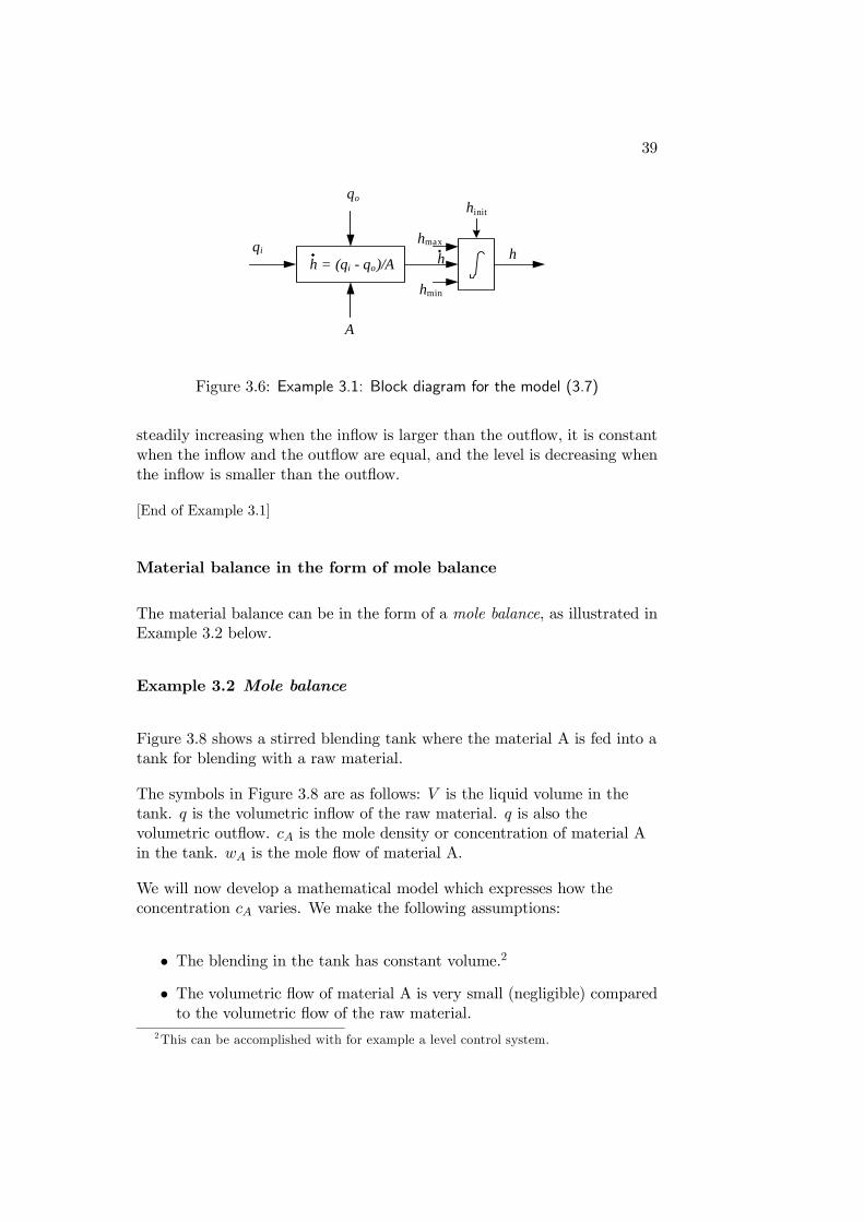
Figure 3.6 shows an alternative mathematical block diagram using aformula block in stead of the elementary blocks. Here, qi enters theformula block at the left because it is a manipulated variable. qo enter theblock at the top because it is an environmental variable, and A enters atthe bottom because it is a parameter.

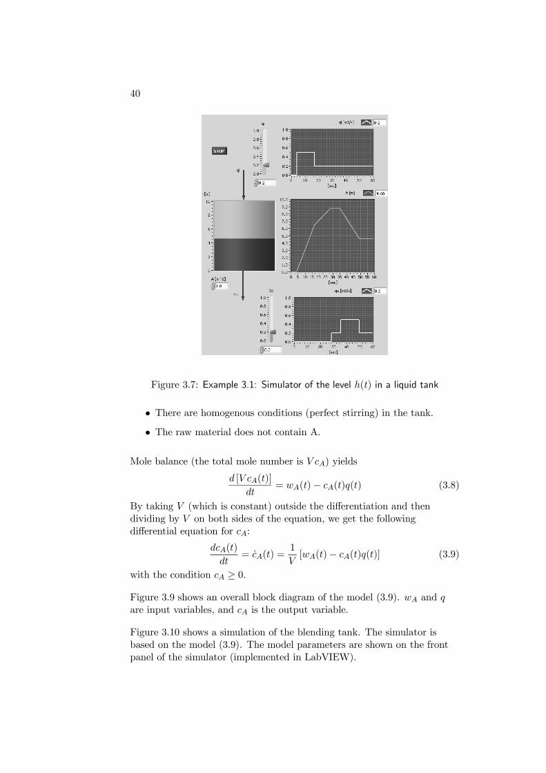
Let us look at a simulation of the tank. The simulator is based on themodel (3.7) and is implemented in LabVIEW. Figure 3.7 shows the inputsignals qi(t) and qo(t) and the corresponding time response in the outputvariable, h(t). The model parameters are shown on the front panel of thesimulator (see the figure). The time response is as expected: The level is

39

hh.

A

hmax

hmin

hinit

qo

qi

h = (qi - qo)/A

Figure 3.6: Example 3.1: Block diagram for the model (3.7)

steadily increasing when the inflow is larger than the outflow, it is constantwhen the inflow and the outflow are equal, and the level is decreasing whenthe inflow is smaller than the outflow.


Material balance in the form of mole balance

The material balance can be in the form of a mole balance, as illustrated inExample 3.2 below.

Example 3.2 Mole balance

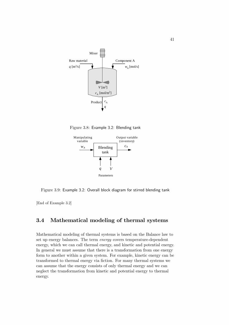
Figure 3.8 shows a stirred blending tank where the material A is fed into atank for blending with a raw material.

The symbols in Figure 3.8 are as follows: V is the liquid volume in thetank. q is the volumetric inflow of the raw material. q is also thevolumetric outflow. cA is the mole density or concentration of material Ain the tank. wA is the mole flow of material A.

We will now develop a mathematical model which expresses how theconcentration cA varies. We make the following assumptions:

• The blending in the tank has constant volume.2

• The volumetric flow of material A is very small (negligible) comparedto the volumetric flow of the raw material.

2This can be accomplished with for example a level control system.

40

Figure 3.7: Example 3.1: Simulator of the level h(t) in a liquid tank

• There are homogenous conditions (perfect stirring) in the tank.

• The raw material does not contain A.

Mole balance (the total mole number is V cA) yields

d [V cA(t)]

dt= wA(t)− cA(t)q(t) (3.8)

By taking V (which is constant) outside the differentiation and thendividing by V on both sides of the equation, we get the followingdifferential equation for cA:

dcA(t)

dt= cA(t) =

1

V[wA(t)− cA(t)q(t)] (3.9)

with the condition cA ≥ 0.

Figure 3.9 shows an overall block diagram of the model (3.9). wA and qare input variables, and cA is the output variable.

Figure 3.10 shows a simulation of the blending tank. The simulator isbased on the model (3.9). The model parameters are shown on the frontpanel of the simulator (implemented in LabVIEW).

41

Mixer

q [m3/s]

Raw material Component A

wA [mol/s]

V [m3]

cA [mol/m3]

Product cA

q

Figure 3.8: Example 3.2: Blending tank

q

Blending tank

cAwA

V


Manipulatingvariable

Parameters

Figure 3.9: Example 3.2: Overall block diagram for stirred blending tank


3.4 Mathematical modeling of thermal systems

Mathematical modeling of thermal systems is based on the Balance law toset up energy balances. The term energy covers temperature-dependentenergy, which we can call thermal energy, and kinetic and potential energy.In general we must assume that there is a transformation from one energyform to another within a given system. For example, kinetic energy can betransformed to thermal energy via fiction. For many thermal systems wecan assume that the energy consists of only thermal energy and we canneglect the transformation from kinetic and potential energy to thermalenergy.

42

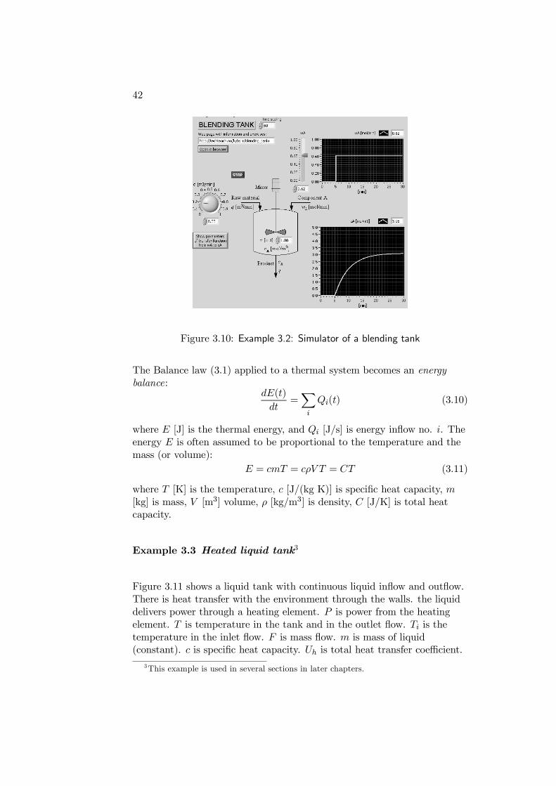
Figure 3.10: Example 3.2: Simulator of a blending tank

The Balance law (3.1) applied to a thermal system becomes an energybalance:

dE(t)

dt=

i

Qi(t) (3.10)

where E [J] is the thermal energy, and Qi [J/s] is energy inflow no. i. Theenergy E is often assumed to be proportional to the temperature and themass (or volume):

E = cmT = cρV T = CT (3.11)

where T [K] is the temperature, c [J/(kg K)] is specific heat capacity, m[kg] is mass, V [m3] volume, ρ [kg/m3] is density, C [J/K] is total heatcapacity.

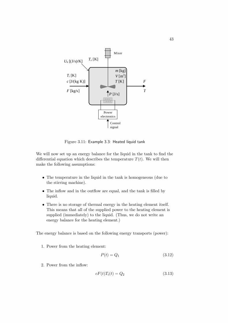
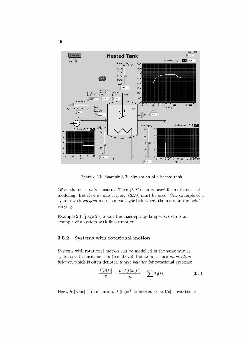
Example 3.3 Heated liquid tank3

Figure 3.11 shows a liquid tank with continuous liquid inflow and outflow.There is heat transfer with the environment through the walls. the liquiddelivers power through a heating element. P is power from the heatingelement. T is temperature in the tank and in the outlet flow. Ti is thetemperature in the inlet flow. F is mass flow. m is mass of liquid(constant). c is specific heat capacity. Uh is total heat transfer coefficient.

3This example is used in several sections in later chapters.

43

c [J/(kg K)]

Ti [K]

F [kg/s]

m [kg]

T [K]

P [J/s]

F

T

Mixer

Te [K]Uh [(J/s)/K]

Powerelectronics

Control signal

V [m3]

Figure 3.11: Example 3.3: Heated liquid tank

We will now set up an energy balance for the liquid in the tank to find thedifferential equation which describes the temperature T (t). We will thenmake the following assumptions:

• The temperature in the liquid in the tank is homogeneous (due tothe stirring machine).

• The inflow and in the outflow are equal, and the tank is filled byliquid.

• There is no storage of thermal energy in the heating element itself.This means that all of the supplied power to the heating element issupplied (immediately) to the liquid. (Thus, we do not write anenergy balance for the heating element.)

The energy balance is based on the following energy transports (power):

1. Power from the heating element:

P (t) = Q1 (3.12)

2. Power from the inflow:

cF (t)Ti(t) = Q2 (3.13)

44

3. Power removed via the outflow:

−cF (t)T (t) = Q3 (3.14)

4. Power via heat transfer from (or to) the environment:

Uh [Te(t)− T (t)] = Q4 (3.15)

The energy balance is

dE(t)

dt= Q1 +Q2 +Q3 +Q4 (3.16)

where the energy is given by

E(t) = cmT (t)

The energy balance can then be written as (here the time argument t isdropped for simplicity):

d (cmT )

dt= P + cFTi − cFT +Uh (Te − T ) (3.17)

If we assume that c and m are constant, we can move cm outside thederivative term. Furthermore, we can combine the the terms on the rightside. The result is

cmdT

dt= cmT = P + cF (Ti − T ) + Uh (Te − T ) (3.18)

which alternatively can be written

dT

dt= T =

1

cm[P + cF (Ti − T ) + Uh (Te − T )] (3.19)

Figure 3.12 shows an overall block diagram of the model (3.19). P and Tiare input variables, and T is an output variable.

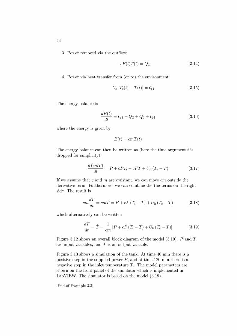
Figure 3.13 shows a simulation of the tank. At time 40 min there is apositive step in the supplied power P , and at time 120 min there is anegative step in the inlet temperature Ti. The model parameters areshown on the front panel of the simulator which is implemented inLabVIEW. The simulator is based on the model (3.19).


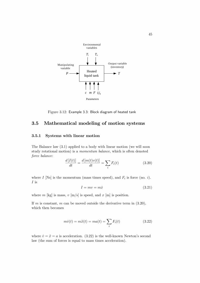
45

PHeated

liquid tankT

Ti Te

c m F Uh

Parameters


Environmentalvariables


Figure 3.12: Example 3.3: Block diagram of heated tank

3.5 Mathematical modeling of motion systems

3.5.1 Systems with linear motion

The Balance law (3.1) applied to a body with linear motion (we will soonstudy rotational motion) is a momentum balance, which is often denotedforce balance:

d [I(t)]

dt=

d [m(t)v(t)]

dt=

i

Fi(t) (3.20)

where I [Ns] is the momentum (mass times speed), and Fi is force (no. i).I is

I = mv =mx (3.21)

where m [kg] is mass, v [m/s] is speed, and x [m] is position.

If m is constant, m can be moved outside the derivative term in (3.20),which then becomes

mv(t) = mx(t) = ma(t) =

i

Fi(t) (3.22)

where v = x = a is acceleration. (3.22) is the well-known Newton’s secondlaw (the sum of forces is equal to mass times acceleration).

46

Figure 3.13: Example 3.3: Simulation of a heated tank

Often the mass m is constant. Then (3.22) can be used for mathematicalmodeling. But if m is time-varying, (3.20) must be used. One example of asystem with varying mass is a conveyor belt where the mass on the belt isvarying.

Example 2.1 (page 25) about the mass-spring-damper system is anexample of a system with linear motion.

3.5.2 Systems with rotational motion

Systems with rotational motion can be modelled in the same way assystems with linear motion (see above), but we must use momentumbalance, which is often denoted torque balance for rotational systems:

d [S(t)]

dt=

d [J(t)ω(t)]

dt=

i

Ti(t) (3.23)

Here, S [Nms] is momentum, J [kgm2] is inertia, ω [rad/s] is rotational

47

speed, and Ti is torque (no. i). If J is constant, (3.23) can be written

Jω(t) = Jθ(t) =

i

Ti(t) (3.24)

where ω = θ is angular acceleration, and θ [rad] is angular position.

Relations between rotational and linear motion

In mathematical modeling of mechanical systems which consists of acombination of rotational and linear systems, the following relations areuseful: Torque T is force F times arm l:

T = Fl (3.25)

Arc b is angle θ (in radians) times radius r:

b = θr (3.26)

Coupled mechanical systems

Mechanical systems often consist of coupled (sub)systems. Each systemcan have linear and/or rotational motion. Some examples: (1) A robotmanipulator where the arms are coupled. (2) A traverse crane where awagon moves a pending load. (3) A motor which moves a load with linearmotion, as in a lathe machine.

A procedure for mathematical modeling of such coupled systems is asfollows:

1. The force or torque balance is put up for each of the (sub)systems,and internal forces and torques acting between the systems aredefined.

2. The final model is derived by eliminating the internal forces andtorques.

This procedure is demonstrated in Example 3.4. An alternative way ofmodeling coupled systems is to use Lagrange mechanics where the model(the equations of motion) are derived from an expression which containskinetic and potential energy for the whole system (this method is notdescribed here).

48

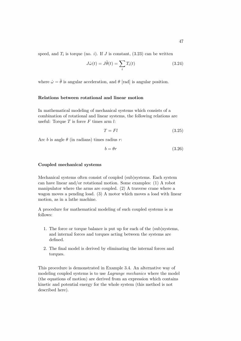
Example 3.4 Modeling coupled rotational and linear motionsystems

Figure 3.14 shows an electro-motor (which can be a current-controlledDC-motor) which moves a load with linear motion via a gear and a rod.

im [A]

Tm = KTim [Nm]

m [kg]

r [m]

[rad]

y [m]0

Rod

Gear

Motor

Load

FL [N]

(radius)

Figure 3.14: Example 3.4: Motor moving a linear load via a gear and a rod

We set up a torque balance for the rotational part of the system and aforce balance for the linear part, and then combines the derived equations.We shall finally have model which expresses the position y of the tool as afunction of the signal i. (For simplicity the time argument t is excluded inthe expressions below.)

1. Torque and force balance: The torque balance for the motorbecomes

Jθ = KT im − T1 (3.27)

where T1 is the torque which acts on the motor from the rod and theload via the gear. The force balance for rod and load becomes

my = F1 − FL (3.28)

where F1 is the force which acts on the rod and the load from themotor via the gear. The relation between T1 and F1 is given by

T1 = F1r (3.29)

49

The relation between y and θ is given by

y = θr (3.30)

which yields

θ =y

r(3.31)

By setting (3.31) and (3.29) into (3.27), (3.27) can be written

Jy

r= KT im − F1r (3.32)

2. Elimination of internal force: By eliminating the internal forceF1 between (3.28) and (3.32), we get

m+

J

r2

y(t) =

KTr

im(t)− FL(t) (3.33)

which is a mathematical model for the coupled system.

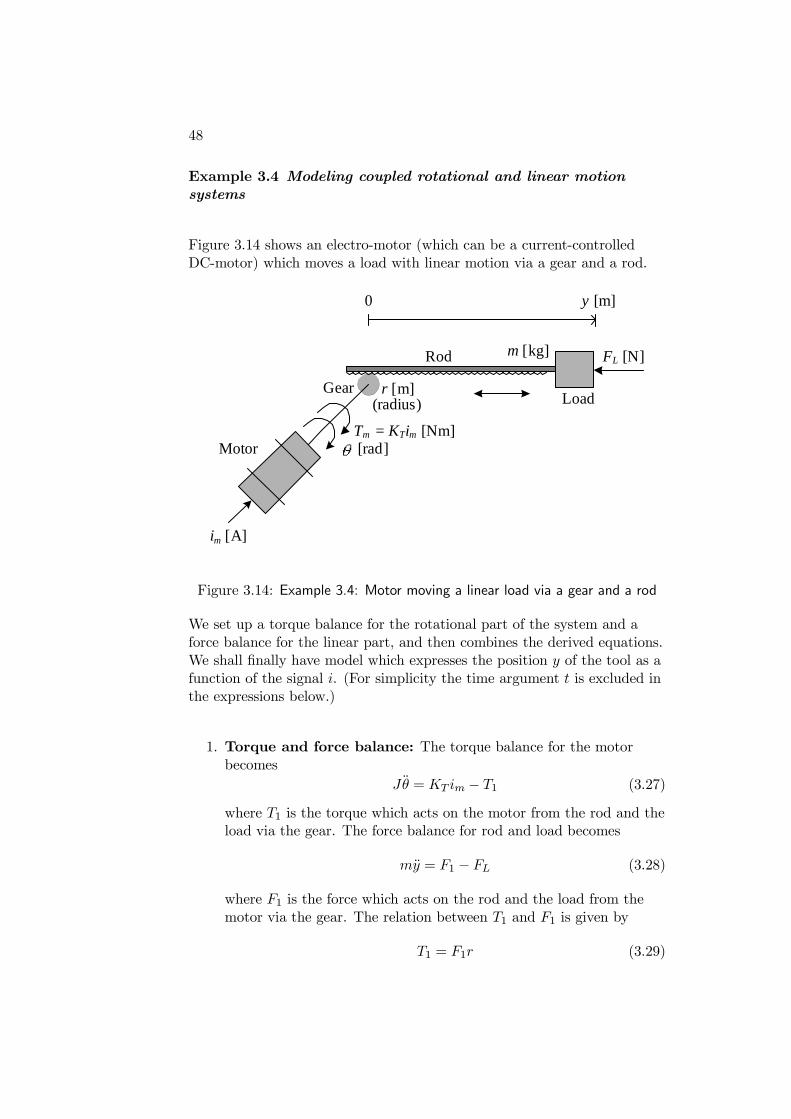
Figure 3.15 shows a block diagram for the model (3.33). im and FL areinput variables, and y is the output variable.

im Motor with rod and load

y

FL

m rJ KT


Environmentalvariable


Parameters

Figure 3.15: Block diagram of motor with rod and load


3.6 Mathematical modeling of electrical systems

Here is a summary of some fundamental formulas for electrical systemswhich you will probably us in mathematical modeling of electrical systems:

50

+

+

+

v2

v3v1

i 2

i3

i1Closedcircuit

Junction

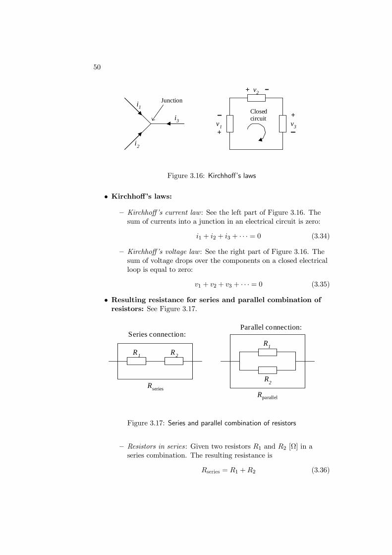
Figure 3.16: Kirchhoff’s laws

• Kirchhoff’s laws:

— Kirchhoff’s current law : See the left part of Figure 3.16. Thesum of currents into a junction in an electrical circuit is zero:

i1 + i2 + i3 + · · · = 0 (3.34)

— Kirchhoff’s voltage law : See the right part of Figure 3.16. Thesum of voltage drops over the components on a closed electricalloop is equal to zero:

v1 + v2 + v3 + · · · = 0 (3.35)

• Resulting resistance for series and parallel combination ofresistors: See Figure 3.17.

R1 R2

R1

R2

Series connection:

RseriesRparallel

Parallel connection:

Figure 3.17: Series and parallel combination of resistors

— Resistors in series: Given two resistors R1 and R2 [Ω] in aseries combination. The resulting resistance is

Rseries = R1 +R2 (3.36)

51

— Resistors in parallel : Given two resistors R1 and R2 [Ω] in aparallel combination. The resulting resistance is

Rparallel =R1 ·R2R1 +R2

(3.37)

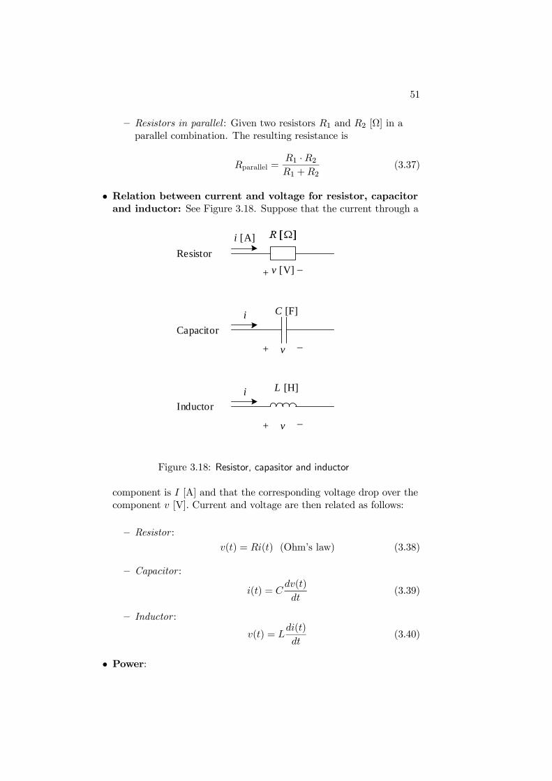
• Relation between current and voltage for resistor, capacitorand inductor: See Figure 3.18. Suppose that the current through a

i [A]

C [F]

+_v [V]

i

+ _v

L [H]i

+ _v

Resistor

Capacitor

Inductor

Figure 3.18: Resistor, capasitor and inductor

component is I [A] and that the corresponding voltage drop over thecomponent v [V]. Current and voltage are then related as follows:

— Resistor :

v(t) = Ri(t) (Ohm’s law) (3.38)

— Capacitor :

i(t) = Cdv(t)

dt(3.39)

— Inductor :

v(t) = Ldi(t)

dt(3.40)

• Power:

52

— Instantaneous power : When a current i flows through a resistorR, the power delivered to the resistor is

P (t) = u(t)i(t) (3.41)

where u(t) = Ri(t) is the voltage drop across the resistor.

— Mean power : When an alternating (sinusoidal) current ofamplitude I flows through a resistor R (for example a heatingelement), the mean or average value of the power delivered tothe resistor is

P =1

2UI =

1

2RI2 =

1

2

U2

R(3.42)

where U is the amplitude of the alternating voltage drop acrossthe resistor. (3.42) is independent of the frequency.

Example 3.5 Mathematical modeling of an RC-circuit

Figure 3.19 shows an RC-circuit (the circuit contains the resistor R andthe capacitor C). The RC-circuit is frequently used as an analog lowpass

vout [V]

++

_ _

vin [V]C [F]

i [A]

Input Output

iC

i2+_

vR [V]

Figure 3.19: RC-circuit

filter: Signals of low frequencies passes approximately unchanged throughthe filter, while signals of high frequencies are approximately filtered out(stopped).

We will now find a mathematical model relating vout to vin. First we applythe Kirchhoff’s voltage law in the circuit which consists the input voltageterminals, the resistor, and the capacitor (we consider the voltage drops tobe positive clockwise direction):

−vin + vR + vout = 0 (3.43)

(vout equals the voltage drop over the capacitor.) In (3.43) vR is given by

vR = Ri (3.44)

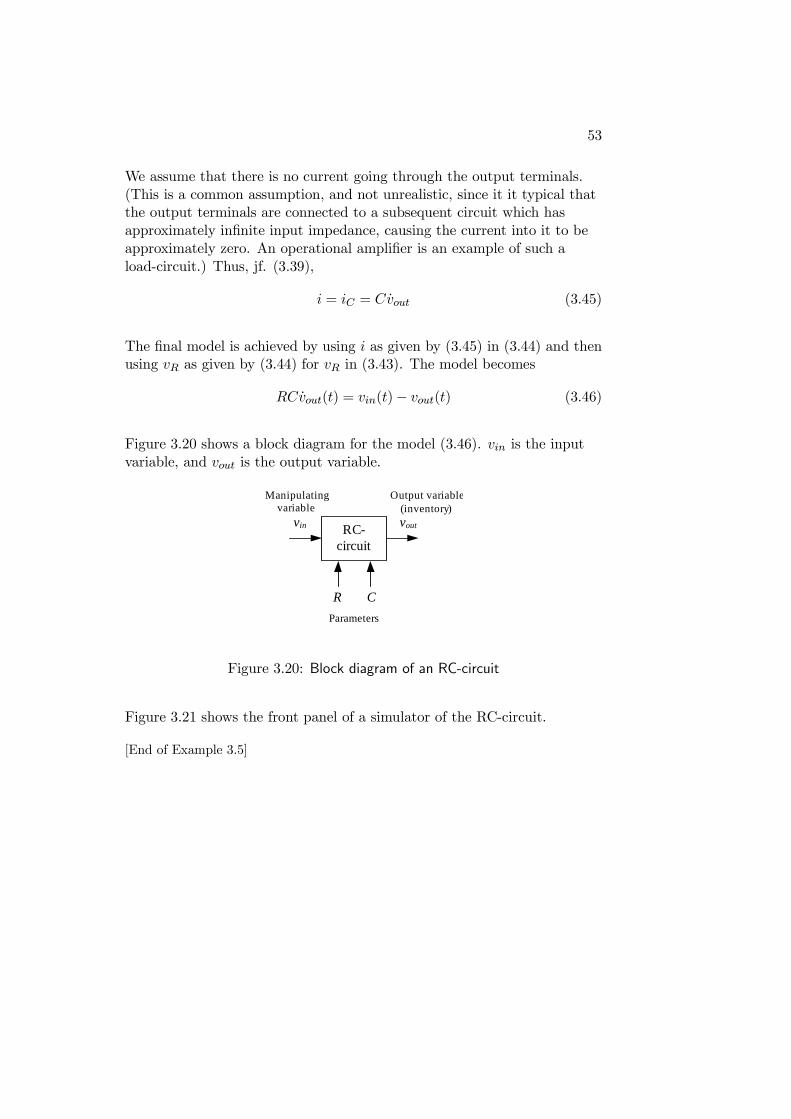
53

We assume that there is no current going through the output terminals.(This is a common assumption, and not unrealistic, since it it typical thatthe output terminals are connected to a subsequent circuit which hasapproximately infinite input impedance, causing the current into it to beapproximately zero. An operational amplifier is an example of such aload-circuit.) Thus, jf. (3.39),

i = iC = Cvout (3.45)

The final model is achieved by using i as given by (3.45) in (3.44) and thenusing vR as given by (3.44) for vR in (3.43). The model becomes

RCvout(t) = vin(t)− vout(t) (3.46)

Figure 3.20 shows a block diagram for the model (3.46). vin is the inputvariable, and vout is the output variable.

vin RC-circuit

vout

R C



Parameters

Figure 3.20: Block diagram of an RC-circuit

Figure 3.21 shows the front panel of a simulator of the RC-circuit.


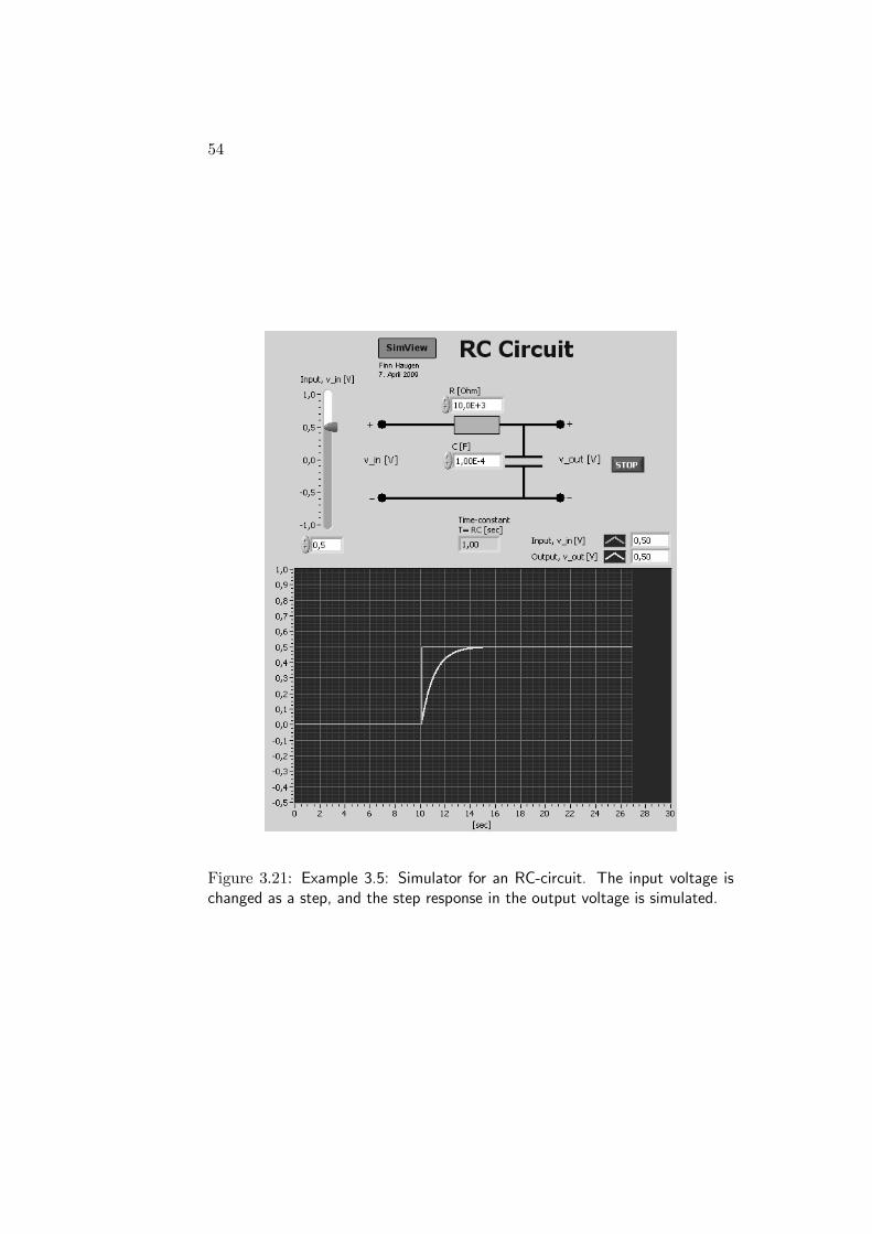
54

Figure 3.21: Example 3.5: Simulator for an RC-circuit. The input voltage ischanged as a step, and the step response in the output voltage is simulated.

Chapter 4

The Laplace transform

4.1 Introduction

The Laplace transform is a mathematical tool which is useful in systemstheory. It is the foundation of transfer functions which is a standard modelform of dynamic systems. Transfer functions are described in Chapter 5.Furthermore, with the Laplace transform you relatively easily calculateresponses in dynamic systems by hand.1

In this chapter I present the Laplace transform at a minimum level. Youcan find much more information in a mathematics text-book.

4.2 Definition of the Laplace transform

Given a time-evaluated function f(t) — that is, f(t) is a function of time t.It can be a sinusoid, a ramp, an impulse, a step, a sum of such functions,or any other function of time. The Laplace transform of f(t) can bedenoted F (s), and is given by the following integral:

F (s) = Lf(t) =

∞

0e−stf(t) dt (4.1)

1 It turns out that we rarely need to perform manual calculations of the responses.When we need to know the responses, it is in most situations more conventient to obtainthem by simulating the system. With the Laplace transform you can calculate responsesonly for linear systems, that is, systems having a model which can be expressed as a lineardifferential equation.

55

56

Expressed with words, f(t) is multiplied by the weight function e−st, andthe resulting product e−stf(t) is integrated from start time t = 0 to endtime t =∞. The Laplace transform does not care about any value thatf(t) might have at negative values of time t. In other words, you can thinkof f(t) as being “switched on” at t = 0. (The so-called two-sided Laplacetransform is defined also for negative time, but it is not relevant for ourapplications.)

s is the Laplace variable.2 F (s) is a function of s. The time t is not avariable in F (s) — it disappeared through the time integration. F (s) willlook completely different from f(t), cf. the following example.

Example 4.1 Laplace transform of a step

Given the function

f(t) = 1 (for t ≥ 0) (4.2)

which is a step of amplitude 1 at time t = 0. Using (4.1), its Laplacetransform becomes

F (s) =

∞

0e−st · 1 · dt =

−1

se−st

t=∞

t=0

=1

s(4.3)


Calculating the time function f(t) from its Laplace transform F (s) — inother words: going from s to t — is denoted inverse Laplace transform.This can be expressed as

f(t) = L−1 F (s) (4.4)

The inverse Laplace transform is actually defined by a complicatedcomplex integral.3 If you really want to calculate this integral, you shoulduse the Residue Theorem in mathematics. However, I suggest you in steadtry the simplest method, namely to find f(t) from the precalculatedLaplace transform pairs, cf. Section 4.3, possibly combined with one ormore of the Laplace transform properties, cf. Section 4.4.

2You may wonder what is the physical meaning of s. It can be interpreted as a complexfrequency, but I think the best answer is that there is no meaningful physical meaning.

3f(t) = 1

2πj

σ+j∞σ−j∞

F (s)estds

57

4.3 Laplace transform pairs

F (s) and f(t) in Example 4.1 can be denoted a Laplace transform pair :

F (s) =1

s⇐⇒ f(t) = 1 (step of amplitude 1) (4.5)

Below are some additional Laplace transform pairs. Each time function,f(t), is defined for t ≥ 0. F (s) can be derived from (4.1). In the expressionsbelow, k is some constant. For example, (4.5) is (4.7) with k = 1.

Laplace transform pairs:

F (s) = k ⇐⇒ f(t) = kδ(t) (impulse of strength or area k) (4.6)

k

s⇐⇒ k (step of amplitude k) (4.7)

k

s2⇐⇒ kt (ramp of slope k) (4.8)

kn!

sn+1⇐⇒ ktn (4.9)

k

Ts+ 1⇐⇒

ke−t/T

T(4.10)

k

(Ts+ 1)s⇐⇒ k

1− e−t/T

(4.11)

k

(T1s+ 1)(T2s+ 1)⇐⇒

k

T1 − T2

e−t/T1 − e−t/T2

(4.12)

k

(T1s+ 1)(T2s+ 1)s⇐⇒ k

1 +

1

T2 − T1

T1e

−t/T1 − T2e−t/T2

(4.13)

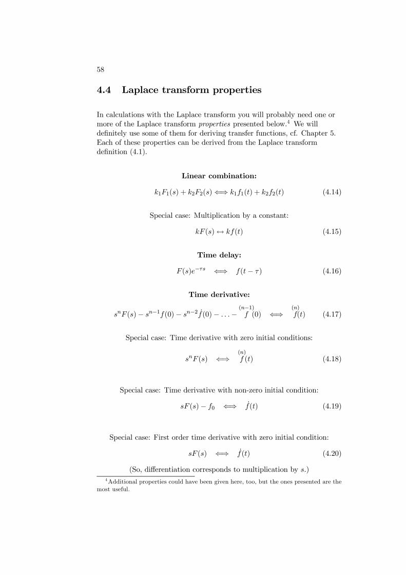
58

4.4 Laplace transform properties

In calculations with the Laplace transform you will probably need one ormore of the Laplace transform properties presented below.4 We willdefinitely use some of them for deriving transfer functions, cf. Chapter 5.Each of these properties can be derived from the Laplace transformdefinition (4.1).

Linear combination:

k1F1(s) + k2F2(s)⇐⇒ k1f1(t) + k2f2(t) (4.14)

Special case: Multiplication by a constant:

kF (s)↔ kf(t) (4.15)

Time delay:

F (s)e−τs ⇐⇒ f(t− τ) (4.16)

Time derivative:

snF (s)− sn−1f(0)− sn−2f(0)− . . .−(n−1)

f (0) ⇐⇒(n)

f(t) (4.17)

Special case: Time derivative with zero initial conditions:

snF (s) ⇐⇒(n)

f (t) (4.18)

Special case: Time derivative with non-zero initial condition:

sF (s)− f0 ⇐⇒ f(t) (4.19)

Special case: First order time derivative with zero initial condition:

sF (s) ⇐⇒ f(t) (4.20)

(So, differentiation corresponds to multiplication by s.)4Additional properties could have been given here, too, but the ones presented are the

most useful.

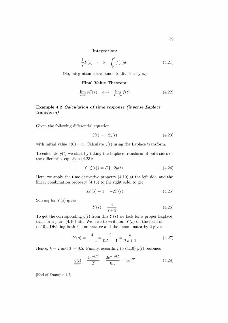
59

Integration:

1

sF (s) ⇐⇒

t

0f(τ)dτ (4.21)

(So, integration corresponds to division by s.)

Final Value Theorem:

lims→0

sF (s) ⇐⇒ limt→∞

f(t) (4.22)

Example 4.2 Calculation of time response (inverse Laplacetransform)

Given the following differential equation:

y(t) = −2y(t) (4.23)

with initial value y(0) = 4. Calculate y(t) using the Laplace transform.

To calculate y(t) we start by taking the Laplace transform of both sides ofthe differential equation (4.23):

Ly(t) = L−2y(t) (4.24)

Here, we apply the time derivative property (4.19) at the left side, and thelinear combination property (4.15) to the right side, to get

sY (s)− 4 = −2Y (s) (4.25)

Solving for Y (s) gives

Y (s) =4

s+ 2(4.26)

To get the corresponding y(t) from this Y (s) we look for a proper Laplacetransform pair. (4.10) fits. We have to write our Y (s) on the form of(4.10). Dividing both the numerator and the denominator by 2 gives

Y (s) =4

s+ 2=

2

0.5s+ 1=

k

Ts+ 1(4.27)

Hence, k = 2 and T = 0.5. Finally, according to (4.10) y(t) becomes

y(t) =ke−t/T

T=2e−t/0.5

0.5= 4e−2t (4.28)


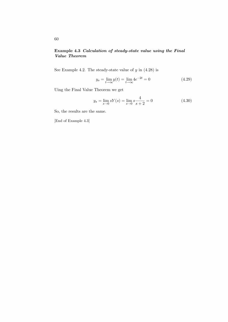
60

Example 4.3 Calculation of steady-state value using the FinalValue Theorem

See Example 4.2. The steady-state value of y in (4.28) is

ys = limt→∞

y(t) = limt→∞

4e−2t = 0 (4.29)

Uing the Final Value Theorem we get

ys = lims→0

sY (s) = lims→0

s4

s+ 2= 0 (4.30)

So, the results are the same.


Chapter 5

Transfer functions

5.1 Introduction

Transfer functions is a model form based on the Laplace transform, cf.Chapter 4. Transfer functions are very useful in analysis and design oflinear dynamic systems, in particular controller functions and signal filters.The main reasons why transfer functions are useful are as follows:

• Compact model form: If the original model is a higher orderdifferential equation, or a set of first order differential equations, therelation between the input variable and the output variable can bedescribed by one transfer function, which is a rational function of theLaplace variable s, without any time-derivatives.

• Representation of standard models: Transfer functions are oftenused to represent standard models of controllers and signal filters.

• Simple to combine systems: For example, the transfer functionfor a combined system which consists of two systems in a seriescombination, is just the product of the transfer functions of eachsystem.

• Simple to calculate time responses: The calculations will bemade using the Laplace transform, and the necessary mathematicaloperations are usually much simpler than solving differentialequations. Calculation of time-responses for transfer function modelsis described in Chapter 5.5.

• Simple to find the frequency response: The frequency responseis a function which expresses how sinusoid signals are transfered

61

62

through a dynamic system. Frequency response is an important toolin analysis and design of signal filters and control systems. Thefrequency response can be found from the transfer function of thesystem. However, frequency response theory is not a part of thisbook (a reference is [2]).

Before we start, I must say something about the mathematical notation:In the following sections, and in the reminder of the book, I use the samesymbol (letter) for the time function, say y(t), as for the Laplace transformof y(t), here y(s) — although it is mathematically incorrect to do it. Thereason is to simplify the presentation. Now, only one variable name(symbol) is needed for both the Laplace domain and the time domain. Forexample, assume that y(t) is the time function of the level y in a watertank. Then I write y(s), although I formally should have written Y (s) ory∗(s) or y(s) (or something else that is different from y(s)) for Ly(t). Itis my experience (from many years together with transfer functions) thatthis simplifying notation causes no problems.

5.2 Definition of the transfer function

The first step in deriving the transfer function of a system is taking theLaplace transform of the differential equation (which must be linear). Letus go on with an example, but the results are general. Given the followingmathematical model having two input variables u1 and u2 and one outputvariable y. (I think you will understand from this example how to find thetransfer function for systems with different number of inputs and outputs.)

y(t) = ay(t) + b1u1(t) + b2u2(t) (5.1)

a, b1 and b2 are model parameters (coefficients). Let the initial state (attime t = 0) be y0. We start by taking the Laplace transform of both sidesof the differential equation:

Ly(t) = Lay(t) + b1u1(t) + b2u2(t) (5.2)

By using the linearity property of the Laplace transform, cf. (4.14), theright side of (5.2) can be written as

Lay(t)+ Lb1u1(t)+ Lb2u2(t) (5.3)

= aLy(t)+ b1Lu1(t)+ b2Lu2(t) (5.4)

= ay(s) + b1u1(s) + b2u2(s) (5.5)

63

The left side of (5.2) will be Laplace transformed using the differentiationrule, cf. (4.17), on Ly(t):

Ly(t) = sy(s)− y0 (5.6)

Thus, we have found that the Laplace transformed (5.2) is

sy(s)− y0 = ay(s) + b1u1(s) + b2u2(s) (5.7)

Solving for the output variable y(s) gives

y(s) =

yin it (s) 1

s− ay0 +

y1(s) b1

s− a H1(s)

u1(s) +

y2(s) b2

s− a H2(s)

u2(s) (5.8)

In (5.8),

• y1 is the contribution from input u1 to the total response y,

• y2 is the contribution from input u2 to the total response y,

• yinit is the contribution from the initial state y0 to the total responsey.

Of course, these contributions to the total response are in the Laplacedomain. The corresponding responses in the time domain are found bycalculating the inverse Laplace transforms.

Now we have the following two transfer functions for our system:

• The transfer function from u1 to y is

H1(s) =b1

s− a(5.9)

• The transfer function from u2 to y is

H2(s) =b2

s− a(5.10)

Thus, the transfer function from a given input variable to a given outputvariable is the s-valued function with which the Laplace transformed inputvariable is multiplied to get its contribution to the response in the output

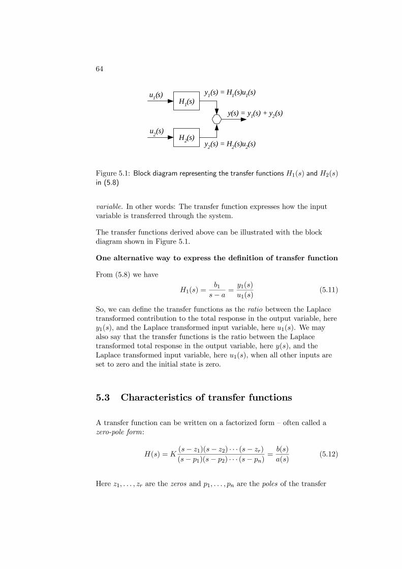
64

H1(s)u1(s)

y(s) = y1(s) + y2(s)

H2(s)

y1(s) = H1(s)u1(s)

y2(s) = H2(s)u2(s)

u2(s)

Figure 5.1: Block diagram representing the transfer functions H1(s) and H2(s)in (5.8)

variable. In other words: The transfer function expresses how the inputvariable is transferred through the system.

The transfer functions derived above can be illustrated with the blockdiagram shown in Figure 5.1.

One alternative way to express the definition of transfer function

From (5.8) we have

H1(s) =b1

s− a=

y1(s)

u1(s)(5.11)

So, we can define the transfer functions as the ratio between the Laplacetransformed contribution to the total response in the output variable, herey1(s), and the Laplace transformed input variable, here u1(s). We mayalso say that the transfer functions is the ratio between the Laplacetransformed total response in the output variable, here y(s), and theLaplace transformed input variable, here u1(s), when all other inputs areset to zero and the initial state is zero.

5.3 Characteristics of transfer functions

A transfer function can be written on a factorized form — often called azero-pole form:

H(s) = K(s− z1)(s− z2) · · · (s− zr)

(s− p1)(s− p2) · · · (s− pn)=

b(s)

a(s)(5.12)

Here z1, . . . , zr are the zeros and p1, . . . , pn are the poles of the transfer

65

function. For example, the transfer function

H(s) =4s− 4

s2 + 5s+ 6= 4

s− 1

(s+ 3)(s+ 2)(5.13)

have two poles, −3 and −2, one zero, 1, and the gain is 4. (As shown ine.g. [2] the values of the poles determines the stability property of asystem. The system is stable only if all the poles have negative real parts,in other words if all the poles lie in the left half part of the complex plane.But we will not go into any stability analysis here.)

The s-polynomial in the denominator of H(s), which is a(s) in (5.12), isdenoted the characteristic polynomial. The poles are the roots of thecharacteristic polynomial, that is

a(s) = 0 for s = s1, s2, ..., sn (the poles) (5.14)

The order of a transfer function is the order of the characteristicpolynomial. For example, the transfer function (5.13) has order 2.

5.4 Combining transfer functions blocks in blockdiagrams

Transfer function blocks may be combined in a block diagram according tothe rules shown in Figure 5.2. One possible purpose of such a combinationis to simplify the block diagram, or to calculate the resulting or overalltransfer function. For example, the combined transfer function of twotransfer functions connected in series is equal to the product of theindividual transfer functions, jc. the Series connection rule in Figure 5.2.

5.5 How to calculate responses from transferfunction models

It is quite easy to calculate responses in transfer function models manually(by hand). Assume given the following transfer function model:

y(s) = H(s)u(s) (5.15)

To calculate the time-response y(t) for a given input signal u(t), we can doas follows:

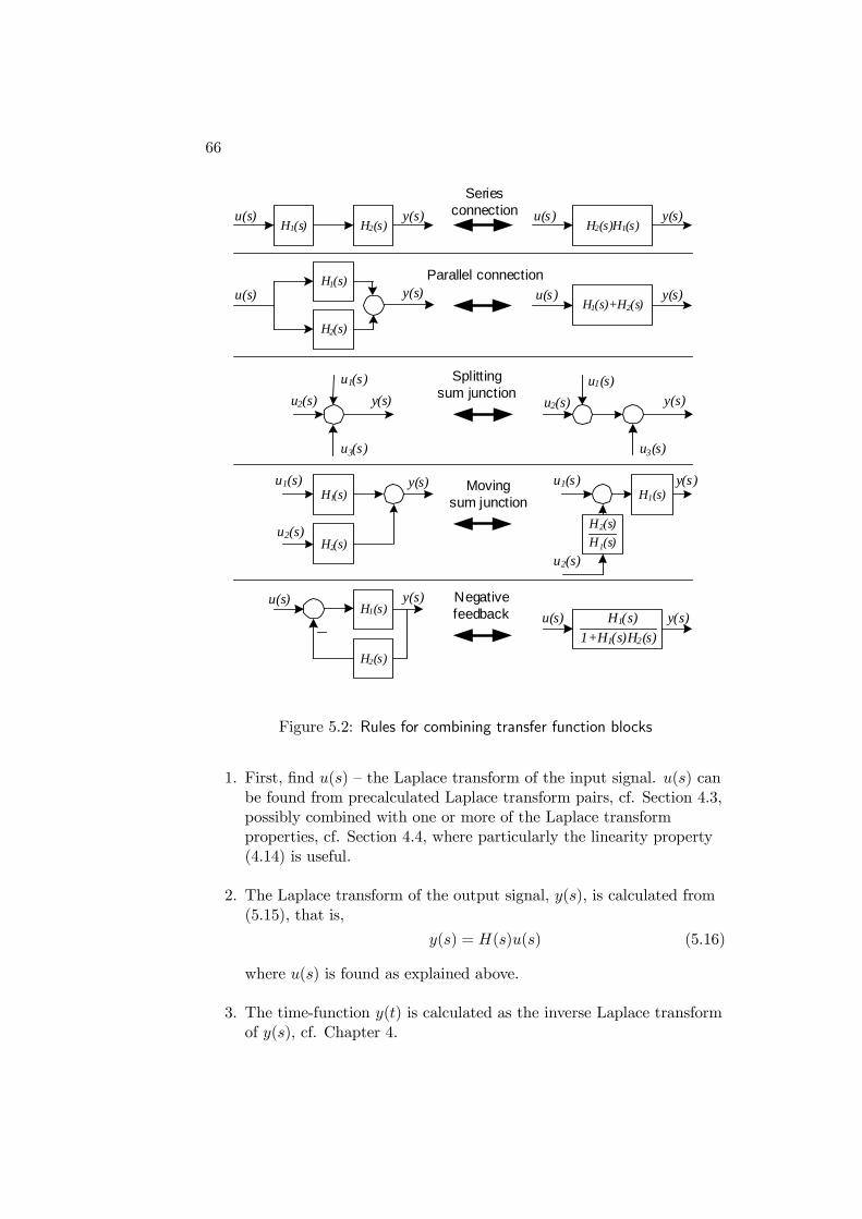
66

H1(s) H2(s) H2(s)H1(s)u(s) u(s)y(s) y(s)

H1(s)

H1(s)+H2(s)u(s) y(s)

Series connection

H2(s)

u(s) y(s)Parallel connection

u1(s)

u2(s)

u3(s)

u1(s)

u2(s)

u3(s)

y(s) y(s)

Splittingsum junction

H1(s)u1(s)

H2(s)u2(s)

y(s) Movingsum junction

H1(s)

u2(s)

u1(s)

H2(s)

H1(s)

y(s)

H1(s)y(s)

H2(s)

Negativefeedback

u(s)H1(s)

1+H1(s)H2(s)

y(s)u(s)

Figure 5.2: Rules for combining transfer function blocks

1. First, find u(s) — the Laplace transform of the input signal. u(s) canbe found from precalculated Laplace transform pairs, cf. Section 4.3,possibly combined with one or more of the Laplace transformproperties, cf. Section 4.4, where particularly the linearity property(4.14) is useful.

2. The Laplace transform of the output signal, y(s), is calculated from(5.15), that is,

y(s) = H(s)u(s) (5.16)

where u(s) is found as explained above.

3. The time-function y(t) is calculated as the inverse Laplace transformof y(s), cf. Chapter 4.

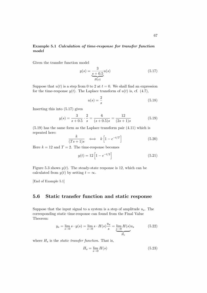
67

Example 5.1 Calculation of time-response for transfer functionmodel

Given the transfer function model

y(s) =3

s+ 0.5 H(s)

u(s) (5.17)

Suppose that u(t) is a step from 0 to 2 at t = 0. We shall find an expressionfor the time-response y(t). The Laplace transform of u(t) is, cf. (4.7),

u(s) =2

s(5.18)

Inserting this into (5.17) gives

y(s) =3

s+ 0.5·2

s=

6

(s+ 0.5)s=

12

(2s+ 1)s(5.19)

(5.19) has the same form as the Laplace transform pair (4.11) which isrepeated here:

k

(Ts+ 1)s⇐⇒ k

1− e−t/T

(5.20)

Here k = 12 and T = 2. The time-response becomes

y(t) = 121− e−t/2

(5.21)

Figure 5.3 shows y(t). The steady-state response is 12, which can becalculated from y(t) by setting t =∞.


5.6 Static transfer function and static response

Suppose that the input signal to a system is a step of amplitude us. Thecorresponding static time-response can found from the Final ValueTheorem:

ys = lims→0

s · y(s) = lims→0

s ·H(s)uss= lims→0

H(s)

Hs

us (5.22)

where Hs is the static transfer function. That is,

Hs = lims→0

H(s) (5.23)

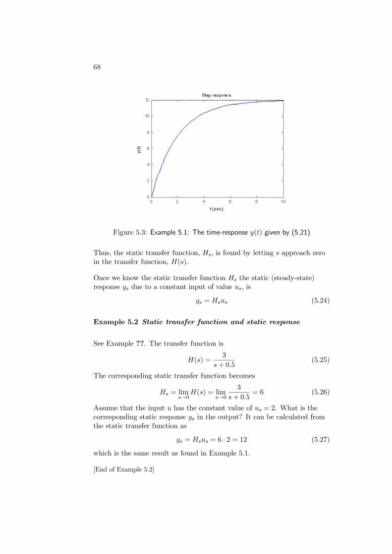
68

Figure 5.3: Example 5.1: The time-response y(t) given by (5.21)

Thus, the static transfer function, Hs, is found by letting s approach zeroin the transfer function, H(s).

Once we know the static transfer function Hs the static (steady-state)response ys due to a constant input of value us, is

ys = Hsus (5.24)

Example 5.2 Static transfer function and static response

See Example ??. The transfer function is

H(s) =3

s+ 0.5(5.25)

The corresponding static transfer function becomes

Hs = lims→0

H(s) = lims→0

3

s+ 0.5= 6 (5.26)

Assume that the input u has the constant value of us = 2. What is thecorresponding static response ys in the output? It can be calculated fromthe static transfer function as

ys = Hsus = 6 · 2 = 12 (5.27)

which is the same result as found in Example 5.1.


Chapter 6

Dynamic characteristics

6.1 Introduction

In this chapter a number of standard dynamic models in the form oftransfer functions will be defined. With such standard models you cancharacterize the dynamic properties of a physical system in terms of forexample gain, time-constant, and time-delay. These terms are also usefulfor controller tuning, as in the Skogestad’s tuning method which isdescribed in Section 10.3.

This chapter covers integrators, time-constant systems and time-delays.Second order systems, which may show oscillatory responses, are notcovered.1

6.2 Integrators

An integrator is a system where the output variable y is the time integralof the input variable u, multiplied with some gain K:

y(t) = K

t

0udθ (6.1)

1Because I have found that the theory about second order systems is not importantin most applications. However, an article about second order systems is available athttp://techteach.no.

69

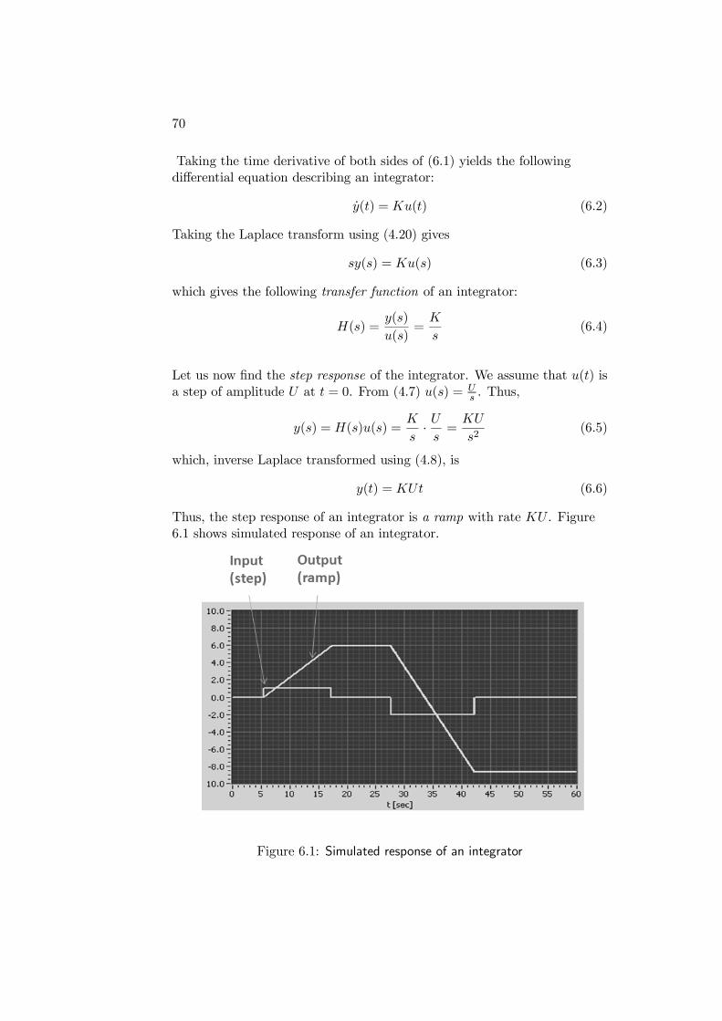
70

Taking the time derivative of both sides of (6.1) yields the followingdifferential equation describing an integrator:

y(t) = Ku(t) (6.2)

Taking the Laplace transform using (4.20) gives

sy(s) = Ku(s) (6.3)

which gives the following transfer function of an integrator:

H(s) =y(s)

u(s)=

K

s(6.4)

Let us now find the step response of the integrator. We assume that u(t) isa step of amplitude U at t = 0. From (4.7) u(s) = U

s . Thus,

y(s) = H(s)u(s) =K

s·U

s=

KU

s2(6.5)

which, inverse Laplace transformed using (4.8), is

y(t) = KUt (6.6)

Thus, the step response of an integrator is a ramp with rate KU . Figure6.1 shows simulated response of an integrator.

Figure 6.1: Simulated response of an integrator

71

Example 6.1 An integrator: A liquid tank

See Example 3.1 on page 36 which describes a liquid tank. Assume forsimplicity that there is no outflow from the tank. The mathematical modelof this system is then

h(t) =1

Aqi(t) (6.7)

Taking the Laplace transform of (6.7) gives

sh(s)− h0 =1

Aqi(s) (6.8)

which gives

h(s) =h0s+

1

AsH(s)

qi(s) (6.9)

So, the transfer function is

H(s) =h(s)

qi(s)=1

A·1

s(6.10)

The system is an integrator!

It is actually quite naturally that the liquid tank is an integrator, since thelevel is proportional to the integral of the inflow. This can be seen byintegrating (6.7), which gives

h(t) = h(0) +

t

0

1

Aqi(θ) dθ (6.11)

Whenever you need a concrete example of an integrator, recall the tank!


6.3 Time-constant systems

In time-constant system — also denoted first order systems — the outputvariable y and the input variable u are related according to the followingdifferential equation:

T y(t) + y(t) = Ku(t) (6.12)

Here K is the gain, and T is the time-constant..

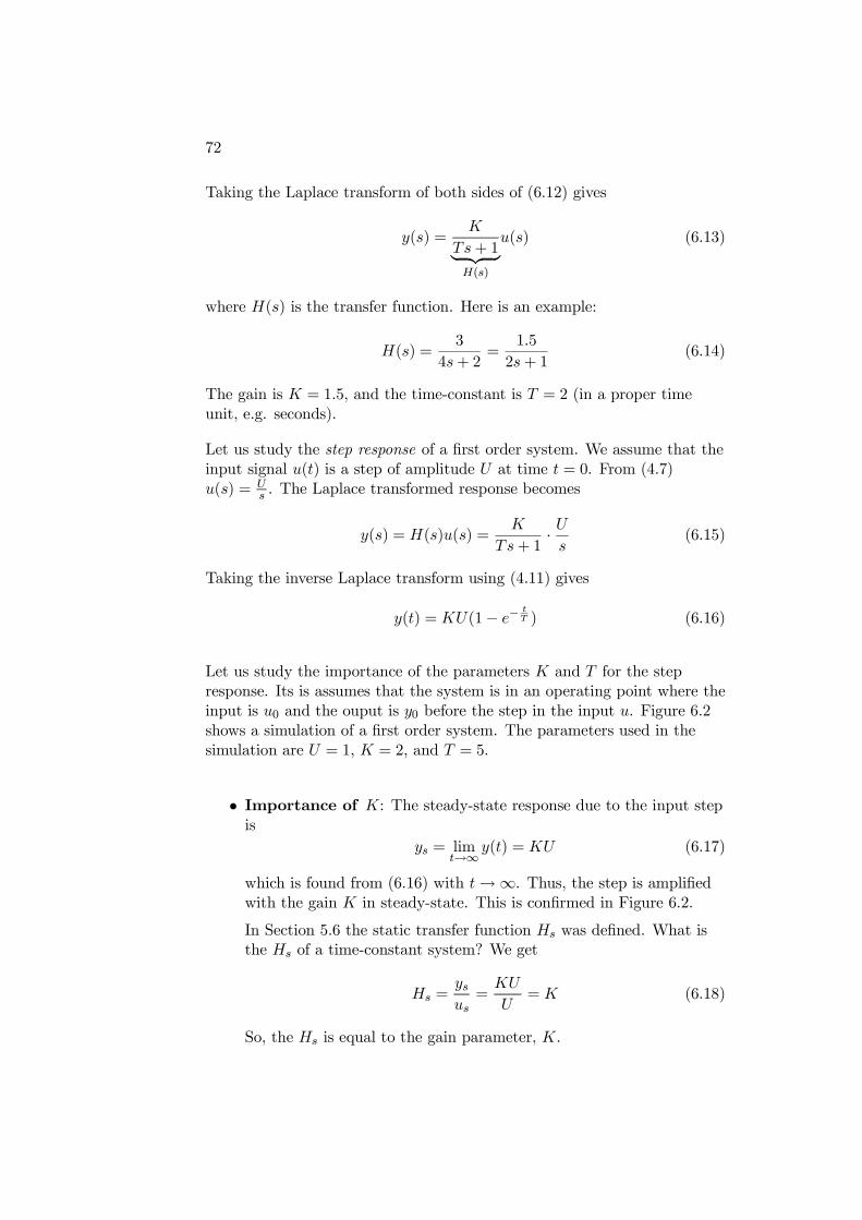
72

Taking the Laplace transform of both sides of (6.12) gives

y(s) =K

Ts+ 1 H(s)

u(s) (6.13)

where H(s) is the transfer function. Here is an example:

H(s) =3

4s+ 2=

1.5

2s+ 1(6.14)

The gain is K = 1.5, and the time-constant is T = 2 (in a proper timeunit, e.g. seconds).

Let us study the step response of a first order system. We assume that theinput signal u(t) is a step of amplitude U at time t = 0. From (4.7)u(s) = U

s . The Laplace transformed response becomes

y(s) = H(s)u(s) =K

Ts+ 1·U

s(6.15)

Taking the inverse Laplace transform using (4.11) gives

y(t) = KU(1− e−tT ) (6.16)

Let us study the importance of the parameters K and T for the stepresponse. Its is assumes that the system is in an operating point where theinput is u0 and the ouput is y0 before the step in the input u. Figure 6.2shows a simulation of a first order system. The parameters used in thesimulation are U = 1, K = 2, and T = 5.

• Importance of K: The steady-state response due to the input stepis

ys = limt→∞

y(t) = KU (6.17)

which is found from (6.16) with t→∞. Thus, the step is amplifiedwith the gain K in steady-state. This is confirmed in Figure 6.2.

In Section 5.6 the static transfer function Hs was defined. What isthe Hs of a time-constant system? We get

Hs =ysus=

KU

U= K (6.18)

So, the Hs is equal to the gain parameter, K.

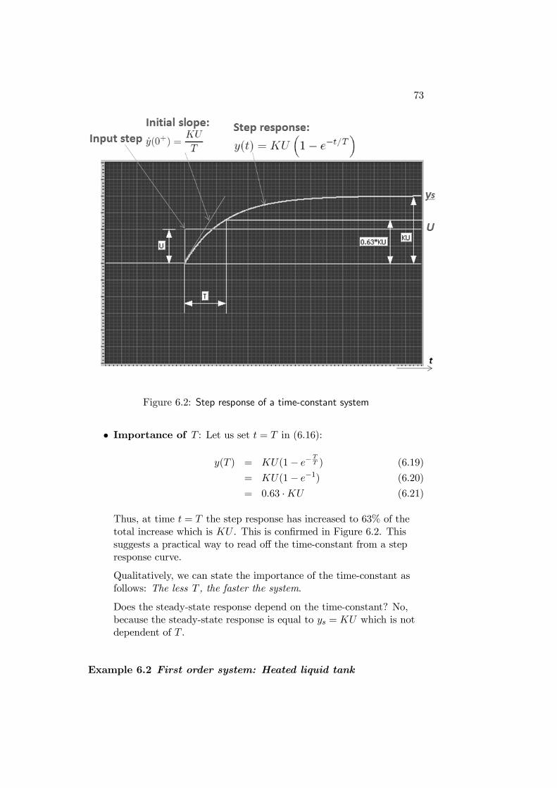
73

Figure 6.2: Step response of a time-constant system

• Importance of T : Let us set t = T in (6.16):

y(T ) = KU(1− e−TT ) (6.19)

= KU(1− e−1) (6.20)

= 0.63 ·KU (6.21)

Thus, at time t = T the step response has increased to 63% of thetotal increase which is KU . This is confirmed in Figure 6.2. Thissuggests a practical way to read off the time-constant from a stepresponse curve.

Qualitatively, we can state the importance of the time-constant asfollows: The less T , the faster the system.

Does the steady-state response depend on the time-constant? No,because the steady-state response is equal to ys = KU which is notdependent of T .

Example 6.2 First order system: Heated liquid tank

74

In Example 3.3 on page 42 we developed a mathematical model of heatedliquid tank (a thermal system). The model is repeated here:

cmT = P + cF (Ti − T ) + Uh(Te − T ) (6.22)

Let’s for simplicity assume that the tank is well isolated so that

Uh ≈ 0 (6.23)

We will now calculate the transfer functions from P to T and from Ti to T .Taking the Laplace transform of (6.22) gives

cm [sT (s)− T0] = P (s) + cF [Ti(s)− T (s)] (6.24)

Since we are to find the transfer function, we may set the initial value tozero:

T0 = 0 (6.25)

From (6.24) we will find

T (s) =K1

T1s+ 1 H1(s)

P (s) +K2

T1s+ 1 H2(s)

Ti(s) (6.26)

The gains and the time-constant of each of the two transfer functions are

K1 =1

cF(6.27)

K2 = 1 (6.28)

T1 =m

F=

MassFlow

(6.29)

Comments:

• The time-constant, which represents the “dynamics”, is the same forboth transfer functions H1(s) and H2(s).

• In many applications the flow F may change. Assume that the flowis decreased. The dynamic properties of the system then change:

— According to (6.27) the gain from P to T increases, and hencethe T becomes more sensitive to P , giving higher value of T fora given change of P .

— According to (6.29) the time-constant increases, causing a moresluggish response in T to a change in P .


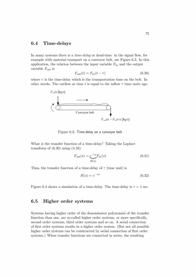
75

6.4 Time-delays

In many systems there is a time-delay or dead-time in the signal flow, forexample with material transport on a conveyor belt, see Figure 6.3. In thisapplication, the relation between the input variable Fin and the outputvariable Fout is

Fout(t) = Fin(t− τ) (6.30)

where τ is the time-delay which is the transportation time on the belt. Inother words: The outflow at time t is equal to the inflow τ time units ago.

Figure 6.3: Time-delay on a conveyor belt

What is the transfer function of a time-delay? Taking the Laplacetransform of (6.30) using (4.16):

Fout(s) = e−τsH(s)

Fin(s) (6.31)

Thus, the transfer function of a time-delay of τ [time unit] is

H(s) = e−τs (6.32)

Figure 6.4 shows a simulation of a time-delay. The time-delay is τ = 1 sec.

6.5 Higher order systems

Systems having higher order of the denominator polynomial of the transferfunction than one, are so-called higher order systems, or more specifically,second order systems, third order systems and so on. A serial connectionof first order systems results in a higher order system. (But not all possiblehigher order systems can be constructed by serial connection of first ordersystems.) When transfer functions are connected in series, the resulting

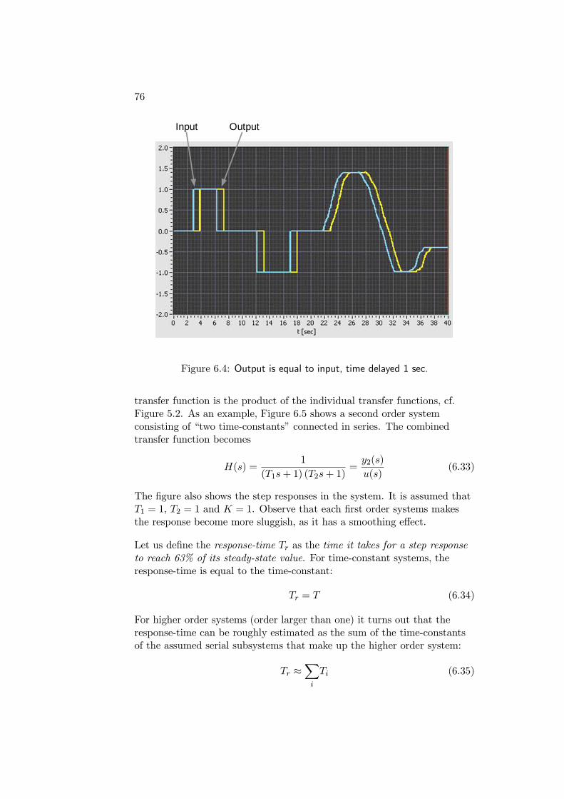
76

Input Output

Figure 6.4: Output is equal to input, time delayed 1 sec.

transfer function is the product of the individual transfer functions, cf.Figure 5.2. As an example, Figure 6.5 shows a second order systemconsisting of “two time-constants” connected in series. The combinedtransfer function becomes

H(s) =1

(T1s+ 1) (T2s+ 1)=

y2(s)

u(s)(6.33)

The figure also shows the step responses in the system. It is assumed thatT1 = 1, T2 = 1 and K = 1. Observe that each first order systems makesthe response become more sluggish, as it has a smoothing effect.

Let us define the response-time Tr as the time it takes for a step responseto reach 63% of its steady-state value. For time-constant systems, theresponse-time is equal to the time-constant:

Tr = T (6.34)

For higher order systems (order larger than one) it turns out that theresponse-time can be roughly estimated as the sum of the time-constantsof the assumed serial subsystems that make up the higher order system:

Tr ≈

i

Ti (6.35)

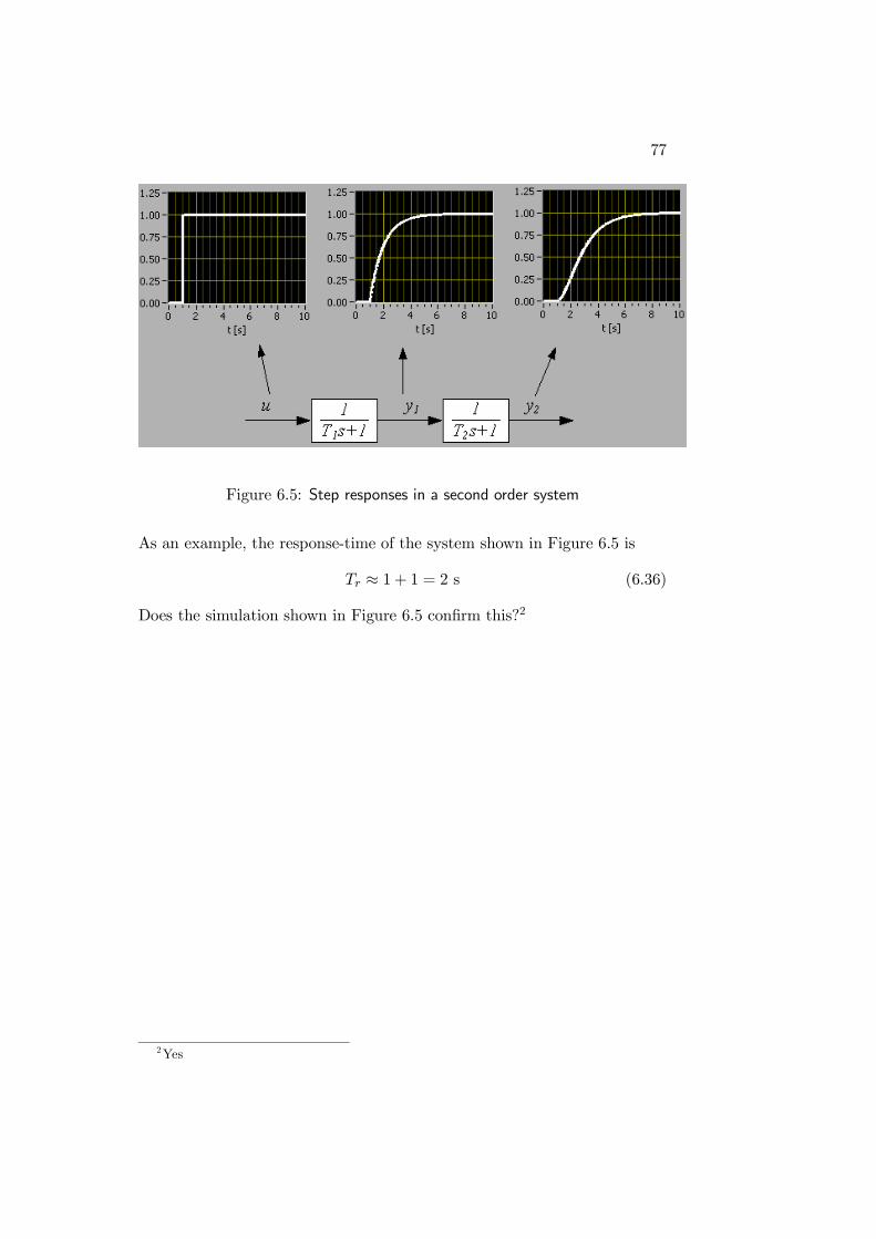
77

Figure 6.5: Step responses in a second order system

As an example, the response-time of the system shown in Figure 6.5 is

Tr ≈ 1 + 1 = 2 s (6.36)

Does the simulation shown in Figure 6.5 confirm this?2

2Yes

Part II

FEEDBACK ANDFEEDFORWARD

CONTROL

79

Chapter 7

Feedback control

7.1 Introduction

The principle of feedback control was introduced back in Section 1.1. Now,we will study feedback control in more detail. The sections which nowfollow continues the description given in Section 1.1.

7.2 Function blocks in the control loop

We will study the function blocks in a typical control loop. If you are tocreate a simulator of a given control system, these blocks must be includedin the simulator (in a simplified simulator you may combine some of theblocks, of course). The level control system for the wood-chip tank, cf.Section 1.2.1, is used as a concrete example.

7.2.1 Automatic and manual mode

Figure 7.1 shows a detailed block diagram of the level control system. Theblock diagram contains a switch between automatic mode and manualmode of the controller. On industrial controllers the operator can switchbetween automatic and manual mode with a button or menu selection onthe user interface (front panel, or screen) of the controller.

• Automatic mode: The controller calculates the control signal usingthe control function (typically a PID control function).

81

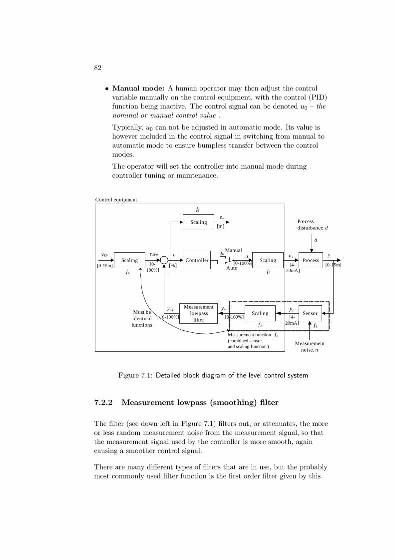
82

• Manual mode: A human operator may then adjust the controlvariable manually on the control equipment, with the control (PID)function being inactive. The control signal can be denoted u0 — thenominal or manual control value .

Typically, u0 can not be adjusted in automatic mode. Its value ishowever included in the control signal in switching from manual toautomatic mode to ensure bumpless transfer between the controlmodes.

The operator will set the controller into manual mode duringcontroller tuning or maintenance.

Process

Sensor

ySPm

d

y

ymf

ScalingySP ue

Controller

Must be identical functions

f4

Scaling

f2 f1

ys

[0-15m] [%]Scaling

f5

u1

Control equipment

Scaling[m]

ey

f6

f3Measurement function (combined sensor and scaling function )

u0

Auto

Manual

Measurementlowpass

filter

Measurementnoise, n

Processdisturbance, d

[0-100%]

ym

[0-100%]

[0-100%] [4-20mA]

[0-15m]

[4-20mA]

[0-100%]

Figure 7.1: Detailed block diagram of the level control system

7.2.2 Measurement lowpass (smoothing) filter

The filter (see down left in Figure 7.1) filters out, or attenuates, the moreor less random measurement noise from the measurement signal, so thatthe measurement signal used by the controller is more smooth, againcausing a smoother control signal.

There are many different types of filters that are in use, but the probablymost commonly used filter function is the first order filter given by this

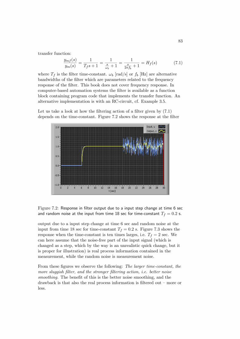
83

transfer function:ymf (s)

ym(s)=

1

Tfs+ 1=

1sωb+ 1

=1

s2πfb

+ 1= Hf (s) (7.1)

where Tf is the filter time-constant. ωb [rad/s] or fb [Hz] are alternativebandwidths of the filter which are parameters related to the frequencyresponse of the filter. This book does not cover frequency response. Incomputer-based automation systems the filter is available as a functionblock containing program code that implements the transfer function. Analternative implementation is with an RC-circuit, cf. Example 3.5.

Let us take a look at how the filtering action of a filter given by (7.1)depends on the time-constant. Figure 7.2 shows the response at the filter

Figure 7.2: Response in filter output due to a input step change at time 6 secand random noise at the input from time 18 sec for time-constant Tf = 0.2 s.

output due to a input step change at time 6 sec and random noise at theinput from time 18 sec for time-constant Tf = 0.2 s. Figure 7.3 shows theresponse when the time-constant is ten times larges, i.e. Tf = 2 sec. Wecan here assume that the noise-free part of the input signal (which ischanged as a step, which by the way is an unrealistic quick change, but itis proper for illustration) is real process information contained in themeasurement, while the random noise is measurement noise.

From these figures we observe the following: The larger time-constant, themore sluggish filter, and the stronger filtering action, i.e. better noisesmoothing. The benefit of this is the better noise smoothing, and thedrawback is that also the real process information is filtered out — more orless.

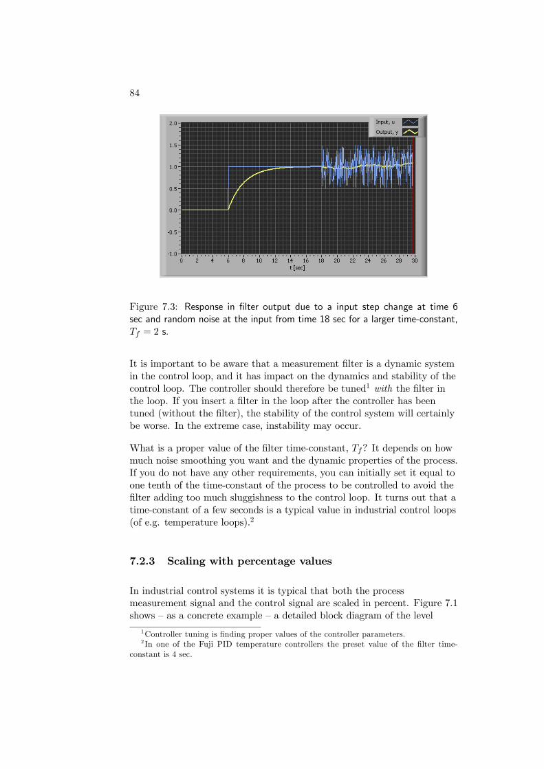
84

Figure 7.3: Response in filter output due to a input step change at time 6sec and random noise at the input from time 18 sec for a larger time-constant,Tf = 2 s.

It is important to be aware that a measurement filter is a dynamic systemin the control loop, and it has impact on the dynamics and stability of thecontrol loop. The controller should therefore be tuned1 with the filter inthe loop. If you insert a filter in the loop after the controller has beentuned (without the filter), the stability of the control system will certainlybe worse. In the extreme case, instability may occur.

What is a proper value of the filter time-constant, Tf? It depends on howmuch noise smoothing you want and the dynamic properties of the process.If you do not have any other requirements, you can initially set it equal toone tenth of the time-constant of the process to be controlled to avoid thefilter adding too much sluggishness to the control loop. It turns out that atime-constant of a few seconds is a typical value in industrial control loops(of e.g. temperature loops).2

7.2.3 Scaling with percentage values

In industrial control systems it is typical that both the processmeasurement signal and the control signal are scaled in percent. Figure 7.1shows — as a concrete example — a detailed block diagram of the level

1Controller tuning is finding proper values of the controller parameters.2 In one of the Fuji PID temperature controllers the preset value of the filter time-

constant is 4 sec.

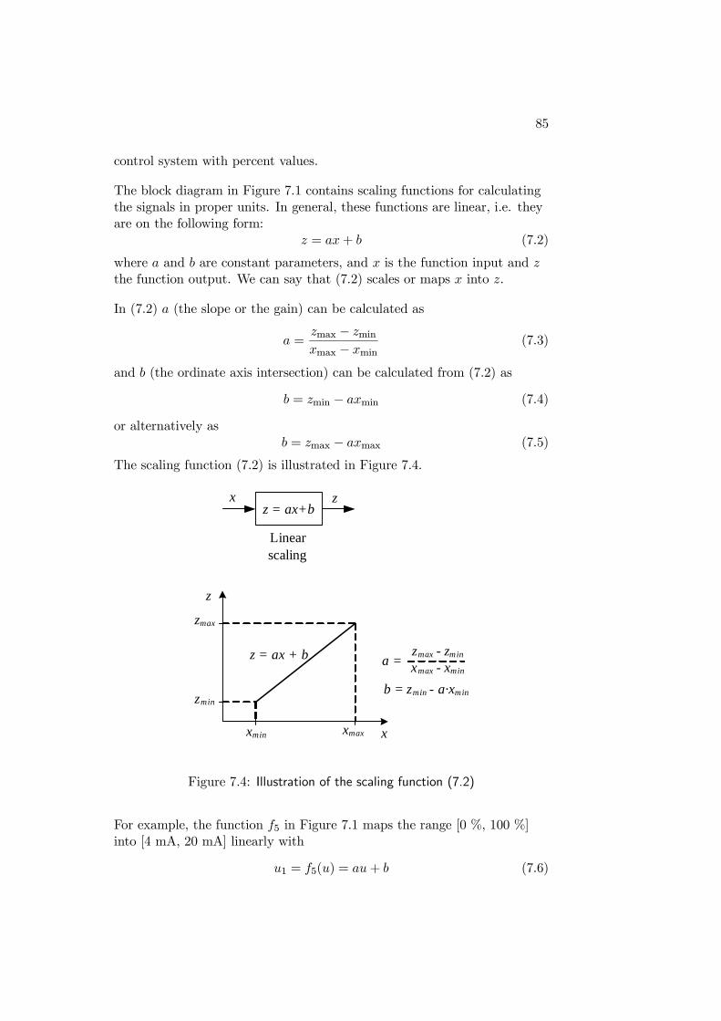
85

control system with percent values.

The block diagram in Figure 7.1 contains scaling functions for calculatingthe signals in proper units. In general, these functions are linear, i.e. theyare on the following form:

z = ax+ b (7.2)

where a and b are constant parameters, and x is the function input and zthe function output. We can say that (7.2) scales or maps x into z.

In (7.2) a (the slope or the gain) can be calculated as

a =zmax − zminxmax − xmin

(7.3)

and b (the ordinate axis intersection) can be calculated from (7.2) as

b = zmin − axmin (7.4)

or alternatively asb = zmax − axmax (7.5)

The scaling function (7.2) is illustrated in Figure 7.4.

z = ax+bzx

Linearscaling

x

z

z = ax + b

xmin xmax

zmax

zmin

a = zmax- zmin

xmax- xmin

b = zmin - a·xmin

Figure 7.4: Illustration of the scaling function (7.2)

For example, the function f5 in Figure 7.1 maps the range [0 %, 100 %]into [4 mA, 20 mA] linearly with

u1 = f5(u) = au+ b (7.6)

86

where

a =u1max − u1minumax − umin

=20mA− 4mA100 %− 0 %

= 0.16 mA/% (7.7)

andb = u1min − aumin = 4mA− a · 0 % = 4mA (7.8)

Let us look at some of the blocks.

• Sensor or measurement function, f1, represents the relationbetween the process output variable y and the physical sensor signalys. For industrial applications a number of standard signal ranges ofmeasurement signals are defined. Common standard ranges are 0—5V, 1—5 V, and 4—20 mA, the latter being the most common.

Wood-chip tank example: The level range [0 m, 15 m] is mapped intoa sensor signal range [4 mA, 20 mA] with a linear relation betweenthe ranges. (Of course this scaling is not implementedmathematically, but is inherent in the sensor.) If you need amathematical function that represents this mapping e.g. in asimulator, you can assume it is on the form (7.2).

• Measurement signal scaling, f2: It is common that the physicalsensor signal is a current between 4 mA and 20 mA, and that theunit of the scaled measurement signal is % (percent). The %-value isthen used in the control function. Commercial control equipmentcontains functions for scaling. During configuration of the controller,the user typically gives information about the minimum and themaximum values of the physical sensor signal, e.g. 4 mA and 20 mA,and the minimum and the maximum values of the scaledmeasurement signal, e.g. 0 % and 100 %. From this information thecontroller automatically configures the scaling function, f2.

Wood-chip tank example: The sensor signal range [4 mA, 20 mA] ismapped linearly into the measurement signal range [0 %, 100 %].The mapping is on the form (7.2).

• Combined measurement scaling and sensor function: Thefunction f3 in Figure 7.1 is the combined function of the sensor andthe subsequent scaling.

Wood-chip tank example: The level range [0 m, 15 m] is mappedlinearly into the measurement signal range [0 %, 100 %]. Themapping is on the form (7.2).

• Setpoint scaling, f4: The setpoint and the measurement signalmust be represented with the same engineering unit, otherwise

87

subtracting the measurement signal from the setpoint is meaningless.The setpoint scaling must be the same as the combined measurementscaling and sensor function, f3.

Wood-chip tank example: The level setpoint range [0 m, 15 m] ismapped linearly into the setpoint range [0 %, 100 %]. The mappingis on the form (7.2).

• Control variable scaling, f5: If the controller calculates thecontrol variable u in % (which is quite common), then a scaling ofthe %-value to the physical unit used by the actuator, is necessary.

Wood-chip tank example: The control signal range [0 %, 100 %] ismapped linearly into the range [4 mA, 20 mA], cf. (7.6).

• Control error scaling, f6: The control error being used as theinput to the controller function is commonly in unit %. If you needto map this percentage value into a physical engineering unit, alinear function on the form (7.6) can be used, but the parameter bwill be zero.

Wood-chip tank example: The control error range [—100 %, 100 %] ismapped linearly into the range [—15 m, 15 m]. The mapping is on theform (7.2).

• Unit of the controller gain: It may be useful, e.g. in controllertuning, to be aware the unit of the (PID) controller gain. Thegeneral formula of the controller gain is as follows:

Unit of controller gain (Kp) =Unit of control signal (u)

Unit of measurement signal (ymf )(7.9)

Assume that both the unit of the control signal and of themeasurement signal have unit of percent. Then the unit of controllergain (Kp) becomes %/% = 1.

7.2.4 Scaling with physical (engineering) values

The control loop will contain fewer blocks if you scale the processmeasurement signal and the control signal in physical (engineering) unitsin stead of in percent. Because the system will appear simpler, you maywant to use physical scaling in stead of percent scaling unless there areimportant reasons for using percent scaling.3

3When I construct control systems from scratch I use physical scaling.

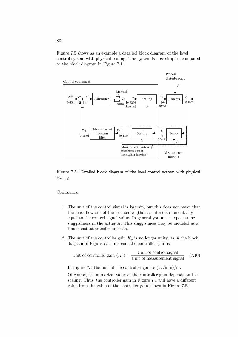
88

Figure 7.5 shows as an example a detailed block diagram of the levelcontrol system with physical scaling. The system is now simpler, comparedto the block diagram in Figure 7.1.

Process

Sensor

d

y

ymf

ySP ueController

Scaling

f2 f1

ys

[0-15m] [m]Scaling

f3

u1

Control equipment

f3Measurement function (combined sensor and scaling function )

u0

Auto

Manual

Measurementlowpass

filter

Measurementnoise, n

Processdisturbance, d

[0-15m]

ym

[0-15m]

[0-3336kg/min]

[4-20mA]

[0-15m]

[4-20mA]

Figure 7.5: Detailed block diagram of the level control system with physicalscaling

Comments:

1. The unit of the control signal is kg/min, but this does not mean thatthe mass flow out of the feed screw (the actuator) is momentarilyequal to the control signal value. In general you must expect somesluggishness in the actuator. This sluggishness may be modeled as atime-constant transfer function.

2. The unit of the controller gain Kp is no longer unity, as in the blockdiagram in Figure 7.1. In stead, the controller gain is

Unit of controller gain (Kp) =Unit of control signal

Unit of measurement signal(7.10)

In Figure 7.5 the unit of the controller gain is (kg/min)/m.

Of course, the numerical value of the controller gain depends on thescaling. Thus, the controller gain in Figure 7.1 will have a differentvalue from the value of the controller gain shown in Figure 7.5.

89

7.3 The PID controller

7.3.1 The ideal PID controller function

Figure 7.1 shows where the control function — usually denoted simply “thecontroller” — is placed in a control loop. The PID controller is thestandard controller function in industry. The ideal PID controller is asfollows (some important modifications are described below):

u = u0 +Kpeup

+Kp

Ti

t

0e dτ

ui

+KpTdde

dt ud

(7.11)

The controller parameters are as follows:

• Kp is the proportional gain. (Other symbols of this gain are Kc (c forcontroller) and K.)

• Ti [s] or [min] is the integral time. In some controllers the value of1/Ti is used in stead of the value of Ti. The unit of 1/Ti is repeatsper minute. For example, 5 repeats per minute means that Ti isequal to 1/5 = 0.2 min.4

• Td [s] or [min] is the derivative time.

• u0 is the nominal value of the control variable. It is the control signalavailable for adjusted by the operator while the controller is inmanual mode. While the controller is in automatic mode, u0 canusually not be adjusted.

In (7.11) up is the P-term. ui is the I-term. ud is the D-term.

In some commercial controllers the proportional band PB, is used in steadof the proportional gain, Kp. The proportional band is given by

PB =100%

Kp(7.12)

where Kp is the gain, which here is assumed to be dimensionless. (It willbe dimensionless if the control error e and the control variable u have the

4The background of the term repeats per minute is as follows: Assume that the controlerror e is constant, say E. The P-term has value up = KpE. During a time interval of 1minute the I-term equals Kp

Ti

1

0E dτ = KpE · 1[min]/Ti = up · 1/Ti. Thus, the I-term has

repeated the P-term 1/Ti times.

90

same unit, typically percent). It is typical that PB has a value in the rangeof 10% ≤ PB ≤ 500%, which corresponds to Kp being in the range of 0.2 ≤Kp ≤ 10. It is important to note that PB is inversely proportional to Kp.Thus, a small PB corresponds to a large Kp, and vice versa.5

The P controller and the PI controller are special cases of the PIDcontroller:

• A P controller is achieved by setting Ti =∞ (or to a very largevalue) and Td = 0.6

• A PI controller is achieved by setting Td = 0.

7.3.2 How the PID controller works

The integral term

The integral term of the PID controller is essential. The I-term is

ui =KpTi

t

0e dτ (7.13)

as calculated as the time integral of the control error e from as initial time,say t = 0, to the present point of time, thus the integral is being calculatedcontinuously. Let us think about the level control of the wood-chip tank.Review Figure 1.3. Assume that e initially is greater than zero (the level isthen less than the level setpoint). As long as e is positive, ui and thereforethe total control variable u will get a steadily increasing value, since thetime integral of a positive value increases with time. The increasing u givesan increasing wood-chip inflow. Consequently, the chip level in the tankincreases. Due to this level increase the control error eventually becomesless positive. The increase of the integral term (the inflow) continues untilthe error has become zero. The conclusion is that the integral term ensureszero steady-state control error. This is illustrated in Figure 7.6.

5What does proportional band actually mean? One explanation is that PB is the changeof the control error interval ∆e (or the size of the measurement signal interval) which givesa change of the control signal interval ∆u equal to 100% (i.e. a full range change of u):From the P-term u = Kpe we see that ∆e = ∆u/Kp = 100%/Kp = PB.

6 In some commercial controllers you can set Ti to 0 (zero), which is a code expressingthat the integral term is de-activated.

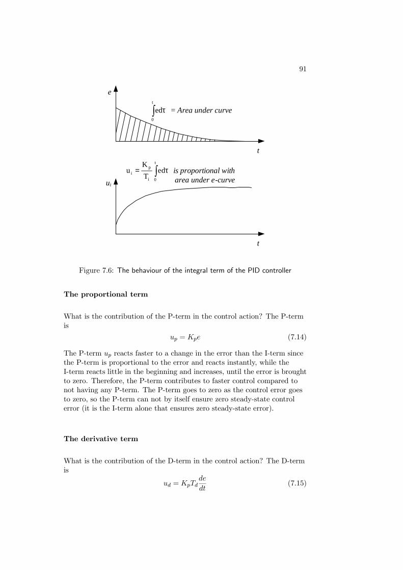
91

t

ui

= Area under curve∫ τt

0

ed

∫ τ=t

0i

pi ed

T

Ku is proportional with

area under e-curve

e

t

Figure 7.6: The behaviour of the integral term of the PID controller

The proportional term

What is the contribution of the P-term in the control action? The P-termis

up = Kpe (7.14)

The P-term up reacts faster to a change in the error than the I-term sincethe P-term is proportional to the error and reacts instantly, while theI-term reacts little in the beginning and increases, until the error is broughtto zero. Therefore, the P-term contributes to faster control compared tonot having any P-term. The P-term goes to zero as the control error goesto zero, so the P-term can not by itself ensure zero steady-state controlerror (it is the I-term alone that ensures zero steady-state error).

The derivative term

What is the contribution of the D-term in the control action? The D-termis

ud = KpTdde

dt(7.15)

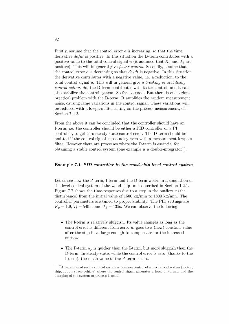
92

Firstly, assume that the control error e is increasing, so that the timederivative de/dt is positive. In this situation the D-term contributes with apositive value to the total control signal u (it assumed that Kp and Td arepositive). This will in general give faster control. Secondly, assume thatthe control error e is decreasing so that de/dt is negative. In this situationthe derivative contributes with a negative value, i.e. a reduction, to thetotal control signal u. This will in general give a breaking or stabilizingcontrol action. So, the D-term contributes with faster control, and it canalso stabilize the control system. So far, so good. But there is one seriouspractical problem with the D-term: It amplifies the random measurementnoise, causing large variations in the control signal. These variations willbe reduced with a lowpass filter acting on the process measurement, cf.Section 7.2.2.

From the above it can be concluded that the controller should have anI-term, i.e. the controller should be either a PID controller or a PIcontroller, to get zero steady-state control error. The D-term should beomitted if the control signal is too noisy even with a measurement lowpassfilter. However there are processes where the D-term is essential forobtaining a stable control system (one example is a double-integrator7).

Example 7.1 PID controller in the wood-chip level control system

Let us see how the P-term, I-term and the D-term works in a simulation ofthe level control system of the wood-chip tank described in Section 1.2.1.Figure 7.7 shows the time-responses due to a step in the outflow v (thedisturbance) from the initial value of 1500 kg/min to 1800 kg/min. Thecontroller parameters are tuned to proper stability. The PID settings areKp = 1.9, Ti = 540 s, and Td = 135s. We can observe the following:

• The I-term is relatively sluggish. Its value changes as long as thecontrol error is different from zero. ui goes to a (new) constant valueafter the step in v, large enough to compensate for the increasedoutflow.

• The P-term up is quicker than the I-term, but more sluggish than theD-term. In steady-state, while the control error is zero (thanks to theI-term), the mean value of the P-term is zero.

7An example of such a control system is position control of a mechanical system (motor,ship, robot, space-vehicle) where the control signal generates a force or torque, and thedamping of the system or process is small.

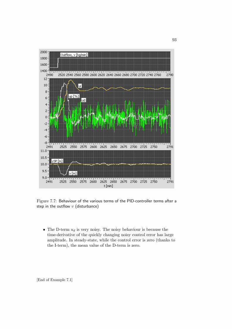
93

Figure 7.7: Behaviour of the various terms of the PID-controller terms after astep in the outflow v (disturbance)

• The D-term ud is very noisy. The noisy behaviour is because thetime-derivative of the quickly changing noisy control error has largeamplitude. In steady-state, while the control error is zero (thanks tothe I-term), the mean value of the D-term is zero.


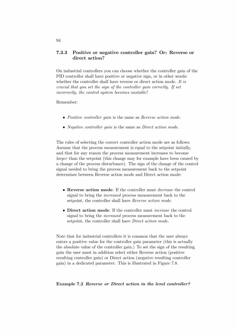
94

7.3.3 Positive or negative controller gain? Or: Reverse ordirect action?

On industrial controllers you can choose whether the controller gain of thePID controller shall have positive or negative sign, or in other words:whether the controller shall have reverse or direct action mode. It iscrucial that you set the sign of the controller gain correctly. If setincorrectly, the control system becomes unstable!

Remember:

• Positive controller gain is the same as Reverse action mode.

• Negative controller gain is the same as Direct action mode.

The rules of selecting the correct controller action mode are as follows.Assume that the process measurement is equal to the setpoint initially,and that for any reason the process measurement increases to becomelarger than the setpoint (this change may for example have been caused bya change of the process disturbance). The sign of the change of the controlsignal needed to bring the process measurement back to the setpointdetermines between Reverse action mode and Direct action mode:

• Reverse action mode: If the controller must decrease the controlsignal to bring the increased process measurement back to thesetpoint, the controller shall have Reverse action mode.

• Direct action mode: If the controller must increase the controlsignal to bring the increased process measurement back to thesetpoint, the controller shall have Direct action mode.

Note that for industrial controllers it is common that the user alwaysenters a positive value for the controller gain parameter (this is actuallythe absolute value of the controller gain.) To set the sign of the resultinggain the user must in addition select either Reverse action (positiveresulting controller gain) or Direct action (negative resulting controllergain) in a dedicated parameter. This is illustrated in Figure 7.8.

Example 7.2 Reverse or Direct action in the level controller?

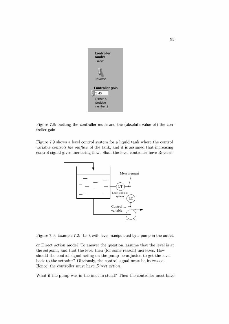
95

Figure 7.8: Setting the controller mode and the (absolute value of) the con-troller gain

Figure 7.9 shows a level control system for a liquid tank where the controlvariable controls the outflow of the tank, and it is assumed that increasingcontrol signal gives increasing flow. Shall the level controller have Reverse

LT

LC

Controlvariable

Measurement

Level controlsystem

Figure 7.9: Example 7.2: Tank with level manipulated by a pump in the outlet.

or Direct action mode? To answer the question, assume that the level is atthe setpoint, and that the level then (for some reason) increases. Howshould the control signal acting on the pump be adjusted to get the levelback to the setpoint? Obviously, the control signal must be increased.Hence, the controller must have Direct action.

What if the pump was in the inlet in stead? Then the controller must have

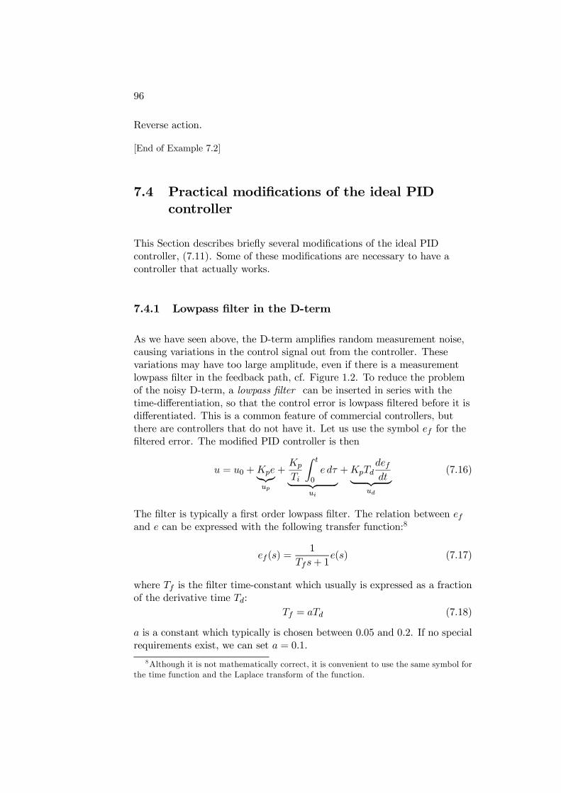
96

Reverse action.


7.4 Practical modifications of the ideal PIDcontroller

This Section describes briefly several modifications of the ideal PIDcontroller, (7.11). Some of these modifications are necessary to have acontroller that actually works.

7.4.1 Lowpass filter in the D-term

As we have seen above, the D-term amplifies random measurement noise,causing variations in the control signal out from the controller. Thesevariations may have too large amplitude, even if there is a measurementlowpass filter in the feedback path, cf. Figure 1.2. To reduce the problemof the noisy D-term, a lowpass filter can be inserted in series with thetime-differentiation, so that the control error is lowpass filtered before it isdifferentiated. This is a common feature of commercial controllers, butthere are controllers that do not have it. Let us use the symbol ef for thefiltered error. The modified PID controller is then

u = u0 +Kpeup

+Kp

Ti

t

0e dτ

ui

+KpTddefdt

ud

(7.16)

The filter is typically a first order lowpass filter. The relation between efand e can be expressed with the following transfer function:8

ef (s) =1

Tfs+ 1e(s) (7.17)

where Tf is the filter time-constant which usually is expressed as a fractionof the derivative time Td:

Tf = aTd (7.18)

a is a constant which typically is chosen between 0.05 and 0.2. If no specialrequirements exist, we can set a = 0.1.

8Although it is not mathematically correct, it is convenient to use the same symbol forthe time function and the Laplace transform of the function.

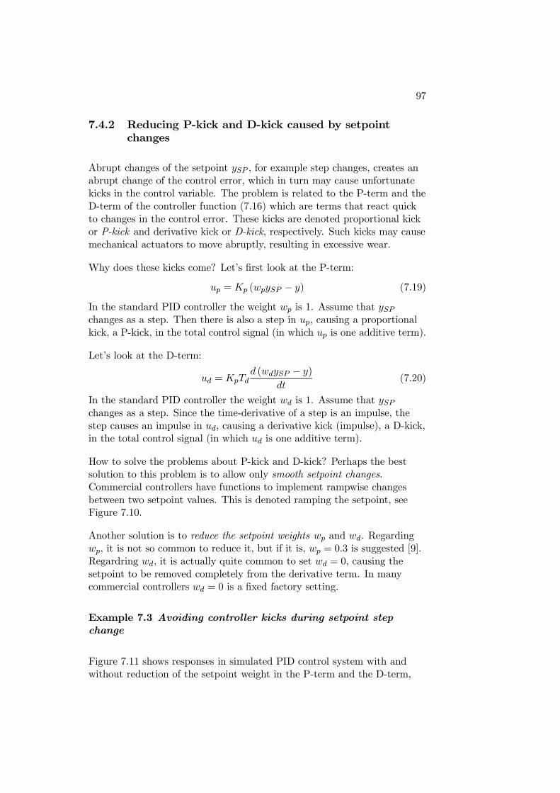
97

7.4.2 Reducing P-kick and D-kick caused by setpointchanges

Abrupt changes of the setpoint ySP , for example step changes, creates anabrupt change of the control error, which in turn may cause unfortunatekicks in the control variable. The problem is related to the P-term and theD-term of the controller function (7.16) which are terms that react quickto changes in the control error. These kicks are denoted proportional kickor P-kick and derivative kick or D-kick, respectively. Such kicks may causemechanical actuators to move abruptly, resulting in excessive wear.

Why does these kicks come? Let’s first look at the P-term:

up = Kp (wpySP − y) (7.19)

In the standard PID controller the weight wp is 1. Assume that ySPchanges as a step. Then there is also a step in up, causing a proportionalkick, a P-kick, in the total control signal (in which up is one additive term).

Let’s look at the D-term:

ud = KpTdd (wdySP − y)

dt(7.20)

In the standard PID controller the weight wd is 1. Assume that ySPchanges as a step. Since the time-derivative of a step is an impulse, thestep causes an impulse in ud, causing a derivative kick (impulse), a D-kick,in the total control signal (in which ud is one additive term).

How to solve the problems about P-kick and D-kick? Perhaps the bestsolution to this problem is to allow only smooth setpoint changes.Commercial controllers have functions to implement rampwise changesbetween two setpoint values. This is denoted ramping the setpoint, seeFigure 7.10.

Another solution is to reduce the setpoint weights wp and wd. Regardingwp, it is not so common to reduce it, but if it is, wp = 0.3 is suggested [9].Regardring wd, it is actually quite common to set wd = 0, causing thesetpoint to be removed completely from the derivative term. In manycommercial controllers wd = 0 is a fixed factory setting.

Example 7.3 Avoiding controller kicks during setpoint stepchange

Figure 7.11 shows responses in simulated PID control system with andwithout reduction of the setpoint weight in the P-term and the D-term,

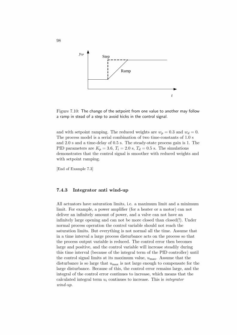
98

t

ySP

Ramp

Step

Figure 7.10: The change of the setpoint from one value to another may followa ramp in stead of a step to avoid kicks in the control signal.

and with setpoint ramping. The reduced weights are wp = 0.3 and wd = 0.The process model is a serial combination of two time-constants of 1.0 sand 2.0 s and a time-delay of 0.5 s. The steady-state process gain is 1. ThePID parameters are Kp = 3.6, Ti = 2.0 s, Td = 0.5 s. The simulationsdemonstrates that the control signal is smoother with reduced weights andwith setpoint ramping.


7.4.3 Integrator anti wind-up

All actuators have saturation limits, i.e. a maximum limit and a minimumlimit. For example, a power amplifier (for a heater or a motor) can notdeliver an infinitely amount of power, and a valve can not have aninfinitely large opening and can not be more closed than closed(!). Undernormal process operation the control variable should not reach thesaturation limits. But everything is not normal all the time. Assume thatin a time interval a large process disturbance acts on the process so thatthe process output variable is reduced. The control error then becomeslarge and positive, and the control variable will increase steadily duringthis time interval (because of the integral term of the PID controller) untilthe control signal limits at its maximum value, umax. Assume that thedisturbance is so large that umax is not large enough to compensate for thelarge disturbance. Because of this, the control error remains large, and theintegral of the control error continues to increase, which means that thecalculated integral term ui continues to increase. This is integratorwind-up.

99

Control signal

Setpoint

Process response

No reduction of setpoint weightsReduction of setpoint weights in

both P-term and D-term

No reduction of setpoint weights, but setpoint ramping

Figure 7.11: Example 7.3: Responses in PID control system with and withoutreduction of setpoint weight and with setpoint ramping

Assume that the process disturbance after a while goes back to its normalvalue. This causes the process output variable to increase since thedisturbance is reduced (the load is removed), and the error will nowchange sign (it becomes negative). Consequently the integral term startsto integrate downwards (its value is continuously being reduced), so thatthe calculated ui is reduced, which is ok, since the smaller disturbancerequires a smaller control signal. However, the problem is that is may takea long time until the large value of the calculated ui is reduced (via thedown-integration) to a normal (reasonable) value. During this long timethe control variable is larger than what is required to compensate for thedisturbance, causing the process output variable to be larger than thesetpoint during this time.

A practical PID controller must be able to cope with the possibility of

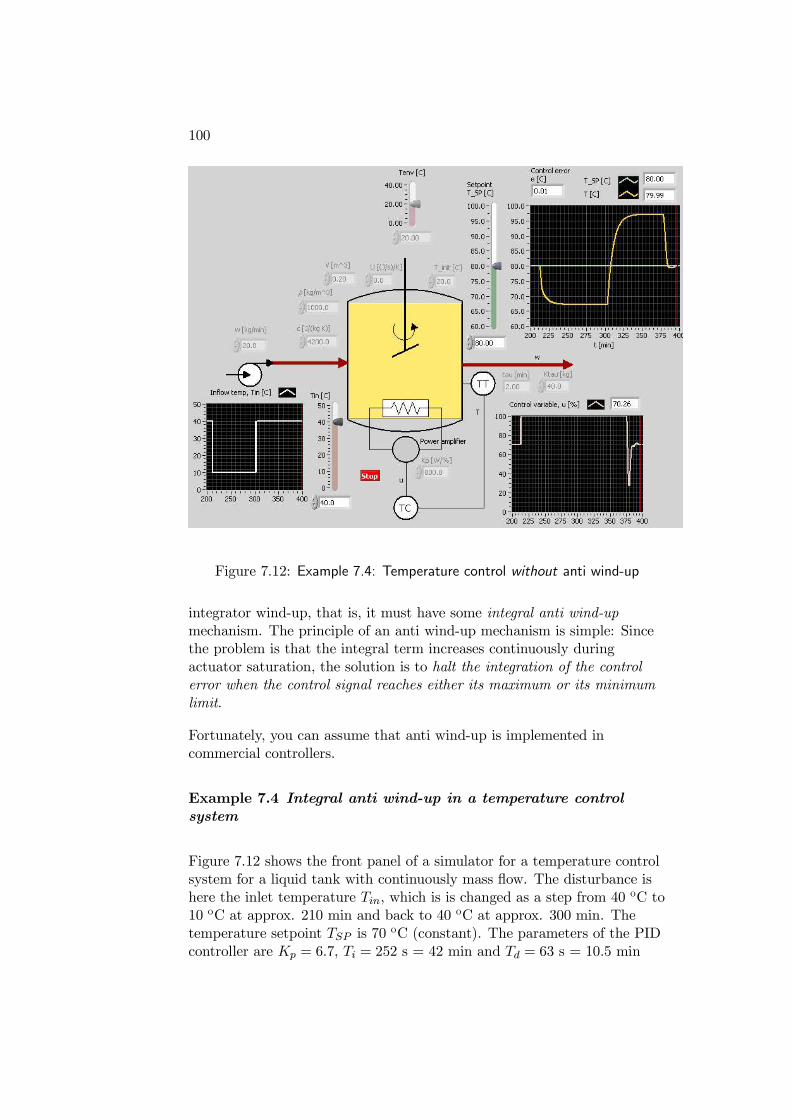
100

Figure 7.12: Example 7.4: Temperature control without anti wind-up

integrator wind-up, that is, it must have some integral anti wind-upmechanism. The principle of an anti wind-up mechanism is simple: Sincethe problem is that the integral term increases continuously duringactuator saturation, the solution is to halt the integration of the controlerror when the control signal reaches either its maximum or its minimumlimit.

Fortunately, you can assume that anti wind-up is implemented incommercial controllers.

Example 7.4 Integral anti wind-up in a temperature controlsystem

Figure 7.12 shows the front panel of a simulator for a temperature controlsystem for a liquid tank with continuously mass flow. The disturbance ishere the inlet temperature Tin, which is is changed as a step from 40 oC to10 oC at approx. 210 min and back to 40 oC at approx. 300 min. Thetemperature setpoint TSP is 70 oC (constant). The parameters of the PIDcontroller are Kp = 6.7, Ti = 252 s = 42 min and Td = 63 s = 10.5 min

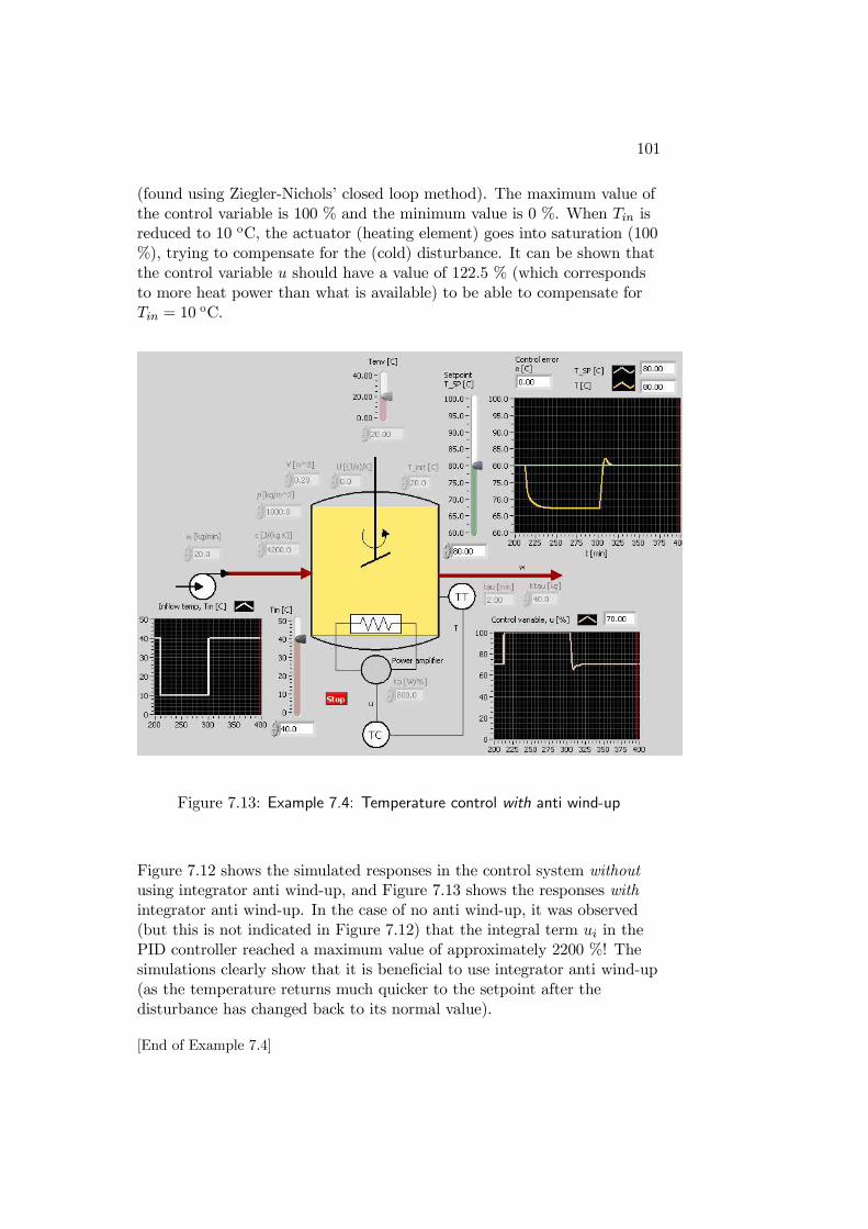
101

(found using Ziegler-Nichols’ closed loop method). The maximum value ofthe control variable is 100 % and the minimum value is 0 %. When Tin isreduced to 10 oC, the actuator (heating element) goes into saturation (100%), trying to compensate for the (cold) disturbance. It can be shown thatthe control variable u should have a value of 122.5 % (which correspondsto more heat power than what is available) to be able to compensate forTin = 10

oC.

Figure 7.13: Example 7.4: Temperature control with anti wind-up

Figure 7.12 shows the simulated responses in the control system withoutusing integrator anti wind-up, and Figure 7.13 shows the responses withintegrator anti wind-up. In the case of no anti wind-up, it was observed(but this is not indicated in Figure 7.12) that the integral term ui in thePID controller reached a maximum value of approximately 2200 %! Thesimulations clearly show that it is beneficial to use integrator anti wind-up(as the temperature returns much quicker to the setpoint after thedisturbance has changed back to its normal value).


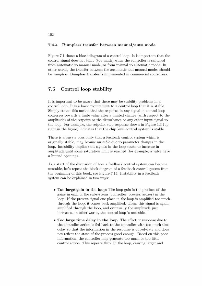
102

7.4.4 Bumpless transfer between manual/auto mode

Figure 7.1 shows a block diagram of a control loop. It is important that thecontrol signal does not jump (too much) when the controller is switchedfrom automatic to manual mode, or from manual to automatic mode. Inother words, the transfer between the automatic and manual modes shouldbe bumpless. Bumpless transfer is implemented in commercial controllers.

7.5 Control loop stability

It is important to be aware that there may be stability problems in acontrol loop. It is a basic requirement to a control loop that it is stable.Simply stated this means that the response in any signal in control loopconverges towards a finite value after a limited change (with respect to theamplitude) of the setpoint or the disturbance or any other input signal tothe loop. For example, the setpoint step response shown in Figure 1.3 (up,right in the figure) indicates that the chip level control system is stable.

There is always a possibility that a feedback control system which isoriginally stable, may become unstable due to parameter changes in theloop. Instability implies that signals in the loop starts to increase inamplitude until some saturation limit is reached (for example, a valve havea limited opening).

As a start of the discussion of how a feedback control system can becomeunstable, let’s repeat the block diagram of a feedback control system fromthe beginning of this book, see Figure 7.14. Instability in a feedbacksystem can be explained in two ways:

• Too large gain in the loop: The loop gain is the product of thegains in each of the subsystems (controller, process, sensor) in theloop. If the present signal one place in the loop is amplified too muchthrough the loop, it comes back amplified. Then, this signal is againamplified through the loop, and eventually the amplitude justincreases. In other words, the control loop is unstable.

• Too large time delay in the loop. The effect or response due tothe controller action is fed back to the controller with too much timedelay so that the information in the response is out-of-date and doesnot reflect the state of the process good enough. Based on this poorinformation, the controller may generate too much or too littlecontrol action. This repeats through the loop, causing larger and

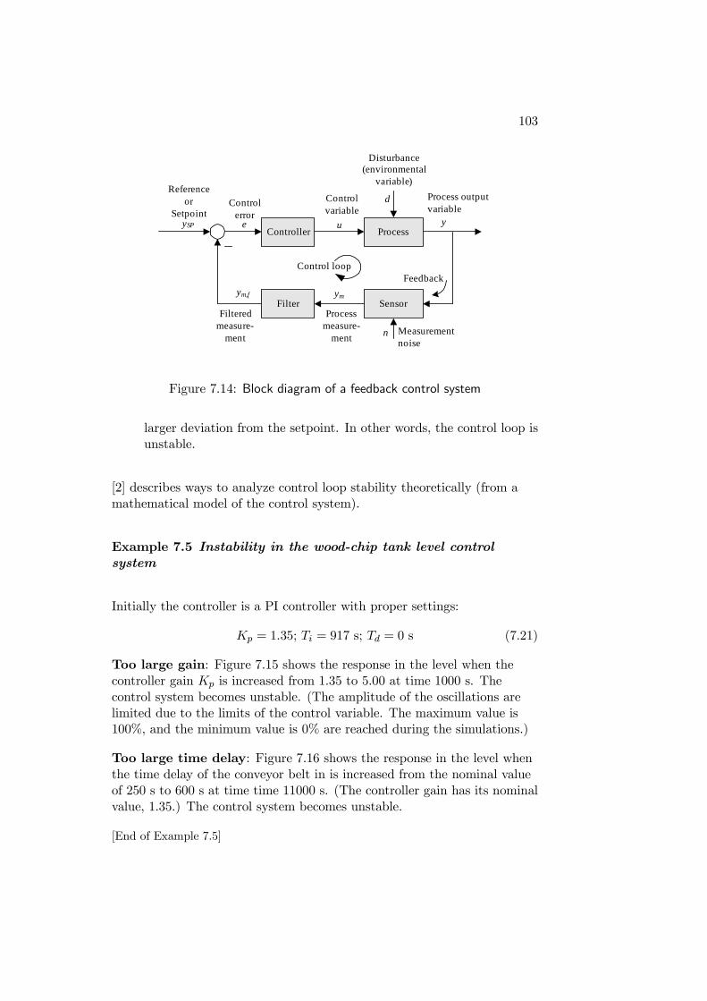
103

Process

Sensor

ySP ueController

y

dControlerror

Processmeasure-

ment

ym

n Measurement noise

Referenceor

Setpoint

Controlvariable


Feedback

Filterym,f

Filteredmeasure-

ment

Disturbance(environmental

variable)

Control loop

Figure 7.14: Block diagram of a feedback control system

larger deviation from the setpoint. In other words, the control loop isunstable.

[2] describes ways to analyze control loop stability theoretically (from amathematical model of the control system).

Example 7.5 Instability in the wood-chip tank level controlsystem

Initially the controller is a PI controller with proper settings:

Kp = 1.35; Ti = 917 s; Td = 0 s (7.21)

Too large gain: Figure 7.15 shows the response in the level when thecontroller gain Kp is increased from 1.35 to 5.00 at time 1000 s. Thecontrol system becomes unstable. (The amplitude of the oscillations arelimited due to the limits of the control variable. The maximum value is100%, and the minimum value is 0% are reached during the simulations.)

Too large time delay: Figure 7.16 shows the response in the level whenthe time delay of the conveyor belt in is increased from the nominal valueof 250 s to 600 s at time time 11000 s. (The controller gain has its nominalvalue, 1.35.) The control system becomes unstable.


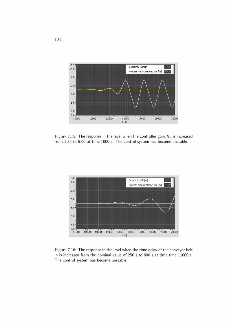
104

Figure 7.15: The response in the level when the controller gain Kp is increasedfrom 1.35 to 5.00 at time 1000 s. The control system has become unstable.

Figure 7.16: The response in the level when the time delay of the conveyor beltin is increased from the nominal value of 250 s to 600 s at time time 11000 s.The control system has become unstable.

Chapter 8

Feedforward control

8.1 Introduction

We know from Chapters 1.1 and 7 that feedback control — or error-drivencontrol — can bring the process output variable to or close to the setpoint.Feedback control is in most cases a sufficiently good control method. Butimprovements can be made, if required. A problem with feedback is thatthere is no adjustment of the control variable before the control error isdifferent from zero, since the control variable is adjusted as a function ofthe control error. This problem does not exist in feedforward control, whichmay be used as the only control method, or, more typically, as asupplement to feedback control.

In feedforward control there is a coupling from the setpoint and/or fromthe disturbance directly to the control variable, that is, a coupling from aninput signal to the control variable. The control variable adjustment is noterror-based. In stead it is based on knowledge about the process in theform of a mathematical model of the process and knowledge about ormeasurements of the process disturbances.

Perfect or ideal feedforward control gives zero control error for all types ofsignals (e.g. a sinusoid and a ramp) in the setpoint and in the disturbance.This sounds good, but feedforward control may be difficult to implementsince it assumes or is based on a mathematical process model and that allvariables of the model at any instant of time must have known valuesthrough measurements or in some other way. These requirements are nevercompletely satisfied, and therefore in practice the control error becomesdifferent from zero. We can however assume that the control error becomes

105

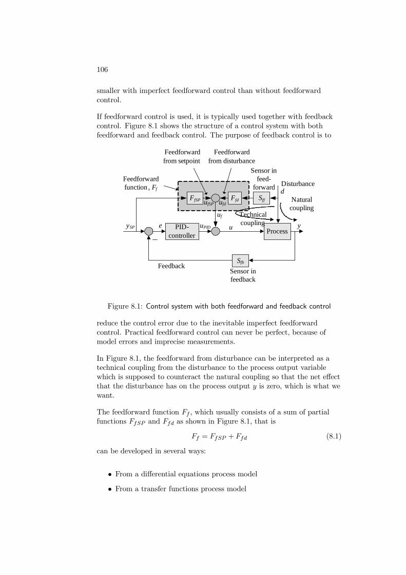
106

smaller with imperfect feedforward control than without feedforwardcontrol.

If feedforward control is used, it is typically used together with feedbackcontrol. Figure 8.1 shows the structure of a control system with bothfeedforward and feedback control. The purpose of feedback control is to

Process

d

yySP ue PID-controller

SffFfSP Ffd

Feedforwardfunction , Ff

Feedforward from setpoint

Feedforward from disturbance

uf

uPID

Feedback

ufdufSPNaturalcoupling

Technical coupling

Sfb

Sensor in feed-

forward

Sensor in feedback

Disturbance

Figure 8.1: Control system with both feedforward and feedback control

reduce the control error due to the inevitable imperfect feedforwardcontrol. Practical feedforward control can never be perfect, because ofmodel errors and imprecise measurements.

In Figure 8.1, the feedforward from disturbance can be interpreted as atechnical coupling from the disturbance to the process output variablewhich is supposed to counteract the natural coupling so that the net effectthat the disturbance has on the process output y is zero, which is what wewant.

The feedforward function Ff , which usually consists of a sum of partialfunctions FfSP and Ffd as shown in Figure 8.1, that is

Ff = FfSP + Ffd (8.1)

can be developed in several ways:

• From a differential equations process model

• From a transfer functions process model

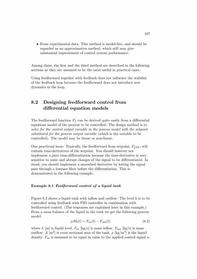
107

• From experimental data. This method is model-free, and should beregarded as an approximative method, which still may givesubstantial improvement of control system performance.

Among these, the first and the third method are described in the followingsections as they are assumed to be the most useful in practical cases.

Using feedforward together with feedback does not influence the stabilityof the feedback loop because the feedforward does not introduce newdynamics in the loop.

8.2 Designing feedforward control fromdifferential equation models

The feedforward function Ff can be derived quite easily from a differentialequations model of the process to be controlled. The design method is tosolve for the control output variable in the process model with the setpointsubstituted for the process output variable (which is the variable to becontrolled). The model may be linear or non-linear.

One practicual issue: Typically, the feedforward from setpoint, FfSP , willcontain time-derivatives of the setpoint. You should however notimplement a pure time-differentiation because the time-derivative is verysensitive to noise and abrupt changes of the signal to be differentiated. Instead, you should implement a smoothed derivative by letting the signalpass through a lowpass filter before the differentiation. This isdemonstrated in the following example.

Example 8.1 Feedforward control of a liquid tank

Figure 8.2 shows a liquid tank with inflow and outflow. The level h is to becontrolled using feedback with PID controller in combination withfeedforward control. (The responses are explained later in this example.)From a mass balance of the liquid in the tank we get the following processmodel:

ρAh(t) = Fin(t)− Fout(t) (8.2)

where h [m] is liquid level, Fin [kg/s] is mass inflow, Fout [kg/s] is massoutflow, A [m2] is cross sectional area of the tank, ρ [kg/m3] is the liquiddensity. Fin is assumed to be equal in value to the applied control signal u.

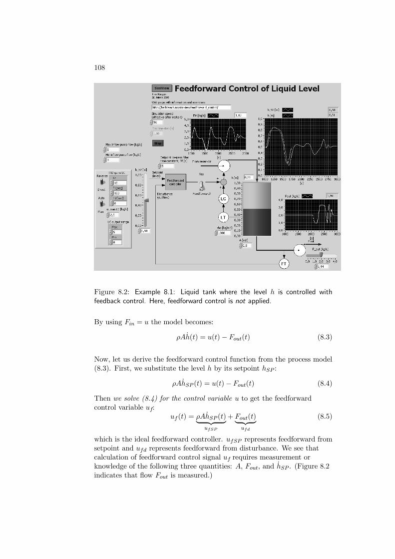
108

Figure 8.2: Example 8.1: Liquid tank where the level h is controlled withfeedback control. Here, feedforward control is not applied.

By using Fin = u the model becomes:

ρAh(t) = u(t)− Fout(t) (8.3)

Now, let us derive the feedforward control function from the process model(8.3). First, we substitute the level h by its setpoint hSP :

ρAhSP (t) = u(t)− Fout(t) (8.4)

Then we solve (8.4) for the control variable u to get the feedforwardcontrol variable uf:

uf (t) = ρAhSP (t) ufSP

+ Fout(t) ufd

(8.5)

which is the ideal feedforward controller. ufSP represents feedforward fromsetpoint and ufd represents feedforward from disturbance. We see thatcalculation of feedforward control signal uf requires measurement orknowledge of the following three quantities: A, Fout, and hSP . (Figure 8.2indicates that flow Fout is measured.)

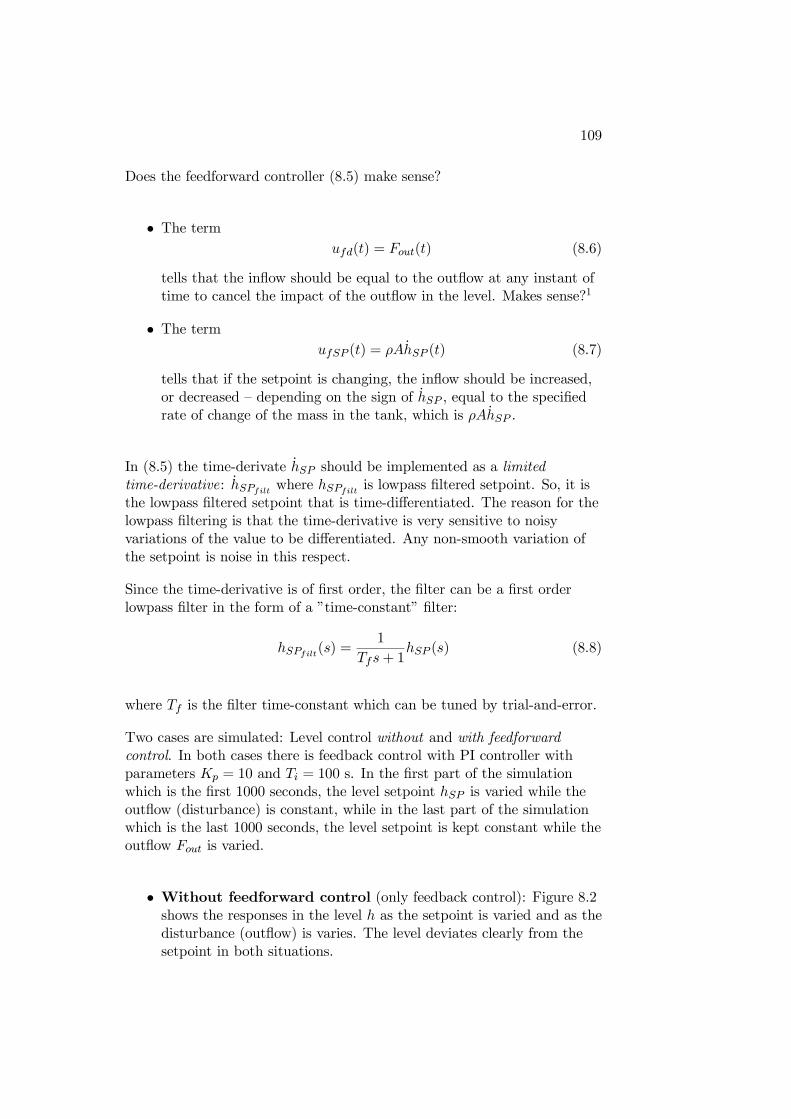
109

Does the feedforward controller (8.5) make sense?

• The termufd(t) = Fout(t) (8.6)

tells that the inflow should be equal to the outflow at any instant oftime to cancel the impact of the outflow in the level. Makes sense?1

• The termufSP (t) = ρAhSP (t) (8.7)

tells that if the setpoint is changing, the inflow should be increased,or decreased — depending on the sign of hSP , equal to the specifiedrate of change of the mass in the tank, which is ρAhSP .

In (8.5) the time-derivate hSP should be implemented as a limitedtime-derivative: hSPfilt where hSPfilt is lowpass filtered setpoint. So, it isthe lowpass filtered setpoint that is time-differentiated. The reason for thelowpass filtering is that the time-derivative is very sensitive to noisyvariations of the value to be differentiated. Any non-smooth variation ofthe setpoint is noise in this respect.

Since the time-derivative is of first order, the filter can be a first orderlowpass filter in the form of a ”time-constant” filter:

hSPfilt(s) =1

Tfs+ 1hSP (s) (8.8)

where Tf is the filter time-constant which can be tuned by trial-and-error.

Two cases are simulated: Level control without and with feedforwardcontrol. In both cases there is feedback control with PI controller withparameters Kp = 10 and Ti = 100 s. In the first part of the simulationwhich is the first 1000 seconds, the level setpoint hSP is varied while theoutflow (disturbance) is constant, while in the last part of the simulationwhich is the last 1000 seconds, the level setpoint is kept constant while theoutflow Fout is varied.

• Without feedforward control (only feedback control): Figure 8.2shows the responses in the level h as the setpoint is varied and as thedisturbance (outflow) is varies. The level deviates clearly from thesetpoint in both situations.

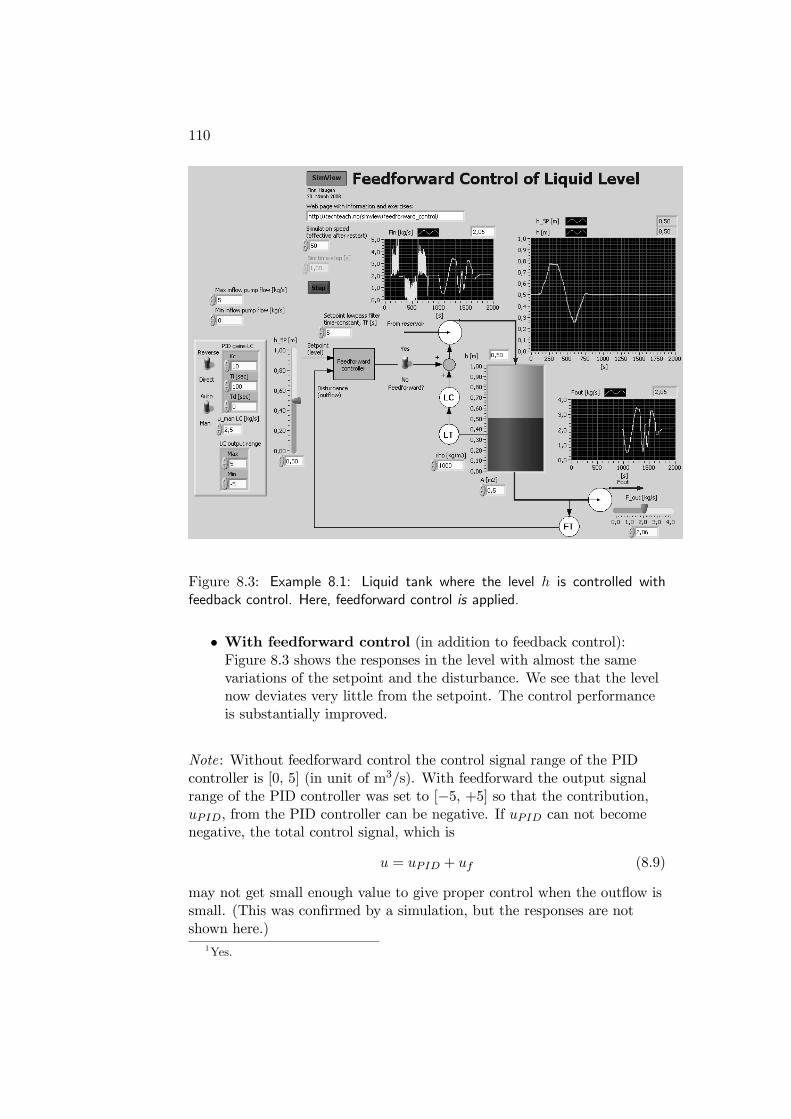
110

Figure 8.3: Example 8.1: Liquid tank where the level h is controlled withfeedback control. Here, feedforward control is applied.

• With feedforward control (in addition to feedback control):Figure 8.3 shows the responses in the level with almost the samevariations of the setpoint and the disturbance. We see that the levelnow deviates very little from the setpoint. The control performanceis substantially improved.

Note: Without feedforward control the control signal range of the PIDcontroller is [0, 5] (in unit of m3/s). With feedforward the output signalrange of the PID controller was set to [−5, +5] so that the contribution,uPID, from the PID controller can be negative. If uPID can not becomenegative, the total control signal, which is

u = uPID + uf (8.9)

may not get small enough value to give proper control when the outflow issmall. (This was confirmed by a simulation, but the responses are notshown here.)

1Yes.

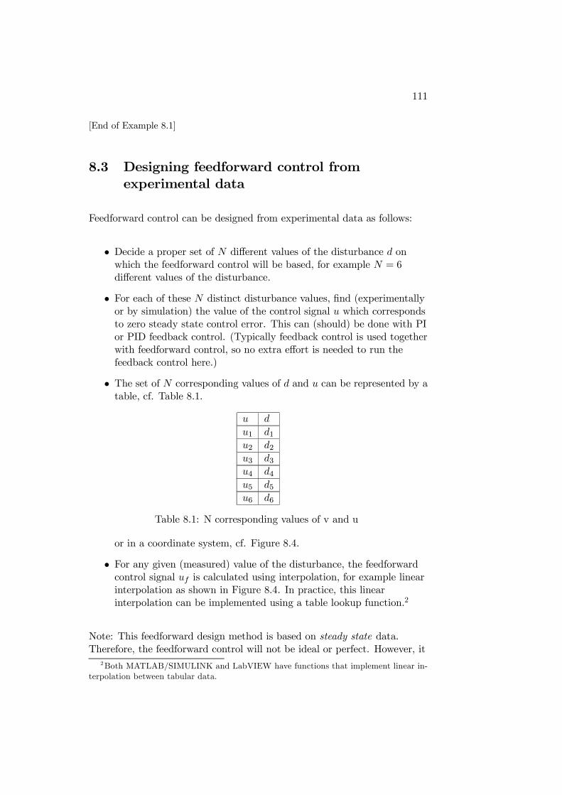
111


8.3 Designing feedforward control fromexperimental data

Feedforward control can be designed from experimental data as follows:

• Decide a proper set of N different values of the disturbance d onwhich the feedforward control will be based, for example N = 6different values of the disturbance.

• For each of these N distinct disturbance values, find (experimentallyor by simulation) the value of the control signal u which correspondsto zero steady state control error. This can (should) be done with PIor PID feedback control. (Typically feedback control is used togetherwith feedforward control, so no extra effort is needed to run thefeedback control here.)

• The set of N corresponding values of d and u can be represented by atable, cf. Table 8.1.

u d

u1 d1u2 d2u3 d3u4 d4u5 d5u6 d6

Table 8.1: N corresponding values of v and u

or in a coordinate system, cf. Figure 8.4.

• For any given (measured) value of the disturbance, the feedforwardcontrol signal uf is calculated using interpolation, for example linearinterpolation as shown in Figure 8.4. In practice, this linearinterpolation can be implemented using a table lookup function.2

Note: This feedforward design method is based on steady state data.Therefore, the feedforward control will not be ideal or perfect. However, it

2Both MATLAB/SIMULINK and LabVIEW have functions that implement linear in-terpolation between tabular data.

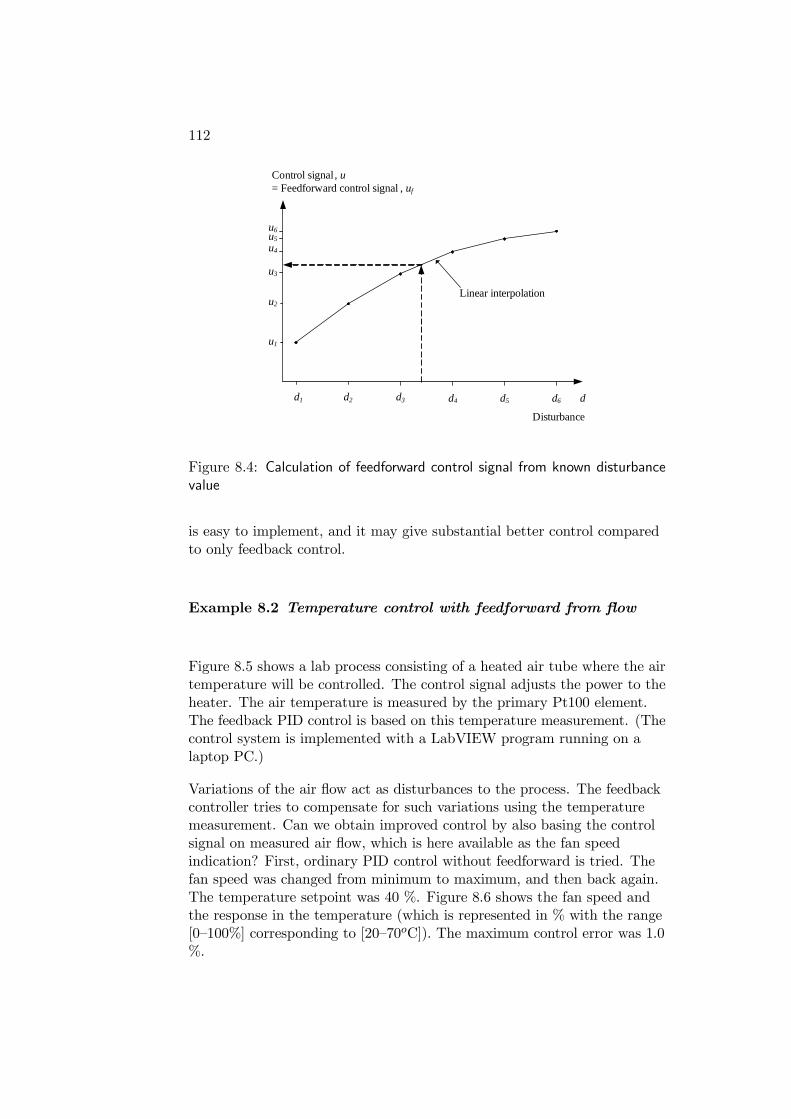
112

d1 d2 d3 d

u3

Linear interpolationu2

u1

d4 d5 d6

u4

u5

u6

Disturbance

Control signal, u= Feedforward control signal , uf

Figure 8.4: Calculation of feedforward control signal from known disturbancevalue

is easy to implement, and it may give substantial better control comparedto only feedback control.

Example 8.2 Temperature control with feedforward from flow

Figure 8.5 shows a lab process consisting of a heated air tube where the airtemperature will be controlled. The control signal adjusts the power to theheater. The air temperature is measured by the primary Pt100 element.The feedback PID control is based on this temperature measurement. (Thecontrol system is implemented with a LabVIEW program running on alaptop PC.)

Variations of the air flow act as disturbances to the process. The feedbackcontroller tries to compensate for such variations using the temperaturemeasurement. Can we obtain improved control by also basing the controlsignal on measured air flow, which is here available as the fan speedindication? First, ordinary PID control without feedforward is tried. Thefan speed was changed from minimum to maximum, and then back again.The temperature setpoint was 40 %. Figure 8.6 shows the fan speed andthe response in the temperature (which is represented in % with the range[0—100%] corresponding to [20—70oC]). The maximum control error was 1.0%.

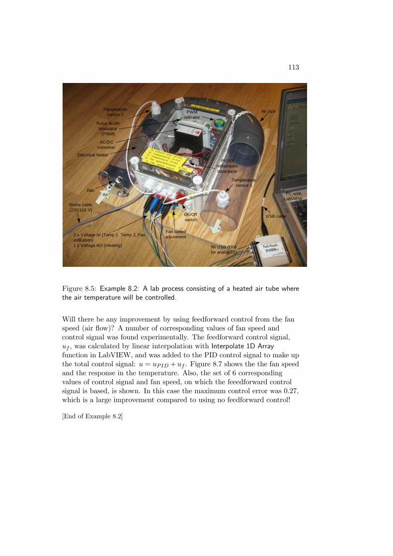
113

Temperature sensor 1

Temperature sensor 2

NI USB-6008for analog I /O

Fan speed adjustment

On/Offswitch

PC with LabVIEW

USB cable

Electrical heater

Fan

Mains cable(220/110 V)

3 x Voltage AI (Temp 1, Temp 2, Fan indication)1 x Voltage AO (Heating)

Air

Pulse Width Modulator

(PWM)

PWMindicator

AC/DC converter

Pt100/milliamperetransducer

Air pipe

Figure 8.5: Example 8.2: A lab process consisting of a heated air tube wherethe air temperature will be controlled.

Will there be any improvement by using feedforward control from the fanspeed (air flow)? A number of corresponding values of fan speed andcontrol signal was found experimentally. The feedforward control signal,uf , was calculated by linear interpolation with Interpolate 1D Arrayfunction in LabVIEW, and was added to the PID control signal to make upthe total control signal: u = uPID + uf . Figure 8.7 shows the the fan speedand the response in the temperature. Also, the set of 6 correspondingvalues of control signal and fan speed, on which the feeedforward controlsignal is based, is shown. In this case the maximum control error was 0.27,which is a large improvement compared to using no feedforward control!


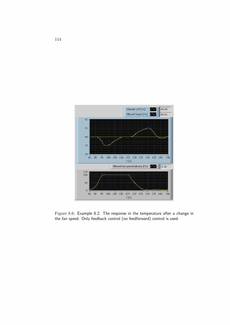
114

Figure 8.6: Example 8.2: The response in the temperature after a change inthe fan speed. Only feedback control (no feedforward) control is used.

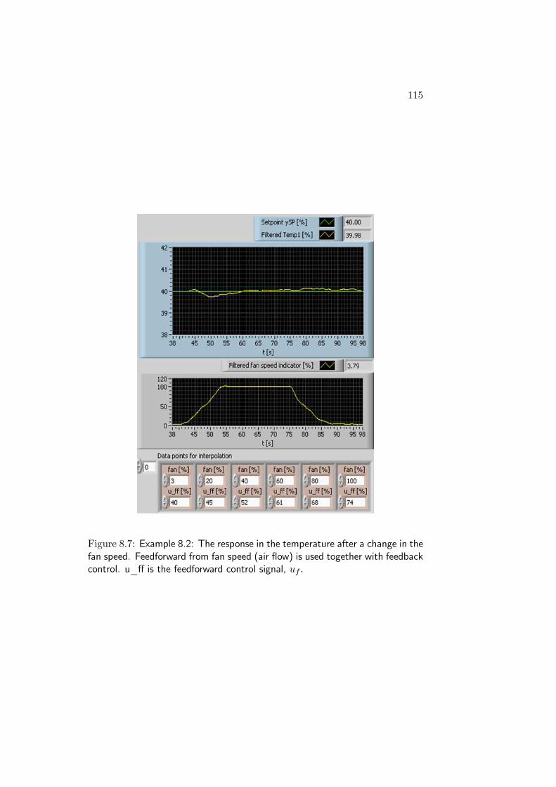
115

Figure 8.7: Example 8.2: The response in the temperature after a change in thefan speed. Feedforward from fan speed (air flow) is used together with feedbackcontrol. u_ff is the feedforward control signal, uf .

Chapter 9

Controller equipment

This chapter gives an overview over various kinds of commercial controllerequipment.

9.1 Process controllers

A process controller is a single controller unit which can be used to controlone process output variable. Figure 9.1 shows an example of a processcontroller (ABB’s ECA600). Figure 9.2 shows the backplane of theECA600 controller. Both analog and digital sensors (inputs, AI and DI)and actuators (outputs, AO and DO) can be connected to terminals at thebackplane, which also has connectors for digital communication (Modbuswith RS485 and serial with RS232) with computers or other devices.

Today new process controllers are implemented digitally with amicroprocessor. The PID controller function is in the form of a programwhich runs cyclically, e.g. each 0.1s, which then is called the time step ofthe controller. Earlier, controllers were build using analog electronics, andeven earlier, pneumatic and mechanical components were used. Suchcontrollers are still in use today in some factories since they work well andare safe in dangerous (explosive) areas.

Here is a list of typical characteristics of process controllers:

• The front panel of the controller has vertical bar indicators and/ornumeric displays showing, see Figure 9.1,

— the process measurement signal (a common symbol is PV —

117

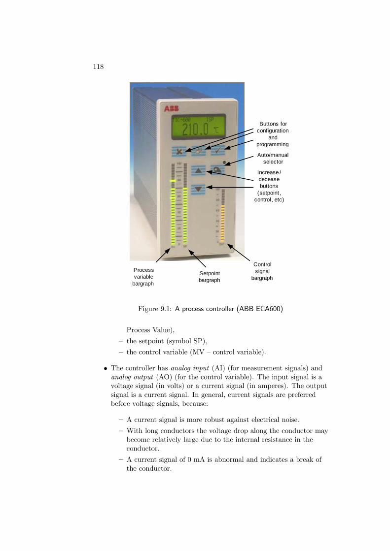
118

Setpoint bargraph

Process variable

bargraph

Controlsignal

bargraph

Increase /deceasebuttons

(setpoint , control, etc)

Buttons for configuration

and programming

Auto/manualselector

Figure 9.1: A process controller (ABB ECA600)

Process Value),

— the setpoint (symbol SP),

— the control variable (MV — control variable).

• The controller has analog input (AI) (for measurement signals) andanalog output (AO) (for the control variable). The input signal is avoltage signal (in volts) or a current signal (in amperes). The outputsignal is a current signal. In general, current signals are preferredbefore voltage signals, because:

— A current signal is more robust against electrical noise.

— With long conductors the voltage drop along the conductor maybecome relatively large due to the internal resistance in theconductor.

— A current signal of 0 mA is abnormal and indicates a break ofthe conductor.

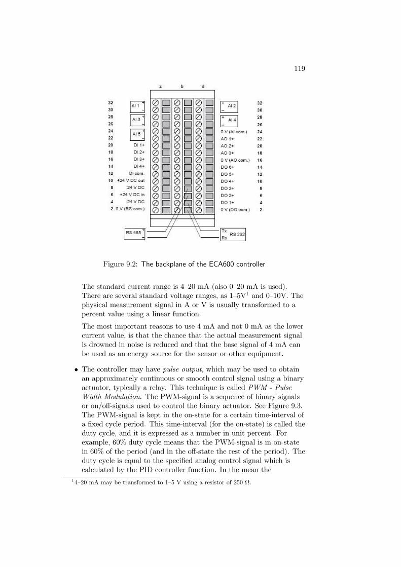
119

Figure 9.2: The backplane of the ECA600 controller

The standard current range is 4—20 mA (also 0—20 mA is used).There are several standard voltage ranges, as 1—5V1 and 0—10V. Thephysical measurement signal in A or V is usually transformed to apercent value using a linear function.

The most important reasons to use 4 mA and not 0 mA as the lowercurrent value, is that the chance that the actual measurement signalis drowned in noise is reduced and that the base signal of 4 mA canbe used as an energy source for the sensor or other equipment.

• The controller may have pulse output, which may be used to obtainan approximately continuous or smooth control signal using a binaryactuator, typically a relay. This technique is called PWM - PulseWidth Modulation. The PWM-signal is a sequence of binary signalsor on/off-signals used to control the binary actuator. See Figure 9.3.The PWM-signal is kept in the on-state for a certain time-interval ofa fixed cycle period. This time-interval (for the on-state) is called theduty cycle, and it is expressed as a number in unit percent. Forexample, 60% duty cycle means that the PWM-signal is in on-statein 60% of the period (and in the off-state the rest of the period). Theduty cycle is equal to the specified analog control signal which iscalculated by the PID controller function. In the mean the

14—20 mA may be transformed to 1—5 V using a resistor of 250 Ω.

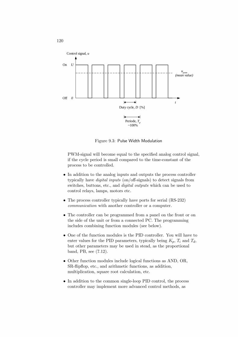
120

t

upwm(mean value)

Duty cycle, D [%]

Periode, Tp~100%

U

0

On

Off

Control signal, u

Figure 9.3: Pulse Width Modulation

PWM-signal will become equal to the specified analog control signal,if the cycle period is small compared to the time-constant of theprocess to be controlled.

• In addition to the analog inputs and outputs the process controllertypically have digital inputs (on/off-signals) to detect signals fromswitches, buttons, etc., and digital outputs which can be used tocontrol relays, lamps, motors etc.

• The process controller typically have ports for serial (RS-232)communication with another controller or a computer.

• The controller can be programmed from a panel on the front or onthe side of the unit or from a connected PC. The programmingincludes combining function modules (see below).

• One of the function modules is the PID controller. You will have toenter values for the PID parameters, typically being Kp, Ti and Td,but other parameters may be used in stead, as the proportionalband, PB, see (7.12).

• Other function modules include logical functions as AND, OR,SR-flipflop, etc., and arithmetic functions, as addition,multiplication, square root calculation, etc.

• In addition to the common single-loop PID control, the processcontroller may implement more advanced control methods, as

121

feedforward control (cf. Chapter 8) gain scheduling PID control(10.5.3), cascade control (11.1) and ratio control (11.2).

• The operator can adjust the setpoint internally (locally) on thecontroller, but it is usually possible to use an external setpoint, too,which may come from another controller (as in cascade control) orfrom a sensor (as in ratio control) or from a computer whichcalculates the setpoint as a result of a plantwide control strategy.

• The operator can take over the control by switching the processcontroller from automatic mode to manual mode. This may benecessary if the control program is to be modified, and at first-timestart-up. In manual mode the operator adjusts the controller output(which is used as the manipulating variable of the process) manuallyor directly, while in automatic mode the control output is calculatedaccording to the control function (typically PID control function).

• Many controllers have the possibility of auto-tuning, which meansthat the process controller — initialized by the operator — calculatesproper values of the controller parameters based on someautomatically conducted experiment on the process to be controlled.An even more advanced option which may be implemented is anadaptive PID controller where the PID parameters are calculatedcontinuously from an estimated process model.

• The operator can define alarm limits of the measurement signal. Thealarm can be indicated on the front panel of the controller unit, andthe alarm limits can be used by the control program to set the valueof a digital output of the process controller to turn on e.g. an alarmlamp.

Figure 9.4 shows a section of the data sheet of the controller ECA600shown in Figure 9.1.

9.2 Programmable logical controller (PLC)

PLC s are common in industrial automation. Figure 9.5 shows a PLCsystem (Mitsubishi FX2N). PLC is short for Programmable LogicalController. PLC-systems are modular systems for logical (binary) andsequential control of valves, motors, lamps etc. Modern PLCs includesfunction modules for PID control. The programming is usually executedon a PC, and the PLC-program is then downloaded (transfered) to theCPU in the PLC-system which then can be disconnected from the PC. The

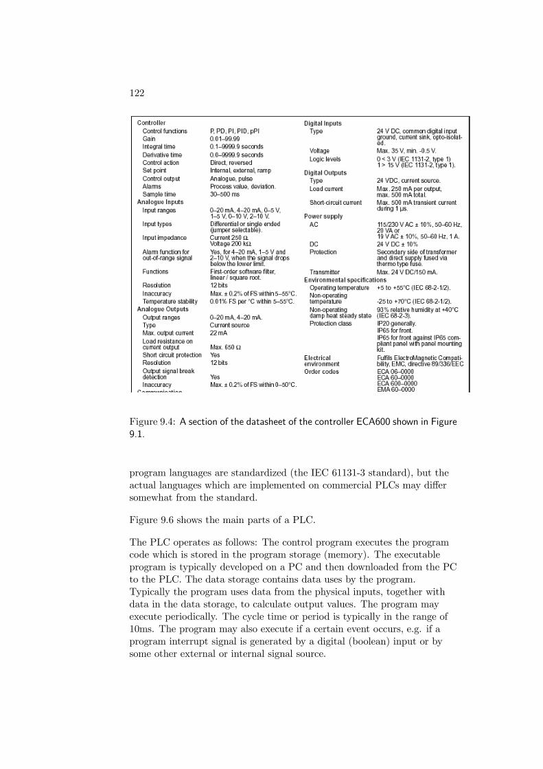
122

Figure 9.4: A section of the datasheet of the controller ECA600 shown in Figure9.1.

program languages are standardized (the IEC 61131-3 standard), but theactual languages which are implemented on commercial PLCs may differsomewhat from the standard.

Figure 9.6 shows the main parts of a PLC.

The PLC operates as follows: The control program executes the programcode which is stored in the program storage (memory). The executableprogram is typically developed on a PC and then downloaded from the PCto the PLC. The data storage contains data uses by the program.Typically the program uses data from the physical inputs, together withdata in the data storage, to calculate output values. The program mayexecute periodically. The cycle time or period is typically in the range of10ms. The program may also execute if a certain event occurs, e.g. if aprogram interrupt signal is generated by a digital (boolean) input or bysome other external or internal signal source.

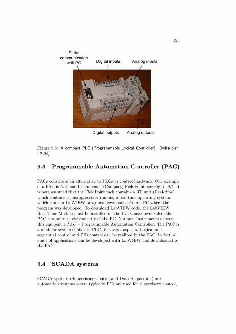
123

Digital outputs

Digital inputs

Serial communication

with PC Analog inputs

Analog outputs

Figure 9.5: A compact PLC (Programmable Locical Controller). (MitsubishiFX2N)

9.3 Programmable Automation Controller (PAC)

PACs constitute an alternative to PLCs as control hardware. One exampleof a PAC is National Instruments’ (Compact) FieldPoint, see Figure 9.7. Itis here assumed that the FieldPoint rack contains a RT unit (Real-time)which contains a microprocessor running a real-time operating systemwhich can run LabVIEW programs downloaded from a PC where theprogram was developed. To download LabVIEW code, the LabVIEWReal-Time Module must be installed on the PC. Once downloaded, thePAC can be run independently of the PC. National Instruments denotesthis equipent a PAC — Programmable Automation Controller. The PAC isa modular system similar to PLCs in several aspects. Logical andsequential control and PID control can be realized in the PAC. In fact, allkinds of applications can be developed with LabVIEW and downloaded tothe PAC.

9.4 SCADA systems

SCADA systems (Supervisory Control and Data Acquisition) areautomation systems where typically PCs are used for supervisory control,

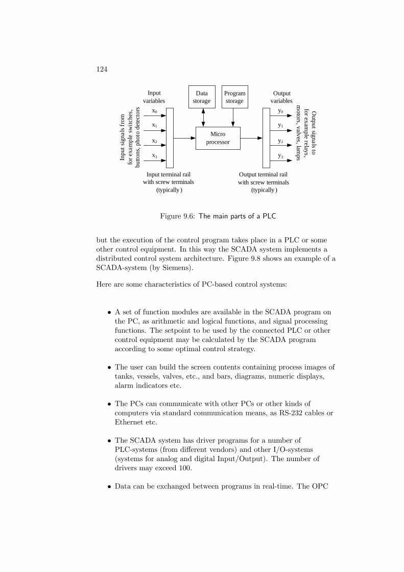
124

Microprocessor

Data storage

Program storage

x0

x1

Inputvariables

Input terminal railwith screw terminals

(typically )

x2

x3Inp

ut

sig

nals

fro

mfo

r ex

am

ple

sw

itch

es,

butto

ns,

ph

oto

dete

cto

rs

y0

y1

Outputvariables

y2

y3

Ou

tpu

t sign

als to

for exam

ple relays

,m

oto

rs, valves

, lamps

Output terminal railwith screw terminals

(typically )

Figure 9.6: The main parts of a PLC

but the execution of the control program takes place in a PLC or someother control equipment. In this way the SCADA system implements adistributed control system architecture. Figure 9.8 shows an example of aSCADA-system (by Siemens).

Here are some characteristics of PC-based control systems:

• A set of function modules are available in the SCADA program onthe PC, as arithmetic and logical functions, and signal processingfunctions. The setpoint to be used by the connected PLC or othercontrol equipment may be calculated by the SCADA programaccording to some optimal control strategy.

• The user can build the screen contents containing process images oftanks, vessels, valves, etc., and bars, diagrams, numeric displays,alarm indicators etc.

• The PCs can communicate with other PCs or other kinds ofcomputers via standard communication means, as RS-232 cables orEthernet etc.

• The SCADA system has driver programs for a number ofPLC-systems (from different vendors) and other I/O-systems(systems for analog and digital Input/Output). The number ofdrivers may exceed 100.

• Data can be exchanged between programs in real-time. The OPC

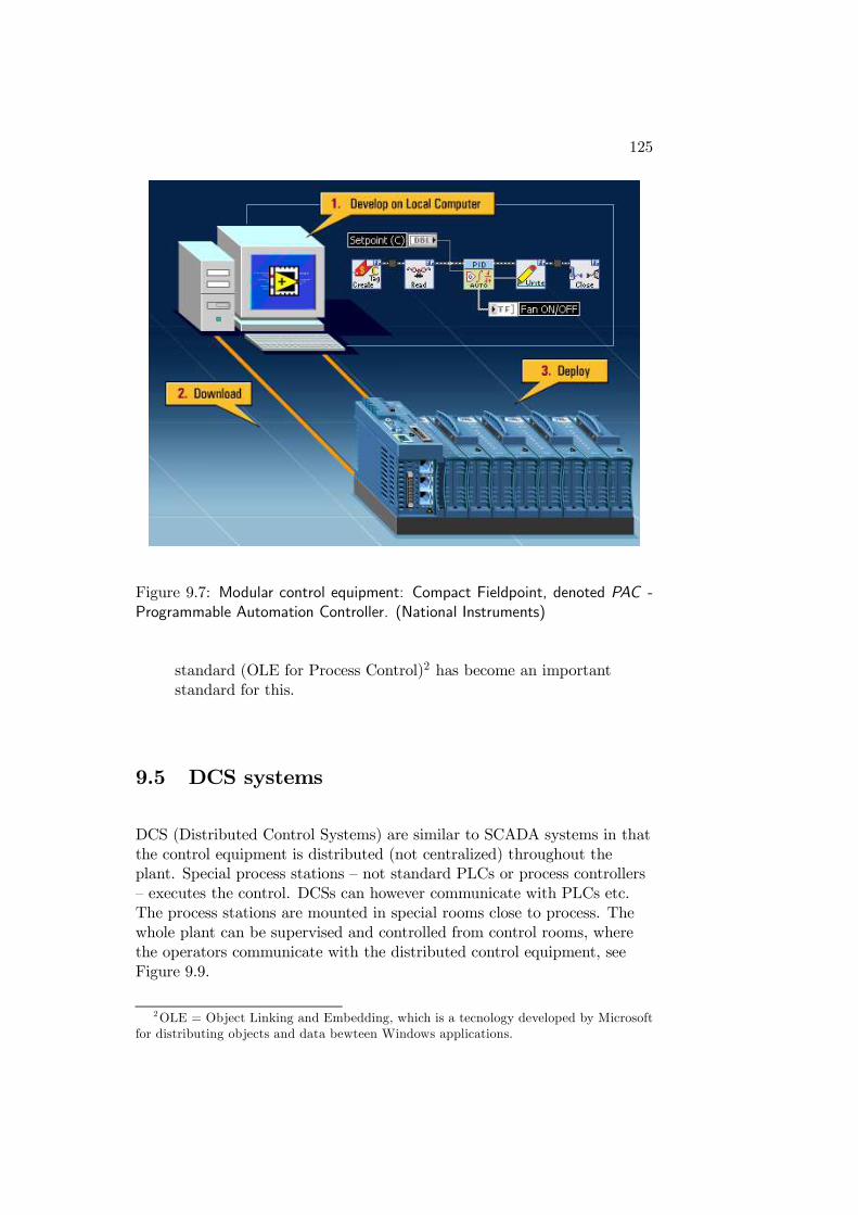
125

Figure 9.7: Modular control equipment: Compact Fieldpoint, denoted PAC -Programmable Automation Controller. (National Instruments)

standard (OLE for Process Control)2 has become an importantstandard for this.

9.5 DCS systems

DCS (Distributed Control Systems) are similar to SCADA systems in thatthe control equipment is distributed (not centralized) throughout theplant. Special process stations — not standard PLCs or process controllers— executes the control. DCSs can however communicate with PLCs etc.The process stations are mounted in special rooms close to process. Thewhole plant can be supervised and controlled from control rooms, wherethe operators communicate with the distributed control equipment, seeFigure 9.9.

2OLE = Object Linking and Embedding, which is a tecnology developed by Microsoftfor distributing objects and data bewteen Windows applications.

126

9.6 Embedded controllers in motors etc.

Producers of electrical and hydraulic servo motors also offers controllers forthe motors. These controllers are usually embedded in the motor drivesystem, as a separate physical unit connected to the motor via cables. Thecontrollers implement speed control and/or positional control. Figure 9.10shows an example of a servo amplifier for DC-motor. The servo amplifierhave an embedded PI controller which the user can tune via screws on theservo amplifier card.

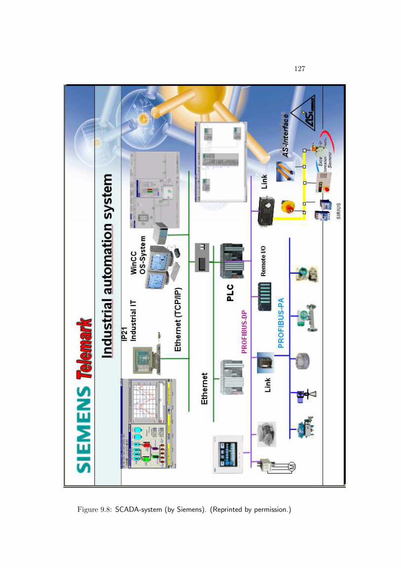
127

Figure 9.8: SCADA-system (by Siemens). (Reprinted by permission.)

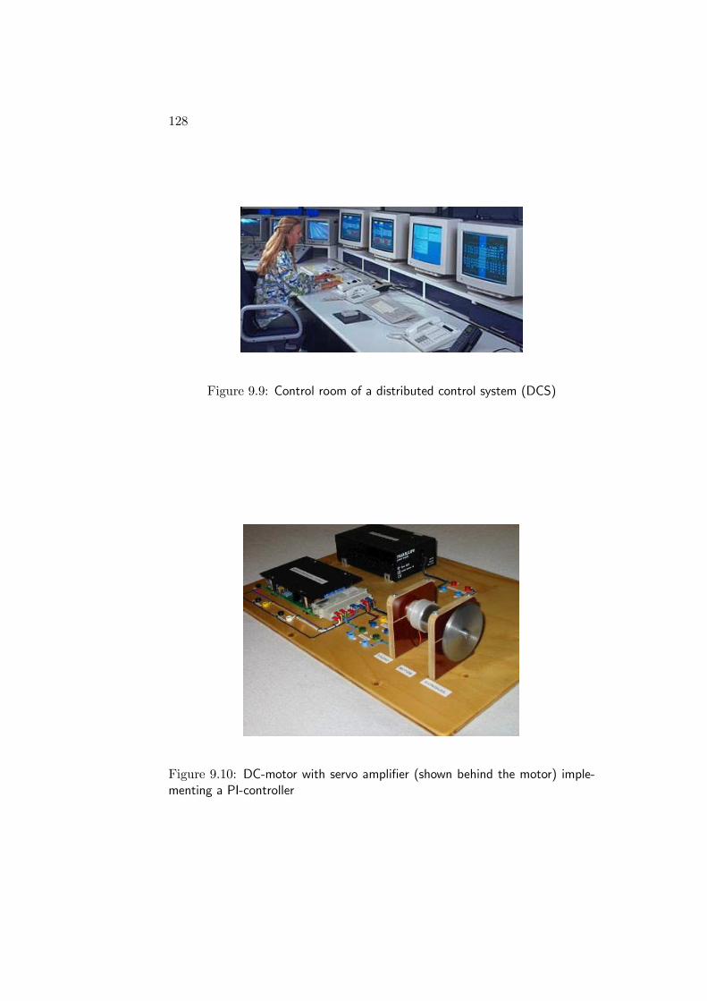
128

Figure 9.9: Control room of a distributed control system (DCS)

Figure 9.10: DC-motor with servo amplifier (shown behind the motor) imple-menting a PI-controller

Chapter 10

Tuning of PID controllers

10.1 Introduction

This chapter describes two methods for calculating proper values of thePID parameters Kp, Ti and Td, i.e. controller tuning. These two methodsare:

• The Good Gain method [3] which is a simple experimentalmethod which can be used without any knowledge about the processto be controlled. (Of course, if you have a process model, you can usethe Good Gain method on a simulator in stead of on the physicalprocess.)

• Skogestad’s method [7] which is a model-based method. It isassumed that you have mathematical model of the process (a transferfunction model). It does not matter how you have derived thetransfer function — it can stem from a model derived from physicalprinciples (as described in Ch. 3), or from calculation of modelparameters (e.g. gain, time-constant and time-delay) from anexperimental response, typically a step response experiment with theprocess (step on the process input).

A large number of tuning methods exists [1], but it is my view that theabove methods will cover most practical cases. What about the famousZiegler-Nichols’ methods — the Ultimate Gain method (or Closed-Loopmethod) and the Process Reaction curve method (the Open-Loopmethod)?[8] The Good Gain method has actually many similarities withthe Ultimate Gain method, but the latter method has one serious

129

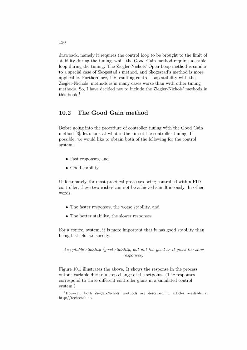
130

drawback, namely it requires the control loop to be brought to the limit ofstability during the tuning, while the Good Gain method requires a stableloop during the tuning. The Ziegler-Nichols’ Open-Loop method is similarto a special case of Skogestad’s method, and Skogestad’s method is moreapplicable. Furthermore, the resulting control loop stability with theZiegler-Nichols’ methods is in many cases worse than with other tuningmethods. So, I have decided not to include the Ziegler-Nichols’ methods inthis book.1

10.2 The Good Gain method

Before going into the procedure of controller tuning with the Good Gainmethod [3], let’s look at what is the aim of the controller tuning. Ifpossible, we would like to obtain both of the following for the controlsystem:

• Fast responses, and

• Good stability

Unfortunately, for most practical processes being controlled with a PIDcontroller, these two wishes can not be achieved simultaneously. In otherwords:

• The faster responses, the worse stability, and

• The better stability, the slower responses.

For a control system, it is more important that it has good stability thanbeing fast. So, we specify:

Acceptable stability (good stability, but not too good as it gives too slowresponses)

Figure 10.1 illustrates the above. It shows the response in the processoutput variable due to a step change of the setpoint. (The responsescorrespond to three different controller gains in a simulated controlsystem.)

1However, both Ziegler-Nichols’ methods are described in articles available athttp://techteach.no.

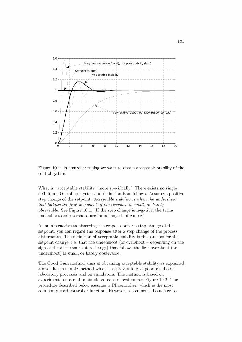
131

0 2 4 6 8 10 12 14 16 18 200

0.2

0.4

0.6

0.8

1

1.2

1.4

1.6

Very stable (good), but slow response (bad)

Very fast response (good), but poor stability (bad)

Setpoint (a step)Acceptable stability

Figure 10.1: In controller tuning we want to obtain acceptable stability of thecontrol system.

What is “acceptable stability” more specifically? There exists no singledefinition. One simple yet useful definition is as follows. Assume a positivestep change of the setpoint. Acceptable stability is when the undershootthat follows the first overshoot of the response is small, or barelyobservable. See Figure 10.1. (If the step change is negative, the termsundershoot and overshoot are interchanged, of course.)

As an alternative to observing the response after a step change of thesetpoint, you can regard the response after a step change of the processdisturbance. The definition of acceptable stability is the same as for thesetpoint change, i.e. that the undershoot (or overshoot — depending on thesign of the disturbance step change) that follows the first overshoot (orundershoot) is small, or barely observable.

The Good Gain method aims at obtaining acceptable stability as explainedabove. It is a simple method which has proven to give good results onlaboratory processes and on simulators. The method is based onexperiments on a real or simulated control system, see Figure 10.2. Theprocedure described below assumes a PI controller, which is the mostcommonly used controller function. However, a comment about how to

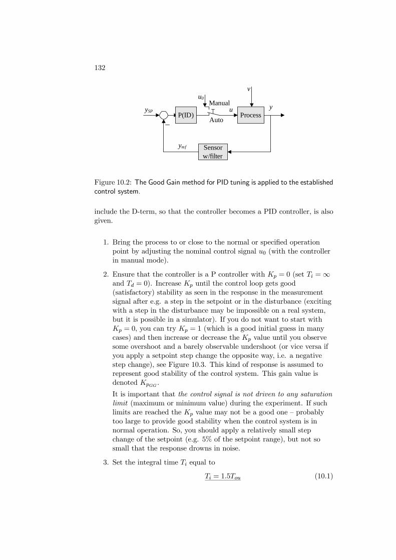
132

Process

Sensorw/filter

v

y

ymf

ySP uP(ID)

u0

Auto

Manual

Figure 10.2: The Good Gain method for PID tuning is applied to the establishedcontrol system.

include the D-term, so that the controller becomes a PID controller, is alsogiven.

1. Bring the process to or close to the normal or specified operationpoint by adjusting the nominal control signal u0 (with the controllerin manual mode).

2. Ensure that the controller is a P controller with Kp = 0 (set Ti =∞and Td = 0). Increase Kp until the control loop gets good(satisfactory) stability as seen in the response in the measurementsignal after e.g. a step in the setpoint or in the disturbance (excitingwith a step in the disturbance may be impossible on a real system,but it is possible in a simulator). If you do not want to start withKp = 0, you can try Kp = 1 (which is a good initial guess in manycases) and then increase or decrease the Kp value until you observesome overshoot and a barely observable undershoot (or vice versa ifyou apply a setpoint step change the opposite way, i.e. a negativestep change), see Figure 10.3. This kind of response is assumed torepresent good stability of the control system. This gain value isdenoted KpGG .

It is important that the control signal is not driven to any saturationlimit (maximum or minimum value) during the experiment. If suchlimits are reached the Kp value may not be a good one — probablytoo large to provide good stability when the control system is innormal operation. So, you should apply a relatively small stepchange of the setpoint (e.g. 5% of the setpoint range), but not sosmall that the response drowns in noise.

3. Set the integral time Ti equal to

Ti = 1.5Tou (10.1)

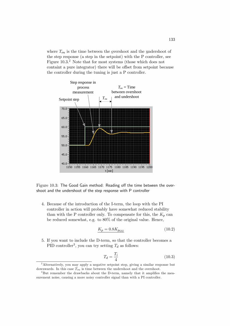
133

where Tou is the time between the overshoot and the undershoot ofthe step response (a step in the setpoint) with the P controller, seeFigure 10.3.2 Note that for most systems (those which does notcontaint a pure integrator) there will be offset from setpoint becausethe controller during the tuning is just a P controller.

TouSetpoint step

Step response in process

measurementTou = Time

between overshoot and undershoot

Figure 10.3: The Good Gain method: Reading off the time between the over-shoot and the undershoot of the step response with P controller

4. Because of the introduction of the I-term, the loop with the PIcontroller in action will probably have somewhat reduced stabilitythan with the P controller only. To compensate for this, the Kp canbe reduced somewhat, e.g. to 80% of the original value. Hence,

Kp = 0.8KpGG (10.2)

5. If you want to include the D-term, so that the controller becomes aPID controller3, you can try setting Td as follows:

Td =Ti4

(10.3)

2Alternatively, you may apply a negative setpoint step, giving a similar response butdownwards. In this case Tou is time between the undershoot and the overshoot.

3But remember the drawbacks about the D-term, namely that it amplifies the mea-surement noise, causing a more noisy controller signal than with a PI controller.

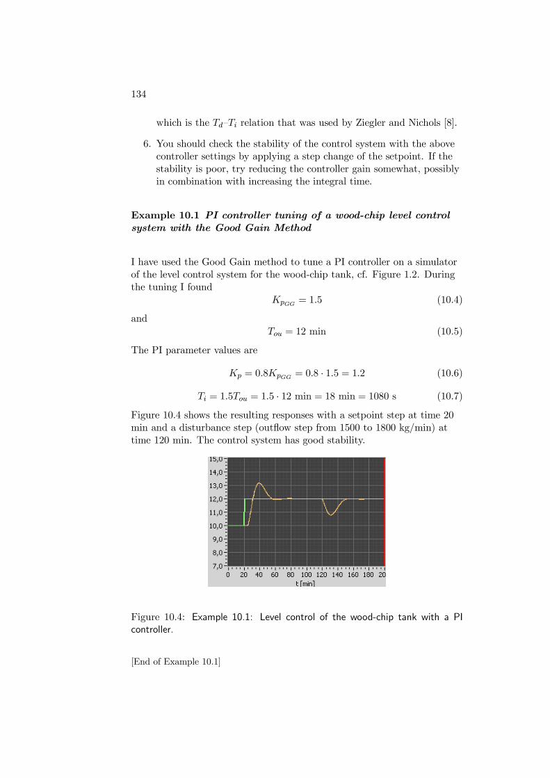
134

which is the Td—Ti relation that was used by Ziegler and Nichols [8].

6. You should check the stability of the control system with the abovecontroller settings by applying a step change of the setpoint. If thestability is poor, try reducing the controller gain somewhat, possiblyin combination with increasing the integral time.

Example 10.1 PI controller tuning of a wood-chip level controlsystem with the Good Gain Method

I have used the Good Gain method to tune a PI controller on a simulatorof the level control system for the wood-chip tank, cf. Figure 1.2. Duringthe tuning I found

KpGG = 1.5 (10.4)

andTou = 12 min (10.5)

The PI parameter values are

Kp = 0.8KpGG = 0.8 · 1.5 = 1.2 (10.6)

Ti = 1.5Tou = 1.5 · 12 min = 18 min = 1080 s (10.7)

Figure 10.4 shows the resulting responses with a setpoint step at time 20min and a disturbance step (outflow step from 1500 to 1800 kg/min) attime 120 min. The control system has good stability.

Figure 10.4: Example 10.1: Level control of the wood-chip tank with a PIcontroller.


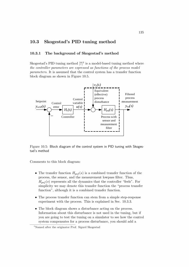
135

10.3 Skogestad’s PID tuning method

10.3.1 The background of Skogestad’s method

Skogestad’s PID tuning method [7]4 is a model-based tuning method wherethe controller parameters are expressed as functions of the process modelparameters. It is assumed that the control system has a transfer functionblock diagram as shown in Figure 10.5.

Hc(s) Hpsf(s)u(s) ymf(s)ymSP(s)

ve(s)

Process withsensor and

measurementfilter

Setpoint

Equivalent (effective)process disturbance

Filtered process

measurementControlerror

Controlvariable

Controller

Figure 10.5: Block diagram of the control system in PID tuning with Skoges-tad’s method

Comments to this block diagram:

• The transfer function Hpsf (s) is a combined transfer function of theprocess, the sensor, and the measurement lowpass filter. Thus,Hpsf (s) represents all the dynamics that the controller “feels”. Forsimplicity we may denote this transfer function the “process transferfunction”, although it is a combined transfer function.

• The process transfer function can stem from a simple step-responseexperiment with the process. This is explained in Sec. 10.3.3.

• The block diagram shows a disturbance acting on the process.Information about this disturbance is not used in the tuning, but ifyou are going to test the tuning on a simulator to see how the controlsystem compensates for a process disturbance, you should add a

4Named after the originator Prof. Sigurd Skogestad

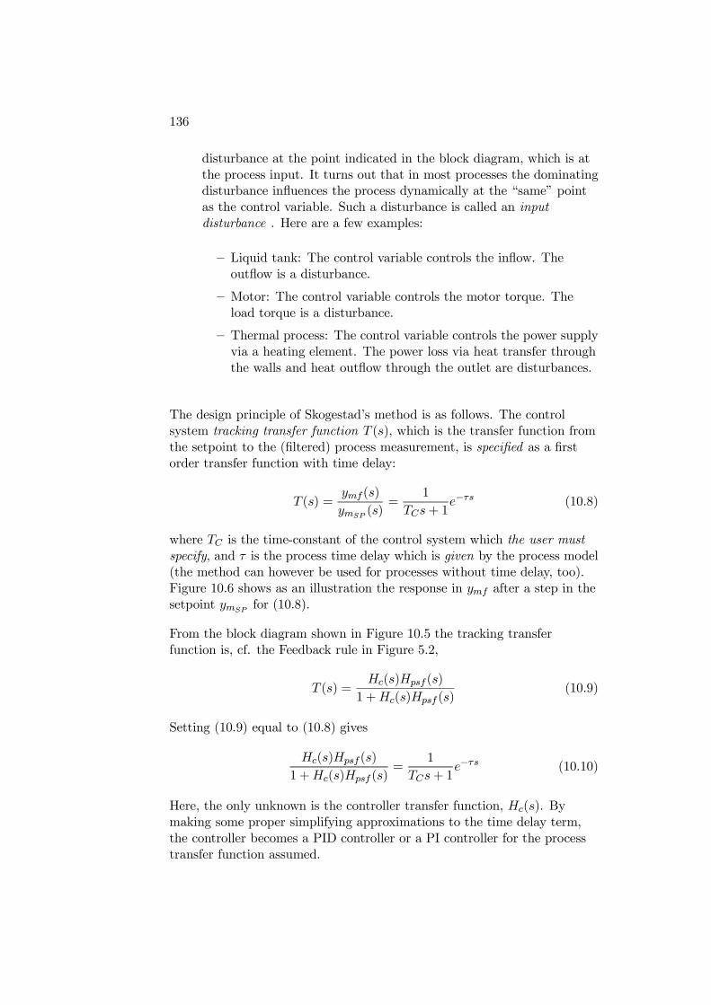
136

disturbance at the point indicated in the block diagram, which is atthe process input. It turns out that in most processes the dominatingdisturbance influences the process dynamically at the “same” pointas the control variable. Such a disturbance is called an inputdisturbance . Here are a few examples:

— Liquid tank: The control variable controls the inflow. Theoutflow is a disturbance.

— Motor: The control variable controls the motor torque. Theload torque is a disturbance.

— Thermal process: The control variable controls the power supplyvia a heating element. The power loss via heat transfer throughthe walls and heat outflow through the outlet are disturbances.

The design principle of Skogestad’s method is as follows. The controlsystem tracking transfer function T (s), which is the transfer function fromthe setpoint to the (filtered) process measurement, is specified as a firstorder transfer function with time delay:

T (s) =ymf (s)

ymSP(s)

=1

TCs+ 1e−τs (10.8)

where TC is the time-constant of the control system which the user mustspecify, and τ is the process time delay which is given by the process model(the method can however be used for processes without time delay, too).Figure 10.6 shows as an illustration the response in ymf after a step in thesetpoint ymSP

for (10.8).

From the block diagram shown in Figure 10.5 the tracking transferfunction is, cf. the Feedback rule in Figure 5.2,

T (s) =Hc(s)Hpsf (s)

1 +Hc(s)Hpsf (s)(10.9)

Setting (10.9) equal to (10.8) gives

Hc(s)Hpsf (s)

1 +Hc(s)Hpsf (s)=

1

TCs+ 1e−τs (10.10)

Here, the only unknown is the controller transfer function, Hc(s). Bymaking some proper simplifying approximations to the time delay term,the controller becomes a PID controller or a PI controller for the processtransfer function assumed.

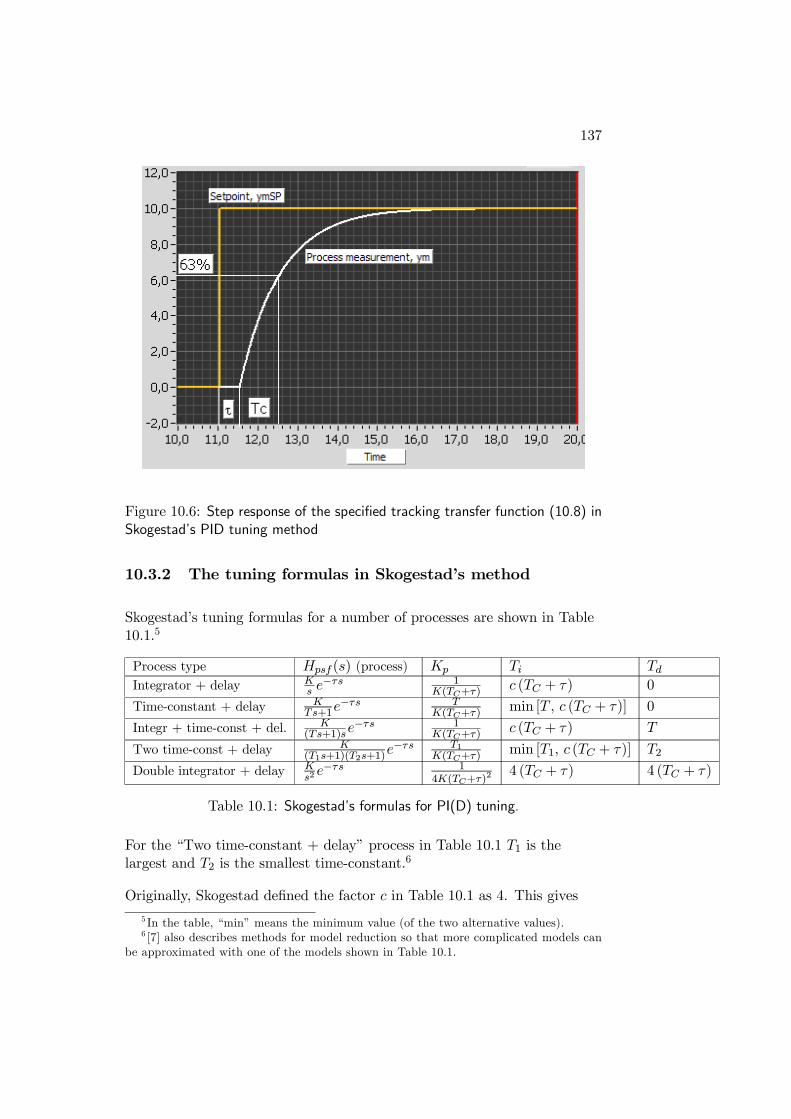
137

Figure 10.6: Step response of the specified tracking transfer function (10.8) inSkogestad’s PID tuning method

10.3.2 The tuning formulas in Skogestad’s method

Skogestad’s tuning formulas for a number of processes are shown in Table10.1.5

Process type Hpsf (s) (process) Kp Ti TdIntegrator + delay K

s e−τs 1

K(TC+τ)c (TC + τ) 0

Time-constant + delay KTs+1e

−τs TK(TC+τ)

min [T , c (TC + τ)] 0

Integr + time-const + del. K(Ts+1)se

−τs 1K(TC+τ)

c (TC + τ) T

Two time-const + delay K(T1s+1)(T2s+1)

e−τs T1K(TC+τ)

min [T1, c (TC + τ)] T2

Double integrator + delay Ks2e−τs 1

4K(TC+τ)2 4 (TC + τ) 4 (TC + τ)

Table 10.1: Skogestad’s formulas for PI(D) tuning.

For the “Two time-constant + delay” process in Table 10.1 T1 is thelargest and T2 is the smallest time-constant.6

Originally, Skogestad defined the factor c in Table 10.1 as 4. This gives

5 In the table, “min” means the minimum value (of the two alternative values).6 [7] also describes methods for model reduction so that more complicated models can

be approximated with one of the models shown in Table 10.1.

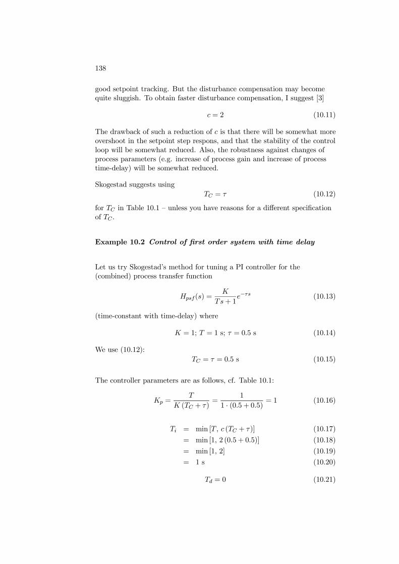
138

good setpoint tracking. But the disturbance compensation may becomequite sluggish. To obtain faster disturbance compensation, I suggest [3]

c = 2 (10.11)

The drawback of such a reduction of c is that there will be somewhat moreovershoot in the setpoint step respons, and that the stability of the controlloop will be somewhat reduced. Also, the robustness against changes ofprocess parameters (e.g. increase of process gain and increase of processtime-delay) will be somewhat reduced.

Skogestad suggests usingTC = τ (10.12)

for TC in Table 10.1 — unless you have reasons for a different specificationof TC .

Example 10.2 Control of first order system with time delay

Let us try Skogestad’s method for tuning a PI controller for the(combined) process transfer function

Hpsf (s) =K

Ts+ 1e−τs (10.13)

(time-constant with time-delay) where

K = 1; T = 1 s; τ = 0.5 s (10.14)

We use (10.12):TC = τ = 0.5 s (10.15)

The controller parameters are as follows, cf. Table 10.1:

Kp =T

K (TC + τ)=

1

1 · (0.5 + 0.5)= 1 (10.16)

Ti = min [T , c (TC + τ)] (10.17)

= min [1, 2 (0.5 + 0.5)] (10.18)

= min [1, 2] (10.19)

= 1 s (10.20)

Td = 0 (10.21)

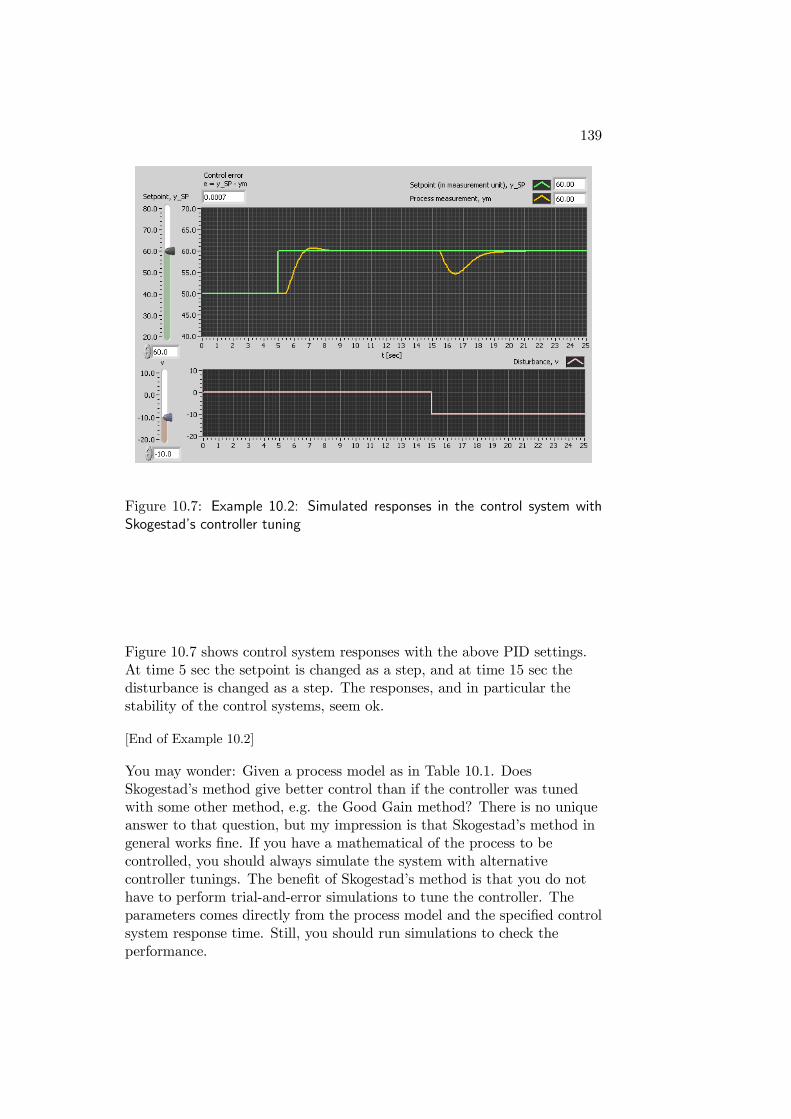
139

Figure 10.7: Example 10.2: Simulated responses in the control system withSkogestad’s controller tuning

Figure 10.7 shows control system responses with the above PID settings.At time 5 sec the setpoint is changed as a step, and at time 15 sec thedisturbance is changed as a step. The responses, and in particular thestability of the control systems, seem ok.


You may wonder: Given a process model as in Table 10.1. DoesSkogestad’s method give better control than if the controller was tunedwith some other method, e.g. the Good Gain method? There is no uniqueanswer to that question, but my impression is that Skogestad’s method ingeneral works fine. If you have a mathematical of the process to becontrolled, you should always simulate the system with alternativecontroller tunings. The benefit of Skogestad’s method is that you do nothave to perform trial-and-error simulations to tune the controller. Theparameters comes directly from the process model and the specified controlsystem response time. Still, you should run simulations to check theperformance.

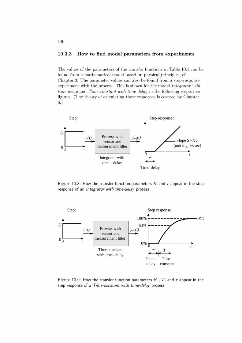
140

10.3.3 How to find model parameters from experiments

The values of the parameters of the transfer functions in Table 10.1 can befound from a mathematical model based on physical principles, cf.Chapter 3. The parameter values can also be found from a step-responseexperiment with the process. This is shown for the model Integrator withtime-delay and Time-constant with time-delay in the following respectivefigures. (The theory of calculating these responses is covered by Chapter6.)

Prosess with sensor and

measurement filter

U

0 t0

t0

Slope S=KU(unit e.g. %/sec)

u(t) ymf(t)

Step: Step response :

Time-delay

Integrator withtime - delay

Figure 10.8: How the transfer function parameters K and τ appear in the stepresponse of an Integrator with time-delay prosess

Prosess with sensor and

measurement filter

U

0 t0

T0

KU

u(t) ymf(t)

Step: Step response :

Time-delay

Time-constant with time-delay

Time-constant

63%

100%

0%t

Figure 10.9: How the transfer function parameters K , T , and τ appear in thestep response of a Time-constant with time-delay prosess

141

10.3.4 Transformation from serial to parallel PID settings

Skogestad’s formulas assumes a serial PID controller function(alternatively denoted cascade PID controller) which has the followingtransfer function:

u(s) = Kps(Tiss+ 1) (Tdss+ 1)

Tisse(s) (10.22)

where Kps , Tis , and Tds are the controller parameters. If your controlleractually implementes a parallel PID controller (as in the PID controllers inLabVIEW PID Control Toolkit and in the Matlab/Simulink PIDcontrollers), which has the following transfer function:

u(s) =

Kpp +

KppTips

+KppTdps

e(s) (10.23)

then you should transform from serial PID settings to parallell PIDsettings. If you do not implement these transformations, the controlsystem may behave unnecessarily different from the specified response.The serial-to-parallel transformations are as follows:

Kpp = Kps

1 +

TdsTis

(10.24)

Tip = Tis

1 +

TdsTis

(10.25)

Tdp = Tds1

1 +TdsTis

(10.26)

Note: The parallel and serial PI controllers are identical (since Td = 0 in aPI controller). Therefore, the above transformations are not relevant for PIcontroller, only for PID controllers.

10.3.5 When the process has no time-delay

What if the process Hp(s) is without time-delay? Then you can not specifyTC according to (10.12) since that would give TC = 0 (zero response timeof the control system). You must specify TC to some reasonable valuelarger than zero. If you do not know what could be a reasonable value, youcan simulate the control system for various values of TC . If the controlsignal (controller output signal) is changing too quickly, or often reachesthe maximum and minimum values for reasonable changes of the setpoint

142

or the disturbance, the controller is too aggressive, and you can tryincreasing TC . If you don’t want to simulate, then just try settingTC = T/2 where T is the dominating (largest) time-constant of the process(assuming the process is a time-constant system, of course).

For the double integrator (without time-delay) I have seen in simulationsthat the actual response-time (or 63% rise-time) of the closed-loop systemmay be about twice the specified time-constantTC . Consequently, you canset TC to about half of the response-time you actually want to obtain.

10.4 Auto-tuning

Auto-tuning is automatic tuning of controller parameters in oneexperiment. It is common that commercial controllers offers auto-tuning.The operator starts the auto-tuning via some button or menu choice onthe controller. The controller then executes automatically a pre-plannedexperiment on the uncontrolled process or on the control system dependingon the auto-tuning method implemented. Below are described a couple ofauto-tuning methods.

Auto-tuning based on relay tuning

The relay method for tuning PID controllers is used as the basis ofauto-tuning in some commercial controllers.7 The principle of this methodis as follows: When the auto-tuning phase is started, a relay controller isused as the controller in the control loop, see Figure 10.10. The relaycontroller is simply an On/Off controller. It sets the control signal to ahigh (On) value when the control error is positive, and to a low (Off) valuewhen the control error is negative. This controller creates automaticallysustained oscillations in control loop, and from the amplitude and theperiod of these oscillations proper PID controller parameters are calculatedby an algorithm in the controller. Only a few periods are needed for theautotuner to have enough information to accomplish the tuning. Theautotuner activates the tuned PID controller automatically after thetuning has finished.

7For example the ABB ECA600 PID controller and the Fuji PGX PID controller.

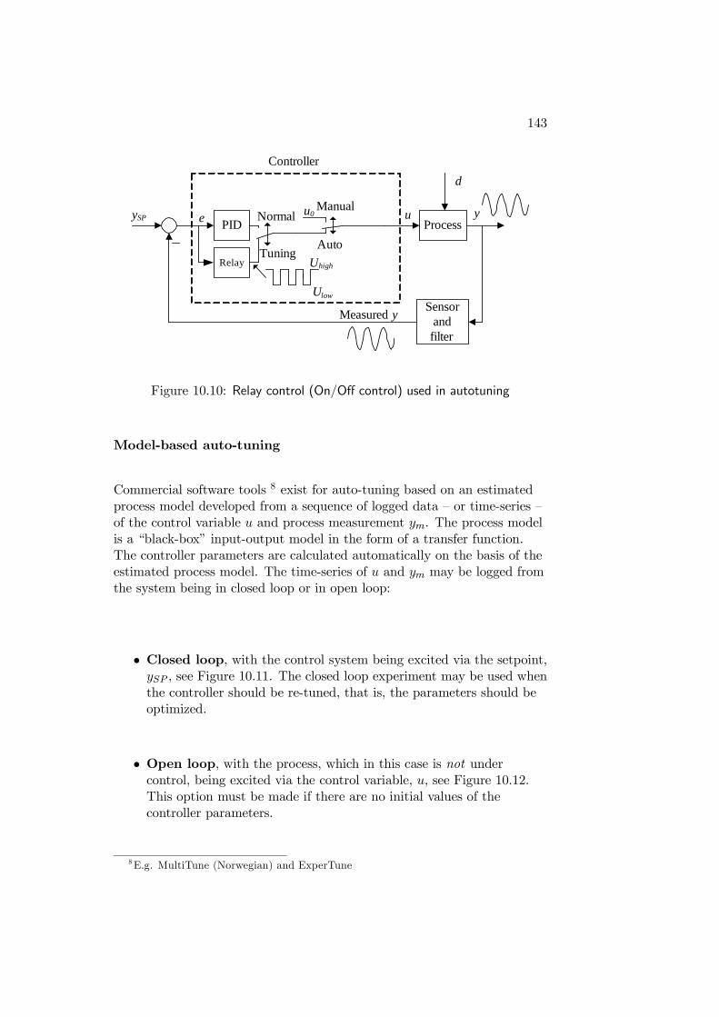
143

Process

Sensorand filter

d

y

Measured y

ySP ue PIDu0

Auto

Manual

Controller

RelayTuning

Normal

Uhigh

Ulow

Figure 10.10: Relay control (On/Off control) used in autotuning

Model-based auto-tuning

Commercial software tools 8 exist for auto-tuning based on an estimatedprocess model developed from a sequence of logged data — or time-series —of the control variable u and process measurement ym. The process modelis a “black-box” input-output model in the form of a transfer function.The controller parameters are calculated automatically on the basis of theestimated process model. The time-series of u and ym may be logged fromthe system being in closed loop or in open loop:

• Closed loop, with the control system being excited via the setpoint,ySP , see Figure 10.11. The closed loop experiment may be used whenthe controller should be re-tuned, that is, the parameters should beoptimized.

• Open loop, with the process, which in this case is not undercontrol, being excited via the control variable, u, see Figure 10.12.This option must be made if there are no initial values of thecontroller parameters.

8E.g. MultiTune (Norwegian) and ExperTune

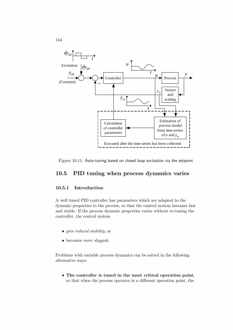
144

Executed after the time-series has been collected

Process

Sensorand

scaling

yySP uController

ym

Estimation ofprocess model

from time-seriesof u and ym

Calculationof controllerparameters

dySP

tdySP

t

ym

(Constant)

t

uExcitation

Figure 10.11: Auto-tuning based on closed loop excitation via the setpoint

10.5 PID tuning when process dynamics varies

10.5.1 Introduction

A well tuned PID controller has parameters which are adapted to thedynamic properties to the process, so that the control system becomes fastand stable. If the process dynamic properties varies without re-tuning thecontroller, the control system

• gets reduced stability, or

• becomes more sluggish.

Problems with variable process dynamics can be solved in the followingalternative ways:

• The controller is tuned in the most critical operation point,so that when the process operates in a different operation point, the

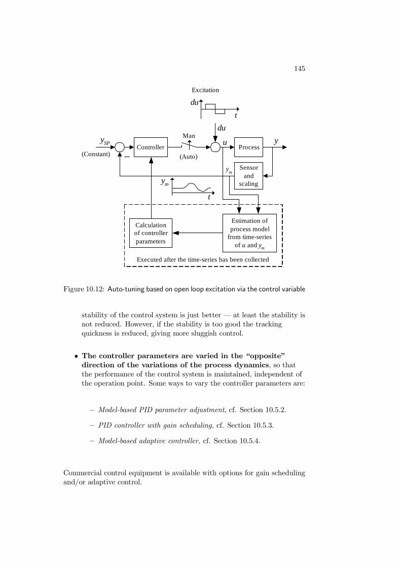
145

ProcessyySP u

Controller

ym

Estimation ofprocess model

from time-seriesof u and ym

Calculationof controllerparameters

duMan

(Auto)

t

du

t

ym

(Constant)

Executed after the time-series has been collected

Excitation

Sensorand

scaling

Figure 10.12: Auto-tuning based on open loop excitation via the control variable

stability of the control system is just better – at least the stability isnot reduced. However, if the stability is too good the trackingquickness is reduced, giving more sluggish control.

• The controller parameters are varied in the “opposite”direction of the variations of the process dynamics, so thatthe performance of the control system is maintained, independent ofthe operation point. Some ways to vary the controller parameters are:

— Model-based PID parameter adjustment, cf. Section 10.5.2.

— PID controller with gain scheduling, cf. Section 10.5.3.

— Model-based adaptive controller, cf. Section 10.5.4.

Commercial control equipment is available with options for gain schedulingand/or adaptive control.

146

10.5.2 PID parameter adjustment with Skogestad’s method

Assume that you have tuned a PID or a PI controller for some process thathas a transfer function equal to one of the transfer functions Hpsf (s) shownin Table 10.1. Assume then that some of the parameters of the processtransfer function changes. How should the controller parameters beadjusted? The answer is given by Table 10.1 because it gives the controllerparameters as functions of the process parameters. You can actually usethis table as the basis for adjusting the PID parameters even if you usedsome other method than Skogestad’s method for the initial tuning.

From Table 10.1 we can draw a number of general rules for adjusting thePID parameters:

Example 10.3 Adjustment of PI controller parameters forintegrator with time delay process

Assume that the process transfer function is

Hpsf (s) =K

se−τs (10.27)

(integrator with time delay). According to Table 10.1, with the suggestedspecification TC = τ , the PI controller parameters are

Kp =1

2Kτ(10.28)

Ti = k12τ (10.29)

As an example, assume that the process gain K is increased to, say, twiceits original value. How should the PI parameters be adjusted to maintaingood behaviour of the control system? From (10.28) we see that Kp shouldbe halved, and from (10.29) we see that Ti should remain unchanged.

As another example, assume that the process time delay τ is increased to,say, twice its original value. From (10.28) we see that Kp should be halved,and from (10.29) we see that Ti should get a doubled value. One concreteexample of such a process change is the wood-chip tank. If the speed ofthe conveyor belt is halved, the time delay (transport delay) is doubled.And now you know how to quickly adjust the PI controller parameters ifsuch a change of the conveyor belt speed should occur.9

[End of Example 10.3]9What may happen if you do not adjust the controller parameters? The control system

may get poor stability, or it may even become unstable.

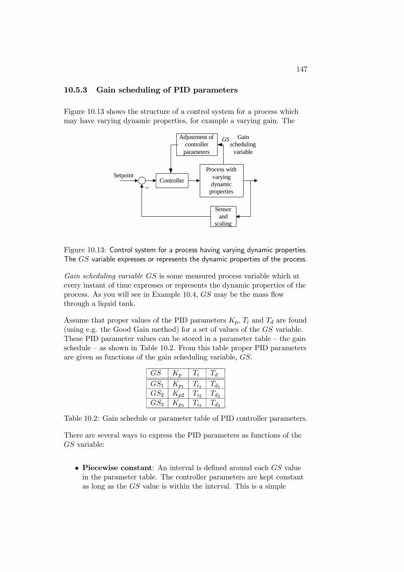
147

10.5.3 Gain scheduling of PID parameters

Figure 10.13 shows the structure of a control system for a process whichmay have varying dynamic properties, for example a varying gain. The

Process withvaryingdynamicproperties

Sensorand

scaling

SetpointController

Adjustment ofcontrollerparameters

GS Gainscheduling

variable

Figure 10.13: Control system for a process having varying dynamic properties.The GS variable expresses or represents the dynamic properties of the process.

Gain scheduling variable GS is some measured process variable which atevery instant of time expresses or represents the dynamic properties of theprocess. As you will see in Example 10.4, GS may be the mass flowthrough a liquid tank.

Assume that proper values of the PID parameters Kp, Ti and Td are found(using e.g. the Good Gain method) for a set of values of the GS variable.These PID parameter values can be stored in a parameter table — the gainschedule — as shown in Table 10.2. From this table proper PID parametersare given as functions of the gain scheduling variable, GS.

GS Kp Ti Td

GS1 Kp1 Ti1 Td1GS2 Kp2 Ti2 Td2GS3 Kp3 Ti3 Td3

Table 10.2: Gain schedule or parameter table of PID controller parameters.

There are several ways to express the PID parameters as functions of theGS variable:

• Piecewise constant: An interval is defined around each GS valuein the parameter table. The controller parameters are kept constantas long as the GS value is within the interval. This is a simple

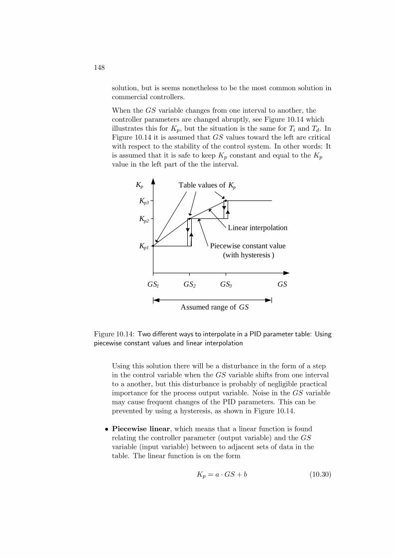
148

solution, but is seems nonetheless to be the most common solution incommercial controllers.

When the GS variable changes from one interval to another, thecontroller parameters are changed abruptly, see Figure 10.14 whichillustrates this for Kp, but the situation is the same for Ti and Td. InFigure 10.14 it is assumed that GS values toward the left are criticalwith respect to the stability of the control system. In other words: Itis assumed that it is safe to keep Kp constant and equal to the Kp

value in the left part of the the interval.

GS1 GS2 GS3 GS

Kp1

Kp2

Kp3

Kp

Assumed range of GS

Table values of Kp

Linear interpolation

Piecewise constant value (with hysteresis )

Figure 10.14: Two different ways to interpolate in a PID parameter table: Usingpiecewise constant values and linear interpolation

Using this solution there will be a disturbance in the form of a stepin the control variable when the GS variable shifts from one intervalto a another, but this disturbance is probably of negligible practicalimportance for the process output variable. Noise in the GS variablemay cause frequent changes of the PID parameters. This can beprevented by using a hysteresis, as shown in Figure 10.14.

• Piecewise linear, which means that a linear function is foundrelating the controller parameter (output variable) and the GSvariable (input variable) between to adjacent sets of data in thetable. The linear function is on the form

Kp = a ·GS + b (10.30)

149

where a and b are found from the two corresponding data sets:

Kp1 = a ·GS1 + b (10.31)

Kp2 = a ·GS2 + b (10.32)

(Similar equations applies to the Ti parameter and the Tdparameter.) (10.31) and (10.32) constitute a set of two equationswith two unknown variables, a and b (the solution is left to you).10

• Other interpolations may be used, too, for example a polynomialfunction fitted exactly to the data or fitted using the least squaresmethod.

Example 10.4 PID temperature control with gain schedulingduring variable mass flow

Figure 10.16 shows the front panel of a simulator for a temperature controlsystem for a liquid tank with variable mass flow, w, through the tank. Thecontrol variable u controls the power to heating element. The temperatureT is measured by a sensor which is placed some distance away from theheating element. There is a time delay from the control variable tomeasurement due to imperfect blending in the tank.

The process dynamics

We will initially, both in simulations and from analytical expressions, thatthe dynamic properties of the process varies with the mass flow w. Theresponse in the temperature T after a step change in the control signal(which is proportional to the supplied power) is simulated for a large massflow and a small mass flow. (Feedback temperature control is not active,thus open loop responses are shown.) The responses are shown in Figure10.15. The simulations show that the following happens when the massflow w is reduced (from 24 to 12 kg/min): The gain process K is larger. Itcan be shown that in addition, the time-constant Tt is larger, and the timedelay τ is larger. (These terms assumes that system is a first order systemwith time delay. The simulator is based on such a model. The model isdescribed below.)

Let us see if the way the process dynamics seems to depend on the massflow w as seen from the simulations, can be confirmed from a

10Note that both MATLAB/SIMULINK and LabVIEW have functions that implementlinear interpolation between tabular data. Therefore gain scheduling can be easily imple-mented in these environments.

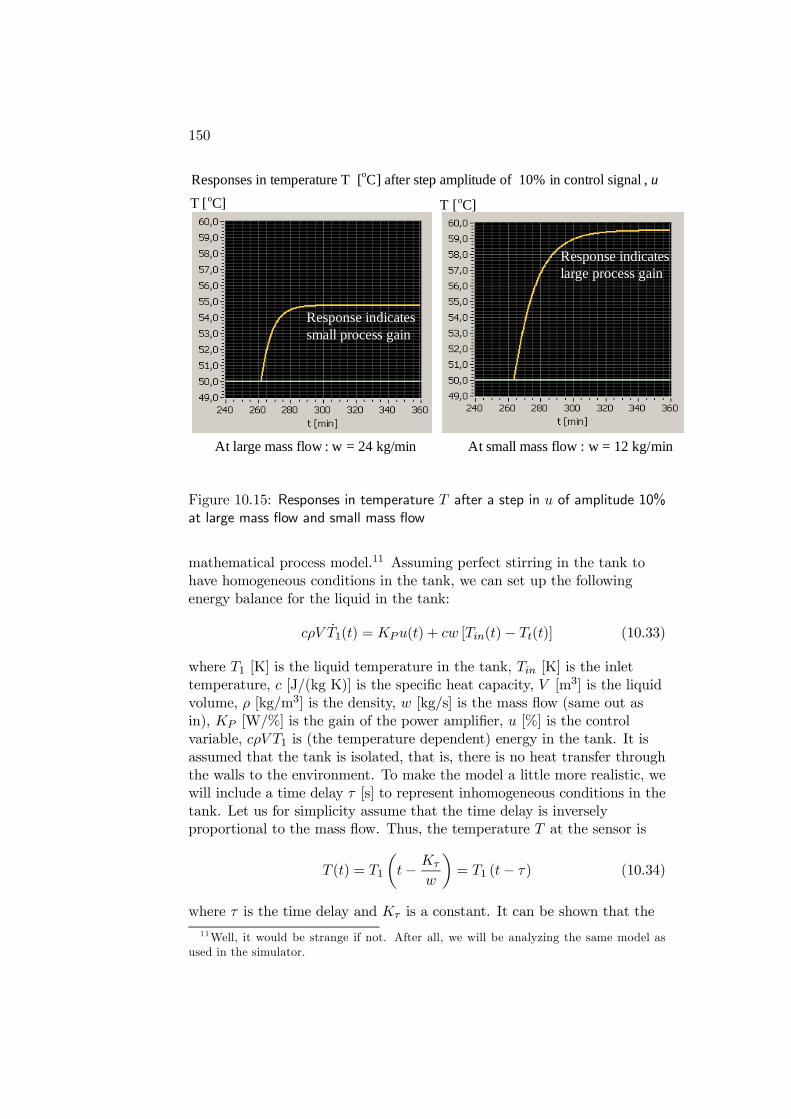
150

At large mass flow : w = 24 kg/min

Responses in temperature T [oC] after step amplitude of 10% in control signal , u

T [oC]

At small mass flow : w = 12 kg/min

T [oC]

Response indicates small process gain

Response indicates large process gain

Figure 10.15: Responses in temperature T after a step in u of amplitude 10%at large mass flow and small mass flow

mathematical process model.11 Assuming perfect stirring in the tank tohave homogeneous conditions in the tank, we can set up the followingenergy balance for the liquid in the tank:

cρV T1(t) = KPu(t) + cw [Tin(t)− Tt(t)] (10.33)

where T1 [K] is the liquid temperature in the tank, Tin [K] is the inlettemperature, c [J/(kg K)] is the specific heat capacity, V [m3] is the liquidvolume, ρ [kg/m3] is the density, w [kg/s] is the mass flow (same out asin), KP [W/%] is the gain of the power amplifier, u [%] is the controlvariable, cρV T1 is (the temperature dependent) energy in the tank. It isassumed that the tank is isolated, that is, there is no heat transfer throughthe walls to the environment. To make the model a little more realistic, wewill include a time delay τ [s] to represent inhomogeneous conditions in thetank. Let us for simplicity assume that the time delay is inverselyproportional to the mass flow. Thus, the temperature T at the sensor is

T (t) = T1

t−

Kτw

= T1 (t− τ) (10.34)

where τ is the time delay and Kτ is a constant. It can be shown that the11Well, it would be strange if not. After all, we will be analyzing the same model as

used in the simulator.

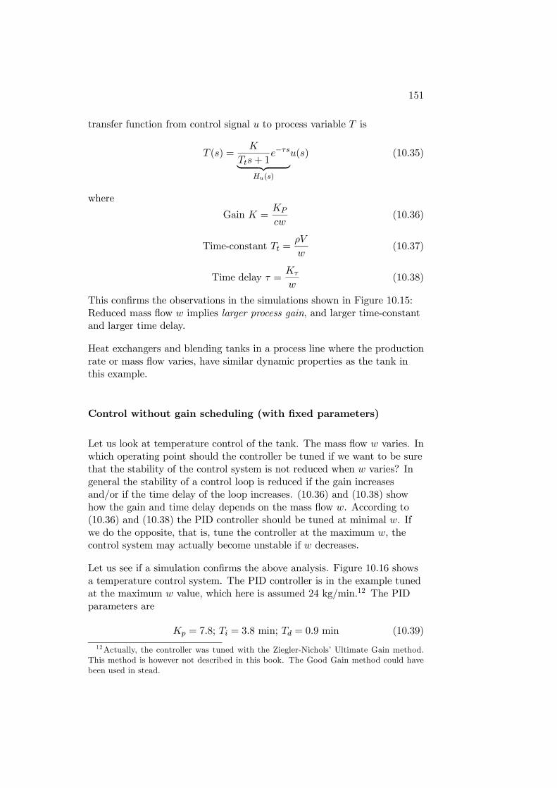
151

transfer function from control signal u to process variable T is

T (s) =K

Tts+ 1e−τs

Hu(s)

u(s) (10.35)

where

Gain K =KPcw

(10.36)

Time-constant Tt =ρV

w(10.37)

Time delay τ =Kτw

(10.38)

This confirms the observations in the simulations shown in Figure 10.15:Reduced mass flow w implies larger process gain, and larger time-constantand larger time delay.

Heat exchangers and blending tanks in a process line where the productionrate or mass flow varies, have similar dynamic properties as the tank inthis example.

Control without gain scheduling (with fixed parameters)

Let us look at temperature control of the tank. The mass flow w varies. Inwhich operating point should the controller be tuned if we want to be surethat the stability of the control system is not reduced when w varies? Ingeneral the stability of a control loop is reduced if the gain increasesand/or if the time delay of the loop increases. (10.36) and (10.38) showhow the gain and time delay depends on the mass flow w. According to(10.36) and (10.38) the PID controller should be tuned at minimal w. Ifwe do the opposite, that is, tune the controller at the maximum w, thecontrol system may actually become unstable if w decreases.

Let us see if a simulation confirms the above analysis. Figure 10.16 showsa temperature control system. The PID controller is in the example tunedat the maximum w value, which here is assumed 24 kg/min.12 The PIDparameters are

Kp = 7.8; Ti = 3.8 min; Td = 0.9 min (10.39)

12Actually, the controller was tuned with the Ziegler-Nichols’ Ultimate Gain method.This method is however not described in this book. The Good Gain method could havebeen used in stead.

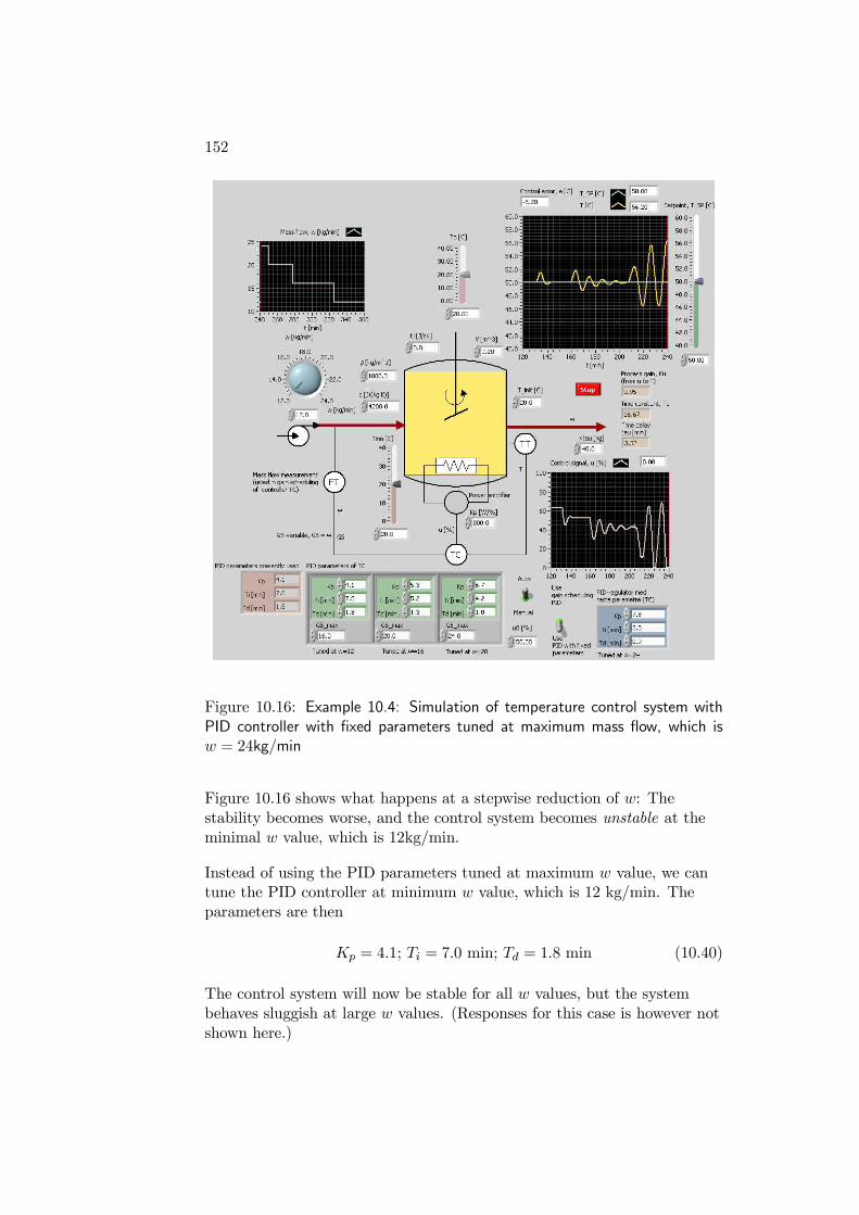
152

Figure 10.16: Example 10.4: Simulation of temperature control system withPID controller with fixed parameters tuned at maximum mass flow, which isw = 24kg/min

Figure 10.16 shows what happens at a stepwise reduction of w: Thestability becomes worse, and the control system becomes unstable at theminimal w value, which is 12kg/min.

Instead of using the PID parameters tuned at maximum w value, we cantune the PID controller at minimum w value, which is 12 kg/min. Theparameters are then

Kp = 4.1; Ti = 7.0 min; Td = 1.8 min (10.40)

The control system will now be stable for all w values, but the systembehaves sluggish at large w values. (Responses for this case is however notshown here.)

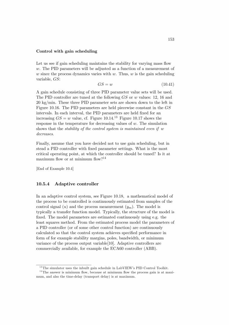
153

Control with gain scheduling

Let us see if gain scheduling maintains the stability for varying mass floww. The PID parameters will be adjusted as a function of a measurement ofw since the process dynamics varies with w. Thus, w is the gain schedulingvariable, GS:

GS = w (10.41)

A gain schedule consisting of three PID parameter value sets will be used.The PID controller are tuned at the following GS or w values: 12, 16 and20 kg/min. These three PID parameter sets are shown down to the left inFigure 10.16. The PID parameters are held piecewise constant in the GSintervals. In each interval, the PID parameters are held fixed for anincreasing GS = w value, cf. Figure 10.14.13 Figure 10.17 shows theresponse in the temperature for decreasing values of w. The simulationshows that the stability of the control system is maintained even if wdecreases.

Finally, assume that you have decided not to use gain scheduling, but instead a PID controller with fixed parameter settings. What is the mostcritical operating point, at which the controller should be tuned? Is it atmaximum flow or at minimum flow?14


10.5.4 Adaptive controller

In an adaptive control system, see Figure 10.18, a mathematical model ofthe process to be controlled is continuously estimated from samples of thecontrol signal (u) and the process measurement (ym). The model istypically a transfer function model. Typically, the structure of the model isfixed. The model parameters are estimated continuously using e.g. theleast squares method. From the estimated process model the parameters ofa PID controller (or of some other control function) are continuouslycalculated so that the control system achieves specified performance inform of for example stability margins, poles, bandwidth, or minimumvariance of the process output variable[10]. Adaptive controllers arecommercially available, for example the ECA60 controller (ABB).

13The simulator uses the inbuilt gain schedule in LabVIEW’s PID Control Toolkit.14The answer is minimum flow, because at minimum flow the process gain is at maxi-

mum, and also the time-delay (transport delay) is at maximum.

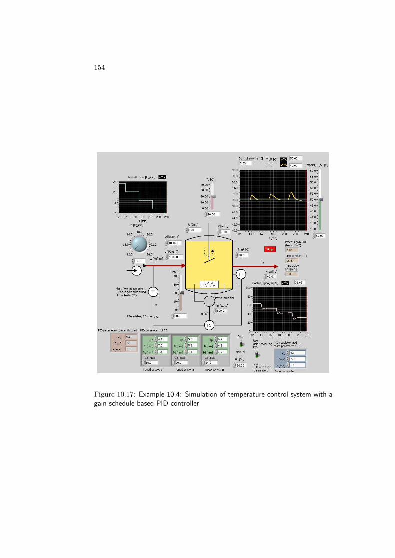
154

Figure 10.17: Example 10.4: Simulation of temperature control system with again schedule based PID controller

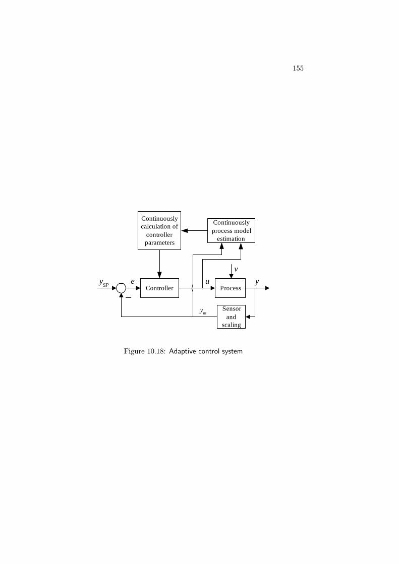
155

Process

Sensorand

scaling

v

yySP

ueController

ym

Continuouslyprocess model

estimation

Continuouslycalculation of

controllerparameters

Figure 10.18: Adaptive control system

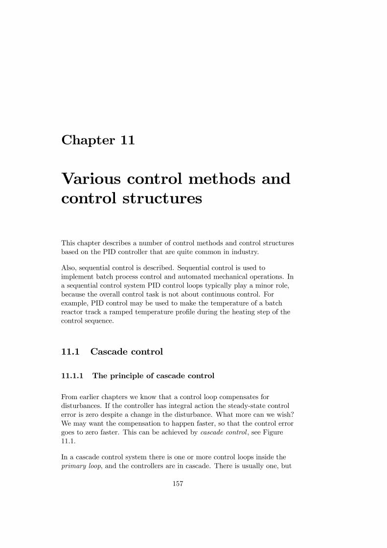
Chapter 11

Various control methods andcontrol structures

This chapter describes a number of control methods and control structuresbased on the PID controller that are quite common in industry.

Also, sequential control is described. Sequential control is used toimplement batch process control and automated mechanical operations. Ina sequential control system PID control loops typically play a minor role,because the overall control task is not about continuous control. Forexample, PID control may be used to make the temperature of a batchreactor track a ramped temperature profile during the heating step of thecontrol sequence.

11.1 Cascade control

11.1.1 The principle of cascade control

From earlier chapters we know that a control loop compensates fordisturbances. If the controller has integral action the steady-state controlerror is zero despite a change in the disturbance. What more can we wish?We may want the compensation to happen faster, so that the control errorgoes to zero faster. This can be achieved by cascade control , see Figure11.1.

In a cascade control system there is one or more control loops inside theprimary loop, and the controllers are in cascade. There is usually one, but

157

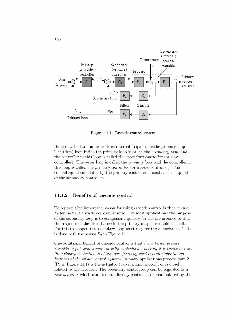
158

Figure 11.1: Cascade control system

there may be two and even three internal loops inside the primary loop.The (first) loop inside the primary loop is called the secondary loop, andthe controller in this loop is called the secondary controller (or slavecontroller). The outer loop is called the primary loop, and the controller inthis loop is called the primary controller (or master-controller). Thecontrol signal calculated by the primary controller is used as the setpointof the secondary controller.

11.1.2 Benefits of cascade control

To repeat: One important reason for using cascade control is that it givesfaster (better) disturbance compensation. In most applications the purposeof the secondary loop is to compensate quickly for the disturbance so thatthe response of the disturbance in the primary output variable is small.For this to happen the secondary loop must register the disturbance. Thisis done with the sensor S2 in Figure 11.1.

One additional benefit of cascade control is that the internal processvariable ( y2) becomes more directly controllable, making it is easier to tunethe primary controller to obtain satisfactorily good overall stability andfastness of the whole control system. In many applications process part 2(P2 in Figure 11.1) is the actuator (valve, pump, motor), or is closelyrelated to the actuator. The secondary control loop can be regarded as anew actuator which can be more directly controlled or manipulated by the

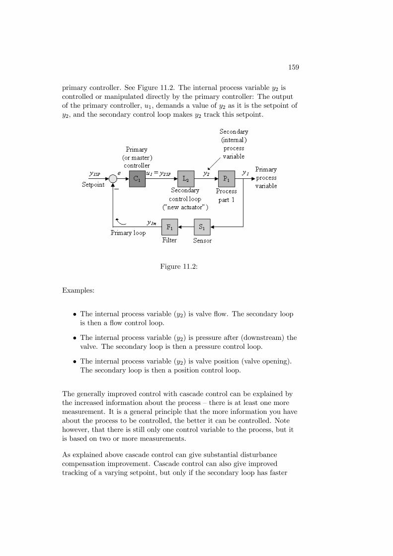
159

primary controller. See Figure 11.2. The internal process variable y2 iscontrolled or manipulated directly by the primary controller: The outputof the primary controller, u1, demands a value of y2 as it is the setpoint ofy2, and the secondary control loop makes y2 track this setpoint.

Figure 11.2:

Examples:

• The internal process variable (y2) is valve flow. The secondary loopis then a flow control loop.

• The internal process variable (y2) is pressure after (downstream) thevalve. The secondary loop is then a pressure control loop.

• The internal process variable (y2) is valve position (valve opening).The secondary loop is then a position control loop.

The generally improved control with cascade control can be explained bythe increased information about the process — there is at least one moremeasurement. It is a general principle that the more information you haveabout the process to be controlled, the better it can be controlled. Notehowever, that there is still only one control variable to the process, but itis based on two or more measurements.

As explained above cascade control can give substantial disturbancecompensation improvement. Cascade control can also give improvedtracking of a varying setpoint, but only if the secondary loop has faster

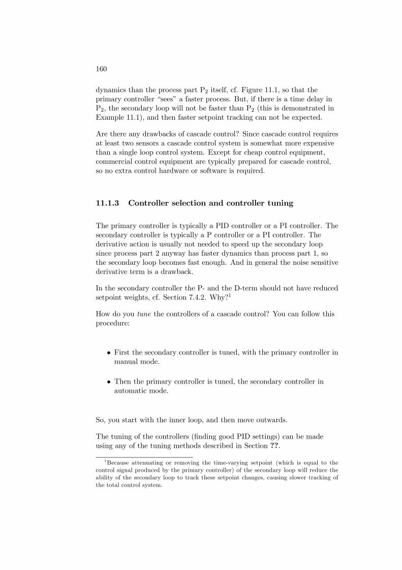
160

dynamics than the process part P2 itself, cf. Figure 11.1, so that theprimary controller “sees” a faster process. But, if there is a time delay inP2, the secondary loop will not be faster than P2 (this is demonstrated inExample 11.1), and then faster setpoint tracking can not be expected.

Are there any drawbacks of cascade control? Since cascade control requiresat least two sensors a cascade control system is somewhat more expensivethan a single loop control system. Except for cheap control equipment,commercial control equipment are typically prepared for cascade control,so no extra control hardware or software is required.

11.1.3 Controller selection and controller tuning

The primary controller is typically a PID controller or a PI controller. Thesecondary controller is typically a P controller or a PI controller. Thederivative action is usually not needed to speed up the secondary loopsince process part 2 anyway has faster dynamics than process part 1, sothe secondary loop becomes fast enough. And in general the noise sensitivederivative term is a drawback.

In the secondary controller the P- and the D-term should not have reducedsetpoint weights, cf. Section 7.4.2. Why?1

How do you tune the controllers of a cascade control? You can follow thisprocedure:

• First the secondary controller is tuned, with the primary controller inmanual mode.

• Then the primary controller is tuned, the secondary controller inautomatic mode.

So, you start with the inner loop, and then move outwards.

The tuning of the controllers (finding good PID settings) can be madeusing any of the tuning methods described in Section ??.

1Because attenuating or removing the time-varying setpoint (which is equal to thecontrol signal produced by the primary controller) of the secondary loop will reduce theability of the secondary loop to track these setpoint changes, causing slower tracking ofthe total control system.

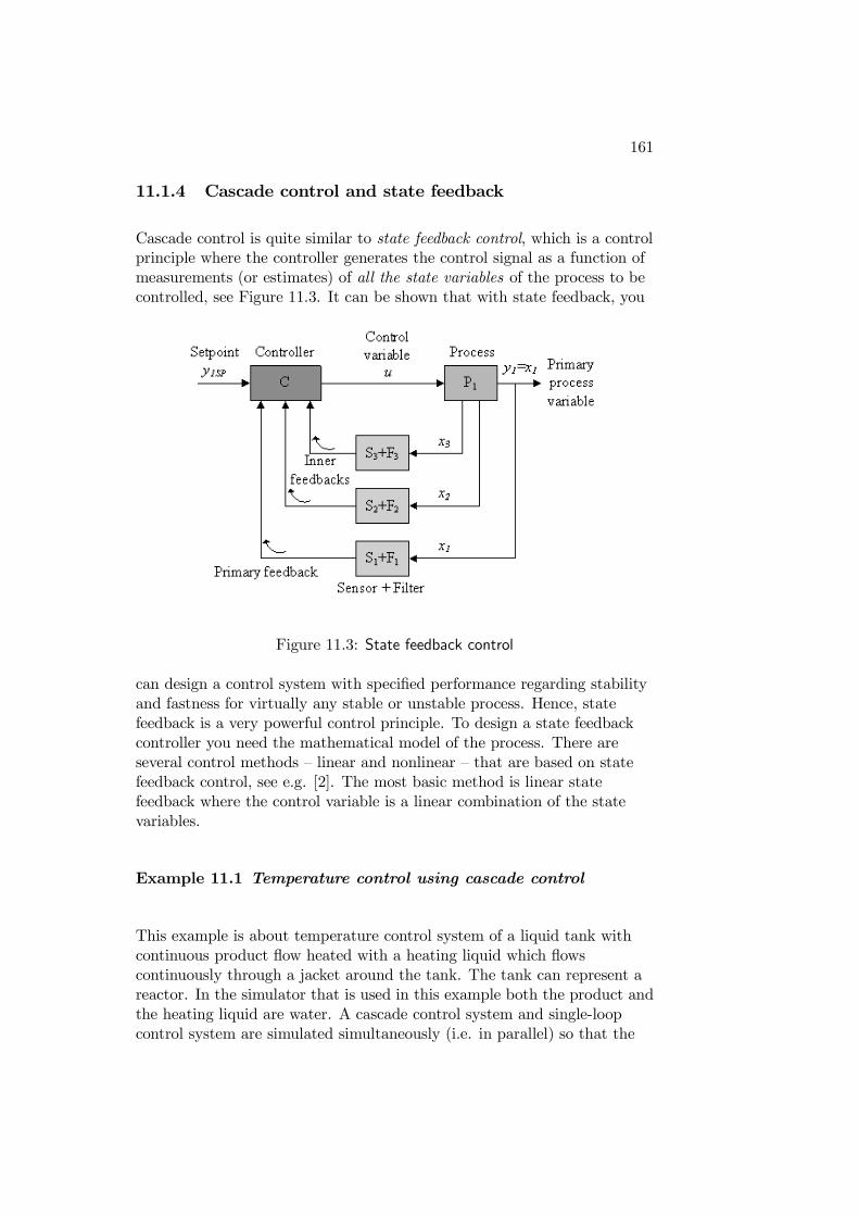
161

11.1.4 Cascade control and state feedback

Cascade control is quite similar to state feedback control, which is a controlprinciple where the controller generates the control signal as a function ofmeasurements (or estimates) of all the state variables of the process to becontrolled, see Figure 11.3. It can be shown that with state feedback, you

Figure 11.3: State feedback control

can design a control system with specified performance regarding stabilityand fastness for virtually any stable or unstable process. Hence, statefeedback is a very powerful control principle. To design a state feedbackcontroller you need the mathematical model of the process. There areseveral control methods — linear and nonlinear — that are based on statefeedback control, see e.g. [2]. The most basic method is linear statefeedback where the control variable is a linear combination of the statevariables.

Example 11.1 Temperature control using cascade control

This example is about temperature control system of a liquid tank withcontinuous product flow heated with a heating liquid which flowscontinuously through a jacket around the tank. The tank can represent areactor. In the simulator that is used in this example both the product andthe heating liquid are water. A cascade control system and single-loopcontrol system are simulated simultaneously (i.e. in parallel) so that the

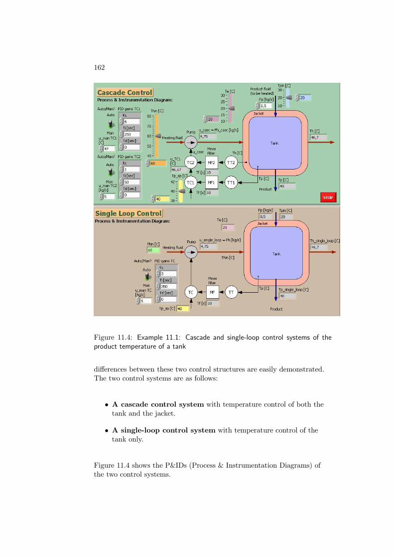
162

Figure 11.4: Example 11.1: Cascade and single-loop control systems of theproduct temperature of a tank

differences between these two control structures are easily demonstrated.The two control systems are as follows:

• A cascade control system with temperature control of both thetank and the jacket.

• A single-loop control system with temperature control of thetank only.

Figure 11.4 shows the P&IDs (Process & Instrumentation Diagrams) ofthe two control systems.

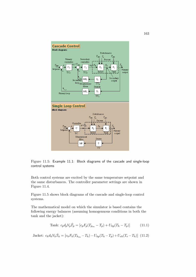
163

Figure 11.5: Example 11.1: Block diagrams of the cascade and single-loopcontrol systems

Both control systems are excited by the same temperature setpoint andthe same disturbances. The controller parameter settings are shown inFigure 11.4.

Figure 11.5 shows block diagrams of the cascade and single-loop controlsystems.

The mathematical model on which the simulator is based contains thefollowing energy balances (assuming homogenuous conditions in both thetank and the jacket):

Tank: cpdpVpTp = [cpFp(Tpin − Tp) + Uhp(Th − Tp)] (11.1)

Jacket: chdhVhTh = [chFh(Thin −Th)−Uhp(Th−Tp)+Ueh(Te−Th)] (11.2)

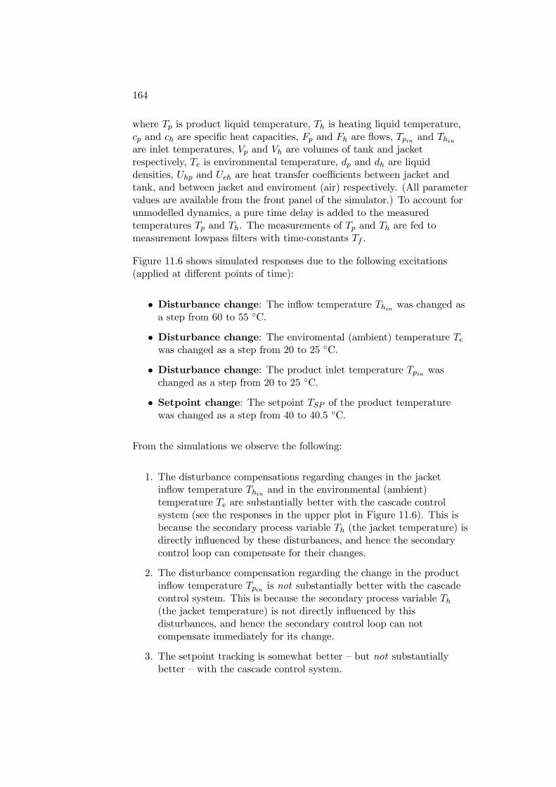
164

where Tp is product liquid temperature, Th is heating liquid temperature,cp and ch are specific heat capacities, Fp and Fh are flows, Tpin and Thinare inlet temperatures, Vp and Vh are volumes of tank and jacketrespectively, Te is environmental temperature, dp and dh are liquiddensities, Uhp and Ueh are heat transfer coefficients between jacket andtank, and between jacket and enviroment (air) respectively. (All parametervalues are available from the front panel of the simulator.) To account forunmodelled dynamics, a pure time delay is added to the measuredtemperatures Tp and Th. The measurements of Tp and Th are fed tomeasurement lowpass filters with time-constants Tf .

Figure 11.6 shows simulated responses due to the following excitations(applied at different points of time):

• Disturbance change: The inflow temperature Thin was changed asa step from 60 to 55 C.

• Disturbance change: The enviromental (ambient) temperature Tewas changed as a step from 20 to 25 C.

• Disturbance change: The product inlet temperature Tpin waschanged as a step from 20 to 25 C.

• Setpoint change: The setpoint TSP of the product temperaturewas changed as a step from 40 to 40.5 C.

From the simulations we observe the following:

1. The disturbance compensations regarding changes in the jacketinflow temperature Thin and in the environmental (ambient)temperature Te are substantially better with the cascade controlsystem (see the responses in the upper plot in Figure 11.6). This isbecause the secondary process variable Th (the jacket temperature) isdirectly influenced by these disturbances, and hence the secondarycontrol loop can compensate for their changes.

2. The disturbance compensation regarding the change in the productinflow temperature Tpin is not substantially better with the cascadecontrol system. This is because the secondary process variable Th(the jacket temperature) is not directly influenced by thisdisturbances, and hence the secondary control loop can notcompensate immediately for its change.

3. The setpoint tracking is somewhat better — but not substantiallybetter — with the cascade control system.

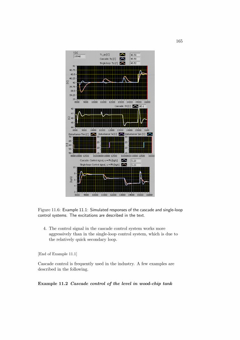
165

Figure 11.6: Example 11.1: Simulated responses of the cascade and single-loopcontrol systems. The excitations are described in the text.

4. The control signal in the cascade control system works moreaggressively than in the single-loop control system, which is due tothe relatively quick secondary loop.


Cascade control is frequently used in the industry. A few examples aredescribed in the following.

Example 11.2 Cascade control of the level in wood-chip tank

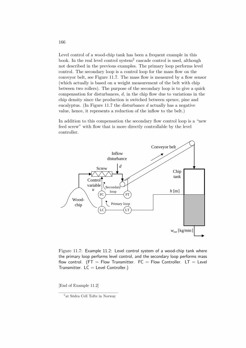
166

Level control of a wood-chip tank has been a frequent example in thisbook. In the real level control system2 cascade control is used, althoughnot described in the previous examples. The primary loop performs levelcontrol. The secondary loop is a control loop for the mass flow on theconveyor belt, see Figure 11.7. The mass flow is measured by a flow sensor(which actually is based on a weight measurement of the belt with chipbetween two rollers). The purpose of the secondary loop is to give a quickcompensation for disturbances, d, in the chip flow due to variations in thechip density since the production is switched between spruce, pine andeucalyptus. (In Figure 11.7 the disturbance d actually has a negativevalue, hence, it represents a reduction of the inflow to the belt.)

In addition to this compensation the secondary flow control loop is a “newfeed screw” with flow that is more directly controllable by the levelcontroller.

h [m]

Wood-chip

Chip tank

u

wout [kg/min]

LTLC

Controlvariable

FTFC

Primary loop

Secondaryloop

Conveyor belt

Screw d

Inflow disturbance

Figure 11.7: Example 11.2: Level control system of a wood-chip tank wherethe primary loop performs level control, and the secondary loop performs massflow control. (FT = Flow Transmitter. FC = Flow Controller. LT = LevelTransmitter. LC = Level Controller.)


2at Södra Cell Tofte in Norway

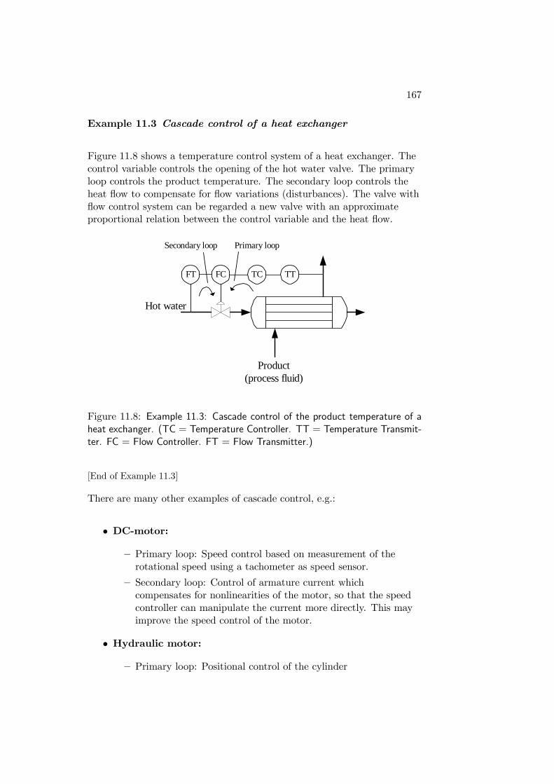
167

Example 11.3 Cascade control of a heat exchanger

Figure 11.8 shows a temperature control system of a heat exchanger. Thecontrol variable controls the opening of the hot water valve. The primaryloop controls the product temperature. The secondary loop controls theheat flow to compensate for flow variations (disturbances). The valve withflow control system can be regarded a new valve with an approximateproportional relation between the control variable and the heat flow.

FT TC TTFC

Product(process fluid)

Hot water

Secondary loop Primary loop

Figure 11.8: Example 11.3: Cascade control of the product temperature of aheat exchanger. (TC = Temperature Controller. TT = Temperature Transmit-ter. FC = Flow Controller. FT = Flow Transmitter.)


There are many other examples of cascade control, e.g.:

• DC-motor:

— Primary loop: Speed control based on measurement of therotational speed using a tachometer as speed sensor.

— Secondary loop: Control of armature current whichcompensates for nonlinearities of the motor, so that the speedcontroller can manipulate the current more directly. This mayimprove the speed control of the motor.

• Hydraulic motor:

— Primary loop: Positional control of the cylinder

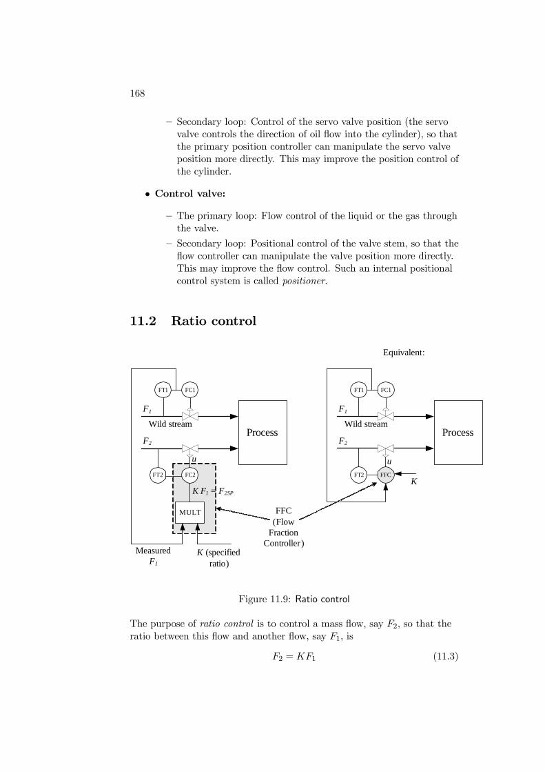
168

— Secondary loop: Control of the servo valve position (the servovalve controls the direction of oil flow into the cylinder), so thatthe primary position controller can manipulate the servo valveposition more directly. This may improve the position control ofthe cylinder.

• Control valve:

— The primary loop: Flow control of the liquid or the gas throughthe valve.

— Secondary loop: Positional control of the valve stem, so that theflow controller can manipulate the valve position more directly.This may improve the flow control. Such an internal positionalcontrol system is called positioner.

11.2 Ratio control

Process

FT1

FC2FT2

MULT

K (specifiedratio)

K F1 = F2SP

F1

MeasuredF1

F2

Wild stream

FC1

Process

FT1

FT2K

F1

F2

Wild stream

FC1

Equivalent:

FFC(Flow

Fraction Controller)

FFC

u u

Figure 11.9: Ratio control

The purpose of ratio control is to control a mass flow, say F2, so that theratio between this flow and another flow, say F1, is

F2 = KF1 (11.3)

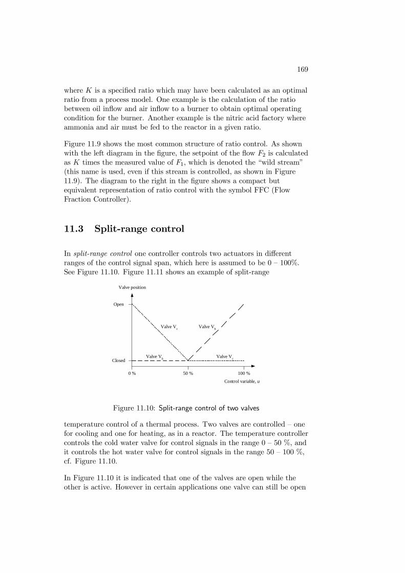
169

where K is a specified ratio which may have been calculated as an optimalratio from a process model. One example is the calculation of the ratiobetween oil inflow and air inflow to a burner to obtain optimal operatingcondition for the burner. Another example is the nitric acid factory whereammonia and air must be fed to the reactor in a given ratio.

Figure 11.9 shows the most common structure of ratio control. As shownwith the left diagram in the figure, the setpoint of the flow F2 is calculatedas K times the measured value of F1, which is denoted the “wild stream”(this name is used, even if this stream is controlled, as shown in Figure11.9). The diagram to the right in the figure shows a compact butequivalent representation of ratio control with the symbol FFC (FlowFraction Controller).

11.3 Split-range control

In split-range control one controller controls two actuators in differentranges of the control signal span, which here is assumed to be 0 — 100%.See Figure 11.10. Figure 11.11 shows an example of split-range

50 % 100 %0 %

Open

Control variable, u

Closed

Valve position

Valve Vc Valve Vh

Valve VcValve Vh

Figure 11.10: Split-range control of two valves

temperature control of a thermal process. Two valves are controlled — onefor cooling and one for heating, as in a reactor. The temperature controllercontrols the cold water valve for control signals in the range 0 — 50 %, andit controls the hot water valve for control signals in the range 50 — 100 %,cf. Figure 11.10.

In Figure 11.10 it is indicated that one of the valves are open while theother is active. However in certain applications one valve can still be open

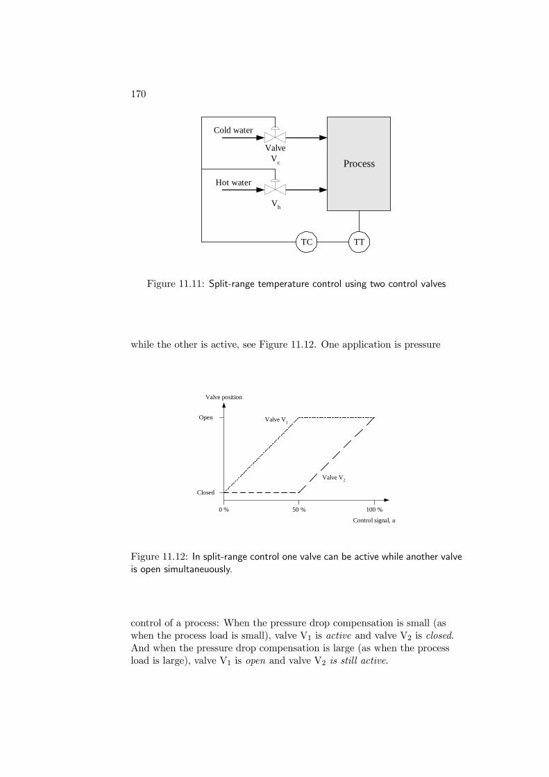
170

Process

TTTC

ValveVc

Vh

Cold water

Hot water

Figure 11.11: Split-range temperature control using two control valves

while the other is active, see Figure 11.12. One application is pressure

50 % 100 %0 %

Open

Control signal, u

Closed

Valve position

Valve V1

Valve V2

Figure 11.12: In split-range control one valve can be active while another valveis open simultaneuously.

control of a process: When the pressure drop compensation is small (aswhen the process load is small), valve V1 is active and valve V2 is closed.And when the pressure drop compensation is large (as when the processload is large), valve V1 is open and valve V2 is still active.

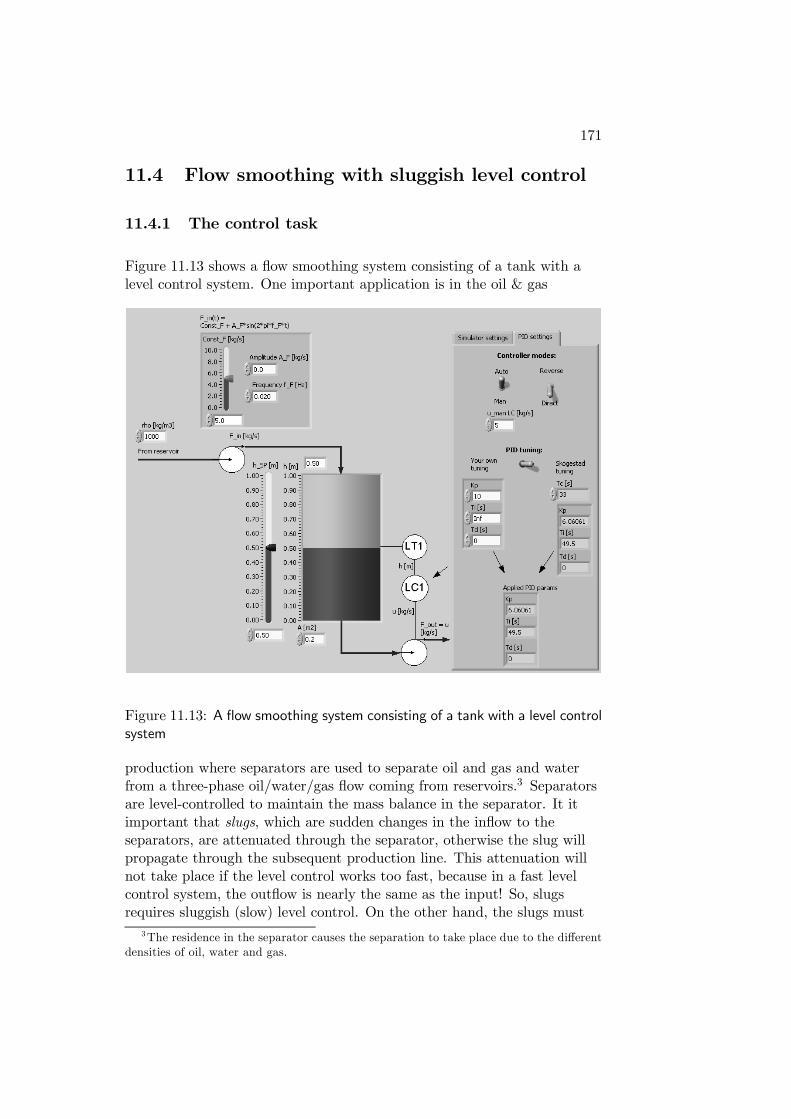
171

11.4 Flow smoothing with sluggish level control

11.4.1 The control task

Figure 11.13 shows a flow smoothing system consisting of a tank with alevel control system. One important application is in the oil & gas

Figure 11.13: A flow smoothing system consisting of a tank with a level controlsystem

production where separators are used to separate oil and gas and waterfrom a three-phase oil/water/gas flow coming from reservoirs.3 Separatorsare level-controlled to maintain the mass balance in the separator. It itimportant that slugs, which are sudden changes in the inflow to theseparators, are attenuated through the separator, otherwise the slug willpropagate through the subsequent production line. This attenuation willnot take place if the level control works too fast, because in a fast levelcontrol system, the outflow is nearly the same as the input! So, slugsrequires sluggish (slow) level control. On the other hand, the slugs must

3The residence in the separator causes the separation to take place due to the differentdensities of oil, water and gas.

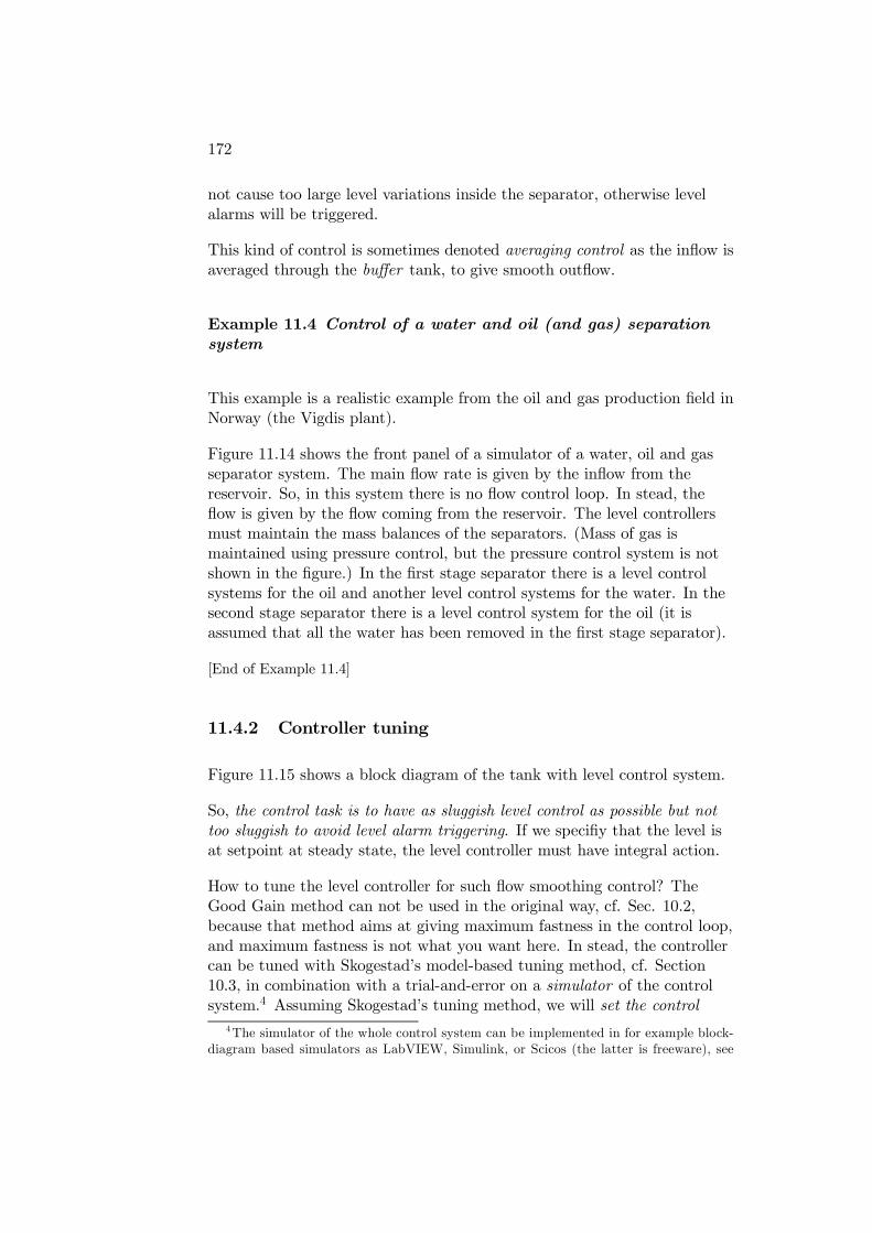
172

not cause too large level variations inside the separator, otherwise levelalarms will be triggered.

This kind of control is sometimes denoted averaging control as the inflow isaveraged through the buffer tank, to give smooth outflow.

Example 11.4 Control of a water and oil (and gas) separationsystem

This example is a realistic example from the oil and gas production field inNorway (the Vigdis plant).

Figure 11.14 shows the front panel of a simulator of a water, oil and gasseparator system. The main flow rate is given by the inflow from thereservoir. So, in this system there is no flow control loop. In stead, theflow is given by the flow coming from the reservoir. The level controllersmust maintain the mass balances of the separators. (Mass of gas ismaintained using pressure control, but the pressure control system is notshown in the figure.) In the first stage separator there is a level controlsystems for the oil and another level control systems for the water. In thesecond stage separator there is a level control system for the oil (it isassumed that all the water has been removed in the first stage separator).


11.4.2 Controller tuning

Figure 11.15 shows a block diagram of the tank with level control system.

So, the control task is to have as sluggish level control as possible but nottoo sluggish to avoid level alarm triggering. If we specifiy that the level isat setpoint at steady state, the level controller must have integral action.

How to tune the level controller for such flow smoothing control? TheGood Gain method can not be used in the original way, cf. Sec. 10.2,because that method aims at giving maximum fastness in the control loop,and maximum fastness is not what you want here. In stead, the controllercan be tuned with Skogestad’s model-based tuning method, cf. Section10.3, in combination with a trial-and-error on a simulator of the controlsystem.4 Assuming Skogestad’s tuning method, we will set the control

4The simulator of the whole control system can be implemented in for example block-diagram based simulators as LabVIEW, Simulink, or Scicos (the latter is freeware), see

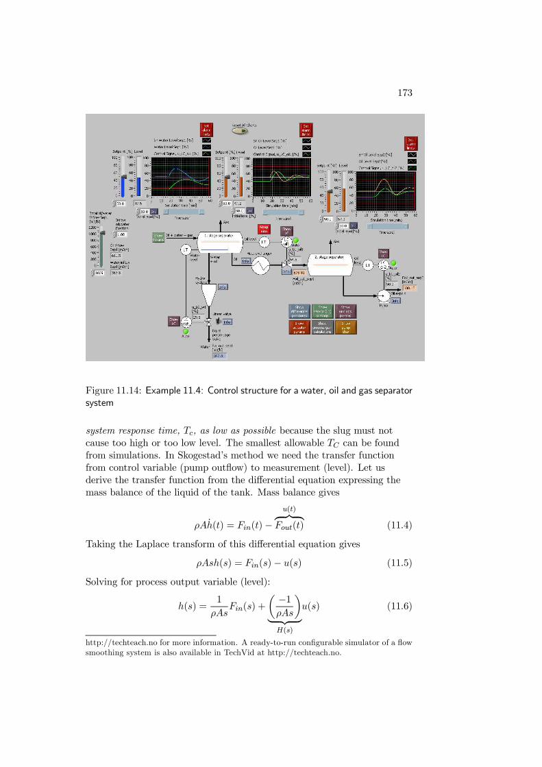
173

Figure 11.14: Example 11.4: Control structure for a water, oil and gas separatorsystem

system response time, Tc, as low as possible because the slug must notcause too high or too low level. The smallest allowable TC can be foundfrom simulations. In Skogestad’s method we need the transfer functionfrom control variable (pump outflow) to measurement (level). Let usderive the transfer function from the differential equation expressing themass balance of the liquid of the tank. Mass balance gives

ρAh(t) = Fin(t)−

u(t) Fout(t) (11.4)

Taking the Laplace transform of this differential equation gives

ρAsh(s) = Fin(s)− u(s) (11.5)

Solving for process output variable (level):

h(s) =1

ρAsFin(s) +

−1

ρAs

H(s)

u(s) (11.6)

http://techteach.no for more information. A ready-to-run configurable simulator of a flowsmoothing system is also available in TechVid at http://techteach.no.

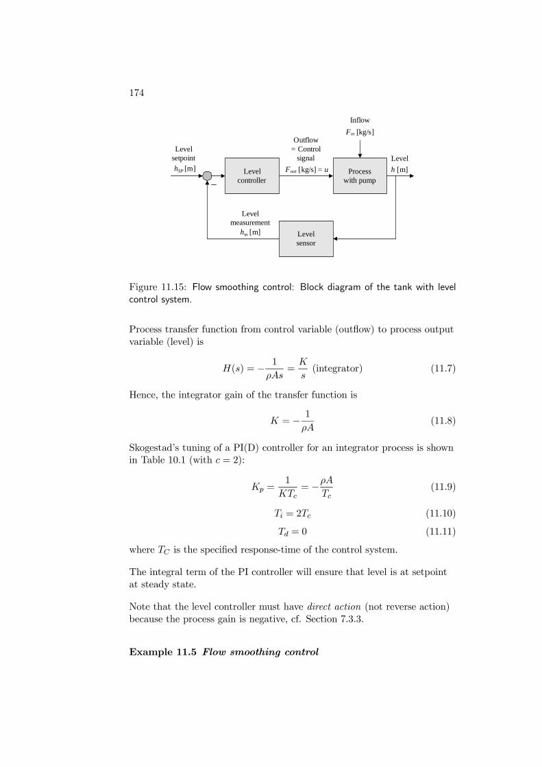
174

Processwith pump

Fin [kg/s]

h [m]hSP [m] Levelcontroller

Fout [kg/s] = u

Levelsensor

hm [m]

Level measurement

Levelsetpoint

Outflow = Control

signal Level

Inflow

Figure 11.15: Flow smoothing control: Block diagram of the tank with levelcontrol system.

Process transfer function from control variable (outflow) to process outputvariable (level) is

H(s) = −1

ρAs=

K

s(integrator) (11.7)

Hence, the integrator gain of the transfer function is

K = −1

ρA(11.8)

Skogestad’s tuning of a PI(D) controller for an integrator process is shownin Table 10.1 (with c = 2):

Kp =1

KTc= −

ρA

Tc(11.9)

Ti = 2Tc (11.10)

Td = 0 (11.11)

where TC is the specified response-time of the control system.

The integral term of the PI controller will ensure that level is at setpointat steady state.

Note that the level controller must have direct action (not reverse action)because the process gain is negative, cf. Section 7.3.3.

Example 11.5 Flow smoothing control

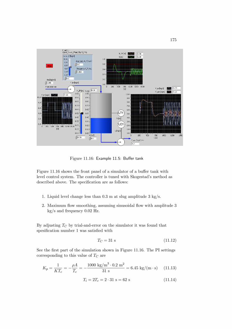
175

Figure 11.16: Example 11.5: Buffer tank

Figure 11.16 shows the front panel of a simulator of a buffer tank withlevel control system. The controller is tuned with Skogestad’s method asdescribed above. The specification are as follows:

1. Liquid level change less than 0.3 m at slug amplitude 3 kg/s.

2. Maximum flow smoothing, assuming sinusoidal flow with amplitude 3kg/s and frequency 0.02 Hz.

By adjusting TC by trial-and-error on the simulator it was found thatspesification number 1 was satisfied with

TC = 31 s (11.12)

See the first part of the simulation shown in Figure 11.16. The PI settingscorresponding to this value of TC are

Kp =1

KTc= −

ρA

Tc= −

1000 kg/m3 · 0.2 m2

31 s= 6.45 kg/(m · s) (11.13)

Ti = 2Tc = 2 · 31 s = 62 s (11.14)

176

Concerning specification number 2, the simulations show that thesinusoidal flow (amplitude 3 kg/s, frequency 0.02 Hz) has been attenuatedby a factor approximately equal to 25%. Hence, “flow gain” is 25%. If wetry to obtain even better flow smoothing by increasing TC further,specification number 1 will not be satisfied as the level response to thegiven slug will be larger than 0.3 m.


11.5 Plantwide control

In the process industry products are created after materials beingprocessed in a number of vessels in series, which are typically unitprocesses as evaporators, blending or heated tanks, buffer tanks, reactors,distillation columns, separators, absorbers, etc. Typical basic controlrequirements of such a production line are as follows:

• The product flow must be controlled (to follow a setpoint).This is typically done by implementing flow control of one keycomponent or feed.

• The product quality must be controlled — more or less directly.Ideally, the product quality is analyzed or measured in real time, andthis measurement is used to adjust feeds, supplied heat etc. so thatthe product quality is controlled to follow its setpoint using feedback.In practice, however, such real time or online measurements aretypically not implememented since they rely on time consuminglaboratory analysis. In stead, the product quality is controlledindirectly by controlling the flow of the feeds needed to produce thefinal product, typically using ratio control.

• The mass balance of each process vessel (tank, reactor, etc.)must be maintained — otherwise it may run full or empty. Themass balance is maintained with level control systems for liquids, andwith pressure control systems for gases. In vessels containing gasthere may still not be any pressure control. It depends on the processif it necessary to control the process.

It is crucial to select the correct reverse or direct action for each ofthe controllers (otherwise the control loop becomes unstable), cf.Section 7.3.3. The general rules are as follows5:

5 It is assumed that increased control signal to the actuator increases flow through theactuator.

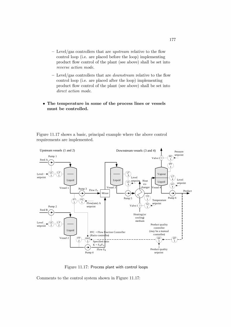
177

— Level/gas controllers that are upstream relative to the flowcontrol loop (i.e. are placed before the loop) implementingproduct flow control of the plant (see above) shall be set intoreverse action mode.

— Level/gas controllers that are downstream relative to the flowcontrol loop (i.e. are placed after the loop) implementingproduct flow control of the plant (see above) shall be set intodirect action mode.

• The temperature in some of the process lines or vesselsmust be controlled.

Figure 11.17 shows a basic, principal example where the above controlrequirements are implemented.

FT1 Flow(rate) A

setpoint

LT1

FC1

LC3 LC

4

LT4

Downstream vessels (3 and 4)Upstream vessels (1 and 2)

LC1

FFC1

FT2 Specified ratio

K = FB/FA

Pump 3

LT3

Vessel 1 Vessel 4

Pump 5 Pump 6

Levelsetpoint Level

setpoint Levelsetpoint

FFC = Flow Fraction Controller(Ratio controller)

LT2

LC2

Levelsetpoint

Pump 4

Vessel 3

Feed A

Feed B

ProductMixer

TC1

TT1 Temperature

setpoint

Heatex-

changer

PT1

PC1

Pressuresetpoint

Vessel 2

Heating (or cooling) medium

Vapour

Liquid

Valve 1

Valve 2

Liquid Liquid

Liquid

Pump 1

Pump 2

QT1

QC1

Product qualitysetpoint

Product qualitycontroller

(may be a manual controller)

Flow FA

Flow FB

Figure 11.17: Process plant with control loops

Comments to the control system shown in Figure 11.17:

178

• Two flows, FA and FB, are mixed. In general, the mix of two feedscan be fed to a subsequent reactor. It is assumed that FA containsthe key component of the product, and that FA defines theproduction rate. Ratio control is used to control FB so that the ratiobetween the flows is as specified:

K =FBFA

(11.15)

• The mass balance of upstream vessels 1 and 2 (upstream relative tothe point of production flow control in the process line) is controlledby manipulating inflows while the mass balance of the downstreamsvessels 3 and 4 tank are controlled by manipulating the outflows.

• In vessel 4 both the liquid level and the vapour pressure arecontrolled.

• The mass balances of liquids are maintained using level control. Themass balance of vapour is maintained using pressure control.

• The product quality may be controlled by adjusting the ratio Kbetween the flows into the mixer. Ideally, this quality controller isoperating in automatic mode based on online (continuous) qualitymeasurement of the product. However, in many cases (as in thenitric acid production plant described in Example 11.6) the productquality is measured off-line using laboratory analysis which givesquality measures only a few times per day. In these cases, the qualitycontroller is actually in the form of an operator adjusting the ratio K.

• The temperature of the inflow to vessel 4 is controlled.

• It is crucial to select correctly between Reverse action mode andDirect action mode in the controllers, cf. Section 7.3.3). Assume thatfor each of the pumps and the valves that increased control signalincrease pump speeds and increase valve openings. Furthermore,assume that heating is needed by the heat exchanger, the controlvalve manipulates the amount of heating medium. Then, thecontroller mode of each of the controllers are as follows:

— LC1: Reverse

— LC2: Reverse

— LC3: Direct

— LC4: Direct

— PC1: Reverse

— TC1: Reverse

179

— All flow controllers: Reverse

Is this correct?6

A specific, industrial example is given in the following.

Example 11.6 Control structures of a nitric acid plant

The example is about production of nitric acid, which is used in e.g. theproduction of fertilizers.7 The description of the process is based on [6],however I have simplified the process somewhat because too many detailsmay obscure the basic principles. (One simplification is that the bleacher,which is used to clean the raw, brown-coloured nitric acid which is theoutput from the asbsorber, is not included. Another simplification is thatthe condenser between compressor K2 and absorber A1 is not included.)The control structure is shown in the figure is based on information givenby Yara company in Porsgrunn, Norway.

Figure 11.18 shows a Process and Instrumentation Diagram (P & ID) ofthe (simplified) nitric acid plant.

Description of the nitric acid plant

(Control structures are described below.)

The feeds (input flows) to the production are

• Ammonia

• Air

• Process water

The product (output flow) is

• Nitric acid6No! PC1: Direct.7There are many Nitric Acid production plants around the world. One of them is at

the Yara industrial plant area in Porsgrunn, Norway.

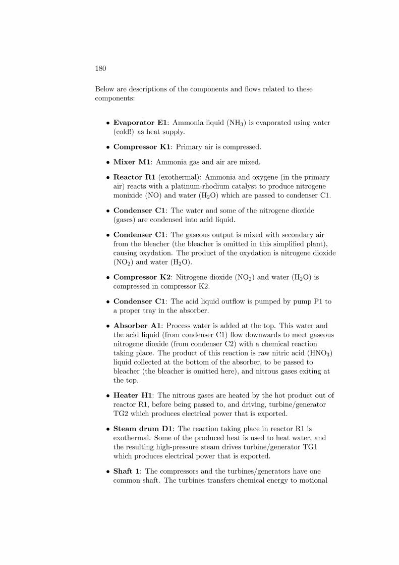
180

Below are descriptions of the components and flows related to thesecomponents:

• Evaporator E1: Ammonia liquid (NH3) is evaporated using water(cold!) as heat supply.

• Compressor K1: Primary air is compressed.

• Mixer M1: Ammonia gas and air are mixed.

• Reactor R1 (exothermal): Ammonia and oxygene (in the primaryair) reacts with a platinum-rhodium catalyst to produce nitrogenemonixide (NO) and water (H2O) which are passed to condenser C1.

• Condenser C1: The water and some of the nitrogene dioxide(gases) are condensed into acid liquid.

• Condenser C1: The gaseous output is mixed with secondary airfrom the bleacher (the bleacher is omitted in this simplified plant),causing oxydation. The product of the oxydation is nitrogene dioxide(NO2) and water (H2O).

• Compressor K2: Nitrogene dioxide (NO2) and water (H2O) iscompressed in compressor K2.

• Condenser C1: The acid liquid outflow is pumped by pump P1 toa proper tray in the absorber.

• Absorber A1: Process water is added at the top. This water andthe acid liquid (from condenser C1) flow downwards to meet gaseousnitrogene dioxide (from condenser C2) with a chemical reactiontaking place. The product of this reaction is raw nitric acid (HNO3)liquid collected at the bottom of the absorber, to be passed tobleacher (the bleacher is omitted here), and nitrous gases exiting atthe top.

• Heater H1: The nitrous gases are heated by the hot product out ofreactor R1, before being passed to, and driving, turbine/generatorTG2 which produces electrical power that is exported.

• Steam drum D1: The reaction taking place in reactor R1 isexothermal. Some of the produced heat is used to heat water, andthe resulting high-pressure steam drives turbine/generator TG1which produces electrical power that is exported.

• Shaft 1: The compressors and the turbines/generators have onecommon shaft. The turbines transfers chemical energy to motional

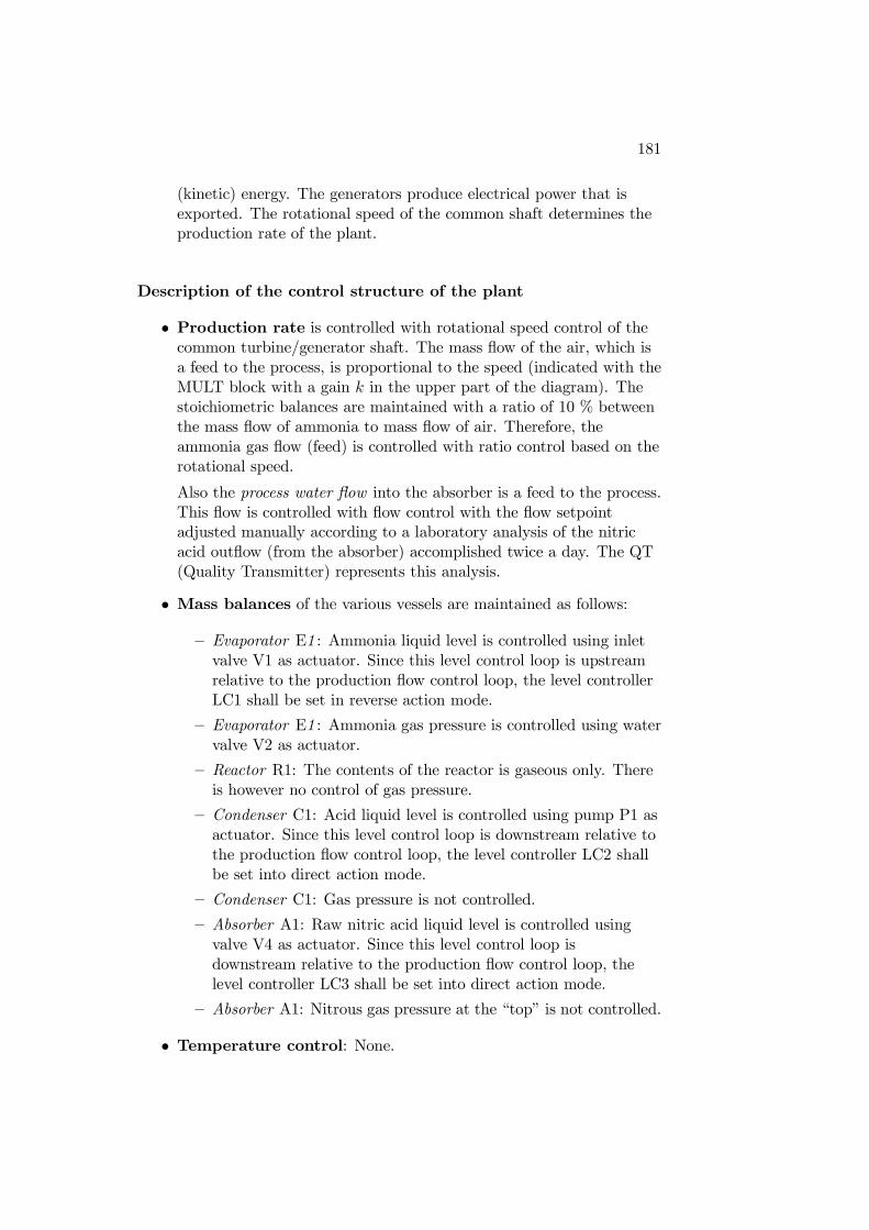
181

(kinetic) energy. The generators produce electrical power that isexported. The rotational speed of the common shaft determines theproduction rate of the plant.

Description of the control structure of the plant

• Production rate is controlled with rotational speed control of thecommon turbine/generator shaft. The mass flow of the air, which isa feed to the process, is proportional to the speed (indicated with theMULT block with a gain k in the upper part of the diagram). Thestoichiometric balances are maintained with a ratio of 10 % betweenthe mass flow of ammonia to mass flow of air. Therefore, theammonia gas flow (feed) is controlled with ratio control based on therotational speed.

Also the process water flow into the absorber is a feed to the process.This flow is controlled with flow control with the flow setpointadjusted manually according to a laboratory analysis of the nitricacid outflow (from the absorber) accomplished twice a day. The QT(Quality Transmitter) represents this analysis.

• Mass balances of the various vessels are maintained as follows:

— Evaporator E1 : Ammonia liquid level is controlled using inletvalve V1 as actuator. Since this level control loop is upstreamrelative to the production flow control loop, the level controllerLC1 shall be set in reverse action mode.

— Evaporator E1 : Ammonia gas pressure is controlled using watervalve V2 as actuator.

— Reactor R1: The contents of the reactor is gaseous only. Thereis however no control of gas pressure.

— Condenser C1: Acid liquid level is controlled using pump P1 asactuator. Since this level control loop is downstream relative tothe production flow control loop, the level controller LC2 shallbe set into direct action mode.

— Condenser C1: Gas pressure is not controlled.

— Absorber A1: Raw nitric acid liquid level is controlled usingvalve V4 as actuator. Since this level control loop isdownstream relative to the production flow control loop, thelevel controller LC3 shall be set into direct action mode.

— Absorber A1: Nitrous gas pressure at the “top” is not controlled.

• Temperature control: None.

182


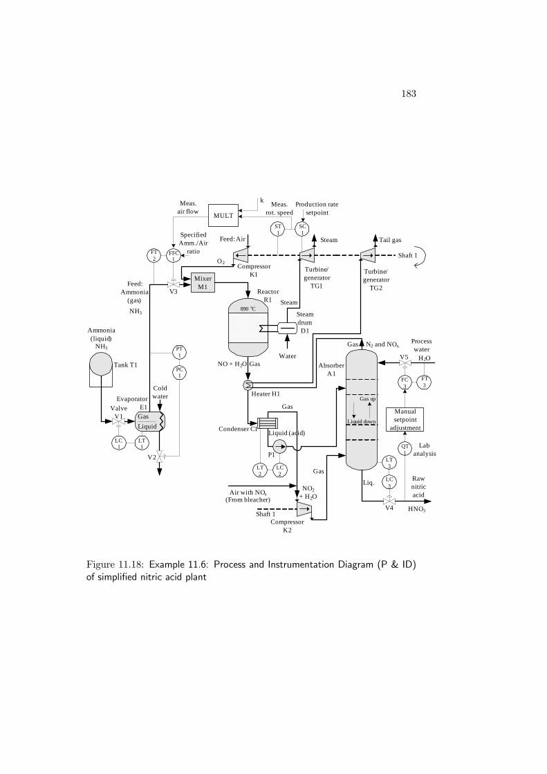
183

Tank T1

MixerM1

Process water

Reactor R1

Compressor K1

NH3

FT2

FFC1

LC1

LT1

PT1

PC1

Evaporator E1

Coldwater

Liquid

Gas

Ammonia(liquid)

LT2

LC2

Condenser C1

LT3

LC3

O2

890 oC

NO + H2O

Rawnitricacid

HNO3

H2OAbsorber

A1

N2 and NOx

Liquid (acid)

Gas

Shaft 1

Turbine/generator

TG2

Tail gas

Liquid down

Gas upHeater H1

Air with NOx

FC3

FT3

Feed:

Gas

V4

ValveV1

V2

V3

V5

P1

Manual setpoint

adjustment

QT1

NH3

Ammonia(gas)

Feed:

ST1

SC1

Air

Turbine/generator

TG1

Steam

Steam

Steam drumD1

Water

Gas

Gas

SpecifiedAmm./Air

ratio

Liq.

Lab analysis

Production ratesetpoint

Meas.rot. speedMULT

kMeas.air flow

(From bleacher)

NO2

+ H2O

Compressor K2

Shaft 1

Figure 11.18: Example 11.6: Process and Instrumentation Diagram (P & ID)of simplified nitric acid plant

Chapter 12

Sequential control

Sequential control is used to implement e.g. chemical batch process controland automated mechanical operations.

A sequential control procedure can be represented graphically by

• Sequential function chart (SFC), or

• State diagram.

SFCs have the following elements:

• Steps with a number of associated actions to be executed when thestep is active. A step is either active or passive. One particular stepis defined as the initial step. It can be symbolized with e.g. adouble-lined box, while ordinary steps are represented withsingle-lined boxes.

• Actions are control actions made by the control device (typically aPLC or a PC), e.g. opening a valve, setting a PID controller intoautomatic mode, starting a motor, lighting a lamp on, etc. Theaction box indicates the changes of control actions from previoussteps (control actions which are not changed, does not have to belisted in the action box).

• Transitions from one active step to another taking place when thetransition condition is satisfied. Transition conditions are in the formof logical expressions — simple or complicated — having value either

185

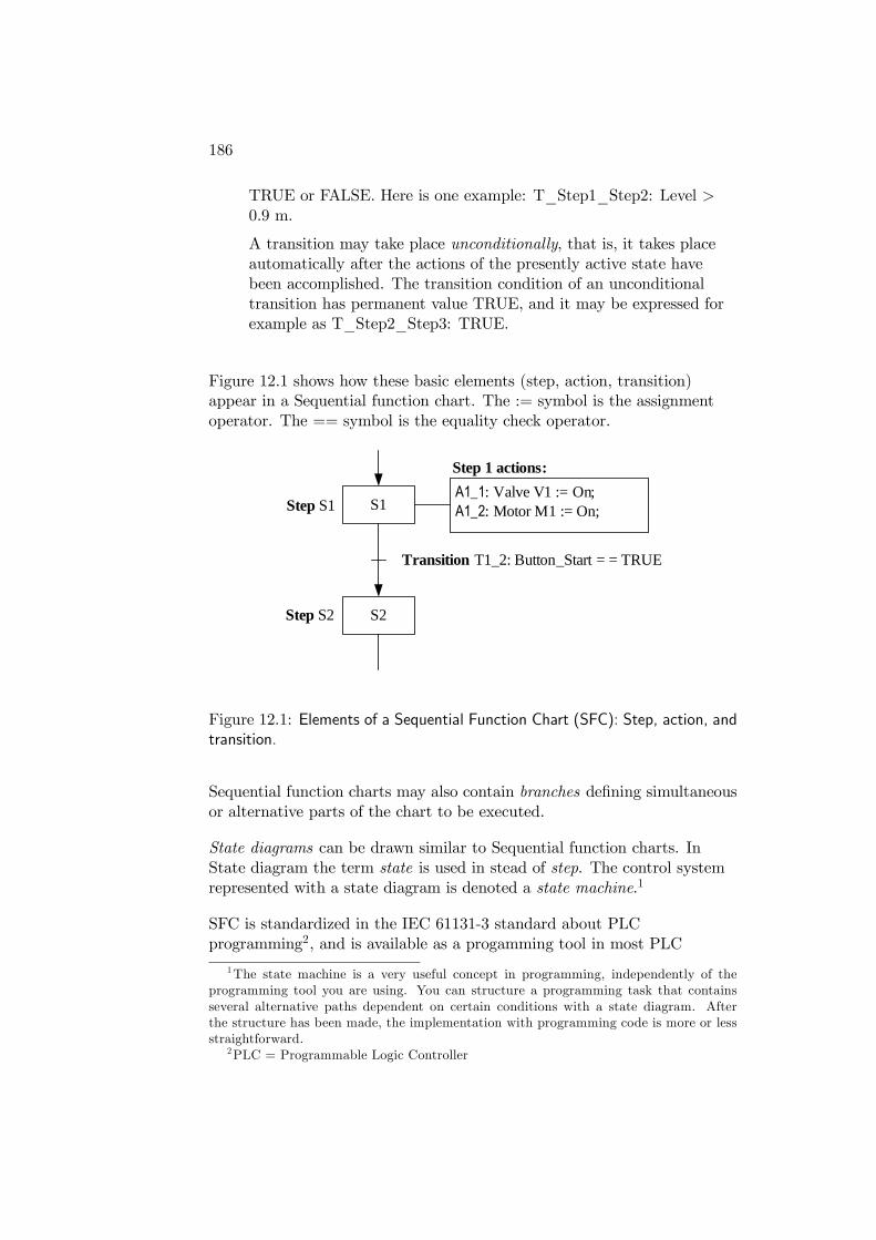
186

TRUE or FALSE. Here is one example: T_Step1_Step2: Level >0.9 m.

A transition may take place unconditionally, that is, it takes placeautomatically after the actions of the presently active state havebeen accomplished. The transition condition of an unconditionaltransition has permanent value TRUE, and it may be expressed forexample as T_Step2_Step3: TRUE.

Figure 12.1 shows how these basic elements (step, action, transition)appear in a Sequential function chart. The := symbol is the assignmentoperator. The == symbol is the equality check operator.

S1A1_1: Valve V1 := On;A1_2: Motor M1 := On;

Step 1 actions:

Step S1

S2Step S2

Transition T1_2: Button_Start = = TRUE

Figure 12.1: Elements of a Sequential Function Chart (SFC): Step, action, andtransition.

Sequential function charts may also contain branches defining simultaneousor alternative parts of the chart to be executed.

State diagrams can be drawn similar to Sequential function charts. InState diagram the term state is used in stead of step. The control systemrepresented with a state diagram is denoted a state machine.1

SFC is standardized in the IEC 61131-3 standard about PLCprogramming2, and is available as a progamming tool in most PLC

1The state machine is a very useful concept in programming, independently of theprogramming tool you are using. You can structure a programming task that containsseveral alternative paths dependent on certain conditions with a state diagram. Afterthe structure has been made, the implementation with programming code is more or lessstraightforward.

2PLC = Programmable Logic Controller

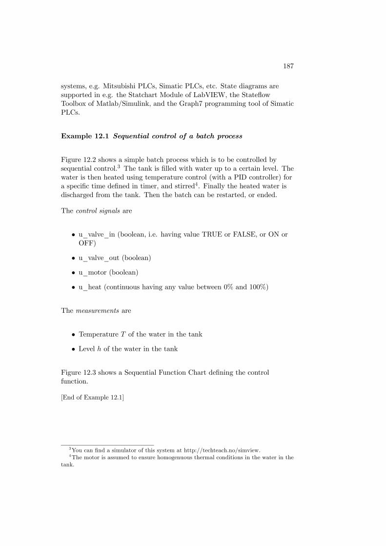
187

systems, e.g. Mitsubishi PLCs, Simatic PLCs, etc. State diagrams aresupported in e.g. the Statchart Module of LabVIEW, the StateflowToolbox of Matlab/Simulink, and the Graph7 programming tool of SimaticPLCs.

Example 12.1 Sequential control of a batch process

Figure 12.2 shows a simple batch process which is to be controlled bysequential control.3 The tank is filled with water up to a certain level. Thewater is then heated using temperature control (with a PID controller) fora specific time defined in timer, and stirred4. Finally the heated water isdischarged from the tank. Then the batch can be restarted, or ended.

The control signals are

• u_valve_in (boolean, i.e. having value TRUE or FALSE, or ON orOFF)

• u_valve_out (boolean)

• u_motor (boolean)

• u_heat (continuous having any value between 0% and 100%)

The measurements are

• Temperature T of the water in the tank

• Level h of the water in the tank

Figure 12.3 shows a Sequential Function Chart defining the controlfunction.


3You can find a simulator of this system at http://techteach.no/simview.4The motor is assumed to ensure homogenuous thermal conditions in the water in the

tank.

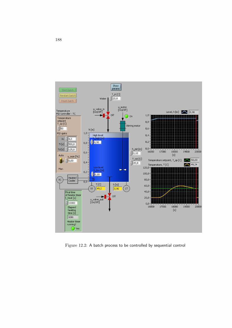
188

Figure 12.2: A batch process to be controlled by sequential control

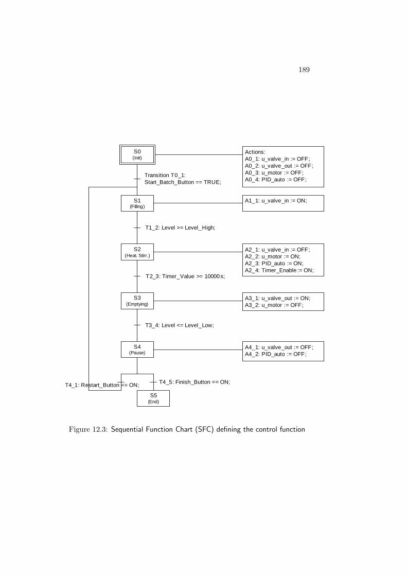
189

S0(Init)

Actions:A0_1: u_valve_in := OFF;A0_2: u_valve_out := OFF;A0_3: u_motor := OFF;A0_4: PID_auto := OFF;

S1(Filling)

Transition T0_1:Start_Batch_Button == TRUE;

A1_1: u_valve_in := ON;

T1_2: Level >= Level_High;

A2_1: u_valve_in := OFF;A2_2: u_motor := ON;A2_3: PID_auto := ON;A2_4: Timer_Enable := ON;

S2(Heat. Stirr.)

T2_3: Timer_Value >= 10000s;

S3(Emptying)

A3_1: u_valve_out := ON;A3_2: u_motor := OFF;

T3_4: Level <= Level_Low;

S4(Pause)

A4_1: u_valve_out := OFF;A4_2: PID_auto := OFF;

T4_5: Finish_Button == ON;

S5(End)

T4_1: Restart_Button == ON;

Figure 12.3: Sequential Function Chart (SFC) defining the control function

Appendix A

Codes and symbols used inProcess & InstrumentationDiagrams

This appendix gives a brief overview over codes and symbols used inProcess & Instrumentation Diagrams — P&IDs. The standards ISA S5.1(USA) and ISO 3511-1 (International) define the these diagrams. Thereare also factory internal standards.

A.1 Letter codes

Table A.1 shows the most commonly used letter codes used in Process &Instrumentation Diagrams.

A.2 Instrumentation symbols used in P&IDs

The following figures show common symbols used inProcess&Instrumentation Diagrams (P&IDs).

191

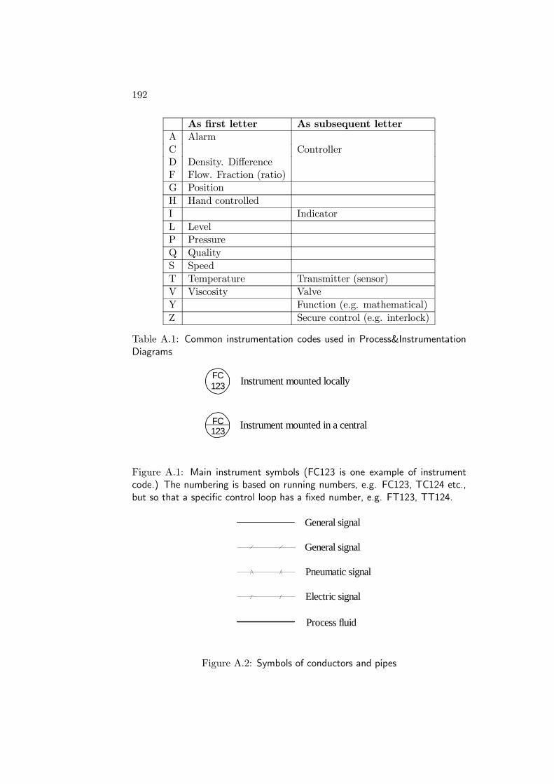
192

As first letter As subsequent letter

A AlarmC ControllerD Density. DifferenceF Flow. Fraction (ratio)G PositionH Hand controlledI IndicatorL LevelP PressureQ QualityS SpeedT Temperature Transmitter (sensor)V Viscosity ValveY Function (e.g. mathematical)Z Secure control (e.g. interlock)

Table A.1: Common instrumentation codes used in Process&InstrumentationDiagrams

Instrument mounted locally

Instrument mounted in a central

FC123

FC123

Figure A.1: Main instrument symbols (FC123 is one example of instrumentcode.) The numbering is based on running numbers, e.g. FC123, TC124 etc.,but so that a specific control loop has a fixed number, e.g. FT123, TT124.

General signal

Pneumatic signal

Electric signal

Process fluid

General signal

Figure A.2: Symbols of conductors and pipes

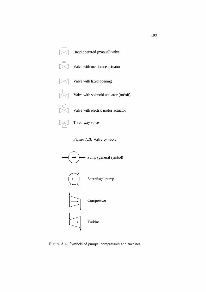
193

Hand operated (manual) valve

Valve with membrane actuator

Valve with fixed opening

Valve with solenoid actuator (on/off)

Valve with electric motor actuator

Three-way valve

Figure A.3: Valve symbols

Sentrifugal pump

Pump (general symbol)

Compressor

Turbine

Figure A.4: Symbols of pumps, compressors and turbines

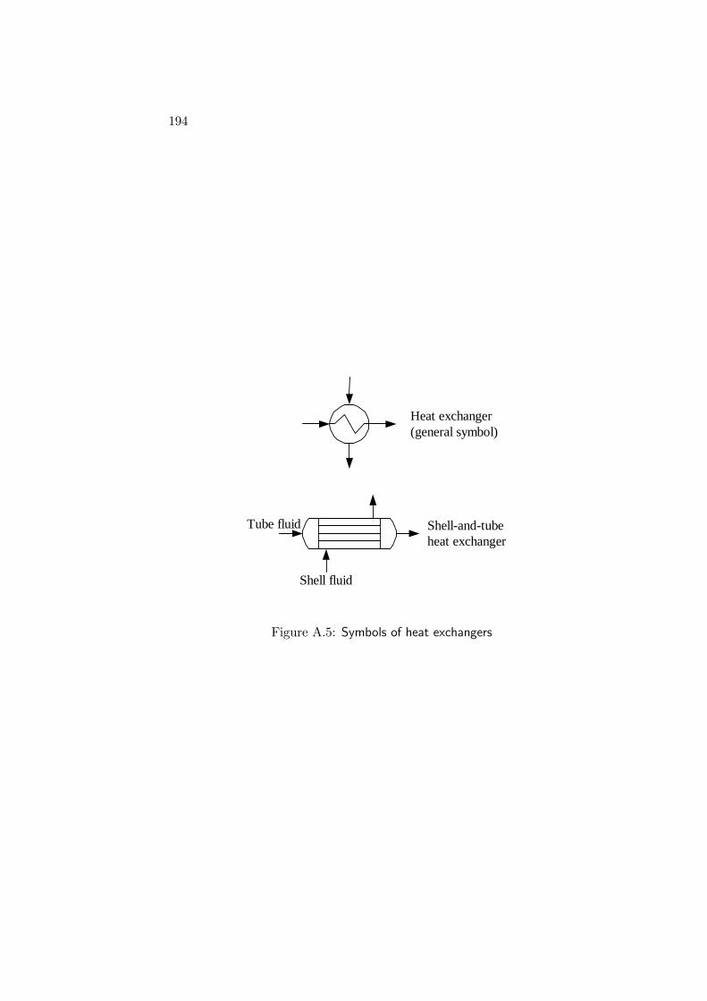
194

Heat exchanger(general symbol)

Shell-and-tubeheat exchanger

Tube fluid

Shell fluid

Figure A.5: Symbols of heat exchangers

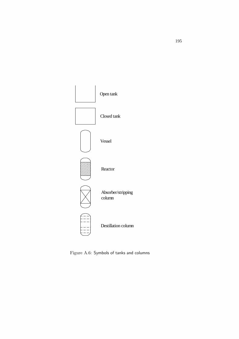
195

Open tank

Closed tank

Vessel

Reactor

Absorber/strippingcolumn

Destillation column

Figure A.6: Symbols of tanks and columns

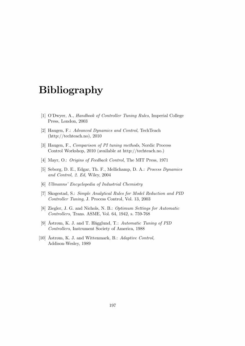
Bibliography

[1] O’Dwyer, A., Handbook of Controller Tuning Rules, Imperial CollegePress, London, 2003

[2] Haugen, F.: Advanced Dynamics and Control, TechTeach(http://techteach.no), 2010

[3] Haugen, F., Comparison of PI tuning methods, Nordic ProcessControl Workshop, 2010 (available at http://techteach.no.)

[4] Mayr, O.: Origins of Feedback Control, The MIT Press, 1971

[5] Seborg, D. E., Edgar, Th. F., Mellichamp, D. A.: Process Dynamicsand Control, 2. Ed, Wiley, 2004

[6] Ullmanns’ Encyclopedia of Industrial Chemistry

[7] Skogestad, S.: Simple Analytical Rules for Model Reduction and PIDController Tuning, J. Process Control, Vol. 13, 2003

[8] Ziegler, J. G. and Nichols, N. B.: Optimum Settings for AutomaticControllers, Trans. ASME, Vol. 64, 1942, s. 759-768

[9] Åstrøm, K. J. and T. Hägglund, T.: Automatic Tuning of PIDControllers, Instrument Society of America, 1988

[10] Åstrøm, K. J. and Wittenmark, B.: Adaptive Control,Addison-Wesley, 1989

197

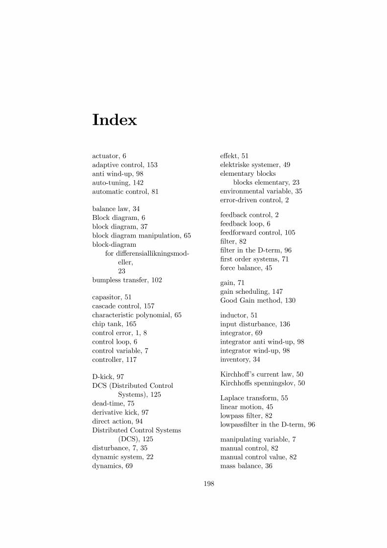
Index

actuator, 6adaptive control, 153anti wind-up, 98auto-tuning, 142automatic control, 81

balance law, 34Block diagram, 6block diagram, 37block diagram manipulation, 65block-diagram

for differensiallikningsmod-eller,23

bumpless transfer, 102

capasitor, 51cascade control, 157characteristic polynomial, 65chip tank, 165control error, 1, 8control loop, 6control variable, 7controller, 117

D-kick, 97DCS (Distributed Control

Systems), 125dead-time, 75derivative kick, 97direct action, 94Distributed Control Systems

(DCS), 125disturbance, 7, 35dynamic system, 22dynamics, 69

effekt, 51elektriske systemer, 49elementary blocks

blocks elementary, 23environmental variable, 35error-driven control, 2

feedback control, 2feedback loop, 6feedforward control, 105filter, 82filter in the D-term, 96first order systems, 71force balance, 45

gain, 71gain scheduling, 147Good Gain method, 130

inductor, 51input disturbance, 136integrator, 69integrator anti wind-up, 98integrator wind-up, 98inventory, 34

Kirchhoff’s current law, 50Kirchhoffs spenningslov, 50

Laplace transform, 55linear motion, 45lowpass filter, 82lowpassfilter in the D-term, 96

manipulating variable, 7manual control, 82manual control value, 82mass balance, 36

198

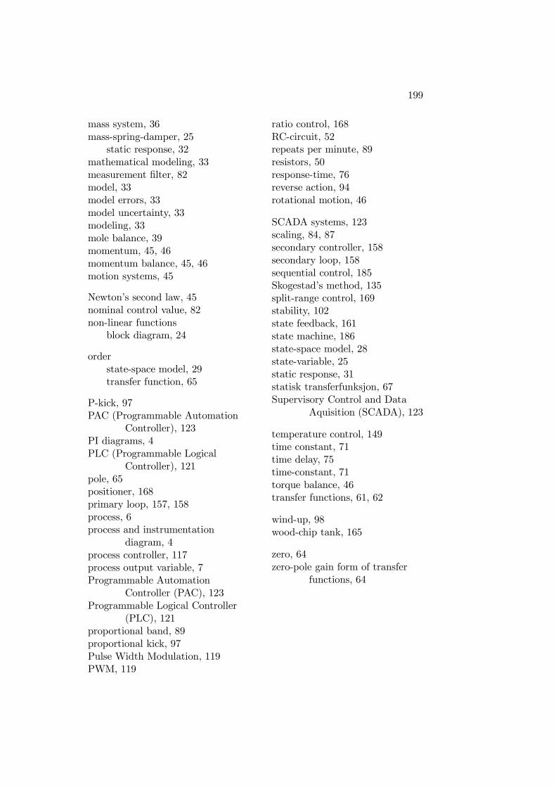
199

mass system, 36mass-spring-damper, 25

static response, 32mathematical modeling, 33measurement filter, 82model, 33model errors, 33model uncertainty, 33modeling, 33mole balance, 39momentum, 45, 46momentum balance, 45, 46motion systems, 45

Newton’s second law, 45nominal control value, 82non-linear functions

block diagram, 24

orderstate-space model, 29transfer function, 65

P-kick, 97PAC (Programmable Automation

Controller), 123PI diagrams, 4PLC (Programmable Logical

Controller), 121pole, 65positioner, 168primary loop, 157, 158process, 6process and instrumentation

diagram, 4process controller, 117process output variable, 7Programmable Automation

Controller (PAC), 123Programmable Logical Controller

(PLC), 121proportional band, 89proportional kick, 97Pulse Width Modulation, 119PWM, 119

ratio control, 168RC-circuit, 52repeats per minute, 89resistors, 50response-time, 76reverse action, 94rotational motion, 46

SCADA systems, 123scaling, 84, 87secondary controller, 158secondary loop, 158sequential control, 185Skogestad’s method, 135split-range control, 169stability, 102state feedback, 161state machine, 186state-space model, 28state-variable, 25static response, 31statisk transferfunksjon, 67Supervisory Control and Data

Aquisition (SCADA), 123

temperature control, 149time constant, 71time delay, 75time-constant, 71torque balance, 46transfer functions, 61, 62

wind-up, 98wood-chip tank, 165

zero, 64zero-pole gain form of transfer

functions, 64

Ojo Libro Dynamica

Documents

Transcript of Ojo Libro Dynamica