
Modelling of a Variable Venturi in a Heavy Duty Diesel Engine
70
Modelling of a Variable Venturi in a Heavy Duty Diesel Engine Master’s thesis performed in Vehicular Systems by Carl-AdamTorbj¨ornsson Reg nr: LiTH-ISY-EX-3368-2002 18th December 2002
Transcript of Modelling of a Variable Venturi in a Heavy Duty Diesel Engine

Modelling of a Variable Venturi in aHeavy Duty Diesel Engine
Master’s thesisperformed in Vehicular Systems
byCarl-Adam Torbjornsson
Reg nr: LiTH-ISY-EX-3368-2002
18th December 2002


Modelling of a Variable Venturi in aHeavy Duty Diesel Engine
Master’s thesis
performed in Vehicular Systems,Dept. of Electrical Engineering
at Linkopings universitet
by Carl-Adam Torbjornsson
Reg nr: LiTH-ISY-EX-3368-2002
Supervisor: Mattias Nyberg, PhDSCANIA CV
Jonas Biteus, MScLinkopings Universitet
Examiner: Professor Lars NielsenLinkopings Universitet
Linkoping, 18th December 2002


Avdelning, InstitutionDivision, Department
DatumDate
Sprak
Language
� Svenska/Swedish
� Engelska/English
�
RapporttypReport category
� Licentiatavhandling
� Examensarbete
� C-uppsats
� D-uppsats
� Ovrig rapport
�URL for elektronisk version
ISBN
ISRN
Serietitel och serienummerTitle of series, numbering
ISSN
Titel
Title
ForfattareAuthor
SammanfattningAbstract
NyckelordKeywords
The objectives in this thesis are to present a model of a variable ven-turi in an exhaust gas recirculation (EGR) system located in a heavyduty diesel engine. A new legislation called EURO 4 will come intoforce in 2005 which affects truck development and it will require anOn-Board Diagnostic system in the truck. If model based diagnosticsystems are to be used, one of the advantages is that the system per-formance will increase if a model of a variable venturi is used.
Three models with different complexity are compared in ten differentexperiments. The experiments are performed in a steady flow rig atdifferent percentage of EGR gases and venturi areas. The model pre-dicts the mass flow through the venturi. The results show that the firstmodel with fewer simplifications performs better and has fewer errorsthan the other two models. The simplifications that differ between themodels are initial velocity before the venturi and the assumption ofincompressible flow.
The model that shows the best result is not proposed by known lit-erature in this area of knowledge and technology. This thesis showsthat further studies and work on this model, the model with fewersimplifications, can be advantageous.
Vehicular Systems,Dept. of Electrical Engineering581 83 Linkoping
18th December 2002
—
LITH-ISY-EX-3368-2002
—
http://www.vehicular.isy.liu.sehttp://www.ep.liu.se/exjobb/isy/2002/3368/
Modelling of a Variable Venturi in a Heavy Duty Diesel Engine
Modellering av variabel venturi i en dieselmotor for tung lastbil
Carl-Adam Torbjornsson
××
Exhaust gas recirculation, On-board Diagnostic, Flow meter, ModelBased Diagnostic, Restriction, Compressible, Incompressible


Abstract
The objectives in this thesis are to present a model of a variable venturiin an exhaust gas recirculation (EGR) system located in a heavy dutydiesel engine. A new legislation called EURO 4 will come into force in2005 which affects truck development and it will require an On-BoardDiagnostic system in the truck. If model based diagnostic systems areto be used, one of the advantages is that the system performance willincrease if a model of a variable venturi is used.
Three models with different complexity are compared in ten differ-ent experiments. The experiments are performed in a steady flow rigat different percentage of EGR gases and venturi areas. The modelpredicts the mass flow through the venturi. The results show that thefirst model with fewer simplifications performs better and has fewer er-rors than the other two models. The simplifications that differ betweenthe models are initial velocity before the venturi and the assumptionof incompressible flow.
The model that shows the best result is not proposed by knownliterature in this area of knowledge and technology. This thesis showsthat further studies and work on this model, the model with fewersimplifications, can be advantageous.
Keywords: Exhaust gas recirculation, On-board Diagnostic, Flowmeter, Model Based Diagnostic, Restriction, Compressible, In-compressible
v

Acknowledgment
This thesis has been done on a commission from Scania CV, Sodertalje.I would like to thanks the people at the department of Software andDiagnostics, Engine Control Systems who made my stay very pleas-ant. Special thanks go to Mattias Nyberg, Olof Lundstrom and MikaelAndersson at NMCS and Henrik Hoglund and Jorgen Mardberg atNMEE which help I could not have been without. At Vehicular Sys-tems, Linkopings universitet a special thanks goes to my examinatorLars Nielsen and my supervisor Jonas Biteus.
Linkoping, December 2002Carl-Adam Torbjornsson
vi

Contents
Abstract v
Preface and Acknowledgment vi
1 Introduction 11.1 Background . . . . . . . . . . . . . . . . . . . . . . . . . 1
1.1.1 EURO 4 . . . . . . . . . . . . . . . . . . . . . . . 11.1.2 Heavy duty diesel engine . . . . . . . . . . . . . 21.1.3 Exhaust gas recirculation engine . . . . . . . . . 3
1.2 Objectives . . . . . . . . . . . . . . . . . . . . . . . . . . 31.3 Target group . . . . . . . . . . . . . . . . . . . . . . . . 41.4 Delimitation . . . . . . . . . . . . . . . . . . . . . . . . . 51.5 Methods . . . . . . . . . . . . . . . . . . . . . . . . . . . 51.6 Methods criticism . . . . . . . . . . . . . . . . . . . . . . 51.7 Reader’s guide . . . . . . . . . . . . . . . . . . . . . . . 5
2 Exhaust gas recirculation models 62.1 Venturi . . . . . . . . . . . . . . . . . . . . . . . . . . . 7
2.1.1 Variable venturi . . . . . . . . . . . . . . . . . . 82.2 General equations . . . . . . . . . . . . . . . . . . . . . 92.3 Venturi model 1 . . . . . . . . . . . . . . . . . . . . . . . 112.4 Venturi model 2 . . . . . . . . . . . . . . . . . . . . . . . 132.5 Venturi model 3 . . . . . . . . . . . . . . . . . . . . . . . 13
3 Experiment 153.1 Percent exhaust gas recirculation . . . . . . . . . . . . . 153.2 Collecting data . . . . . . . . . . . . . . . . . . . . . . . 20
3.2.1 Pressure and temperature sensor . . . . . . . . . 203.2.2 Mass flow sensor . . . . . . . . . . . . . . . . . . 21
3.3 Translate data . . . . . . . . . . . . . . . . . . . . . . . 223.4 Air velocity . . . . . . . . . . . . . . . . . . . . . . . . . 22
vii

4 Results 244.1 Model fitting . . . . . . . . . . . . . . . . . . . . . . . . 24
4.1.1 Venturi model 1 . . . . . . . . . . . . . . . . . . 264.1.2 Venturi model 2 . . . . . . . . . . . . . . . . . . 264.1.3 Venturi model 3 . . . . . . . . . . . . . . . . . . 27
4.2 Residual results . . . . . . . . . . . . . . . . . . . . . . . 284.3 Air velocity . . . . . . . . . . . . . . . . . . . . . . . . . 314.4 Discussion . . . . . . . . . . . . . . . . . . . . . . . . . . 31
4.4.1 Venturi model 1 . . . . . . . . . . . . . . . . . . 324.4.2 Venturi model 2 . . . . . . . . . . . . . . . . . . 334.4.3 Venturi model 3 . . . . . . . . . . . . . . . . . . 334.4.4 Residual results . . . . . . . . . . . . . . . . . . . 334.4.5 Discharge coefficient . . . . . . . . . . . . . . . . 34
5 Conclusions and extensions 355.1 Conclusions . . . . . . . . . . . . . . . . . . . . . . . . . 355.2 Extensions . . . . . . . . . . . . . . . . . . . . . . . . . . 36
References 37
Notation 39
A Equations 40A.1 General equations . . . . . . . . . . . . . . . . . . . . . 40A.2 Derivations . . . . . . . . . . . . . . . . . . . . . . . . . 40
B Results 42B.1 Velocities through the venturi . . . . . . . . . . . . . . 42B.2 Venturi model 1 . . . . . . . . . . . . . . . . . . . . . . . 45B.3 Venturi model 2 . . . . . . . . . . . . . . . . . . . . . . . 50B.4 Venturi model 3 . . . . . . . . . . . . . . . . . . . . . . . 55
viii

Chapter 1
Introduction
This thesis attempts to solve the problem of modelling the mass flowof an Exhaust Gas Recirculation (EGR) system. The problem is solvedon a commission from Scania CV and within the final project and mas-ter’s thesis made at Scania Sodertalje, and at the division of VehicularSystems at Linkopings universitet. In this chapter the objective, spec-ification and background of this master’s thesis are discussed.
1.1 Background
Scania was founded in 1891 and is today one of the world’s leadingmanufacturers of heavy trucks and buses. Scania is an internationalcorporation with operations in more than 100 countries. Ninety-sevenpercent of its production is sold outside Sweden. [1]
The trucks are developed, manufactured and sold with diesel en-gines due to the enhanced efficiency of a diesel engine compared to, forexample, a petrol engine. Although the emissions today are higher witha diesel engine than other engines, there are several ways of reducingthe diesel engine emissions.
1.1.1 EURO 4
In October 2005 a new legislation called EURO 4 will come into forcethat affects truck development. This will include limits for exhaustgas emission on Heavy Duty Diesel (HDD) vehicles. The legislator inEurope is the European Union and in the USA, the EnvironmentalProtection Agency (EPA). The EU sets limits in Europe with EUROlegislations.
EURO 4 limits for oxides of nitrogen (NOx) is 3.5 g/kWh andfor PM (particulate matter) it is 0.02 g/kWh, compared to EURO 3
1

2 Introduction
limits of 5.0 g/kWh for NOx and 0.1 g/kWh of PM emissions. Thenext legislation, EURO 5 will have even tougher specification limits.However, these limits have not yet been determined. EURO 4 will alsorequire an On-Board Diagnostic (OBD) system. When there is a riskthat an error on the truck will lead to increased emission, the driver willbe warned by the system. One way of alerting the driver is a warninglight on the dashboard.
A possible way of creating this OBD system is through Model BasedDiagnostic. By using a model of the engine parallel with the enginesharing the same input1 and output2 signals. When the model of theengine and the real engine differ and there is a risk of increased emission,the driver will be notified. The incident will also be recorded in alogging device of the engine.
1.1.2 Heavy duty diesel engine
A diesel engine and a petrol engine differs more than just the fuel usedto run the engine. Most cars today run with a four stroke spark ignitedpetrol engine. Heavy trucks runs on diesel engines mostly due to theirhigher efficiency. The main differences between the petrol engine andthe diesel engine are:
Ignition A petrol engine intakes a mixture of gas and air, compressesit and ignites the mixture with a spark. A diesel engine takes injust air, compresses it and then injects fuel into the compressedair. The heat of the compressed air lights the fuel spontaneously.
Pressurization A petrol engine compresses at a ratio of 8:1 to 12:1,while a diesel engine compresses at a ratio of 14:1 to as high as25:1. The higher compression ratio of the diesel engine the betterefficiency.
Feeding of fuel A petrol engine generally uses either carburetion, inwhich the air and fuel is mixed long before the air enters thecylinder, or port fuel injection, in which the fuel is injected justprior to the intake stroke (outside the cylinder). Diesel enginesuse direct fuel injection, the diesel fuel is injected directly intothe cylinder.
Another difference between diesel engines and petrol engines is inthe injection process. Most car engines use port injection or a carbu-retor rather than direct injection. Therefore, in a car engine, all of
1Examples of input signals are: Throttle, intake air temperature, engine tem-perature, amount air flowing into the engine and signal from lambda sensor.
2Examples of output signals are: Engines torque, emissions such as NOx andPM, fuel consumption and voltage from the generator.
1.2. Objectives 3
the fuel is loaded into the cylinder during the intake stroke and thencompressed. The compression of the mixture of gas and air limits thecompression ratio of the engine. If it compresses the air too much,the mixture of gas and air spontaneously ignites and causes knocking.A diesel compresses only air, so the compression ratio can be muchhigher. The higher the compression ratio, the more power is generated.Therefore the higher efficiency. [2]
1.1.3 Exhaust gas recirculation engine
Oxygen is required for fuel to burn in an engine. This is usually suppliedby taking in air from the atmosphere. The high temperatures foundwithin the engine cause nitrogen to react with oxygen to form NOx.
The burned gases act as a diluent in the unburned mixture;the absolute temperature reached after combustion variesinversely with the burned gas mass fraction. Hence increas-ing the burned gas fraction reduces NO emissions levels.
Addition of diluents [exhaust gas (EGR) and nitrogen] re-duce peak flame temperatures and NOx emissions; also,addition of oxygen (which corresponds to a reduction indiluent fraction) increase flame temperatures and thereforeincrease NOx emissions.
Diluents added to the intake air (such as recycled exhaust)are effective at reducing the NO formation rate, and there-fore NOx exhaust emissions. [3]
NOx are one of the main pollutants emitted by vehicle engines and arelegislated by EURO 4. One way to control NOx is to use EGR. Thistechnique directs some of the exhaust gases back into the intake of theengine to dilute the fresh air.
There is one small problem with EGR though. In a worst casescenario, at low engine load and speed, the pressure difference betweenthe exhaust and the inlet of the engine could level out, or even worse,could lead to a negative pressure drop and the EGR gases would notflow towards the inlet manifold. Figure 1.1 identifies the name of thedifferent pressures and the alignment of an EGR system on a HDDengine. To move low pressured gas to a high pressured chamber withoutloosing too much efficiency is difficult. How this problem affects theEGR and is solved is explained in Chapter 2.
1.2 Objectives
In order to satisfy EURO 4, an OBD system is needed and lower NOx
emissions are required. An EGR-system lowers NOx emissions, and if

4 Introduction
�������
���� ��
��� ��
��������
��
�������
�����������
����
���
���
���
����
Figure 1.1: Sketch of a turbo charged engine with EGR.
EGR is used the EGR must be diagnosed and modelled.
The venturi is one way of making the EGR work. To make the EGRmodel function, and to be able to diagnose the venturi, the venturishould be modelled.
The objectives of this thesis are to present a model of a variableventuri that can be used to model the mass flow through the EGR.Thereafter, verify how the same model models the mass flow throughthe whole variable venturi.
1.3 Target group
The target groups of this thesis are the people working at Scania CV,undergraduate students, graduate students and others at the divisionof Vehicular Systems at Linkopings universitet. Even others that havesome knowledge and interest of fluid dynamics, diagnosis and enginesmay have interest of this.
To fully understand the theory and results presented, common knowl-edge of diesel and petrol engines, fluid dynamics, control theory anddiagnosis are required.

1.4. Delimitation 5
1.4 Delimitation
Data needed to solve the problem are collected when needed from ex-periments performed with existing equipment. Only one venturi is usedduring measurements.
1.5 Methods
The methods are based on literature studies and experiments.To find literature that makes enough assumptions to help solve the
problem in this case, before the results are available and evaluated, isdifficult and therefore iterative problem solving is used. Recommenda-tions made by the authors and other specialists in this subject area areconsidered. Experiments are of qualitative characteristic and based onobservations and data collecting sessions with available equipment.
1.6 Methods criticism
One problem with fluid dynamics is that there is no exact analytic so-lution without any assumptions made, it is simply too complicated. [4]That said, the task is to solve the problem with enough assumptions,so the problem can be solved in an analytical way without becomeinginaccurate.
Books were used to collect theory, which mainly is used in educa-tion at undergraduate courses. The books used were recommended byprofessors and experts and is a small part of the existing literature.
The use of not optimal experiment equipment, not calibrated sen-sors or a controlled environment where the experiments took place canworsen the model and the results. Temperature, pressure and massflow of air or mass flow of EGR gases could not reach real values as ina real running engine.
1.7 Reader’s guide
Chapters follow a logical order of designing a model of an EGR, in achronological order. Create the model with equations first, Chapter 2,to be able to pick which variable to measure. Then, measure and collectdata of different parts of the EGR system, Chapter 3. Verify the modelwith experiments data, Chapter 4 and analyze the result. Finally adiscussion, Section 4.4 before Chapter 5 rounds up this thesis with aconclusion and extension.

Chapter 2
Exhaust gasrecirculation models
This chapter includes the theory of exhaust gas recirculation and moreprecise the theory of the variable venturi. It also includes how EGRfunction, where EGR is introduced on an engine and how to model thecritical part of the EGR, the variable venturi.
As explained in Section 1.1.2 there is a problem with EGR systems.The problem is not the system itself but the characteristic of the engineit is mounted upon. If EGR system is introduced on an engine there areseveral things and parts which must be considered. The most evidentcharacteristic of a turbo charged HDD engine is the magnitude of itsdifferent pressures through out the engine. For an example, after theturbo has compressed the air and the intercooler has cooled down theair and lowered the pressure the air still has about 3 bar mean valueof pressure at full load. To reach highest possible efficiency all of thepressure from the combustion should be used to accelerate the piston.That means the pressure should be near ambient pressure, about 1 bar,when leaving the combustion chamber to the exhaust manifold. How-ever, in reality the pressure is still high and the rest of the gas energyis used to spin the turbine so the compressor can compress the air atthe intake side of the engine.
The main task for EGR system is, as told before, to lower NOx
emissions. Therefore, the EGR has to somehow move an amount of theburned gas from the low pressure in the exhaust manifold to the highpressure inlet manifold. But as gas flows from high pressure to lowpressure if no work is done on the gas. As there is a much higher meanvalue pressure in the inlet manifold then in the exhaust manifold thenet flow would be flowing the wrong way, from the inlet manifold tothe exhaust manifold and that would lower the efficiency of the engine.
6

2.1. Venturi 7
The engine might even stop working properly.There are two possibilities to make EGR function. Either work on
the gas, for an example a compressor or some kind of a pump would dothe work on the gas to raise the gas pressure. If the pressure is raisedthen the gas could flow towards the inlet manifold. Secondly lower thepressure on the air in the inlet manifold to allow the burned gases fromthe exhaust manifold flow towards a lower pressure. As always all lossesmust be reduced. The first idea of work on the gas would further makethe system more complex and therefore the first possibility is rejected.
To maintain a positive flow of gases from exhaust manifold to inletmanifold the pressure difference PEM − PIM in Figure 1.1 must bepositive. There are two common ways of doing this:
1. Introduce a throttle between the intercooler and the intake. Witha throttle it is easy to control the pressure difference PEM −PIM
but with a huge impact on the efficiency due to the low pressureof air before combustion.
2. Use a venturi pipe between the intercooler and the inlet manifold.Due to the venturi’s characteristic there will be a local lowering ofthe pressure at the venturi throat. Where the pressure is loweredthe EGR gases should be lead into the venturi.
As explained earlier, higher pressure of air before combustion leadsto higher efficiency which means a lowering of the pressure is out of thequestion. The venturi pipe would only lower the pressure at a smallsection to allow the EGR gas to dilute the fresh air before the inlet andtherefore is the better choice.
2.1 Venturi
The main difference between a throttle and a venturi is that the ven-turi has a diffusor after the venturi throat. This does not change theequation used as will be shown. However, this is easy realized whenthe same equations is used to derive the throttle, the venturi and thenozzle. The main differences between the equations of a throttle and aventuri are constants which depends on geometry. The nozzle is calcu-lated as a restriction. The diffusors main task is to raise the pressureto what it was before the restriction.
In Figure 2.1 the intersection ∗ can be placed anywhere betweensection 0 and ∗ but is placed at the venturi throat where the area issmallest.
If the venturi is to be seen as two parts, from left to right in Fig-ure 2.1, one converging part called a restriction or nozzle and one di-verging part called a diffusor. The two parts connects at the narrow

8 Chapter 2. Exhaust gas recirculation models
���
Figure 2.1: Split view of a schematic venturi. The intersection of index∗ is placed at an arbitrary position between indexes 0 and 2.
part, a throat called section ∗. This passage is often called a criticalpassage due to the possibility to accelerate air to super sonic speedswhen passing trough the venturi throat.
2.1.1 Variable venturi
The forming of NOx during combustion is complex. How the ven-turi is designed affects both the engines efficiency and emissions. Twoimportant aspects are:
• At low engine speeds a higher percentage of EGR is required tolower NOx emissions then at high engine speeds.
• The pressure loss in the venturi is increasing with smaller areaat the throat. At high engine speeds the air flows faster throughthe venturi and the pressure loss is increasing with greater airvelocities.
Thus at high air velocities no restriction, or smaller area, in the airstream is wanted or required. An idea to solve this problem is use of avariable restriction. That means the area of the local restriction couldbe changed. The idea is to change the critical area of the venturi, theventuri throat. If a wedge was to be inserted in the critical sectionwithout interfere with the flow of air on any other way, primary than

2.2. General equations 9
�
�
�� �
�
�
�������
Figure 2.2: System view of the energy in a venturi.
making the area smaller, the design problem is solved. The designingof a model of a variable venturi would also need to be a function of thearea of the variable restriction.
Even though the venturi to be modelled is a variable venturi it willbe called a venturi due to the fact that the only difference is the areachange under some circumstances.
2.2 General equations
The system of the venturi is defined as an open system. That is an imag-inary system surrounding and containing the venturi with a boundarythat lets media flow in and out of the system.
The derivation of the three different models all start from the sameenergy equation only some assumptions differs in the different models.The energy equation defined in a system, shown in Figure 2.2, has twoinlet and one exhaust. The general energy equation of that system isin every stationary case
Q = E +∑
j
mj
(hj +
w2j
2+ gzj
)−∑
i
mi
(hi +
w2i
2+ gzi
)

10 Chapter 2. Exhaust gas recirculation models
where
Q = heat transfer [J/s]
E = rate of energy transfer as work [W ]m = mass flow rate [kg/s]h = enthalpy [J/kg]w = velocity [m/s]
g = the gravitational acceleration [m/s2]z = height to inlet or exhaust [m].
One assumption made this early is that there is little differences inheight between the inlet and the outlet. The product g∆z ≈ 0. Alsothe mass flow of the EGR, the smaller inlet pipe into the system isassumed to be very small compared to the total mass flow through theventuri. Therefore the energy equation is, when divided with the massflow of the system, when using indexes 0 for inlet and 2 for the exhaust,
q = ε +(
h2 +w2
2
2
)−(
h0 +w2
0
2
), (2.1)
where ε is the work done by the system or put into the system and iszero in this case. No heat is exchanged between the system and thesurrounding, i.e. adiabatic. Hence, the heat transfer of the system isassumed to be zero, q = 0.
The Figure 2.1 shows the schematic view of a venturi with only oneinlet and one exhaust with the new indexes which is used to derive therest of the equations. At each intersection in the figure the venturi hasa given area and the air passing through has a given velocity, tempera-ture, pressure and mass flow. Equation (2.1) is rewritten to apply fromsection 0 to arbitrary section ∗
w2∗ − w2
0 = 2 (h0 − h∗) . (2.2)
Other general assumptions are:
All gas is concerned as an ideal gas. Thus the ideal gaslaw applies, pυ = RT, where the density is ρ = 1
υ and υ isspecific volume [m3/kg].
The process is assumed to be adiabatic and reversible1 i.e. isen-tropic, and pυκ = const.
1If a process can be made to reverse itself completely in all details and followsthe exact same path it originally followed, then it is said to be reversible [5].

2.3. Venturi model 1 11
The law of conservation of mass is
m = ρwA (2.3)
and is constant through the venturi due to constant mass flow. Alsothis is assumed due to the fact that the same amount air entering intothe engine, seen from intercooler in Figure 1.1, will also leave the engineseen from the compressor if the engine has not got a leakage.
In many parts of the engine cycle, fluid flows through a restriction orreduction in flow area. Real flows of this nature are usually related to anequivalent ideal flow. The equivalent ideal flow is the steady adiabaticreversible flow of an ideal fluid through a duct of identical geometryand dimensions. For a real fluid flow, the departures from the idealassumptions listed above are taken into account by introducing a flowcoefficient or discharge coefficient CD, where
CD =actual mass flowideal mass flow
.
The discharge coefficient together with (2.3) is actual mass flow
m = CDρwA. (2.4)
With ideal gas, the entropy is a function of only temperature. cp isalso only a function of temperature and with indexes from Figure 2.1
h0 − h∗ = cp (T0 − T∗) (2.5)
where
cp =κR
κ − 1. (2.6)
These equations applies for all models and with additional simpli-fications three models are to be designed. General derivations used inthe next sections is found in Appendix A.
2.3 Venturi model 1
Energy equation right hand side (2.2) together with (2.5) and (2.6)
2 (h0 − h∗) =2κR
κ − 1(T0 − T∗) =
2κRT0
κ − 1
(1 − T∗
T0
)(2.7)
and with assumption of ideal gas and isentropic process
T∗T0
= Πκ−1
κ where Π =p∗p0
, (A.11) (2.8)

12 Chapter 2. Exhaust gas recirculation models
the right hand side are2κRT0
κ − 1
(1 − Π
κ−1κ
). (2.9)
The law of conservation, (2.3) with indexes 0, ∗m = ρ0w0A0 = ρ∗w∗A∗ (2.10)
and solve for w0
w0 = w∗ρ∗A∗ρ0A0
the left hand side of (2.2) is
w2∗
(1 −
(ρ∗A∗ρ0A0
)2)
= w2∗ − w2
0. (2.11)
Finally calculate the mass flow at the intake in the venturi. Equa-tion (2.2), (2.9)and (2.11)
w2∗
(1 −
(ρ∗A∗ρ0A0
)2)
=2κRT0
κ − 1
(1 − Π
κ−1κ
)
and solve for w∗ when ρ∗ρ0
=(
p∗p0
) 1κ
= Π1κ
w∗ =√
RT0
√√√√√√2κ
κ−1
(1 − Π
κ−1κ
)1 − Π
2κ
(A∗A0
)2
Finally, whenρ∗ = Π
1κ
p0
RT0
the actual mass flow of air at the section ∗ is
m = CDρ∗w∗A∗ =CDA∗p0√
RT0
Ψ (Π)√1 − Π
2κ
(A∗A0
)2
Ψ (Π) =
√2κ
κ − 1
(Π
2κ − Π
κ+1κ
) (2.12)
which is called venturi model one and later used to estimate or simulatethe mass flow of air through the venturi.
The simplification made for model 1 is
• The flow is one dimensional.
• The mass flow of EGR is small and therefore neglected.
• Ideal gas law applies.
• The process is isentropic and adiabatic.

2.4. Venturi model 2 13
2.4 Venturi model 2
Model 2 is recommended by [3] to use when modelling a venturi. Toderive model two, assume that the volume before the venturi throat,section 0 in Figure 2.1 is big therefor the speed w0 is close to zero andneglected.
The right hand side in (2.2) is as derived in Section 2.3. The lefthand side is the velocity of air in arbitrary section ∗ and is w2
∗. Theactual mass flow of air at the section ∗ is
m = CDA∗ρ∗w∗ =CDA∗p0√
RT0
Ψ (Π)
Ψ (Π) =
√2κ
κ − 1
(Π
2κ − Π
κ+1κ
) (2.13)
The simplification made for model 2 is
• The flow is one dimensional.
• The mass flow of EGR is small and therefore neglected.
• Ideal gas law applies.
• The process is isentropic and adiabatic.
• The velocity of air before the venturi is neglected.
2.5 Venturi model 3
Assume the velocity of air through the venturi is low and therefor theair is incompressible and density is constant. ρ0 = ρ∗ or equally thespecific volume is constant υ0 = υ∗. To derive model 3, start from (2.2).Assume the volume before the venturi, index 0 in Figure 2.1 to bebig therefore the velocity of the medium close to zero and neglect thecoefficient of w0. As before the speed at section ∗ is
w∗ =√
2 (h0 − h∗).
Finally solve for the actual mass flow at section ∗ with (2.4), (2.5),(2.6) and ideal gas law, T = pυ
R is
m =CDA∗
√p0√
RT0
√2κ
κ − 1(p0 − p∗) (2.14)
The simplification made for model 3 is
• The flow is one dimensional.

14 Chapter 2. Exhaust gas recirculation models
• The mass flow of EGR is small and therefore neglected.
• Ideal gas law applies.
• The process is isentropic and adiabatic.
• The velocity of air before the venturi is neglected.
• Assume incompressible flow.

Chapter 3
Experiment
Experiments will be performed with existing equipment. This meanssettle with gathered data. For example, none shielded cable, use ofnot calibrated sensors and ambient temperature and pressure vary overtime. All this sum up to a signal which require a lot of work to extractthe information from, that is required to model the variable venturi.
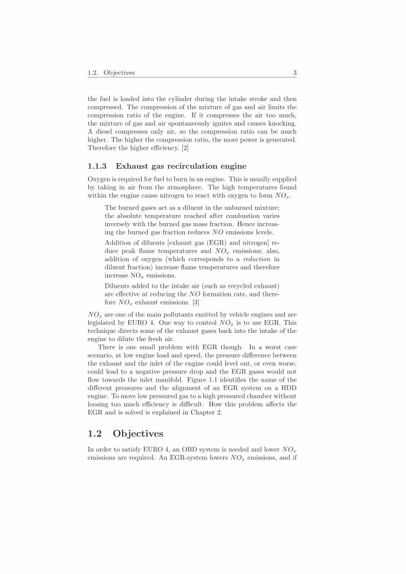
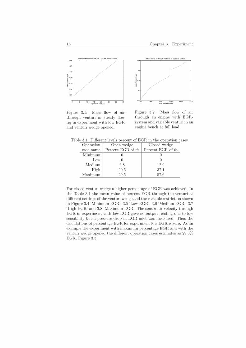
A steady flow rig is the existing laboratory equipment available.Since this rig is used, correct air mass flow through the venturi maybe difficult to achieve because the use of an air pump instead of anair compressor1. Figure 3.1 an Figure 3.2 illustrates the differencesbetween the steady flow rigs maximum mass flow and the mass flow inan engine with compressor. Air will flow the correct way and the samedirection but with less pressure and less mass of air. About one thirdof the air mass flow in the engine bench is achieved with the steadyflow rig. [6] If correct air velocity is achieved, higher mass flow in theengine bench leads to higher density. However it is assumed that notusing correct air mass flow does not affect the result of modelling theEGR to much.
More important is to achieve velocity corresponding to air velocitiesin the real EGR since it is likely that air velocity is high and closeto sound velocity. As a rule of thumb air velocity more then Mach0.3 is considered compressible and close to sound velocity. [5] Due tocharacteristic of gases the velocity is more critic then air mass flow andaffect the EGR model more.
3.1 Percent exhaust gas recirculation
Ten different experiments created with five different settings on thevariable restriction at EGR inlet and two settings on the venturi wedge.
1In a HDD engine a compressor is used to feed the inlet of the engine with air.
15
16 Chapter 3. Experiment
0 5 10 15 20 25 30 350
0.02
0.04
0.06
0.08
0.1
0.12
0.14Massflow experiment with low EGR and wedge opened.
Mas
s flo
w a
ir [k
g/s]
Operation case [−]
Figure 3.1: Mass flow of airthrough venturi in steady flowrig in experiment with low EGRand venturi wedge opened.
1000 1200 1400 1600 1800 20000.25
0.3
0.35
0.4
0.45
Engine speed [rpm]
Mas
s flo
w a
ir [k
g/s]
Mass flow of air through venturi in an engine at full load
Figure 3.2: Mass flow of airthrough an engine with EGR-system and variable venturi in anengine bench at full load.
Table 3.1: Different levels percent of EGR in the operation cases.Operation Open wedge Closed wedgecase name Percent EGR of m Percent EGR of mMinimum 0 0
Low 0 0Medium 6.8 12.9
High 20.5 37.1Maximum 29.5 57.6
For closed venturi wedge a higher percentage of EGR was achieved. Inthe Table 3.1 the mean value of percent EGR through the venturi atdifferent settings of the venturi wedge and the variable restriction shownin Figure 3.4 ‘Minimum EGR’, 3.5 ‘Low EGR’, 3.6 ‘Medium EGR’, 3.7‘High EGR’ and 3.8 ‘Maximum EGR’. The sensor air velocity throughEGR in experiment with low EGR gave no output reading due to lowsensibility but a pressure drop in EGR inlet was measured. Thus thecalculations of percentage EGR for experiment low EGR is zero. As anexample the experiment with maximum percentage EGR and with theventuri wedge opened the different operation cases estimates as 29.5%EGR, Figure 3.3.

3.1. Percent exhaust gas recirculation 17
0 5 10 15 20 25 30 35 400
5
10
15
20
25
30
Per
cent
EG
R [%
]
Operation case [−]
Percent EGR of mass flow air
Figure 3.3: Percentage EGR at different operation cases in experimentwith maximum EGR and venturi wedge opened. The result is estimatedas a mean value of 29.5% EGR.
Figure 3.4: Picture of re-striction position when do-ing EGR flow experiment,called minimum or no EGR.
Figure 3.5: Picture of re-striction position when do-ing EGR flow experiment,low EGR.

18 Chapter 3. Experiment
Figure 3.6: Picture of re-striction position when do-ing EGR flow experiment,medium EGR.
Figure 3.7: Picture of re-striction position when do-ing EGR flow experiment,high EGR.
3.1. Percent exhaust gas recirculation 19
Figure 3.8: Picture of re-striction position when do-ing EGR flow experiment,maximum EGR.
�
�
���
��
�
��
� �
��
��
��
�
���
��
��
��
�!��
�
��
�
��������
"��
�
Figure 3.9: Schematic layout ofexperiment plant, the steady flowrig setup.

20 Chapter 3. Experiment
3.2 Collecting data
The setup of the experiment is shown in Figure 3.9 and the differentchannels are labelled from one to nine. The nine different quantities ofthe experiment is recorded during ten different series of data collectionas explained in Section 3.1.
1. m, Mass flow sensor.
2. V , Volume flow.
3. P, Pressure, before volume flow sensor.
4. PEGR, Pressure, after EGR cooler, before venturi.
5. PIM , Pressure, in inlet manifold.
6. TIM , Temperature, in inlet manifold.
7. P7, Pressure, after inlet manifold.
8. PIC , Pressure after mass flow sensor.
9. vEGR, Velocity of air through EGR after EGR cooler, before ven-turi.
To be able to create a model, the EGR mass flow, the mass flow beforethe venturi m, the temperature before the venturi T0, the pressure be-fore and the pressure in the critical section in the venturi are needed.The five remaining sensors were measured for redundance and calibra-tion.
3.2.1 Pressure and temperature sensor
As explained earlier in Chapter 2, pressure and temperature in inletmanifold is required to be able to estimate EGR mass flow. On thereal engine, there is a sensor placed in the inlet manifold which ismounted on the end of the venturi’s diffusor. Therefore, the samesensor mounted at the same place is measured during experiment togive some information about how it will behave when mounted in areal engine. To calculate the pressure in the inlet manifold an equationwas given
Uout =Uref
5114
(16P − 1) (3.1)
where Uout was measured and logged and PIM = P . [7] Uref was setat 5 volts.
The calibration of the final models from Chapter 2 depends on whichpressure sensor is used. From Section 3.2 the two sensors P7 and PIM
3.2. Collecting data 21
0 5 10 15 20 25 30 359.2
9.3
9.4
9.5
9.6
9.7
9.8
9.9
10
10.1x 10
4 Minimum EGR, wedge openP
ress
ure
[Pa]
Operation case [−]
Sensor 5Sensor 7
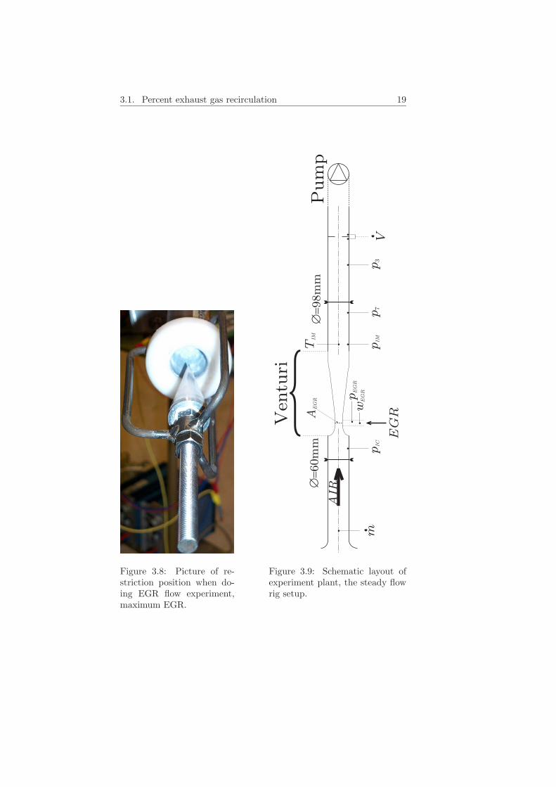
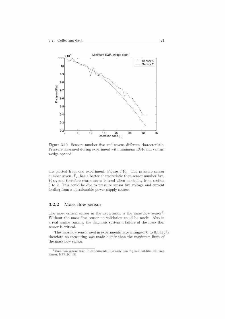
Figure 3.10: Sensors number five and sevens different characteristic.Pressure measured during experiment with minimum EGR and venturiwedge opened.
are plotted from one experiment, Figure 3.10. The pressure sensornumber seven, P7, has a better characteristic then sensor number five,PIM , and therefore sensor seven is used when modelling from section0 to 2. This could be due to pressure sensor five voltage and currentfeeding from a questionable power supply source.
3.2.2 Mass flow sensor
The most critical sensor in the experiment is the mass flow sensor2.Without the mass flow sensor no validation could be made. Also ina real engine running the diagnosis system a failure of the mass flowsensor is critical.
The mass flow sensor used in experiments have a range of 0 to 0.14 kg/stherefore no measuring was made higher than the maximum limit ofthe mass flow sensor.
2Mass flow sensor used in experiments in steady flow rig is a hot-film air-masssensor, HFM2C. [8]

22 Chapter 3. Experiment
3.3 Translate data
Different operation cases were used to be able to repeat and reproducethe data collection. The mass flow through the venturi was controlledby a pump. When a sensor saturated, the experiment was aborted.
To collect and save sensor output voltage, a PC was used. For eachoperation case, 100 samples from all eight channels was saved with asample time of 0.1 s. After an experiment was aborted a plot of all datalooks like Figure 3.11.
• Remove five highest and lowest values of the 100 measured datain a operation case, calculate the mean value of the remainingdata.
• For each operation case, remove the remaining data if a sensor issaturated.
• Calculate the absolute value in SI units.
Different sensors was saturated in different experiments due to differentsettings of the variable restriction in the inlet of EGR and the venturiwedge.
3.4 Air velocity
From Section 2.1 and the law of conservation of mass, (2.3) is m = ρwAat the given section. The velocity is calculated at section indexed 0before the venturi, the critical section index ∗ and after the venturiindex 2. The two different areas at the critical section are used tocalculate the different velocities at that section. The smaller area whenthe venturi wedge is closed and thus the greater area when calculatingopened venturi wedge.

3.4. Air velocity 23
0 1000 2000 3000 4000 5000−2
−1
0
1
2
3
4
5
6
7
Vol
tage
, [V
]
Sampel
0% EGR, wedge open
Figure 3.11: Voltage measured from experiment with minimum EGRand venturi wedge opened.

Chapter 4
Results
This chapter will present the results of the experiments from the steadyflow rig and how the models correspond to the measured data. Bothfrom section 0 to ∗ and 0 to 2. All result figures and tables from modelfitting are listed in Appendix B.
4.1 Model fitting
The Figure 4.1 shows the result of model 1 approximating the mass flowwith the pressure p0 and p∗. The data from the experiment plotted iswith medium EGR, approximately 13 percent, and the venturi wedgeclosed. The X-axis is the modelled mass flow and the Y-axis is themeasured mass flow.
The Figure 4.2 shows the residual of the result in Figure 4.1. Thefit residuals are defined as the difference between the ordinate datapoint and the resulting fit for each abscissa data point. The Table 4.1is a summation of the coefficients, norm and standard deviation forexperiment from section 0 to ∗ with closed venturi wedge.
Table 4.1: Results of fittings. Model 1, section 0 to ∗.Coefficients, Coefficients, Norm of Standard
Experiment p1 p2 residuals deviationMinimum closed 0.97117 0.00046634 0.0020747 0.385e-003
Low closed 0.98886 0.00038561 0.0026826 0.467e-003Medium closed 0.99858 0.00054486 0.0033943 0.566e-003
High closed 1.0447 0.0030482 0.007653 1.154e-003Maximum closed 2.9585 0.0021822 0.027442 4.639e-003
24

4.1. Model fitting 25
0 0.1 0.2 0.3 0.4 0.5 0.60
0.02
0.04
0.06
0.08
0.1
0.12
0.14
0.16
0.18M
ass
flow
[kg/
s]
Mass flow [kg/s]
Measured and modeled mass flow through the venturi
Figure 4.1: Result of model 1 from 0 to ∗, experiment medium EGRand closed wedge.
0 0.1 0.2 0.3 0.4 0.5 0.6−2.5
−2
−1.5
−1
−0.5
0
0.5
1
1.5
2
2.5x 10
−3
Mass flow [kg/s]
Am
plid
ude
of r
esid
uals
[kg/
s]
Residuals
Figure 4.2: Residual of model 1 from 0 to ∗, experiment medium EGRand closed wedge.

26 Chapter 4. Results
0 0.1 0.2 0.3 0.4 0.5 0.60
0.02
0.04
0.06
0.08
0.1
0.12
0.14
0.16
0.18
Mas
s flo
w [k
g/s]
Mass flow [kg/s]
Measured and modeled mass flow through the venturi
Figure 4.3: Model 1 from section0 to ∗ with maximum EGR andopened venturi wedge.
0 0.1 0.2 0.3 0.4 0.5 0.60
0.02
0.04
0.06
0.08
0.1
0.12
0.14
0.16
0.18
Mas
s flo
w [k
g/s]
Mass flow [kg/s]
Measured and modeled mass flow through the venturi
Figure 4.4: Model 1 from section0 to ∗ with maximum EGR andclosed venturi wedge.
4.1.1 Venturi model 1
Model 1 uses (2.12) to model the mass flow. The model plotted againstthe measured data is estimated as a straight line corresponding to equa-tion y = p1∗x+p2. For an example, the equation for the straight drawnline in Figure 4.1 is y ≈ x+0.5×10⁻³ and the coefficients can be foundin Table 4.1. The one constant not fixed in the models is used to ap-proximate the actual mass flow and is the discharge coefficient CD.The discharge coefficient is equal with the coefficient p1 in the tables.Steeper slope of the straight line in Figure 4.1 is a greater CD and agreater resistance to the flow of air through the venturi. ‖r‖2 of theresidual is also found in the same table and is 3.3943 × 10⁻³. In thesame table the standard deviation is calculated and is for the sameexperiment 0.566 × 10⁻³. Lower ‖r‖2 and lower standard deviation isbetter fit of the straight line.
Figure 4.3 and Figure 4.4 illustrates the worsest fit within the exper-iment. The experiment is with opened and closed venturi wedge withmaximum EGR when modelling from section 0 to ∗. Standard devia-tion of the fit from experiment with opened wedge is ‖r‖2 = 6.2×10⁻³
and for the experiment with closed wedge it is ‖r‖2 = 4.6×10⁻³. Whatcan be noticed in the figures are, the slope of the straight lines are notequal.
4.1.2 Venturi model 2
Model 2 differs from previous model with one assumption. The initialvelocity of air before entering the variable venturi is assumed to be zeroand neglected.
The two Figures 4.5 and 4.6 illustrates the worse fit with opened andclosed venturi wedge. Maximum EGR in experiment when modelling

4.1. Model fitting 27
0 0.1 0.2 0.3 0.4 0.5 0.60
0.02
0.04
0.06
0.08
0.1
0.12
0.14
0.16
0.18
Mas
s flo
w [k
g/s]
Mass flow [kg/s]
Measured and modeled mass flow through the venturi
Figure 4.5: Model 2 from section0 to ∗ with maximum EGR andopened venturi wedge.
0 0.1 0.2 0.3 0.4 0.5 0.60
0.02
0.04
0.06
0.08
0.1
0.12
0.14
0.16
0.18
Mas
s flo
w [k
g/s]
Mass flow [kg/s]
Measured and modeled mass flow through the venturi
Figure 4.6: Model 2 from section0 to ∗ with maximum EGR andclosed venturi wedge.
0 0.1 0.2 0.3 0.4 0.5 0.60
0.02
0.04
0.06
0.08
0.1
0.12
0.14
0.16
0.18
Mas
s flo
w [k
g/s]
Mass flow [kg/s]
Measured and modeled mass flow through the venturi
Figure 4.7: Model 3 from section0 to ∗ with maximum EGR andopened venturi wedge.
0 0.1 0.2 0.3 0.4 0.5 0.60
0.02
0.04
0.06
0.08
0.1
0.12
0.14
0.16
0.18
Mas
s flo
w [k
g/s]
Mass flow [kg/s]
Measured and modeled mass flow through the venturi
Figure 4.8: Model 3 from section0 to ∗ with maximum EGR andclosed venturi wedge.
from section 0 to ∗.Similar characteristic between the different experiments as in model
1 can be noticed for model 2. The slope differs if the wedge is openedor closed and differs if the percentage EGR changes.
4.1.3 Venturi model 3
Model 3 differs from model 2 and therefore also differs from model1. The difference between model 2 and model 3 is that in model 3assumes the air flow to be incompressible. Figure 4.7 and 4.8 illustratesthe worse fit with opened and closed venturi wedge. Maximum EGRin experiment when modelling from section 0 to ∗. The slope of thestraight lines in the figures are almost the same.

28 Chapter 4. Results
0 5 10 15 20 25 300
1
2
3
4
5
6
x 10−3
Sta
ndar
d de
viat
ion
of r
esid
uals
[−]
Mean value percent EGR [%]
Standard deviation at different EGR
Model 1Model 2Model 3
Figure 4.9: Standard deviation of the residuals from experiment mod-elled with the sections of 0 to 2 and the venturi wedge opened.
4.2 Residual results
The figures presented in this chapter are a collection of all results stan-dard deviation plotted against the mean value of percentage EGR. Theidea is to prove differences between the models depending on EGRpercentage.
First the Figures 4.9 and 4.10 are plotted with the modelled valuefrom section 0 to section 2 with opened or closed venturi wedge for allthree models.
As the two previous figures the next two Figure 4.11 and 4.12 arethe results to prove that the model can be used to model from sections0 to ∗ with opened or closed venturi wedge.
Figure 4.13 and 4.14 are the result with both opened and closedventuri wedge of the modelled value from sections 0 to 2 and fromsections 0 to ∗. What is important in these figures are how the modelsbehave comparing to percentage EGR and not how the different settingson the venturi wedge change the result.

4.2. Residual results 29
0 10 20 30 40 50 600
1
2
3
4
5
6
x 10−3
Sta
ndar
d de
viat
ion
of r
esid
uals
[−]
Mean value percent EGR [%]
Standard deviation at different EGR
Model 1Model 2Model 3
Figure 4.10: Standard deviation of the residuals from experiment mod-elled 0 to 2 and closed wedge.
0 5 10 15 20 25 300
1
2
3
4
5
6
x 10−3
Sta
ndar
d de
viat
ion
of r
esid
uals
[−]
Mean value percent EGR [%]
Standard deviation at different EGR
Model 1Model 2Model 3
Figure 4.11: Standard deviation of the residuals from experiment mod-elled 0 to ∗ and opened wedge.

30 Chapter 4. Results
0 10 20 30 40 50 600
1
2
3
4
5
6
x 10−3
Sta
ndar
d de
viat
ion
of r
esid
uals
[−]
Mean value percent EGR [%]
Standard deviation at different EGR
Model 1Model 2Model 3
Figure 4.12: Standard deviation of the residuals from experiment mod-elled 0 to ∗ and closed wedge.
0 10 20 30 40 50 600
1
2
3
4
5
6
x 10−3
Sta
ndar
d de
viat
ion
of r
esid
uals
[−]
Mean value percent EGR [%]
Standard deviation at different EGR
Model 1Model 2Model 3
Figure 4.13: Standard deviation of the residuals from both experimentmodelled 0 to 2, opened and closed wedge.
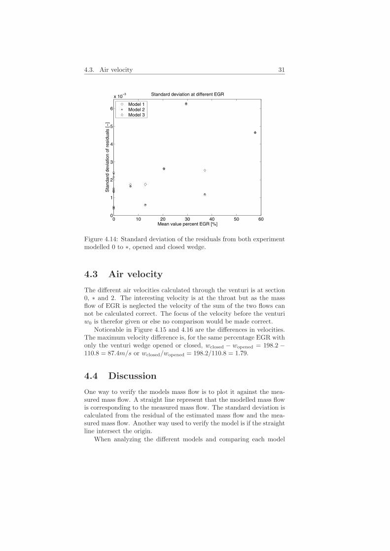
4.3. Air velocity 31
0 10 20 30 40 50 600
1
2
3
4
5
6
x 10−3
Sta
ndar
d de
viat
ion
of r
esid
uals
[−]
Mean value percent EGR [%]
Standard deviation at different EGR
Model 1Model 2Model 3
Figure 4.14: Standard deviation of the residuals from both experimentmodelled 0 to ∗, opened and closed wedge.
4.3 Air velocity
The different air velocities calculated through the venturi is at section0, ∗ and 2. The interesting velocity is at the throat but as the massflow of EGR is neglected the velocity of the sum of the two flows cannot be calculated correct. The focus of the velocity before the venturiw0 is therefor given or else no comparison would be made correct.
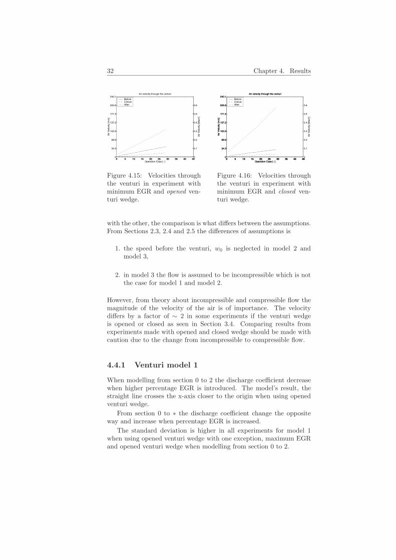
Noticeable in Figure 4.15 and 4.16 are the differences in velocities.The maximum velocity difference is, for the same percentage EGR withonly the venturi wedge opened or closed, wclosed − wopened = 198.2 −110.8 = 87.4m/s or wclosed/wopened = 198.2/110.8 = 1.79.
4.4 Discussion
One way to verify the models mass flow is to plot it against the mea-sured mass flow. A straight line represent that the modelled mass flowis corresponding to the measured mass flow. The standard deviation iscalculated from the residual of the estimated mass flow and the mea-sured mass flow. Another way used to verify the model is if the straightline intersect the origin.
When analyzing the different models and comparing each model
32 Chapter 4. Results
0 5 10 15 20 25 30 35 40 450
34.3
68.6
102.9
137.2
171.5
205.8
240.1
Air
Vel
ocity
[m/s
]
Operation Case [−]
Air velocity through the venturi
BeforeCriticalAfter
0 5 10 15 20 25 30 35 40 450
0.1
0.2
0.3
0.4
0.5
0.6
Air
Vel
ocity
[Mac
h]
Figure 4.15: Velocities throughthe venturi in experiment withminimum EGR and opened ven-turi wedge.
0 5 10 15 20 25 30 35 40 450
34.3
68.6
102.9
137.2
171.5
205.8
240.1
Air
Vel
ocity
[m/s
]
Operation Case [−]
Air velocity through the venturi
BeforeCriticalAfter
0 5 10 15 20 25 30 35 40 450
34.3
68.6
102.9
137.2
171.5
205.8
240.1
Air
Vel
ocity
[m/s
]
Operation Case [−]
Air velocity through the venturi
BeforeCriticalAfter
0 5 10 15 20 25 30 35 40 450
0.1
0.2
0.3
0.4
0.5
0.6
Air
Vel
ocity
[Mac
h]
Figure 4.16: Velocities throughthe venturi in experiment withminimum EGR and closed ven-turi wedge.
with the other, the comparison is what differs between the assumptions.From Sections 2.3, 2.4 and 2.5 the differences of assumptions is
1. the speed before the venturi, w0 is neglected in model 2 andmodel 3,
2. in model 3 the flow is assumed to be incompressible which is notthe case for model 1 and model 2.
However, from theory about incompressible and compressible flow themagnitude of the velocity of the air is of importance. The velocitydiffers by a factor of ∼ 2 in some experiments if the venturi wedgeis opened or closed as seen in Section 3.4. Comparing results fromexperiments made with opened and closed wedge should be made withcaution due to the change from incompressible to compressible flow.
4.4.1 Venturi model 1
When modelling from section 0 to 2 the discharge coefficient decreasewhen higher percentage EGR is introduced. The model’s result, thestraight line crosses the x-axis closer to the origin when using openedventuri wedge.
From section 0 to ∗ the discharge coefficient change the oppositeway and increase when percentage EGR is increased.
The standard deviation is higher in all experiments for model 1when using opened venturi wedge with one exception, maximum EGRand opened venturi wedge when modelling from section 0 to 2.

4.4. Discussion 33
4.4.2 Venturi model 2
As previous, when modelling the model 1, the discharge coefficientchange in the same way. It decreases when modelling from 0 to 2 andincreases from 0 to ∗.
The standard deviation behaves in the same manner as for themodel 1. For experiments with opened wedge it is higher and lesscorrect. Model 1 has got 11 lower standard deviation out of 20.
As for the intersection of the models result as the straight line itcrosses the x-axis closer to the origin more often when using openedwedge. Model 1 intersect closer to the origin 19 times out of 20.
4.4.3 Venturi model 3
The model 3 discharge coefficient decreases with higher percentageEGR when modelling from section 0 to 2 and increases when modellingfrom 0 to ∗.
As the other two models, when modelling with opened venturiwedge, the intersection of the x-axis and the straight line, representingmodel 3, is closer to origin and thus a better fit. Model 1 intersectcloser to the origin in all experiments.
As for the standard deviation, model 1 shows 15 better results outof 20 in the different experiments.
4.4.4 Residual results
The residual results from experiments with opened venturi wedge, Fig-ure 4.9 and Figure 4.11, illustrates that there is little differences be-tween the models for each EGR percentage. One data quantity differsthough. The highest EGR percentage in Figure 4.9.
Model 3 has got a less good fit than model 1 and 2 in experimentswith the venturi wedge closed, Figure 4.10 and Figure 4.12, with oneexception for the last data in Figure 4.12.
A relation depending on percent EGR and fit of the models whenmodelling between section 0 and ∗ could not be found. The amplitudeof standard deviation is increasing, as seen in Figure 4.14. However, theamplitude of the standard deviation is increasing and worsening withineach experiment when modelling from section 0 to ∗ as illustrated inFigure 4.11 and Figure 4.12.
Higher percentage EGR is achieved with lower pressure in the criti-cal section, the venturi throat. Lower pressure is achieved with greatervelocity of the medium, the air passing the throat. When closing theventuri wedge the area in the throat is reduced. Equation 2.3 givesthat a constant mass flow m and a reduced area A must increase the

34 Chapter 4. Results
product ρw. The density at the given section is when the tempera-ture is constant ρ = ρ(p∗) and the pressure will decrease and w∗ mustincrease. Consequently, experiments with closed venturi wedge leadsto greater velocities, Figure 4.15 and Figure 4.16. Model 3 assume in-compressible flow. At higher velocities, with closed venturi wedge, theflow is not incompressible and therefor shows less good fit than model 1and 2. Velocities of air through an engine at full load is compressibleand therefore model 3 is rejected, Figure 3.2.
4.4.5 Discharge coefficient
The discharge coefficient, CD change with different percentage EGR.It is not a function of only percent EGR or velocity of air. Due to thefact, that if it was a function of velocity, then it would not increase withpercentage EGR. The maximum velocity in the different experimentsare almost the same, therefore it can not be depending on velocitiesalone.
The coefficient also changes with different models for the same ex-periment. It is a complex coefficient and not a constant.
One suggestion might be that the flow of EGR is some sort of re-sistance against the mass flow through the venturi, when trying toapproximate the mass flow through the venturi with the pressure inthe throat. In the case when modelling from section 0 to 2 it makes iteasier for the flow, when increasing percentage EGR, and the coefficientdecreases. In the other case the coefficient increases when modellingfrom section 0 to ∗ for increasing mass flow EGR.

Chapter 5
Conclusions andextensions
An attempt has been made to present a model of a variable venturi thatcan be used to model the mass flow through the EGR and secondly,verify how the same model approximates the mass flow through thewhole variable venturi, from section 0 to 2.
5.1 Conclusions
If different models can approximate the pressure of the different sec-tions in the variable venturi, the mass flow in that section can also beapproximated.
Three models with different simplifications have been compared.The assumptions that vary between the models are that model 2 doesnot take the initial velocity into account but model 1 does. Whatdiffers between model 2 and model 3 is, that model 3 further assumesincompressible air flow.
It is shown that model 3 approximates the mass flow through theventuri worse, in the experiments, than the other two models for in-creasing velocities as the venturi wedge is closed. In an engine evenhigher velocities are reached and therefore model 3 is not recommendedfor modelling the venturi and the mass flow of EGR.
Model 1 has got the best fit of the three and the straight line rep-resenting model 1 cuts the x-axis closer to the origin then the othertwo models. However, model 1 is the most complex model of the threeand requires more calculations to approximate the mass flow of EGRand therefore takes more time to calculate. If model accuracy is moreimportant than the time it takes to calculate the mass flow, model 1
35
36 Chapter 5. Conclusions and extensions
is recommended otherwise model 2, if time to approximate is morecritical.
As model 2 approximates the air velocity before the venturi tozero, in a real engine when velocities are higher, the approximationcan worsen the result of the model 2.
5.2 Extensions
Possible future work with the model of a variable venturi.
Discharge coefficient The discharge coefficient should be examinedfurther. If an equation for the real air flow losses and resistancecan be found, the models approximation would be better.
Real engine experiments The models should be tried with a realengine in both static and dynamic experiments.
Diffusor separation The theory of air flow in a divergent channeldiscusses the problem of separation. Does the variable venturihave problems with separation and does increasing EGR flow en-hance the problem.
EGR mass flow The three models presented in this thesis assumethe mass flow of EGR to be very small and therefore neglected.Investigate how the model works with the mass flow of EGRincluded. Since the temperature of the EGR gases is higher, theenergy of EGR mass flow should be considered.

References
[1] Scania World Wide Web. About us. http://www.scania.com/au/,September 2002.
[2] Marshall Brain. How Diesel Engines Work.http://www.howstuffworks.com/diesel.htm, November 2002.
[3] John B. Heywood. Internal combustion engine fundamentals. Me-chanical engineering series. McGraw-Hill, Singapore, internationaledition edition, 1988.
[4] Ingvar Ekroth and Eric Granryd. Tillampad termodynamik. Instuti-tionen for Energiteknik, Avdelningen for Tillampad termodynamikoch kylteknik, Kungliga Tekniska Hogskolan, Stockholm, Sweden,1994. In Swedish.
[5] Frank W. Schmidt, Robert E. Henderson, and Carl H. Wolgemuth.Introduction to thermal sciences: thermodynamics, fluid dynamics,heat transfer. John Wiley & Sons, Inc, New York, USA, secondedition edition, 1993.
[6] Scania CV. Henrik Hoglund, NMEE. Experiment engine data. In-ternal document, Scania., March 2002.
[7] Scania CV. S. Ryhanen. Sensor temp/pressure tab dwg. specifi-cation for sensor with cable and connector. Internal document,Scania., March 2002. Part no. 1399310.
[8] BOSCH. Technical customer information. Calibration data sheet,March 1995. BOSCH Product part no. 0 280 217 119, Prod. typeHFM2C.
[9] Karl Storck, Matts Karlsson, and Dan Loyd. Formelsamling istromningslara, termodynamik och varmeoverforing. Technical Re-port LiTH-IKP-S-424, Mekanisk varmeteori och stromningslara, In-stitutionen for Konstruktions- och Produktionsteknik, Linkoping,Sweden, November 1996. Course material, Linkopings Universitet,Sweden.
37

38

Notation
Symbols used in the report. Symbols index is set corresponding to thereal engine sensor or engine part placement.
Variables and parameters
A Area m2
CD Discharge coefficient −cp Specific heat at constant pressure J/kg · Kcv Specific heat at constant pressure J/kg · KE Rate of energy transfer as work Wε Work Nm/kgg Gravitational acceleration m/s2
h Enthalpy J/kgκ Ratio of specific heats, quota cp/cv −m Mass flow rate kg/sp Pressure PaQ Heat transfer J/sρ Density kg/m3
T Temperature Kυ Specific volume m3/kgw Velocity m/sz Height m
39

Appendix A
Equations
Derivations of general equations used in this thesis is made in thisappendix.
A.1 General equations
The derivation made is to help understand simpler equation manip-ulation and the equations used is defined in [5], [4] and [9]. In theChapter 5.2, notation is found and is used instead of the literaturesdefinitions.
Density is defined as
υ =1ρ. (A.1)
Assume isentropic process, then
pυκ = const. (A.2)
Ideal gas law ispυ = RT. (A.3)
A.2 Derivations
Use new indexes as α = 0 and β = ∗ from Figure 2.1 and (A.2) then
pαυκα = pβυκ
β (A.4)
and solve for υα together with (A.3) is
υα =(
pβ
pα
) 1κ
υβ =(
pβ
pα
) 1κ RTβ
pβ. (A.5)
40

A.2. Derivations 41
Use definition of density, (A.1) then
ρα =(
pβ
pα
)− 1κ pβ
RTβ(A.6)
and the product of densities are
ρα
ρβ=
υβ
υα=(
pα
pβ
) 1κ
. (A.7)
A more specific derivation of Tβ
Tα=(
pβ
pα
)from Section2.3 and (2.8).
As previous use new indexes α and β then
(Tα − Tβ) = Tα
(1 − Tβ
Tα
)(A.8)
together with (A.4) and (A.3) is
pβ
(RTβ
pβ
)κ
= pα
(RTα
pα
)κ
. (A.9)
A rewriting and division gives(Tβ
Tα
)κ
=pα
pβ
(pβ
pα
)κ
(A.10)
and finallyTβ
Tα=(
pα
pβ
) 1κ(
pα
pβ
)−κκ
=(
pβ
pα
)κ−1κ
. (A.11)

Appendix B
Results
The most part of the plots from results and experiment are found inthis appendix.
B.1 Velocities through the venturi
Presented here is the velocities through the venturi. Theory of calcu-lations is founded in Chapter 3.4.
0 5 10 15 20 25 30 35 40 450
34.3
68.6
102.9
137.2
171.5
205.8
240.1
Air
Vel
ocity
[m/s
]
Operation Case [−]
Air velocity through the venturi
BeforeCriticalAfter
0 5 10 15 20 25 30 35 40 450
0.1
0.2
0.3
0.4
0.5
0.6
Air
Vel
ocity
[Mac
h]
Figure B.1: Velocities throughthe venturi in experiment withminimum EGR and opened ven-turi wedge.
0 5 10 15 20 25 30 35 40 450
34.3
68.6
102.9
137.2
171.5
205.8
240.1
Air
Vel
ocity
[m/s
]
Operation Case [−]
Air velocity through the venturi
BeforeCriticalAfter
0 5 10 15 20 25 30 35 40 450
34.3
68.6
102.9
137.2
171.5
205.8
240.1
Air
Vel
ocity
[m/s
]
Operation Case [−]
Air velocity through the venturi
BeforeCriticalAfter
0 5 10 15 20 25 30 35 40 450
0.1
0.2
0.3
0.4
0.5
0.6
Air
Vel
ocity
[Mac
h]
Figure B.2: Velocities throughthe venturi in experiment withminimum EGR and closed ven-turi wedge.
42

B.1. Velocities through the venturi 43
0 5 10 15 20 25 30 35 40 450
34.3
68.6
102.9
137.2
171.5
205.8
240.1
Air
Vel
ocity
[m/s
]
Operation Case [−]
Air velocity through the venturi
BeforeCriticalAfter
0 5 10 15 20 25 30 35 40 450
34.3
68.6
102.9
137.2
171.5
205.8
240.1
Air
Vel
ocity
[m/s
]
Operation Case [−]
Air velocity through the venturi
BeforeCriticalAfter
0 5 10 15 20 25 30 35 40 450
34.3
68.6
102.9
137.2
171.5
205.8
240.1
Air
Vel
ocity
[m/s
]
Operation Case [−]
Air velocity through the venturi
BeforeCriticalAfter
0 5 10 15 20 25 30 35 40 450
0.1
0.2
0.3
0.4
0.5
0.6
Air
Vel
ocity
[Mac
h]Figure B.3: Velocities throughthe venturi in experiment withlow EGR and opened venturiwedge.
0 5 10 15 20 25 30 35 40 450
34.3
68.6
102.9
137.2
171.5
205.8
240.1
Air
Vel
ocity
[m/s
]
Operation Case [−]
Air velocity through the venturi
BeforeCriticalAfter
0 5 10 15 20 25 30 35 40 450
34.3
68.6
102.9
137.2
171.5
205.8
240.1
Air
Vel
ocity
[m/s
]
Operation Case [−]
Air velocity through the venturi
BeforeCriticalAfter
0 5 10 15 20 25 30 35 40 450
34.3
68.6
102.9
137.2
171.5
205.8
240.1
Air
Vel
ocity
[m/s
]
Operation Case [−]
Air velocity through the venturi
BeforeCriticalAfter
0 5 10 15 20 25 30 35 40 450
34.3
68.6
102.9
137.2
171.5
205.8
240.1
Air
Vel
ocity
[m/s
]
Operation Case [−]
Air velocity through the venturi
BeforeCriticalAfter
0 5 10 15 20 25 30 35 40 450
0.1
0.2
0.3
0.4
0.5
0.6
Air
Vel
ocity
[Mac
h]
Figure B.4: Velocities throughthe venturi in experiment withlow EGR and closed venturiwedge.
0 5 10 15 20 25 30 35 40 450
34.3
68.6
102.9
137.2
171.5
205.8
240.1
Air
Vel
ocity
[m/s
]
Operation Case [−]
Air velocity through the venturi
BeforeCriticalAfter
0 5 10 15 20 25 30 35 40 450
34.3
68.6
102.9
137.2
171.5
205.8
240.1
Air
Vel
ocity
[m/s
]
Operation Case [−]
Air velocity through the venturi
BeforeCriticalAfter
0 5 10 15 20 25 30 35 40 450
34.3
68.6
102.9
137.2
171.5
205.8
240.1
Air
Vel
ocity
[m/s
]
Operation Case [−]
Air velocity through the venturi
BeforeCriticalAfter
0 5 10 15 20 25 30 35 40 450
34.3
68.6
102.9
137.2
171.5
205.8
240.1
Air
Vel
ocity
[m/s
]
Operation Case [−]
Air velocity through the venturi
BeforeCriticalAfter
0 5 10 15 20 25 30 35 40 450
34.3
68.6
102.9
137.2
171.5
205.8
240.1
Air
Vel
ocity
[m/s
]
Operation Case [−]
Air velocity through the venturi
BeforeCriticalAfter
0 5 10 15 20 25 30 35 40 450
0.1
0.2
0.3
0.4
0.5
0.6
Air
Vel
ocity
[Mac
h]
Figure B.5: Velocities throughthe venturi in experiment withmedium EGR and opened ven-turi wedge.
0 5 10 15 20 25 30 35 40 450
34.3
68.6
102.9
137.2
171.5
205.8
240.1
Air
Vel
ocity
[m/s
]
Operation Case [−]
Air velocity through the venturi
BeforeCriticalAfter
0 5 10 15 20 25 30 35 40 450
34.3
68.6
102.9
137.2
171.5
205.8
240.1
Air
Vel
ocity
[m/s
]
Operation Case [−]
Air velocity through the venturi
BeforeCriticalAfter
0 5 10 15 20 25 30 35 40 450
34.3
68.6
102.9
137.2
171.5
205.8
240.1
Air
Vel
ocity
[m/s
]
Operation Case [−]
Air velocity through the venturi
BeforeCriticalAfter
0 5 10 15 20 25 30 35 40 450
34.3
68.6
102.9
137.2
171.5
205.8
240.1
Air
Vel
ocity
[m/s
]
Operation Case [−]
Air velocity through the venturi
BeforeCriticalAfter
0 5 10 15 20 25 30 35 40 450
34.3
68.6
102.9
137.2
171.5
205.8
240.1
Air
Vel
ocity
[m/s
]
Operation Case [−]
Air velocity through the venturi
BeforeCriticalAfter
0 5 10 15 20 25 30 35 40 450
34.3
68.6
102.9
137.2
171.5
205.8
240.1
Air
Vel
ocity
[m/s
]
Operation Case [−]
Air velocity through the venturi
BeforeCriticalAfter
0 5 10 15 20 25 30 35 40 450
0.1
0.2
0.3
0.4
0.5
0.6
Air
Vel
ocity
[Mac
h]
Figure B.6: Velocities throughthe venturi in experiment withmedium EGR and closed venturiwedge.
0 5 10 15 20 25 30 35 40 450
34.3
68.6
102.9
137.2
171.5
205.8
240.1
Air
Vel
ocity
[m/s
]
Operation Case [−]
Air velocity through the venturi
BeforeCriticalAfter
0 5 10 15 20 25 30 35 40 450
34.3
68.6
102.9
137.2
171.5
205.8
240.1
Air
Vel
ocity
[m/s
]
Operation Case [−]
Air velocity through the venturi
BeforeCriticalAfter
0 5 10 15 20 25 30 35 40 450
34.3
68.6
102.9
137.2
171.5
205.8
240.1
Air
Vel
ocity
[m/s
]
Operation Case [−]
Air velocity through the venturi
BeforeCriticalAfter
0 5 10 15 20 25 30 35 40 450
34.3
68.6
102.9
137.2
171.5
205.8
240.1
Air
Vel
ocity
[m/s
]
Operation Case [−]
Air velocity through the venturi
BeforeCriticalAfter
0 5 10 15 20 25 30 35 40 450
34.3
68.6
102.9
137.2
171.5
205.8
240.1
Air
Vel
ocity
[m/s
]
Operation Case [−]
Air velocity through the venturi
BeforeCriticalAfter
0 5 10 15 20 25 30 35 40 450
34.3
68.6
102.9
137.2
171.5
205.8
240.1
Air
Vel
ocity
[m/s
]
Operation Case [−]
Air velocity through the venturi
BeforeCriticalAfter
0 5 10 15 20 25 30 35 40 450
34.3
68.6
102.9
137.2
171.5
205.8
240.1
Air
Vel
ocity
[m/s
]
Operation Case [−]
Air velocity through the venturi
BeforeCriticalAfter
0 5 10 15 20 25 30 35 40 450
34.3
68.6
102.9
137.2
171.5
205.8
240.1
Air
Vel
ocity
[m/s
]
Operation Case [−]
Air velocity through the venturi
BeforeCriticalAfter
0 5 10 15 20 25 30 35 40 450
0.1
0.2
0.3
0.4
0.5
0.6
Air
Vel
ocity
[Mac
h]
Figure B.7: Velocities throughthe venturi in experiment withhigh EGR and opened venturiwedge.
0 5 10 15 20 25 30 35 40 450
34.3
68.6
102.9
137.2
171.5
205.8
240.1
Air
Vel
ocity
[m/s
]
Operation Case [−]
Air velocity through the venturi
BeforeCriticalAfter
0 5 10 15 20 25 30 35 40 450
34.3
68.6
102.9
137.2
171.5
205.8
240.1
Air
Vel
ocity
[m/s
]
Operation Case [−]
Air velocity through the venturi
BeforeCriticalAfter
0 5 10 15 20 25 30 35 40 450
34.3
68.6
102.9
137.2
171.5
205.8
240.1
Air
Vel
ocity
[m/s
]
Operation Case [−]
Air velocity through the venturi
BeforeCriticalAfter
0 5 10 15 20 25 30 35 40 450
34.3
68.6
102.9
137.2
171.5
205.8
240.1
Air
Vel
ocity
[m/s
]
Operation Case [−]
Air velocity through the venturi
BeforeCriticalAfter
0 5 10 15 20 25 30 35 40 450
34.3
68.6
102.9
137.2
171.5
205.8
240.1
Air
Vel
ocity
[m/s
]
Operation Case [−]
Air velocity through the venturi
BeforeCriticalAfter
0 5 10 15 20 25 30 35 40 450
34.3
68.6
102.9
137.2
171.5
205.8
240.1
Air
Vel
ocity
[m/s
]
Operation Case [−]
Air velocity through the venturi
BeforeCriticalAfter
0 5 10 15 20 25 30 35 40 450
34.3
68.6
102.9
137.2
171.5
205.8
240.1
Air
Vel
ocity
[m/s
]
Operation Case [−]
Air velocity through the venturi
BeforeCriticalAfter
0 5 10 15 20 25 30 35 40 450
34.3
68.6
102.9
137.2
171.5
205.8
240.1
Air
Vel
ocity
[m/s
]
Operation Case [−]
Air velocity through the venturi
BeforeCriticalAfter
0 5 10 15 20 25 30 35 40 450
34.3
68.6
102.9
137.2
171.5
205.8
240.1
Air
Vel
ocity
[m/s
]
Operation Case [−]
Air velocity through the venturi
BeforeCriticalAfter
0 5 10 15 20 25 30 35 40 450
0.1
0.2
0.3
0.4
0.5
0.6
Air
Vel
ocity
[Mac
h]
Figure B.8: Velocities throughthe venturi in experiment withhigh EGR and closed venturiwedge.

44 Appendix B. Results
0 5 10 15 20 25 30 35 40 450
34.3
68.6
102.9
137.2
171.5
205.8
240.1
Air
Vel
ocity
[m/s
]
Operation Case [−]
Air velocity through the venturi
BeforeCriticalAfter
0 5 10 15 20 25 30 35 40 450
34.3
68.6
102.9
137.2
171.5
205.8
240.1
Air
Vel
ocity
[m/s
]
Operation Case [−]
Air velocity through the venturi
BeforeCriticalAfter
0 5 10 15 20 25 30 35 40 450
34.3
68.6
102.9
137.2
171.5
205.8
240.1
Air
Vel
ocity
[m/s
]
Operation Case [−]
Air velocity through the venturi
BeforeCriticalAfter
0 5 10 15 20 25 30 35 40 450
34.3
68.6
102.9
137.2
171.5
205.8
240.1
Air
Vel
ocity
[m/s
]
Operation Case [−]
Air velocity through the venturi
BeforeCriticalAfter
0 5 10 15 20 25 30 35 40 450
34.3
68.6
102.9
137.2
171.5
205.8
240.1
Air
Vel
ocity
[m/s
]
Operation Case [−]
Air velocity through the venturi
BeforeCriticalAfter
0 5 10 15 20 25 30 35 40 450
34.3
68.6
102.9
137.2
171.5
205.8
240.1
Air
Vel
ocity
[m/s
]
Operation Case [−]
Air velocity through the venturi
BeforeCriticalAfter
0 5 10 15 20 25 30 35 40 450
34.3
68.6
102.9
137.2
171.5
205.8
240.1
Air
Vel
ocity
[m/s
]
Operation Case [−]
Air velocity through the venturi
BeforeCriticalAfter
0 5 10 15 20 25 30 35 40 450
34.3
68.6
102.9
137.2
171.5
205.8
240.1
Air
Vel
ocity
[m/s
]
Operation Case [−]
Air velocity through the venturi
BeforeCriticalAfter
0 5 10 15 20 25 30 35 40 450
34.3
68.6
102.9
137.2
171.5
205.8
240.1
Air
Vel
ocity
[m/s
]
Operation Case [−]
Air velocity through the venturi
BeforeCriticalAfter
0 5 10 15 20 25 30 35 40 450
34.3
68.6
102.9
137.2
171.5
205.8
240.1
Air
Vel
ocity
[m/s
]
Operation Case [−]
Air velocity through the venturi
BeforeCriticalAfter
0 5 10 15 20 25 30 35 40 450
0.1
0.2
0.3
0.4
0.5
0.6
Air
Vel
ocity
[Mac
h]
Figure B.9: Velocities throughthe venturi in experiment withmaximum EGR and opened ven-turi wedge.
0 5 10 15 20 25 30 35 40 450
34.3
68.6
102.9
137.2
171.5
205.8
240.1
Air
Vel
ocity
[m/s
]
Operation Case [−]
Air velocity through the venturi
BeforeCriticalAfter
0 5 10 15 20 25 30 35 40 450
34.3
68.6
102.9
137.2
171.5
205.8
240.1
Air
Vel
ocity
[m/s
]
Operation Case [−]
Air velocity through the venturi
BeforeCriticalAfter
0 5 10 15 20 25 30 35 40 450
34.3
68.6
102.9
137.2
171.5
205.8
240.1
Air
Vel
ocity
[m/s
]
Operation Case [−]
Air velocity through the venturi
BeforeCriticalAfter
0 5 10 15 20 25 30 35 40 450
34.3
68.6
102.9
137.2
171.5
205.8
240.1
Air
Vel
ocity
[m/s
]
Operation Case [−]
Air velocity through the venturi
BeforeCriticalAfter
0 5 10 15 20 25 30 35 40 450
34.3
68.6
102.9
137.2
171.5
205.8
240.1
Air
Vel
ocity
[m/s
]
Operation Case [−]
Air velocity through the venturi
BeforeCriticalAfter
0 5 10 15 20 25 30 35 40 450
34.3
68.6
102.9
137.2
171.5
205.8
240.1
Air
Vel
ocity
[m/s
]
Operation Case [−]
Air velocity through the venturi
BeforeCriticalAfter
0 5 10 15 20 25 30 35 40 450
34.3
68.6
102.9
137.2
171.5
205.8
240.1
Air
Vel
ocity
[m/s
]
Operation Case [−]
Air velocity through the venturi
BeforeCriticalAfter
0 5 10 15 20 25 30 35 40 450
34.3
68.6
102.9
137.2
171.5
205.8
240.1
Air
Vel
ocity
[m/s
]
Operation Case [−]
Air velocity through the venturi
BeforeCriticalAfter
0 5 10 15 20 25 30 35 40 450
34.3
68.6
102.9
137.2
171.5
205.8
240.1
Air
Vel
ocity
[m/s
]
Operation Case [−]
Air velocity through the venturi
BeforeCriticalAfter
0 5 10 15 20 25 30 35 40 450
34.3
68.6
102.9
137.2
171.5
205.8
240.1
Air
Vel
ocity
[m/s
]
Operation Case [−]
Air velocity through the venturi
BeforeCriticalAfter
0 5 10 15 20 25 30 35 40 450
34.3
68.6
102.9
137.2
171.5
205.8
240.1
Air
Vel
ocity
[m/s
]
Operation Case [−]
Air velocity through the venturi
BeforeCriticalAfter
0 5 10 15 20 25 30 35 40 450
0.1
0.2
0.3
0.4
0.5
0.6
Air
Vel
ocity
[Mac
h]
Figure B.10: Velocities throughthe venturi in experiment withmaximum EGR and closed ven-turi wedge.
Table B.1: Maximum velocities at different sections in the venturi inexperiment with opened wedge.
Experiment Before Critical AfterMinimum 41.0 110.8 16.2
Low 42.0 113.7 16.7Medium 42.1 113.0 16.8
High 41.9 110.3 16.8Maximum 41.0 101.6 16.6
Table B.2: Maximum velocities at different sections in the venturi inexperiment with closed wedge.
Experiment Before Critical AfterMinimum 29.0 198.2 11.6
Low 29.9 205.3 12.2Medium 29.6 202.8 12.3
High 31.3 214.2 13.7Maximum 27.1 151.3 11.2

B.2. Venturi model 1 45
B.2 Venturi model 1
The result in this section, mostly from Chapter 4, are approximatedwith the model 1, found in Section 2.3. First the ten model fitting fromsection 0 to 2 in the venturi and lower in this section the ten modelfittings from section 0 to ∗. After each section, the tables is to be foundand in them the standard deviation from the different fittings.
0 0.05 0.1 0.15 0.2 0.25 0.3 0.350
0.02
0.04
0.06
0.08
0.1
0.12
0.14
0.16
0.18
Mas
s flo
w [k
g/s]
Mass flow [kg/s]
Measured and modeled mass flow through the venturi
Figure B.11: Model 1 from sec-tion 0 to 2 with minimum EGRand opened venturi wedge.
0 0.05 0.1 0.15 0.2 0.25 0.3 0.350
0.02
0.04
0.06
0.08
0.1
0.12
0.14
0.16
0.18
Mas
s flo
w [k
g/s]
Mass flow [kg/s]
Measured and modeled mass flow through the venturi
Figure B.12: Model 1 from sec-tion 0 to 2 with minimum EGRand closed venturi wedge.
0 0.05 0.1 0.15 0.2 0.25 0.3 0.350
0.02
0.04
0.06
0.08
0.1
0.12
0.14
0.16
0.18
Mas
s flo
w [k
g/s]
Mass flow [kg/s]
Measured and modeled mass flow through the venturi
Figure B.13: Model 1 from sec-tion 0 to 2 with low EGR andopened venturi wedge.
0 0.05 0.1 0.15 0.2 0.25 0.3 0.350
0.02
0.04
0.06
0.08
0.1
0.12
0.14
0.16
0.18
Mas
s flo
w [k
g/s]
Mass flow [kg/s]
Measured and modeled mass flow through the venturi
Figure B.14: Model 1 from sec-tion 0 to 2 with low EGR andclosed venturi wedge.

46 Appendix B. Results
0 0.05 0.1 0.15 0.2 0.25 0.3 0.350
0.02
0.04
0.06
0.08
0.1
0.12
0.14
0.16
0.18
Mas
s flo
w [k
g/s]
Mass flow [kg/s]
Measured and modeled mass flow through the venturi
Figure B.15: Model 1 from sec-tion 0 to 2 with medium EGRand opened venturi wedge.
0 0.05 0.1 0.15 0.2 0.25 0.3 0.350
0.02
0.04
0.06
0.08
0.1
0.12
0.14
0.16
0.18
Mas
s flo
w [k
g/s]
Mass flow [kg/s]
Measured and modeled mass flow through the venturi
Figure B.16: Model 1 from sec-tion 0 to 2 with medium EGRand closed venturi wedge.
0 0.05 0.1 0.15 0.2 0.25 0.3 0.350
0.02
0.04
0.06
0.08
0.1
0.12
0.14
0.16
0.18
Mas
s flo
w [k
g/s]
Mass flow [kg/s]
Measured and modeled mass flow through the venturi
Figure B.17: Model 1 from sec-tion 0 to 2 with high EGR andopened venturi wedge.
0 0.05 0.1 0.15 0.2 0.25 0.3 0.350
0.02
0.04
0.06
0.08
0.1
0.12
0.14
0.16
0.18M
ass
flow
[kg/
s]
Mass flow [kg/s]
Measured and modeled mass flow through the venturi
Figure B.18: Model 1 from sec-tion 0 to 2 with high EGR andclosed venturi wedge.
0 0.05 0.1 0.15 0.2 0.25 0.3 0.350
0.02
0.04
0.06
0.08
0.1
0.12
0.14
0.16
0.18
Mas
s flo
w [k
g/s]
Mass flow [kg/s]
Measured and modeled mass flow through the venturi
Figure B.19: Model 1 from sec-tion 0 to 2 with maximum EGRand opened venturi wedge.
0 0.05 0.1 0.15 0.2 0.25 0.3 0.350
0.02
0.04
0.06
0.08
0.1
0.12
0.14
0.16
0.18
Mas
s flo
w [k
g/s]
Mass flow [kg/s]
Measured and modeled mass flow through the venturi
Figure B.20: Model 1 from sec-tion 0 to 2 with maximum EGRand closed venturi wedge.

B.2. Venturi model 1 47
Table B.3: Results of fittings. Model 1, section 0 to 2.Coefficients, Coefficients, Norm of Standard
Experiment p1 p2 residuals deviationMinimum opened 1.0157 0.0042773 0.0093283 1.732e-003
Low opened 1.0017 0.0024589 0.0097047 1.743e-003Medium opened 0.98349 0.00056242 0.0078713 1.391e-003
High opened 0.94146 0.00012837 0.010691 1.861e-003Maximum opened 0.86695 0.0016089 0.0069057 1.167e-003
Table B.4: Results of fittings. Model 1, section 0 to 2.Experiment Coefficients, Coefficients, Norm of Standard
p1 p2 residuals deviationMinimum closed 1.51 0.0043754 0.004211 0.782e-003
Low closed 1.3984 0.0039437 0.006802 1.184e-003Medium closed 1.2937 0.0043287 0.0080386 1.340e-003
High closed 1.1781 0.0037128 0.0078101 1.177e-003Maximum closed 1.2429 0.0038986 0.010366 1.752e-003
0 0.1 0.2 0.3 0.4 0.5 0.60
0.02
0.04
0.06
0.08
0.1
0.12
0.14
0.16
0.18
Mas
s flo
w [k
g/s]
Mass flow [kg/s]
Measured and modeled mass flow through the venturi
Figure B.21: Model 1 from sec-tion 0 to ∗ with minimum EGRand opened venturi wedge.
0 0.1 0.2 0.3 0.4 0.5 0.60
0.02
0.04
0.06
0.08
0.1
0.12
0.14
0.16
0.18
Mas
s flo
w [k
g/s]
Mass flow [kg/s]
Measured and modeled mass flow through the venturi
Figure B.22: Model 1 from sec-tion 0 to ∗ with minimum EGRand closed venturi wedge.
Table B.5: Results of fittings. Model 1, section 0 to *.Coefficients, Coefficients, Norm of Standard
Experiment p1 p2 residuals deviationMinimum opened 0.86123 0.0032745 0.012919 2.399e-003
Low opened 0.90807 0.0010207 0.0074619 1.340e-003Medium opened 0.9388 0.00026054 0.0092119 1.628e-003
High opened 1.0925 -0.00028319 0.015077 2.625e-003Maximum opened 2.1275 -0.00079254 0.036941 6.244e-003

48 Appendix B. Results
0 0.1 0.2 0.3 0.4 0.5 0.60
0.02
0.04
0.06
0.08
0.1
0.12
0.14
0.16
0.18
Mas
s flo
w [k
g/s]
Mass flow [kg/s]
Measured and modeled mass flow through the venturi
Figure B.23: Model 1 from sec-tion 0 to ∗ with low EGR andopened venturi wedge.
0 0.1 0.2 0.3 0.4 0.5 0.60
0.02
0.04
0.06
0.08
0.1
0.12
0.14
0.16
0.18
Mas
s flo
w [k
g/s]
Mass flow [kg/s]
Measured and modeled mass flow through the venturi
Figure B.24: Model 1 from sec-tion 0 to ∗ with low EGR andclosed venturi wedge.
0 0.1 0.2 0.3 0.4 0.5 0.60
0.02
0.04
0.06
0.08
0.1
0.12
0.14
0.16
0.18
Mas
s flo
w [k
g/s]
Mass flow [kg/s]
Measured and modeled mass flow through the venturi
Figure B.25: Model 1 from sec-tion 0 to ∗ with medium EGRand opened venturi wedge.
0 0.1 0.2 0.3 0.4 0.5 0.60
0.02
0.04
0.06
0.08
0.1
0.12
0.14
0.16
0.18M
ass
flow
[kg/
s]
Mass flow [kg/s]
Measured and modeled mass flow through the venturi
Figure B.26: Model 1 from sec-tion 0 to ∗ with medium EGRand closed venturi wedge.
0 0.1 0.2 0.3 0.4 0.5 0.60
0.02
0.04
0.06
0.08
0.1
0.12
0.14
0.16
0.18
Mas
s flo
w [k
g/s]
Mass flow [kg/s]
Measured and modeled mass flow through the venturi
Figure B.27: Model 1 from sec-tion 0 to ∗ with high EGR andopened venturi wedge.
0 0.1 0.2 0.3 0.4 0.5 0.60
0.02
0.04
0.06
0.08
0.1
0.12
0.14
0.16
0.18
Mas
s flo
w [k
g/s]
Mass flow [kg/s]
Measured and modeled mass flow through the venturi
Figure B.28: Model 1 from sec-tion 0 to ∗ with high EGR andclosed venturi wedge.

B.2. Venturi model 1 49
0 0.1 0.2 0.3 0.4 0.5 0.60
0.02
0.04
0.06
0.08
0.1
0.12
0.14
0.16
0.18
Mas
s flo
w [k
g/s]
Mass flow [kg/s]
Measured and modeled mass flow through the venturi
Figure B.29: Model 1 from sec-tion 0 to ∗ with maximum EGRand opened venturi wedge.
0 0.1 0.2 0.3 0.4 0.5 0.60
0.02
0.04
0.06
0.08
0.1
0.12
0.14
0.16
0.18
Mas
s flo
w [k
g/s]
Mass flow [kg/s]
Measured and modeled mass flow through the venturi
Figure B.30: Model 1 from sec-tion 0 to ∗ with maximum EGRand closed venturi wedge.
Table B.6: Results of fittings. Model 1, section 0 to *.Coefficients, Coefficients, Norm of Standard
Experiment p1 p2 residuals deviationMinimum closed 0.97117 0.00046634 0.0020747 0.385e-003
Low closed 0.98886 0.00038561 0.0026826 0.467e-003Medium closed 0.99858 0.00054486 0.0033943 0.566e-003
High closed 1.0447 0.0030482 0.007653 1.154e-003Maximum closed 2.9585 0.0021822 0.027442 4.639e-003

50 Appendix B. Results
B.3 Venturi model 2
The result in this section, mostly from Chapter 4, are approximatedwith the model 2, found in Section 2.4. First the ten model fitting fromsection 0 to 2 in the venturi and lower in this section the ten modelfittings from section 0 to ∗. After each section, the tables is to be foundand in them the standard deviation from the different fittings.
0 0.05 0.1 0.15 0.2 0.25 0.3 0.350
0.02
0.04
0.06
0.08
0.1
0.12
0.14
0.16
0.18
Mas
s flo
w [k
g/s]
Mass flow [kg/s]
Measured and modeled mass flow through the venturi
Figure B.31: Model 2 from sec-tion 0 to 2 with minimum EGRand opened venturi wedge.
0 0.05 0.1 0.15 0.2 0.25 0.3 0.350
0.02
0.04
0.06
0.08
0.1
0.12
0.14
0.16
0.18
Mas
s flo
w [k
g/s]
Mass flow [kg/s]
Measured and modeled mass flow through the venturi
Figure B.32: Model 2 from sec-tion 0 to 2 with minimum EGRand closed venturi wedge.
0 0.05 0.1 0.15 0.2 0.25 0.3 0.350
0.02
0.04
0.06
0.08
0.1
0.12
0.14
0.16
0.18
Mas
s flo
w [k
g/s]
Mass flow [kg/s]
Measured and modeled mass flow through the venturi
Figure B.33: Model 2 from sec-tion 0 to 2 with low EGR andopened venturi wedge.
0 0.05 0.1 0.15 0.2 0.25 0.3 0.350
0.02
0.04
0.06
0.08
0.1
0.12
0.14
0.16
0.18
Mas
s flo
w [k
g/s]
Mass flow [kg/s]
Measured and modeled mass flow through the venturi
Figure B.34: Model 2 from sec-tion 0 to 2 with low EGR andclosed venturi wedge.

B.3. Venturi model 2 51
0 0.05 0.1 0.15 0.2 0.25 0.3 0.350
0.02
0.04
0.06
0.08
0.1
0.12
0.14
0.16
0.18
Mas
s flo
w [k
g/s]
Mass flow [kg/s]
Measured and modeled mass flow through the venturi
Figure B.35: Model 2 from sec-tion 0 to 2 with medium EGRand opened venturi wedge.
0 0.05 0.1 0.15 0.2 0.25 0.3 0.350
0.02
0.04
0.06
0.08
0.1
0.12
0.14
0.16
0.18
Mas
s flo
w [k
g/s]
Mass flow [kg/s]
Measured and modeled mass flow through the venturi
Figure B.36: Model 2 from sec-tion 0 to 2 with medium EGRand closed venturi wedge.
0 0.05 0.1 0.15 0.2 0.25 0.3 0.350
0.02
0.04
0.06
0.08
0.1
0.12
0.14
0.16
0.18
Mas
s flo
w [k
g/s]
Mass flow [kg/s]
Measured and modeled mass flow through the venturi
Figure B.37: Model 2 from sec-tion 0 to 2 with high EGR andopened venturi wedge.
0 0.05 0.1 0.15 0.2 0.25 0.3 0.350
0.02
0.04
0.06
0.08
0.1
0.12
0.14
0.16
0.18
Mas
s flo
w [k
g/s]
Mass flow [kg/s]
Measured and modeled mass flow through the venturi
Figure B.38: Model 2 from sec-tion 0 to 2 with high EGR andclosed venturi wedge.
0 0.05 0.1 0.15 0.2 0.25 0.3 0.350
0.02
0.04
0.06
0.08
0.1
0.12
0.14
0.16
0.18
Mas
s flo
w [k
g/s]
Mass flow [kg/s]
Measured and modeled mass flow through the venturi
Figure B.39: Model 2 from sec-tion 0 to 2 with maximum EGRand opened venturi wedge.
0 0.05 0.1 0.15 0.2 0.25 0.3 0.350
0.02
0.04
0.06
0.08
0.1
0.12
0.14
0.16
0.18
Mas
s flo
w [k
g/s]
Mass flow [kg/s]
Measured and modeled mass flow through the venturi
Figure B.40: Model 2 from sec-tion 0 to 2 with maximum EGRand closed venturi wedge.

52 Appendix B. Results
Table B.7: Results of fittings. Model 2, section 0 to 2.Coefficients, Coefficients, Norm of Standard
Experiment p1 p2 residuals deviationMinimum opened 1.1002 0.0045204 0.0091285 1.695e-003
Low opened 1.0839 0.0027552 0.0094432 1.696e-003Medium opened 1.0633 0.00090573 0.0079153 1.399e-003
High opened 1.0173 0.0004886 0.01053 1.833e-003Maximum opened 0.93566 0.0020095 0.007152 1.209e-003
Table B.8: Results of fittings. Model 2, section 0 to 2.Coefficients, Coefficients, Norm of Standard
Experiment p1 p2 residuals deviationMinimum closed 1.533 0.00442 0.0042731 0.793e-003
Low closed 1.419 0.0040029 0.0068785 1.197e-003Medium closed 1.3123 0.0043982 0.0081649 1.361e-003
High closed 1.1939 0.0038134 0.008042 1.212e-003Maximum closed 1.2609 0.0039609 0.010483 1.772e-003
0 0.1 0.2 0.3 0.4 0.5 0.60
0.02
0.04
0.06
0.08
0.1
0.12
0.14
0.16
0.18
Mas
s flo
w [k
g/s]
Mass flow [kg/s]
Measured and modeled mass flow through the venturi
Figure B.41: Model 2 from sec-tion 0 to ∗ with minimum EGRand opened venturi wedge.
0 0.1 0.2 0.3 0.4 0.5 0.60
0.02
0.04
0.06
0.08
0.1
0.12
0.14
0.16
0.18
Mas
s flo
w [k
g/s]
Mass flow [kg/s]
Measured and modeled mass flow through the venturi
Figure B.42: Model 2 from sec-tion 0 to ∗ with minimum EGRand closed venturi wedge.
Table B.9: Results of fittings. Model 2, section 0 to *.Experiment Coefficients, Coefficients, Norm of Standard
p1 p2 residuals deviationMinimum opened 0.93018 0.0036246 0.012568 2.334e-003
Low opened 0.98031 0.0014211 0.0072757 1.307e-003Medium opened 1.0141 0.00064106 0.0091906 1.625e-003
High opened 1.1833 -1.1933e-005 0.015025 2.616e-003Maximum opened 2.3237 -0.00084934 0.036982 6.251e-003

B.3. Venturi model 2 53
0 0.1 0.2 0.3 0.4 0.5 0.60
0.02
0.04
0.06
0.08
0.1
0.12
0.14
0.16
0.18
Mas
s flo
w [k
g/s]
Mass flow [kg/s]
Measured and modeled mass flow through the venturi
Figure B.43: Model 2 from sec-tion 0 to ∗ with low EGR andopened venturi wedge.
0 0.1 0.2 0.3 0.4 0.5 0.60
0.02
0.04
0.06
0.08
0.1
0.12
0.14
0.16
0.18
Mas
s flo
w [k
g/s]
Mass flow [kg/s]
Measured and modeled mass flow through the venturi
Figure B.44: Model 2 from sec-tion 0 to ∗ with low EGR andclosed venturi wedge.
0 0.1 0.2 0.3 0.4 0.5 0.60
0.02
0.04
0.06
0.08
0.1
0.12
0.14
0.16
0.18
Mas
s flo
w [k
g/s]
Mass flow [kg/s]
Measured and modeled mass flow through the venturi
Figure B.45: Model 2 from sec-tion 0 to ∗ with medium EGRand opened venturi wedge.
0 0.1 0.2 0.3 0.4 0.5 0.60
0.02
0.04
0.06
0.08
0.1
0.12
0.14
0.16
0.18
Mas
s flo
w [k
g/s]
Mass flow [kg/s]
Measured and modeled mass flow through the venturi
Figure B.46: Model 2 from sec-tion 0 to ∗ with medium EGRand closed venturi wedge.
0 0.1 0.2 0.3 0.4 0.5 0.60
0.02
0.04
0.06
0.08
0.1
0.12
0.14
0.16
0.18
Mas
s flo
w [k
g/s]
Mass flow [kg/s]
Measured and modeled mass flow through the venturi
Figure B.47: Model 2 from sec-tion 0 to ∗ with high EGR andopened venturi wedge.
0 0.1 0.2 0.3 0.4 0.5 0.60
0.02
0.04
0.06
0.08
0.1
0.12
0.14
0.16
0.18
Mas
s flo
w [k
g/s]
Mass flow [kg/s]
Measured and modeled mass flow through the venturi
Figure B.48: Model 2 from sec-tion 0 to ∗ with high EGR andclosed venturi wedge.

54 Appendix B. Results
0 0.1 0.2 0.3 0.4 0.5 0.60
0.02
0.04
0.06
0.08
0.1
0.12
0.14
0.16
0.18
Mas
s flo
w [k
g/s]
Mass flow [kg/s]
Measured and modeled mass flow through the venturi
Figure B.49: Model 2 from sec-tion 0 to ∗ with maximum EGRand opened venturi wedge.
0 0.1 0.2 0.3 0.4 0.5 0.60
0.02
0.04
0.06
0.08
0.1
0.12
0.14
0.16
0.18
Mas
s flo
w [k
g/s]
Mass flow [kg/s]
Measured and modeled mass flow through the venturi
Figure B.50: Model 2 from sec-tion 0 to ∗ with maximum EGRand closed venturi wedge.
Table B.10: Results of fittings. Model 2, section 0 to *.Experiment Coefficients, Coefficients, Norm of Standard
p1 p2 residuals deviationMinimum closed 0.98272 0.00061447 0.0021616 0.401e-003
Low closed 1.0006 0.0005359 0.0026446 0.460e-003Medium closed 1.0105 0.0006923 0.0035588 0.593e-003
High closed 1.0574 0.0031875 0.0079571 1.200e-003Maximum closed 3.0073 0.0021925 0.027442 4.639e-003

B.4. Venturi model 3 55
B.4 Venturi model 3
The result in this section, mostly from Chapter 4, are approximatedwith the model 3, found in Section 2.5. First the ten model fitting fromsection 0 to 2 in the venturi and lower in this section the ten modelfittings from section 0 to ∗. After each section, the tables is to be foundand in them the standard deviation from the different fittings.
0 0.05 0.1 0.15 0.2 0.25 0.3 0.350
0.02
0.04
0.06
0.08
0.1
0.12
0.14
0.16
0.18
Mas
s flo
w [k
g/s]
Mass flow [kg/s]
Measured and modeled mass flow through the venturi
Figure B.51: Model 3 from sec-tion 0 to 2 with minimum EGRand opened venturi wedge.
0 0.05 0.1 0.15 0.2 0.25 0.3 0.350
0.02
0.04
0.06
0.08
0.1
0.12
0.14
0.16
0.18
Mas
s flo
w [k
g/s]
Mass flow [kg/s]
Measured and modeled mass flow through the venturi
Figure B.52: Model 3 from sec-tion 0 to 2 with minimum EGRand closed venturi wedge.
0 0.05 0.1 0.15 0.2 0.25 0.3 0.350
0.02
0.04
0.06
0.08
0.1
0.12
0.14
0.16
0.18
Mas
s flo
w [k
g/s]
Mass flow [kg/s]
Measured and modeled mass flow through the venturi
Figure B.53: Model 3 from sec-tion 0 to 2 with low EGR andopened venturi wedge.
0 0.05 0.1 0.15 0.2 0.25 0.3 0.350
0.02
0.04
0.06
0.08
0.1
0.12
0.14
0.16
0.18
Mas
s flo
w [k
g/s]
Mass flow [kg/s]
Measured and modeled mass flow through the venturi
Figure B.54: Model 3 from sec-tion 0 to 2 with low EGR andclosed venturi wedge.

56 Appendix B. Results
0 0.05 0.1 0.15 0.2 0.25 0.3 0.350
0.02
0.04
0.06
0.08
0.1
0.12
0.14
0.16
0.18
Mas
s flo
w [k
g/s]
Mass flow [kg/s]
Measured and modeled mass flow through the venturi
Figure B.55: Model 3 from sec-tion 0 to 2 with medium EGRand opened venturi wedge.
0 0.05 0.1 0.15 0.2 0.25 0.3 0.350
0.02
0.04
0.06
0.08
0.1
0.12
0.14
0.16
0.18
Mas
s flo
w [k
g/s]
Mass flow [kg/s]
Measured and modeled mass flow through the venturi
Figure B.56: Model 3 from sec-tion 0 to 2 with medium EGRand closed venturi wedge.
0 0.05 0.1 0.15 0.2 0.25 0.3 0.350
0.02
0.04
0.06
0.08
0.1
0.12
0.14
0.16
0.18
Mas
s flo
w [k
g/s]
Mass flow [kg/s]
Measured and modeled mass flow through the venturi
Figure B.57: Model 3 from sec-tion 0 to 2 with high EGR andopened venturi wedge.
0 0.05 0.1 0.15 0.2 0.25 0.3 0.350
0.02
0.04
0.06
0.08
0.1
0.12
0.14
0.16
0.18M
ass
flow
[kg/
s]
Mass flow [kg/s]
Measured and modeled mass flow through the venturi
Figure B.58: Model 3 from sec-tion 0 to 2 with high EGR andclosed venturi wedge.
0 0.05 0.1 0.15 0.2 0.25 0.3 0.350
0.02
0.04
0.06
0.08
0.1
0.12
0.14
0.16
0.18
Mas
s flo
w [k
g/s]
Mass flow [kg/s]
Measured and modeled mass flow through the venturi
Figure B.59: Model 3 from sec-tion 0 to 2 with maximum EGRand opened venturi wedge.
0 0.05 0.1 0.15 0.2 0.25 0.3 0.350
0.02
0.04
0.06
0.08
0.1
0.12
0.14
0.16
0.18
Mas
s flo
w [k
g/s]
Mass flow [kg/s]
Measured and modeled mass flow through the venturi
Figure B.60: Model 3 from sec-tion 0 to 2 with maximum EGRand closed venturi wedge.
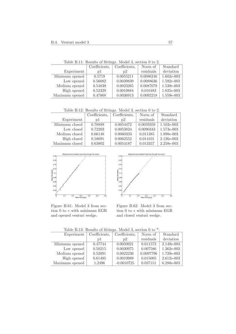
B.4. Venturi model 3 57
Table B.11: Results of fittings. Model 3, section 0 to 2.Coefficients, Coefficients, Norm of Standard
Experiment p1 p2 residuals deviationMinimum opened 0.5719 0.0055211 0.0086246 1.602e-003
Low opened 0.56082 0.0039839 0.0088636 1.592e-003Medium opened 0.54839 0.0023265 0.0087078 1.539e-003
High opened 0.52329 0.0019884 0.010483 1.825e-003Maximum opened 0.47868 0.0036913 0.0092218 1.559e-003
Table B.12: Results of fittings. Model 3, section 0 to 2.Coefficients, Coefficients, Norm of Standard
Experiment p1 p2 residuals deviationMinimum closed 0.78889 0.0054472 0.0059359 1.102e-003
Low closed 0.72203 0.0053824 0.0090343 1.573e-003Medium closed 0.66148 0.0060333 0.011385 1.898e-003
High closed 0.58691 0.0062552 0.014101 2.126e-003Maximum closed 0.63802 0.0054187 0.013357 2.258e-003
0 0.1 0.2 0.3 0.4 0.5 0.60
0.02
0.04
0.06
0.08
0.1
0.12
0.14
0.16
0.18
Mas
s flo
w [k
g/s]
Mass flow [kg/s]
Measured and modeled mass flow through the venturi
Figure B.61: Model 3 from sec-tion 0 to ∗ with minimum EGRand opened venturi wedge.
0 0.1 0.2 0.3 0.4 0.5 0.60
0.02
0.04
0.06
0.08
0.1
0.12
0.14
0.16
0.18
Mas
s flo
w [k
g/s]
Mass flow [kg/s]
Measured and modeled mass flow through the venturi
Figure B.62: Model 3 from sec-tion 0 to ∗ with minimum EGRand closed venturi wedge.
Table B.13: Results of fittings. Model 3, section 0 to *.Experiment Coefficients, Coefficients, Norm of Standard
p1 p2 residuals deviationMinimum opened 0.47744 0.0050921 0.011572 2.149e-003
Low opened 0.50215 0.0030975 0.007586 1.362e-003Medium opened 0.52091 0.0022236 0.0097796 1.729e-003
High opened 0.61495 0.0010989 0.015005 2.612e-003Maximum opened 1.2496 -0.0010725 0.037151 6.280e-003

58 Appendix B. Results
0 0.1 0.2 0.3 0.4 0.5 0.60
0.02
0.04
0.06
0.08
0.1
0.12
0.14
0.16
0.18
Mas
s flo
w [k
g/s]
Mass flow [kg/s]
Measured and modeled mass flow through the venturi
Figure B.63: Model 3 from sec-tion 0 to ∗ with low EGR andopened venturi wedge.
0 0.1 0.2 0.3 0.4 0.5 0.60
0.02
0.04
0.06
0.08
0.1
0.12
0.14
0.16
0.18
Mas
s flo
w [k
g/s]
Mass flow [kg/s]
Measured and modeled mass flow through the venturi
Figure B.64: Model 3 from sec-tion 0 to ∗ with low EGR andclosed venturi wedge.
0 0.1 0.2 0.3 0.4 0.5 0.60
0.02
0.04
0.06
0.08
0.1
0.12
0.14
0.16
0.18
Mas
s flo
w [k
g/s]
Mass flow [kg/s]
Measured and modeled mass flow through the venturi
Figure B.65: Model 3 from sec-tion 0 to ∗ with medium EGRand opened venturi wedge.
0 0.1 0.2 0.3 0.4 0.5 0.60
0.02
0.04
0.06
0.08
0.1
0.12
0.14
0.16
0.18M
ass
flow
[kg/
s]
Mass flow [kg/s]
Measured and modeled mass flow through the venturi
Figure B.66: Model 3 from sec-tion 0 to ∗ with medium EGRand closed venturi wedge.
0 0.1 0.2 0.3 0.4 0.5 0.60
0.02
0.04
0.06
0.08
0.1
0.12
0.14
0.16
0.18
Mas
s flo
w [k
g/s]
Mass flow [kg/s]
Measured and modeled mass flow through the venturi
Figure B.67: Model 3 from sec-tion 0 to ∗ with high EGR andopened venturi wedge.
0 0.1 0.2 0.3 0.4 0.5 0.60
0.02
0.04
0.06
0.08
0.1
0.12
0.14
0.16
0.18
Mas
s flo
w [k
g/s]
Mass flow [kg/s]
Measured and modeled mass flow through the venturi
Figure B.68: Model 3 from sec-tion 0 to ∗ with high EGR andclosed venturi wedge.

B.4. Venturi model 3 59
0 0.1 0.2 0.3 0.4 0.5 0.60
0.02
0.04
0.06
0.08
0.1
0.12
0.14
0.16
0.18
Mas
s flo
w [k
g/s]
Mass flow [kg/s]
Measured and modeled mass flow through the venturi
Figure B.69: Model 3 from sec-tion 0 to ∗ with maximum EGRand opened venturi wedge.
0 0.1 0.2 0.3 0.4 0.5 0.60
0.02
0.04
0.06
0.08
0.1
0.12
0.14
0.16
0.18
Mas
s flo
w [k
g/s]
Mass flow [kg/s]
Measured and modeled mass flow through the venturi
Figure B.70: Model 3 from sec-tion 0 to ∗ with maximum EGRand closed venturi wedge.
Table B.14: Results of fittings. Model 3, section 0 to *.Experiment Coefficients, Coefficients, Norm of Standard
p1 p2 residuals deviationMinimum closed 0.46362 0.0043302 0.00814 1.512e-003
Low closed 0.47109 0.0043279 0.0082298 1.433e-003Medium closed 0.4772 0.0043963 0.010448 1.741e-003
High closed 0.50221 0.0067124 0.016805 2.533e-003Maximum closed 1.5937 0.0024221 0.027461 4.642e-003

På svenska
Detta dokument hålls tillgängligt på Internet – eller dess framtida ersättare –under en längre tid från publiceringsdatum under förutsättning att inga extra-ordinära omständigheter uppstår.
Tillgång till dokumentet innebär tillstånd för var och en att läsa, ladda ner,skriva ut enstaka kopior för enskilt bruk och att använda det oförändrat för ick-ekommersiell forskning och för undervisning. Överföring av upphovsrätten viden senare tidpunkt kan inte upphäva detta tillstånd. All annan användning avdokumentet kräver upphovsmannens medgivande. För att garantera äktheten,säkerheten och tillgängligheten finns det lösningar av teknisk och administrativart.Upphovsmannens ideella rätt innefattar rätt att bli nämnd som upphovsman i denomfattning som god sed kräver vid användning av dokumentet på ovan beskrivnasätt samt skydd mot att dokumentet ändras eller presenteras i sådan form eller isådant sammanhang som är kränkande för upphovsmannens litterära eller konst-närliga anseende eller egenart.
För ytterligare information om Linköping University Electronic Press se för-lagets hemsidahttp://www.ep.liu.se/
In English
The publishers will keep this document online on the Internet - or its possiblereplacement - for a considerable time from the date of publication barring excep-tional circumstances.
The online availability of the document implies a permanent permission foranyone to read, to download, to print out single copies for your own use and touse it unchanged for any non-commercial research and educational purpose. Sub-sequent transfers of copyright cannot revoke this permission. All other uses ofthe document are conditional on the consent of the copyright owner. The pub-lisher has taken technical and administrative measures to assure authenticity,security and accessibility.
According to intellectual property law the author has the right to be men-tioned when his/her work is accessed as described above and to be protectedagainst infringement.
For additional information about the Linköping University Electronic Pressand its procedures for publication and for assurance of document integrity, pleaserefer to its WWW home page:http://www.ep.liu.se/
© [Carl-Adam Torbjörnsson]